Embed Size (px)
Citation preview

The Mixed Logit Model: The State of Practice Hensher & Greene
1
WORKING PAPER ITS-WP-02-01 The Mixed Logit Model: The State of Practice By David A. Hensher and William H. Greene January, 2002 (Revised 10 June 2002) ISSN 1440-3501
The Mixed Logit Model: The State of Practice Hensher & Greene
2
NUMBER: Working Paper ITS-WP-02-01 TITLE: The Mixed Logit Model: The State of Practice ABSTRACT: The mixed logit model is considered to be the most
promising state of the art discrete choice model currently available. Increasingly researchers and practitioners are estimating mixed logit models of various degrees of sophistication with mixtures of revealed preference and stated choice data. It is timely to review progress in model estimation since the learning curve is steep and the unwary are likely to fall into a chasm if not careful. These chasms are very deep indeed given the complexity of the mixed logit model. Although the theory is relatively clear, estimation and data issues are far from clear. Indeed there is a great deal of potential mis-inference consequent on trying to extract increased behavioural realism from data that are often not able to comply with the demands of mixed logit models. Possibly for the first time we now have an estimation method that requires extremely high quality data if the analyst wishes to take advantage of the extended behavioural capabilities of such models. This paper focuses on the new opportunities offered by mixed logit models and some issues to be aware of to avoid misuse of such advanced discrete choice methods by the practitioner.
KEY WORDS: Mixed Logit, Random Parameters, Valuation, Model
Specification, Empirical Distributions. AUTHORS: David A. Hensher and William H. Greene CONTACT: Institute of Transport Studies (Sydney & Monash) The Australian Key Centre in Transport Management, C37
The University of Sydney NSW 2006, Australia Telephone: +61 9351 0071 Facsimile: +61 9351 0088 E-mail: [email protected] Internet: http://www.its.usyd.edu.au DATE: January, 2002 (Revised 10 June 2002)

The Mixed Logit Model: The State of Practice Hensher & Greene
3
1. Introduction The logit family of models is recognised as the essential toolkit for studying discrete choices. Starting with the simple binary logit model we have progressed to the multinomial logit model (MNL) and the nested logit (NL) model, the latter becoming the most popular of the generalised logit models (see Koppelman and Sethi 2000 and Carrasco and Ortuzar 2002 for an overview). This progress occurred primarily between the mid 1960’s through to the late 1970’s. Although more advanced choice models such as the Generalised Extreme Value (GEV) and multinomial probit (MNP) models existed in conceptual and analytical form in the early 1970s, parameter estimation was seen as a practical barrier to their empirical usefulness. During the 1980’s we saw a primary focus on refinements in MNL and NL models as well as a greater understanding of their behavioural and empirical strengths and limitations (including the data requirements to assist in minimising violation of the underlying behavioural properties of the random component of the utility expression for each alternative)1. A number of software packages offered a relatively user-friendly capability to estimate MNL and NL models2. With increasing recognition of some of behavioural limitations of the closed-form MNL and NL models and the appeal of more advanced models that were analytically complex to estimate beyond three alternatives, together with the complex open-form representation of the choice probability expression, researchers focussed on finding ways to numerically estimate these models. The breakthrough came with the development of simulation methods (eg simulated maximum likelihood estimation) that enabled the open-form3 models such as multinomial probit and mixed logit to be estimated with relative ease. Papers by McFadden (1985), Börsch-Supan and Hajvassiliou (1990), Geweke et al (1994), McFadden and Ruud (1994), to name a few, all reviewed in Stern (1997), established methods to simulate the choice probabilities and estimating all parameters, by drawing pseudo-random realisations from the underlying error process (Börsch-Supan and Hajivassiliou 1990).
With estimation methods now more tractable and integrated into the popular software packages, in the mid-1990s we started seeing an increasing number of applications of mixed logit models and an accumulating knowledge base of experiences in estimating such models with available and new data sets. A close reading of this literature however revealed a concern about the general failure of advice to the analyst of many of the underlying (often not revealed) challenges that modellers experienced in arriving at a preferred model. The balance of this paper focuses on some of the most recent experiences of a number of active researchers estimating mixed logit models. Sufficient knowledge has been acquired in the last few years to be able to share some of the early practical lessons.
1 Regardless of what is said about advanced discrete choice models, the MNL model should always be the starting point for empirical investigation. It remains a major input into the modelling process, helping to ensure that the data are clean and that sensible results (eg parameter signs and significance) can be obtained from models that are not ‘cluttered’ with complex relationships (see Louviere et al 2000). 2 Although there were a number of software tools available prior to the late 1980s, the majority of analysts used Limdep (Econometric Software), Alogit (Hague Consulting Group), Quail (Brownstone) and Blogit (Hensher and Johnson 1981). Today Limdep/Nlogit and Alogit continue to be the main software packages for MNL and NL estimation with SSP also relatively popular although its development is limited. Hlogit (Börsch-Supan) and Hielow (Bierlaire) are used by a small number of researchers. GAUSS is increasing in popularity as a software language and application template for advanced discrete choice models. 3 This is in contrast to the closed form models such as MNL and NL whose probabilities can be evaluated after estimation without further analytical or numerical integration.
The Mixed Logit Model: The State of Practice Hensher & Greene
4
2. An Intuitive Description of Mixed Logit4 Like any random utility model of the discrete choice family of models, we assume that a sampled individual (q=1,…,Q) faces a choice amongst I alternatives in each of T choice situations5. An individual q is assumed to consider the full set of offered alternatives in choice situation t and to choose the alternative with the highest utility. The (relative) utility associated with each alternative i as evaluated by each individual q in choice situation t is represented in a discrete choice model by a utility expression of the general form in (1). Uitq = ßqXitq + eitq (1) Xitq is a vector of explanatory variables that are observed by the analyst (from any source) and include attributes of the alternatives, socio-economic characteristics of the respondent and descriptors of the decision context and choice task itself (eg task complexity in stated choice experiments as defined by number of choice situations, number of alternatives, attribute ranges, data collection method etc) in choice situation t, ßq and eitq are not observed by the analyst and are treated as stochastic influences. Within a logit context we impose the condition that eitq is independent and identically distributed (IID) extreme value type 1. IID is restrictive in that its does not allow for the possibility that the information relevant to making a choice that is unobserved may indeed be sufficiently rich in reality to induce correlation across the alternatives in each choice situation and indeed across choice situations. We would want to be able to take this into account in some way. One way to do this is to partition the stochastic component into two additive (ie uncorrelated) parts. One part is correlated over alternatives and heteroskedastic, and another part is IID over alternatives and individuals as shown in equation (2) (ignoring the t subscript for the present).
Uiq = β′xiq + [ηiq +εiq] (2) where ηiq is a random term with zero mean whose distribution over individuals and alternatives depends in general on underlying parameters and observed data relating to alternative i and individual q; and εiq is a random term with zero mean that is IID over alternatives and does not depend on underlying parameters or data. The Mixed Logit class of models assumes a general distribution for η and an IID extreme value type 1 distribution for ε6. That is, η can take on a number of distributional forms such as normal, lognormal, and triangular. Denote the density of η by f(η|Ω) where Ω are the fixed parameters of the distribution. For a given value of η, the conditional probability for choice i is logit, since the remaining error term is IID extreme value: 4 It is also referred to in various literatures as random parameter logit (RPL), mixed multinomial logit (MMNL), kernel logit, hybrid logit and error components logit. 5 A single choice situation refers to a set of alternatives (or choice set) from which an individual chooses one alternative. They could also rank the alternatives but we focus on first preference choice. An individual who faces a choice situation on more than one occasion (eg in a longitudinal panel) or a number of choice sets, one after the other as in stated choice experiments, is described as facing a number of choice situations. Louviere et al (2000) provide a useful introduction to discrete choice methods that use data derived from repeated choice situations, commonly known as stated choice methods. 6 The proof in McFadden and Train (2000) that mixed logit can approximate any choice model including any multinomial probit model is an important message. The reverse cannot be said: a multinomial probit model cannot approximate any mixed logit model, since multinomial probit relies critically on normal distributions. If a random term in utility is not normal, then mixed logit can handle it and multinomial probit cannot.

The Mixed Logit Model: The State of Practice Hensher & Greene
5
Li(η) = exp(β′xi + ηi) / ∑jexp(β′xj + ηj). (3)
Since η is not given, the (unconditional) choice probability is this logit formula integrated over all values of η weighted by the density of η is as shown in equation (4).
Pi=∫Li(η) f(η|Ω)dη (4) Models of this form are called mixed logit because the choice probability Li(η) is a mixture of logits with f as the mixing distribution. The probabilities do not exhibit the well known independence from irrelevant alternatives property (IIA), and different substitution patterns are obtained by appropriate specification of f. The mixed logit model recognises the role of such information and handles it in two ways (both leading to the same model only when the random effects model has a non-zero mean). The first way, known as random parameter specification, involves specifying each ßq associated with an attribute of an alternative as having both a mean and a standard deviation (ie it is treated as a random parameter instead of a fixed parameter7). The second way, known as the error components approach, treats the unobserved information as a separate error component in the random component. Since the standard deviation of a random parameter is essentially an additional error component, the estimation outcome is identical. The presence of a standard deviation of a ß parameter accommodates the presence of preference heterogeneity in the sampled population. This is often referred to as unobserved heterogeneity. While one might handle this heterogeneity through data segmentation (e.g., a different model for each trip length range, age, gender and income of each traveller – see Rizzi and Ortuzar 2002) and/or attribute segmentation (e.g., separate ßs for different trip length ranges), the challenge of these segmentation strategies is in picking the right segmentation criteria and range cut-offs and indeed being confident that one has accounted for the unobserved heterogeneity through the inclusion of observed effects. A random parameter representation of preference heterogeneity is more general; however such a specification carries a challenge in that these parameters have a distribution that is unknown. Selecting such a distribution has plenty of empirical challenges. As shown below the concern that one might not know the location of each individual’s preferences on the distribution can be accommodated by retrieving individual-specific preferences by deriving the individual’s conditional distribution based (within-sample) on their choices (ie prior knowledge). Using Bayes Rule we can define the conditional distribution as equation (5). Hq(ß|θ) = Lq(ß)g(ß|θ)/Pq(θ) (5) Lq(ß) is the likelihood of an individual’s choice if they had this specific ß; g(ß|θ) is the distribution in the population of ßs (or the probability of a ß being in the population), and Pq(θ) is the choice probability function defined in open-form as: Pq(θ) = ∫ Lq(ß)g(ß|θ) dß (6) An attractive feature of mixed logit is the ability to re-parameterise the mean estimates of random parameters to establish heterogeneity associated with observable influences. For example we can make the mean ß of travel time a linear function of one or more 7 A fixed parameter essentially treats the standard deviation as zero such that all the behavioural information is captured by the mean).

The Mixed Logit Model: The State of Practice Hensher & Greene
6
attributes (such as trip length and socio-economic characteristics). This is one way of ‘removing’ some of the unobserved heterogeneity from the parameter distribution by ‘segmenting’ the mean with continuous or discrete variation (depending on how one defines the observed influences). The choice probability in (4) or (6) cannot be calculated exactly because the integral does not have a closed form in general. The integral is approximated through simulation. For a given value of the parameters, a value of η is drawn from its distribution. Using this draw, the logit formula (3) for Li(η) is calculated. This process is repeated for many draws, and the mean of the resulting Li(η)’s is taken as the approximate choice probability giving equation (7).
SPi = (1/R)1
R
r=∑ Li(ηir) (7) R is the number of replications (i.e., draws of η), ηir is the rth draw, and SPi is the simulated probability that an individual chooses alternative i.8 The simulation method was initially introduced by Geweke (and improved by Keane, McFadden, Börsch-Supan and Hajivassiliou - see Geweke et al 1994, McFadden and Ruud 1994) of computing random variates from a multivariate truncated normal distribution. Although it fails to deliver unbiased multivariate truncated normal variates (as initially suggested by Ruud and detailed by Börsch-Supan and Hajivassiliou (1990)), it does produce unbiased estimates of the choice probabilities. The cumulative distribution function in their research is assumed to be multivariate normal and characterised by the covariance matrix M. The approach is quick and generated draws and simulated probabilities depend continuously on the parameters β and M. This latter dependence enables one to use conventional numerical methods such as quadratic hill climbing to solve the first order conditions for maximising the simulated likelihood function (equation 5) across a sample of q=1,…,Q individuals; hence the term maximum simulated likelihood (MSL) (Stern 1997).
After model estimation, there are many results for interpretation. An early warning – parameter estimates typically obtained from a random parameter or error components specification should not be interpreted as stand-alone parameters but must be assessed jointly with other linked parameter estimates. For example, the mean parameter estimate for travel time, its associated heterogeneity in mean parameter (eg. for trip length) and the standard deviation parameter estimate for travel time represent the marginal utility of travel time associated with a specific alternative and individual. The most general formula will be written out with due allowance for the distributional assumption on the random parameter. Four common specifications of the parameter distributions are those defined in equations 8a-8d using a travel time function in which we have re-parameterised the mean estimate of the travel time random parameter by trip length to establish heterogeneity associated with observable influences:
8 By construction, SPi is an unbiased estimate of Pi for any R; its variance decreases as R increases. It is strictly positive for any R, so that ln (SPi) is always defined in a log-likelihood function. It is smooth (i.e., twice differentiable) in parameters and variables, which helps in the numerical search for the maximum of the likelihood function. The simulated probabilities sum to one over alternatives. Train (1998) provides further commentary on this.

The Mixed Logit Model: The State of Practice Hensher & Greene
7
Lognormal : Exp(ßmean + ßtrip length x trip length+ ßstandard deviation×ε) (8a) Normal: ßmean + ßtrip length x trip length+ ßstandard deviation×ε (8b) Uniform: ßmean + ßtrip length x trip length+ ßspread×u (8c) Triangular: ßmean + ßtrip length x trip length+ ßspread×t (8d) where ε has a standard normal distribution, u has a uniform distribution and t has a triangular distribution. Thus far, the specification has assumed that the attributes of alternatives are independent. If we allow for attribute (ie alternative) correlation, then the random components in the preceding will be replaced with mixtures of the random components of the several parameters. (See sections 4.7 and 4.8 for more details on how to specify cross parameter correlation in the mixed logit model.)
3. Data Sources Used to Illustrate Specific Issues We will use four data sets to illustrate the range of specification, estimation and application issues in the various models. Given the focus on mixed logit models we briefly summarise their informational content and cross-reference to other sources for further details.
3.1 A Stated choice experiment for long distance car travel (Data Set 1)
A survey of long-distance road travel was undertaken in 2000, sampling residents of six cities/regional centres in New Zealand (ie Auckland, Hamilton, Palmerston North, Wellington, Christchurch, and Dunedin on both the North and South Islands). The main survey was executed as a laptop-based face-to-face interview in which each respondent was asked to complete the survey in the presence of an interviewer at their residence. Each sampled respondent evaluated 16 stated choice situations9, making two choices: the first involving choosing amongst three labelled SC alternatives and the current RP alternative, and the second choosing amongst the three SC alternatives10. A total of 274
9 A referee raised specific questions about the design of the stated choice experiments, including the ability of a respondent to handle 16 choice situations and the possibility of lexicographic and inconsistent responses. While these issues are controversial in many transport applications, it is our view that such problems often arise because stated choice designs are poorly constructed. There is a growing literature in other areas (notably marketing and environmental economics) that provides evidence of the reliability of responses to such compensatory designs which include processing of the presence of non-compensatory responses. These issues are beyond the scope of this paper and are being systematically researched in a three-year grant to the first author. 10 The development of the survey instrument occurred over the period March to October 2000. Many variations of the instrument were developed and evaluated through a series of skirmishes, pre-pilots and pilot tests. With a carefully designed experiment and presentation evolving from extensive piloting and a face to face interview process at a residential or workplace address, we have increasingly found that our tailored SC surveys with laptops are well received and understood. Answering the two choices (one after the other in each choice situation before moving to the next choice situation) is a very straightforward process which involves only one choice response if the chosen in the presence of the current trip alternative is one of the SC alternatives.

The Mixed Logit Model: The State of Practice Hensher & Greene
8
effective interviews11 with car drivers were undertaken producing 4,384 car driver cases for model estimation (ie 274×16 treatments). The choice experiment presents four alternatives to a respondent:
A. The current road the respondent is/has been using B. A hypothetical 2 lane road C. A hypothetical 4 lane road with no median D. A hypothetical 4 lane road with a wide grass median
There are two choice responses, one including all four alternatives and the other excluding the current road option. All alternatives are described by six attributes except alternative A, which does not have toll cost. Toll cost is set to zero for alternative A since there are currently no toll roads in New Zealand. The attributes in the stated choice experiment are:
1. Time on the open road which is free flow (in minutes) 2. Time on the open road which is slowed by other traffic (in minutes) 3. Percentage of total time on open road spent with other vehicles close behind
(ie tailgating) (%) 4. Curviness of the road (a four-level attribute - almost straight, slight,
moderate, winding)12 5. Running costs (in dollars) 6. Toll cost (in dollars)
These six attributes have four levels which, were chosen as follows • Free Flow Travel Time: -20%, -10%, +10%, +20% • Time Slowed Down: -20%, -10%, +10%, +20% • Percent of time with vehicles close behind: -50%, -25%, +25%, +50% • Curviness: almost straight, slight, moderate,
winding • Running Costs: -10%, -5%, +5%, +10% • Toll cost ($) for car and double for truck if trip duration is:
1. 1 hours or less 0, 0.5, 1.5, 3 2. between 1 hour and 2 hours 30 minutes 0, 1.5, 4.5, 9 3. more than 2 and a half hours 0, 2.5, 7.5, 15
The experimental design is a 46 profile in 32 choice situations. That is, there are two versions of 16 choice situations each. The design has been chosen to minimise the number of dominants in the choice situations. Within each version the order of the choice situations has been randomised to control for order effect. For example, the levels proposed for alternative B should always be different from those of alternatives C and D. The design attributes together with the choice responses and contextual data provide the information base for model estimation. An example of a stated choice screen is shown
11 We also interviewed truck drivers but they are excluded from the current empirical illustrations (See Hensher and Sullivan (2003) for the truck models). Three respondents were excluded in the estimation herein since they did not complete all 16 choice situations. 12 One referee raised a concern about a respondent’s ability to interpret degree of curviness. This issue is discussed in detail in Hensher and Sullivan (2003). In the current paper the focus is on the use of a range of data sets to illustrate the diversity of issues that mixed logit models have to address.

The Mixed Logit Model: The State of Practice Hensher & Greene
9
in Figure 1. Further details are given in Hensher and Sullivan (2003). Herein we focus only on models where individuals choose amongst the three SC alternatives.
Figure 1. An example of a stated choice screen for data set 1
3.2 A Stated choice experiment for urban commuting (Data Set 2)
A survey of a sample of 143 commuters was undertaken in late June and early July 1999 in urban New Zealand sampling residents of seven cities/regional centres (ie Auckland, Wellington, Christchurch, Palmerston North, Napier/Hastings, Nelson and Ashburton on both the North and South Islands). The main survey was executed as a laptop-based face to face interview in which each respondent was asked to complete the survey in the presence of an interviewer. Each sampled respondent evaluated 16 choice situations, choosing amongst two SC alternatives and the current (revealed preference) alternative. The 143 interviews represent 2,288 cases for model estimation (ie 143×16 treatments). The stated choice experimental design is based on two unlabelled alternatives (A and B) each defined by six attributes each of four levels (ie 412): free flow travel time, slowed up travel time, stop/crawling travel time, uncertainty of travel time, running cost and toll charges. Except for toll charges, the levels are proportions relative to those associated with a current trip identified prior to the application of the SC experiment: Free flow travel time: -0.25, -0.125, 0.125, 0.25 Slowed up travel time: -0.5, -0.25, 0.25, 0.5 Stop/crawling travel time: -0.5, -0.25, 0.25, 0.5 Uncertainty of travel time: -0.5, -0.25, 0.25, 0.5 Car running cost: -0.25, -0.125, 0.125, 0.25 Toll charges ($): 0, 2, 4, 6
The Mixed Logit Model: The State of Practice Hensher & Greene
10
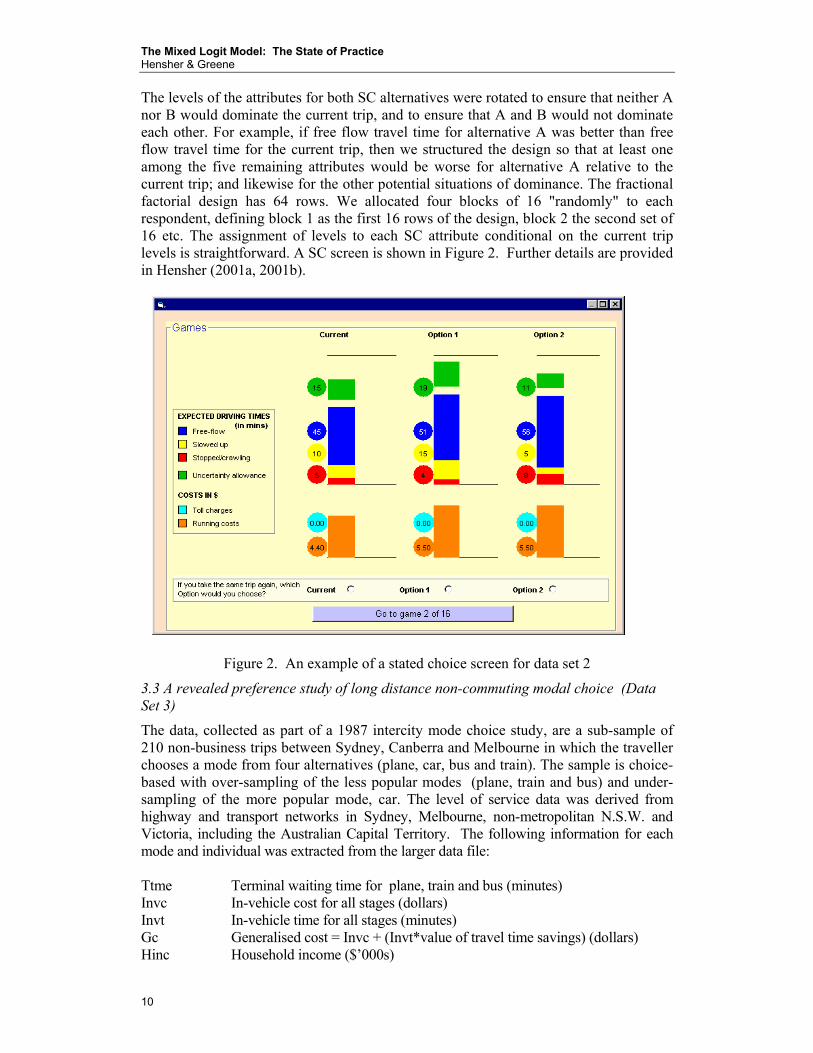
The levels of the attributes for both SC alternatives were rotated to ensure that neither A nor B would dominate the current trip, and to ensure that A and B would not dominate each other. For example, if free flow travel time for alternative A was better than free flow travel time for the current trip, then we structured the design so that at least one among the five remaining attributes would be worse for alternative A relative to the current trip; and likewise for the other potential situations of dominance. The fractional factorial design has 64 rows. We allocated four blocks of 16 "randomly" to each respondent, defining block 1 as the first 16 rows of the design, block 2 the second set of 16 etc. The assignment of levels to each SC attribute conditional on the current trip levels is straightforward. A SC screen is shown in Figure 2. Further details are provided in Hensher (2001a, 2001b).
Figure 2. An example of a stated choice screen for data set 2
3.3 A revealed preference study of long distance non-commuting modal choice (Data Set 3)
The data, collected as part of a 1987 intercity mode choice study, are a sub-sample of 210 non-business trips between Sydney, Canberra and Melbourne in which the traveller chooses a mode from four alternatives (plane, car, bus and train). The sample is choice-based with over-sampling of the less popular modes (plane, train and bus) and under-sampling of the more popular mode, car. The level of service data was derived from highway and transport networks in Sydney, Melbourne, non-metropolitan N.S.W. and Victoria, including the Australian Capital Territory. The following information for each mode and individual was extracted from the larger data file: Ttme Terminal waiting time for plane, train and bus (minutes) Invc In-vehicle cost for all stages (dollars) Invt In-vehicle time for all stages (minutes) Gc Generalised cost = Invc + (Invt*value of travel time savings) (dollars) Hinc Household income ($’000s)

The Mixed Logit Model: The State of Practice Hensher & Greene
11
Psize Travelling group size (number) Further information is given in Louviere et al (2000).
3.4 A stated choice study of urban route choice for light commercial vehicles (Data Set 4)
A stated choice experiment was designed as part of a study undertaken in 2001 in the Sydney metropolitan area to update the full set of values of travel time savings for car commuters, car non-commuters, light commercial vehicles and heavy trucks. We have selected the light commercial vehicle sub-sample of 60 interviews13 and 16 choice situations. The attributes in the design, their levels and range are summarised below:
Variables Number of levels Range
1- Free flow travel time 4 % variation from the current
2- Slowed down travel time 4 % variation from the current
3- Uncertainty in travel time 4 % variation from the current
4- Running costs 4 % variation from the current
5- Toll costs 4 $0 (free road) to $16 (double for
heavy vehicles)
6- Toll Payment: Electronic/Tag 2 Present / absent
7- Toll Payment: Cash 2 Present / absent 8- Toll Payment: Electronic/Licence plate recognition (no tag required)
2 Present / absent
Attributes 1 to 5 are based on the values for the current trip, while attributes 6 to 8 are uniquely for the SC alternatives14. In the design of the choice experiment, important considerations that needed to be accounted for were:
A. Toll should range from $0 to $16 B. A longer trip should involve higher toll alternatives. C. For a current trip without a toll, SC alternatives involving a toll should mostly be
faster than the current trip. D. We assume that the faster the road, the higher the toll; the lower the running
costs, the lower the free-flow time; and the lower the slowed down time the lower the uncertainty.
To address issue D, four nests were built. The first one is for very fast, very expensive roads. The second is for fast and expensive roads. The third is for a normal speed road and normal costs while the fourth one is for relatively inexpensive and slow roads.
13 The transport manager was interviewed together with the driver where the driver was an employee. Where the driver was the owner, he was the only person interviewed. 14 Running costs have been specified as10 litres/100Km with fuel at 97c/litre for cars and light commercial vehicles
The Mixed Logit Model: The State of Practice Hensher & Greene
12
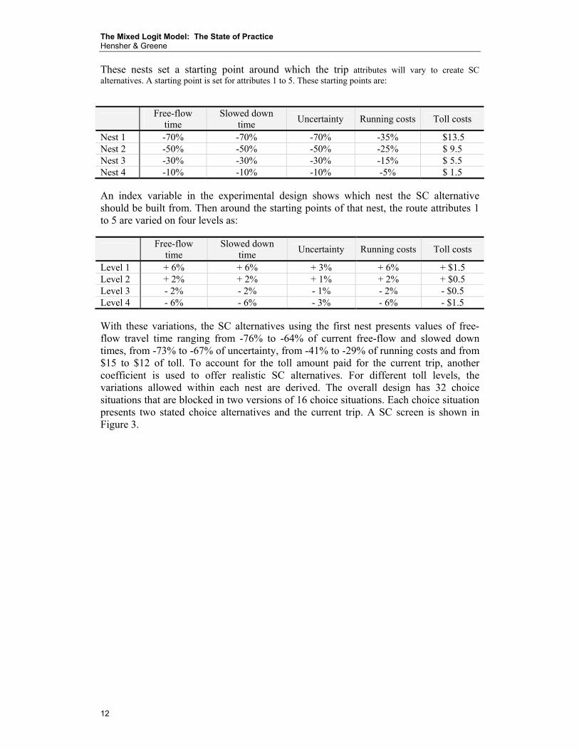
These nests set a starting point around which the trip attributes will vary to create SC alternatives. A starting point is set for attributes 1 to 5. These starting points are:
Free-flow time
Slowed down time Uncertainty Running costs Toll costs
Nest 1 -70% -70% -70% -35% $13.5 Nest 2 -50% -50% -50% -25% $ 9.5 Nest 3 -30% -30% -30% -15% $ 5.5 Nest 4 -10% -10% -10% -5% $ 1.5 An index variable in the experimental design shows which nest the SC alternative should be built from. Then around the starting points of that nest, the route attributes 1 to 5 are varied on four levels as:
Free-flow time
Slowed down time Uncertainty Running costs Toll costs
Level 1 + 6% + 6% + 3% + 6% + $1.5 Level 2 + 2% + 2% + 1% + 2% + $0.5 Level 3 - 2% - 2% - 1% - 2% - $0.5 Level 4 - 6% - 6% - 3% - 6% - $1.5 With these variations, the SC alternatives using the first nest presents values of free-flow travel time ranging from -76% to -64% of current free-flow and slowed down times, from -73% to -67% of uncertainty, from -41% to -29% of running costs and from $15 to $12 of toll. To account for the toll amount paid for the current trip, another coefficient is used to offer realistic SC alternatives. For different toll levels, the variations allowed within each nest are derived. The overall design has 32 choice situations that are blocked in two versions of 16 choice situations. Each choice situation presents two stated choice alternatives and the current trip. A SC screen is shown in Figure 3.

The Mixed Logit Model: The State of Practice Hensher & Greene
13
Figure 3. An example of a stated choice screen for data set 4
4. The Main Model Specification Issues There are at least ten key empirical issues to consider in specifying, estimating and applying a mixed logit model:
1. Selecting the parameters that are to be random parameters 2. Selecting the distribution of the random parameters 3. Specifying the way random parameters enter the model 4. Selecting the number of points on the distributions 5. Decomposing mean parameters to reflect covariate heterogeneity 6. Empirical distributions 7. Accounting for observations drawn from the same individual 8. Accounting for correlation between attributes 9. Taking advantage of priors in estimation and posteriors in application 10. Willingness to pay challenges
The differences between these key empirical issues will be explained in the following sections.
4.1 Selecting the parameters that are to be random parameters
The random parameters are the basis for accommodating correlation across alternatives (via their attributes) and across choice situations. They also define the degree of unobserved heterogeneity (via the standard deviation of the parameters) and preference heterogeneity around the mean (equivalent to an interaction between the attribute specified with a random parameter) and another attribute of an alternative, an
The Mixed Logit Model: The State of Practice Hensher & Greene
14
individual, a survey method and/or choice context. It is important to allocate a good proportion of time estimating models in which many of the attributes of alternatives are considered as having random parameters. The possibility of different distributional assumptions (see section 4.2) for each attribute should also be investigated, especially where sign is important. A warning: the findings will not necessarily be independent of the number of random draws in the simulation (see equation (7)) and so establishing the appropriate set of random parameters requires taking into account the number of draws, the distributional assumptions and, in the case of multiple choice situations per individual, whether correlated choice situations are accounted for. These interdependencies may make for a lengthy estimation process. Using the results of a base case multinomial logit model as the departure point for estimation, while helpful, cannot help in the selection of random parameterised attributes (unless extensive segmentation on each attribute within an MNL model occurs). The Lagrange Multiplier tests proposed in McFadden and Train (2000) for testing the presence of random components provides one statistical basis for accepting/rejecting the preservation of fixed parameters in the model. Brownstone (2001) provides a succinct summary of the test. These tests work by constructing artificial variables as in (9).
zin = xin − x i( )2, with x i = x jn Pjnj∑ (9)
and jnP is the conditional logit choice probability. The conditional logit model is then re-estimated including these artificial variables, and the null hypothesis of no random coefficients on attributes x is rejected if the coefficients of the artificial variables are significantly different from zero. The actual test for the joint significance of the z variables can be carried out using either a Wald or Likelihood Ratio test statistic. These Lagrange Multiplier tests can be easily carried out in any software package that estimates the conditional logit model. Brownstone suggests that these tests are easy to calculate and appear to be quite powerful omnibus tests; however, they are not as good for identifying which error components to include in a more general mixed logit specification.
4.2 Selecting the distribution of the random parameters (eg normal, lognormal, triangular, uniform)
If there is one single issue that can cause much concern it is the influence of the distributional assumptions of random parameters. The layering of selected random parameters can take a number of predefined functional forms, the most popular being normal, triangular, uniform and lognormal. The lognormal form is often used if the response parameter needs to be a specific (non-negative) sign. A uniform distribution with a (0,1) bound is sensible when we have dummy variables. Distributions are essentially arbitrary approximations to the real behavioural profile. We select specific distributions because we have a sense that the ‘empirical truth’ is somewhere in their domain. All distributions in common practice unfortunately have at least one major deficiency – typically with respect to sign and length of the tail(s). Truncated or constrained distributions appear to be the most promising direction in the future given recent concerns (see Section 4.2.4). For example, we might propose the
The Mixed Logit Model: The State of Practice Hensher & Greene
15
generalised constrained triangular in which the spread of the distribution is allowed to vary between 10% of the mean and the mean.
4.2.1 Uniform distribution
The spread of the uniform distribution (ie the distance up and down from the mean) and the standard deviation are different and the former needs to be used in representing the uniform distribution. Suppose s is the spread, such that the time coefficient is uniformly distributed from (mean-s) to (mean+s). Then the correct formula for the distribution is (mean parameter estimate + s(2u-1) where u is the uniformly distributed variable. Since the distribution of u is uniform from 0 to 1, 2u-1 is uniform from -1 to +1; then multiplying by s gives a uniform +/- s from the mean. The spread can be derived from the standard deviation by multiplying the standard deviation by 3 .
4.2.2 Triangular distribution
For the triangular distribution, the density function looks like a tent: a peak in the centre and dropping off linearly on both sides of the centre. Let c be the centre and s the spread. The density starts at c-s, rises linearly to c, and then drops linearly to c+s. It is zero below c-s and above c+s. The mean and mode are c. The standard deviation is the spread divided by 6 ; hence the spread is the standard deviation times 6 . The height of the tent at c is 1/s (such that each side of the tent has area s×(1/s)×(1/2)=1/2, and both sides have area 1/2+1/2=1, as required for a density). The slope is 1/s2. The complete density (f(x)) and cumulative distribution (F(x)) are15:
2 2 2
2 2 2
( ) 0, ( ) 0 for < - ,( ) 2[ ( )] /(2 ), ( ) [ ( )] /(2 ), ( ) ,( ) 2[( ) ] /(2 ), ( ) 1 [( ) ] /(2 ), ,( ) 0, ( ) 1, .
f x F x x c sf x x c s s F x x c s s c s x cf x c s x s F x c s x s c x c sf x F x x c s
= == − − = − − − ≤ ≤= + − = − + − < ≤ += = > +
4.2.3 Lognormal distribution
The lognormal distribution is very popular for the following reasoning. The central limit theorems explain the genesis of a normal curve. If a large number of random shocks, some positive, some negative, change the size of a particular attribute, x, in an additive fashion, the distribution of that attribute will tend to become normal as the number of shocks increases. But if these shocks act multiplicatively, changing the value of x by randomly distributed proportions instead of absolute amounts, the central limit theorems applied to Y=lnx. (where ln is to base e) tend to produce a normal distribution. Hence x has a lognormal distribution. The substitution of multiplicative for additive random shocks generates a positively skewed, leptokurtic, lognormal distribution instead of a symmetric, mesokurtic normal distribution. The degree of skewness and kurtosis of the two-parameter lognormal distribution depends only on the variance, and so if this is low enough, the lognormal approximates the normal distribution. Lognormals are appealing in that they are limited to the non-negative domain; however they typically have a very 15 Proof: Without loss of generality, let c=0. Find E[x|x>0] = s/3 and E[x|x<0] = -s/3. By integration - the conditional density is 2*unconditional density in either left or right half. In the same way, get E[x2|x>0] = s2/6 = E[x2|x<0]. This gives you the conditional variances by the expected square - squared mean. Now, the unconditional variance is the Variance of the conditional mean plus the expected value of the conditional variance. A little algebra produces the unconditional variance = s2/6. Details appear in Evans, Hasting, and Peacock (1993).

The Mixed Logit Model: The State of Practice Hensher & Greene
16
long right-hand tail which is a disadvantage (especially for willingness-to-pay calculations – see Section 4.10)16. Given the (transform) link with the normal distribution, the lognormal is best estimated with starting values from the normal. However experience suggests that they iterate many times looking for the maximum, and often get stuck along the way. The unbounded upper tail which is often behaviourally unrealistic and often quite fat does not help. Individuals typically do not have an unbounded willingness to pay for any attribute, as lognormals imply. In contrast other distributions such as the triangular and uniform are bounded on both sides, making it relatively easy to check whether the estimated bounds make sense. We will say more about the lognormal’s behavioural implications in later sections.
4.2.4 Imposing constraints on a distribution
In practice we often find that any one distribution has strengths and weaknesses. The weakness is usually associated with the spread or standard deviation of the distribution at its extremes including behaviourally unacceptable sign changes for the symmetrical distributions. The lognormal has a long upper tail. The normal, uniform and triangular give the wrong sign to some share. One appealing ‘solution’ is to make the spread or standard deviation of each random parameter a function of the mean. For example, the usual specification in terms of a normal distribution (which uses the standard deviation rather than the spread) is to define ß(i) = ß + sv(i) where v(i) is the random variable. The constrained specification would be ß (i) = ß + ßv(i) when the standard deviation equals the mean or ß(i) = ß + zßv(i) when z is a scalar taking any positive value. We would generally expect z to lie in the 0-1 range since a standard deviation (or spread) greater than the mean estimate typically17 results in behaviourally unacceptable parameter estimates.
This constraint specification can be applied to any distribution. For example, for a triangular with mean=spread, the density starts at zero, rises linearly to the mean, and then declines to zero again at twice the mean. It is peaked, like one would expect. It is bounded below at zero, bounded above at a reasonable value that is estimated, and is symmetric such that the mean is easy to interpret. It is appealing for handling willingness to pay parameters. Also with ß (i)= ß + ß v(i), where v(i) has support from -1 to +1, it does not matter if ß is negative or positive. A negative coefficient on v(i) simply reverses all the signs of the draws, but does not change the interpretation18.
4.2.5 Discrete distributions
The set of continuous distributions presented above impose a priori restrictions. An alternative is a discrete distribution. Such a distribution may be viewed as a nonparametric estimator of the random distribution. Using a discrete distribution that is identical across individuals is equivalent to a latent segmentation model with the
16 Although the ratio of two lognormals is also lognormal which is convenient result for WTP calculations despite the long tail. 17 We say typically but this is not always the case. One has to judge the findings on their own merits. 18 One could specify the relationship as ß(i)= ß+|ß|v(i), but that would create numerical problems in the optimisation routine.

The Mixed Logit Model: The State of Practice Hensher & Greene
17
probability of belonging to a segment being only a function of constants (See Ch 10 of Louviere et al (2000) for a discussion on such models). However allowing this probability to be a function of individual attributes is equivalent to allowing the points characterising the nonparametric distribution to vary across individuals. In this paper, we focus on a continuous distribution for the random components. Greene and Hensher (2002) contrast a latent class model with mixed logit.
4.2.6 An Empirical comparison of the analytical distributions
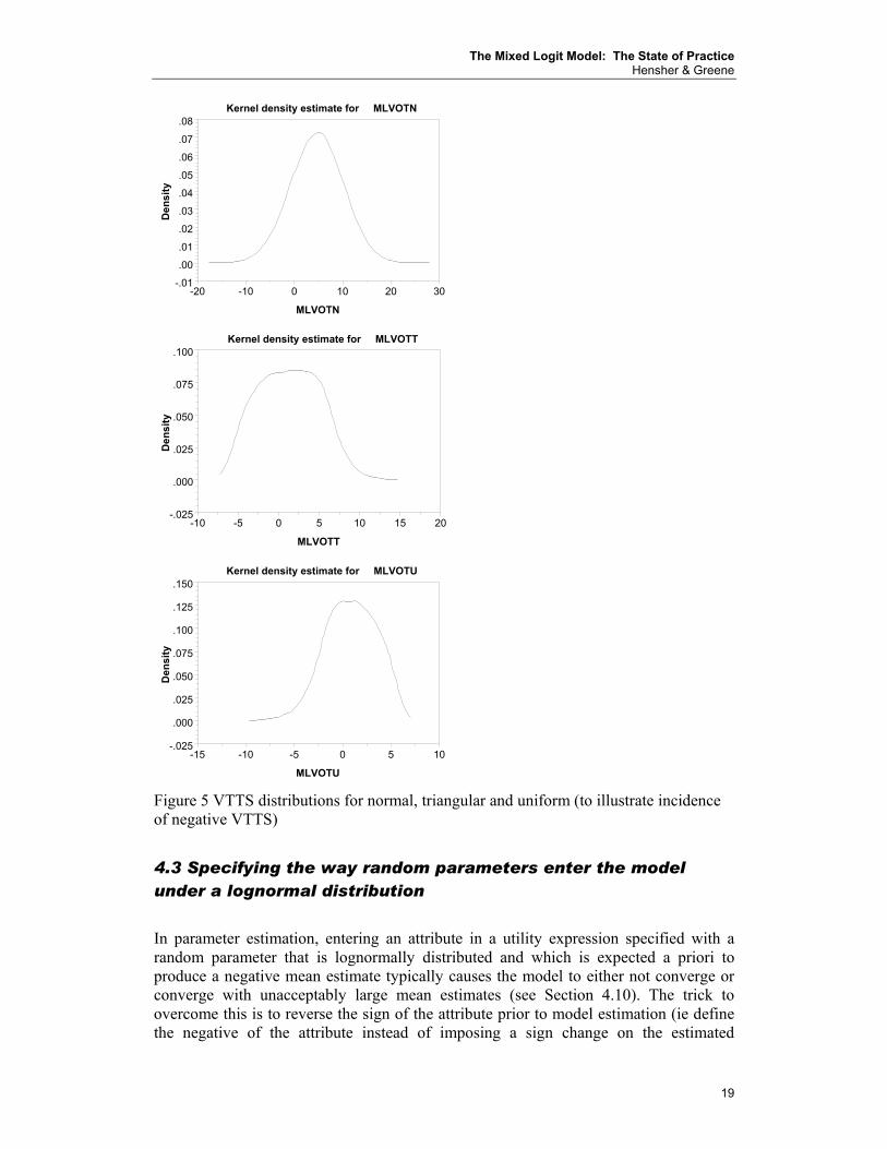
In most empirical studies, one tends to get similar means and comparable measures of spread (or standard deviation) for normal, uniform and triangular distributions19. With the lognormal, however, the evidence tends to shift around a lot, but the mean of a normal, uniform or triangular, typically existing between the mode and mean of the lognormal. This does not suggest however that we have picked the best analytical distribution to represent the true empirical distribution. This topic is investigated in some detail in Section 4.6. In Table 1 we presents some typical findings on a key behavioural output – the value of travel time savings (VTTS) using Data Set 1, noting that the standard deviation is used in the normal and lognormal distributions and the spread in the uniform and triangular distributions20. The VTTS are derived using the formulae in (8a-8d) which utilise the appropriate parameter estimates from a mixed logit model. To obtain the VTTS we divide the travel time expression by the parameter estimate for travel cost and multiply by 60 to convert from dollars per minute to dollars per hour. The VTTS distributions are plotted in Figure 4. (See Section 4.6 for discussion of how the figures are produced.) The normal, triangular and uniform are quite similar (including the overall goodness of fit of the associated models) and the lognormal is noticeably different with an unacceptably large standard deviation. The lognormal however guarantees non-negative VTTS whereas the other three (unconstrained distributions) almost certainly guarantee some negative VTTS. In this application, the percentage of VTTS that are negative for normal, triangular and uniform are respectively 19.21%, 39.33% and 37.92%.21 These percentages are obtained from a cumulative frequency distribution of VTTS.
19 One can however use different distributions on each attribute. The reason you can do this is that you are not using the distributional information in constructing the estimator. The variance estimator is based on the method of moments. Essentially, one is estimating the variance parameters just by computing sums of squares and cross products. In more detail (in response to a student inquiry) Ken Train comments that it is possible to have underlying parameters jointly normal with full covariance and then transform these underlying parameters to get the parameters that enter the utility function. For example, suppose V= α1x1+α2 x2. We can say that β1 and β2 are jointly normal with correlation and that α2 =exp(β2) and α1=β1. That gives a lognormal and a normal with correlation between them. The correlation between α2 and α2 can be calculated from the estimated correlation between β1 and β2 if you know the formula. Alternatively one can calculate it by simulating many α1 and α2 s from many draws of β1 and β2s from their estimated distribution and then calculate the correlation between the α1 and α2 s. This can be applied for any distributions. Let α2 have density g(α2) with cumulative distribution G(α2), and let α1 be normal. F(β2 |β1) is the normal CDF for β2 given β1. Then α2 is calculated as α2 =G-1(F(β2|β1)). For some Gs there must be limits on the correlation that can be attained between α1 and α2 using this procedure. 20 The estimated parameters of each model are available from the authors on request. Herein we have extracted the relevant set of parameters for the VTTS distribution expression. 21 If the analyst accidentally uses the standard deviation instead of the spread in the formula for a uniform and triangular distributions (Table 1) the mean and standard deviation for VTTS across the sample changes quite markedly (except in this case the mean for the triangular is very similar by coincidence).

The Mixed Logit Model: The State of Practice Hensher & Greene
18
Table 1. A comparison of estimates of travel time savings (Data Set 1) derived using the following formulae (tripl = trip length in minutes) (*=multiplied by):
Lognormal: mlvotl=-60*(exp(-5.40506-.0075148*tripl+2.36613*εa))/-.1048
Normal: mlvotn=60*(-.012575+.00002840*tripl+.00881228*εb)/-.10355
Triangular: mlvott=60*(-.0125428+.000028117*tripl+.0203768*T)/-.103448 where T is obtained from a standard uniform V =U[0,1] by T= 2V -1 if V<.5 or T=1-
Uniform: mlvotu=60*(-.0120956+.0000258667*tripl+.0128616*(2uc-1))/-.1032216
Value of Travel Time Savings ($ per person hour) Mean Standard Deviation Lognormal mlvotl 14.759 165.4 Normal mlvotn 4.665 5.361 Triangular mlvott 4.629 5.107a Uniform mlvotu 4.628 4.592a Using Standard Deviation instead of Spread:
Triangular mlvotts 4.636 2.588b Uniform mlvotus 2.451 2.001b Note: the standard deviation of the triangular distribution is .0203768/ 6 ; the standard deviation of a uniform distribution is.0128616/ 3 . In the last column, ‘a’ indicates that we have calculated the standard deviation for the descriptive statistics based on the application of the spread formula, and ‘b’ indicates that we used the standard deviation formula.
The Mixed Logit Model: The State of Practice Hensher & Greene
19
Kernel density estimate for MLVOTN
MLVOTN
.00
.01
.02
.03
.04
.05
.06
.07
.08
-.01-10 0 10 20 30-20
Den
sity
Kernel density estimate for MLVOTT
MLVOTT
.000
.025
.050
.075
.100
-.025-5 0 5 10 15 20-10
Den
sity
Kernel density estimate for MLVOTU
MLVOTU
.000
.025
.050
.075
.100
.125
.150
-.025-10 -5 0 5 10-15
Den
sity
Figure 5 VTTS distributions for normal, triangular and uniform (to illustrate incidence of negative VTTS)
4.3 Specifying the way random parameters enter the model under a lognormal distribution
In parameter estimation, entering an attribute in a utility expression specified with a random parameter that is lognormally distributed and which is expected a priori to produce a negative mean estimate typically causes the model to either not converge or converge with unacceptably large mean estimates (see Section 4.10). The trick to overcome this is to reverse the sign of the attribute prior to model estimation (ie define the negative of the attribute instead of imposing a sign change on the estimated
The Mixed Logit Model: The State of Practice Hensher & Greene
20
parameter). The logic is as follows. The lognormal has a nonzero density only for positive numbers. So to ensure that an attribute has a negative parameter for all sampled individuals, one has to enter the negative of the attribute. A positive lognormal parameter for the negative of the attribute is the same as a negative lognormal parameter on the attribute itself.
4.4 Selecting the number of points on the distributions: parameter stability
The number of draws required to secure a stable set of parameter estimates varies enormously. In general, it appears that as the model specification becomes more complex in terms of the number of random parameters and the treatment of heterogeneity around the mean, correlation of attributes and alternatives, the number of required draws increases. There is no magical number but experience suggests that a choice model with three alternatives and one or two random parameters (with no correlation between the attributes and no decomposition of heterogeneity around the mean) can produce stability with as low as 25 intelligent draws (e.g., Halton sequences – see the Appendix for discussion), although 100 appears to be a ‘good’ number. The best test however is to always estimate models over a range of draws (eg 25, 50, 100, 250, 500, 1000 and 2000 draws). Confirmation of stability/precision for each and every model is very important. Table 2 provides a series of runs from 25 to 2000 intelligent draws (car drivers in Data Set 1). The results stabilise after 250 draws, which is probably more than are necessary, especially given only one dimension of integration. Given the usual scale considerations in comparing model parameter estimates, the ratio of the mean to its standard deviation for the random parameter total time is informative in showing how the stability of the relationship of the first two moments of the distribution settles down. In this application, the range of the ratio across the entire range of draws is sufficiently similar to not send out alarm bells about some unacceptable change in the shape or spread of the distribution. This is particularly important when deriving empirical distributions for willingness to pay indicators such as VTTS. One might ask why the analyst does not simply select a larger number of draws in recognition of the greater likelihood of arriving at the appropriate set of stable parameter estimates? The reason why a smaller number of draws is a relevant consideration is essentially practical – the ability to explore alternative model specifications relatively quickly before estimating the preferred model on a large number of draws. Even with fast computers, it can take hours of run time with many random parameters, large sample sizes and thousands of draws. To know when parameter stability cuts in is of immense practical virtue, enabling the analyst to search for improved models in a draw domain that is less likely to mislead the inferential process. Bhat (2001) and Train (1999) found that the simulation variance in the estimated parameters was lower using 100 Halton numbers than 1,000 random numbers. With 125 Halton draws, they both found the simulation error to be half as large as with 1,000 random draws and smaller than with 2,000 random draws22. The estimation procedure is much faster (often 10 times faster). Hensher (2000) investigated Halton sequences
22 The distinction between intelligent draws and random draws is very important given recent papers circulating by Joan Walker of MIT about the need to use 5,000 to 10,000 draws. Walker is referring to random draws.

The Mixed Logit Model: The State of Practice Hensher & Greene
21
involving draws of 10, 25, 50, 100, 150 and 200 (with three random generic parameters) and compared the findings in the context of VTTS with random draws. In all models investigated Hensher concluded that a small number of draws (as low as 25) produces model fits and mean VTTS that are almost indistinguishable. This is a phenomenal development in the estimation of complex choice models. However before we can confirm that we have found the ‘best’ draw strategy, researchers are finding that other possibilities may be even better. For example, ongoing research by Train and Sandor investigating random, Halton, Niederreiter and orthogonal array latin hypercube draws finds the results ‘often perplexing’ (in the words of Ken Train), with purely random draws sometimes doing much better than they should and sometimes all the various types of draws doing much worse than they should. What are we missing in simulation variance of the estimates? Perhaps the differences in estimates with different draws is due to the optimisation algorithm?23 Recent research by Bhat (in press) on the type of draws vis-a-vis the dimensionality of integration suggests that the uniformity of the standard Halton sequence breaks down in high dimensions because of the correlation in sequences of high dimension. Bhat proposes a scrambled version to break these correlations, and a randomised version to compute variance estimates. These examples of recent research demonstrate the need for ongoing inquiry into simulated draws, especially as the number of attributes with imposed distributions increases24.
23 Train and Sandor identify draws where one never gets to the maximum of the likelihood function, with a wide area where the algorithms converge indicating a close enough solution. Depending on the path by which this area is approached (which will differ with different draws), the convergence point differs. As a result, there is a greater difference in the convergence points than there is in the actual maximum. 24 A referee cited ongoing research by Garrido and Silva in Chile on this important issue.

The Mixed Logit Model: The State of Practice Hensher & Greene
22
Table 2 Mixed Logit Models. All travel times are in minutes and costs are in dollars. T-values in brackets Source: Data Set 1.
Attributes Alternative Mixed Logit (lognormal random parameter)
Number of Intelligent Draws (i)
With Heterogeneity in Mean
25
50
100
250
500
1000
2000 Random Parameters: Total time All -4.9174
(-7.0) -5.2996 (-5.6)
-5.416 (-5.9)
-5.232 (-6.1)
-5.158 (-6.1)
-5.1043 (-6.1)
-5.1279 (6.2)
Fixed Parameters: Total cost All -.1294
(-48) -.1294 (-48)
-.1295 (-48)
-.1296 (-48)
-.1296 (-48)
-.1296 (-48)
.1296 (-48)
Tailgate percentage All -.01138 (-9.4)
-.01134 (-9.3)
-.01135 (-9.4)
-.01135 (-9.4)
-.01134 (-9.4)
-.01134 (-9.4)
-.01135 (-9.4)
Non-winding vs winding curviness
2-lane 0.3036 (2.3)
.3085 (2.3)
.3080 (2.3)
.3073 (2.3)
.3066 (2.3)
.3066 (2.3)
.30687(2.3)
Non-winding vs winding curviness
4-lane 0.5652 (10)
.5707 (10.3)
.5703 (10.3)
.5712 (10.3)
.5711 (10.2)
.5709 (10.3)
.5708 (10.3)
Constant 4 no median 0.1179 (1.0)
.1200 (.94)
.1196 (0.9)
.1175 (0.9)
.1169 (0.9)
.1168 (0.9)
.1173 (0.9)
Constant 4 with median
0.7569 (5.9)
.7491 (5.9)
.7484 (5.9)
.7461 (5.9)
.7453 (5.9)
.7453 (5.9)
.7458 (5.9)
Heterogeneity in mean: Travel time: Trip length All -.006375
(-2.3) -.00913 (-2.0)
-.00757 -(1.85)
-.00799 (-1.97)
-.00789 (-2.0)
-.00796 (-2.1)
-.00788 (-2.0)
Std Deviation of parameter distribution
Total time All 1.6085 (7.2)
2.2926 (5.9)
2.0946 (6.1)
1.9103 (5.5)
.1.8348 (5.0)
1.7969 (4.8)
1.8097 (5.2)
Adjusted ρ2 0.167 .1669 .1675 .1679 .1679 .1679 .1679 Log-likelihood -4009.9 -4008.1 -4005.3 -4003.4 -4003.4 -4003.3 -4003.4 Random parameter mean/standard deviation(*)
3.057 2.31 2.59 2.74 2.81 2.84 2.83
(ii) Without Heterogeneity in Mean
25
50
100
250
500
1000
2000
Random Parameters: Total time All -6.519
(-17.3) -6.637 (-14.6)
-7.5291 (-9.1)
-7.2502 (10.0)
-7.251 (-9.6)
-7.2154 (-9.5)
-7.1899 (-9.6)
Fixed Parameters: Total cost All -.1297
(-48) -.1296 (-48)
-.1297 (-48)
-.1298 (-48)
-.1298 (-48)
-.1299 (-48)
-.1299 (-48)
Tailgate percentage All -.01136 (-9.4)
-.01134 (9.4)
-.01137 (-9.4)
-.01136 (-9.4)
-.01136 (-9.4)
-.01136 (-9.4)
-.01136 (9.4)
Non-winding vs winding curviness
2-lane .3037 (2.3)
.3045 (2.3)
.3078 (2.3)
.3071 (2.3)
.3067 (2.3)
.3065 (2.3)
.3064 (2.3)
Non-winding vs winding curviness
4-lane .566 (10.3)
.5667 (10.3)
.5714 (10.3)
.5714 (10.3)
.5718 (10.3)
.5717 (10.3)
.5717 (10.3)
Constant 4 no median .1195 (0.9)
.1196 (0.9)
.1185 (0.9)
.1170 (0.9)
.1163 (0.9)
.1161 (0.9)
.1160 (0.9)
Constant 4 with median
.7473 (6.0)
.7475 (6.0)
.7466 (5.9)
.7452 (6.0)
.7444 (5.9)
.7441 (5.9)
.7434 (5.9)
Std Deviation of parameter distribution
Total time All 2.057 (10.9)
2.0763 (9.0)
2.6516 (5.9)
2.321 (5.9)
2.310 (5.2)
2.279 (5.0)
2.248 (4.9)
Adjusted ρ2 .1658 .1661 .1669 .1673 .1673 .1673 .1673 Log-likelihood -4013.9 -4012.5 -4008.7 -4007.0 -4007.1 -4007.1 -4007.1 Random parameter mean/standard deviation
3.168 3.212 2.839 3.124 3.139 3.166 3.198
* This ratio does not account for the trip length effect around the mean but is useful in gauging how
the ratio varies.

The Mixed Logit Model: The State of Practice Hensher & Greene
23
4.5 Heterogeneity around the mean of a random parameter
Except for the lognormal, adding in a set of covariates that interact with the mean of the estimate of a random parameter for any distribution that does not require some non-linear transformation is equivalent to interacting a covariate with the random parameter attribute and adding it in as a fixed parameter. While the latter approach simplifies model estimation25, one cannot do it this way with the lognormal because of its exponential form. Introducing an interaction between the mean estimate of the random parameter and a covariate is equivalent to revealing the presence or absence of heterogeneity around the mean parameter estimate. This is not the same as the standard deviation of the parameter estimate associated with a random parameter. If the interaction is not statistically significant then we can conclude that there is an absence of heterogeneity around the mean on the basis of the observed covariates. This does not imply that there is no heterogeneity around the mean, but simply that we have failed to reveal its presence. This then means that the analyst relies fully on the mean and the standard deviation of the parameter estimate, with the latter representing all sources of unobserved heterogeneity (around the mean). To illustrate the role of heterogeneity around the mean, we ran a set of models for 25, 50, 100, 250, 500, 1000 and 2000 Halton draws with and without heterogeneity around the mean where the heterogeneity is defined by trip length for the lognormal distribution26 (see Table 2). The presence of a statistically significant interacting covariate reduces the role of the ‘residual’ mean estimate for travel time. When combined with this mean estimate in the current application it produces relativity between the overall mean and the parameter estimate of the standard deviation that is very similar. The interest in this relativity is attributed to the desire to reduce the standard deviation or spread of the parameter estimate in order to establish sensible estimates across the entire distribution (which is not always possible with unconstrained distributions). What we find here is that the sources of unobserved heterogeneity (or unobserved variance) are not represented to some extent by the decomposition of the mean. This highlights the growing need to focus research on the variability in the random component (Louviere et al 2002) and a recognition that potential sources of variability are associated with many sources (such as the study design) often not captured by the attributes of alternatives and characteristics of respondents. As an important diversion, what many researchers call “unobserved heterogeneity” might be better termed “unobserved variability” because equations (1) and (2) strictly tell us that there are many potential sources of unobserved variability, of which differences in individuals is only one (Louviere et al 2002). Thus, research would benefit from a significant switch in focus away from heterogeneity and towards all relevant sources of unobserved variability. In data sources that involve individuals, one tends to think that individual differences explain differences in behavioural response outcomes. However, equation (1) suggests that this is only one aspect of unobserved variability, hence it is likely that heterogeneity observed in any one data source is conditional on other sources of variability on the right-hand side of (1).
25 The standard multinomial logit model (as part of a lognormal run) does not have this term, and so it is hard to compare the multinomial logit model with the mixed logit model. In building up a mixed logit, we have found it preferable to exclude this part of the specification until a stable result is obtained using a range of distributions.26 We also ran the triangular distribution and the stability findings are the same as the lognormal.

The Mixed Logit Model: The State of Practice Hensher & Greene
24
Put another way, despite great progress in developing ever more powerful and complex models that can capture many aspects of choice behaviour, it nonetheless is the case that such models are only as good as the data from which they are estimated. Many results are potentially context-dependent in so far as behavioural outcomes depend not only on attributes of alternatives and characteristics of individuals, but also on particular factorial combinations of conditions, contexts, circumstances or situations; geographical, spatial or environmental, characteristics that are relatively constant in one place but may vary from place to place; and particular time slices or periods in which they are embedded (Louviere and Hensher 2001). Failure to take all these sources into account in complex models calls generaliseability into question, and suggests the need to give serious thought to the real meaning or interpretation of effects observed/captured/modelled in complex statistical models such as mixed logit.
4.6 Revealing empirical distributions in assisting the search for analytical distributions
Selecting an analytical distribution that has desirable behavioural properties is not an easy task as already indicated. Indeed the real distribution may be bi-modal or multi-modal with the consequence that none of the popular distributions are suitable. Given the uncertainty in picking an appropriate analytical distribution for the random parameters, an empirical perspective can be useful. This involves establishing unique (mean) parameter estimates for each sampled observation and then plotting the distribution (simply calculating a standard deviation or spread fails to reveal the shape of the distribution27). To illustrate this, given a sufficiently rich data set (such as Data Set 2) in which we have multiple observations on each sampled individual (common in stated choice experiments), we might estimate a multinomial logit model for each sampled individual using a 16 choice situation stated choice data set. The derived individual-specific parameter estimates can be plotted non-parametrically using kernel densities (Greene 2003) to reveal information about their distribution across the sampled population. Examining the empirical distribution of individual-specific parameter gives clues about structure and ways that this structure might be incorporated back into a more general model such as mixed logit. Through a richer non-linear specification of the observed influences on choice response (including spline representation and polynomial expansions) there may be more scope with simpler models (such as MNL and NL) to capture much of what mixed logits attempt to represent. It is early days yet, but the undoing of mixed logits may well be the unsatisfactory nature of analytical distributions that behaviourally fail (or are extremely difficult) to replicate the choice process within a heterogeneous sample of decision makers. Establishing the true distribution empirically is however a challenge because of the biases that can exist in real data be it revealed or stated choice data. When individual-specific models are to be estimated, the variability in attribute levels across the choice situations becomes even more crucial. Stated choice designs with limited variability (especially if the variability is a fixed range relative to a current alternative) can create problems in achieving asymptotically efficient estimates. It is not uncommon to find large t-values (in excess of 100) and incorrect signs in individual observations. For example, in data set 2 with individual models estimated on 16 choice situations and 10
27 Especially if the Spread is the correct measure of distribution around the mean.

The Mixed Logit Model: The State of Practice Hensher & Greene
25
degrees of freedom, up to 80% of the sampled individuals had one parameter that was not statistically significant (sometimes including a wrong sign)28. We suspect this is largely the product of limited variability in the attribute levels offered in the stated choice experiments across the choice situations at the individual respondent level29. There is a big difference between degrees of variability in attribute levels and the variance of the attribute levels. Variability is as important as variance. This can be achieved by a number of strategies such as increasing the number of levels in a wide range, sampling across alternative attribute ranges for a given attribute with a common number of levels (eg four levels) across the choice situations. It could also be accommodated by pooling specific respondents provided one can establish agreed segmentation criteria (eg trip length, personal income). The selection of an appropriate strategy is complex and is under-researched. Our proposed approach involves estimating a separate model for all but one respondent, each time removing an individual and re-estimating the model30. A comparison of the parameter estimates for a model based on the full sample and the model based on the Q-1 individuals provides the contribution of the single individual to the overall role of each mean parameter estimate and hence the profile of individual unobserved heterogeneity. Data Set 2 is used to illustrate this procedure. The matrix of parameter estimates for Q-1 models are plotted in order to establish the empirical profile for each attribute’s marginal utility (ie preference heterogeneity). The kernel density estimator is a useful device since it can describe the distribution of an attribute non-parametrically, that is, without any assumption of the underlying analytical distribution. The kernel density is a modification of the familiar histogram used to describe the distribution of a sample of observations graphically. The disadvantages of the histogram that are overcome with kernel estimators are, first that histograms are discontinuous whereas (our models assume) the underlying distributions are continuous and, second, the shape of the histogram is crucially dependent on the assumed widths and placements of the bins. Intuition suggests that the first of these problems is mitigated by taking narrower bins, but the cost of doing so is that the number of observations that land in each bin falls so that the larger picture painted by the histogram becomes increasingly variable and imprecise. The kernel density estimator is a ‘smoothed’ plot that shows, for each selected point, the proportion of the sample that is ‘near’ it. (Hence, the name ‘density.’) Nearness is defined by a weighting function
28 A referee indicated that he had tested many data sets and had never experienced more than a few individuals (less than 10%) with similar findings. We would encourage the referee to share these findings although we suspect that the referee is not estimating individual models but undertaking some descriptive classification of responses based on some rules of expected response. We are unaware of any research in transportation that has focussed on the matter of empirical distributions from stated choice situations. 29 This is in itself an important finding, suggesting that a wider range is generally preferred to a narrower range (within limits of meaningfulness to the respondent). Although one usually pools data across the sample, the analysis at the individual level should reveal important behavioural properties of the design configuration. The recovery of parameters is an important feature of the pilot stage of any stated choice study and was undertaken on this data set. However typically such estimation is not individual-specific but sample-specific. What we have discovered is that the pivoting of the attribute levels around the current levels, which is intuitively appealing, has a potential downside of limiting the variability profile of the attributes across the alternatives in a choice situation and across choice situations for each respondent. A way around this is to have a range of attribute ranges (eg for a 4 level attribute we might have +25%, +10%, -10%, +25% and +59%, +20%, -20% and –50%). Current research by Louviere, Hensher, Street and Anderson is developing a template for a generic design that provides precision of estimates for each and every sampled individual. 30 This idea has been around for sometime and has been mentioned in various contexts by David Hensher, Pierre Uldry and Jordan Louviere. The technique when used to study sampling variation of parameter estimates is known as the ‘jackknife’ procedure.

The Mixed Logit Model: The State of Practice Hensher & Greene
26
called the kernel function, which will have the characteristic that the farther a sample observation is from the selected point, the smaller will be the weight that it receives. The kernel density function for a single attribute is computed using formula (10).
f(zj) = ( )[ ]
∑ =
−ni
ij
hhxzK
n 1
/1 , j = 1,...,M.
(10) The function is computed for a specified set of values of interest, zj, j = 1,...,M where zj is a partition of the range of the attribute. Each value requires a sum over the full sample of n values, xi, i= 1.,,,.n. The primary component of the computation is the kernel, or weighting function, K[.] which take a number of forms. For example, the normal kernel is K[z]= φ(z) (normal density). Thus, for the normal kernel, the weights range from φ(0) = 0.399 when xi = zj to values approaching zero when xi is far from zj. Thus, again, what the kernel density function is measuring is the proportion of the sample of values that is close to the chosen zj. The other essential part of the computation is the smoothing (bandwidth) parameter, h to ensure a good plot resolution. The bandwidth parameter is exactly analogous to the bin width in a common histogram. Thus, as noted earlier, narrower bins (smaller bandwidths) produce unstable histograms (kernel density estimators) because not many points are ‘in the neighbourhood’ of the value of interest. Large values of h stabilise the function, but tend to flatten it and reduce the resolution – imagine a histogram with only two or three bins, for example. Small values of h produce greater detail, but also cause the estimator to become less stable. An example of a bandwidth is given in formula (11), which is a standard form used in several contemporary computer programs, e.g., LIMDEP and Stata: h = .9Q/n0.2 where Q = min(standard deviation, range/1.5) (11) A number of points have to be specified. The set of points zj is (for any number of points) defined by formula (12). zj = zLOWER + j*[(zUPPER - zLOWER)/M], j = 1,...,M zLOWER = min(x)-h to zUPPER = max(x)+h (12) The procedure produces an M×2 matrix in which the first column contains zj and the second column contains the values of f(zj) and plot of the second column against the first – this is the estimated density function. Using the kernel density to graphically describe the empirical distributions for three attributes – free flow time, slowed down time and toll cost. (Figure 6), we can establish the empirical shape of each distribution. A close inspection of the properties of each distribution (ie kurtosis and skewness) suggest approximate analytical distributions. For example, the toll cost attribute looks lognormal, in contrast the free flow parameter looks normal, while the slowdown parameter’s longish right tail and symmetry to the left of the tail qualifies for neither a normal or a lognormal distribution. These empirical distributions have thus guided the analyst to the domain of the normal and lognormal and would suggest rejection of the triangular and uniform distributions in this instance. One useful follow-up strategy is to

The Mixed Logit Model: The State of Practice Hensher & Greene
27
regress the parameter estimates across the sample of individuals against contextual variables such as socio-economic characteristics to see if there is any possible relationship between location on the distribution for a parameter estimate and these contextual influences. If there is evidence for example that the longish tail in slowdown time can be ‘explained ‘ by high vs low income then maybe the interaction of slowdown time with income ranges would establish a revised (possibly normal) distribution over the low and high income ranges respectively.
Kernel density estimate for FREEFLOW
FREEFLOW
0
50
100
150
200
250
300
-50-.005 .000 .005 .010 .015-.010
Den
sity
Kernel density estimate for SLOWDOWN
SLOWDOWN
0
50
100
150
200
250
300
350
-50.000 .005 .010 .015-.005
Den
sity
Kernel density estimate for TOLLCOST
TOLLCOST
0
25
50
75
100
125
-25-.005 .000 .005 .010 .015 .020 .025 .030 .035-.010
Den
sity
Figure 6. Empirical distributions (Data Set 2) derived non-parametrically for three
parameters
The Mixed Logit Model: The State of Practice Hensher & Greene
28
4.7 Accounting for observations drawn from the same individual (eg stated choice data): correlated choice situations
Observations drawn from the same individual, as in stated choice experiments, are a common source of data for mixed logit estimation. In part this link is the result of recognition that SC data are usually much richer than revealed preference (RP) data (even when treated as a cross section) and hence opens up real opportunities to benefit by the increased richness of the mixed logit model’s behavioural capability. There is however one feature of SC data commonly available that is missing in RP data (except panel data); namely the presence of multiple observations on choice responses for each sampled individual. This means that the potential for correlated responses across observations is a violation of the independence of observations assumption in classical choice model estimation. This correlation can be the product of many sources including the commonality of socio-economic descriptors that do not vary across the choice situations for a given sampled individual31 and the sequencing of offered choice situations that results in mixtures of learning and inertia effects32, amongst other possible influences on choice response. Mixed logit models, through the relaxation of the IIA property, enable the model to be specified in such a way that the choice situations can be correlated across each individual. To motivate this point and show in particular that correlation and unobserved heterogeneity are related and hence a key as to how mixed logits handle correlation across choice situations, think of the unobserved effects and how they might be treated. Consider a simple random utility model, in which there are heterogeneous preferences for observed and unobserved attributes of offered alternatives: Uitq = α iq + pitqγq + xitqβ q + itqε (13) Uitq is the utility that individual q receives given a choice of alternative i on occasion t. In an SC experiment, t would index choice situations. Pitq denotes price, and xitq denotes another observed attribute of i (which for complete generality varies across individuals and choice situations). αiqj denotes the individual specific intercept for alternative i, arising from q’s preferences for unobserved attributes of i. γq and βq are individual specific utility parameters that are intrinsic to the individual and hence invariant over choice situations. The εitq can be interpreted as task-specific shocks to q’s tastes, which for convenience are assumed to be independent over choice situations, alternatives and individuals. Suppose we estimate an MNL model, incorrectly assuming that the intercept and slope parameters are homogeneous in the population. The random component in this model will be
itqw = ˆ α iq + pitq qˆ γ + xitq qˆ β + εitq (14)
31 This hints at a link between unobserved heterogeneity and correlation. 32 The latter can in part be controlled for by randomisation of order and also including an order effect for each choice situation (except one) in model estimation.

The Mixed Logit Model: The State of Practice Hensher & Greene
29
where ^ denotes the individual specific deviation from the population mean. Observe that (from the analyst’s perspective) the variance of this random component for individual q in choice situation t is var(witq ) = σα
2 + pitq2 σγ
2 + xitq2 σ β
2 +σε2 (15)
and the covariance between choice situations t and t–1 is cov(witq,wiq,t−1) = σα
2 + pitq piq,t −1 σγ2 + xitq xiq,t −1σβ
2 (16)
Equations (15) and (16) reveal two interesting consequences of ignoring heterogeneity in preferences. First, the error variance will differ across choice situations as the price p and attribute x are varied. If one estimates an MNL model with a constant error variance, this will show up as variation in the intercept and slope parameters across choice situations. In an SC experiment context this could lead to a false conclusion that there are order effects in the process generating responses33. Second, equation (16) shows how preference heterogeneity leads to correlated errors across choice situations. This is revealed through the parameterisation of the interactions between the prices and between other attributes in two choice situations (or occasions). That heterogeneity is a special type of choice situations correlation is not well understood. To obtain efficient estimates of choice model parameters one should include a specification of the heterogeneity structure in the model. Daniels and Hensher (2000) and Bhat and Castelar (2002) indicate that the inter-alternative error correlation could be confounded with unobserved individual heterogeneity if the latter is not explicitly taken into account. One such way is to specify the parameters associated with each attribute (including price) as random34, exactly what mixed logit permits.35 As long as one recognises that the unobserved heterogeneity must treat all alternatives across all choice situations defining an individual’s choice responses (ie 16 in data sets 1, 2 and 4) then correlation is automatically accommodated through the explicit modelling of unobserved heterogeneity present across all choice situations as defined by the underlying covariance matrix for the random parameters. This correlation is not likely to be autoregressive for ‘instantaneous’ stated choices since it is not the product of a long period of accumulated experience commonly attributed to state dependence. Rather it is recognition in a very short time span of the sharing of unobserved heterogeneity between choice situations that is evaluated by the same individual. The discussion herein assumes that each attribute specified with a random parameter is independent of other such specified attributes in a given choice situations (within and between alternatives). This restriction, discussed in the next section, can be relaxed and tested.
33 Order effects are due to the order of the choice sets offered to a respondent. Randomising the order across the sample should remove the potential for significant order effects. 34 Some empirical evidence (eg Daniels and Hensher 2000) suggests that once unobserved heterogeneity is taken into account via a random effects specification such as ML or RPL, serial correlation may be negligible or absent. That is, serial correlation may be spurious due to the failure to account for unobserved heterogeneity. 35 But more importantly, if preference heterogeneity is present it is not merely a statistical nuisance requiring correction. Rather, one should model the heterogeneity in order to obtain accurate choice model predictions, because the presence of heterogeneity will impact on the marginal rates of substitution between attributes, and lead to IIA violations.

The Mixed Logit Model: The State of Practice Hensher & Greene
30
4.8 Accounting for correlation between attributes (and alternatives)
All data sets, regardless of the number of choice situations per sampled individual, may have unobserved effects that are correlated amongst alternatives in a given choice situation. One way to recognise this is to permit correlation of random parameters of attributes that are common across alternatives. This engenders a covariance matrix with off-diagonal estimates identifying the dependency (through representing the variance of each random parameter as an error component) of one attribute on another within and between alternatives (depending on whether the attribute parameters are generic or alternative-specific). It also has interesting ramifications for the correlated choice situation issue in the previous section. Let us define the utility expression for each alternative as before (see equation (1)): Uitq=ßqXitq+εitq. Since ßq is random, it can be rewritten as ßq=ß+uq where ß is fixed (ie the mean) and uq is the deviation from the mean. Then Uitq=ßqXitq+ (uq Xitq +εitq). There is correlation over alternatives because uq is the same for all alternatives. That is, each individual’s preferences are used in the evaluation of the alternatives. This indicates that Cov[(uq Xitq +εitq), (uq Xisq +εisq)] equals36 σ2(uq)*Xitq*Xisq where σ2(uq) is the variance of uq. In addition, however, there is also correlation over choice situations (or time) for each alternative because uq is the same in each choice situation (or time period). Again another way of stating this is that each individual uses the same preferences to evaluate (relative) utilities in each choice situation (or time period). Thus Cov[(uq Xitq +εitq), (uq Xisq +εisq)] equals σ2(uq)*Xitq*Xisq. The behavioural implication is that random preferences induce correlation over alternatives and choice situations (or occasions). Thus both correlated alternatives and choice situations usually go hand in hand (assuming that one identifies the set of choice situations associated with each individual)37. Correlation over alternatives and not over choice situations (or time period) could however be established by specifying utility as Uitq=ßtqXitq+εitq where ßtq represents preferences instead of ßq. Thus preferences vary over individuals and over choice situations (or occasions) with ßtq independent over choice situations for each individual. This is likely to be an unreasonable assumption for most situations. In particular, preferences might vary over choice situations for each individual, but it is doubtful that they are independent over situations for each sampled individual. If there is some correlation in preferences over choice situations for each individual, then random parameters means correlation over choice situation and over alternatives. In general, the mixed logit model can accommodate (i) correlation over alternatives and not over choice situations by assuming ßtq is IID over choice situations, or (ii) correlation across choice situations but not over alternatives by fixing all of the parameters except those representing the alternative-specific constants (ASC’s) and assuming that ASC parameters are IID over alternatives but the same for each individual across the choice situations. Table 3 illustrates (using Data Set 1) the presence of correlated alternatives due to correlated random parameters. This is not a single cross-section observation per
36 σ is the standard deviation for the normal and lognormal and the spread for the uniform and triangular distributions. 37 The only circumstance in which you can distinguish correlated choice situations from correlated alternatives is by ignoring the dependency between choice situations or assume that it does not exist.
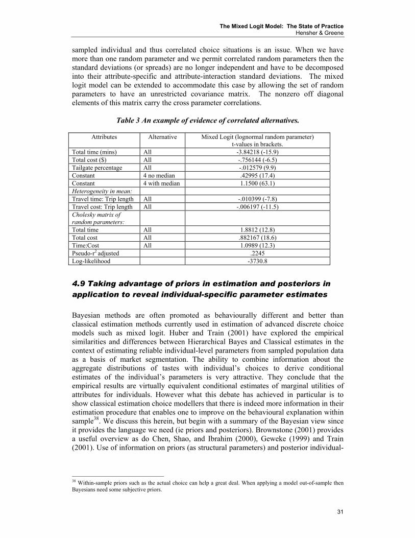
The Mixed Logit Model: The State of Practice Hensher & Greene
31
sampled individual and thus correlated choice situations is an issue. When we have more than one random parameter and we permit correlated random parameters then the standard deviations (or spreads) are no longer independent and have to be decomposed into their attribute-specific and attribute-interaction standard deviations. The mixed logit model can be extended to accommodate this case by allowing the set of random parameters to have an unrestricted covariance matrix. The nonzero off diagonal elements of this matrix carry the cross parameter correlations.
Table 3 An example of evidence of correlated alternatives.
Attributes Alternative Mixed Logit (lognormal random parameter) t-values in brackets.
Total time (mins) All -3.84218 (-15.9) Total cost ($) All -.756144 (-6.5) Tailgate percentage All -.012579 (9.9) Constant 4 no median .42995 (17.4) Constant 4 with median 1.1500 (63.1) Heterogeneity in mean: Travel time: Trip length All -.010399 (-7.8) Travel cost: Trip length All -.006197 (-11.5) Cholesky matrix of random parameters:
Total time All 1.8812 (12.8) Total cost All .882167 (18.6) Time:Cost All 1.0989 (12.3) Pseudo-r2 adjusted .2245 Log-likelihood -3730.8
4.9 Taking advantage of priors in estimation and posteriors in application to reveal individual-specific parameter estimates
Bayesian methods are often promoted as behaviourally different and better than classical estimation methods currently used in estimation of advanced discrete choice models such as mixed logit. Huber and Train (2001) have explored the empirical similarities and differences between Hierarchical Bayes and Classical estimates in the context of estimating reliable individual-level parameters from sampled population data as a basis of market segmentation. The ability to combine information about the aggregate distributions of tastes with individual’s choices to derive conditional estimates of the individual’s parameters is very attractive. They conclude that the empirical results are virtually equivalent conditional estimates of marginal utilities of attributes for individuals. However what this debate has achieved in particular is to show classical estimation choice modellers that there is indeed more information in their estimation procedure that enables one to improve on the behavioural explanation within sample38. We discuss this herein, but begin with a summary of the Bayesian view since it provides the language we need (ie priors and posteriors). Brownstone (2001) provides a useful overview as do Chen, Shao, and Ibrahim (2000), Geweke (1999) and Train (2001). Use of information on priors (as structural parameters) and posterior individual-
38 Within-sample priors such as the actual choice can help a great deal. When applying a model out-of-sample then Bayesians need some subjective priors.
The Mixed Logit Model: The State of Practice Hensher & Greene
32
specific parameters estimates from conditional utility functions are included as information to captured sources of heterogeneity39. The key difference between Bayesian and classical statistics is that Bayesians treat parameters as random variables. Bayesians summarise their prior knowledge about parameters θ by a prior distribution, ( )θπ . The sampling distribution, or likelihood function, is given by ( )θ|xf . After observing some data, the information about θ is given by the posterior distribution:
( ) ( ) ( )( ) ( ) ( )∫
=θθπθ
θπθθdxf
xfxp|
|| (17)
All inference is based on this posterior distribution. The optimal Bayes estimator is the mean of the posterior distribution, and Bayesian confidence bands are typically given by the smallest region of the posterior distribution with the specified coverage probability. Bayesian confidence regions are interpreted as fixed regions containing the random parameter θ with the specified coverage probability. This is different from the classical confidence region, which is a region with random endpoints that contain the true value θ with the specified probability over independent repeated realisations of the data (Brownstone 2001). Classical inference therefore depends on the distribution of unobserved realisations of the data, whereas Bayesian inference conditions on the observed data. Bayesian inference is also exact and does not rely on asymptotic approximations. The Bayesian approach also requires the a priori specification of a prior distribution for all of the model parameters. In cases where this prior is summarising the results of previous empirical research, specifying the prior distribution is a useful exercise for quantifying previous knowledge (such as the alternative currently chosen). There are, however, many circumstances where the prior distribution cannot be fully based on previous empirical work, and the resulting specification of prior distributions based on the analyst’s subjective beliefs is the most controversial part of Bayesian methodology. Poirier (1988) argues that the subjective Bayesian approach is the only approach consistent with the usual rational actor model to explain individuals’ choices under uncertainty. More importantly, the requirement to specify a prior distribution enforces intellectual honesty on Bayesian practitioners. All empirical work is guided by prior knowledge and the subjective reasons for excluding some variables and observations are usually only implicit in the classical framework. Bayesians are therefore forced to carry out sensitivity analysis across other reasonable prior distributions to convince others that their empirical results are not just reflections of their prior beliefs (Brownstone 2001). The simplicity of the formula defining the posterior distribution hides some difficult computational problems, explained in Brownstone (2001)40. 39 We capture within the classical estimation framework the same information that Hierarchical Bayes modellers capture. 40 Computing the posterior distribution typically requires integrating over θ , and this can be difficult for the number of parameters frequently encountered in choice modelling. Until recently Bayesians solved this problem by working with conjugate families. These are a family of prior distributions linked to a family of likelihood functions where the posterior distribution is in the same family as the prior distribution. For example, the Beta family is a conjugate prior for the binomial with fixed number of trials. Koop and Poirier (1993) have developed and applied a conjugate prior for the conditional (and multinomial) logit model, but there do not appear to be tractable conjugate priors for other GEV discrete choice models.
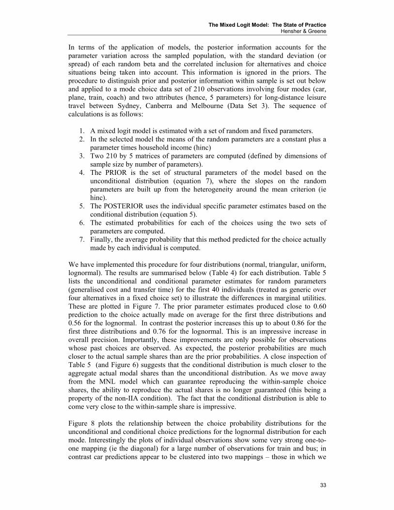
The Mixed Logit Model: The State of Practice Hensher & Greene
33
In terms of the application of models, the posterior information accounts for the parameter variation across the sampled population, with the standard deviation (or spread) of each random beta and the correlated inclusion for alternatives and choice situations being taken into account. This information is ignored in the priors. The procedure to distinguish prior and posterior information within sample is set out below and applied to a mode choice data set of 210 observations involving four modes (car, plane, train, coach) and two attributes (hence, 5 parameters) for long-distance leisure travel between Sydney, Canberra and Melbourne (Data Set 3). The sequence of calculations is as follows:
1. A mixed logit model is estimated with a set of random and fixed parameters. 2. In the selected model the means of the random parameters are a constant plus a
parameter times household income (hinc) 3. Two 210 by 5 matrices of parameters are computed (defined by dimensions of
sample size by number of parameters). 4. The PRIOR is the set of structural parameters of the model based on the
unconditional distribution (equation 7), where the slopes on the random parameters are built up from the heterogeneity around the mean criterion (ie hinc).
5. The POSTERIOR uses the individual specific parameter estimates based on the conditional distribution (equation 5).
6. The estimated probabilities for each of the choices using the two sets of parameters are computed.
7. Finally, the average probability that this method predicted for the choice actually made by each individual is computed.
We have implemented this procedure for four distributions (normal, triangular, uniform, lognormal). The results are summarised below (Table 4) for each distribution. Table 5 lists the unconditional and conditional parameter estimates for random parameters (generalised cost and transfer time) for the first 40 individuals (treated as generic over four alternatives in a fixed choice set) to illustrate the differences in marginal utilities. These are plotted in Figure 7. The prior parameter estimates produced close to 0.60 prediction to the choice actually made on average for the first three distributions and 0.56 for the lognormal. In contrast the posterior increases this up to about 0.86 for the first three distributions and 0.76 for the lognormal. This is an impressive increase in overall precision. Importantly, these improvements are only possible for observations whose past choices are observed. As expected, the posterior probabilities are much closer to the actual sample shares than are the prior probabilities. A close inspection of Table 5 (and Figure 6) suggests that the conditional distribution is much closer to the aggregate actual modal shares than the unconditional distribution. As we move away from the MNL model which can guarantee reproducing the within-sample choice shares, the ability to reproduce the actual shares is no longer guaranteed (this being a property of the non-IIA condition). The fact that the conditional distribution is able to come very close to the within-sample share is impressive. Figure 8 plots the relationship between the choice probability distributions for the unconditional and conditional choice predictions for the lognormal distribution for each mode. Interestingly the plots of individual observations show some very strong one-to-one mapping (ie the diagonal) for a large number of observations for train and bus; in contrast car predictions appear to be clustered into two mappings – those in which we

The Mixed Logit Model: The State of Practice Hensher & Greene
34
have a very high unconditional choice probability (top horizontal profile) in range of 0.78-1.0 which has a conditional spread from 0.05 to 0.9; and those with a very low unconditional choice probability in the range 0 to 0.2 with an equivalent conditional choice probability spread from 0 to 0.85. In the latter case, there is a greater cluster around 0.0 to 0.2 where we have clearly mapped very well (close to the diagonal). These graphs are useful indicators of what information we might seek in an unconditional choice probability in order to move it towards the conditional distribution, given that choice priors are not available for out-of-sample applications (without resort to subjective priors). The graphs suggest that we need to include some additional attributes in the air alternative utility expression to move the horizontal cluster around zero on the unconditional distribution so as to pivot these data points upwards towards the diagonal. By drilling down in the data for these observations compared to the rest of the data one might identify possible additional attributes. The same logic would be applied to the observations on the other alternatives.
Table 4 Average Choice predictions for prior and posterior specifications under alternative distributional assumptions (Sample choice shares: Air = 0.276, Car = 0.281, Bus = 0.143,
Train = 0.300)
Overall Triangular Uniform Normal Lognormal
Prior 0.6062 0.6051 0.6094 0.5633 Posterior 0.8565 0.8709 0.8580 0.7572 Plane Triangular Uniform Normal Lognormal Prior 0.1948 (.329) .207 (.337) .195 (.328) 0.2614 (.314) Posterior 0.2712 (.271) .272 (.385) .274 (.384) 0.2465 (.339) Car Triangular Uniform Normal Lognormal Prior 0.2116 (.294) .202 (.287) .223 (.299) 0.1999 (.227) Posterior 0.2799 (.441) .280 (.441) .280 (.439) 0.2974 (.150) Coach Triangular Uniform Normal Lognormal Prior 0.2054 (.314) .208 (.321) .202 (.311) 0.1742 (.249) Posterior 0.1472 (.299) .148 (.303) .146 (.299) 0.1503 (.255) Train Triangular Uniform Normal Lognormal Prior 0.3881 (.374) .383 (.380) .380 (.373) 0.3645 (.325) Posterior 0.3017 (.387) .299 (.390) .299 (.387) 0.3058 (.348)
The Mixed Logit Model: The State of Practice Hensher & Greene
35
Table 5. List of first 50 conditional and unconditional parameter estimates for
generalised cost and transfer time.
Lognormal Triangular GC GC ttme ttme GC GC ttme ttme
Prior Posterior Prior Postrior Prior Posterior Prior Postrior 0.022794 0.029517 0.129818 0.21678 -0.04093 -0.06942 -0.21598 -0.34837 0.02184 0.027484 0.126588 0.200674 -0.0389 -0.06227 -0.21272 -0.32167 0.023789 0.030458 0.133131 0.221171 -0.04296 -0.06868 -0.21924 -0.34037 0.030745 0.036185 0.154859 0.216953 -0.05514 -0.07307 -0.23883 -0.32256 0.024828 0.032143 0.136528 0.231865 -0.04499 -0.07181 -0.22251 -0.35014 0.02005 0.018678 0.120367 0.107638 -0.03485 -0.02516 -0.20619 -0.15824 0.024828 0.021422 0.136528 0.106915 -0.04499 -0.02238 -0.22251 -0.11666 0.018725 0.025999 0.115611 0.223161 -0.0316 -0.0664 -0.20097 -0.36758 0.023789 0.031042 0.133131 0.225935 -0.04296 -0.07227 -0.21924 -0.35661 0.030745 0.037159 0.154859 0.226897 -0.05514 -0.07844 -0.23883 -0.34736 0.019211 0.025819 0.117372 0.216344 -0.03282 -0.06069 -0.20293 -0.33396 0.022794 0.028236 0.129818 0.200382 -0.04093 -0.06286 -0.21598 -0.31859 0.025913 0.03187 0.140012 0.213312 -0.04702 -0.06892 -0.22577 -0.32725 0.023789 0.029617 0.133131 0.208405 -0.04296 -0.06564 -0.21924 -0.32802 0.021106 0.028264 0.124062 0.219494 -0.03728 -0.06746 -0.21011 -0.35257 0.021106 0.021615 0.124062 0.135449 -0.03728 -0.043 -0.21011 -0.23749 0.021106 0.021898 0.124062 0.139572 -0.03728 -0.043 -0.21011 -0.23678 0.017788 0.018432 0.112167 0.125359 -0.02916 -0.03592 -0.19705 -0.22795 0.02005 0.018137 0.120367 0.102836 -0.03485 -0.02339 -0.20619 -0.15203 0.031276 0.03234 0.156427 0.174549 -0.05595 -0.06029 -0.24013 -0.26071 0.017788 0.018469 0.112167 0.126231 -0.02916 -0.03598 -0.19705 -0.22916 0.018407 0.017379 0.114451 0.105134 -0.03079 -0.02076 -0.19966 -0.15278 0.025913 0.016308 0.140012 0.060105 -0.04702 0.005206 -0.22577 0.020603 0.025913 0.02156 0.140012 0.10154 -0.04702 -0.01372 -0.22577 -0.06874 0.01971 0.020435 0.11916 0.134772 -0.03403 -0.03432 -0.20489 -0.20605 0.028226 0.02863 0.147248 0.15885 -0.05108 -0.05245 -0.2323 -0.23896 0.024828 0.017578 0.136528 0.07239 -0.04499 0.001354 -0.22251 0.002496 0.01971 0.018402 0.11916 0.108326 -0.03403 -0.02212 -0.20489 -0.14879 0.018095 0.015602 0.113303 0.08779 -0.02998 -0.00909 -0.19836 -0.10106 0.017788 0.018612 0.112167 0.128989 -0.02916 -0.0361 -0.19705 -0.22922 0.02005 0.02127 0.120367 0.143487 -0.03485 -0.04145 -0.20619 -0.23589 0.024828 0.025555 0.136528 0.151345 -0.04499 -0.05014 -0.22251 -0.24774 0.030745 0.025856 0.154859 0.114096 -0.05514 -0.03739 -0.23883 -0.15728 0.017487 0.018631 0.111042 0.133189 -0.02835 -0.03564 -0.19575 -0.23051 0.023789 0.024626 0.133131 0.150239 -0.04296 -0.04953 -0.21924 -0.24977 0.022794 0.023938 0.129818 0.15047 -0.04093 -0.04685 -0.21598 -0.24367 0.023789 0.021273 0.133131 0.110608 -0.04296 -0.0308 -0.21924 -0.16378 0.017487 0.017632 0.111042 0.116544 -0.02835 -0.02722 -0.19575 -0.1911 0.019211 0.016772 0.117372 0.093467 -0.03282 -0.01421 -0.20293 -0.1164 0.021106 0.020208 0.124062 0.118668 -0.03728 -0.02556 -0.21011 -0.15466

The Mixed Logit Model: The State of Practice Hensher & Greene
36
Generalised Cost Distributions (Lognormal)
0
0.005
0.01
0.015
0.02
0.025
0.03
0.035
0.04
1 3 5 7 9 11 13 15 17 19 21 23 25 27 29 31 33 35 37 39
Individual Observations
PriorPosterior
Transfer Time Distribution (Lognormal)
0
0.05
0.1
0.15
0.2
0.25
1 3 5 7 9 11 13 15 17 19 21 23 25 27 29 31 33 35 37 39
Individual observations
PriorPostrior
Figure 7. Comparison of the Unconditional (prior) and conditional (posterior)
parameter estimates for random parameters

The Mixed Logit Model: The State of Practice Hensher & Greene
37
Air Train
PROBPR
.0
.2
.4
.6
.8
1.0
1.2
-.2.0 .2 .4 .6 .8 1.0 1.2-.2
PRO
BPO
PROBPR
.0
.2
.4
.6
.8
1.0
1.2
-.2.0 .2 .4 .6 .8 1.0 1.2-.2
PRO
BPO
Bus Car
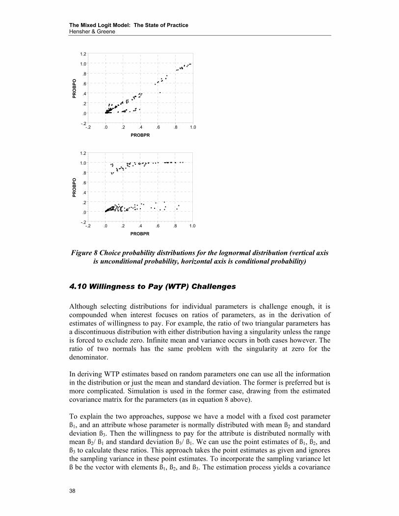
The Mixed Logit Model: The State of Practice Hensher & Greene
38
PROBPR
.0
.2
.4
.6
.8
1.0
1.2
-.2.0 .2 .4 .6 .8 1.0-.2
PRO
BPO
PROBPR
.0
.2
.4
.6
.8
1.0
1.2
-.2.0 .2 .4 .6 .8 1.0-.2
PRO
BPO
Figure 8 Choice probability distributions for the lognormal distribution (vertical axis
is unconditional probability, horizontal axis is conditional probability)
4.10 Willingness to Pay (WTP) Challenges
Although selecting distributions for individual parameters is challenge enough, it is compounded when interest focuses on ratios of parameters, as in the derivation of estimates of willingness to pay. For example, the ratio of two triangular parameters has a discontinuous distribution with either distribution having a singularity unless the range is forced to exclude zero. Infinite mean and variance occurs in both cases however. The ratio of two normals has the same problem with the singularity at zero for the denominator. In deriving WTP estimates based on random parameters one can use all the information in the distribution or just the mean and standard deviation. The former is preferred but is more complicated. Simulation is used in the former case, drawing from the estimated covariance matrix for the parameters (as in equation 8 above). To explain the two approaches, suppose we have a model with a fixed cost parameter ß1, and an attribute whose parameter is normally distributed with mean ß2 and standard deviation ß3. Then the willingness to pay for the attribute is distributed normally with mean ß2/ ß1 and standard deviation ß3/ ß1. We can use the point estimates of ß1, ß2, and ß3 to calculate these ratios. This approach takes the point estimates as given and ignores the sampling variance in these point estimates. To incorporate the sampling variance let ß be the vector with elements ß1, ß2, and ß3. The estimation process yields a covariance

The Mixed Logit Model: The State of Practice Hensher & Greene
39
matrix for all the estimated parameters. One extracts the part for ß (call it W), which is a 3 by 3 symmetric matrix. We now wish to draw random observations from the normal distribution which has mean β and covariance matrix W. The Cholesky decomposition provides a convenient way to do so. The matrix W is decomposed into the product LL′ where L is a lower triangular matrix. Then, the sample we seek can be drawn by first obtaining a set of 3 independent standard normal draws in a vector u, which is simple since the 3 draws can be drawn independently. Then, the desired vector is computed as β + Lu. Thus, we generate draws of ß1, ß2, and ß3 as β
^ +Lu where u is a three by one
vector of IID standard normal deviates drawn from a random number generator and β^
is the point estimate of ß. For each draw, calculate ß2/ ß1 and ß3/ ß1, which are the mean WTP and the standard deviation in WTP implied by those draws. Do this for many draws. Then calculate the mean and standard deviation of ß2/ ß1 over these draws. That gives you the estimated mean WTP and the standard error in this estimated mean. Also calculate the mean and standard deviation of ß3/ ß1 over these draws to get the estimated standard deviation of WTP and the standard error of this estimate. To accommodate the entire distribution of WTP (rather than just the mean and standard deviation), take a draw of ß1, ß2, and ß3 as described above (as β
^ +Lu). For this draw,
one takes numerous draws of WTP, with each draw constructed as (ß2 + ß3*u)/ ß1 where u is a standard normal deviate from a random number generator. Repeat for many draws of ß1, ß2, and ß3, to get many sets of draws of WTP. Then, you can calculate whatever you want to know about WTP from the combined set of WTP draws; e.g., you can calculate the probability that WTP exceeds some amount. Equation (8) above uses this method which we implement below. Using the four lane data for car drivers (Data Set 1) we estimated three models (Table 6) and report the VTTS outputs using the formulae in equation (8). The first model treats travel time as a random parameter, the second model treats travel cost as a random parameter, and the third model allows both travel time and cost to have random parameters. The random parameters are assumed to be correlated in the third model and hence the Cholesky decomposition is used to identify the standard deviations (or spread)41. A lognormal distribution was imposed on all random parameters with sign reversal of the attributes associated with these parameters. The VTTS distributions produce quite different means and standard deviations. For the full sample they range from a mean of $4.773 for travel cost as a random parameter to $5.762 for travel time as a random parameter and $23.4 when both time and cost are random parameters. Since the lognormal distribution has a very long tail (see Table 7), it is often suggested that the last few percentiles could be removed to at least ensure that the mean is a better representation of the majority of the individuals (recognising this unfortunate feature of
41 In order to allow for correlation between the parameters, we would write the entire vector of correlated parameters βi = βmean + ΓΣvi where vi is the set of random draws from the assigned distribution (note, these need not be the same for all parameters), Σ is the diagonal matrix of scale (or “spread”) factors that appears above, and Γ is the lower triangular Cholesky factor of the correlation matrix of the parameters. (Thus, the diagonal elements of Γ are equal to one.) Then, the actual covariance matrix of the random terms that enters the parameters is ΓΣSΣΓ′ where S is diagonal matrix with diagonal elements equal to 1.0 for normally distributed parameters, √6 for uniformly distributed parameters, and √3 for the triangularly distributed parameters. In this case, it can be seen that each parameter is equal to its mean plus a mixture of the random terms which enter some or all of the other parameters. (Since Γ is triangular and Σ is diagonal, βi1 is a function of v1 only, βi2 is a function of vi1 and vi2 and so on.) This allows the parameters to be freely correlated and have an unrestricted scale as well while insuring that the covariance matrix that we estimate is positive definite at all times.

The Mixed Logit Model: The State of Practice Hensher & Greene
40
a lognormal). When we remove the highest two percentile, the mean and standard deviation change significantly, especially for the model with two random parameters (compare Figures 9 and 10). The authors’ experience with a number of data sets suggests a phenomenon that is not unique to a specific data set but widespread. It is not until one investigates the WTP outputs that the critical influence of the actual distributions is highlighted42. Armstrong et al (2001) discuss this issue in the context of confidence intervals.
Table 6 Three Mixed Logit Models with Alternative Random Parameters for WTP calculation.
T-values in brackets. parameters with an asterisk are from the Cholesky matrix. (Data Set 1).
Attributes Alternative Mixed Logit (lognormal random parameter)
M1 (time =RP)
M2 (cost = RP)
M3 (time and cost = RP)
Total time (mins) All -4.7136 (-7.67) -.004874 (-6.4) -3.84218 (-15.9) Total cost ($) All -.12743 (-49.1) -.9469 (-7.3) -.756144 (-6.5) Tailgate percentage All -.010856 (-9.0) -.012145 (-9.7) -.012579 (-9.9) Constant 4 no
median .3199 (13.2) .4117 (16.7) .42995 (17.4)
Constant 4 with median
.9418 (53.2) 1.1213 (61.3) 1.1500 (63.1)
Heterogeneity in mean:
Travel time: Trip length
All -.0061335 (-2.4) - -.010399 (-7.8)
Travel cost: Trip length
All - -.054599 (-9.9) -.006197 (-11.5)
Std Deviation. of parameter distribution
Total time All 1.4876 (7.35) - 1.8812 (12.8)* Total cost All - 1.2578 (15.5) .882167 (18.6)* Time:Cost All - - 1.0989 (12.3)* Pseudo-r2 adjusted .1526 .2152 .2245 Log-likelihood -4078.3 -3776.9 -3730.8 Value of Travel Time Savings ($ per person hour) based on full sample of 4384 observations MLVOTT All 5.762 (20.7) MLVOTC All 4.773 (11.542) MLVOTTC All 23.463 (320.0) Value of Travel Time Savings ($ per person hour) based on truncated sample post-estimation (removing last 2 percentile): MLVOTT All 4.066 (6.72) MLVOTC All 4.0247 (6.25) MLVOTTC All 9.087 (22.4)
42 This is not to suggest that it is an unimportant issue for prediction.

The Mixed Logit Model: The State of Practice Hensher & Greene
41
Kernel density estimate for MLVOTT
MLVOTT
.00
.01
.02
.03
.04
.05
-.010 500 1000 1500-500
Den
sity
Kernel density estimate for MLVOTC
MLVOTC
.000
.025
.050
.075
.100
.125
-.0250 100 200 300 400 500-100
Den
sity
Kernel density estimate for MLVOTTC
MLVOTTC
.180
.384
.588
.793
.997
-.0240 5000 100001500020000 250003000035000-5000
Den
sity
(X10
^-4)
1.1.1.1.1 Figure 9. Full sample distribution of VTTS
1.1.1.1.2 Table 7 Full Sample cumulative distribution of value of travel time savings
Sample Size: 16 choice situations per individual times 274 individuals times 3 alternatives Range ($/person hour) MLVOTT MLVOTC MLVOTTC 0-1 .3897 .3352 .4450 1.01-2 .5605 .5300 .5601 2.01-3 .6577 .6461 .6247 3.01-4 .7237 .7165 .6706 4.01-5 .7673 .7687 .7007 5.01-6 .8006 .8082 .7288 6.01-7 .8225 .8390 .7505 7.01-8 .8429 .8593 .7679 8.01-9 .8597 .8761 .7834 9.01-10 .8733 .8910 .7967 10.01-15 .9196 .9356 .8410 15.01-20 .9441 .9583 .8681 20.01-50 .9840 .9916 .9338 50.01-100 .9949 .9980 .9637 100.01-200 .9989 .9995 .9803 200.02-300 .9993 .9998 .9879 300.01-400 .9995 1.000 .9916 400.01-500 .9997 .9942 500.01-1000 1.000 .9973 Over 1000 1.000

The Mixed Logit Model: The State of Practice Hensher & Greene
42
Kernel density estimate for MLVOTT
MLVOTT
.000
.025
.050
.075
.100
.125
.150
.175
-.0250 10 20 30 40 50 60-10
Den
sity
Kernel density estimate for MLVOTC
MLVOTC
.000
.025
.050
.075
.100
.125
.150
.175
-.0250 10 20 30 40 50 60-10
Den
sity
Kernel density estimate for MLVOTTC
MLVOTTC
.00
.01
.02
.03
.04
.05
.06
.07
-.010 50 100 150 200 250-50
Den
sity
1.1.1.1.3 Figure 10 Removing last two percentile The concern with arbitrarily removing part of a distribution for whatever reason43 suggests a serious consideration of constrained distributions. To illustrate the implications of imposing a constraint on the lognormal distribution we have estimated a series of models using Data Set 4. We have constrained the standard deviation to be 0.75, 1.0, 1.5 and 2.0 of the mean44. The results are summarised in Table 8 (using equation (8)) and Figure 11. The distributions still have a long tail with mean estimates of VTTS declining (from 19.09 to 15.08) as we move from 0.75 of the mean to twice the mean45. This initially might seem odd given that a more constrained standard deviation should reduce the mean; however this is only correct if the distribution is in the numerator. The calculation of VTTS herein uses the cost variable as the random parameter (ie the denominator), and hence the result is as expected. What is particularly noticeable is that the mean estimate of the random parameter increases substantially to almost compensate for the constrained standard deviation, resulting in far less of an impact on the overall average VTTS. While we are capable of imposing such a series of constraints, there appears to be no strong theoretical basis for doing so. Distributions are analytical constructs however and hence the imposition of such constraints is no better or worse than an unconstrained distribution unless there is a theoretical/behavioural rationale. Except for the sign of the WTP, we appear to have no theoretical arguments to support one distribution over another. Practitioners are likely to remain sceptical of WTP measures based on such long tails as typified by the lognormal. The alternative may well be greater consideration of segmentation of attributes in order to establish a discrete set of fixed parameters along a line (essentially points on an undefined distribution). The disadvantage of this is that one might select the set of thresholds and
43 For the normal, uniform and triangular, the negative region for VTTS is often quite substantial, indeed often exceeding 2 percentiles. 44 When you allow for correlation amongst attributes, the scale factor is not the standard deviation of the distribution, even in the normal distribution case. The standard deviation is the square root of the sum of squares of the elements in a row of the Cholesky matrix, and there is no way to make that square root equal to one of the parameters. 45 A referee expected the mean VTTS to equal the standard deviation VTTS when the scale equals unity. This is incorrect since the scale equality is on the first two moments of the travel time parameter.

The Mixed Logit Model: The State of Practice Hensher & Greene
43
segment criteria that are inadequate representations of the heterogeneity in the variance structure of the unobserved effects.
1.1.1.1.4 Table 8 Implications of constrained lognormal distributions on value of travel time savings ($ per driver hour) (2,976 observations)
VTTS distribution Mean Standard
distribution minimum maximum Goodness of Fit
unconstrained 12.60 19.67 0.18 462.7 -740.61 SD=0.75 of mean 19.09 22.09 0.61 420.59 -761.54 SD=mean 18.68 25.13 0.40 533.58 -750.59 SD=1.5 of mean 15.57 23.10 0.26 525.14 -745.51 SD=2.0 of mean 15.08 25.31 0.18 623.99 -742.79
Kernel density estimate for VOTLC
VOTLC
.00
.01
.02
.03
.04
.05
.06
-.010 25 50 75 100 125 150 175-25
Den
sity
Kernel density estimate for VOTLC25
VOTLC25
.000
.025
.050
.075
.100
.125
.150
.175
-.0255 10 15 20 250
Den
sity
Kernel density estimate for VOTLC75
VOTLC75
.000
.005
.010
.015
.020
.025
.030
.035
-.0050 100 200 300 400 500-100
Den
sity
Kernel density estimate for VOTLC1
VOTLC1
.000
.005
.010
.015
.020
.025
.030
.035
-.0050 100 200 300 400 500 600-100
Den
sity
Kernel density estimate for VOTLC15
VOTLC15
.000
.005
.010
.015
.020
.025
.030
.035
.040
-.0050 100 200 300 400 500-100
Den
sity
Kernel density estimate for VOTLC2
VOTLC2
.000
.005
.010
.015
.020
.025
.030
.035
.040
-.0050 50 100 150 200 250 300-50
Den
sity
1.1.1.1.5 Figure 11 Constrained Distributions Relative to unconstrained
distribution (VOTLC)

The Mixed Logit Model: The State of Practice Hensher & Greene
44
To investigate the implications of constraints on other distributions than the lognormal, we estimated a model using the triangular distribution imposing constraints on the spread. Setting the spread to 1.0 guarantees all the same sign. Any other value will lead to both signs. The reason is as follows. Define as before ßi + scaleßit where t is the triangular distribution that ranges from -1 to +1. If the scale equals 1.0, the range is 0 to 2 ß1. We found that the mean VTTS for spread equal to 1.0 is $7.62 (with a range $4.93 to $14.1). Thus the entire distribution is within the positive VTTS range in contrast to the unbounded spread with a mean of $2.51 and a range from -$5848 to $3112 (although 99% of values are in the range -$200 to $240). Figure 12 graphs these two distributions. We conclude on the basis of this evidence that a lower bounded triangular distribution has appeal in that it eliminates the long tail common to a lognormal while ensuring the behaviourally correct sign of WTP. This initial inquiry into constrained distributions suggests a major topic for ongoing research46.
Kernel density estimate for VOTLC1
VOTLC1
.00
.05
.10
.15
.20
.25
.30
-.056 8 10 12 14 164
Den
sity
Kernel density estimate for VOTLC
VOTLC
.000
.005
.010
-.005-5000 0 5000-10000
Den
sity
Figure 12. The VTTS distribution with and without the lower bound for the
triangular distribution. 5. Conclusions The continuing challenges we face with mixed logit models are derived in the main from the quality of the data. Mixed logit certainly demands better quality data than MNL since it offers an extended framework within which to capture a greater amount of true behavioural variability in choice making. It is, broadly speaking, aligning itself much more with reality where every individual has their own inter-related systematic and random components for each alternative in their perceptual choice set(s). Although there is a level of irreducible variability in everyone, its does have some basis in the fact that individuals do not do the same thing all the time for a variety of reasons that analysts cannot fully observe or explain (and probably neither can the individuals themselves). As discrete choice models become less restrictive in their behavioural assumptions, the possibility of identifying sources of heterogeneity associated with the mean and variance of systematic and random components increases. Ultimately we want to improve on our modelling capability to improve the predictability of a model when
46 There are a number of views in the research community about ways of handling the information in distributions. These include using only the mean from a lognormal instead of the simulated distribution and selecting a more symmetrical distribution such as the triangular but constraining it to the non-negative range (as we have done in the text). The evidence herein suggests little gain from constraining a lognormal distribution; however promoting the use of only the mean (including any parameterisation of heterogeneity around the mean) from a lognormal is controversial since relevant information is being discarded. The possibility of eliminating the extreme values where they are small in number remains appealing if one wishes to use a lognormal.

The Mixed Logit Model: The State of Practice Hensher & Greene
45
individuals are faced with changes in the decision environment as represented by a set of attributes of alternatives, characteristics of decision makers and other contextual effects (which can include task complexity for data collection, especially stated choice experiments). The sources of explanatory power reside within the systematic and random components in potentially complex ways and can be captured by both the mean and the variance of parameters representing observed and unobserved effects. The mixed logit model certainly opens up new opportunities to research these behavioural phenomena. What is important for modellers is the recognition that each individual's random component variance is perfectly confounded with their mean or systematic components (Louviere et al 2002). Thus, one needs extra information in order to achieve identification. It is an important and open question as to what that might be in a modelling setting where we abstract from reality to varying degrees and impose additional translation constraints in order to obtain preference and choice responses from individuals. These constraints include the actual design of the data collection instrument and how this relates to the complexity of the choice task that intervenes in the decision making process. Recent work by DeShazo and Fermo (2001), Swait and Adamowicz (2001) amongst others suggests that some individual differences can be used to put structure on the differences in variability. There is always more research required, but at various junctures in the process it is prudent to take stock of progress and to highlight the major developments and warn about the continuing challenges. This paper has set itself this objective in the very specific context of the application of the mixed logit model. A number of very practical issues discussed herein should assist analysts as they venture more into the practical detail of specifying, estimating, and interpreting mixed logit models and in applying their behavioural outputs. Acknowledgements We are indebted to Ken Train for the many hours we have discussed the challenges facing modellers estimating mixed (or random parameter) logit models. Jordan Louviere, David Brownstone and David Bunch also provided a platform to test ideas. Chandra Bhat provided informative comments on an earlier draft. The very extensive comments of three referees are greatly appreciated. The effort each referee made to assist the authors has materially improved this paper. References Armstrong, P., Garrido, R. and Ortuzar, J. deD (2001) Confidence intervals to bound the value of time, Transportation Research 37E (2/3), 143-161. Ben-Akiva, M. and D. Bolduc (1996) Multinomial probit with a logit kernel and a general parametric specification of the covariance structure. Working paper, Department of Civil and Environmental Engineering, MIT Bhat, C.R. (2000) Flexible model structures for discrete choice analysis, in Hensher, D.A. and Button, K. J. (eds) Handbook of Transport Modelling, Volume 1, of Handbooks in Transport, Pergamon Press, Oxford, 71-90.

The Mixed Logit Model: The State of Practice Hensher & Greene
46
Bhat, C. R. (2001) Quasi-random maximum simulated likelihood estimation of the mixed multinomial logit model, Transportation Research, 35B(7), 677-695. Bhat, C. R. (in press) Simulation estimation of mixed discrete choice models using randomised and scrambled Halton sequences, Transportation Research. Bhat, C.R. and Castelar, S. (2002) A unified mixed logit framework for modeling revealed and stated preferences: formulation and application to congestion pricing analysis in the San Francisco Bay Area, Transportation Research, 36B (7), 593-616. Boersch-Supan, A. and Hajvassiliou, V. (1990) Smooth unbiased multivariate probability simulators for maximum likelihood estimation of limited dependent variable models, Journal of Econometrics, 58 (3), 347-368. Brownstone, D. (2001) Discrete choice modelling for transportation, in Hensher, D.A. (ed) in Hensher, D.A. (ed.) Travel Behaviour Research: The Leading Edge, Pergamon Press, Oxford, 97-124. Brownstone, D. and K. Train (1999) Forecasting new product penetration with flexible substitution patterns. Journal of Econometrics, 89, 109-129 Brownstone, D., D. S. Bunch, and K. Train (2000) Joint Mixed Logit Models of Stated and Revealed references for Alternative-fuel Vehicles. Transportation Research B, 34, 315-338. Carrasco, J.A. and Ortuzar, J. deD (2002) Review and assessment of the nested logit model, Transport Reviews, 22 (2), 197-218. Chen, M-H., Shao, Q-M and Ibrahim, J. (2000) Monte Carlo Methods in Bayesian Computation, New York, Springer. Daniels, R. and Hensher, D.A. (2000) Valuation of environmental impacts of transportation projects: the challenge of self-interest proximity, Journal of Transport Economics and Policy, 34 (2), May, 189-214. DeShazo, J.R. and G. Fermo (2001) Designing choice sets for stated preference methods: the effects of complexity on choice consistency, Journal of Environmental Economics and Management, forthcoming. Evans, M., N Hastings and B. Peacock (1993) Statistical Distributions, New York, John Wiley and Sons. Geweke, J. F. (1999) Using simulation methods for Bayesian econometric models: inference, development, and communication (with discussion and reply). Econometric Reviews, 18(1), 1-126 Geweke, J., Keane, M. and Runkle, D. (1994) Alternative computational approaches to inference in the multinomial probit model, Review of Economics and Statistics, LXXVI,(4), 609-632.
The Mixed Logit Model: The State of Practice Hensher & Greene
47
Greene, W.H. (2002) Econometric Analysis, 5th edition, Englewood Cliffs, Prentice Hall. Greene, W.H. and Hensher, D.A. (2002) A latent class model for discrete choice analysis: contrasts with mixed logit. Institute of Transport Studies Working Paper ITS-WP-02-08, University of Sydney, April. Halton, J.H. (1960) On the efficiency of certain quasi-random sequences of points in evaluating multidimensional integrals, Numerische Math, 2, 84-90 and corrigenda 196. Hensher, D.A. (2001a) Measurement of the valuation of travel time savings, Journal of Transport Economics and Policy (Special Issue in Honour of Michael Beesley), 35 (1), 71-98. Hensher, D.A. (2001b) The Valuation of Commuter Travel Time Savings for Car Drivers in New Zealand: Evaluating Alternative Model Specifications, Transportation, 28 (2), 101-118. Hensher, D.A. and Johnson, L.W. (1981) Applied Discrete Choice Modelling, Croom Helm (London) and Wiley (New York). Hensher, D.A., Louviere, J.J. and Swait, J. (1999) Combining Sources of Preference Data, Journal of Econometrics, 89, 197-221. Hensher, D.A. and Sullivan, C. (2003) Willingness to pay for road curviness and road type for long distance travel in New Zealand, Transportation Research D. Huber, J. and Train, K. (2001) On the similarity of classical and Bayesian estimates of individual mean partworths, Marketing Letters, 12 (3), August, 259-270. Koop, G. and D. J. Poirier (1993) Bayesian Analysis of Logit Models using Natural Conjugate Priors. Journal of Econometrics, 56, 323-340 Koppelman, F. and Sethi, V. (2000) Closed-form discrete-choice models, in Hensher, D.A. and Button, K. J. (eds) Handbook of Transport Modelling, Volume 1, of Handbooks in Transport, Pergamon Press, Oxford, 211-222. Louviere, J.J. and Hensher, D.A. (2001) Combining sources of preference data, in Hensher, D.A. (ed.) Travel Behaviour Research: The Leading Edge, Pergamon Press, Oxford, 125-144. Louviere, J.J., Hensher, D.A. and Swait, J.F. (2000) Stated Choice Methods and Analysis, Cambridge University Press, Cambridge. Louviere, J., Carson, R., Ainslie, A., Cameron, T., DeShazo, J.R., Hensher, D., Kohn, R., Marley, T., and Street, D. (2002) Dissecting the random component of utility, Workshop Report for the Asilomar Invitational Choice Symposium, California, June (to appear in Marketing Letters).

The Mixed Logit Model: The State of Practice Hensher & Greene
48
McFadden, D. (2001) Disaggregate Behavioural Travel Demand’s RUM Side – A 30 years retrospective in Hensher, D.A. (ed.) Travel Behaviour Research: The Leading Edge, Pergamon Press, Oxford, 17-64. McFadden, D. and Ruud, P.A. (1994) Estimation by simulation, Review of Economics and Statistics, LXXVI,(4), 591-608. McFadden, D. and K. Train (2000) Mixed MNL models for discrete response, Journal of Applied Econometrics, 15, 447-470. Poirier, D. J. (1988) Frequentist and Subjectivist Perspectives on the Problems of Model Building in Economics (with discussion and reply). Journal of Economic Perspectives, 2, 121-170 Revelt, D. & K. Train (1998) Mixed Logit with repeated choices: households' choices of appliance efficiency level, Review of Economics and Statistics, 80, 1-11. Rizzi, L.I and Ortuzar, J. deD. (2002) Stated preference in the valuation of interurban road safety, Accident Analysis and Prevention, Stern, S. (1997) Simulation-based estimation, Journal of Economic Literature, XXXV. December, 2006-2039. Swait, J. and Adamowicz, W. (2001) Choice complexity and decision strategy selection, Journal of Consumer Research, 28, 135-148. Train, K. (1997) Mixed logit models for recreation demand, in Kling, C. and Herriges, J. (eds.) Valuing the Environment Using Recreation Demand Models, Elgar Press, New York. Train, K. (1998) Recreation demand models with taste differences over people. Land Economics, 74(2), 230-239 Train, K. (1999) Halton Sequences for Mixed Logit. Working paper, Department of Economics, University of California, Berkeley. Train, K. (2001) A comparison of hierarchical Bayes and maximum simulated likelihood for mixed logit, Paper presented at the Asilomar Invitational Choice Symposium, California, June. Appendix: Halton Sequences for Monte Carlo Integration
Computation of the choice probabilities in equation (6) typically requires Monte Carlo integration. The computation involves the generation of pseudo-random sequences intended to mimic independent draws from a uniform distribution on the unit interval. Although these pseudo-random sequences cannot be distinguished from draws from a uniform distribution, they are not spread uniformly over the unit interval.

The Mixed Logit Model: The State of Practice Hensher & Greene
49
Bhat (2000, 2001) however has shown that an alternative quasi-random maximum simulated likelihood method (known as Halton Sequences (after Halton 1960)) which uses non-random more uniformly distributed sequences instead of pseudo-random points provides greatly improved accuracy with far fewer draws and computational time. These sequences yield more accurate approximations in Monte Carlo integration relative to standard pseudo-random sequences (Brownstone 2001). The reason for the superior performance of these sequences is shown in Figure 1 (from Bhat (2001)). Even with 1,000 draws, the pseudo-random sequences leave noticeable holes in the unit square, while the Halton sequence used by Bhat gives very uniform coverage. Bhat (2001) gives results from a Monte Carlo study of simulated maximum mixed logit models to compare the performance of the Halton sequence and the standard pseudo-random sequence. For four and five dimension integrals the Halton sequence methods required 125 draws to achieve the same accuracy as 2,000 draws with the standard pseudo-random number sequences. As a result, the computation time required to estimate the mixed logit model using Halton sequences was 10% of the time required for the standard methods. Train (1999), Revelt and Train (1999) and Hensher (2001a) have also reported similar large reductions in computation time using Halton sequences for mixed logit estimation. These results clearly demonstrate the promise of these alternative numerical methods for estimating mixed logit models.
1000 Draws on the Unit Square (from Bhat (2001))