The mathematical structure of multiphase thermal · PDF fileThe mathematical structure of multiphase thermal models of ... for modelling multicomponent, two-phase, thermal ﬂuid ﬂow

The mathematical structure of multiphase

thermal models of flow in porous media

By Daniel E.A. van Odyck1,†, John B. Bell2, Franck Monmont3 and

Nikolaos Nikiforakis1

1Department of Applied Mathematics and Theoretical Physics, University of

Cambridge, Cambridge CB3 0WA, UK2Lawrence Berkeley National Lab, Berkeley, CA 94720, USA

3Schlumberger Cambridge Research, Cambridge CB3 0EL, UK

This article is concerned with the formulation and numerical solution of equationsfor modelling multicomponent, two-phase, thermal fluid flow in porous media. Thefluid model consists of individual chemical component (species) conservation equa-tions, Darcy’s law for volumetric flow rates and an energy equation in terms ofenthalpy. The model is closed with an equation of state and phase equilibrium con-ditions that determine the distribution of the chemical components into phases. Itis shown that, in the absence of diffusive forces, the flow equations can be splitinto a system of hyperbolic conservation laws for the species and enthalpy and aparabolic equation for pressure. This decomposition forms the basis of a sequentialformulation where the pressure equation is solved implicitly and then the com-ponent and enthalpy conservation laws are solved explicitly. A numerical methodbased on this sequential formulation is presented and used to demonstrate sometypical flow behaviour that occurs during fluid injection into a reservoir.

Keywords: porous media flow, multiphase flow, multicomponent flow, phase

equilibrium, conservation laws

1. Introduction

This article is concerned with the mathematical formulation and numerical solutionof systems of partial differential equations for multicomponent, two phase flow inporous media that include thermal effects. The latter are important in the numer-ical simulation of enhanced oil recovery processes such as steam flooding and in

situ combustion. Relevant methodologies have been reported in recent papers byLiu et al. (2007), Huang et al. (2007), Pasarai et al. (2005), Nilsson et al. (2005)and Christensen et al. (2004). Thermal process simulation also plays an importantrole in the modelling of geothermal reservoirs (the reader is referred to the recentsurvey by O’Sullivan et al. 2001). Modelling the behaviour and evaluating cleanupstrategies for contaminants can also require the treatment of thermal processes, seefor example Class et al. (2002) and the references cited therein for a survey of thistype of application.

The development of solution methodologies for the simulation of complex sub-surface thermal processes often leads to a compromise between accuracy and stabil-

† Author for correspondence ([email protected])

Article submitted to Royal Society TEX Paper

2 D.E.A. van Odyck et al.

ity. Many of these thermal processes are characterised by sharp fronts propagatingthrough the medium, which places stringent requirements on spatial and temporalresolution. However, the simulations also rely on an accurate coupling of a numberof different processes, which places stringent requirements on process coupling andstability. The trend in recent years has been to place an emphasis on stability ratherthan spatial accuracy. Consequently, most approaches to thermal simulations arebased on a fully-implicit formulation with lower-order implicit spatial differencing.Most of the approaches in the literature cited above are based on this type of strat-egy. It is also worth mentioning the work of Christensen et al. (2004) and Nilssonet al. (2005), who utilise adaptive mesh techniques to improve spatial resolution.

The goal of the present work is to develop an algorithm for modelling multi-phase, multicomponent non-isothermal reacting flows that achieves a better balancebetween stability and accuracy. As part of this development, we will examine themathematical structure of these types of flows which provides the basis for apply-ing contemporary high-resolution upwind methodology in this context. Examplesof this type of approach for the black-oil model are discussed in Bell et al. (1989).Similar types of discretization procedures are considered for compositional modelsin Mallison et al. (2003).

The approach taken here was used previously to analyse the structure of black-oil(Trangenstein & Bell 1989a) and compositional (Trangenstein & Bell 1989b) mod-els for reservoir simulation. It represents a generalisation of the classical derivationof the Buckley-Leverett equation, see for example Peaceman (1977). As in the de-velopment of compositional models by Trangenstein & Bell (1989b) the followinganalysis relies heavily on the mathematical structure of the multiphase multicom-ponent phase behaviour. The treatment of phase behaviour for non-isothermal sys-tems using an optimisation framework is discussed in Brantferger (1991a) as part ofthe development of a fully implicit thermal-compositional solver and in Michelsen(1999).

The rest of the paper is structured as follows. In section 2, we review the ba-sic equations for multiphase, non-isothermal flow in porous media and discuss thestructure of the phase equilibrium problem. In section 3 the sequential splitting ofthe flow equations is introduced. This sequential form separates the system into aparabolic pressure equation and a system of conservation laws for the chemical con-stituents of the fluid and the enthalpy of the rock / fluid system. We show in section4 that, in the absence of capillary pressure and diffusive transport, this system ofconservation laws is hyperbolic. We develop a numerical algorithm based on thisformulation in section 5. Finally we present numerical results based on the sequen-tial formulation that illustrate the behaviour of the interacting waves encounteredin the system. These examples serve to validate the sequential formulation andillustrate the types of wave behaviour associated with this type of system.

2. Mathematical formulation

In this section, we present the basic flow equations describing non-isothermal, mul-tiphase, multicomponent flows in heterogeneous porous media. The porosity of themedium is denoted by φ, and the phase volume of each phase per pore volume isdenoted uα. Greek subscripts refer to mobile phases. (The medium itself, which canbe viewed as a solid phase is given a distinguished treatment since it is immobile.)

Article submitted to Royal Society

Mathematical structure porous media flow 3

The multicomponent mixture is composed of N components (or lumped pseudo-components) and we define nα as the vector of moles of each component in phaseα divided by the pore volume. Thus,

∑

α nα ≡ n is the total number of moles perpore volume of these components in the combined fluid system. (Mineral contentof the solid is, of course, important for geochemistry but is not included in thesedefinitions.)

Flow equations

The flow is governed by the equations of mass and energy conservation and byDarcy’s law, which gives the volumetric flow rate, ~vα, of each phase in terms of thephase pressure, pα

~vα = −Kkr,α

ηα

(∇pα − ρα~g) ≡ −λα(∇pα − ρα~g) (2.1)

where K is the permeability of the medium, kr,α is the relative permeability, whichexpresses the modification of the flow rate from multiphase effects, ηα and ρα arethe phase viscosity and density, respectively, and ~g is the gravitational force. Hereλα ≡ Kkr,α/ηα is the phase mobility. The pressure in each phase is related to areference pressure, p (typically taken to be the most wetting phase), by a capillarypressure, pc,α = pα − p, which is a function of saturation.

Conservation of mass for each component is given by

∂(φn)

∂t+ ∇ ·

∑

α

nα

uα

~vα = ∇ ·D + Rn (2.2)

Here D are diffusive terms that include multiphase molecular diffusion and disper-sion and Rn are reaction terms. Both the diffusion and reaction terms can be quitecomplex, depending on the particular problem, see for example Chen et al (2006)for a detailed discussion of these terms.

For non-isothermal systems it is necessary to include the energy conservationin the system of equations. The overall energy balance must include energy in thesolid phase. If we assume that the porous medium and the fluids are in thermalequilibrium, the energy balance is of the form

∂Ht

∂t+ ∇ ·

∑

α

~vα

uα

nαThα = ∇ · ~q + RH , (2.3)

where Ht = (1 − φ)ρrHr + φ∑

α nαThα is the total enthalpy of the system, hα

are the partial molar phase enthalpies, Hr the enthalpy of the medium and ρr

the density of the medium. Here ~q represents diffusive energy transport processessuch as thermal conduction and RH represents energy release from reactions andexternal heating. If one does not assume the porous medium and the fluid arein thermal equilibrium, RH will contain relaxation terms that equilibrate the twotemperatures. In the above formulation we have omitted a term from the right handside of the form

∂∑

α pαuα

∂t+∑

α

~vα · ∇pα .



Omitting this term implicitly assumes that the change in phase pressures is slowso that these terms can be ignored. We note that formulations based on internalenergy make a similar assumption by dropping a term of the form

∑

α

~vα · ∇pα

from the energy equation. For a more detailed derivation and discussion, the readershould refer to Burger et al (1985).

Phase behaviour

The component conservation and energy equations express the change in totalmass of each component due to advection, diffusion and chemical reactions. Sincecomponents are being transported in phases, it is necessary to know the compositionof the phases before we can solve the flow equations. This decomposition is referredto as the phase behaviour of the system. The phase behaviour is determined bysaying that the equilibrium state of the mixture occurs at the point of maximumentropy. The entropy of the phases is derived from the chemical potential µα. Thesechemical potentials are typically specified in terms of an equation of state to modelthe dependence of pressure on temperature, composition and specific volume ofthe phase. For a more detailed discussion see Michelson & Mollerup (2004) andBrantferger et al. (1991b).

The chemical potentials µα are functions of pα, T , and phase composition nα.Note that we have preserved the role of capillary pressure in determining the ther-modynamic behaviour of the system. One simplification is to define the thermody-namics in terms of the reference pressure and retain capillary pressure effects onlyin the definition of phase velocities, see Brantferger et al. (1991b). Furthermorethe major thermodynamic variables describing each phase can all be expressed interms of the phase’s chemical potential. In particular, the partial molar entropiesare given by

sα = −(

∂µα

∂T

)

xα,pα

(2.4)

where xα = nα/eTnα are the mole fractions, e = (1, 1, .., 1)T , and the partial molar

enthalpies are given by

hα = (µα + T sα) . (2.5)

Here the phase equilibrium problem is to determine the composition of thephases nα given the total moles n, pressure P and the total enthalpy Ht. Theequilibrium distribution of the components is given by minimising the negativeentropy of the system. In a two-phase liquid and vapour case this becomes

min[

−S = −(nTl sl + n

Tv sv)

]

subject to

n = nl + nv

and

Ht = (1 − φ)ρrhr + φ(nTl hl + n

Tv hv)



along with inequality constraints (nα ≥ 0) guaranteeing non-negativity of the com-positions and thermal stability of the fluid (nα

T ∂hα

∂T> 0). As noted above, if we do

not consider the solid and the fluids to be in thermal equilibrium then we hold thetotal fluid enthalpy, Hf = n

Tl hl + n

Tv hv, constant rather than the total enthalpy.

Treatment of this minimisation problem, i.e. the so-called isenthalpic flash calcu-lation, has been presented in the literature (Michelsen & Mollerup (2004); Michelsen(1999); Brantferger (1999a)) and will not be discussed in detail here. There are,however, a couple of key observations about the structure of the minimisation thatwill play a role later in the development of the sequential discretization. Firstly,the Hessian of the negative entropy is a rank one perturbation of the Hessian ofthe Gibbs free energy, which is minimised in an isothermal flash calculation. Con-sequently, it is computationally simple to compute one of theses matrices given theother. Secondly, at equilibrium the chemical potentials are equal, i.e.,

1

Tµl(xl, T, pl) =

1

Tµv(xv, T, pv) (2.6)

Here, the chemical potentials are typically specified in terms of mole fractions ratherthan moles; however, we can use the definition of mole fractions to express them inthis form.

In addition to determining the composition of the phases and the temperature,the phase behaviour also determines the properties of the phases. In particular,given pressure, temperature and component mass densities, we can compute thevolume occupied by the phases. To complete the mathematical formulation of thesystem we require that the sum of the phase volumes match the available porevolume, which we will represent as

1 = U(p, T,n) =∑

α

uα(pα, T,nα) . (2.7)

This equation plays the role of an equation of state that constrains the evolutionof the component conservation and energy equations. Here we have implicitly usedthe capillary pressure to relate the phase pressures to the reference pressure.

3. The sequential formulation

In this section we present a sequential formulation of the above thermal / compo-sitional model. This approach, based on a total velocity splitting with a pressureequation determined by differentiating the equation of state (2.7) was first intro-duced by Acs & Dolschal (1985). The methodology introduced here follows thedevelopment in Trangenstein & Bell (1989b) and, as such, represents a generalisa-tion of that work to a non-isothermal setting. As in Brantferger (1991a), we willuse pressure, total enthalpy and molar densities as the primary unknowns. The useof enthalpy as a primary unknown instead of temperature reflects its role as theconserved variable in the energy equation. This choice also avoids issues related tothe Gibbs phase rule that can occur if there are more phases than components, inwhich case pressure and temperature cannot vary independently. However, it alsointroduces some complexity because many of the thermodynamic variables are givenin terms of the temperature, T . In particular, the functional form of the enthalpy



is given by

Ht = Ht(n, T, p) . (3.1)

We view this relationship as implicitly defining the temperature as a function ofthe molar densities, pressure and the enthalpy. We also note that for some of theanalysis it will be convenient to derive an equation for temperature; however, inthe numerical method, the enthalpy is the quantity that is advanced in time.

Formally, the dynamics evolves conservation equations for the chemical compo-nents and energy with phase velocities given by Darcy’s law. The entire evolutionis constrained by the equation of state.

Pressure equation

As in Acs & Dolshal (1985) and Trangenstein & Bell (1989b), we first derivea pressure equation to satisfy the total volume balance by taking the first orderTaylor expansion in time of the pore volume constraint (equation of state)

1 = U(t + δt) = U(t) + ∆t∂U

∂t+ O(∆t2) . (3.2)

Using the functional dependence of U on n, p and Ht, we can express the constraintas

(

∂U

∂p

)

n Ht

∂p

∂t+

(

∂U

∂n

)

p Ht

∂n

∂t+

(

∂U

∂Ht

)

n p

∂Ht

∂t=

1 − U(t)

∆t(3.3)

The pressure equation expresses how the pressure needs to change to enforce theequation of state, (2.7). Because of splitting errors, U is not necessarily unity attime t and the right hand side includes a forcing term that attempts to correcterrors from previous times. It is more natural to rewrite equation (3.3) in termsof (T, p,n) since many of the thermodynamic quantities are explicit functions of(T, p,n). Relationships between the partial derivatives can be derived by invertingthe Jacobian matrix of the change of variables from (Ht, p,n) to (T, p,n). Thistransformation is described in detail in appendix A. Using this transformation, wecan rewrite equation (3.3) as

−(

φ(

∂U∂p

−(

∂Ht

∂T

)−1 ∂U∂T

∂Ht

∂p

)

− dφdp

(

∂U∂n

−(

∂Ht

∂T

)−1 ∂U∂T

∂Ht

∂n

)

n

)

∂p∂t

=(

∂U∂n

−(

∂Ht

∂T

)−1 ∂U∂T

∂Ht

∂n

)

∂(φn)∂t

+ φ(

(

∂Ht

∂T

)−1 ∂U∂T

)

∂Ht

∂t− φ (1−U(t))

∆t

(3.4)

where we have dropped the indices that indicated which variables are constant inthe partial derivatives since it is always some combination of p, T and n.

If we use the evolution equations for enthalpy and molar densities to substitutefor the time derivatives on the right hand side of (3.4) we obtain the pressureequation

−(

φ(

∂U∂p

−(

∂Ht

∂T

)−1 ∂U∂T

∂Ht

∂p

)

− dφdp

(

∂U∂n

−(

∂Ht

∂T

)−1 ∂U∂T

∂Ht

∂n

)

n

)

∂p∂t

=

−(

∂U∂n

−(

∂Ht

∂T

)−1 ∂Ht

∂n∂U∂T

)

(∇ ·∑

α~vα

uαnα −∇ · D − Rn)

−φ(

∂Ht

∂T

)−1 ∂U∂T

(∇ ·∑

α~vα

uαn

Tαhα −∇ · ~q − RH) − φ (1−U(t))

∆t

(3.5)



If we now express the phase velocities in terms of the pressure gradient, we obtain

−(

φ(

∂U∂p

−(

∂Ht

∂T

)−1 ∂U∂T

∂Ht

∂p

)

− dφdp

(

∂U∂n

−(

∂Ht

∂T

)−1 ∂U∂T

∂Ht

∂n

)

n

)

∂p∂t

=(

∂U∂n

−(

∂Ht

∂T

)−1 ∂U∂T

∂Ht

∂n

)

(∇ ·∑

αnαλα

uα(∇p + ∇pc,α − ρα~g) −∇ · D − Rn)+

φ(

∂Ht

∂T

)−1 ∂U∂T

(∇ ·∑

α

nTαhαλα

uα(∇p + ∇pc,α − ρα~g) −∇ · ~q − RH) − φ (1−U(t))

∆t

(3.6)This expresses the pressure equation in a form that is formally parabolic. A moredetailed analysis of this equation is given below.

Component and energy conservation equations

In the incompressible case where φ and U are independent of pressure, it ispossible to define the notion of a “total velocity” that allows us to decomposethe dynamics into an elliptic pressure equation and, ignoring diffusion, a systemof hyperbolic conservation laws. To preserve this behaviour in the more generalcompressible case we again split the equations by computing the total velocity~vT. We can then re-express the phase velocities in terms of the total velocity andeliminate the explicit dependence of the phase velocities on the pressure gradientin the conservation equations. First we define ~vT as

~vT ≡∑

α

~vα = −∑

α

λα(∇pα − ρα~g) . (3.7)

Then solving for ∇p in terms of ~vT, we express the phase velocity in terms of thetotal velocity,

~vα =λα

λT~vT + λα(ρα −

∑

β

λβρβ

λT)~g − λα(∇pc,α −

∑

β

λβ∇pc,β

λT) , (3.8)

where λT =∑

α λα is the total mobility. Finally writing the conservation equa-tions in terms of the total velocity yields the fractional flow form of the chemicalcomponent conservation equations

∂(φn)

∂t+ ∇ ·

∑

α

nα

uα

λα


∑

β

λβρβ

λT)~g

=

∇ ·∑

α

nα

uα

λα(∇pc,α −∑

β

λβ∇pc,β

λT) + ∇ · D + Rn . (3.9)

and a fractional flow form of the energy conservation equation,

∂Ht

∂t+ ∇ ·

∑

α

nαThα

uα

λα


∑

β

λβρβ

λT)~g

=

∇ ·∑

α

nαThα

uα

λα(∇pc,α −∑

β

λβ∇pc,β

λT) + ∇ · ~q + RH . (3.10)

In this form the component conservation and energy equations form a system ofnonlinear advection-diffusion equations where the diffusion is typically small relativeto the advection.



4. Analysis of the sequential formulation

In the limit of no capillary pressure, diffusion or reactions, the sequential formula-tion discussed above splits the dynamics into a formally-parabolic pressure equationand a system of first-order conservation laws for the component conservation andenergy equations. For this decomposition to be well-posed, we need to show thatthe pressure equation is, in fact, parabolic and show that the conservation lawsfor components and energy form a hyperbolic system. The wave structure associ-ated with the hyperbolic system is also useful in the construction of high-resolutiondiscretizations.

Thermodynamic derivatives

The structure of the equations is tightly coupled to the phase behaviour. Conse-quently, we need to understand how perturbations in the state variables are reflectedin changes in the phase behaviour. In this section, we derive a number of useful re-lationships that will be needed later in the analysis. For a more detailed discussionof these derivations see Trangenstein & Bell (1989b) and Brantferger (1991a).

As in the case of the derivation of the pressure equation, the analysis is simplifiedby treating perturbations of the system in terms of p, n and T rather p, n and Ht.When T is fixed instead of Ht, phase equilibrium perturbations in n correspond tominimization of the Gibbs free energy rather than negative entropy. However, thesimilarity in structure of the different types of equilibrium computations makes iteasy to obtain the necessary structure about the isothermal flash and no additionalminimisation need occur.

From the phase equilibrium we define

M =∂nl

∂n

∣

∣

∣

∣

T,p

, I − M =∂nv

∂n

∣

∣

∣

∣

T,p

mT =∂nl

∂T

∣

∣

∣

∣

n,p

, mT = − ∂nv

∂T

∣

∣

∣

∣

n,p

and

mp =∂nl

∂p

∣

∣

∣

∣

n,T

, mp = − ∂nv

∂p

∣

∣

∣

∣

n,T

From the Gibbs-Duhem equation M is symmetric, Mnl = nl and Mnv = 0.Since the phase potentials are equal at equilibrium, we can differentiate (2.6)

with respect to T to obtain

GmT =

(

∂µv

∂T

)

p nv

−(

∂µl

∂T

)

p nl

=1

T(hl − hv) (4.1)

where

G =∂µl

∂nl

+∂µv

∂nv

Similarly,

Gmp =

(

∂µv

∂p

)

T nv

−(

∂µl

∂p

)

T nl

= −(νl − νv)



where να are the phase specific volumes.Other useful thermodynamic relationships are a consequence of first-degree ho-

mogeneity. A thermodynamic property is homogeneous of first degree if a multi-plication of the composition by a scalar changes the property by the same scalar.Such quantities are typically expressed in the form

Ξα = nTαχα

and first degree homogeneity implies

nTα

∂Ξα

∂nα

= 0

First degree homogeneity holds for enthalpy, phase volumes, and phase specificvolumes.

Parabolicity of the pressure equation

Using these relationships we can now analyse the pressure equation and thecomponent conservation equations. Certain technical assumptions, which are typi-cally true, are needed for the analysis. These additional assumptions will be notedin the discussion. To analyse the pressure equation, we need to first show that thecoefficient multiplying ∂p

∂tin (3.6),

−φ

(

∂U

∂p−(

∂Ht

∂T

)−1∂U

∂T

∂Ht

∂p

)

+dφ

dp

(

∂U

∂n−(

∂Ht

∂T

)−1∂U

∂T

∂Ht

∂n

)

n

is positive.Mechanical and thermal stability of the fluid guarantee that

∂U

∂p≤ 0

and∂Ht

∂T≥ 0

We expect that both ∂Ht

∂pand ∂U

∂Tto be non negative. Thus, for validity of the

present model we need to assume that

∂U

∂p−(

∂Ht

∂T

)−1∂U

∂T

∂Ht

∂p≤ 0 (4.2)

It is mentioned (see for example O’Connell & Haile (2005)) that the thermal ex-pansion coefficient α = 1

U∂U∂T

is in general positive for gases and liquids, exceptfor water under 4oC and at atmospheric pressure. For low density gases α ≈ 1

T

and it decreases with increasing pressure. For liquids α has values an order ofmagnitude smaller then 1

Tand they are nearly constant over modest changes of

temperature and pressure. One can also derive, using the Maxwell relations, that∂Ht

∂p= U(1 − αT ) and thus for most liquids and gases ∂Ht

∂p> 0 and ∂U

∂T> 0.



Using first-degree homogeneity, the coefficient of dφdp

can be rewritten as

U − φ

(

∂Ht

∂T

)−1∂U

∂THf

since dφdp

≥ 0, we also need this term to be positive or dominated by the first term.U is approximately 1, but there is not enough information to deduce the sign ofthe RHS term. Thus, we need to assume that this term is positive as well or thatthe medium is incompressible or that the compressibility is sufficiently small toguarantee parabolicity of the pressure equation.

We must also show that the coefficient of the second-order term on the righthand side of 3.6,

(

∂U

∂n−(

∂Ht

∂T

)−1∂U

∂T

∂Ht

∂n

)

∇·∑

α

nαλα

uα

∇p+φ

(

∂Ht

∂T

)−1∂U

∂T∇·∑

α

nTαhαλα

uα

∇p ,

(4.3)defines a second-order elliptic equation. First we note that

−(

∂Ht

∂T

)−1 ∂U∂T

∂Ht

∂n∇ ·∑

αnαλα

uα∇p + φ

(

∂Ht

∂T

)−1 ∂U∂T

∇ ·∑

αnT

αhαλα

uα∇p =

(

∂Ht

∂T

)−1 ∂U∂T

∇ ·[

−∑

α∂Ht

∂nnαλα

uα+ φ

∑

αnT

αhαλα

uα

]

∇p+(

∂Ht

∂T

)−1 ∂U∂T

∇∂Ht

∂n·∑

αλα

uαnα∇p =

(

∂Ht

∂T

)−1 ∂U∂T

∇∂Ht

∂n·∑

αλα

uαnα∇p

which is a lower order term that does not effect parabolicity. Thus, the leadingorder term on the right hand side of the equation is

∂U∂n

∇ ·∑

αnαλα

uα∇p = ∇ · ∂U

∂n

∑

αnαλα

uα∇p −∇∂U

∂n·∑

αnαλα

uα∇p =

∇ · λT∇p −∇∂U∂n

·∑

αnαλα

uα∇p

Thus the leading term on the right hand side of the pressure equation is ∇ · λT∇pso that right hand side of the pressure equation (3.6) is elliptic.

Hyperbolic structure

If we ignore the capillary pressure terms, the fractional flow form of the equa-tions forms a nonlinear system of conservation laws for the enthalpy and the molardensities. The capillary pressure terms introduce a nonlinear diffusion term that istypically fairly small so that the behaviour of the system is typically transport dom-inated. For incompressible two-phase, two-component systems the fractional flowform of the equations reduces to the familiar Buckley-Leverett equation. For a solu-tion and discussion see Collins (1961). The work of Trangenstein & Bell (1989a, b)shows that for both the three-phase black-oil model and for a two-phase compo-sitional model the conservation laws resulting from a total velocity splitting, forma hyperbolic system in the limit of vanishing capillary pressure (subject to well-posedness conditions on the three-phase fractional flow modelling in the black-oilcase). In this section, we demonstrate that the total velocity splitting leads to hyper-bolicity in the compositional / thermal model as well. As in the case of isothermalcompositional flow, the hyperbolicity is directly linked to thermodynamic consis-tency of the phase behaviour.



In this analysis we look at the component conservation equations (2.2) and theenergy equation (2.3) in the absence of capillary pressure and other diffusion termsas well as reactions. In the sequential formulation, we view the pressure and totalvelocity as specifying a prescribed spatial dependence of the flux. In one spacedimension, we can write the conservation equations in the form

φ∂n

∂t+

∂(nlσl + nvσv)

∂x= l.o.t. (4.4)

and∂Ht

∂t+

∂(nTl hlσl + n

Tv hvσv)

∂x= l.o.t (4.5)

where the

σα =1

uα

λα

λTvT + λα(ρα −

∑

β

λβρβ

λT)~g · ~ex

represent the phase velocities and l.o.t denotes lower order terms that arise fromdependence of the flux on the spatial coordinate either directly or through thespatial dependence on pressure and total velocity. These lower order terms do notaffect hyperbolicity.

To show that the system is hyperbolic, we need to show that the eigenvaluesof the linearised system, which correspond to wave speeds, are real. Although thedependent variables are the molar densities and enthalpy, it is more natural to per-form the characteristic analysis in terms of the molar densities and the temperature.The characteristic structure can also be used to develop numerical discretizationfor the conservation laws.

When we recast the equations in terms of n and T , we need to be able toperturb the species at constant temperature, not at constant enthalpy. As notedabove, having already determined temperature from an isenthalpic flash calculation,we note that an isothermal flash at that specified temperature will produce the samephase compositions and will also satisfy equality of the phase potentials.

We can now linearize equation (4.4) ignoring lower order terms to obtain

φ∂n

∂t+

[

Mσl + (I − M)σv + nl

∂σl

∂n+ nv

∂σv

∂n

]

∂n

∂x

+

[

(σl − σv)mT + nl

∂σl

∂T+ nv

∂σv

∂T

]

∂T

∂x= 0 (4.6)

Similarly, linearization of the enthalpy equation without lower order terms leadsto

[

(1 − φ)ρr

∂Hr

∂T+ φ(nT

l

∂hl

∂T+ n

Tv

∂hv

∂T+ (hT

l − hTv )mT )

]

∂T

∂t

+

[

σlnTl

∂hl

∂T+ σvn

Tv

∂hv

∂T+ (σlh

Tl − σvh

Tv )mT + n

Tl hl

∂σl

∂T+ n

Tv hv

∂σv

∂T

]

∂T

∂x

+

[

σlhTl M + σvh

Tv (I − M) + n

Tl hl

∂σl

∂n+ n

Tv hv

∂σv

∂n

]

∂n

∂x

+φ[

hTl M + h

Tv (I − M)

] ∂n

∂t= 0 (4.7)



where we have used homogeneity of degree 1 of the partial molar enthalpies. Wenow substitute for ∂n

∂tin equation (4.7) to obtain

cp

∂T

∂t+[

(σl − σv)(hTl − h

Tv )M(I − M)

] ∂n

∂x

+

[

σlnTl

∂hl

∂T+ σvn

Tv

∂hv

∂T+ (hT

l − hTv )(σl(I − M) + σvM)mT

]

∂T

∂x= 0 (4.8)

where

cp = (1 − φ)crp + φcf

p = ((1 − φ)ρr

∂hr

∂T+ φ(nT

l

∂hl

∂T+ n

Tv

∂hv

∂T+ (hT

l − hTv )mT ))

Here we have used Mnl = nl and Mnv = 0. (The definition of cp above does notcorrespond to a standard definition of specific heat at constant pressure because itincludes a mass scaling.)

The system can now be re-written in the following form

[

φ 0

0 cp

](

n

T

)

t

+ A

(

n

T

)

x

= 0 (4.9)

where A is

A =

( [

Mσl + (I − M)σv + nl∂σl

∂n+ nv

∂σv

∂n

]

[


Tv )M(I − M)

]

[

(σl − σv)mT + nl∂σl

∂T+ nv

∂σv

∂T

]

[

σlnTl

∂hl

∂T+ σvn

Tv

∂hv

∂T+ (hT


]

)

Hyperbolicity depends on A having real eigenvalues. There are two cases to con-sider, one in which only one phase is formed and a second in which both phasesare formed. Before discussing these cases, we note that in specifying the system, wehave overdetermined the system. One could, for example, eliminate one of the mo-lar densities from the system and solve for the missing variable from the equationof state using the pressure, temperature and other densities. However, because ofthe splitting errors this approach is not conservative. By carrying all of the molardensities and Ht we are carrying some redundant information. This redundancymanifests itself as a fictitious wave that essentially only carries information aboutthe consistency of the over specified system. In the present case, following Trangen-stein & Bell (1989b), we have defined the decomposition so that the fictitious wavemoves with zero speed.

Single phase fluid

For the case of single phase flow, which we arbitrarily pick to be liquid here, thematrix A takes the form

A =

(

(I − nul

∂ul

∂n) − 1

ul

∂ul

∂Tn

0 nT ∂hl

∂T

)

vT

ul

(4.10)

where nl = n. The upper left hand corner is a rank one perturbation of the identitymatrix. This corresponds to a projection onto the space orthogonal to n since



∂ul

∂nnl = ul which follows from the homogeneity of degree one of the phase volumes.

This corresponds to the fictitious wave that reflects the redundancy in the equation.Thus, A has a single eigenvalue of 0 corresponding to a right eigenvector (n, 0) andN−1 eigenvalues of vT

ulcorresponding to right eigenvectors (n⊥, 0) with ∂ul

∂nn⊥ = 0.

Given the scaling in (4.9) this corresponds to wave speeds of vT

φul.

The eigenvalue corresponding to the lower right hand corner of A is cfp

vT

ulwith

eigenvector (αnl, 1)T where α = − 1

ulcfp

∂ul

∂T. Given the scaling in (4.9) this corre-

sponds to a wave speed ofcf

p

cp

vT

ul. This implies that the thermal wave will be lagged

as a result of the heat capacity of the medium. We also note that in the case in whichthe fluid and the porous medium are not assumed to be in thermal equilibrium, thethermal wave speed is vT

φul.

(i) Two phase fluid

The characteristic analysis of the two-phase flow case requires showing thatA can be transformed into a symmetric matrix. This is not straightforward butthe derivation can be considerably simplified by noticing that since we are doingthe characteristic analysis in terms of n and T , the upper left hand corner of Acorresponds to the quasilinear form of the molar conservation equations in thecompositional model analysed by Trangenstein & Bell (1989b). This motivates thefollowing similarity transformation of A:

A =

(

R−1M 0

0 1

)

A

(

RM 0

0 1

)

,

where RM is the matrix of right eigenvectors of M so that

MRM = RMΛM ,

and ΛM is the diagonal matrix of eigenvalues.

Following Trangenstein and Bell, RM can be defined as:

RM =

(

nl

ul

,nv

uv

, RM

)

In addition, we know that R−1M nl = ule1, R−1

M nv = uve2 , and

ΛM =

1

0

ΛK

.

We note that the eigenvectors corresponding to eigenvalues in ΛK represent pertur-bations in composition, δnl, that are split between liquid and vapour phases suchthat

δnk = δnk,l + δnk,v

whereδnk,l = λkδnk



Stability of the mixture with respect to composition implies 0 ≤ λk ≤ 1 so that allof the entries in ΛM are between zero and one. Applying this similarity transformto A, yields:

A =

(

σlΛM + σv(I − ΛM ) + R−1M (nl

∂σl

∂n+ nv

∂σv

∂n)RM


Tv )RMΛM (I − ΛM )

(σl − σv)R−1M mT + R−1

M (nl∂σl

∂T+ nv

∂σv

∂T)

[

σlnTl

∂hl

∂T+ σvn

Tv

∂hv

∂T+ (hT


]

)

Finally, A can be re-written:

A =

V Q b

0 Λ c

0T

dT e

, (4.11)

where

V =

(

σl 0

0 σv

)

+ ule1∂σl

∂nND−1

u + uve1∂σv

∂nND−1

u

Q = ule1∂σl

∂nRM + uve2

∂σv

∂nRM

Λ = σlΛK + σv(I − ΛK)

b =

(

ul∂σl

∂T+ e

T1 (σl − σv)R−1

M mT

uv∂σv

∂T+ e

T2 (σl − σv)R−1

M mT

)

c = (σl − σv)PRR−1M mT

dT = (σl − σv)(hT

l − hTv )RMΛM (I − ΛM )PT

R

e = σlnTl

∂hl

∂T+ σvn

Tv

∂hv

∂T+ (hT

l − hTv )(σl(I − M) + σvM)mT ,

and PR = [0,0, I] is a ((nc − 2) × nc) projection operator.

In Trangenstein & Bell (1989b), it was shown that there is a similarity transfor-mation that diagonalises V , and its eigenvalues are real. One of these eigenvalues iszero and corresponds to the fictitious wave. The other is ∂vv

∂Svwhere Sv = uv/(ul+uv)

is the vapour saturation. This corresponds to the Buckley-Leverett-type wave. Wenow need to prove that there is a similarity transformation that symmetries thesub-matrix:

Asub =

(

Λ c

dT e

)

from which we conclude that the eigenvalues of this sub-matrix should also be real.Thus, all eigenvalues of A would be real and the hyperbolicity is proved.

Substituting hTl − h

Tv = Tm

TT G into the expression for d

T , we obtain

dT = T (σl − σv)mT

T GRMΛM (I − ΛM )PTR

Next we make use of the the following result, which can be derived by using severalsimilarity transformations described in Trangenstein & Bell (1989b)

RTMGRM = D2 ,



where D is

D ≡

λl 0 0

0 λv 0

0 0 I

This result is then used to further re-write mTT GRM as

mTT GRM = m

TT R−T

M RTMGRM = m

TT R−T

M D2 .

Asub has now become

Asub =

(

Λ (σl − σv)PRx

T (σl − σv)xT D2

sPTR e

)

,

where Ds = D√

ΛM (I − ΛM ), and x = R−1M mT . Since the matrix

√

1T

PRD−1s PT

R

is non-singular, we can use it to define a final similarity transformation:

Asub =

(√

1T

PRD−1s PT

R

)−1

0

0T 1

Asub

( √

1T

PRD−1s PT

R 0

0T 1

)

,

which results in

Asub =

(

Λ√

T (σl − σv)PRDsx√T (σl − σv)x

T DsPTR e

)

(4.12)

Asub is a symmetric matrix, therefore it has real eigenvalues and the system oflinearised conservation laws is hyperbolic. This completes the derivation of hyper-bolicity for the two-phase flow.

5. Discretization issues

In this section we present a numerical method for solving the thermal/compositionalmodel described above. The intent here is to use the method to elucidate some of thewave phenomena associated with this type of system. For this reason we focus ona simplified version of the model. We consider only one-dimensional flows withoutgravity. We also assume that there is no capillary pressure or diffusive transportand that there are no reactions. With these assumptions we solve the conservationlaws and the pressure equation on a uniform grid using a finite volume approach.A mesh is defined in the (x, t)-plane. The computational domain is restricted tox ∈ [0, L]. The points on the mesh are at locations (xi = i∆x, tn = n∆t) with

i = 0, .., Nx and n = 0, .., Nt. The discrete values of ~Q(x, t) at (i∆x + ∆x/2, n∆t)

will be denoted by ~Qni .

Pressure, enthalpy and component molar densities are defined on cell centresand the total velocity is defined on cell faces. In outline semi-discrete form, thealgorithm for solving the conservation laws for components and enthalpy, equations(3.9,3.10), and the pressure equation (3.6) looks like:

1. Given a solution at tn: (pn, Hnt ,nn), calculate phase equilibrium and

hence (T n,nnl ,nn

v , V nl , V n

v , ...).



2. Solve pressure equation implicitly.

∂p

∂t+ ... =

(1 − unl − un

v )

∆t+ ... gives pn+1

3. Calculate vT using pn+1.

4. Solve component and enthalpy conservation eqs.

∂n∂t

+ ... = ... gives nn+1

∂Ht

∂t+ ... = ... gives Hn+1

t

5. Set (pn, Hn,nn) = (pn+1, Hn+1,nn+1) and go to STEP 1.

The different steps are described in more detail as follows:Step 1: For the phase equilibrium calculation, an isenthalpic flash algorithm

developed by Michelsen (1999) is used. The algorithm currently considers the fluidenthalpy, not the total enthalpy, in the minimisation of negative entropy, thereforewe have incorporated an outer iteration to solve the full minimisation problem. Inparticular, we added an outer iteration to find T such that

Ht = (1 − φ) crp (T − T r

ref ) + φHf (5.1)

where Hf is at the minimum negative entropy. This nonlinear equation is solvedusing the secant method. Details of this additional step are described in appendixAppendix B.

Step 2: The pressure equation is treated implicitly, thus using a central-differenceapproximation equation (3.5) becomes

[

φ∂U∂p

]n

i

pn+1

i−pn

i

∆t+ 1

∆x2

[

∂U∂n

]n

i

[

(∑

α=l,vnα

uα

Kkr,α

ηα)ni+ 1

2

(pn+1i+1 − pn+1

i )−

(∑

α=l,vnα

uα

Kkr,α

ηα)ni− 1

2

(pn+1i − pn+1

i−1 )]

+ φ[

∂U∂Ht

]n

i

1∆x2

[

(∑

α=l,vnT

αhα

uα

Kkr,α

ηα)ni+ 1

2

(pn+1i+1 − pn+1

i ) − (∑

α=l,vnT

αhα

uα

Kkr,α

ηα)ni− 1

2

(pn+1i − pn+1

i−1 )]

= φni

1−Uni

∆t

Quantities at the cell faces, i.e. (.)ni+ 1

2

, are calculated as an average of their respec-

tive cell centre values (.)ni+ 1

2

= 12 ((.)n

i + (.)ni+1), hence no extra phase equilibrium

calculation is needed. The discretized system is solved with a tridiagonal matrixsolver.

Step 3: To calculate vT the variables at time n are used except for calculatingthe pressure gradient in the definition of vT , for which the pressure at time n + 1is used. Consequently, the total velocity is discretized as

[vT ]ni+ 1

2

= [λT ]ni+ 1

2

pn+1i+1 − pn+1

i

∆x

Step 4: This is a system of hyperbolic equations and we have used a simplefirst order (in time and space) conservative upwind scheme to solve it since ournumerical examples are designed in such a way that all the eigenvalues are positive.Hence, the system of conservation laws

∂Q

∂t+

∂(FvT )

∂x= 0



where

Q =

(

φn

Ht

)

, F =1

λT

(

∑

αλα

uαnα

∑

α hTαnα

λα

uα

)

is discretized using the first-order Godunov approach

Qn+1i = Qn

i − ∆t

∆x

(

[vT ]ni+ 1

2

Fni+ 1

2

− [vT ]ni− 1

2

Fni− 1

2

)

where strictly upwind fluxes are used

Fni+ 1

2

= Fni

The above forms a basis for higher order discretisations; we will present appro-priate methodologies in a future communication.

6. Numerical examples

In order to give a more quantitative description of the types of waves that canform in a realistic situations where flow velocities depend on pressure gradients,four test cases are calculated. They correspond to particular situations occurringduring thermal recovery processes: hot gas, hot liquid and hot two-phase mixtureinjection.

In all four test cases the following parameters are used: number of grid pointsNx = 400, reservoir length L = 7620.0 [cm], permeability κ = 2 ·10−8 [cm2], relativepermeability kr,α = s2

α, rock reference temperature T rockref = 293 [K], liquid viscosity

ηl = 0.001 [Pa · s], vapour viscosity ηv = 6 · 10−5 [Pa · s]. The values for otherparameters like binary interaction parameters and critical properties etc. used inthe Peng-Robinson equation of state can be found in Danesh (1998).

It is sometimes necessary to dampen the influence of the pressure correctionterm in the pressure equation (3.6) by a factor fpress; e.g., use fpress · (1− ul − uv)for the correction term. Normally we take fpress = 1. In Table (1) the values forpressure correction factor fpress, time step ∆t and simulation time t are given.

The eigenvalues can be calculated in two ways. First, one can use the matrix Adefined in equation (4.9), rescaled by φ, Cp. The other option is to use matrix A inequation (4.11). The eigenvalues of matrix V are zero and the Buckeley-Leverettwave which is 1

φ U∂vv

∂sv. Subsequently, only the eigenvalues of the matrix Asub in

equation (4.12) are needed. The second system is a two by two system and caneasily be solved analytically.

In the single phase case there are N − 1 essentially linearly degenerate waveswith wave speed vT

φuland one linearly degenerate wave with wave speed zero. The

“energy” wave with wave speed vT

ulCpn

Tl

∂hl

∂Tis also nearly linearly degenerate but

propagates at a reduced speed. If φ = 1 then the thermal wave speed is also vT

ul.

In Figures 1, 2, 3 and 4 a number of quantities (component densities, total en-thalpy, pressure, eigenvalues, total velocity, saturation and deviation of the equationof state from unity) are presented as a function of position in the reservoir, for testcases 1, 2, 3 and 4 respectively. The error in the equation of state, which takes theform of a volume discrepancy, remains small in all cases as the calculations show.



In Test 1 a hot vapour containing 95% methane, 4.9% butane 0.1% nonane is in-jected into a liquid containing 20% methane, 20% butane, 60% nonane. The detailsof the initial and boundary conditions of the reservoir are summarised in table 2.The results are plotted in figure 1. The solution structure for this problem consistsof two discontinuous waves that connect the single phase vapour injection mixtureto the single phase liquid initially in the reservoir. The slower wave corresponds tothe transition from a single-phase region to a two-phase region. At these transitionregions, the flux function is not differentiable and there are discontinuous changesin the eigenstructure. This type of structure is fundamentally different than thebehaviour of Buckley-Leverett because of mass-transfer effects between phases andconsequently, we do not see the long rarefaction associated with the simpler system.The faster discontinuity is a shock wave from the λ1 family.

In Test 2 the same configuration as in Test 1 is considered but now with φ = 0.4.The results are plotted in figure 2. The introduction of the rock heat capacity resultsin significant changes in the flow field. The extent of the two phase region is muchlarger and shows a typical Buckley-Leverett rarefaction-shock pattern in λ1 for x >2000, [cm]. We again see a discontinuous wave separating the single-phase vapourregion from the two-phase region; however, in this case it is considerably slower.Within the two phase region, we also see an additional weak wave at approximatelyx = 1600, [cm]. The interaction between the waves inside the two-phase region isalso more complex. Inside the two-phase region the compound wave consists of aconstant state, a contact discontinuity and a rarefaction wave. We also note thatλ1 crosses the other waves at around x = 1000 [cm] indicating a loss of stricthyperbolicity.

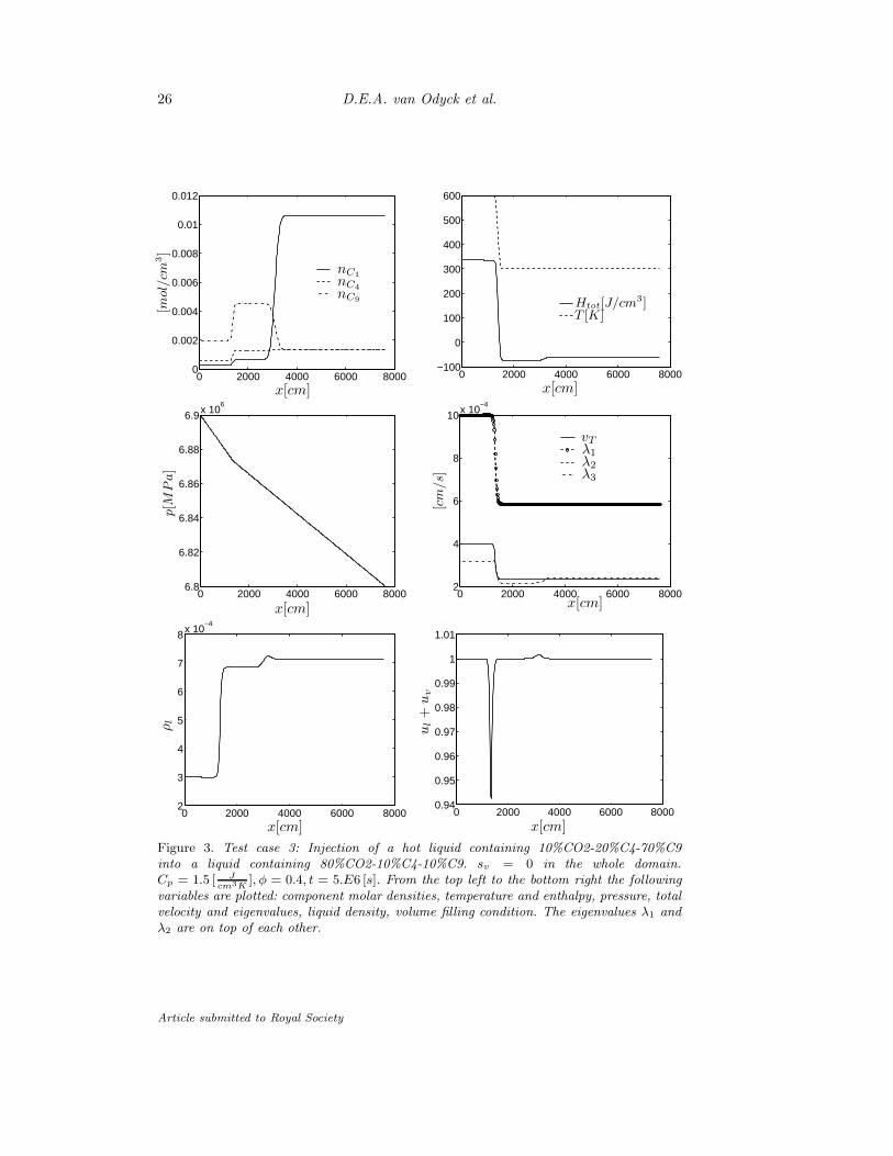
In Test 3 a hot liquid containing 10% methane, 20% butane 70% nonane isinjected into a liquid containing 80% methane, 10% butane, 10% nonane and thedetails of the initial reservoir and boundary conditions are summarised in table 3.The results are plotted in figure 3. This is a single phase liquid simulation. Becauseof the presence of the porous medium there are two distinct wave speeds. Thisresults in a slow wave in the λ3 at around x = 1500 [cm] separated by a constantstate and followed by a faster wave at approximately x = 1500 [cm]. The faster wavecorresponding to λ1, λ2 is essentially a contact discontinuity. Curiously, the slowerwave is also essentially linearly degenerate. The structure in this case is carriedby the change in the total velocity and reflects a change in density resulting fromchanges in compressibility as a function of temperature.

Test 4 is an example of a hot two-phase mixture containing 40% methane, 10%butane, 50% nonane being injected into a colder two-phase mixture containing 80%methane, 10% butane, 10% nonane. The details of the initial reservoir and bound-ary conditions are summarised in table 3. The results, see figure 4, show a rathercomplex behaviour. The hot two-phase mixture first condenses in a small regionahead of the propagating hot front. This is a result of the lagged behaviour of thethermal wave arising because of the heat capacity of the rock. The transition againshows the compound wave behaviour typical of Buckley-Leverett. The mixture thentransitions back into a two-phase mixture with transition between phases accompa-nied by another Buckley-Leverett shock. This multiplicity of waves is made possibleby the loss of strict hyperbolicity shown by the crossing of the eigenvalue curves.



7. Summary and Conclusions

A system of equations describing the flow of non-isothermal multicomponent two-phase fluids in a porous medium has been developed and analysed. The equationsgoverning the system are an extension of the compositional solver developed in(Trangenstein & Bell 1989b). It is shown that the system of equations can be splitinto a hyperbolic system of conservation laws for component density and enthalpyand a parabolic pressure equation that constrains the volume of fluids to the avail-able pore volume. This procedure of decoupling the fundamental equations formsthe basis of a sequential numerical algorithm. The sequential method is then appliedto study four test cases of multi-phase flows that can be encountered in thermalrecovery processes. They demonstrate that the method can resolve the interactingwaves present in the flow field and can shed new light into the understanding ofthe solution structure. The analysis presented here can also form the basis for thedevelopment of higher-order approaches for the component and energy conserva-tion equations and for including additional physical phenomena such as capillarypressure, diffusion and reactions.

DEA van Odyck was funded by Schlumberger Cambridge Research. The work of JohnBell was supported by the Director, Office of Science, of the U.S. Department of Energyunder contract DE-AC02-05CH11231.



References

Acs, G., Doleschall, S. & Farkas, E. 1985 General purpose compositional model. Society

of Petroleum Engineers Journal. 25, 543-552.Bell, J.B., Colella, P. & Trangenstein, J.A. 1989 Higher-order Godunov methods for general

systems of hyperbolic conservation laws. J. Comput. Phys. 82(2) 362-397.Brantferger, K.M. 1991a Development of a thermodynamically consistent, fully im-

plicit,compositional, equation-of-state, steamflood simulator. Ph.D. thesis, The Univer-sity of Texas at Austin, Austin.

Brantferger, K.M., Pope, G.A. & Sepehrnoori, K. 1991b Development of a thermodynam-ically consistent, fully implicit, equation-of-state, compositional steamflood simulator.SPE, 21253, 471-480.

Burger, J., Sourieau, P. & Combarnous, M. 1985 Thermal methods of oil recovery, ch. 1,Editions Technip, Institut Francais du Petrole Publications.

Chen, Z. Huan, G. and Ma, Y. 2006 Computational Methods for Multiphase Flows in

Porous Media, SIAM, Philadelphia.Christensen, J.R., Darche, G., Dechelette, B., Ma, H. & Sammon, P.H. 2004 Applica-

tions of dynamic gridding to thermal simulations. In SPE International Thermal Opera-

tions and Heavy Oil Symposium and Western Regional Meeting, Bakersfield, California,

March 2004.Class, H., Helmig, R. & Bastian, P. 2002 Numerical simulation of non-isothermal multi-

phase multicomponent processes in porous media. Advances in Water Resources, 25,533-550.

Collins, R.E. 1961 Flow of Fluids through Porous Materials, Reinhold Publishing Corp.,New York.

Danesh, A. 1998 PVT and Phase Behaviour of Petroleum Reservoir Fluids, Elsevier, Am-sterdam.

Huang, C.K., Yang, Y.K., & Deo, M.D. 2007 A new thermal-compositional reservoir sim-ulator with a novel “Equation Line-Up” method. In SPE Annual Technical Conference

and Exhibition, Anaheim, California, November 2007.Liu, K., Subramanian, G., Dratler, D.I. & Lebel, J.P. 2007 A general unstructured grid,

eos-based, fully-implicit thermal simulator for complex reservoir processes. In SPE

Reservoir Simulations Symposium, Houston, Texas, 26 February 2007.Mallison, B., Gerritsen, M., Jessen, K. Orr Jr, F.M. 2003 High order upwind schemes for

two-phase, multicomponent flow. In SPE Reservoir Simulation Symposium, Houston,

Texas, February 2003.Michelsen, M.L. 1999 State function based flash specifications. Fluid Phase Equilibria.

158, 617-626.Michelsen, M.L. & Mollerup, J.M. 2004 Thermodynamic Models: Fundamentals & Com-

putational Aspects, Tie-Line Publications, Holte, Denmark.Nilsson, J., Gerritsen, M. & Younis, R. 2005 An adaptive, high-resolution simulation for

steam-injection processes. SPE Western Regional Meeting, Irvine, California, March

2005.O’Connell, J.P. & Haile, J.M. 2005 Thermodynamics, Fundamentals for Applications, pp.

82,88. Cambridge University Press, Cambridge.O’Sullivan, M.J., Pruess, K. & and Lippmann, M.J. 2001 State of the art of geothermal

reservoir simulation. Geothermics, 30, 395-429.Pasarai, U., Arihara, N. & and Waseda, U. 2005 A simulator for predicting thermal recov-

ery behavior based on streamline method. In SPE International Improved Oil Recovery

Conference in Asia Pacific, Kuala Lumpur, Malaysia, December 2005.Peaceman, D.W. 1977 Fundamentals of Numerical Reservoir Simulation, Elsevier.Trangenstein, J.A. & Bell, J.B. 1989a Mathematical structure of black-oil reservoir simu-

lation. SIAM J. Appl. Math., 49, 749-783.Trangenstein, J.A. & Bell, J.B. 1989b Mathematical structure of compositional reservoir

simulation. SIAM J. Sci. Stat. Comput., 10, 817-845.



Appendix A. Partial Derivatives

It is simpler to define the partial derivatives of equation (3.3) at constant T than at con-stant Ht since the equation of state is an explicit function of (T, p,n). Here, we present in

detail the transformation (based on change of variables) to to compute“

∂U∂p

”

n Ht

assuming

that“

∂U∂p

”

n Tis known, by using the fact that:

dU =

„

∂U

∂p

«

nHt

dp +

„

∂U

∂n

«

p Ht

dn +

„

∂U

∂Ht

«

n p

dHt (A 1)

Dividing equation (A1) by dp and taking T constant then gives„

∂U

∂p

«

T

=

„

∂U

∂p

«

n Ht

+

„

∂U

∂n

«

p Ht

„

∂n

∂p

«

T

+

„

∂U

∂Ht

«

n p

„

∂Ht

∂p

«

T

(A 2)

Finally, if one also takes n constant, equation (A2) reduces to„

∂U

∂p

«

n Ht

=

„

∂U

∂p

«

T n

−

„

∂U

∂Ht

«

n p

„

∂Ht

∂p

«

T n

(A 3)

Equation (A3) gives the required transformation to compute“

∂U∂p

”

n Ht

. A similar trans-

formation to compute“

∂U∂Ht

”

n pcan also be obtained by dividing equation (A1) by dT

and taking n and p constant„

∂U

∂T

«

n p

=

„

∂U

∂Ht

«

n p

„

∂Ht

∂T

«

n p

(A 4)

With the help of the above expression, equation (A3) can now be rewritten as a functionof the primitive variables n, p and T and can be calculated explicitly.

„

∂U

∂p

«

n Ht

=

„

∂U

∂p

«

T n

−

„

∂Ht

∂T

«

−1

n p

„

∂Ht

∂p

«

n T

„

∂U

∂T

«

n p

(A 5)

In a similar way one can derive„

∂U

∂n

«

p Ht

=

„

∂U

∂n

«

T p

−

„

∂Ht

∂T

«

−1

n p

„

∂Ht

∂n

«

p T

„

∂U

∂T

«

n p

(A 6)

and„

∂U

∂Ht

«

p n

=

„

∂Ht

∂T

«

−1

n p

„

∂U

∂T

«

n p

(A 7)

In order to compute (A5), (A 6) and (A 7), the partial derivatives of Ht with respectto T , p and n are required. Since Ht is the total enthalpy of the system, the enthalpy ofthe surrounding rock should be taken into account. Therefore Ht can be expressed as:

Ht = (1 − φ)Hs + φHf , Hs = ρrHr , Hf = nTl hl + nT

v hv (A 8)

Assuming that φ = φ(p) and Hs = Hs(T ), then the partial derivatives of Ht with respectto the primitive variables now become:

„

∂Ht

∂T

«

n p

= (1 − φ)

„

∂Hs

∂T

«

n p

+ φ

„

∂Hf

∂T

«

n p

(A 9)

„

∂Ht

∂p

«

n T

= −dφ

dpHs +

dφ

dpHf + φ

„

∂Hf

∂p

«

n T

(A 10)

„

∂Ht

∂n

«

p T

= φ

„

∂Hf

∂n

«

p T

(A 11)



Appendix B. Secant Method

In order to solve equation (5.1) the Secant method is used. In the following the term flash

is used to refer to a phase equilibrium calculation at given (n, p). Given an initial enthalpyH1 and temperature T1 the algorithm looks like:

H1f = 1

φ(H1 − (1 − φ) Crock

p (T1 − T rockref )

flash(H1f ) → T

f1 = H1 − (1 − φ) Crockp (T − T rock

ref ) − φH1f = (1 − φ) Crock

p (T1 − T )T2 = T1 + ∆TH2

f = 1φ(H1 − (1 − φ) Crock

p (T2 − T rockref )

flash(H2f ) → T



p (T2 − T )

T3 = T2 −(T2−T1)(f2−f1)

f2

for l = 1 to Niter doH3

f = 1φ(H1 − (1 − φ) Crock

p (T3 − T rockref ))

flash(H3f ) → T



p (T3 − T )

T4 = T3 −(T3−T2)(f3−f2)

f3

err = ‖T4−T3

T3‖

if err < ǫ thenstop

end ifT2 = T3

f2 = f3

T3 = T4

end for

In the numerical simulations described in Section 6 ∆T = 10. [K] and ǫ = 1 · 10−6.



Table 1. Simulation details for the different test cases.

Test 1 Test 2 Test 3 Test 4

fpress 1. 1. 1. 0.6

∆t 500 ∆x 500 ∆x 1000 ∆x 5∆x

t [s] 1.E8 3.E7 5.E6 5.E5

Table 2. Injection and reservoir condition for Test cases one and two.

Test 1 Test 2

Injection Reservoir Injection Reservoir

nC1[mol/cm3] 0.005385 0.001365 0.005385 0.001365

nC4[mol/cm3] 0.000277 0.001365 0.000277 0.001365

nC9[mol/cm3] 5.6684E-6 0.004096 5.6684E-6 0.004096

φ 1. 1. 0.4 0.4

Crockp [J/cm3/K] 0. 0. 1.5 1.5

P [MPa] 13.80331E6 13.78952E6 13.80331E6 13.78952E6

T [K] 800. 344.3 800. 344.3

H [J/cm3] 56.7385 -127.7710 478.9954 -4.9384

Table 3. Injection and reservoir condition for Test cases three and four.

Test 3 Test 4

Injection Reservoir Injection Reservoir

nCO2[mol/cm3] 0.000284 0.010603 0.000246 0.002109

nC4[mol/cm3] 0.000567 0.001325 0.000616 0.000264

nC9[mol/cm3] 0.001985 0.001325 0.001601 0.000264

φ 0.4 0.4 0.4 0.4

Crockp [J/cm3/K] 1.5 1.5 0.25 0.25

P [MPa] 6.9E6 6.8E6 3.9E6 3.8E6

T [K] 600. 300. 550. 300.

H [J/cm3] 335.8399 -59.1795 75.6951 -6.2640



0 2000 4000 6000 80000

1

2

3

4

x 10−3

x[cm]

[mol

/cm

3]

nC1

nC4

nC9

0 2000 4000 6000 8000−200

0

200

400

600

800

x[cm]

T [K]Htot[J/cm3]

0 2000 4000 6000 80001.3788

1.379

1.3792

1.3794

1.3796

1.3798

1.38

1.3802

1.3804x 107

x[cm]

p[M

Pa]

4500 5000 5500 6000

1

1.5

2

2.5

x 10−4

x[cm]

[cm

/s]

vTλ1λ2λ3

0 2000 4000 6000 80000

0.2

0.4

0.6

0.8

1

x[cm]

s v

0 2000 4000 6000 80000.9993

0.9994

0.9995

0.9996

0.9997

0.9998

0.9999

1

1.0001

x[cm]

ul+

uv

Figure 1. Test case 1: Injection of a hot vapour containing 95%C1-4.9%C4-0.1%C9 into

a liquid containing 20%C1-20%C4-60%C9. Cp = 0. [ J

cm3K], φ = 0.4, t = 1.E8 [s]. From

the top left to the bottom right the following variables are plotted: component molar densi-

ties, temperature and enthalpy, pressure, total velocity and eigenvalues, vapour saturation,

volume filling condition.



0 2000 4000 6000 80000

1

2

3

4

5x 10−3

x[cm]

[mol

/cm

3]

nC1

nC4

nC9

0 2000 4000 6000 8000

0

200

400

600

800

x[cm]

T [K]Htot[J/cm3]

0 2000 4000 6000 80001.3788

1.379

1.3792

1.3794

1.3796

1.3798

1.38

1.3802

1.3804x 107

x[cm]

p[M

Pa]

0 2000 4000 6000 80000

2

4

6

8x 10−4

x[cm]

[cm

/s]

vTλ1λ2λ3

0 2000 4000 6000 80000

0.2

0.4

0.6

0.8

1

x[cm]

s v

0 2000 4000 6000 80000.98

0.985

0.99

0.995

1

1.005

x[cm]

ul+

uv

Figure 2. Test case 2: Injection of a hot vapour containing 95%C1-4.9%C4-0.1%C9

into a liquid reservoir containing a mixture of 20%C1-20%C4-60%C9.

Cp = 1.5 [ J

cm3K], φ = 0.4, t = 3.E7 [s]. From the top left to the bottom right the

following variables are plotted: component molar densities, temperature and enthalpy,

pressure, total velocity and eigenvalues, vapour saturation, volume filling condition.



0 2000 4000 6000 80000

0.002

0.004

0.006

0.008

0.01

0.012

x[cm]

[mol

/cm

3]

nC1

nC4

nC9

0 2000 4000 6000 8000−100

0

100

200

300

400

500

600

x[cm]

T [K]Htot[J/cm3]

0 2000 4000 6000 80006.8

6.82

6.84

6.86

6.88

6.9x 106

x[cm]

p[M

Pa]

0 2000 4000 6000 80002

4

6

8

10x 10−4

x[cm]

[cm

/s]

vTλ1λ2λ3

0 2000 4000 6000 80002

3

4

5

6

7

8x 10−4

x[cm]

ρl

0 2000 4000 6000 80000.94

0.95

0.96

0.97

0.98

0.99

1

1.01

x[cm]

ul+

uv

Figure 3. Test case 3: Injection of a hot liquid containing 10%CO2-20%C4-70%C9

into a liquid containing 80%CO2-10%C4-10%C9. sv = 0 in the whole domain.

Cp = 1.5 [ Jcm3K

], φ = 0.4, t = 5.E6 [s]. From the top left to the bottom right the following

variables are plotted: component molar densities, temperature and enthalpy, pressure, total

velocity and eigenvalues, liquid density, volume filling condition. The eigenvalues λ1 and

λ2 are on top of each other.



0 2000 4000 6000 80000

1

2

3

4x 10−3

x[cm]

[mol

/cm

3]

nC1

nC4

nC9

0 2000 4000 6000 8000−100

0

100

200

300

400

500

600

x[cm]

T [K]Htot[J/cm3]

0 2000 4000 6000 80003.8

3.82

3.84

3.86

3.88

3.9x 106

x[cm]

p[M

Pa]

500 1000 1500 2000 25000

2

4

6

8

10

12

x 10−3

x[cm]

[cm

/s]

vTλ1λ2λ3

0 2000 4000 6000 80000

0.2

0.4

0.6

0.8

1

x[cm]

s v

0 2000 4000 6000 80000.998

1

1.002

1.004

1.006

1.008

x[cm]

ul+

uv

Figure 4. Test case 4: Injection of a hot mixture containing 40%CO2-10%C4-50%C9 into

a mixture containing 80%CO2-10%C4-10%C9. Cp = 0.25 [ J

cm3K], φ = 0.4, t = 5.E5 [s].

From the top left to the bottom right the following variables are plotted: component mo-

lar densities, temperature and enthalpy, pressure, total velocity and eigenvalues, vapour

saturation, volume filling condition.


Documents

The mathematical structure of multiphase thermal · PDF fileThe mathematical structure of multiphase thermal models of ... for modelling multicomponent, two-phase, thermal ﬂuid ﬂow