Thermal simulation in multiphase incompressible … Lagrangian particle level set method with second-order reinitialization is introduced, for the first time in thermal simulations,

Available online at www.sciencedirect.com

ScienceDirect

Comput. Methods Appl. Mech. Engrg. 336 (2018) 667–694www.elsevier.com/locate/cma

Thermal simulation in multiphase incompressible flows usingcoupled meshfree and particle level set methods

M. Afrasiabia,b,∗, M. Roethlinb, K. Wegenerb

a Institute of Structural Engineering (IBK), D-BAUG, ETH Zürich, Stefano-Franscini-Platz 5, 8093 Zürich, Switzerlandb Institute of Machine Tools & Manufacturing (IWF), D-MAVT, ETH Zürich, Leonhardstrasse 21, 8092 Zürich, Switzerland

Received 15 January 2018; received in revised form 12 March 2018; accepted 13 March 2018Available online 27 March 2018

Abstract

A particle-based numerical solver is presented, applicable to the simulation of heat transfer in multiphase immiscible flowsincluding surface tension. In the context of meshfree methods, the Laplacian operator is recognized as the most numericallychallenging ingredient of the heat equation. The well-known difficulty of approximating higher-order spatial derivatives withmeshfree methods is herein addressed by adopting two advanced schemes in order to ensure second-order accuracy. In addition,a Lagrangian particle level set method with second-order reinitialization is introduced, for the first time in thermal simulations, tocapture the location of the interface, i.e., moving and/or deformable boundaries of the continuum at each time-step. This leadsto a more conservative solution, alleviating the mass loss during the simulation. Furthermore, a narrow band of the exteriorgeometric particles is exploited to form physical ghost particles to enforce the required boundary conditions. This novel approachensures solver performance without the necessity of defining extra dummy particles for treating boundary conditions in meshfreesimulations. Three benchmark problems are considered for evaluating the performance of the proposed solver against a referenceanalysis performed in COMSOL Multiphysics R⃝.c⃝ 2018 Elsevier B.V. All rights reserved.

Keywords: Meshfree methods; Multiphase flows; Heat transfer; Moving interfaces; Particle level set

1. Introduction

Ever since its inception in the late 70s [1,2], Smoothed Particle Hydrodynamics (SPH) has been applied to adiverse spectrum of applications, including, but not limited to, solid [3–5] and fluid [6–8] mechanics problems,even though the initial exploitation primarily pertained to astrophysics and gas dynamic problems. Thanks to thetremendous growth of computing power, there has been a renewed interest in applying SPH to sophisticated fields,beyond engineering applications, such as virtual reality surgery, movies special effects and computer graphics [9–11].Interestingly enough, alternative particle models to simulate fracture and damage in solids have also been attemptedin various works, as elaborated upon in [12–14].

∗ Correspondence to: ETH Zurich, Institute of Machine Tools & Manufacturing (IWF), Technoparkstrasse 1, 8005 Zurich, Switzerland.E-mail address: [email protected] (M. Afrasiabi).

https://doi.org/10.1016/j.cma.2018.03.0210045-7825/ c⃝ 2018 Elsevier B.V. All rights reserved.

http://crossmark.crossref.org/dialog/?doi=10.1016/j.cma.2018.03.021&domain=pdf

http://www.elsevier.com/locate/cma

https://doi.org/10.1016/j.cma.2018.03.021

http://www.elsevier.com/locate/cma

mailto:[email protected]

https://doi.org/10.1016/j.cma.2018.03.021

668 M. Afrasiabi et al. / Comput. Methods Appl. Mech. Engrg. 336 (2018) 667–694

SPH methods have been extensively and successfully adopted by the Computational Fluid Dynamics (CFD)community as evidenced by the numerous applications [6,15–21]. The weakly compressible SPH (WCSPH) models,as the original formulation of SPH for fluid dynamics, comprise one of the most efficient strategies for solvingincompressible fluid dynamics problems. Using WCSPH, the admissible density fluctuations of the fluid is boundedand kept relatively small, hence treating the fluid as quasi-incompressible. This may be achieved by employing aproper equation of state, which links density to hydrodynamic pressure. The interfacial flows simulation by Colagrossiand Landrini [22], the multiphase SPH investigations of macroscopic and mesoscopic flows by Hu and Adams [23],and the extensive SPH analysis of bubble evolution in up to 3D problems by Zhang et al. [24] are some of thesuccessful attempts reported in the state of the art, to name a very few.

Meshfree methods in problems involving heat conduction, although applicable, are not as well-established asthe family of the Finite Element (FE) methods. This stems from the fact that the meshfree approximation of theLaplacian of temperature in heat conduction PDEs is nontrivial. A Lagrangian discretization of the heat equation,nonetheless, is required when designing a meshfree solver for problems wherein thermal issues cannot be neglected.This has led to a remarkable body of research, which already exists concerning the improvement of contemporarymeshfree methods from both the complexity and accuracy points of view. In 1995, a Reproducing Kernel ParticleMethod (RKPM) [25,26] was introduced, which is capable of improving the accuracy of higher-order derivativesby satisfying the target moment condition. Later, a Corrective Smoothed Particle Method (CSPM) was formulatedby Chen et al. [27] for unsteady heat conduction problems in 2D. Eldredge et al. [28] showed that the frameworkused to develop Particle Strength Exchange, often termed as PSE, can be generalized to approximate arbitrary spatialdifferential operators. In 2011, a novel meshfree scheme was developed for approximating the Laplacian operator byFatehi and Manzari [29]. This work was nominated for the latest “Monaghan Prize”. They incorporated an innovativerenormalization tensor to amend the inaccuracy of higher derivatives, especially in the vicinity of the boundaryparticles. Most recently, an improved CSPM (ICSPM) scheme has been derived and used for 2D heat conductionproblems with fixed-in-space particles [30]. When approximating the Laplacian operator, numerical experiments showthat the accuracy of Fatehi’s results is comparable with ICSPM, whereas the computational overhead in the former isconsiderably higher. As a result, two second-order accurate schemes are employed for the desired applications in thiswork: PSE and ICSPM, to be discussed more comprehensively in Section 3. Some state-of-the-art meshfree workswould additionally contain a broad array of applications from 2D heat equation with non-classical boundary conditionsand diffusion-wave equation in [31,32] to generalized telegraph and diffusion equations published by [33,34], forinstance.

The computational representation of the interface comprises a dedicated mechanism of its own, forms an activearea of current research. Since CFD simulations involve the generation of new surfaces as guided by fluid flows, theassociated geometric evolution influences not only the accuracy of the solution but also the reliability of the physicalfield variables. The need to capture complex topological features is therefore dictates the choice of method to modelmoving interfaces in CFD problems. In addition to Lagrangian [35–37] and Eulerian [38,39] methods, which havebeen adopted in the computational solution of moving interfaces, the so-called class of hybrid Particle Level Set (PLS)approaches has further been developed for such problems.

The first hybrid PLS method, in the spirit of Enright et al. [40], improves the level set (LS) values at Eulerian gridsby means of Lagrangian marker particles. The Lagrangian PLS method introduced by Hieber and Koumoutsakos [41],overcomes the difficulties associated with the Lagrangian formulation of level set (LS) equations, via adoption oftechniques extensively discussed in [42], and further developed for vortex particle methods in [43,44]. Akin to theoriginal SPH idea [1,2], kernel functions are adopted to mollify the LS functions, which are subsequently discretizedusing particles as quadrature points. In order to ensure accuracy a remeshing procedure was first introduced withinthe context of LS methods in [41]. This method was then extended in the work of Bergdorf and Koumoutsakos [45],where a multiresolution Lagrangian particle method with enhanced, wavelet-based adaptivity is presented for transportproblems, fusing the efficiency of wavelet collocation with the inherent numerical stability of particle methods. Inrecent work, Cottet et al. [46] offer a treatise on the definition and implementation of remeshed particle methodswithout LS reinitialization, offering a consistency and stability analysis of a large class of second- and fourth-ordermethods. The elegance of PLS methods lies in the coexistence of particles and grids, coupling the accuracy ofLagrangian advection with the simplicity of the Eulerian level set surface representation. The PLS technique proposedby Hieber and Koumoutsakos [41], hereinafter EPLS, is herein enhanced for use in the problem of thermal simulations.To the best of the authors’ knowledge, there is no work in literature dedicated to the incorporation of PLS method into

M. Afrasiabi et al. / Comput. Methods Appl. Mech. Engrg. 336 (2018) 667–694 669

meshfree thermal models. A primary objective of this paper lies in proposing a truly second-order PLS for interfacecapturing in thermal simulations. Attention must be paid while considering a geometry representation problem due tothe common fallacy of tracking (explicit) vs. capturing (implicit) terminology.

In the present work, a selective SPH formulation for multiphase immiscible flows is introduced wherein thesurface tension effect is also taken into account. The functionality of this formulation is verified by several numericalexamples where internal flow, bursting at free surface, bubble evolutionary split–merge motions, and coalescenceoccur. The modeling of heat transfer in the aforementioned SPH formulation is currently lacking literature. Herein,two second-order meshfree methods, namely PSE and ICSPM, are employed for simulating heat transfer in problemsof multiphase flows motivated by the compromise of accuracy vs. computational cost. The Lagrangian PLS methodin [41] is enhanced with a second-order reinitialization scheme implemented for the first time in thermal simulations,and is utilized to more accurately capture the location of the interface at each time-step. For analyzing the thermalissues in multiphase flows where the interface is exposed to complex topological evolutions (e.g. coalescence, bursting,separation, reformation, and so on), three segments shall work altogether. First, a versatile multiphase flow simulatoris executed in order to calculate the velocity field in multiphase flows. Second, an efficient meshfree solver forheat conduction is presented, which is second-order accurate. Third, a precise Lagrangian method for capturingmoving interfaces is introduced by enhancing the conventional PLS to a second-order reinitialized PLS (EPLS).Consequently, this paper offers a coupling of these three backbones in a versatile meshfree tool for simulating complexthermal problems. The method is demonstrated on examples which illustrate its potential for thermal simulation inmultiphase incompressible flows. Albeit not theoretically or numerically validated herein, the enhanced PLS methodused bears the potential of second-order accuracy, and offers results that are superior to a reference commercialsoftware implementation.

This manuscript is organized as follows: a generic meshfree formulation for modeling multiphase immiscible flowsis briefly reviewed in Section 2. Next, in Section 3 the two selected methods (i.e., PSE and ICSPM) are separatelyreviewed, through which the heat equation will be discretized. Discussed in Section 4 is a relatively comprehensiveoutline of the proposed EPLS technique for handling the problems of moving interfaces. The corresponding numericaltest cases follow in Section 5. Lastly, the article concludes in Section 6 with a discussion on the performance of theinnovative coupling of the proposed meshfree methods in CFD simulations. The concluding remarks are followed bythe outlook towards future research.

2. Meshfree formulation of multiphase flows

The improvement of meshfree formulations to solve the complex problems of multiphase flows is still a verydynamic field of research according to the numerous alternatives for multiphase SPH models that may be found incurrent literature [6,7,23,24,47–50]. Since the meshfree formulation of multiphase flows itself is a very challengingtopic, and the major focus of this work is not on investigation of such formulations, only a summary of the selectedscheme for handling the applications at hand is herein projected.

In a Lagrangian framework, the governing equations for the motion of an isothermal fluid consist of the continuityand momentum equations. A suitable equation of state has yet to be taken into consideration while simulatingincompressible fluids with the WCSPH approach. In the following, the aforementioned equations are approximatedvia the selective meshfree approach to deliver a versatile numerical solver for the problem at hand.

2.1. Mass conservation

By definition, the material derivative in a velocity field of v is given as

DDt

=∂

∂t+ v · ∇ (1)

and the mass conservation, i.e., continuity, equation at point i will consequently read

Dρi

Dt= −ρi∇ · vi (2)


where ρi is the density of point i . For the sake of consistency, the following notation is applied throughout this paper⎧⎪⎪⎨⎪⎪⎩♦ if ♦ is a zeroth-order tensor (scalar)♦ if ♦ is a first-order tensor (vector)♦ if ♦ is a second-order tensor♦≈

if ♦ is a fourth-order tensor

(3)

The continuity equation, Eq. (2), can be discretized for particle i using SPH formulations, as also used byMonaghan [51]⟨dρi

dt

⟩= ρi

N∑j=1

V j(vi j · ∇Wi j

)(4)

if the smoothing kernel Wi j (r i j , h) is abbreviated to Wi j wherein h denotes the smoothing length, and r i j is the relativedistance vector between particle i and j . The gradient of Wi j is ∇Wi j , and the relative velocity between particle i andj is vi j = vi − v j . Also, the volume contribution of particle j is represented by V j =

m jρ j

in which m j denotes themass of particle j . It was shown in [52] that the “quintic spline” function or the “renormalized Gaussian” function arethe most efficient kernels among 10 alternatives in terms of computational cost vs. accuracy. These two kernels arethus adopted for the numerical simulations in this work. Note that ⟨♦⟩ denotes a numerically approximated value of♦ in this paper.

Though the upper bound of the summation in Eq. (4), N , is the total number of the particles in the domain, thecut-off radius of the smoothing kernel truncates the neighboring search into a smaller sub-domain, hence performingthe summation only on the neighbors of particle i rather than all N particles. It is worth repeating that the currentdiscretization in Eq. (4) of the continuity equation is chosen for the applications in this work due to its ability tohandle multiphase problems without any further manipulation/adjustment.

To approximate the density of each particle, the smoothed density formulation introduced in [2] and furthersuggested by Hu and Adams [23] is employed. This is particularly beneficial when considering the models in whichthe large density ratios at multiphase interfaces exist. Such is the case, for instance, of a gaseous bubble travelingthrough a heavier liquid and reaching the surface (i.e., ρliq ≫ ρgas). The density of particle i with the mass mi is thencalculated from a summation over its all neighboring particles j

⟨ρi ⟩ =mi

⟨Vi ⟩= mi

N∑j=1

Wi j (5)

Through this smoothing sum, Eq. (5) allows for density discontinuities and, like almost all other SPH methods,conserves the total mass exactly.

2.2. Conservation of momentum

Consistent with Newton’s second law of motion, the transport of momentum is governed by the incompressibleNavier–Stokes equations including the surface tension. This equation can be written symbolically where theLagrangian discretization point i , say particle i , is driven by four different volumetric forces expressed in the right-hand side of the following equation

ρiDvi

Dt= −∇ pi

Fpri

+ µi∇2vi

Fvii

+ f sti

Fsti

+ ρi gFb f

i

(6)

coupled with the incompressibility constraint as

∇ · vi = 0 (7)

In Eq. (6), µi is the dynamic (shear) viscosity of particle i and g represents the gravitational acceleration.From now on, the superscripts “pr”, “vi”, “st”, and “b f ” indicate the pressure, viscous, surface tension, andbody force contributions, respectively. The numerical approximations of the above mentioned terms are discussedindividually.


2.2.1. Pressure termTo start with, the driven force (per unit volume) of particle i due to a pressure gradient, as outlined in [24], can be

approximated as

⟨F pri ⟩ = −

1Vi

N∑j=1

(pi V 2

i + p j V 2j

)∇Wi j (8)

The present formulation for pressure gradient is energy conservative thanks to the principle of virtual work, whichhas been applied to the derivation of this expression in the corresponding work by Zhang et al. [24]. This can bereplaced with the pressure term, F pr

i , in Eq. (6).

2.2.2. Viscous termNext, the viscous term Fvi

i at particle i needs to be evaluated. To this end, the following form, which is well-suitedfor multiphase flows, is taken according to [23,53,54]

⟨Fvii ⟩ = ηd

N∑j=1

V jµi jvi j · r i j

|r i j |2+ (ϵh)2

∇Wi j (9)

with µi j =2µi µ jµi +µ j

designating the combined dynamic viscosity, and ηd = 2(nd + 2) if nd represents the spatialdimensions, which is equal to 2 in our test cases. To guard against the zero denominator in Eq. (9) where two particlesget too close to each other, a reasonably small parameter ϵ = 0.01 is used as well. Employing the present discretizationof the viscous term in Eq. (9), both linear and angular momenta are conserved, according to [24].

2.2.3. Surface tension termWhen modeling multiphase problems, the surface tension is formed at the interfacial layer due to the variation

of Van der Wall’s force in different fluid phases. This should not be ignored, neither can it be underestimated,in designing a robust numerical tool; especially if the deformation and the topology of the fluid interface are ofparamount influence for the specified problem. Among several alternatives in literature, the model devised by Adamiand Adams [49] is henceforth used for treating the surface tension effect. This scheme is physically more meaningfulthan the conventional model by Morris [55], but is also able to reflect the real asymmetric surface tension forceincorporating a density-weighted color gradient to approximate the curvature of the interface between two differentphases. More interestingly, Adami’s model was shown in [24] to be the most accurate approach amongst availablesurface tension schemes in SPH, especially in treating the problems where the density ratio of interacting phasesis significantly large. It was proven that by reproducing divergence approximation the accuracy of the curvaturecalculation can remarkably be improved.

Here, the two principal geometric entities to be calculated are the unit normal vector and the curvature at thelocation of the interface. In accordance with [49], these two values for particle i are respectively calculated via

ni =ni

|ni |=

∇ci

|∇ci |(10)

κi = −∇ · ni∼= −nd

∑Nj=1 V j

(ni − λ

ji n j

)· ∇Wi j∑N

j=1 V j |r i j ||∇Wi j |(11)

It is important to note that the above mentioned formulation works due to the zeroth-order completeness of SPH.This matter has been thoroughly discussed in [56]. In Eqs. (10) and (11), λ

ji is the corrector switch to invert the

direction of the unit normal

λji =

−1 if particle i and j belong to different phases+1 if particle i and j belong to the same phase (12)

and the gradient of ci in Eq. (10) can be defined numerically as [49]

∇ci =1Vi

N∑j=1

(V 2

i + V 2j

) cii + c j

i

2∇Wi j (13)


in which the index number c ji based on Adami’s scheme is a density-weighted color function and can be formulated

as

c ji =

⎧⎪⎪⎨⎪⎪⎩2ρi

ρi + ρ jif particle i and j belong to different phases

0 if particle i and j belong to the same phase

(14)

As demonstrated in [49] the recent manipulation for defining the weight function in Eq. (14) delivers a continuousdistribution of the acceleration across the interfacial particles. Having calculated the magnitude of the curvature at thetarget particle i , one can determine the corresponding contribution of its surface tension into the momentum equation,and substitute F st

i in Eq. (6) with its numerical approximation as suggested by [49]

⟨F sti ⟩ = −σκi |∇ci |ni (15)

which relates the surface tension coefficient σ to the geometric entities at the interfacial particles.

2.2.4. Body force termFinally, the term Fb f

i in Eq. (6) is simply replaced with the corresponding gravitational acceleration in therespective spatial directions for particle i as long as there is no external force exerted to the body

Fb fi = ρi g (16)

By doing so, all components in Eq. (6) are eventually known for all particles in a given time-step.

2.3. Equation of state

Assuming a barotropic fluid plus applying an equation of state, the mass and momentum conservation equationscan be uncoupled [6]. In other words, an appropriate equation of state is indeed necessary for evaluating the pressureof each particle with regards to the corresponding density field. This is a numerical surrogate for the incompressibilitycondition (∇ · v = 0) in Navier–Stokes equations, which is a nontrivial task for meshfree methods to enforceanalytically. This stringent constraint is usually satisfied by means of numerical approximation. A proper and well-established choice for this purpose is Tait’s equation of state, as reported in several related works [6,7].

pi = p0

[(ρ

ρ0

)γ

i− 1

]+ χ (17)

In Eq. (17), it is recommended to use γ = 1.4 and γ = 7 for gases and fluids, respectively [6]. Also, the incidenceof negative pressures, i.e., tensile instability mode, is hampered by utilizing a positive background pressure χ . In orderfor the pressure field to be equal to χ initially, the reference density ρ0 is set to the initial density of the fluid phase.Our numerical experiments suggest that a value between 2% − 10% of the initial pressure is satisfactory for a stablesimulation in most applications. Unless otherwise mentioned, χ = 0.05 p0 is used in this work by default. Accordingto [6,7], the numerical value of the reference pressure is also expressed as

p0 =c2ρ0

γ(18)

where c stands for the artificial sound speed in the given fluid. Morris et al. [7] showed that by performing a scaleanalysis c can be estimated in a way that the threshold of the admissible density variation is limited to 1%, hencefulfilling the weakly-compressible criterion.

2.4. Wall boundary condition

To enforce the boundary conditions in multiphase SPH models, the generalized wall approach, first introduced byAdami et al. [57], is employed in the present work. In their approach, “ghost particles” are used. Put briefly, the “ghostparticles” are virtual points inheriting the physical properties of their corresponding actual particle. The solid wallsare initially filled with these dummy particles to retrieve the incomplete support domain of the smoothing kernel,


which is cut by the domain boundaries. Contrary to the so-called “mirror particles” approach [7], this generalized“ghost particles” scheme does not require any explicit geometric information of the boundaries. As described in theoriginal work [57], these physical properties of the ghost particles are determined accordingly to impose the no-slipconditions: velocity, pressure, and density

vg = 2vpsg −

∑a va Wga∑

a Wga(19)

pg =

∑a pa Wga + (g − aps

g ) ·∑

a ρar ga Wga∑a Wga

(20)

ρg = ρ0,a

[(pg − χ

p0,a

)+ 1

] 1γ

(21)

where the subscripts “g” and “a” are designating the “ghost” and “actual” particles. The superscript “ps” refers to theprescribed values of the wall velocity and acceleration. Note that none of these values are evolved in time, meaningthey do not participate in the time integration procedure.

2.5. Time integration

A second-order velocity-Verlet scheme is adopted for updating the equation of motion and the momentum equationin time [58]. This scheme is summarized for particle i at the nth step as follows

vn+

12

i = vni +

∆t2

(dvi

dt

)n

(22)

rn+

12

i = rni +

∆t2

vn+

12

i (23)

ρn+1i = ρn

i + ∆t(

dρi

dt

)n+12

(24)

rn+1i = r

n+12

i +∆t2

vn+

12

i (25)

vn+1i = v

n+12

i +∆t2

(dvi

dt

)n+1

(26)

In Eqs. (22) to (26), the step size of this integration, ∆t , is calculated such that it meets the following criterionglobally.

∆t = 0.5 × min(∆tvi ,∆tcs,∆tb f ,∆tst

)(27)

wherein the CFL-conditions [6,24,50,51] for the viscous, artificial sound speed, body force, and surface tension, arerespectively computed from⎧⎪⎪⎪⎪⎪⎪⎪⎪⎪⎪⎪⎪⎪⎪⎪⎪⎪⎨⎪⎪⎪⎪⎪⎪⎪⎪⎪⎪⎪⎪⎪⎪⎪⎪⎪⎩

∆tvi = C F Lviρ(∆x)2

ν, C F Lvi = 0.125

∆tcs = C F Lcs∆x

(cmax + |v|max ), C F Lcs = 0.25

∆tb f = C F Lb f

√∆x|g|

, C F Lb f = 0.25

∆tst = C F Lst

√ρ(∆x)3

2πσ, C F Lst = 0.25

(28)

if ∆x is the initial particle spacing.


3. Meshfree discretization of heat equation

The general governing PDE for transient heat transfer is expressed as

ρcp∂T∂t

= ∇(k∇T ) + Qin − Qv (29)

in which cp is specific heat capacity, T temperature, k heat conductivity, Qin the heat source and Qv heat loss per timeand volume. The surface heat source, Qin , originates from the internal flows and will be described in the respectiveexamples in Section 5. Qv is herein assumed to be zero, meaning no heat is lost upon radiation, nor via convection.

As mentioned earlier in Section 1, PSE and ICSPM will be exploited for approximating the heat conductionequation in the proposed model. These two strong-form meshfree methods are revisited in the following. On a separatenote, it is worthwhile to point out the possibility of reducing the order of the differential operators, i.e., herein secondderivatives, in view of weak-form meshfree formulations, variational principle, and partial integration. This strategywould require a background grid, and is not of the present paper’s interest, however.

To ensure the overall stability of the numerical solution in this section, the time-step size associated with theheat equation in Eq. (29) needs to be limited to a critical value as well. Akin to what was mentioned in Eq. (27), aCFL-condition is often assumed based on the minimum distance discretization distance, and a global minimum valuemust be chosen together with the time-step size criteria outlined in Eq. (28). This matter is automatically met in thesimulations presented since the time-step size linked to the CFD part in this investigation is always smaller than theone from the stability analysis of the heat equation (supposing a Courant number of 0.25 for a given particle ensemblein the thermal part).

3.1. Particle strength exchange

Originally introduced for treating the Laplacian term in advection–diffusion problems [59–61], Particle StrengthExchange method, is known as a strong numerical tool for solving diffusion problems. As a well-established fieldof application, PSE has been extensively used in a diverse application range of vortex methods [28,62]. In brief, onecan derive a second-order PSE kernel between particles i and j for two-dimensional Laplacian operator, as expressedin [28]

W PSEi j (r i j , h) =

4πh2 exp(−|q|

2) (30)

where q =|r |

h . As described in [28], using this kernel together with a numerical quadrature for integral approximation,a second-order approximation of the Laplacian of the temperature T at particle i can thus be obtained as follows⟨

∆Ti

⟩PSE=

1h2

N∑j=1

V j (T j − Ti )W PSEi j (31)

This formulation can consequently be used for approximating the heat conduction equation for the application athand.

3.2. Improved CSPM

Inspired by the same idea behind the CSPM approach [27], Korzilius et al. showed that a second-order accurateapproximation of the second derivatives can be obtained by the incorporation of the first derivative approximationwhich is one order higher accurate [30]. One may digress briefly to remind that the numerical approximation of firstderivatives is prerequisite for approximating the second derivatives with CSPM. As elaborated upon in [27], the CSPMapproximations for the first and second derivatives of T are calculated from⎧⎪⎪⎪⎨⎪⎪⎪⎩

⟨∂T∂x

⟩

⟨∂T∂y

⟩

⎫⎪⎪⎪⎬⎪⎪⎪⎭i

:=

⟨∇Ti

⟩CSPM= A−1

i

[ N∑j=1

V j (T j − Ti )∇Wi j

](32)


⎡⎢⎢⎢⎢⎣⟨

∂2T∂x∂x

⟩ ⟨∂2T∂x∂y

⟩

⟨∂2T∂y∂x

⟩ ⟨∂2T∂y∂y

⟩

⎤⎥⎥⎥⎥⎦i

:=

⟨∇∇Ti

⟩CSPM

= B≈

−1i

[ N∑j=1

V j (T j − Ti )∇∇Wi j −

N∑j=1

V j

(r j i ·

⟨∇T

⟩CSPM

i

)∇∇Wi j

]

RHS

(33)

where ⊗ denotes the tensor product. The CSPM renormalization tensors Ai

and B≈ i

for the first and second derivativesat the target particle i are defined as

Ai=

N∑j=1

V j(r j i ⊗ ∇Wi j

)(34)

B≈ i

=

N∑j=1

V j

(C

i j⊗ ∇∇Wi j

)(35)

in which for 2D problems

Ci j

=

⎡⎢⎢⎢⎣12

(xi − x j )(xi − x j ) (xi − x j )(yi − y j )

(yi − y j )(xi − x j )12

(yi − y j )(yi − y j )

⎤⎥⎥⎥⎦ (36)

If one higher-order term in the corresponding Taylor series of ∇ f in Eq. (32) is included as well, the improvedapproximation for the first derivatives can be calculated as first derived in [30]⟨

∇Ti

⟩ICSPM=

⟨∇Ti

⟩CSPM− A−1

i

[ N∑j=1

12

V j

(r j i

[∇∇T

]ir j i

)∇Wi j

](37)

By taking[∇∇Ti

]out of the summation, and simplifying by a mathematical factorization, the ICSPM representa-

tion for the second derivatives arrives at the following form by taking into account the same RHS defined in Eq. (33)⟨∇∇Ti

⟩ICSPM= D

≈

−1i

[RHS

](38)

wherein the new renormalization tensor D≈

is computed from

D≈ i

= B≈ i

−

[⎛⎝ N∑j=1

V j (r j i ⊗ ∇∇Wi j )

⎞⎠ · Ai·

⎛⎝ N∑j=1

V j (C i j⊗ ∇Wi j )

⎞⎠](39)

This extra renormalization matrix needs to be computed for each particle i when and whenever the particlelocation is changed (i.e., deformation/distortion of the body). The final form of the second-order approximation ofthe Laplacian of the temperature T at particle i using ICSPM is the sum of the elements on the main diagonal, i.e., the

trace, of⟨∇∇Ti

⟩ICSPMin Eq. (38)⟨

∆Ti

⟩ICSPM= tr

[⟨∇∇Ti

⟩ICSPM]

(40)

The temperature T in Eqs. (31) and (40) can be substituted by any other field function of interest. It is alsoworth noting that the recently described scheme is able to reconstruct the second derivatives with higher accuracyin comparison with CSPM, while its extra computational effort is, strictly speaking, negligible.


4. Computational moving interfaces

As noted in Section 1, the representation of the interface is a key piece of the proposed numerical toolkit. BothEulerian and Lagrangian perspectives are concisely reviewed in the following. This section closes by introducing theproposed EPLS approach for the interface capturing of distorted flows.

4.1. Eulerian representation of level set methods

On one hand, the Eulerian viewpoint is to embed a fixed mesh of grid points, and represent the interface “implicitly”as a level contour of a function. This type of method is called “interface capturing”. The family of the Level Set (LS)methods is the most well-known approach for capturing propagating interfaces originally introduced by Osher andSethian in 1988 [38]. At its core, the LS technique hinges on viscosity solutions for Hamilton–Jacobi equations.This shares the virtues of working in an arbitrary number of space dimensions with no change and handles topologicalmerger and splitting with no special procedures. LS method can efficiently compute the motion of fronts moving undercomplex speed laws, including large variations in velocities and sharp discontinuities. A multitude of workaroundshas been however employed to recover the violation of “mass conservation”, recognized as the major drawback of theLS method, among which, the two hybrid approaches cited in Section 1 have seen a broader exploitation.

The fundamental idea behind the LS method is merely to define a smooth scalar function ϕ(x, t), that representsthe interface as the isocontour where ϕ(x, t) = 0 (zero level set is actually the interface). Note that the position vectoris x = (x1, x2, x3, . . . , xn) in general, if n determines the number of the spatial dimensions. Now, given an interfaceΓ (t) in Rn of codimension one, bounding an open region Ω , the subsequent motion of Γ (t) under a velocity fieldv is desired. This velocity may or may not depend on position, time, the geometry of the interface (e.g., its normalor its mean curvature), and the external physics. By definition, the LS function ϕ maintains the following built-incharacteristics⎧⎨⎩ϕ(x, t) < 0 if x ∈ Ω

ϕ(x, t) = 0 if x ∈ Γ (t)ϕ(x, t) > 0 if x ∈ Ω

(41)

Clearly, the motion of the interface Γ (t) is embedded in the motion of the LS function ϕ(x, t), and can be analyzedthrough the advection equation. This is accomplished mathematically by convecting the ϕ values (i.e., levels) with thegiven velocity field v, which in an Eulerian framework is expressed as

∂ϕ

∂t+ v · ∇ϕ = 0 (42)

One can notice that Eq. (42) is attributed to Initial Value Problems (IVPs) often known as the standard Hamilton–Jacobi equation, hence requires to know the initial values of ϕ as

ϕ(x, 0) = ϕ0(x) (43)

There are numerous choices to pick for ϕ0(x), among which the Signed Distance Function (SDF) sees a broaderrange of applications. Given a set Ω in a metric space with the boundary (i.e., interface) of Γ , the SDF of each pointp is defined as the distance of p from Γ , with the sign determined by whether p is in Ω . The convention is to assignthe negative sign to the SDF values at points p inside Ω . The SDF decreases in value as p approaches the boundaryof Ω where the SDF is zero, and it takes positive values outside of Ω . Unless noted, SDF is chosen for ϕ0(x) in thispaper.

4.2. Lagrangian representation of level set methods

On the other hand, for Lagrangian methods, points are placed directly on the interface and move with the interface.For example, in a 2D case, this can be visualized by nodes (buoys) along the curve which are connected by linesegments (ropes). Sometimes for stability purposes, points on the interface are permitted to move in the tangentialdirection, too. For this type of method, the interface location is “explicitly” known. This type of method is called“interface tracking”. Adopting the “interface tracking” approach, however, one may suffer from an inability to modelchanges in topology (pinching and merging) of the interface [63–66]. Although purely Lagrangian particles are more


accurately moved through space, they alone are not capable of representing a dynamic surface such as water jet,bubble merging, and fire. The problem is that when the simulation is updated, the distribution of particles can becomevery uneven, resulting in unresolved areas where there are not enough particles to properly represent a surface (oroverly condensed/accumulated). The second problem inherent in a particle only method is that a surface still needs tobe defined and doing so based on particles is not a straightforward task.

Contrary to the Eulerian representation of LS method in which the LS information is convected through thestationary grids, the LS characteristics in a Lagrangian representation are carried by non-stationary particles. Thus,Eq. (42) can be reformulated in a Lagrangian description for particle p as

Dϕp

Dt= 0

Dx p

Dt= v p (44)

where x p indicates the characteristics of the equation for this particle.

4.3. Particle level set method

Upon a comprehensive study of several benchmarks in the state of the art, it turns out that a versatile computationalapproach for representing the complex geometries is barely found on solely Eulerian or solely Lagrangian frameworks.Hybrid PLS methods may instead be adopted, as mentioned in the introductory section and as elaborated upon in[41,46,67,68]. In these methods, grids and particles always go hand in hand for treating the complicated problems ofmoving interfaces. In essence, the PLS description of interest is built on the Lagrangian representation of LS methodsas discussed in Section 4.2. Succinctly, the method initiates with the configuration of particles and then performs aconsistent remeshing procedure onto uniformly-spaced particles to regularize the particle locations when the particlemap gets distorted by the advection field. In the following, the principal formulation of PLS is explained.

Evolution of a body in the Lagrangian framework is comprehended by solving a system of Ordinary DifferentialEquations (ODEs) on the representative particles, derived from the principal equation Eq. (42)

Dϕp

Dt= 0

Dx p

Dt= v p

DVp

Dt= Vp

(∇ · v p

)(45)

in which x p is the position vector of particle p, Vp is the particle volume, and ϕp is its level set value. It is worthmentioning that the proposed PLS is supposed to bear the intrinsic property of returning null error in all rigid bodymotions. Nonetheless, the numerical errors induced by both particle initialization and the numerical time integrationmay still exist. In order to acquire a fully second-order PLS for a precise representation of the geometry, the followingset of conditions should be met:

• a second/higher-order accurate particle approximation for field variables and their spatial derivatives• a second/higher-order accurate time integration scheme for advecting particles• a second/higher-order accurate interpolation kernel for the remeshing procedure• a second/higher-order accurate reinitialization technique

The aforementioned conditions are scrutinized separately in a consecutive manner. It is worth clarifying that theterm “second-order accurate” is related to the order of convergence with the increase of N , while the “second-ordercompleteness” pertains to the reconstruction of second-order polynomials with the null error.

4.3.1. Particle approximationsOnce the particles are initialized, their level set values are calculated for the problem at hand. According to Eq. (45),

ϕp is kept unchanged on particles during the evolution. As already discussed in Section 3, two alternative second-ordermeshfree schemes can be utilized for constructing the first two derivatives in this paper. The particle approximationis required for the computation of the geometrical entities such as the unit normal and the curvature of the interface.


Fig. 1. Illustration of the remeshing procedure: (a) scattered particles are given, (b) a superimposed regular mesh is generated, (c) the interpolationkernel on each particle is performed, (d) affected regular grids are found, (e) the affected regular grids become new particles, (f) non-affected meshgrids are deleted. This figure follows the same structure presented in work [69] of Koumoutsakos et al.

The unit normal n and the curvature κ , as already formulated in Eqs. (10) and (11), are redefined for non-physicalparticle p

n p =∇ϕp

|ϕp|(46)

κp = ∇ ·∇ϕp

|ϕp|(47)

wherein the gradient and Laplacian operators can be replaced with the previously mentioned particle approximationsin Section 3.

4.3.2. Particle advectionGiven the velocity field, particles are advected using a discretized time integration scheme. A fourth-order Runge–

Kutta (RK4) method is selected to evolve the non-physical particles in all simulations of the present work. This choice,in turn, guarantees the satisfaction of the second condition needed for the proposed PLS, listed in Section 4.3. Bothparticle positions and volumes are thus updated in accordance with the second and the third equations (45), while theirdistance to the interface remains constant within the evolution.

4.3.3. RemeshingThe underpinning of having a robust tool for capturing the interface by the present PLS relies on the remeshing

procedure, further elaborated upon in [41,46,67–69]. From left to right, this procedure is schematically representedstep by step in Fig. 1. In accordance with the first utilization of remeshing in PLS methods [41], a brief descriptionof this procedure is herein revisited. Although remeshing can directly be applied to physical particles and havesuccessfully been used in some related works (e.g., [67,70]), this approach may however cause some difficultiesin handling wall boundary conditions which would require additional considerations. This matter is thus not takeninto account for the present work.

Frequent remeshing is performed in the course of PLS simulations in order to retain the “particle overlapcondition”, but also to obtain a smooth well-defined representation of the interface. The “particle overlap condition”is referred to as a term by which the distance between the particles should always be smaller than their core size. Sincethe severely scattered locations of the particles are quite likely to happen in problems undergoing involute velocityfields, the incorporation of the remeshing procedure seems inevitable to regularize the distorted particle arrangements.With these goals in mind, two interpolation kernels employed in this work are given. By definition, θn,m(s) is a kernelthat interpolates the characteristic s by preserving the moment conservation up to the order n, and creates a smoothinterpolated function which is mathematically Cm continuous. Often termed as M ′

4, the commonly-used interpolationkernel is given by [41]

θ2,1(s) =

⎧⎪⎪⎪⎨⎪⎪⎪⎩1 −

12

(5s2− 3s3)2 if 0 ⩽ s < 1

12

(2 − s)2(1 − s) if 1 ⩽ s ⩽ 2

0 if 2 < s

(48)


For the numerical simulations of this work, a higher-order kernel is employed, according to [46,71]

θ4,4(s) =

⎧⎪⎪⎪⎪⎪⎪⎪⎪⎪⎪⎪⎪⎪⎪⎪⎪⎪⎪⎪⎪⎪⎪⎪⎪⎨⎪⎪⎪⎪⎪⎪⎪⎪⎪⎪⎪⎪⎪⎪⎪⎪⎪⎪⎪⎪⎪⎪⎪⎪⎩

1 −54

s2+

14

s4−

1003

s5+

4554

s6−

2952

s7 if 0 ⩽ s < 1

+345

4s8

−115

6s9

−199 +5485

4s1

−32975

8s2

+28425

4s3

−61953

8s4 if 1 ⩽ s < 2

+33175

6s5

−20685

8s6

+3055

4s7

−1035

8s8

+11512

s9

5913 −89235

4s1

+297585

8s2

−143895

4s3

+177871

8s4 if 2 ⩽ s ⩽ 3

−54641

6s5

+19775

8s6

−1715

4s7

+345

8s8

−2312

s9

0 if 3 < s

(49)

It is noteworthy that the interpolation kernel in a multi-dimensional domain, Θn,m , is the Cartesian tensorialmultiplicative of its 1D counterparts θn,m . For 2D problems, it reads

Θn,m(s1, s2) = θn,m(s1)θn,m(s2) (50)

in which the characteristics of s1 and s2 are determined by s1 =|x p2m |

δx and s2 =|yp2m |

δy . Note that |ξp2m | is the 1Ddistance of the scattered particle from the uniform background particle, i.e., mesh, in ξ−direction, and δξ is thespacing of the uniform particles in ξ−direction.

Due to the limited-range communication of particle p with the background grid nodes in its vicinity, the time effortfor interpolating particle property to mesh is of O (N ), with N is the total number of particles. Depending on thecomplexity of the geometry and the applied velocity field, the frequency of the remeshing procedure may vary fromcase to case. The criterion to define this frequency often stems from a measure of distortion (c.f. [41]) or any user-defined parameter ascribed to the irregularity of the particle distribution. Unless otherwise mentioned, the remeshingis performed only when this criterion exceeds a certain prescribed threshold. As offered by Hieber et al. in [41], therate at which the remeshing procedure has to be called is usually based on the fact that at time t the weighted sumH(t) over all N particles must be equal to unity in a regularized particle map. For particle i , this propounds

Hi (t) =

N∑j=1

V j Wi j (51)

H(t = 0) = H(0) = 1 (52)

A suitable measure of distortion is consequently defined by averaging the change of H(t) over all particles as

∆H(t) =1N

N∑j=1

|H j (t) − H j (0)|H j (0)

(53)

In theory, ∆H(t) should be zero for all rigid body motions. Nevertheless, and because the numerical tests of thepresent work are not fallen into the rigid body motions, this distortion threshold is set to a prespecified value equalto 10−6 in the simulations conducted. Care has yet to be taken regarding the computation of the corrector matrix ofparticle i expressed in Eq. (39), whether the same measure of distortion can be similarly used. Albeit it would be infavor of the computational effort, the distortion criterion discussed in Eq. (53) is only used for geometric purposes inthis work, and the ICSPM corrector matrix is indifferently recomputed for each particle at each time-step.

4.3.4. ReinitializationAssuming SDF as the initial values for ϕ, it generally does not preserve its property after evolving under a general

velocity field. In other words, the LS function can quickly cease to be SDF, especially for flows undergoing extremetopological changes. However, one can reinitialize the ϕ values by finding (a new) ϕ with:


Fig. 2. Schematic higher-order multistencils for IFMM. Color coded is the order of neighboring nodes: 1st-order nodes in black, 2nd-order nodesin blue, and redundant 2nd-order nodes in yellow. (For interpretation of the references to color in this figure legend, the reader is referred to theweb version of this article.)

• the same zero level set (meaning the interface)• and |∇ϕ| = 1

The former condition asserts that reinitialization procedure should not, but may, change the location of the interface,hence is no anti-erosion treatment for the level set evolutions. The latter assures a smooth variation of ϕ, meaning itdoes not become too flat or too steep near the interface. Some widely-used reinitialization techniques are distancereinitialization using a smooth signum function [72], the Fast Marching Method (FMM) [73–75], and the FastSweeping Method (FSM) [76].

The reinitialization method used in this work is an improved Higher Accuracy Fast Marching Method (HAFMM)which was introduced in [77], as further adopted in the work of Hieber and Koumoutsakos [41]. Two types ofenhancements are here applied to the current HAFMM to enable a second-order accurate reinitialization method.The improved FMM proposed in this manuscript is termed as IFMM, for the sake of brevity. Firstly, the ignoredinformation provided by diagonal neighboring particles in Cartesian coordinates are retrieved by incorporating themultistencils framework as suggested by Hassouna et al. [78]. Illustrated in Fig. 2 is the schematic depiction ofthe multistencils used in IFMM wherein the target node, as well as its axial and diagonal first neighboring nodes,are shown in black. Secondly, a bicubic interpolation scheme is adopted for initializing the fast marching method.This is achieved by constructing a second-order approximation of the interface generated from local data on theparticles. Initially published by Chopp [79], it was shown in his work that this improvement allows for a second-order approximation of the distance to the interface, which can then be used to produce second-order accurate initialconditions for FMM.

Since the reinitialization methods such as FMM and FSM are implementable only on regularly-spaced compu-tational elements, dispersed particle locations hamper these methods to execute. It is thus necessary to ascertainthe regularity of the computational elements for reinitialization purposes. This requirement is automatically met inthe proposed PLS method thanks to the exploitation of the remeshing algorithm discussed in Section 4.3.3, if thefrequency of remeshing is equal or higher than the frequency of the reinitialization procedure.

5. Simulation results

In this section, the performance of the methods presented, namely the WCSPH scheme coupled with thePSE/ICSPM and EPLS, in applications to two-dimensional problems is investigated. It should be noted that thepresented examples aim in demonstrating the potential of the method in coupled thermal flow simulations. Theenhanced PLS method used bears the potential of second-order accuracy, based on fulfillment of the conditionsoutlined in section 4.3. However, we leave the theoretical and numerical validation of second-order accuracy forseparate discussion in future work. Towards this end, the following three test cases are considered

• Model 1: vortex flow as a deforming internal heat source (prescribed velocity field)• Model 2: heat transfer in single rising oil bubble (non-prescribed velocity field)• Model 3: synthetic heat conduction in two coalescing bubbles (non-prescribed velocity field)

For each model, two different sets of particles, namely “physical” and “geometrical”, are introduced initially. Whilethe properties discussed in Sections 2 and 3 are carried by “physical” particles, “geometrical” particles are responsible


Table 1Summary of the parameters in “model 1”.

Property Dimension Value

Density kg m−3 1Specific heat capacity J kg−1 K−1 470Heat conductivity W m−1 K−1 20Initial temperature K 293.15Heat source per unit volume W 108

Width of container m 1.0Height of container m 1.0Initial radius of circle m 0.15Initial position of circle m (0.5, 0.75)

to resolve the respective characteristics of the moving interfaces, elaborated in Section 4. An equal particle spacing isassumed in the initial configurations of both particle types for all simulations.

5.1. Vortex flow as a deforming heat source

A synthetic benchmark is designed in order to accentuate the crucial role of a robust tool for capturing the locationof the interface at each time-step, where the multiphase meshfree model plays no role. The same classical single vortexgeometry is studied according to [40]. The importance of this example is embedded in the significance of an accurateinterface representation for imposing the associated boundary conditions in bodies undergoing extreme deformations,but also to evaluate the robustness of the proposed solver in solving thermal equations. Suppose the heat is only addedto the interior domain, i.e., the white areas in Fig. 3. As can be seen in Fig. 3, the geometry of the heat source at eachstep encounters a severe deformation, which necessitates a precise definition of the interface. The numerical values ofthe parameters used in this simulation are listed in Table 1, as follows.

The multiphase flow solver is not invoked in this case because the velocity field is constant and given as

v =π

314

⎧⎨⎩0.5 − y

x − 0.5

⎫⎬⎭ [ms

](54)

First off, the given interface is driven by the above mentioned velocity field in Eq. (54) without incorporating anythermal effect. This geometric evolution of the white body can be followed in the consecutive snapshots of Fig. 3.

In order to demonstrate the improvement gained by the proposed EPLS method, the vortex interface is extractedat t = 3, as shown in Fig. 4. A regular 256 × 256 particles resolution is used as the initial setup, incorporating theIFMM reinitialization scheme. The EPLS approach markedly improves the resolution of the captured interface, butalso decrease the mass loss in comparison with the reference data obtained from COMSOL Multiphysics R⃝. Thisimprovement leads to a more conservative solution regarding the mass loss deficiency. Moreover, the very smoothand high-quality representation of the interface is observed in Fig. 3, the attribute which was not achievable withLagrangian particles only. It should be noted that the discretization points in both meshfree and FE platforms aredeliberately kept similar for better comparisons. In Fig. 4(c), the LS solution is shown in red, the original PLSsolution [40] in blue, and a high-resolution front-tracked solution in green for the same vortex flow at t = 3.The quality and accuracy of the EPLS representation is comparable to the high-resolution front-tracked solutionin Fig. 4(c).

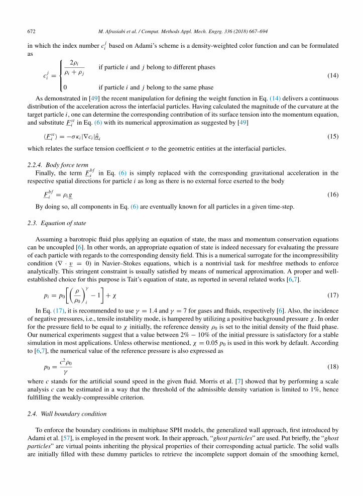
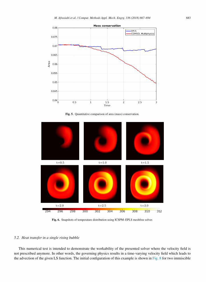
The mass conservation of the proposed EPLS is consequently compared against the COMSOL results in Fig. 5,by which the weaker performance of the COMSOL simulation is understood through its less mass conservative trend,shown in red. Due to the incompressibility of the fluid, the conservation of the area of the white body is shown asrepresentative of its mass.

Once the geometry aspects are handled precisely, the thermal issue is added to the current model. The ICSPMscheme is herein utilized for discretizing the heat conduction equation. As stated in Table 1, the initial temperatureof all particles is set to 293.15 considering the thermal insulation in all wall boundaries. Shown in Fig. 6 are thesnapshots of temperature distribution in time using the coupled ICSPM–EPLS scheme. The obtained results are ingood agreement with the FE solution from COMSOL Multiphysics R⃝ in Fig. 7.


Fig. 3. Representation of the interface in a single vortex with EPLS method.

Fig. 4. Vortex interface at t = 3.

In this example, a periodic remeshing is performed each 20 steps. Besides, the 4th-order kernel θ4,4 expressed inEq. (49) is used for both particle-to-mesh and mesh-to– particle interpolations.

As illustrated in Fig. 5 and discussed earlier, the mass loss in the proposed solution is notably less compared to theone in COMSOL. This more conservative solution accordingly introduces more heat charge, especially for later steps,hence the higher maximum temperature in the final step. It is also worth highlighting that the area inside the vortexfor the EPLS method is computed approximately by multiplying the number of interior particles and the allocatedcorresponding area for each particle. For a more accurate estimation, a multiplier of α = 0.5 for all interfacialparticles with −

∆2 < ϕ < 0 is used, where ∆ is the initial particle spacing. This multiplier would be α = 1.0 for

all other interior particles. The numerical errors from the calculation of the confined area and also the smoothingeffects due to the remeshing procedure can explain the existing inaccuracy in the mass conservation of this approach.Meanwhile, four periodic overshoots are noticed along the EPLS temporal mass conservation in Fig. 5. The reasonfor this behavior lies in the periodic reinitialization procedure. In fact, the IFMM algorithm is called each 20 steps,while the whole simulation is performed in overall 90 steps.


Fig. 5. Quantitative comparison of area (mass) conservation.

Fig. 6. Snapshots of temperature distribution using ICSPM–EPLS meshfree solver.

5.2. Heat transfer in a single rising bubble

This numerical test is intended to demonstrate the workability of the presented solver where the velocity field isnot prescribed anymore. In other words, the governing physics results in a time-varying velocity field which leads tothe advection of the given LS function. The initial configuration of this example is shown in Fig. 8 for two immiscible


Fig. 7. Snapshots of temperature distribution using COMSOL MultiphysicsR⃝.



Oil density kg m−3 879Water density kg m−3 1000Oil viscosity Pa s 0.0208Water viscosity Pa s 0.00101Surface tension coefficient N/m 0.015Oil specific heat capacity J kg−1 K−1 1970Water specific heat capacity J kg−1 K−1 4185Oil heat conductivity W m−1 K−1 0.150Water heat conductivity W m−1 K−1 0.585Oil initial temperature K 343Water initial temperature K 293Wall initial temperature K 318

Width of container m 0.010Height of container m 0.015Initial position of bubble m (0.0, 0.004)Initial diameter of bubble m 0.004

fluids, in which four different regions exist: the initially immersed oil bubble (blue label), the stagnant oil at the topof the container (blue label), the surrounding water (yellow label), and the solid walls (red label). Listed in Table 2 isalso the summary of all parameters used in the simulation for this buoyancy-driven oil bubble.

Since the velocity field is no longer known a priori in “model 2” and “model 3”, the velocity of the physicalparticles are interpolated into the locations of the geometrical particles. The quintic spline kernel is used for thispurpose. Furthermore, and unlike “model 1”, the measure of distortion is applied as the commencement condition ofremeshing procedure for the following two models.

As can be understood from the label plot in Fig. 8, the wall boundaries are represented with three layers of ghostparticles to ensure the completeness of the supporting domain for the chosen smoothing kernel (i.e., the quintic spline


Fig. 8. Initial configuration of “model 2”. (For interpretation of the references to color in this figure legend, the reader is referred to the web versionof this article.)

Fig. 9. Variation of the maximum density error (left) and evolution of the y-component of the bubble’s center of mass (right).

kernel with cut-off radius of 3h). A fairly low resolution of 41 × 61 particles is considered to emphasize the robustnessof the proposed solver even without using fine discretization. As expected, the oil bubble travels upwards through thewater phase and merges with the oil layer already residing at the top of the container. The moving fluid–fluid interfacedue to the buoyancy effect is captured by invoking the velocity field computed from the Navier–Stokes equations.

Vividly, buoyancy effects cause the immersed oil bubble to rise within the water phase. As the bubble touches theupper liquid–liquid interface, it merges with the oil phase, starts to oscillate shortly, reaches to the stability and standsstill finally. This scenario is clearly observed through the consecutive snapshots in Fig. 10. When solving a model withreal physical properties, it is important to assume a physically meaningful surface tension coefficient in order to attaina stable numerical simulation. The topology of the bubble is substantially affected by the value of this coefficient. Theparameter used in this case is hence assumed to be the oil–water surface tension at room temperature, as included inTable 2.

To ensure the credibility of the WCSPH formulation, the variation of the density error is also calculated over time.Through this evaluation, as demonstrated in Fig. 9, one can notice that the maximum variation in density is reasonablyless than the acceptable limit of 1% − 5%. It must be emphasized again that the initial background pressure in this


Fig. 10. Interface evolution using EPLS (top) and COMSOL MultiphysicsR⃝ (bottom).

meshfree formulation plays the pivotal role in controlling the density variation upon the equation of state, i.e., Eq. (17),hence avoiding the occurrence of the so-called “tensile instability”. Furthermore, the y−component of the bubble’scentroid is tracked as a measure of the bubble evolution in time, plotted in Fig. 9.

The EPLS result shows a good qualitative agreement with the corresponding output from COMSOL, as shown inFig. 10. The finite element based LS solution in COMSOL is obtained by setting the CFD modules as predefined physicsinterfaces, augmented by the “Laminar Two-Phase Flow” as well as the “Level Set” interfaces. One of the salientfeatures of the proposed meshfree toolkit is that it delivers acceptable accuracy even with such a low resolution,which is an appealing characteristic from the computational cost point of view.

Fig. 11 permits several perceptions. Firstly, a better conservation of mass in EPLS solver is observed comparedto the reference data. Secondly, the EPLS solution is indifferent to the two critical moments of t ≃ 0.20 andt ≃ 0.26, whereas the mass conservation in COMSOL is greatly influenced. These moments are associated with whenthe uprising oil bubble first hits with the stagnant oil layer above and creates several transient waves before reachingthe steady state. To address the thermal effect in this example, the PSE scheme is coupled with the EPLS method. Theinfinitesimal mass gain in EPLS at t ≃ 0.2 that can be noticed in Fig. 11, although may seem counter-intuitive at thefirst glance, comes from the remeshing with regards to the impulsive distortion at that time. This is exactly the timewhen the bubble bursts at the oil surface. Regulating the reinitialization frequency as well as the measure of distortionwould modify this behavior for the problem at hand.

The temperature distribution using PSE–EPLS solver alongside the solution of COMSOL are depicted in Fig. 12for the five corresponding time instants. This comparison conveys a good agreement between the PSE–EPLS andFE results. For a better visualization and a clearer comparison with the FE outputs, all the snapshots in Fig. 10 andFig. 12 display only the half of the domain due to the existing symmetry condition in the present model. However, themeshfree simulations presented were carried out on the whole domain, while the COMSOL simulations were performedon the half-domain imposing the axial symmetry condition.


Fig. 11. Quantitative comparison of mass conservation.

Fig. 12. Comparison of temperature distributions.

5.3. Heat conduction in coalescing bubbles

The last benchmark is concerned with a multiphase flow in which several scenarios are to be tackled. This examplestudies the coalescence of two co-axial bubbles followed by the bursting at the lighter fluid interface. The results of theproposed solver are validated by the numerical data through a finite element based LS method carried out in [80]. Theinitial setup of the present test is depicted in Fig. 13 along with the description of the physical parameters representedin Table 3. The domain is discretized by 81 × 161 uniformly-spaced particles plus three layers of ghost particles forimposing the no-slip wall boundary conditions.

The physical scenarios of “model 2” and “model 3” are not entirely dissimilar. In fact, a co-axial coalescence ofthe two bubbles is anticipated prior to hitting the interface. Because of the capillary instability, the thin fluid film issplit into a transient and then gradually deforms into a circular liquid droplet under the surface tension effect. Later




Phase-A density kg m−3 100Phase-B density kg m−3 1000Phase-A viscosity Pa s 99Phase-B viscosity Pa s 49.5Surface tension coefficient N/m 0.072Phase-A specific heat capacity J kg−1 K−1 4185Phase-A heat conductivity W m−1 K−1 50000Phase-A initial temperature K 293.15Phase-B initial temperature K 423.15

Width of container m 3.0Height of container m 6.0Initial position of leading bubble m (0.0, 1.0)Initial position of trailing bubble m (0.0, 2.0)Initial diameter of leading bubble m 1.0Initial diameter of trailing bubble m 0.8

Fig. 13. Initial configuration of “model 3”.

on, this newly formed droplet will return to the heavier phase due to the gravitational effect. The whole procedure canbe followed by the consecutive time frames illustrated in Fig. 14. The use of Lagrangian LS approach appears moreadvantageous than the classical Eulerian LS method in modeling the fluid film rupture and droplet formation, whereinmore detailed physical phenomena can be seized by the EPLS approach.

Qualitative comparison of the snapshots in Figs. 14 and 15 shares several key observations. Although being adeptin the modeling of interfacial flows, the Eulerian LS approach seems incompetent versus the proposed Lagrangian LS,especially for interface rupture, reconnection, and very small scale topological evolutions. Investigating the results ofmeshfree (see Fig. 14) and FE-based LS methods (see Fig. 15), one may realize that as soon as the fluid film becomes


Fig. 14. Snapshots of interface evolution using EPLS.

thinner, the two numerical results show some discrepancies. Especially from t = 3.62 to t = 5.5 of the FE-based LSresults in Fig. 15, the fluid film is completely lost in the simulation, which may be ca used by the diffusive nature of theLS method on the Eulerian grids (non-conservative). Using EPLS, nevertheless, the mass is carried by each physicalparticle, hence providing an intrinsic conservation of the mass during the simulation. Furthermore, the insufficientcomputational element number in the LS simulation leads to the inability of capturing the flow details by the coarsediscretization [80].

Finally, the thermal simulation is added to the current benchmark to assess the performance of the proposedmeshfree approximator for discretizing the heat equation. The PSE scheme is utilized for this purpose due to itssimplicity in handling the perfect isolation boundary conditions. The perfect isolation boundary condition is imposedon the four wall boundaries, meaning the initial temperature of the ghost boundary particles is set to be equal to thetemperature of their corresponding physical phase. One shall notice that the heat in this test is solved on the heavierphase only, to better visualize the coupling of the thermal-coalescence process (see Fig. 16). This explains why theheat-related properties were not defined for “Fluid B” in Table 3.

6. Conclusion

A novel coupling of three particle-based solvers existing in the state of the art is proposed: multiphaseincompressible flows with SPH, advanced meshfree thermal solvers, and hybrid Particle Level Set (PLS) methodsfor moving interfaces. The most recent successful attempts from the respective literature are merged in themeshfree solver suggested for multiphase incompressible flows. This includes a multiphase representation ofboth pressure gradient and viscous terms in Navier–Stokes equations together with a robust treatment of surfacetension effect. Regarding the heat conduction problems, two schemes are adopted from the state of the art forapproximating higher order derivatives with meshfree methods. One of these two methods, namely ICSPM, is


Fig. 15. Snapshots of interface and velocity field evolution using FE-based LS [80].

employed to the moving particles application for the first time. In the meantime, an enhanced PLS methodis adopted by incorporating a higher-order reinitialization technique, as well as a more accurate interpolationkernel.

The workability of the present solver is first evaluated in a preliminary synthetic benchmark, demonstrating itsstrength for modeling of thermal aspects subjected to severe deformations (“model 1”) and intricate topologicalchanges (“model 2”, “model 3”). Towards this end, a classical single vortex is supposed to be a highly deformingheat source. The comparative analysis against available data from FE results of COMSOL Multiphysics R⃝ illustratesa remarkable improvement in mass conservation using the meshfree-EPLS solver. This is particularly appealing whenthe linkage of the heat source is directly related to the location of the interface.

Next, two numerical tests are performed where the velocity fields ought to be evaluated from CFD solutions. Thesecase studies pertain to situations in which several physical incidents, such split–merge and bursting of bubbles atthe free surface, need to be displayed. Not only are the interface representations markedly improved by utilizing theEPLS method, but also physical phenomena like mass and heat transfer are more conservatively captured thanksto the Lagrangian nature of the proposed scheme. As shown in Section 5, the employed method is capable ofsimulating thermal phenomena in CFD problems by coupling the WCSPH methodology and the EPLS approach.Another interesting advantage of this novel meshfree-EPLS coupling is that the exterior “geometrical” particles areused as “physical” ghost particles to enforce the boundary conditions.


Fig. 16. Snapshots of temperature distribution using PSE–EPLS.

As a result of this research, subsequent works can be envisioned along diverse directions. An immediate follow-upstudy could deal with a comprehensive performance analysis on the direct replacement of the Laplacian of velocityin the viscous term with contemporary meshfree approximators for higher-order derivatives. It would also be fruitfulto pursue further research about the bilateral privilege of “physical–geometrical” coupling in order to derive a newsurface tension scheme. The more precise representation of the geometrical features, for example, the normal vectorand curvature, can increase the accuracy and/or efficiency of the surface tension force on interfacial particles. Inaddition, a salient step that remains lies in the numerical verification of this scheme as a second-order accurate schemeby means of a thorough convergence study.


The extension of the proposed solver to 3D problems is, theoretically speaking, straightforward. To that end, futurework might as well encompass the parallel and distributed computing implementations on both CPUs and GPUs, inorder to attenuate the very expensive cost of the computations in three-dimensional applications. Consideration ofa “narrow-band” approach is yet another tactic that can craft a more effective solution to the problems of movinginterfaces, by which the computational complexity of the EPLS algorithm could be significantly reduced. By doingso, one would only investigate the geometrical attributes only on the narrow bands around the interfaces rather thanon the full domain. The proposed numerical solver could also be extended to simulations involving ill-defined wallboundaries where the prescribed velocity and acceleration at ghost particles are no longer zero. The functionality ofthis meshfree coupling may eventually be adopted to simulate even more complicated phenomena in manufacturingfields, such as the modeling of laser dry/wet machining and drilling processes. This, in turn, opens up a multitude ofnew avenues to the utilization of robust meshfree solvers into the scope of real-world mechanical and manufacturingproblems.

Acknowledgments

This work was financially sponsored by the Swiss National Science Foundation under Grant No. 200021-149436,which is gratefully acknowledged. The first author would also like to sincerely show his gratitude to Dr. Sven Friedelfor all his lucrative discussions within the course of the COMSOL simulations, as well as Prof. Eleni Chatzi for theinsightful comments and valuable discussion.

References

[1] R.A. Gingold, J.J. Monaghan, Smoothed particle hydrodynamics: theory and application to non-spherical stars, Mon. Not. R. Astron. Soc.181 (3) (1977) 375–389.

[2] L.B. Lucy, A numerical approach to the testing of the fission hypothesis, Astron. J. 82 (1977) 1013–1024.[3] J. Gray, J. Monaghan, Numerical modelling of stress fields and fracture around magma chambers, J. Volcanol. Geotherm. Res. 135 (3) (2004)

259–283.[4] T. Rabczuk, T. Belytschko, Adaptivity for structured meshfree particle methods in 2D and 3D, Internat. J. Numer. Methods Engrg. 63 (11)

(2005) 1559–1582.[5] T. Rabczuk, T. Belytschko, A three-dimensional large deformation meshfree method for arbitrary evolving cracks, Comput. Methods Appl.

Mech. Engrg. 196 (29) (2007) 2777–2799.[6] J.J. Monaghan, Simulating free surface flows with SPH, J. Comput. Phys. 110 (2) (1994) 399–406.[7] J.P. Morris, P.J. Fox, Y. Zhu, Modeling low reynolds number incompressible flows using sph, J. Comput. Phys. 136 (1) (1997) 214–226.[8] M. Afrasiabi, S. Mohammadi, Analysis of bubble pulsations of underwater explosions by the smoothed particle hydrodynamics method, in:

ECCOMAS International Conference on Particle Based Methods, Spain, 2009.[9] M. Müller, S. Schirm, M. Teschner, Interactive blood simulation for virtual surgery based on smoothed particle hydrodynamics, Technol.

Health Care 12 (1) (2004) 25–31.[10] M. Müller, S. Schirm, M. Teschner, B. Heidelberger, M. Gross, Interaction of fluids with deformable solids, Comput. Animat. Virtual Worlds

15 (3–4) (2004) 159–171.[11] A. Nealen, M. Müller, R. Keiser, E. Boxerman, M. Carlson, Physically based deformable models in computer graphics, in: Computer Graphics

Forum, vol. 25, Wiley Online Library, 2006, pp. 809–836.[12] E. Schlangen, E. Garboczi, Fracture simulations of concrete using lattice models: computational aspects, Eng. Fract. Mech. 57 (2–3) (1997)

319–332.[13] R. Rezakhani, G. Cusatis, Asymptotic expansion homogenization of discrete fine-scale models with rotational degrees of freedom for the

simulation of quasi-brittle materials, J. Mech. Phys. Solids 88 (2016) 320–345.[14] R. Rezakhani, X. Zhou, G. Cusatis, Adaptive multiscale homogenization of the lattice discrete particle model for the analysis of damage and

fracture in concrete, Int. J. Solids Struct. 125 (2017) 50–67.[15] A.K. Chaniotis, D. Poulikakos, P. Koumoutsakos, Remeshed smoothed particle hydrodynamics for the simulation of viscous and heat

conducting flows, J. Comput. Phys. 182 (1) (2002) 67–90. http://dx.doi.org/10.1006/jcph.2002.7152.[16] M.B. Liu, G.R. Liu, K.Y. Lam, Adaptive smoothed particle hydrodynamics for high strain hydrodynamics with material strength, Shock

Waves 1 (15) (2006) 21–29. http://dx.doi.org/10.1007/s00193-005-0002-1. Retrieved February 1, 2017.[17] Nicolas Grenier, et al., An Hamiltonian interface SPH formulation for multi-fluid and free surface flows, J. Comput. Phys. 228 (22) (2009)

8380–8393.[18] Mingyu Zhang, Xiao-Long Deng, A sharp interface method for SPH, J. Comput. Phys. 302 (2015) 469–484.[19] S.J. Lind, P.K. Stansby, Benedict D. Rogers, Incompressible–compressible flows with a transient discontinuous interface using smoothed

particle hydrodynamics (SPH), J. Comput. Phys. 309 (2016) 129–147.[20] F.R. Ming, P.N. Sun, A.M. Zhang, Numerical investigation of rising bubbles bursting at a free surface through a multiphase SPH model,

Meccanica 52 (11–12) (2017) 2665–2684.

http://refhub.elsevier.com/S0045-7825(18)30146-4/sb1

































http://dx.doi.org/10.1006/jcph.2002.7152

http://dx.doi.org/10.1007/s00193-005-0002-1












[21] A. Obeidat, S.P.A. Bordas, Three-dimensional remeshed smoothed particle hydrodynamics for the simulation of isotropic turbulence, Int. J.Numer. Methods Fluid 86 (2018) 1–19. http://dx.doi.org/10.1002/fld.4405.

[22] A. Colagrossi, M. Landrini, Numerical simulation of interfacial flows by smoothed particle hydrodynamics, J. Comput. Phys. 191 (2) (2003)448–475.

[23] X. Hu, N.A. Adams, A multi-phase SPH method for macroscopic and mesoscopic flows, J. Comput. Phys. 213 (2) (2006) 844–861.[24] A. Zhang, P. Sun, F. Ming, An SPH modeling of bubble rising and coalescing in three dimensions, Comput. Methods Appl. Mech. Engrg. 294

(2015) 189–209.[25] W.K. Liu, S. Jun, Y.F. Zhang, Reproducing kernel particle methods, Internat. J. Numer. Methods Fluids 20 (8–9) (1995) 1081–1106.[26] S. Jun, W.K. Liu, T. Belytschko, Explicit reproducing kernel particle methods for large deformation problems, Internat. J. Numer. Methods

Engrg. 41 (1) (1998) 137–166.[27] J. Chen, J. Beraun, T. Carney, A corrective smoothed particle method for boundary value problems in heat conduction, Internat. J. Numer.

Methods Engrg. 46 (2) (1999) 231–252.[28] J.D. Eldredge, A. Leonard, T. Colonius, A general deterministic treatment of derivatives in particle methods, J. Comput. Phys. 180 (2) (2002)

686–709.[29] R. Fatehi, M. Manzari, Error estimation in smoothed particle hydrodynamics and a new scheme for second derivatives, Comput. Math. Appl.

61 (2) (2011) 482–498.[30] S. Korzilius, W. Schilders, M. Anthonissen, An Improved CSPM approach for accurate second-derivative approximations with SPH, J. Appl.

Math. Phys. 5 (01) (2016) 168.[31] E. Shivanian, More accurate results for two-dimensional heat equation with neumann’s and non-classical boundary conditions, Eng. Comput.

32 (4) (2016) 729–743.[32] V.R. Hosseini, E. Shivanian, W. Chen, Local radial point interpolation (MLRPI) method for solving time fractional diffusion-wave equation

with damping, J. Comput. Phys. 312 (2016) 307–332.[33] E. Shivanian, A. Khodayari, Meshless local radial point interpolation (MLRPI) for generalized telegraph and heat diffusion equation with

non-local boundary conditions, J. Theoret. Appl. Mech. 55 (2) (2017) 571–582.[34] E. Shivanian, A. Jafarabadi, Rayleigh–Stokes problem for a heated generalized second grade fluid with fractional derivatives: a stable scheme

based on spectral meshless radial point interpolation, Eng. Comput. 34 (1) (2018) 77–90.[35] M.S. Longuet-Higgins, E. Cokelet, The deformation of steep surface waves on water. i. a numerical method of computation, Proc. R. Soc.

Lond. Ser. A Math. Phys. Eng. Sci. 350 (1660) (1976) 1–26.[36] G.R. Baker, D.I. Meiron, S.A. Orszag, Generalized vortex methods for free-surface flow problems, J. Fluid Mech. 123 (1982) 477–501.[37] S.T. Grilli, P. Guyenne, F. Dias, A fully non-linear model for three-dimensional overturning waves over an arbitrary bottom, Internat. J. Numer.

Methods Fluids 35 (7) (2001) 829–867.[38] S. Osher, J.A. Sethian, Fronts propagating with curvature-dependent speed: algorithms based on Hamilton-Jacobi formulations, J. Comput.

Phys. 79 (1) (1988) 12–49.[39] S. Osher, R. Fedkiw, Level Set Methods and Dynamic Implicit Surfaces, vol. 153, Springer Science & Business Media, 2006.[40] D. Enright, R. Fedkiw, J. Ferziger, I. Mitchell, A hybrid particle level set method for improved interface capturing, J. Comput. Phys. 183 (1)

(2002) 83–116.[41] S.E. Hieber, P. Koumoutsakos, A lagrangian particle level set method, J. Comput. Phys. 210 (1) (2005) 342–367.[42] Roger W. Hockney, James W. Eastwood, Computer Simulation Using Particles, crc Press, 1988.[43] G.-H. Cottet, P. Koumoutsakos, Vortex Methods – Theory and Practice, Cambridge University Press, New York, 2000.[44] P. Koumoutsakos, A. Leonard, High-resolution simulation of the flow around an impulsively started cylinder using vortex methods, J. Fluid

Mech.[45] M. Bergdorf, P. Koumoutsakos, A Lagrangian particle-wavelet method, Multiscale Modeling Simul. 5 (3) (2006) 980–995.[46] G.-H. Cottet, et al., High order semi-Lagrangian particle methods for transport equations: numerical analysis and implementation issues,

ESAIM: Math. Modelling Numer. Anal. 48 (4) (2014) 1029–1060. 296 (1995) 1–38.[47] J. Pozorski, A. Wawrenczuk, SPH computation of incompressible viscous flows, J. Theoret. Appl. Mech. 40 (4) (2002) 917–937.[48] S. Shao, E.Y. Lo, Incompressible SPH method for simulating Newtonian and non-Newtonian flows with a free surface, Adv. Water Resour.

26 (7) (2003) 787–800.[49] S. Adami, X. Hu, N. Adams, A new surface-tension formulation for multi-phase sph using a reproducing divergence approximation, J.

Comput. Phys. 229 (13) (2010) 5011–5021.[50] S. Adami, X. Hu, N.A. Adams, A transport-velocity formulation for smoothed particle hydrodynamics, J. Comput. Phys. 241 (2013) 292–307.[51] J.J. Monaghan, Smoothed particle hydrodynamics, Rep. Progr. Phys. 68 (8) (2005) 1703.[52] J. Hongbin, D. Xin, On criterions for smoothed particle hydrodynamics kernels in stable field, J. Comput. Phys. 202 (2) (2005) 699–709.[53] J. Monaghan, R. Gingold, Shock simulation by the particle method SPH, J. Comput. Phys. 52 (2) (1983) 374–389.[54] A. Colagrossi, M. Antuono, A. Souto-Iglesias, D. Le Touzé, Theoretical analysis and numerical verification of the consistency of viscous

smoothed-particle-hydrodynamics formulations in simulating free-surface flows, Phys. Rev. E 84 (2) (2011) 026705.[55] J.P. Morris, Simulating surface tension with smoothed particle hydrodynamics, Internat. J. Numer. Methods Fluids 33 (3) (2000) 333–353.[56] P. Randles, L. Libersky, Smoothed particle hydrodynamics: some recent improvements and applications, Comput. Methods Appl. Mech.

Engrg. 139 (1) (1996) 375–408.[57] S. Adami, X. Hu, N. Adams, A generalized wall boundary condition for smoothed particle hydrodynamics, J. Comput. Phys. 231 (21) (2012)

7057–7075.[58] L. Verlet, Computer” experiments” on classical fluids. I. Thermodynamical properties of Lennard-Jones molecules, Phys. Rev. 159 (1) (1967)

98.

http://dx.doi.org/10.1002/fld.4405


















































































[59] S. Mas-Gallic, P.A. Raviart, Particle Approximation of Convection Diffusion Problems, Technical Report R86013, Laboratoire d’AnalyseNumeriqué, d I’Université Pierre et Marie Curie, 1986.

[60] J. Choquin, S. Huberson, Particles simulation of viscous flow, Comput. & Fluids 17 (2) (1989) 397–410.[61] G. Cottet, S. Mas-Gallic, A particle method to solve the Navier-Stokes system, Numer. Math. 57 (1) (1990) 805–827.[62] P. Ploumhans, G. Winckelmans, Vortex methods for high-resolution simulations of viscous flow past bluff bodies of general geometry, J.

Comput. Phys. 165 (2) (2000) 354–406.[63] F.H. Harlow, J.E. Welch, et al., Numerical calculation of time-dependent viscous incompressible flow of fluid with free surface, Phys. Fluids

8 (12) (1965) 2182.[64] S. Chen, D.B. Johnson, P.E. Raad, Velocity boundary conditions for the simulation of free surface fluid flow, J. Comput. Phys. 116 (2) (1995)

262–276.[65] P.E. Raad, S. Chen, D.B. Johnson, The introduction of micro cells to treat pressure in free surface fluid flow problems, J. Fluids Eng. 117 (4)

(1995) 683–690.[66] S. Chen, D.B. Johnson, P.E. Raad, D. Fadda, The surface marker and micro cell method, Internat. J. Numer. Methods Fluids 25 (7) (1997)

749–778.[67] Simone E. Hieber, Petros Koumoutsakos, A Lagrangian particle method for the simulation of linear and nonlinear elastic models of soft tissue,

J. Comput. Phys. 227 (21) (2008) 9195–9215.[68] Jean-Matthieu Etancelin, Couplage de modèles, algorithmes multi-échelles et calcul hybride, Analyse numérique [math.NA], Université de

Grenoble, Français, 2014.[69] Petros Koumoutsakos, Georges-Henri Cottet, Diego Rossinelli, Flow simulations using particles-bridging computer graphics and CFD, in:

SIGGRAPH 2008-35th International Conference on Computer Graphics and Interactive Techniques, ACM, 2008.[70] Adrien Magni, Georges-Henri Cottet, Accurate, non-oscillatory, remeshing schemes for particle methods, J. Comput. Phys. 231 (1) (2012)

152–172.[71] Rajesh Ramaswamy, Ivo F. Sbalzarini, Particle methods – computing with particles, in: Lecture Notes, TU Dresden, Faculty of Computer

Science, 2015.[72] M. Sussman, P. Smereka, S. Osher, A level set approach for computing solutions to incompressible two-phase flow, J. Comput. Phys. 114 (1)

(1994) 146–159.[73] D. Adalsteinsson, J.A. Sethian, A fast level set method for propagating interfaces, J. Comput. Phys. 118 (2) (1995) 269–277.[74] J.N. Tsitsiklis, Efficient algorithms for globally optimal trajectories, IEEE Trans. Automat. Control 40 (9) (1995) 1528–1538.[75] J.A. Sethian, A fast marching level set method for monotonically advancing fronts, Proc. Natl. Acad. Sci. 93 (4) (1996) 1591–1595.[76] H. Zhao, A fast sweeping method for eikonal equations, Math. Comp. 74 (250) (2005) 603–627.[77] J.A. Sethian, Level Set Methods and Fast Marching Methods: Evolving Interfaces in Computational Geometry, Fluid Mechanics, Computer

Vision, and Materials Science, vol. 3, Cambridge university press, 1999.[78] M.S. Hassouna, A.A. Farag, Multistencils fast marching methods: A highly accurate solution to the eikonal equation on cartesian domains,

IEEE Trans. Pattern Anal. Mach. Intell. 29 (9) (2007) 1563–1574.[79] D.L. Chopp, Some improvements of the fast marching method, SIAM J. Sci. Comput. 23 (1) (2001) 230–244.[80] A.-K. Tornberg, B. Engquist, A finite element based level-set method for multiphase flow applications, Comput. Vis. Sci. 3 (1–2) (2000)

93–101.












































Documents

Thermal simulation in multiphase incompressible … Lagrangian particle level set method with second-order reinitialization is introduced, for the first time in thermal simulations,