Embed Size (px)
Citation preview

The many paths to discrete curvature
Prasad Tetali
Georgia Institute of Technology
Shanghai Conference on Combinatorics
Prasad Tetali The many paths to discrete curvature
Collaboration Acknowledgment
N. Gozlan, C. Roberto, P-M. Samson, P. Tetali, “Dispalcement Convexity inGraphs and Related Inequalities,” Probab. Th. Rel. Fields, 2013.
M. Erbar, J. Maas, P. Tetali, “Discrete Ricci Curvature bounds forBernoulli-Laplace and the Random Transposition Models,” Annales Fac.Sci. Toulouse, 2015.
R. Che, W. Huang, Y. Li, P. Tetali, “Convergence to Global Equilibrium inFokker-Planck Equations on a Graph and Talagrand-type inequalities,” J.Diff. Equations, 2016.
B. Klartag, G. Kozma, P. Ralli, P. Tetali, “Discrete Curvature and AbelianGroups,” Canadian J. Math., 2016.
N. Gozlan, C. Roberto, P-M. Samson, P. Tetali, “Kantorovich Duality forgeneral Transport Costs and Applications,” J. Functional Analysis, accepted.
M. Erbar, C. Henderson, G. Menz, P. Tetali, “Ricci Curvature bounds forWeakly Interacting Markov Chains,” Electronic J. Probab., 2017.
Prasad Tetali The many paths to discrete curvature

Classical Brunn-Minkowski
Theorem
For all bounded Borel measurable sets A ,B in Rn, the following are equivalent:1 For A + B = {a + b : a 2 A , b 2 B} is the Minkowski sum of A and B:
voln(A + B)1/n � voln(A)1/n + voln(B)1/n
2 In the multiplicative form, for every t 2 [0, 1],
voln((1 � t)A + tB) � voln(A)1�t voln(B)t .
In other words, for A ,B ⇢ Rn, the t-midpoint set Mt(A ,B), for 0 t 1,satisfies:
log |Mt | � (1 � t) log |A |+ t log |B | ,where Mt := {(1 � t)a + tb : a 2 A , b 2 B} , and | · | is the Leb. meas.
Prasad Tetali The many paths to discrete curvature
Strengthened Brunn-Minkowski under positive Ricci
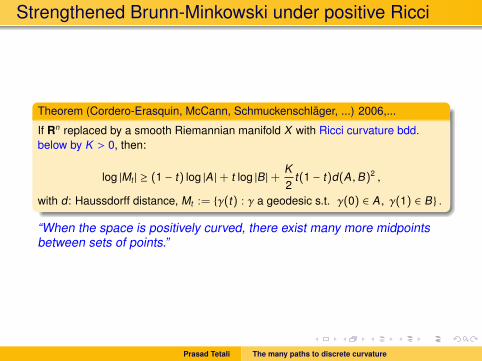
Theorem (Cordero-Erasquin, McCann, Schmuckenschlager, ...) 2006,...
If Rn replaced by a smooth Riemannian manifold X with Ricci curvature bdd.below by K > 0, then:
log |Mt | � (1 � t) log |A |+ t log |B |+ K2
t(1 � t)d(A ,B)2 ,
with d: Haussdorff distance, Mt := {�(t) : � a geodesic s.t. �(0) 2 A , �(1) 2 B} .
“When the space is positively curved, there exist many more midpointsbetween sets of points.”
Prasad Tetali The many paths to discrete curvature

Discrete Brunn-Minkowski type Inequality?
Definition. Graph G = (V ,E); for A ,B ⇢ V , for 0 t 1, letMt(A ,B) be the t-midpoint set of A and B. i.e., for a 2 A , b 2 B,
Mt(a, b) := {z 2 V(G) : d(a, z) ⇡ td(a, b), d(z, b) ⇡ (1 � t)d(a, b)} ,
E.g.,M1/2(a, b) := {m : d(a,m)+d(m, b) = d(a, b); d(a,m) = d(m, b)+ {�1, 0,+1}}and
Mt(A ,B) = [a2A ,b2B Mt(a, b) .
Ollivier-Villani (2012): Brunn-Minkowski type inequality on the discretehypercube ⌦n = {0, 1}n equipped with the Ham. distance d(x, y) =
Pni=1 1Ixi,yi .
|M1/2(A ,B)| � |A |1/2|B |1/2e1
16n d2(A ,B), 8A ,B ⇢ ⌦n
Above is a consequence of the following: 8⌫0, ⌫1, 9⌫1/2 such that
H(⌫1/2|µ) 12
H(⌫0|µ) +12
H(⌫1|µ) �1
16nW2
1 (⌫0, ⌫1),
where µ is the uniform measure on ⌦n.
Prasad Tetali The many paths to discrete curvature

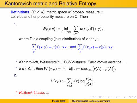
Kantorovich metric and Relative EntropyDefinitions. (⌦, d, µ): metric space w/ probab. measure µ.Let ⌫ be another probability measure on ⌦. Then
1.W1(⌫, µ) := inf
�!(⌫,µ)
X
x,y2⌦d(x, y)�(x, y) ,
where � is a coupling (joint distribution) of ⌫ and µ:X
y
�(x, y) = µ(x), 8x, andX
x
�(x, y) = ⌫(y), 8y .
* Kantorovich, Wasserstein, KROV distance, Earth mover distance, ...
* If d 2 0, 1, then W1(⌫, µ) = k⌫ � µktv := supA⇢⌦⇣⌫(A) � µ(A)
⌘.
2.
H(⌫|µ) :=X
x2⌦⌫(x) log
⌫(x)µ(x)
.
* Kullback-Liebler, ...
Prasad Tetali The many paths to discrete curvature
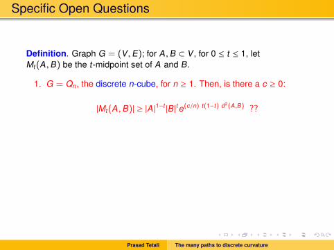
Specific Open Questions
Definition. Graph G = (V ,E); for A ,B ⇢ V , for 0 t 1, letMt(A ,B) be the t-midpoint set of A and B.
1. G = Qn, the discrete n-cube, for n � 1. Then, is there a c � 0:
|Mt(A ,B)| � |A |1�t |B |t e(c/n) t(1�t) d2(A ,B) ??
2. G = Sn, the symmetric group with the Hamming (or, say, thetransposition) distance defining adjacency. Then, is there a c � 0:
|Mt(A ,B)| � |A |1�t |B |t e(c/n) t(1�t) d2(A ,B) ??
* “Curvature” term ...
Prasad Tetali The many paths to discrete curvature
Ollivier-Villani
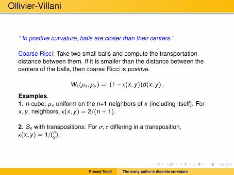
“ In positive curvature, balls are closer than their centers.”
Coarse Ricci: Take two small balls and compute the transportationdistance between them. If it is smaller than the distance between thecenters of the balls, then coarse Ricci is positive.
W1(µx , µy) =: (1 � (x, y))d(x, y) ,Examples.1. n-cube: µx uniform on the n+1 neighbors of x (including itself). Forx, y, neighbors, (x, y) = 2/(n + 1).
2. Sn with transpositions: For �, ⌧ differing in a transposition,(x, y) = 1/(n
2).
Prasad Tetali The many paths to discrete curvature

(Coarse) Ricci of Hypercube
Proposition (folklore)
The n-cube has coarse Ricci = 2/(n + 1).
Proof sketch.(i) Consider the lazy random walk on the n-cube.
(ii) Use a simple (path) coupling argument to show that two copies of thechain started at neighboring vertices x, y 2 {0, 1}n can be “coupled” withprobability at least 2/(n + 1) in one step.
Prasad Tetali The many paths to discrete curvature

(Coarse) Ricci of Transposition Graph
Proposition
Sn with transpositions has coarse Ricci = 1/(n2).
Proof sketch.Lower bound:(i) Consider the lazy random transposition chain on Sn.(ii) Use a simple (path) coupling argument to show that two copies of thechain started at �, ⌧ 2 Sn with d(�, ⌧) = 1, can be coupled withprobability at least 1/(n
2) in one step.
Upper bound: Follows by showing that there is no better coupling – use(Kantorovich’s) dual formulation of W1:
W1(⌫, µ) = supf : 1�Lip
✓E⌫f � Eµf
◆.
Prasad Tetali The many paths to discrete curvature
A general problem
(X, d) a complete separable metric space.
Definition [Relative entropy]
Let µ, ⌫ be two Borel probability measures on X
H(⌫|µ) :=Z
logd⌫dµ
d⌫
if ⌫ is absolutely continuous with respect to µ (otherwise we set H(⌫|µ) = 1).
The map ⌫ 7! H(⌫|µ) is always convex in the usual sense:
H((1 � t)⌫0 + t⌫1|µ) (1 � t)H(⌫0|µ) + tH(⌫1|µ), 8t 2 [0, 1].
Problem: Examine the convexity of H along other types of paths (⌫t)t2[0,1]interpolating between ⌫0 and ⌫1.
Convexity along geodesics of the Wasserstein W2 distance hasconnections with curvature of the underlying space and functional inequalities(Log-Sobolev, Talagrand) or Brunn-Minkowski type inequalities.
Prasad Tetali The many paths to discrete curvature

I. Displacement convexity of theentropy in a continuous setting.
Prasad Tetali The many paths to discrete curvature
Geodesic spaces
A metric space (E, d) is said geodesic if for all x0, x1 2 E there is at least one path� : [0, 1]! E such that �(0) = x0 and �(1) = x1 and
d(�(s), �(t)) = |t � s|d(x0, x1), 8t , s 2 [0, 1].
Such a path is called a constant speed geodesic between x0 and x1.
Prasad Tetali The many paths to discrete curvature

Geodesics in the Wasserstein space
Let Pp(X), p � 1, be the set of Borel probability measures having a finite p-thmoment.
Definition [Lp-Wasserstein distance]
Let ⌫0, ⌫1 2 Pp(X);
Wpp (⌫0, ⌫1) = inf
⇡2P(⌫0 ,⌫1)
"
dp(x0, x1) ⇡(dx0dx1),
where P(⌫0, ⌫1) is the set of couplings of ⌫0 and ⌫1.
Theorem
If p > 1, the space (Pp(X),Wp) is geodesic if and only if (X, d) is geodesic.
Prasad Tetali The many paths to discrete curvature

Displacement Convexity of Entropy
Theorem
Let (M, g) be a complete connected Riemannian manifold and suppose thatµ 2 P(M) is absolutely continuous with µ(dx) = e�V(x) dx. The following areequivalent:
1 µ verifies the CD(K ,1) condition, for some K 2 R:
Ric + Hess V � Kg
2 The relative entropy functional is K -displacement convex with respect to theW2 metric: for all ⌫0, ⌫1 2 P2(M), absolutely continuous with respect to µ,there is a W2-geodesic (⌫t)t2[0,1] connecting ⌫0 to ⌫1 such that
H(⌫t |µ) (1 � t)H(⌫0|µ) + tH(⌫1|µ) � Kt(1 � t)
2W2
2 (⌫0, ⌫1), 8t 2 [0, 1]
McCann, Cordero-McCann-Schmuckenschlager, Sturm-Von Renesse,Lott-Villani, Sturm.
Prasad Tetali The many paths to discrete curvature
Implications: Bakry-Emery etc.
1. This equivalence sets the ground for a possible definition of the conditionCD(K ,1) on geodesic spaces (Lott-Villani; Sturm).
2. Brunn-Minkowski type inequalities. Suppose K � 0, then
µ([A ,B]t) � µ(A)1�tµ(B)t eKt(1�t)
2 d2(A ,B), 8t 2 [0, 1],
where [A ,B]t = {x 2 M;9(a, b) 2 A ⇥ B , d(x, a) =(1 � t)d(a, b) and d(x, b) = td(a, b)}.
3. Talagrand’s inequality. Suppose K > 0, then
W22 (⌫0, µ)
2K
H(⌫0|µ), 8⌫0 2 P2(M).
4. HWI inequality. Otto-Villani, 2000.
Prasad Tetali The many paths to discrete curvature

5. Log-Sobolev inequality. Suppose K > 0, then
H(⌫0|µ) 2K
I(⌫0|µ), 8⌫0.
6. Prekopa-Leindler type inequalities. Suppose K 2 R, and fix t 2 (0, 1).If f , g, h : M ! R are such that
h(z) � (1 � t)f(x) + tg(y) � Kt(1 � t)2
d2(x, y), 8x, y 2 M, z 2 [x, y]t
then Zeh(z) µ(dz) �
Zef(x) µ(dx)
!1�t Zeg(y) µ(dy)
!t
Prasad Tetali The many paths to discrete curvature
II. Displacement convexity of theentropy in a discrete setting.
Prasad Tetali The many paths to discrete curvature
Extension to discrete settings
Question: Is it possible to extend this theory to discrete settings, for examplefinite graphs ?
Two obstructions:
Talagrand’s inequality
W22 (⌫0, µ) Const. H(⌫0|µ), 8⌫0
does not hold in discrete setting unless µ is a Dirac.
W2-geodesics do not exist in discrete setting; even on a two-point space!
W2 is not adapted neither for defining the path ⌫t nor for measuring theconvexity defect/excess of the entropy.
Prasad Tetali The many paths to discrete curvature

..., Schmuckenschlager, Chung-Yau, Sammer-T., Ollivier, Ollivier-Villani,Bonciocat-Sturm, Maas, Chow-Huang-Li-Zhou, Erbar-Maas,Gozlan-Roberto-Samson-T., Mielke, Hillion, Leonard, Lehec, Joulin, Veysseire,Bauer et al, Klartag et al, Munch, . . .
Prasad Tetali The many paths to discrete curvature

The various paths to curvature...
Dobrushin, Sammer, ..., Ollivier: W1 contraction approach
M. Erbar, J. Maas; S-N. Chow, W. Huang, Y. Li, H-M. Zhou: Displacementconvexity of entropy using interpolation along newW2 geodesic, a PDEapproach, where the geodesics minimize certain kinetic energy intransporting one density (of molecules) to another.
N. Gozlan, C. Roberto, P-M. Samson, P.T.: Displacement convexity ofentropy using interpolation along W1 geodesics, a probabilistic approach.
Schmuckenschlager, Klartag-Kozma-Ralli-P.T.:Discrete versions of the Bochner formula, the so-called �2 criterion,comparing the 2nd derivative (of the variance/entropy of the heat flow) withthe first derivative...
Bauer-Horn-Lin-Lippner-Mangoubi-S.T.Yau:“Li-Yau Inequality on Graphs” : a local notion of curvature-dimensioninequality with some consequences
Prasad Tetali The many paths to discrete curvature

The various paths to curvature...
Dobrushin, Sammer, ..., Ollivier: W1 contraction approach
N. Gozlan, C. Roberto, P-M. Samson, P.T.: Displacement convexity ofentropy using interpolation along W1 geodesics, a probabilistic approach.
Schmuckenschlager, Klartag-Kozma-Ralli-P.T.:Discrete versions of the Bochner formula, the so-called �2 criterion,comparing the 2nd derivative (of the variance/entropy of the heat flow) withthe first derivative...
Bauer-Horn-Lin-Lippner-Mangoubi-S.T.Yau:“Li-Yau Inequality on Graphs” : a local notion of curvature-dimensioninequality with some consequences
M. Erbar, J. Maas; S-N. Chow, W. Huang, Y. Li, H-M. Zhou: Displacementconvexity of entropy using interpolation along newW2 geodesic, a PDEapproach, where the geodesics minimize certain kinetic energy intransporting one density (of molecules) to another.
Prasad Tetali The many paths to discrete curvature

Interpolation along W1-geodesics : Gozlan,Roberto, Samson, and T.
Prasad Tetali The many paths to discrete curvature

GRST approach
similar approach developed independently by E. Hillion
Definition [L1-Wasserstein distance]
For all ⌫0, ⌫1 2 P(V), W1(⌫0, ⌫1) = inf⇡2P(⌫0 ,⌫1)
!
d(x0, x1) ⇡(dx0dx1).
We seek to prove convexity of the entropy along (pseudo)-W1-geodesics ⌫t
connecting ⌫0 to ⌫1 :
There is some K � 0 such that for all ⌫0, ⌫1 there is some pseudo W1-geodesic ⌫t
connecting ⌫0 to ⌫1 such that for all t 2 [0, 1]
H(⌫t |µ) (1 � t)H(⌫0|µ) + tH(⌫1|µ) �Kt(1 � t)
2⇥ · · · .
A good candidate for the transport term in the right hand side is W21 (⌫0, ⌫1) .
Prasad Tetali The many paths to discrete curvature

Our main example - the discrete hypercube ⌦n
Theorem [GRST]
Let µ be a probability on {0, 1} and denote by µn its n-fold tensor product. Thefollowing displacement convexity properties of the entropy hold true.
For all ⌫0, ⌫1 2 P(⌦n), there is a coupling ⇡ 2 P(⌫0, ⌫1) such that for all t 2 [0, 1], itholds
H(⌫⇡t |µn) (1 � t)H(⌫0|µn) + tH(⌫1|µn) � 2t(1 � t)n
W21 (⌫0, ⌫1)
where⌫⇡t =
X
x0 ,x12⌦n
⇡(x0, x1)X
z2Jx0 ,x1Ktd(x0 ,z)(1 � t)d(z,x1)�z ,
where z 2 Jx0, x1K means that z belongs to some geodesic joining x0 to x1.
Prasad Tetali The many paths to discrete curvature
W1-geodesics
Definition [L1-Wasserstein distance]
For all ⌫0, ⌫1 2 P(V), W1(⌫0, ⌫1) = inf⇡2P(⌫0 ,⌫1)
!
d(x0, x1) ⇡(dx0dx1).
Important example:Let V = {0, 1, . . . , n}; consider the Binomial distribution B(n, t) defined by
B(n, t) =nX
k=0
nk
!tk (1 � t)n�k�k 2 P(V).
Then (B(n, t))t2[0,1] is a W1 constant-speed geodesic connecting �0 to �n.
Prasad Tetali The many paths to discrete curvature

Implications (Discrete Setting)
Displacement convexityw + u
Prekopa-Leindler + HWIu + w
Modified log-Sob Weak transport+
log-Sob for the Gaussian
Prasad Tetali The many paths to discrete curvature
Bochner formula (iterated gradient �2 criterion) :application: discrete Buser ...
Prasad Tetali The many paths to discrete curvature
Bakry-Emery, ... ,Schmuckenschlager,..., Klartag-KozmaG = (V ,E), and Graph Laplacian � = �(D � A)
Definition [Bochner w/ parameter K]
Curvature of G is at least K , if 8f : V ! R, and 8x 2 V ,
��(f , f)(x) � 2�(f ,�f)(x) � K �(f , f)(x) ,
where�f(x) =
X
y:(x,y)2E(f(y) � f(x)) .
And given f , g : V ! R, also define:
�(f , g)(x) =12
X
y:(x,y)2E(f(x) � f(y))(g(x) � g(y)) .
Note: When f = g, we get the more commonly denoted (square of the l2-type)discrete gradient: for each x 2 V ,
�(f)(x) := �(f , f)(x) =12
X
y:(x,y)2E(f(x) � f(y))2 =: |rf(x)|2 .
Prasad Tetali The many paths to discrete curvature

�2 Calculus
Equivalently ...
Curvature of G is at least K , if 8f : V ! R, and 8x 2 V ,
�2(f)(x) � K �(f)(x) ,
where�2(f) := �2(f , f) =
12��(f) � �(f ,�f) .
Basically, using the iterated gradient:
2�2(f , g) = ��(f , g) � �(f ,�g) � �(�f , g) .
Prasad Tetali The many paths to discrete curvature

�2 Calculus
Equivalently ...
Curvature of G is at least K , if 8f : V ! R, and 8x 2 V ,
�2(f)(x) � K �(f)(x) ,
where�2(f) := �2(f , f) =
12��(f) � �(f ,�f) .
Basically, using the iterated gradient:
2�2(f , g) = ��(f , g) � �(f ,�g) � �(�f , g) .
Prasad Tetali The many paths to discrete curvature

�2 Calculus
Equivalently ...
Curvature of G is at least K , if 8f : V ! R, and 8x 2 V ,
�2(f)(x) � K �(f)(x) ,
where�2(f) := �2(f , f) =
12��(f) � �(f ,�f) .
Basically, using the iterated gradient:
2�2(f , g) = ��(f , g) � �(f ,�g) � �(�f , g) .
Prasad Tetali The many paths to discrete curvature

�2 Calculus (contd.)
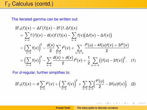
The iterated gamma can be written out:
2�2(f)(x) = ��(f)(x) � 2�(f ,�f)(x)
=X
v⇠x
�(f)(v) � d(x)�(f)(x) �X
v⇠x
f(v)⇣�f(v) ��f(x)
⌘
=✓X
v⇠x
f(v)◆2� d(x)
2
X
v⇠x
f2(v) +X
u⇠v⇠x
f2(u) � 4f(u)f(v) + 3f2(v)2
=✓X
v⇠x
f(v)◆2�
X
v⇠x
d(x) + d(v)2
f2(v) +12
X
u⇠v⇠x
⇣(f(u) � 2f(v)
⌘2. (1)
For d-regular, further simplifies to:
2�2(f)(x) = dX
v⇠x
f2(v) +✓X
v⇠x
f(v)◆2
+X
v⇠x
X
u⇠v
✓ f2(u)2� 2f(u)f(v)
◆. (2)
Prasad Tetali The many paths to discrete curvature

�2 Calculus (contd.)
The iterated gamma can be written out:
2�2(f)(x) = ��(f)(x) � 2�(f ,�f)(x)
=X
v⇠x
�(f)(v) � d(x)�(f)(x) �X
v⇠x
f(v)⇣�f(v) ��f(x)
⌘
=✓X
v⇠x
f(v)◆2� d(x)
2
X
v⇠x
f2(v) +X
u⇠v⇠x
f2(u) � 4f(u)f(v) + 3f2(v)2
=✓X
v⇠x
f(v)◆2�
X
v⇠x
d(x) + d(v)2
f2(v) +12
X
u⇠v⇠x
⇣(f(u) � 2f(v)
⌘2. (1)
For d-regular, further simplifies to:
2�2(f)(x) = dX
v⇠x
f2(v) +✓X
v⇠x
f(v)◆2
+X
v⇠x
X
u⇠v
✓ f2(u)2� 2f(u)f(v)
◆. (2)
Prasad Tetali The many paths to discrete curvature

Cheeger is tight under non-negative curvature!h := h(G) := minA⇢V |@A |/|A |, the Cheeger const, of G; � > 0 spectralgap of G.
Theorem (A-M, L-S, J-S 80’s)
h2
c1 maxdeg(G) � c2h .
Theorem (Klartag-Kozma-Ralli-T. ’14)
1. Bochner w/ parameter K implies: for any subset A ⇢ V,
|@A | � 12
min⇢p
�,�p2|K |
�|A |
✓1 � |A ||V |
◆.
2. Bochner w/ parameter K � 0 implies � � K, and hence:
� 16h2 .
3. Abelian Cayley graphs satisfy Bochner w/ parameter K � 0.
Prasad Tetali The many paths to discrete curvature

CD(K, 1) with K � 0: Examples
1. Complete graph Kn: Curvature = 1 + n/2.
2. Discrete n-cube Qn: Curvature = 2.
3. Symmetric group S(n) with the transposition metric: Curvature = 2
4. General Proposition. If T is the maximum number of trianglescontaining any edge, then K 2 + T/2.
5. Abelian necessary! On Sn, the (left) Cayley graph generated by(12), (12...n) ± 1, the Cheeger constant is c1n�2, while the spectral gap isc2n�3, with c1, c2 > 0, independent of n.
Prasad Tetali The many paths to discrete curvature

Cheeger, CD(K, 1) with K � 0
Qn. 1 Can we characterize the graphs or Markov kernels which satisfynon-negative curvature?
Qn. 2 Can we characterize the graphs for which the Cheeger inequality istight?
Qn. 3 More examples? Non-crossing partition lattice NC(n)?
Prasad Tetali The many paths to discrete curvature
Erbar-Maas:
X : finite set;K : X ⇥ X! R+ : irreducible Markov kernel;⇡ : the unique invariant probab. measure for K .
Let
P(X) :=⇢⇢ : X! R+ |
X
x2X⇡(x)⇢(x) = 1
�
and let P+(X) ⇢ P(X) be the subset consisting of strictly positive probabilitydensities on X.
Given ⇢ 2 P(X), recall the logarithmic mean of ⇢(x) and ⇢(y):
• ⇢(x, y) := ✓⇣⇢(x), ⇢(y)
⌘:=
Z 1
0⇢(x)1�p⇢(y)pdp =
⇢(x) � ⇢(y)log ⇢(x) � log ⇢(y)
.
• H(⇢) =P
x2X ⇡(x)⇢(x) log ⇢(x) .
Prasad Tetali The many paths to discrete curvature

Displacement Convexity and Ricci a la Maas
Definition (Maas)
Now consider the metricW defined for ⇢0, ⇢1 2 P(X) by
W(⇢0, ⇢1)2 := inf
⇢,
(12
Z 1
0
X
x,y2X( t(x) � t(y))2⇢t(x, y)K(x, y)⇡(x)dt
),
where the infimum runs over all sufficiently regular curves ⇢ : [0, 1]! P(X) and : [0, 1]! RX satisfying the continuity equation
8>>>><>>>>:
ddt⇢t(x) +
X
y2X( t(y) � t(x))⇢t(x, y)K(x, y) = 0 8x 2 X ,
⇢(0) = ⇢0 , ⇢(1) = ⇢1 .
(3)
Definition (Maas)
Markov kernel K has Ricci curvature bounded from below by 2 R, if for anyconstant-speed geodesic {⇢t }t2[0,1] in (P(X),W), we have
H(⇢t) (1 � t)H(⇢0) + tH(⇢1) �
2t(1 � t)W(⇢0, ⇢1)
2 .
Prasad Tetali The many paths to discrete curvature

The PDE approach
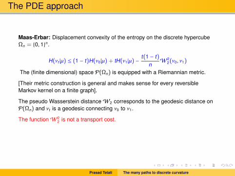
Maas-Erbar: Displacement convexity of the entropy on the discrete hypercube⌦n = {0, 1}n.
H(⌫t |µ) (1 � t)H(⌫0|µ) + tH(⌫1|µ) �t(1 � t)
nW2
2(⌫0, ⌫1)
The (finite dimensional) space P(⌦n) is equipped with a Riemannian metric.
[Their metric construction is general and makes sense for every reversibleMarkov kernel on a finite graph].
The pseudo Wasserstein distanceW2 corresponds to the geodesic distance onP(⌦n) and ⌫t is a geodesic connecting ⌫0 to ⌫1.
The functionW22 is not a transport cost.
This implies some versions of LSI and HWI, and a Talagrand typeinequality for theW2 and W1 distances with sharp constants.
Prasad Tetali The many paths to discrete curvature
The PDE approach
Maas-Erbar: Displacement convexity of the entropy on the discrete hypercube⌦n = {0, 1}n.
H(⌫t |µ) (1 � t)H(⌫0|µ) + tH(⌫1|µ) �t(1 � t)
nW2
2(⌫0, ⌫1)
The (finite dimensional) space P(⌦n) is equipped with a Riemannian metric.
[Their metric construction is general and makes sense for every reversibleMarkov kernel on a finite graph].
The pseudo Wasserstein distanceW2 corresponds to the geodesic distance onP(⌦n) and ⌫t is a geodesic connecting ⌫0 to ⌫1.
The functionW22 is not a transport cost.
This implies some versions of LSI and HWI, and a Talagrand typeinequality for theW2 and W1 distances with sharp constants.
Prasad Tetali The many paths to discrete curvature

Ricci vs Coarse Ricci Curvature
Theorem (M.Erbar-J.Maas-P.T.)1. k -slice of the n-cube (with 1-0 transpositions) has Ricci =⇥(n/[k(n � k)]) ;
2. Sn with transpositions has Ricci = ⌦(1/n2) .
Conjecture
Sn with transpositions has Ricci = ⌦(1/n).
Remark. It can not be better than (1/n), since both the spectral gap andthe modified Log-Sobolev (entropy) constant are ⇥(1/n), and these areimplied by (the stronger notions of) Ricci – e.g., those of Erbar-Maas andGozlan-Roberto-Samson-T.
Prasad Tetali The many paths to discrete curvature

Collaboration Acknowledgment
N. Gozlan, C. Roberto, P-M. Samson, P. Tetali, “Dispalcement Convexity inGraphs and Related Inequalities,” Probab. Th. Rel. Fields, 2013.
M. Erbar, J. Maas, P. Tetali, “Discrete Ricci Curvature bounds forBernoulli-Laplace and the Random Transposition Models,” Annales Fac.Sci. Toulouse, 2015.
R. Che, W. Huang, Y. Li, P. Tetali, “Convergence to Global Equilibrium inFokker-Planck Equations on a Graph and Talagrand-type inequalities,” J.Diff. Equations, 2016.
B. Klartag, G. Kozma, P. Ralli, P. Tetali, “Discrete Curvature and AbelianGroups,” Canadian J. Math., 2016.
N. Gozlan, C. Roberto, P-M. Samson, P. Tetali, “Kantorovich Duality forgeneral Transport Costs and Applications,” J. Functional Analysis, accepted.
M. Erbar, C. Henderson, G. Menz, P. Tetali, “Ricci Curvature bounds forWeakly Interacting Markov Chains,” Electronic J. Probab., 2017.
Prasad Tetali The many paths to discrete curvature

Thank you!
Prasad Tetali The many paths to discrete curvature

Back to the Cube: Kruskal-Katona consequence
Let A ⇢ {0, 1}n, B := 0 (singleton); let d = 1|A |
Pa2A d(0, a) . Then
Proposition
|Mt(0,A)|2 � t2|A |t et log(1/t) d2
.
Proof idea. We may use a theorem of Lovasz:If |A | = (x
m), for some x 2 R, then its shadow has size, |@A | � ( xm�1) .
Idea: write A as the (disjoint) union of its intersection with the level-sets,and use the observation: Mj/m(0,Am) = @m�jAm , for 0 j m.
Prasad Tetali The many paths to discrete curvature
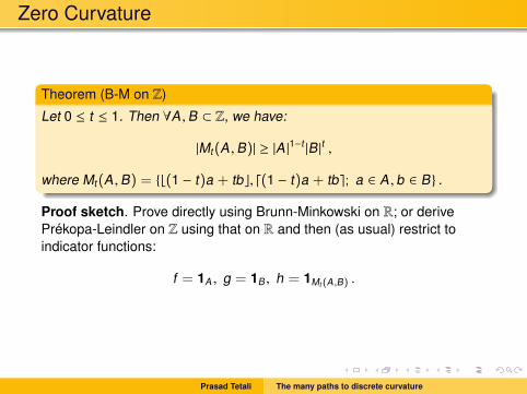
Zero Curvature
Theorem (B-M on Z)Let 0 t 1. Then 8A ,B ⇢ Z, we have:
|Mt(A ,B)| � |A |1�t |B |t ,
where Mt(A ,B) = {b(1 � t)a + tbc, d(1 � t)a + tbe; a 2 A , b 2 B} .
Proof sketch. Prove directly using Brunn-Minkowski on R; or derivePrekopa-Leindler on Z using that on R and then (as usual) restrict toindicator functions:
f = 1A , g = 1B , h = 1Mt (A ,B) .
Prasad Tetali The many paths to discrete curvature

Zero Curvature (contd.)
Theorem (P-L on Z)
Let 0 t 1. If f , g, h : Z! R+, s.t. we have:
h(m) � f(a)1�t g(b)t , 8a, b 2 Z , and m 2 Mt(a, b) ,
then we also have:X
m2Zh(m) �
✓X
a2Af(a)
◆1�t✓X
b2Bg(b)
◆t.
Proof sketch. Apply the classical continuous Prekopa-Leindler to thefunctions:
f(x) = f(bx + 1/2c), g(x) = g(bx + 1/2c), h(x) = h(bx + 1/2c), x 2 R .
The hypothesis can be verified for these functions by checking that:
m := b(1 � t)x + ty + 1/2c 2 Mt(bx + 1/2c, by + 1/2c) .
Prasad Tetali The many paths to discrete curvature

Continuing with the Integers
1. (J. Melbourne). Previous result can be extended to Z mod n.
2. (K. Costello, P.T.): The t = 1/2 case of Z (and Z mod p) can behandled with the Cauchy-Davenport sumset inequality!
Prasad Tetali The many paths to discrete curvature

Sn : midpoint injection
Theorem (K. Costello, P.T.)Consider the transposition graph on Sn, with d being the transpositiondistance. Then, for all A ,B ⇢ Sn, we have
|M1/2(A ,B)|2 � |A ||B | .
Proof sketch. Consider a 2 A and b 2 B be so that d(a, b) = d.
Let M1(a, b) be the set of perms. of distance bd/2c from a and distancedd/2e from b, and
M2(a, b) be the set of perms. of distance dd/2e from a and distancebd/2c from b.
define canonical paths between a 2 A and b 2 B and exhibit an injectionfrom A ⇥ B to M1 ⇥M2.
Prasad Tetali The many paths to discrete curvature

Sn : a canonical path construction
Towards an injection from A ⇥ B to M1 ⇥M2:
• Factorize ba�1 = td td�1 . . . t1 as a product of d transpositions (from rightto left):
i) If ba�1 is a single cycle, write it as (a1a2 · · · ak ), where ak < ai for alli , k . Then factorize the cycle as (a1a2)(a2a3) . . . (ak�1ak ).
ii) If it consists of several cycles, sort the cycles in decreasing order bythe smallest element in each cycle, then concatenate the factorizationsfor each cycle.
• Define x = tbd/2c · · · t1 and y = td · · · t1+bd/2c. Then define
m1 := xa and m2 := x�1yxa = x�1b .
Thus given m1 and m2, we know x�1y = m2m�11 .
Prasad Tetali The many paths to discrete curvature

Sn : path argument (contd.)
• Define x = tbd/2c · · · t1 and y = td · · · t1+bd/2c. Then define
m1 := xa and m2 := x�1yxa = x�1b .
Thus given m1 and m2, we know x�1y = m2m�11 .
Claim (near commutativity of x and y). Any two elements are in the samecycle in x�1y iff they are in the same cycle in yx.
Prasad Tetali The many paths to discrete curvature

Sn : injection completed
Claim (near commutativity of x and y). Any two elements are in the samecycle in x�1y iff they are in the same cycle in yx.
• Using the claim, knowing the cycles of x�1y, we will know the cycles ofyx, and hence the distance d.• By the (canonical) path construction, we may know which cycles arepart of x and which are part of y, and which cycle (if any) is split!Furthermore, we know where in the (shared) cycle the split occurred,since we know d and which cycles are from x.
Thus we may recover x and y and hence also a and b, given m1 and m2.
Prasad Tetali The many paths to discrete curvature


![Discrete Morse theory and classifying spacespeople.maths.ox.ac.uk/nanda/source/discrete_CJSX.pdf · theory [10,11]. It would be interesting if the theory of flow paths developed](https://img.dokumen.tips/doc/110x75/5edc26b8ad6a402d6666b1fc/discrete-morse-theory-and-classifying-theory-1011-it-would-be-interesting-if.jpg)