1

The Malthusian Model

I. Introduction

After reviewing the key development and growth facts, it is clear

that we need a theory that can generate a period of constant living

standards, followed by a transition period with modest increases in

living standards, followed by a period of modern economic growth.

We already have a model that can account for the period of modern

economic growth; the Solow Model with technological change

generates constant growth of per capita output.

It is true that the Solow Model can generate a steady state with a

constant level of per capita output as long as there is no exogenous

technological change. One possibility, therefore, is to interpret the

pre-1700 era of constant livings standards as the steady state of the

Solow Model absent technological change. The problem with this

interpretation is that technology was not stagnant before 1700. Joel

Mokyr a noted economic historian at Northwestern University

documents in his book The Lever of Riches the large number of

important technological innovations that preceded the eighteenth

century.

Thomas Malthus-1776-1834

Who was Thomas Malthus?

Thomas Malthus was a professor of History and Political Economy at the East India Company College at Hertfordshire. Although his students affectionately referred to him as “PoP” or “Population Malthus”, he could have easily been called Professor gloom on the dire implication of his theory that population growth would outstrip food growth, causing a check on the population. His influence went far beyond the political and economic debates of his time. Both Charles Darwin and Alfred Russell Wallace credited Malthus for helping them develop the theory of Natural Selection.

Thomas Malthus was also a cleric in the Church of England, and some of his religious views are evident in his economic views. For instance, he viewed the limits to population growth to be a divine phenomenon that was to be used to teach virtue across society, particularly the lower classes.

2

In light of the historical record on technological change, we develop an alternative theory

and model of this pre-1700 era. This is the Malthusian model that goes back to David

Ricardo, Thomas Malthus and other classical economists. There are really two key

components to the model. The first is the production process. This part of the model

relies heavily on the work of David Ricardo. Although as in the Solow model, the

production function is characterized by constant returns to scale and the law of

diminishing returns applies with respect to each factor input, importantly, in the

Malthusian model one of these factors is fixed in supply, namely, its quantity cannot be

changed over time. The common convention is to assume production requires capital,

labor and land inputs, with land being the factor whose supply cannot be changed over

time. The second key component is a population growth function that is an increasing

function of per capita consumption. This part of the model is based on the work of

Thomas Malthus. Together, these two elements ensure that the steady state is

characterized by a constant living standard and positive population growth even when

there is technological change.

We proceed by first presenting the Malthusian model with no capital and absent

technological change to help develop intuition for the full scale model. A virtue of this

version of the model is that the steady state equilibrium can be solved graphically. We

then add capital and exogenous technological change to the model. Having capital in the

model is not essential to generating a steady state with a constant living standard.

However in the later chapters when we combine the Malthus and Solow models, we will

need this feature and so we add it now to the Malthusian model rather than later.

3

Although graphical analysis is sufficient for understanding the Malthusian model without

technological change and capital, it is not so when we add technological change and

saving. Thus, solving for the steady state for the full model is done so algebraically.

II. Model with No Capital or Technological Change

People. Initially, there are N0 people alive. We use Nt to denote the number of people in

the economy at date t. People prefer more consumption to less.

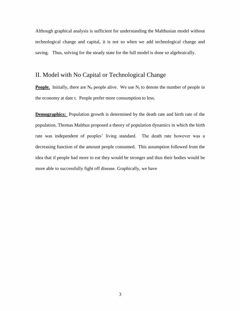
Demographics: Population growth is determined by the death rate and birth rate of the

population. Thomas Malthus proposed a theory of population dynamics in which the birth

rate was independent of peoples’ living standard. The death rate however was a

decreasing function of the amount people consumed. This assumption followed from the

idea that if people had more to eat they would be stronger and thus their bodies would be

more able to successfully fight off disease. Graphically, we have

4

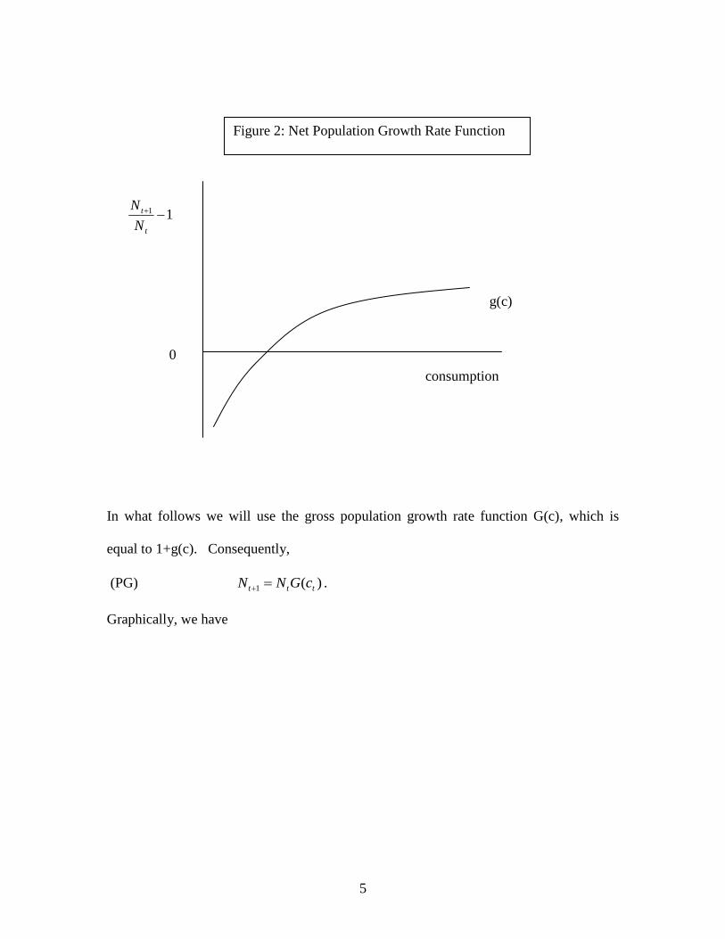
The population growth rate for a given level of consumption is the difference between the

birth rate and the death rate. We denote this function by g(c). When the birth rate equals

the death rate, the population does not change, namely Nt+1=Nt. More generally,

Nt+1=Nt[1+g(c)]. This is shown in Figure 2.

consumption

Birth rate

death rate

Figure 1: Birth and Death Rates as

functions of per capita consumption

5

In what follows we will use the gross population growth rate function G(c), which is

equal to 1+g(c). Consequently,

(PG) )(1 ttt cGNN .

Graphically, we have

consumption

11

t

t

N

N

Figure 2: Net Population Growth Rate Function

0

g(c)

6

Endowments: Each person in the economy is endowed with one unit of time each period

which he or she can use to work. Additionally, individuals own an equal share of the

land, which is fixed in quantity at L. Land does not depreciate. The per capita

endowment is thus, L/Nt.

consumption

Figure 3: Gross Population Growth Rate Function

1

G(c)

t

t

N

N 1

7

Production Function: The economy produces a single final good using labor and land.

The production function is given by

(Y) 1

ttt NLAY

The letter A is again the Total Factor Productivity (TFP).

Notice that this production function looks the same as the production function in the

Solow model except that (1-α) is labor’s share and instead of capital we have land as the

second input. The production function is still characterized by constant returns to scale,

and is increasing in each of its two input. Moreover, the law of diminishing returns

applies to each factor separately; the increases in output associated with an additional unit

of labor input decrease as labor increases holding the land input fixed.

The key feature, however, is that land is essential in production, and that the supply of

land is fixed. Thus, there is no way that you can double total output if you double the

population because the quantity of land cannot be changed.

General Equilibrium:

There are three markets that must clear in each period for the economy to be equilibrium:

the labor market, the land rental market, and the goods market. Equilibrium quantities

are trivially determined in this model, as they were in the Solow Growth model. This is

because the supply of labor and the supply of land are both vertical; people supply their

entire time endowment to the market and their entire land endowment to the market. As

Nt and L are the equilibrium inputs, it is trivial to determine the equilibrium amount of

8

output. This is 1

ttt NLAY . For the goods market to clear we simply require that all

output is consumed,

(C) Ntct=Yt.

This is the case as there is no capital in the model. Equation (C) is the consumption

equation.

The equilibrium prices are the rental price of land rLt and the real wage rate, wt. To

determine these we need to use the firm’s labor demand and its demand for land services.

Once again, these are the marginal product of land and the marginal product of labor.

These follow from the profit maximization problem of the firm. This is

(Profits) tLttttt LrNwNLA 1

(LD) t

tttt

N

YNLAw )1()1(

(LnD) t

tttLt

L

YNLAr 11

Steady State Analysis

We begin with characterizing the steady state equilibrium. First, note that there cannot be

sustained growth in per capita output or consumption in this model. The reason for this is

that the only way a person’s output could be increased is by increasing the amount of

land he uses. However, land is fixed and so it cannot be increased on a per person basis.

Thus, a steady state equilibrium is characterized by a constant path of per capita

consumption and per capita output, i.e. zero growth. Once we recognize this fact, it must

be the case that the population is constant in a steady state. Otherwise, with diminishing

9

returns, per capita output and per capita consumption would have to fall as we add more

people to work the land.

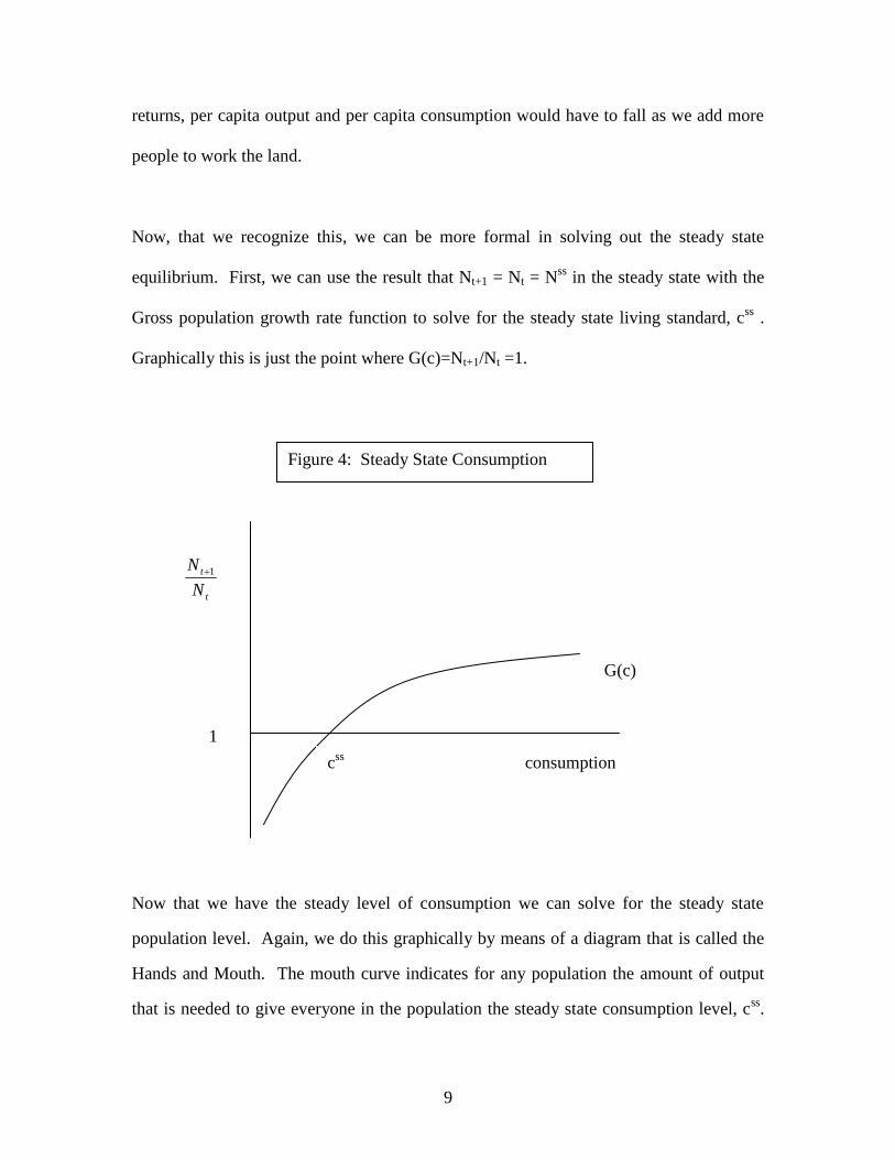
Now, that we recognize this, we can be more formal in solving out the steady state

equilibrium. First, we can use the result that Nt+1 = Nt = Nss

in the steady state with the

Gross population growth rate function to solve for the steady state living standard, css

.

Graphically this is just the point where G(c)=Nt+1/Nt =1.

Now that we have the steady level of consumption we can solve for the steady state

population level. Again, we do this graphically by means of a diagram that is called the

Hands and Mouth. The mouth curve indicates for any population the amount of output

that is needed to give everyone in the population the steady state consumption level, css

.

consumption

Figure 4: Steady State Consumption

1

G(c)

t

t

N

N 1

css

10

This is just a straight line from the origin with slope, css

. The hands curve is the amount

of output that is produced with a given population size. This is just the production

function curve. The steady state population is determined by the intersection of these two

curves. This is shown below.

1NALY

N

Figure 5: Steady State Population

Ntcss

Nss

Mouth

Hands

11

Algebraically, what we have done in solving for the steady state is first use the population

growth rate function to solve for css

when Nt+1/Nt=1. This is )(1 sscG . The next step,

which uses the hands and mouth graph, is to solve for Nss

using the goods market clearing

condition and the production function equation. Namely, 1NALNc ss . The left hand

side of the goods market clearing condition is the mouth curve while the right hand side

is the hands.

Comparative Statics

We can use the population growth function diagram and the hands-mouth diagram to

show how the steady state of the economy is affected by various factors. As the birth and

death rates determine the function G(c), anything that affects either of these two curves

affects the steady state consumption level and population by changing the position of the

mouths curve. Anything that changes the production function will change the steady

state population through its effect on the Hands curve. The production function change

will not have any effect on the steady state consumption level, however, as it is

determined exclusively by the birth and death rate curves.

To illustrate, suppose for example, there is an increase in the death rate, say caused by a

new strain of virus. How will this affect the economy’s living standard, and population?

The analysis always starts with the birth and death rate curves. We ask the question if the

proposed even causes a change in either of these two curves? The answer is clearly yes;

the new virus strain will increase the death rate for any given level of consumption,

namely, the d curve shifts up. With an increase in the death rate curve, the population

function curve G will decrease, implying an increase in the steady state level of

consumption. Moving on to the Hands and Mouth Diagram, this implies an increase in

12

the slope of the mouth curve, which in turn implies a decrease in the steady state

population. Thus, a permanent increase in the death rate is associated with fewer, but

richer people in the country.

Consider next an increase in TFP or the quality of Land. If there is an increase in TFP or

the quality of land, then there is no effect of the birth rate, death rate, or growth rate

function and hence no change in the steady state consumption level. There is no shift in

the Mouth curve then. The increase in TFP or the quality of land does shift the Hands

curve upward, which translates into a higher steady state population level. This is shown

in the below curve.

consumption

Birth rate

death rate

Figure 6: Increase in Death rate

13

Transitional Dynamics

Recall, for an economy to be on its steady state it must start out with the right initial

conditions. In the case of the Malthus model, this initial condition is in terms of the

population size. A steady state requires that the economy begin with N0=Nss

. As in our

study of the Solow model, we ask what happens if the economy does not start with the

right initial conditions. Will it converge to the steady state both in terms of consumption

and population? The answer is yes, it will. This can be seen by using the Hands and

Mouth Diagram.

Suppose an economy starts with a population below the steady state level. According to

the Hands equation, output is at Y0. The Mouth equation tells us the amount of output

needed to give each person the steady state consumption level. It is clear that total output

exceeds the required amount. Hence, c0 > css

. Now consider what happens to population

in period 1. Here we use the population growth function. As c0 > css

, the population

growth function implies that N1/N0 > 1, so population expands. Now at N1, it is still the

case that the Hands output exceeds the Mouth output, so that the living standard, c1>css

.

1NALY

N

Figure 7: Increase in TFP

Ntcss

Nss

14

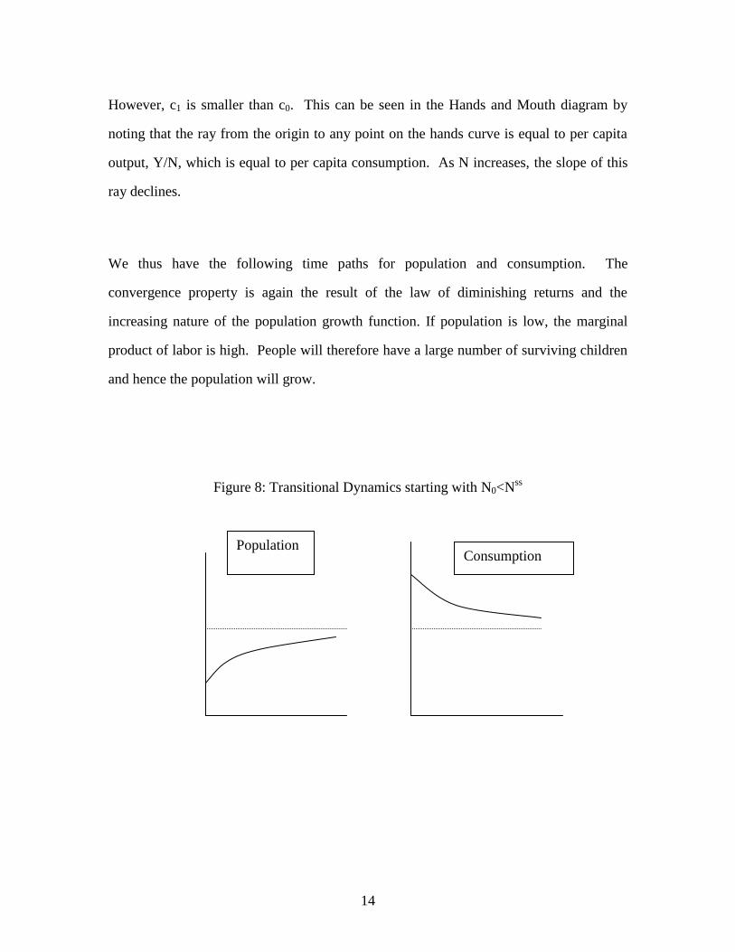
However, c1 is smaller than c0. This can be seen in the Hands and Mouth diagram by

noting that the ray from the origin to any point on the hands curve is equal to per capita

output, Y/N, which is equal to per capita consumption. As N increases, the slope of this

ray declines.

We thus have the following time paths for population and consumption. The

convergence property is again the result of the law of diminishing returns and the

increasing nature of the population growth function. If population is low, the marginal

product of labor is high. People will therefore have a large number of surviving children

and hence the population will grow.

Figure 8: Transitional Dynamics starting with N0<Nss

Population Consumption

15

Empirical Support for Malthus

Before we turn to the extension of the model with capital and technological change, it is

useful to take a step back and ask whether the historical evidence supports the predictions

of the model. Yes, there is the prediction that the living standard is constant, but there are

other predictions that can be checked with the historical record.

Recall that an increase in either A or L will have the same effect; neither changes the

population growth function, and hence the steady state consumption, but each does

increase the Hands curve, which results in a larger population. This prediction is borne

out by the data. Researchers such as Oded Galor (2011 Table 3.2 and Figure 3.5) have

shown that conditioning on a number of factors, countries with a higher land productivity

had higher population densities in 1500. The results come from a cross-country

regression with population density as the dependent variable. Land productivity is a

measure that is based on the amount of arable land, soil quality and temperature.

The behavior of the English economy from the second half of the 13th

century until nearly

1800 is described well by the Malthusian model. Real wages and, more generally, the

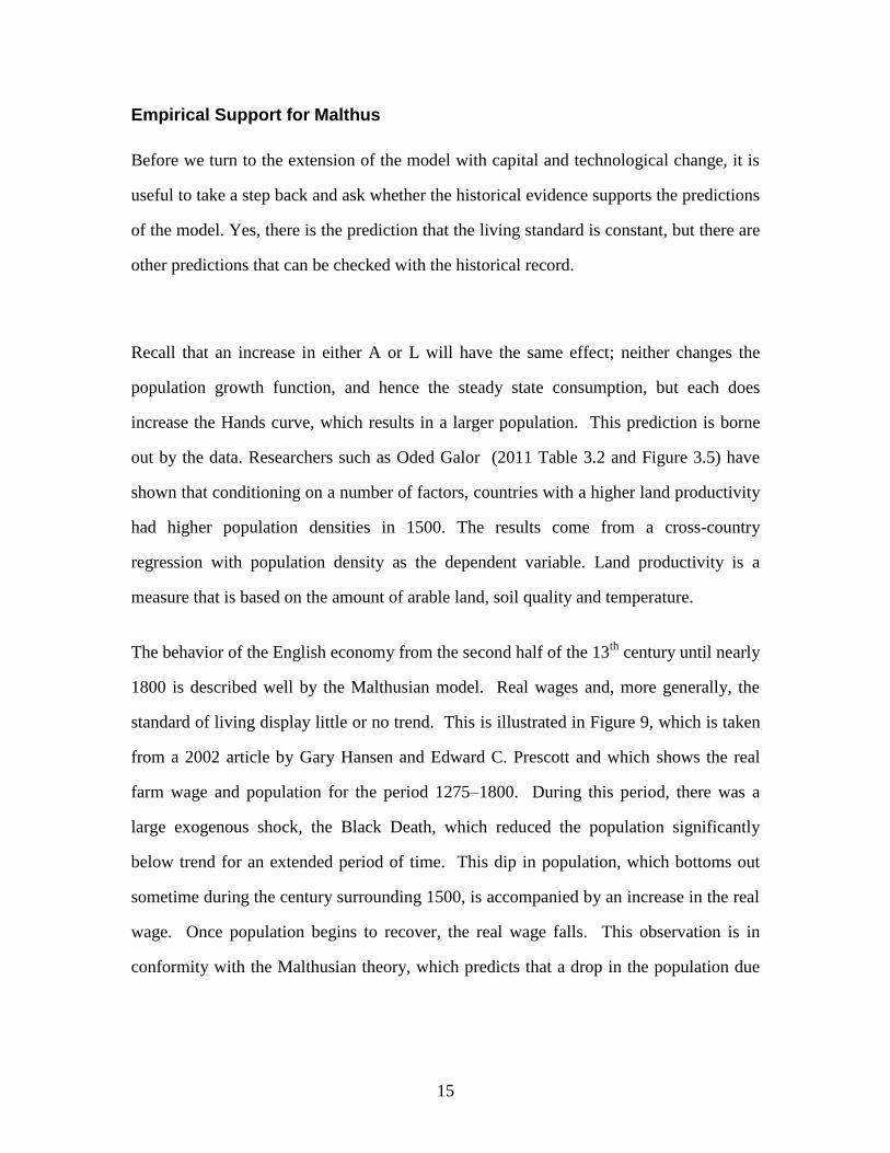
standard of living display little or no trend. This is illustrated in Figure 9, which is taken

from a 2002 article by Gary Hansen and Edward C. Prescott and which shows the real

farm wage and population for the period 1275–1800. During this period, there was a

large exogenous shock, the Black Death, which reduced the population significantly

below trend for an extended period of time. This dip in population, which bottoms out

sometime during the century surrounding 1500, is accompanied by an increase in the real

wage. Once population begins to recover, the real wage falls. This observation is in

conformity with the Malthusian theory, which predicts that a drop in the population due

16

to factors such as plague will result in a high labor marginal product, and therefore real

wage, until the population recovers.

Figure 9

0

50

100

150

200

250

300

1275 1350 1425 1500 1575 1650 1725 1800

Population and Real Farm Wage

Population

Wage

Source: Hansen and Prescott 2002

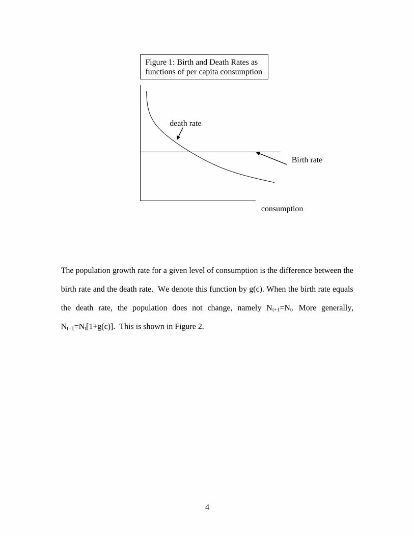
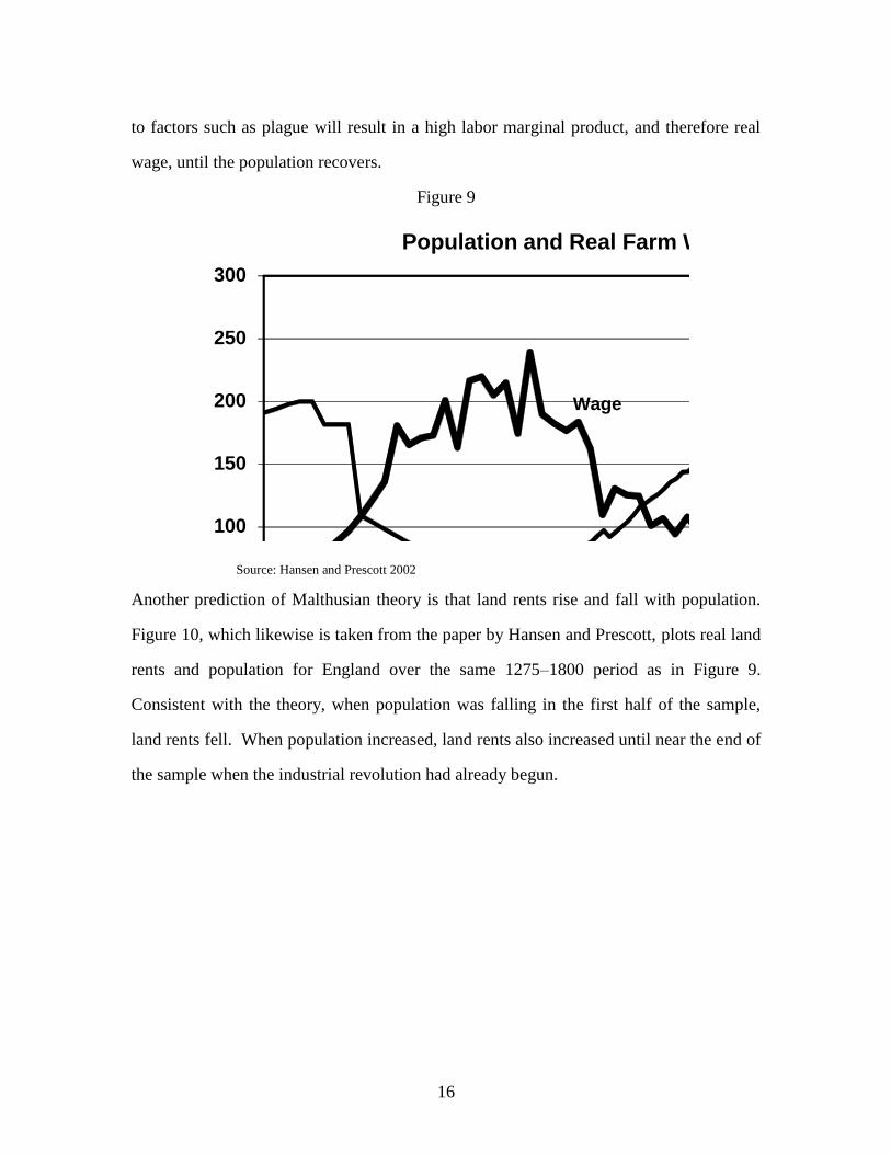
Another prediction of Malthusian theory is that land rents rise and fall with population.

Figure 10, which likewise is taken from the paper by Hansen and Prescott, plots real land

rents and population for England over the same 1275–1800 period as in Figure 9.

Consistent with the theory, when population was falling in the first half of the sample,

land rents fell. When population increased, land rents also increased until near the end of

the sample when the industrial revolution had already begun.

17

Figure 10

0

50

100

150

200

250

300

1275 1350 1425 1500 1575 1650 1725 1800

Population and Real Land Rent

Population

Rent

III. Technological Change and Capital

Thus far we have shown that the steady state of the Malthusian

model without technological change and capital is characterized by

a constant living standard and zero population growth. Recall, that

we are after a model of the pre-1700 era that generates a constant

living standard and population growth. The simple Malthus model

fails to deliver sustained increases in an economy’s population. We

now add capital and technological change with the intent of seeing

if these additions change the model’s predictions. With the

addition of capital it is no longer possible to characterize the

properties of the model graphically. For this reason we will proceed

When Bad Hygiene is Good- A Farewell to Alms.

Gregory Clark, an innovative economic historian at the University of California at Davis, compare England and Japan through the lens of the Malthus Model in order to understand why England was the first nation to industrialize. Although we postpone a discussion of the industrial Revolution to the next chapter, it is useful to consider Clark’s hypothesis in the context of our study of the Malthus model. Clark documents in his book A Farewell to Alms: A Brief Economic History of the World, that when it came to personal hygiene, the British were notoriously bad. The Japanese, in contrast, were remarkably advanced in their hygiene. Clark documents that well organized market for human feces used as fertilizer in agricultural production. In the context of the Malthus Model, the lack of hygiene in England implied a higher death rate, and a higher living standard. The Japanese, although cleaner and with a lower death rate, had a lower living standard.

18

by deriving algebraically the steady state of the model.

It is possible to give some intuition for the algebraic results that will be derived, however.

First, let us think back to the Solow model without technological change. Was there

sustained growth in the per capita consumption and output in that model without

technological change? The answer we found was No! More specifically, we showed that

sustained growth was not possible on account of the law of diminishing returns. In the

Malthus model the law of diminishing returns still holds so adding capital to the Malthus

model will do nothing to change the result of a constant living standard. How about the

affect of adding capital accumulation on population growth: will it change the result of

zero population growth in the steady state? Again, it will not; you could double all the

people and machines and output would less than double because land is fixed. Here we

see the importance of the fixed factor property of land. Then why are we adding capital

to the model? As mentioned at the beginning of the Chapter, capital is added with future

work in mind. In two chapters we will combine the Malthus model with the Solow

model. As capital accumulation is a fundamental component of the Solow model, we add

it to the Solow model to have a unified and harmonious structure.

What are the implications of adding technological change? To gain some intuition here,

it is useful to revisit the comparative static analysis of the Malthus model without

technological change or capital accumulation. Recall, a higher land quality or TFP is

associated with a larger steady state population but no change in the living standard. If

we take this a step further, and envision TFP increasing every period by the same factor,

then the implication is that we will have a steady state with constant population growth

and a constant living standard- the pre-1700 facts. This is what we now show.

19

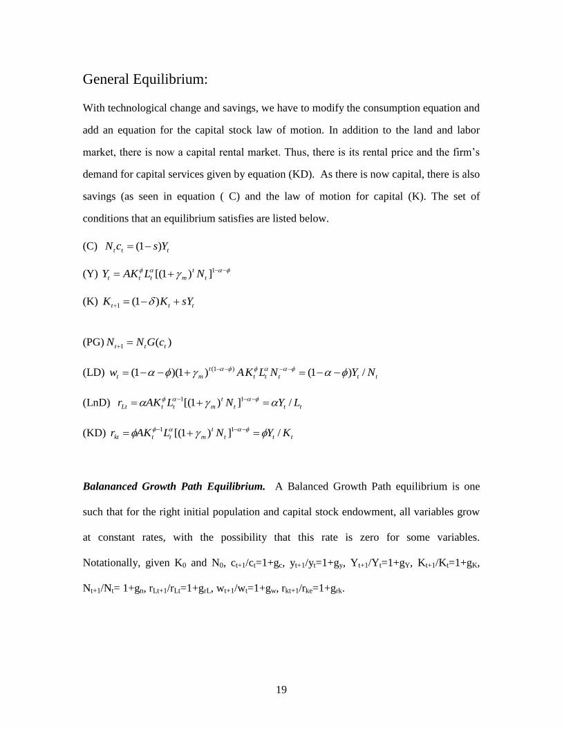
General Equilibrium:

With technological change and savings, we have to modify the consumption equation and

add an equation for the capital stock law of motion. In addition to the land and labor

market, there is now a capital rental market. Thus, there is its rental price and the firm’s

demand for capital services given by equation (KD). As there is now capital, there is also

savings (as seen in equation ( C) and the law of motion for capital (K). The set of

conditions that an equilibrium satisfies are listed below.

(C) ttt YscN )1(

(Y) 1])1[( t

t

mttt NLKAY

(K) ttt sYKK )1(1

(PG) )(1 ttt cGNN

(LD) ttttt

t

mt NYNLKAw /)1()1)(1( )1(

(LnD) ttt

t

mttLt LYNLKAr /])1[( 11

(KD) ttt

t

mttkt KYNLKAr /])1[( 11

Balananced Growth Path Equilibrium. A Balanced Growth Path equilibrium is one

such that for the right initial population and capital stock endowment, all variables grow

at constant rates, with the possibility that this rate is zero for some variables.

Notationally, given K0 and N0, ct+1/ct=1+gc, yt+1/yt=1+gy, Yt+1/Yt=1+gY, Kt+1/Kt=1+gK,

Nt+1/Nt= 1+gn, rLt+1/rLt=1+grL, wt+1/wt=1+gw, rkt+1/rke=1+grk.

20

We solve for the balanced growth path equilibrium in two parts. In the first, we derive the

growth rates of each of the key variables along the balanced growth path. This is Part I.

In the second part, we solve for the paths or levels of the population and the total capital

stock, as well as their initial values.

Part 1. Solving for the growth rates along the balanced growth path.

Step 1. Use equation (PG) and invoke the BPG condition that Nt+1/Nt= 1+gn . From this

we conclude that gc= 0 and ct=css

.

Step 2: Use equation (C) and use the result that gc= 0 to conclude that gn=gY.

Step 3. Use equation (K) to conclude that gK=gY. To do this, first divide both sides by Kt.

This is

tttt KsYKK /)1(/1 .

Next invoke the BGP condition that Kt+1/Kt=1+gK. This is

t

tK

K

Ysg )1(1

As the left hand side of the equation is constant, it follows that Y and K must grow at the

same rate along the balanced growth path.

Step 4. We now use the above results, that gK= gn = gY ≡ g with equation (Y) to solve for

g. First take the date t+1 output. This is

1

1

1

111 ])1[( t

t

mttt NLKAY

Next take the date t+1 output as a ratio of the date t output. This is

1

1

1

1

111

])1[(

])1[(

t

t

mtt

t

t

mtt

t

t

NLAK

NLAK

Y

Y

21

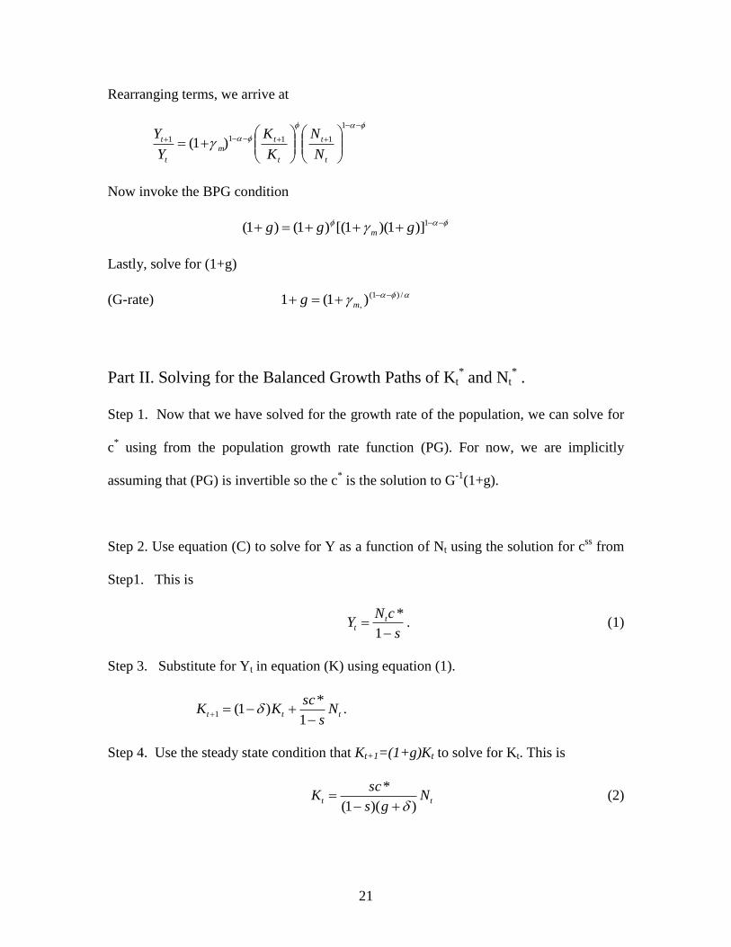
Rearranging terms, we arrive at

1

1111 )1(t

t

t

tm

t

t

N

N

K

K

Y

Y

Now invoke the BPG condition

1)]1)(1[()1()1( ggg m

Lastly, solve for (1+g)

(G-rate) /)1(

, )1(1 mg

Part II. Solving for the Balanced Growth Paths of Kt* and Nt

* .

Step 1. Now that we have solved for the growth rate of the population, we can solve for

c* using from the population growth rate function (PG). For now, we are implicitly

assuming that (PG) is invertible so the c* is the solution to G

-1(1+g).

Step 2. Use equation (C) to solve for Y as a function of Nt using the solution for css

from

Step1. This is

s

cNY t

t

1

*. (1)

Step 3. Substitute for Yt in equation (K) using equation (1).

ttt Ns

scKK

1

*)1(1 .

Step 4. Use the steady state condition that Kt+1=(1+g)Kt to solve for Kt. This is

tt Ngs

scK

))(1(

*

(2)

22

Notice that equation (2) gives us the steady state per capita capital stock if we divide both

sides by Nt.

Step 5. Next take equation (Y) substituting for Yt into equation (K). This is

1

1 ])1[()1( t

t

mtttt NLKsAKK . (3)

Step 6: We again invoke the steady state condition Kt+1=(1+g)Kt and use equations (2)

and (3) to arrive at

11

1

])1[())(1(

*)( t

t

mtt NLNgs

scsAg

This gives us a single equation in a single unkown, Nt. Solving for Nt yields

(N-SS)

/11

/)1(*

))(1(

*)1(

gs

sc

g

sALN t

mt

Using equation (N-SS) with (2), gives us the solution for *

tK

Computing the Equilibrium path when *

00 NN or *

00 KK .

If *

00 NN or *

00 KK , the economy will not be on its balanced growth path. We

showed graphically for the Malthusian model without capital accumulation and

technological change that an economy which does not begin on its steady will converge

to it. Although we cannot show it graphically for this more complex version of the

model, the convergence result holds.

23

It is easy to compute the transitional path for the model economy via a spreadsheet once

we assign parameter values to the model. The algorithm for computing the equilibrium

path is straightforward. The equilibrium consists of a path for the following set of

variables: ),,,,,,,( KtLttttttt rrwKLYNc . The equilibrium quantities are trivial to find

because the supply of land, labor and capital are all vertical. That is to say in period t, the

amount of capital used is Kt; the amount of labor used is the population, Nt; and the

amount of land used is just the endowment L. We therefore can determine output Yt and

ct. We also know what the marginal products of all the inputs are, so we know all of the

prices. We can then figure out next period’s population and capital stock using the

population growth rate function, G(ct) and the capital stock law of motion.

The period t=0 quantities of land, capital and people are given. Once you have these

initial conditions, the entire path can be determined robotically. More specifically, we

compute the equilibrium path as follows: Given land, L , K0, and an initial population N0,

we find the equilibrium path in each period as follows:

1. Determine Yt from the aggregate production function, Equation(Y).

2. Determine ct from (C)

3. Determine Kt+1 from (K) using Yt

4. Determine Nt+1 from (PG) using ct.

5. Go back to Step 1 and Repeat.

24

IV. Calibration to pre-1700 Observations

We now calibrate the model. We do not do so in the context of the five step process,

where we start with a particular question in mind. For instance, we could ask the

question of whether differences in land quality can account for differences in population

densities in the pre-modern era. Instead, we essentially consider Steps 3 and Step 4 in the

calibration, with a particular emphasis on the parameters associated with the production

function and the population growth rate function. We do this with an eye to calibrating

the combined model. This is why we do not go through the five calibration steps.

The assignment of parameters is done so that the balanced growth path matches the pre-

1700 growth facts. The parameters for which we need to assign values are:

Asm ,,,,, . In addition we need to specify the population growth function and

assign parameter values to that function.

In what follows, we assign parameter values associated with the production function so

that the model matches the following pre-1700 observations associated with England’s

experience. As reported by Hansen and Prescott (2002), the key pre-1700 observations

are:

1. an average annual population growth rate of .003 per year.

2. Historians’ estimates of labor’s share of income equal to 2/3.

3. Historians’ estimates of Land’s share of income at 3/12.

4. Historians’ estimates of capital’s share of income at 1/12.

25

We continue to set the savings rates, s= .20 that we used for the Solow model.

Additionally, we continue to use the depreciation rate that we used for the Solow model,

namely, δ = .05. The savings rate for pre-1700 England was surely lower than 20

percent. The reasons that we keep these parameter values at the Solow calibrated values

are twofold. First, two chapters from now we will study a combined Malthus and Solow

model. Thus, it is convenient to keep these parameter values the same in this combined

model. Second, savings rates probably did not differ so much across countries before

1700 and so what its value was before 1700 is not quantitatively important in

understanding differences in starting dates across countries.

Just as in the Solow model, an input’s share of income equals its coefficient in the

production function. For land, this coefficient is α; for capital, this coefficient is ; and

for labor this coefficient is just 1 . Thus, consistent with the historical record, we

set 12/3 and 12/1 . We can determine the growth rate of technological change,

γm using the balanced growth relation between population growth and the exogenous

growth rate of technological change. This is

/)1(

, )1(1 mg .

Using the observation that g=.003 and the values for 12/3 and 12/1 , we can

solve for the value of γm. This is 001.m . The parameterized production function is

thus

3/212/312/1 ])001.1[( t

t

tt NLAKY .

Just as in Solow, we are free to choose the units in which we measure output. In Solow,

we did this in the context of normalizing the TFP parameter to one. Here we do a similar

26

normalization, except that we normalize the TFP parameter and land L to one in the

production function. This we can do because land, being fixed and TFP in the production

function A, have the same effect on output. That is to say for any amount of land, L, we

could always adjust A so that the term ALα is the same number.

The Population growth function

For the predictions of Malthus to hold, we need a population growth function that is

increasing in consumption. As the model predicts a constant population growth along the

balanced growth path, it is clear that we need an episode where the English economy was

not on its balanced growth path in order to estimate the growth rate function. Looking at

the historical picture, the English economy appears to be off its balanced growth path

much of the 1300-1600 period on account of the Black Death, which started between

1347 and 1350. The effect of the Black Death on Europe’s population was dramatic;

historians estimate that one half to one third of Europe’s population died in this three year

period, and it took nearly 200 years for the population to return to its pre 1346 level in

Europe.

Although the English economy was not on its balanced growth pathe during the 14th

century, using this period to estimate the growth rate function is problematic in that the

death rate clearly was changing. This implies that the population growth rate function

was shifting over this period. For this reason, we look for a sub-period over the 1400-

1650 period for which the relation between the living standard and the population growth

27

rate for England appears to stable in the sense of no shifts in the population growth rate

function. A period for which this appears to be the case is the 1500-1560 period.

Although the model assumes that the population growth rate is a function of consumption

per capita, we estimate it using real income, (actually real wages) for England instead.

The reason for doing so is consumption data in this period is hard to find. As savings

were not high back then, there is little difference in using income instead of consumption

to estimate the population growth function.

The population data and real GDP per capita data are based on Clark (2009, Tables 7 and

28). We simply use the data to estimate the following

ttt cNN ln/ 101 .

β0 is the y-intercept of this log-linear relation and β1 is the slope. The choice of the log of

consumption as the independent variable instead of consumption is used as the raw data

suggests such a logarithmic relation rather than linear.

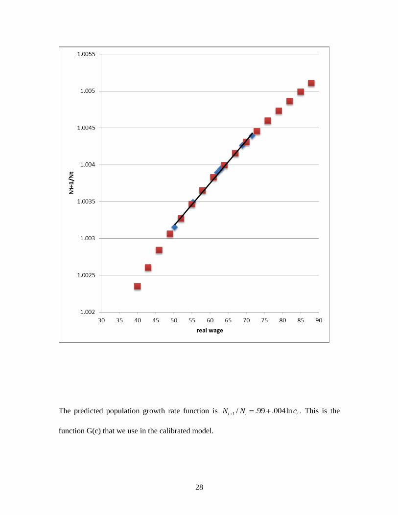
The actual and predicted population growth rates for the England are shown in the

following figure. The horizontal axis is English real wages.

28

The predicted population growth rate function is ttt cNN ln004.99./1 . This is the

function G(c) that we use in the calibrated model.

29

V. Conclusion

The Malthusian model has a long tradition in economics being developed by the Classical

Economists. It was put forward to capture the pattern of development before 1700,

namely, a constant living standard and positive population growth. These results follow

from two key features of the model: a population growth rate function that increases in

consumption and a constant returns production function with a fixed factor.

Although a good representation of history up to 1700, the Malthus model is not useful for

understanding the modern growth era. Nevertheless, we shall see that if it is combined

with the Solow growth model, we have a model that captures the essential growth and

development facts. This is a key objective in the chapters to come.

References

Clark, Gregory 2009. "The Macroeconomic Aggregates for England, 1209-2008,"

Working Papers 919, University of California, Davis, Department of Economics.

Galor, Oded. 2011 Unified Growth Theory. Oxford University Press: Oxford and

Princeton

Hansen, Gary and Edward C. Prescott. 2002. “Malthus to Solow”. AER Papers and

Proceedings. 92: 1205-1217.

Mokyr, Joel (1990). The Lever of Riches: Technological Creativity and Economic

Progress. Oxford: Oxford University Press.

30

Problems:

Questions 1-4 use the simplest version of the Malthusian model with just land and labor

inputs.

1. What effect would a decrease in TFP have on the equilibrium standard of living,

and population, both in the short-run and the long-run?

2. What does the Malthus model predict for short-run and long-run output and

population differences between countries that differ in geography? (Say one

country has infertile land.)

3. How do the short-run predictions of the model change if the birth rate was an

increasing function of the level of consumption?

4. Between 1400 and 1700, women in England started to marry later in life. Show

how this change would impact the standard of living both in the short run or long

run.

5. This question 5 pertains to the Malthusian Model with both exogenous technological

change and capital accumulation. Show either mathematically or graphically, how the

rental price of capital, the rental price of land, and the real wage change in the long-run.

6. Malthus Excel Exercise- For this problem you will need to use an excel spreadsheet.

Variable Meaning / Value

Ct Aggregate consumption of food

ct Individual consumption of food

Nt Number of people

Lt Acres of land (fixed amount) =

10,000,000,000

Kt Aggregate capital Stock

31

Yt Total Output

Nt Total population

Endowments: People own the economy’s stock of land and its capital. Each person

also has one unit of time for which he can supply to the labor market.

Preferences

People save a fixed fraction s=.20 of their income.

The production function is 3/212/312/1 ])001.1[( t

t

ttt NLAKY .

Capital Stock law of motion

ttt YKK 2.95.1

The Population growth function

ttt cNN ln004.99./1 . This is the function G(c).

Q1. Balanced growth Path Results

a. Solve for the balanced growth path level of c.

b. Solve for the Balanced Growth path population at time t=0, N0.

c. Solve for the Balanced Growth path aggregate capital stock at date t=0, K0.

Q.2 Transitional Dynamics

a. Suppose that the economy is on its balanced growth path from t=0, 49. Then at

t=50, there is an epidemic that kills off 1/3 of the date t=49 population. (Thus,

N50=2/3 N49.) Calculate the paths for Nt, ct, and Kt from t=50 to 250. Produce a

time plot graph for the log of each variable. Does the system converge to the

balanced growth path solution?

b. Suppose that the economy is on its balanced growth path from t=0, 49. Then at

t=50, there is an event that increases the birth rate, the effect of which is to raise

32

the intercept of the population growth function to 1.5. Calculate the paths for Nt,

ct, and Kt from t=50 to 150. Produce a time plot graph for the log of each

variable. Does the system converge to the balanced growth path solution?