The long-wave instability of short-crested waves, via embedding in the oblique two-wave interaction

J. Fluid Mech. (2005), vol. 543, pp. 147–182. c© 2005 Cambridge University Press

doi:10.1017/S0022112005006270 Printed in the United Kingdom

147

The long-wave instability of short-crestedwaves, via embedding in the oblique

two-wave interaction

By THOMAS J. BRIDGES AND FIONA E. LAINE-PEARSONDepartment of Mathematics and Statistics, University of Surrey, Guildford, Surrey, GU2 7XH, UK

(Received 10 October 2003 and in revised form 7 January 2005)

The motivation for this work is the stability problem for short-crested Stokes waves.A new point of view is proposed, based on the observation that an understandingof the linear stability of short-crested waves (SCWs) is closely associated with anunderstanding of the stability of the oblique non-resonant interaction between twowaves. The proposed approach is to embed the SCWs in a six-parameter family ofoblique non-resonant interactions. A variational framework is developed for theexistence and stability of this general two-wave interaction. It is argued that theresonant SCW limit makes sense a posteriori, and leads to a new stability theory forboth weakly nonlinear and finite-amplitude SCWs. Even in the weakly nonlinear casethe results are new: transverse weakly nonlinear long-wave instability is independentof the nonlinear frequency correction for SCWs whereas longitudinal instability isinfluenced by the SCW frequency correction, and, in parameter regions of physicalinterest there may be more than one unstable mode. With explicit results, a critique ofexisting results in the literature can be given, and several errors and misconceptionsin previous work are pointed out. The theory is developed in some generality forHamiltonian PDEs. Water waves and a nonlinear wave equation in two spacedimensions are used for illustration of the theory.

1. IntroductionThe aim of this paper is to develop a theory for the long-wave instability of short-

crested Stokes waves (SCWs). These waves are one of the simplest classes of doublyperiodic three-dimensional water waves and are therefore of fundamental interest,and they are of practical importance since they appear in models for coastal sandtransport, reflection off vertical seawalls, and wave propagation along channels.

Historically, the problem of stability of SCWs has been approached directly. Roskes(1976b) proposed the use of coupled nonlinear Stokes (NLS) equations to model SCWinstability, Mollo-Christensen (1981) proposed the use of Whitham modulation theory,Ioualalen & Kharif (1994) computed eigenvalues of the exact linear stability problemnumerically, and Badulin et al. (1995) presented a qualitative analysis based on theZakharov (1968) Hamiltonian formulation for water waves. As far as we are awarethese are the only papers in the literature on a theoretical approach to the linearstability of SCWs.

However, Roberts (1983) points out that SCWs are a special case of two-phasewavetrains, and he proposes that the theory of Ablowitz & Benney (1970), wheremodulation equations for multi-phase wavetrains are derived, be used for the stability

148 T. J. Bridges and F. E. Laine-Pearson

(k1, l1)

(k2, l2)

k

l(k, l)

(k, – l)

Figure 1. Schematic of the deformation of an SCW into a two-wave interaction.

analysis. It is possible that this approach would work, but the Ablowitz–Benneyequation is non-local and not easy to work with. However, embedding the SCWs ina two-phase wavetrain turns out to be the correct approach.

The basic observation is that an understanding of the linear stability of SCWs – evenweakly nonlinear SCWs – is closely associated with understanding the stability of theoblique non-resonant interaction between two waves. One way to see the connectionbetween SCWs and two-wave interaction is to note that when an SCW becomesunstable to long-wave perturbations, the resonant SCW plus the perturbation is awave with a wavenumber vector which is no longer resonant.

This observation is a generalization to two space dimensions of the geometry ofsideband instability. A weakly nonlinear Stokes wave is stable to perturbations of thesame wavelength. However, if a perturbation of a slightly longer wavelength is added,it is unstable. This instability is determined by the susceptibility of the Stokes wave towaves with slightly longer wavelength. In the case of SCWs there are two sidebands:sidebands in wavenumber space associated with both the x and y directions. Thereforethe perturbed wavenumber vector is perturbed in both length and direction.

In the theory proposed here, the SCW is first embedded in a six-parameter familyof multi-phase wavetrains, as shown schematically in figure 1, and then a posteriorithe limit to resonant SCWs is taken, accumulating along the way enough informationto predict all the long-wave instabilities of SCWs. Effectively, the embedding providesinformation about the susceptibility of the SCW to distortion in wavenumber spaceby the perturbation.

A by-product of this analysis is a stability theory for the general two-phase wave-train, which may be of independent interest. For example Onorato et al. (2003) showthat the instability of the non-resonant two-wave interaction may explain the double-peaked power spectrum of waves in shallow water observed by Smith & Vincent(1992).

The existence of the SCWs is assumed throughout, and attention is restricted togravity waves on a fluid of infinite depth, although the implications for other classesof waves will be apparent. There is now a range of analytical and numerical existenceresults in the literature that we can appeal to (e.g. Hsu, Silvester & Tsuchiya 1980;Roberts 1983; Roberts & Peregrine 1983; Ioualalen 1993; Kimmoun, Branger &Kharif 1999; Craig & Nicholls 2000, 2002 and references therein). A rigorous theoryfor the existence of gravity SCWs has been elusive and Craig & Nicholls (2002) pointout that there are technical problems associated with small divisors. However, in thecase of capillary–gravity SCWs there is a well-developed existence theory (Craig &Nicholls 2000).

Instability of short-crested Stokes waves 149

In addition to the existence of SCWs, the theory also uses an embedding of SCWsin a general non-resonant two-phase wavetrain. Historically, the analyses of two-wave and n-wave interactions have been considered independently of SCWs. Theonly results in the literature for the general two-wave interaction are for the weaklynonlinear case (e.g. Longuet-Higgins 1962; Willebrand 1975; Weber & Barrick 1977;Pierson 1993; Elfouhaily et al. 2000 and references therein). It is easy to show thatapplying the SCW limit to the (weakly nonlinear) two-wave interaction results in theusual (weakly nonlinear) SCW solutions. However, a key new feature of the theoryhere is that information is extracted from the embedding, before the limit to SCWs istaken.

In this paper, a theory for the stability of weakly nonlinear SCWs and finite-amplitude SCWs is developed. The only restriction is on the perturbation wave-numbers, which are restricted to long-wave perturbations. These perturbations aregeneralizations of the Benjamin–Feir instability of plane travelling waves.

A Stokes-type expansion for SCWs is singular in the long-crested limit (seeRoberts & Peregrine 1983, where an alternative theory is proposed which avoidsthe singularity). Since this paper is primarily concerned with periodic SCWs, it isassumed throughout that the parameter values for the SCWs are chosen away fromthe long-crested limit. Since the waves under consideration in this paper are in infinitedepth, mean flow will be ignored. It is important to note that neglect of mean flow isan assumption. It is certainly true for weakly nonlinear SCWs in infinite depth, but itis an open question whether wave-generated mean flow can occur for finite-amplitudeSCWs. The formulation presented here is amenable to including mean flow effects(see discussion in § 10). However, it is assumed in this paper that the SCWs are notaccompanied by wave-generated mean flow.

The water-wave problem is Hamiltonian, and it will be advantageous to recognizethis in the development of the theory. The Hamiltonian approach was first applied byBadulin et al. (1995) to the analysis of SCWs and it was shown to have advantages.This idea is taken a step further here with the use of the multi-symplectic formulationof Hamiltonian PDEs. Since water waves and other Hamiltonian PDEs for SCWscan be reformulated as multi-symplectic systems, a general formulation of multi-symplectic Hamiltonian PDEs can be taken as the starting point

MZt + KZx + LZy = ∇S(Z), Z ∈ , (1.1)

where M, K and L are constant skew-symmetric operators, is a linear space (eithern for the nonlinear wave equation or an inner-product space of functions on thecross-section for water waves), and the gradient of S is with respect to the innerproduct on . Details of this formulation for water waves and other HamiltonianPDEs can be found in Bridges (1996, 1997a, b) and the details needed here arerecorded in § 2, including a new multi-symplectic formulation of the nonlinear waveequation in two space dimensions. This nonlinear wave equation provides a simplemodel problem for SCWs and an example where the long-wave transverse instabilityof SCWs can disappear at low amplitude.

The advantage of the multi-symplectic framework is five-fold: (a) it is clear andunambiguous how to formulate the long-wave stability theory, using only the structureof the equations; (b) embedding the stability problem in the two-wave interaction is anatural part of the multi-symplectic approach and provides further information aboutthe nature of the instability; (c) explicit results for weakly nonlinear water waves canbe obtained; (d ) general conclusions about SCW instability for other systems are alsodeduced; (e) it is straightforward to include meanflow effects.


What is a SCW? The definition is implicit in the literature, and in Appendix A anexplicit definition of SCWs is given. A solution, say Z(x, y, t) of (1.1), is called an SCWif it is periodic in x, y and t , travelling in the x-direction (a function of x and t in linearcombination only), and is invariant under reversibility in the y-direction. A definitionof y-reversibility with examples is given in § 2. An immediate and illuminatingconsequence of this definition is that SCWs have zero transverse momentum –but certainly have non-zero longitudinal momentum. This property of SCWs is usefulfor interpreting the embedding of SCWs in a two-phase wavetrain: the embeddingdeforms the SCWs into waves with non-zero transverse momentum, thereby testingthe susceptibility of SCWs to perturbation of the transverse momentum.

Much of the paper is devoted to the existence, properties and stability of the obliquetwo-wave interaction. Let η(x, y, t) represent the free-surface elevation. The obliquetwo-wave interaction of water waves is a solution of the form

η(x, y, t) = η(θ1, θ2), (1.2)

where

θj = kjx + jy + ωj t + θ0j (j = 1, 2), (1.3)

and (kj , j ) are the wavenumbers, ωj are the frequencies, θ0j are phases, and η is a 2π

periodic function of θ1 and θ2. A short-crested wave is the special case: k2 = k1 = k,2 = −1 = − and ω2 = ω1 = −ω, and it is reversible in the y-direction (invariant underchange of sign of y; precise definition given in § 3 and Appendix A). In the linearand weakly nonlinear limit this latter condition reduces to the familiar requirementof equal amplitudes of the two component waves.

The strategy is to construct variational principles for the general two-wave interac-tion. The variational principles provide natural Jacobians which contain informationabout the susceptibility of the SCW to distortion into oblique non-resonant two-waveinteraction.

The linear stability problem for the general two-wave interaction is then formulatedand a stability condition derived. Long-wave perturbations are of the form

η(x, y, t) = η(θ1, θ2) + Re(N(θ1, θ2)e

i(αx+βy+Ωt))

with |α|, |β| 1.

The basic state is unstable when Im(Ω) < 0. This condition can be strengthened toIm(Ω) = 0 by noting that the Hamiltonian symmetry assures us that there exists aneigenvalue with Im(Ω) < 0 whenever one exists with Im(Ω) > 0.

The main result is that all long-wave instabilities (of SCWs or the two-waveinteraction) are predicted by the zeros of the quartic polynomial

(Ω, α, β) = det[N2Ω2 + N1Ω + N0] (1.4)

where Nj are 2×2 matrices dependent on α, β and the basic state. Precise expressionsfor these matrices are given in § 5. Taking the limit to SCWs in the matrices Nj leadsto a linear stability quartic for SCWs. Details of the results for SCWs are given in§ § 6 and 7.

The general result (i.e. not just for water waves) for the weakly nonlinear case canbe summarized as follows. Let D(ω, k, ) be the dispersion relation for the linearproblem, and suppose parameter values are chosen so that

Dω = 0, Dk = 0, D = 0.

Consider a weakly nonlinear solution of (1.1) of the form

Z(x, y, t) = Z(x, y, t) = A1 ξ ei(kx+y−ωt) + A2 ξ ei(kx−y−ωt) + c.c. + · · · , (1.5)


where ξ is an eigenvector determined by the linearized operator, A1 and A2 arecomplex amplitudes and the higher-order terms are higher order in |A1| and |A2|. Toleading order, the complex amplitudes satisfy

0 = A1(D(ω, k, ) + a|A1|2 + b|A2|2 + · · ·),0 = A2(D(ω, k, ) + b|A1|2 + a|A2|2 + · · ·),

(1.6)

where a and b are the coefficients for the nonlinear correction terms of the dispersionrelation.

Clearly when |A2| = 0 and |A1| =0 (or vice versa) the basic state is a travelling wavewith frequency change

ω = ω0 + ωTW2 |A1|2 + · · · where ωTW

2 = − a

Dω

, (1.7)

where D(ω0, k, ) = 0 and Dω is evaluated at ω = ω0. On the other hand, SCWs satisfy|A1| = |A2| and so their frequency change is

ω = ω0 + ωSCW2 |A1|2 + · · · where ωSCW

2 = − (a + b)

Dω

. (1.8)

Now, add a long-wave perturbation to (1.5)

Z(x, y, t) = Z(x, y, t) + Re(Ξ ei(αx+βy+Ωt)

)with |α|, |β| 1. (1.9)

For the linearization about weakly nonlinear SCWs, the stability quartic (1.4) forperturbations (1.9) has an interesting factorization into four branches (noting that|A1| = |A2| := |A| for these waves)

Ω =

−Dkα − Dβ

Dω

− σ+ |A| + · · · ,

−Dkα − Dβ

Dω

+ σ+ |A| + · · · ,

−Dkα + Dβ

Dω

− σ− |A| + · · · ,

−Dkα + Dβ

Dω

+ σ− |A| + · · · ,

(1.10)

when β = 0 (transverse instability) with

σ 2+ = (ωkkα

2 + 2ωkαβ + ωβ2)ωTW

2 ,

σ 2− = (ωkkα

2 − 2ωkαβ + ωβ2)ωTW

2 .

(1.11)

The derivatives of ω(k, ) are obtained by differentiating D(ω(k, ), k, ) = 0. Notethat it is the TW correction and not the SCW correction to the frequency whichappears at leading order in the stability exponents for transverse instability.


(a) (b)

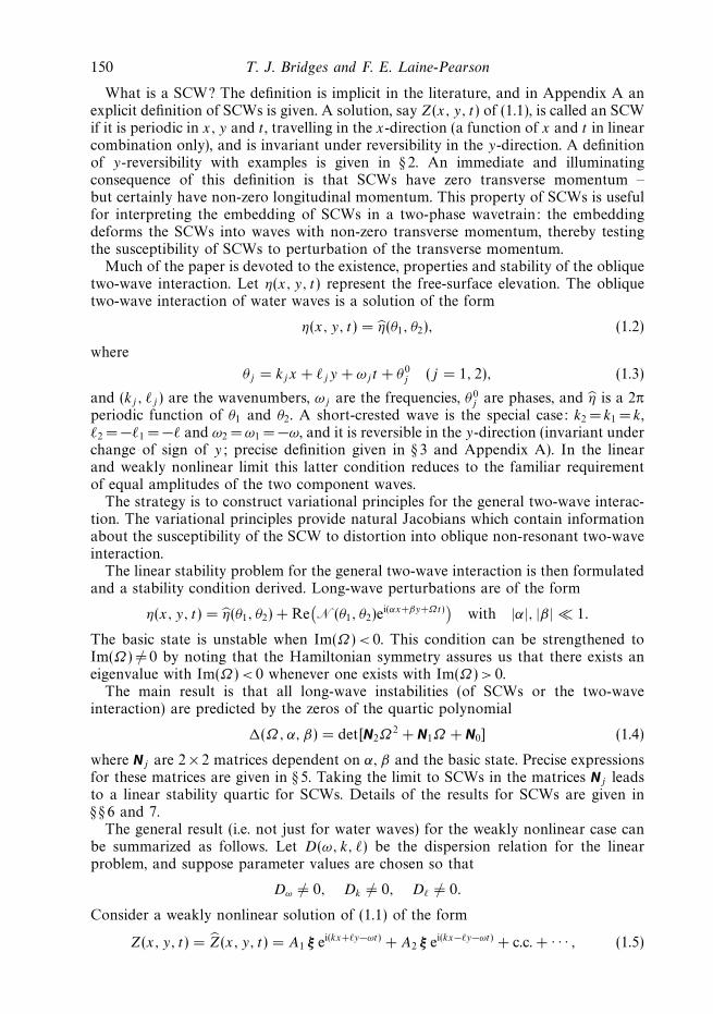
Figure 2. A schematic showing the typical qualitative position of the eigenvalues λ= ±iΩfor (1.10) when (a) |A| = 0 and (b) |A| > 0.

When β =0 (longitudinal instability), the factorization changes to

Ω =

− Dk

Dω

α − µ+ |A| + · · · ,

− Dk

Dω

α + µ+ |A| + · · · ,

− Dk

Dω

α − µ− |A| + · · · ,

− Dk

Dω

α + µ− |A| + · · · ,

(1.12)

with

µ2+ = ωkkω

SCW2 α2,

µ2− = ωkk

(2ωTW

2 − ωSCW2

)α2.

(1.13)

A weakly nonlinear SCW is unstable if any of the four quantities σ 2+, σ 2

−, µ2+ or µ2

−is negative.

Throughout it is assumed that σ+, σ−, µ+ and µ− are non-vanishing and of orderone. There are lines in perturbation wavenumber space, and particular values of thewavenumber vector of the SCWs, where these coefficients vanish. Equation (1.19)shows an example of these resonance lines, and further discussion is given in § 7.When one of these coefficients vanishes, the weakly nonlinear stability properties aredetermined at the next order in |A|.

The stability exponents are λ= ± iΩ with Ω given by (1.10) or (1.12). When |A| = 0and β = 0 there is a double resonance, as shown schematically in figure 2(b), plottedin the complex λ-plane. The precise position of the resonances depends on the valuesof (k, ) and (α, β). For β = 0, both pairs coalesce and the resonance is fourfold. When|A| > 0 the resonances split, and may become unstable. The most dramatic situationwhere β = 0 and two modes become unstable is shown in figure 2(b).

The information contained in (1.10) and (1.12) can be summarized as follows. LetD(ω, k, ) be the dispersion relation of the linearized problem and let (ω, k, ) bethe frequency and wavenumbers of the weakly nonlinear SCW (or to leading orderthe values for the linearized problem). Then there are two alternatives for instability


when β = 0. First, if Dω = 0 and

det

Dωω Dωk Dω Dω

Dkω Dkk Dk Dk

Dω Dk D D

Dω Dk D 0

> 0, (1.14)

the weakly nonlinear SCW is unstable. Secondly, if the determinant (1.14) is negativebut

ωkk ωTW2 < 0, (1.15)

the basic SCW is unstable, where ωTW2 is the frequency correction in (1.7), and ωkk is

the second derivative of ω associated with the x-direction only.Longitudinal instabilities (β = 0) are determined by the signs of µ2

± in (1.13). Thefirst condition,

ωkkωSCW2 < 0,

is similar to the condition proposed by Molloo-Christensen (1981), although ωkk heredepends on whereas in Mollo-Christensen (1981) the -dependence is neglected (seediscussion below). The second condition is

ωkk

(2ωTW

2 − ωSCW2

)< 0.

This condition is related to the condition proposed by Roskes (1976b). Clearly asufficient condition for longitudinal instability is µ2

+µ2− < 0 which results in

0 > µ2+µ2

− = ω2kkα

4ωSCW2

(2ωTW

2 − ωSCW2

)=

ω2kk

D2ω

α4(a2 − b2) (1.16)

or |b| > |a| which is precisely the condition proposed by Roskes (1976b). However, thisis only a sufficient condition. It misses the case where both µ2

− and µ2+ are negative,

which occurs for water waves.The condition (1.14) is a sufficient condition for the right-hand side in (1.11) to

be factorizable with real factors. When σ 2+ is factorizable, there is always a wedge

emanating from the origin in the (α, β)-plane where at least one of the roots of (1.10)is unstable. The determinant condition (1.14) is satisfied for all weakly nonlinearSCWs. However, the other potential transverse and longitudinal instabilities areworth investigating as they may produce more than one unstable mode, and unstablemodes with higher growth rates.

Figure 3 shows a schematic of the position of the principal modes for SCWs when is small. In the small wedge around β = 0 (the longitudinal instabilities) there isone pair of unstable modes; in the second wedge there are two unstable modes; inthe third wedge this reduces to one unstable mode, and then for β sufficiently large,there are no unstable modes. This figure changes for other (k, ) values, and the otherpossible diagrams are shown in § 8.

For water waves in deep water with gravity forces only, the dispersion relation is

D(ω, k, ) = ω2 − gν, ν =√

k2 + 2, (1.17)

and substitution into (1.14) shows that the determinant is always positive. It is im-mediate that there is a long-wave instability of weakly nonlinear short-crested waterwaves. There is, however, more information about the regions of instability contained


β

α

Figure 3. Position of unstable modes for weakly nonlinear gravity water waves (SCWs),in each wedge in the (α, β)-plane when 22 < k2.

in (1.11). Let

s1(k, ) =

√2 − k√2k +

, s2(k, ) =

√2 + k√2k −

, (1.18)

then the coefficients (1.11) for the case of transverse instability of short-crested waterwaves can be factorized into

σ 2+ = − a

8ν4(2k2 − 2)(β − s1α)(β − s2α),

σ 2− = − a

8ν4(2k2 − 2)(β + s1α)(β + s2 α),

(1.19)

where a is as defined in (1.6). For deep-water waves, a = −2gν3 < 0. This factorizationdivides the (α, β)-plane into wedges of stability and instability as shown schematicallyin figure 3. The results shown in figure 3 give a qualitative description of the transverseinstability for weakly nonlinear short-crested Stokes waves when k2 > 22.

The results in figure 3 agree with the numerical results of Ioualalen & Kharif (1994)for small |α| + |β|: see figures 8 and 9 in Ioualalen & Kharif (1994), where they arereferred to as class Ia and class Ib instabilities. However, Ioualalen & Kharif (1994)do not remark on the fact that two instabilities can occur at the same parametervalues, but it appears to be implicit in their figures 8 and 9.

A weakly nonlinear analysis of the stability of SCWs is given by Badulin et al.(1995) (hereinafter referred to as BSKI). Their results are predominantly qualitative,and therefore it is difficult to make explicit comparison. They also reduce the weaklynonlinear analysis to a quartic polynomial (see their (3.10)). However, they do notgive explicit expressions for the coefficients and, more importantly, they do not findexplicit expressions for the roots. In this paper, explicit expressions for the coefficients(see (7.10)), and explicit leading-order expressions for the roots are found.

The results presented here agree only partially with the earlier SCW stabilityresults of Roskes (1976b) or Mollo-Christensen (1981). While these results have beencriticized previously, we now have enough information to give a precise account ofhow these results are incorrect or incomplete.

In the paper of Mollo-Christensen (1981), it is proposed to use the Whithamcriterion to predict longitudinal instability with respect to perturbations travelling


in the same direction as the basic SCW. Using notation from this paper, Mollo-Christensen (1981) proposes that the SCW is unstable when

ωkkωSCW2 < 0. (1.20)

This condition agrees with the condition µ2+ < 0 in (1.13), but it misses the condition

µ2− < 0. The condition is missing because Mollo-Christensen assumes that SCW is a

single-phase wavetrain rather than a two-phase wavetrain.On the other hand, as first pointed out by Roberts (1983), there is an error in Mollo-

Christensen (1981) in implementing the criterion (1.20). The derivative ωkk with =0is used, resulting in ωkk < 0 for all . Hence the change of stability occurring whenωkk changes sign is missed. See § 9 for discussion of the sign of µ2

+. The condition(1.20) also misses the transverse instabilities of SCWs.

Roskes (1976b) proposes a system of coupled NLS equations as a model for thelong-wave instability of SCWs,

∂A1

∂t= iγ1

∂2A1

∂x2+ iA1(p11|A1|2 + p12|A2|2),

∂A2

∂t= iγ2

∂2A2

∂x2+ iA2(p21|A1|2 + p22|A2|2).

(1.21)

In Roskes (1976b), β is used instead of p. Notation is changed here to avoid confusionwith the use of β for the perturbation wavenumber.

The parameters are adjusted to represent SCWs: γ1 = γ2, p11 = p22 = p < 0, wherep is proportional to a in (1.6), and p12 = p21 is proportional to b in (1.6). A basicstate representative of an SCW is taken and then a linear stability analysis is given.Roskes (1976a) shows that in general such a state is unstable when

γ1γ2 det

[p11 p12

p21 p22

]< 0.

Applied to (1.6) this condition states that SCWs are unstable when |p12| > |p| whichis the condition stated in Roskes (1976b). This agrees with the sufficient condition(1.16), but misses the instability when both µ2

− and µ2+ are negative.

With (1.21) as a starting point, Roskes’ analysis of this NLS system, as a repre-sentative model for longitudinal instability of SCWs, is correct. However, this coupledNLS model is not uniformly valid as a model equation for modulation of weaklynonlinear SCWs since it misses the transverse instabilities. This can be seen by lookingat the derivation of this coupled NLS system in Roskes (1976a). The transformedslow space scale (denoted by x here) is defined by

x = u · X − cgT (1.22)

in Roskes (1976a) where cg is the group velocity in the direction u where the groupvelocity of the two waves overlap, X = (X1, X2) are slow space scales, and T is aslow time scale. However, in order to balance the time derivative, Roskes introducesa new time scale t = εT (this t is the variable in (1.12). Therefore, x in (1.22) must beinterpreted as

x = u · X − 1

εcgt.

This expression shows that the scaling is not valid unless the group velocity overlapcg is of order ε. However, for SCWs of the water-wave problem it is of order unity.In the limit of long-crested waves the group velocities are nearly the same, but the


weakly nonlinear expansion for SCWs can also be singular in this limit (Roberts &Peregrine 1983).

The problem of deriving modulation equations for two-wave interaction when thegroup velocity overlap is of order one has been considered in detail by Knobloch &Gibbon (1991) and Pierce & Knobloch (1994). They show that in this case, the coupl-ing terms change to non-local terms: one wave senses the other wave only through anaverage property of the other wave. The distinction is important as the stability resultsfor modulation equations with non-local averaging differ significantly from the resultsfor local equations such as (1.21). Pierce & Knobloch (1994) derive the appropriateequations for modulation of standing waves, and it is reasonable to conjecture thatthe modulation equations for transverse instability of weakly nonlinear SCWs will beof a similar non-local form. The modulation equations derived by Pierce & Knobloch(1994) for weakly nonlinear standing waves predict that the coupled wave is unstableif and only if the component travelling waves are unstable. Although the modulationequations of Pierce & Knobloch (1994) do not apply to SCWs, if we extrapolate theirresults to SCWs, we find that they are consistent with the results found for transverseinstability in this paper.

2. Multi-symplectic structure of wave equationsThe theory for instability of short-crested waves is developed for the general class of

PDEs (1.1). In this section, first a semilinear wave equation in two space dimensionswill be used to illustrate the transformation to multi-symplectic form, and then themulti-symplectic formulation of water waves is recorded.

2.1. Multi-symplectifying nonlinear wave equations

Consider the class of semilinear wave equations,

∂2u

∂t2− ∂2u

∂x2− ∂2u

∂y2+ V ′(u) = 0, (2.1)

where u(x, y, t) is scalar valued and V (u) is a smooth nonlinear function withV ′′(0) > 0. The canonical form of the Lagrangian is

L =

∫L(u, ut , ux) dt dx dy, L(u, ut , ux) = 1

2u2

t − 12u2

x − 12u2

y − V (u). (2.2)

The canonical Hamiltonian formulation for the nonlinear wave equation is obtainedby taking the Legendre transform with respect to time only, v = ∂L/∂ut = ut , andthen the governing equations take the form

∂

∂t

(u

v

)=

[0 1

−1 0

]δHδu

δHδv

, H(u, v) =

∫ (12v2 + 1

2u2

x + 12u2

y + V (u))dx dy. (2.3)

Hamiltonian formulations of the nonlinear wave equation are widely used in analysis(see Kuksin 2000 and references therein). However a disadvantage of this formulation,when studying pattern formation, is that the Hamiltonian function and symplecticstructure associated with (2.3) require definition of a space of functions over the x-and y-directions a priori . In the case of modulation instabilities, the basic state isperiodic in space, but the perturbation class is in general quasi-periodic.


Multi-symplecticity puts space and time on an equal footing. The governing equa-tions are obtained by taking a Legendre transform with respect to all directions(a covariant or ‘total’ Legendre transform), v = ∂L/∂ut = ut , w = ∂L/∂ux = −ux andp = ∂L/∂uy = −uy . The Legendre transform generates a new Hamiltonian functional

S(u, v, w, p) = vut + wux + puy − L = 12(v2 − w2 − p2) + V (u). (2.4)

The new Lagrangian for the system is

L =

∫L(u, v, w, p) dt dx dy, L(u, v, w, p) = vut +wux +puy −S(u, v, w, p), (2.5)

and the governing equations are given by

0 = Lu = −vt − wx − py − Su,

0 = Lv = ut − Sv,

0 = Lw = ux − Sw,

0 = Lp = uy − Sp,

using standard fixed-endpoint conditions for the variations. However, these equationsdo not have a nice multi-symplectic structure, since the triple of symplectic operatorsare always degenerate. This structure is improved by observing that v, w and p satisfythe constraints px −wy = 0, pt +vy = 0 and vx +wt = 0. Therefore add these constraintsto the Lagrangian (2.5) with Lagrange multipliers α1, α2 and α3. A divergence-freecondition is imposed on the Lagrange multipliers: ∂tα1 + ∂xα2 + ∂yα3 = 0. That thisequation is the correct one is justified a posteriori: with this condition, the resultingmulti-symplectic system provides an equivalent system of PDEs. With this additionalconstraint, the Lagrangian density is

L(u, v, w, p, α1, α2, α3, α4) = vut + wux + puy − S(u, v, w, p)

+ α1(px − wy) + α2(pt + vy) − α3(vx + wt )

+ α4(∂tα1 + ∂xα2 + ∂yα3). (2.6)

The governing equations are now

MZt + KZx + LZy = ∇S(Z) Z ∈ 8, (2.7)

M =

0 −1 0 0 0 0 0 01 0 0 0 0 0 0 00 0 0 0 0 0 1 00 0 0 0 0 −1 0 00 0 0 0 0 0 0 −10 0 0 1 0 0 0 00 0 −1 0 0 0 0 00 0 0 0 1 0 0 0

, K =

0 0 −1 0 0 0 0 00 0 0 0 0 0 1 01 0 0 0 0 0 0 00 0 0 0 −1 0 0 00 0 0 1 0 0 0 00 0 0 0 0 0 0 −10 −1 0 0 0 0 0 00 0 0 0 0 1 0 0

,


and

L =

0 0 0 −1 0 0 0 00 0 0 0 0 −1 0 00 0 0 0 1 0 0 01 0 0 0 0 0 0 00 0 −1 0 0 0 0 00 1 0 0 0 0 0 00 0 0 0 0 0 0 −10 0 0 0 0 0 1 0

, Z =

u

v

w

p

α1

α2

α3

α3

,

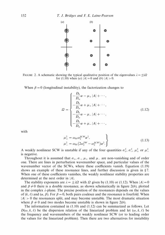
The formulation (2.7) is remarkable in that all three of the operators M, K and L arenon-degenerate, and so they each define canonical symplectic structures on 8.

A fundamental property of the scalar nonlinear wave equation (2.1), that is impor-tant for the existence of short-crested waves, is reversibility in y. If u(x, y, t) is a solu-tion of (2.1), then clearly u(x, −y, t) is also a solution. In the multi-symplectificationof (2.1), this reversibility is defined by the action

R Z(x, y, t) := RZ(x, −y, t) with R = diag(1, 1, 1, −1, −1, −1, 1, −1). (2.8)

The matrix R is an involution (has the property R2 = I) and satisfies

RM = MR, RK = KR, RL = −LR, S(R Z) = S(Z). (2.9)

In turn, the properties (2.9) imply that R Z is a solution of the wave equation in theform (2.7) whenever Z is a solution. The nonlinear wave equation (2.1) is reversible inx and t as well, and a multi-symplectic t-reversor and x-reversor can also be defined,but they are not required in the general theory for short crested waves.

In addition to being a simple example, the nonlinear wave equation has aninteresting property which is quite different from water waves: the determinantcondition (1.14) is not violated. The dispersion relation for (2.1) linearized about thetrivial state u =0 is

D(ω, k, ) = ω2 − k2 − 2 − V ′′(0),

where V ′′(0) > 0 by hypothesis. Hence,

det

Dωω Dωk Dω Dω

Dkω Dkk Dk Dk

Dω Dk D D

Dω Dk D 0

= det

2 0 0 2ω

0 −2 0 −2k

0 0 −2 −2

2ω −2k −2 0

= −16V ′′(0) < 0. (2.10)

Therefore, by choosing V ′′′(0) = 0 and V ′′′′(0) > 0 (since sign(ωkk ωTW2 ) = sign(V ′′′′(0))

in this case), the weakly nonlinear SCWs of (2.1) are stable to long-wave transverseperturbations. They may, of course, still be unstable to short-wave transverseperturbations or longitudinal perturbations.

2.2. Multi-symplectic structure of water waves

The multi-symplectic formulation of water waves of Bridges (1996, 1997a) is used,and the details required are recorded here. Restrict attention to inviscid irrotationalwater waves of constant density on an infinite depth fluid.

Let (x, y) ∈ 2 denote the horizontal coordinates and z the vertical coordinate.Denote by φ(x, y, z, t) the velocity potential. The fluid is bounded above by the surfacez = η(x, y, t). In the interior of the fluid, the velocity potential satisfies Laplace’s


equation

φ = φxx + φyy + φzz = 0 for − ∞ < z < η(x, y, t) (2.11)

and is quiescent far from the surface

∇φ → 0 as z → −∞. (2.12)

At the free surface, the functions (φ, η) satisfy the kinematic and dynamic boundaryconditions

ηt + φxηx + φyηy − φz = 0

φt + 12

(φ2

x + φ2y + φ2

z

)+ gη = 0

at z = η(x, y, t), (2.13)

where g is the gravitational constant.To multi-symplectify, introduce new variables Z = (Φ, η, φ, u, v) where

Φ = φ|z=η, u = φx, v = φy, u = u|z=η, v = v|z=η.

The functions (Φ, η) are, for each (x, y, t), real numbers whereas (φ, u, v) aredependent also on the cross-section z ∈ (−∞, η). Using the fact that

Φt = [φt + φzηt ]|z=η,

with similar relations for Φx and Φy , and the kinematic condition, leads to the identity

Φt + uΦx + vΦy =[φt +

(φ2

x + φ2y + φ2

z

)]∣∣z=η

. (2.14)

With these coordinates, the governing equations can be written in the form

M(Z)Zt + K(Z)Zx + L(Z)Zy = ∇S(Z) (2.15)

with

S(Z) = 12

∫ η

−∞

(u2 + v2 − φ2

z

)dz − 1

2gη2, (2.16)

and the associated side conditions on elements of Z,

φ|z=η = Φ, |∇φ| → 0 as z → −∞. (2.17)

The operators M(Z), K(Z) and L(Z) are defined by

M(Z) =

0 −1 0 0 01 0 0 0 00 0 0 0 00 0 0 0 00 0 0 0 0

, K(Z) =

0 −u 0 0 0u 0 0 0 00 0 0 −1 00 0 1 0 00 0 0 0 0

, (2.18)

and

L(Z) =

0 −v 0 0 0v 0 0 0 00 0 0 0 −10 0 0 0 00 0 1 0 0

. (2.19)

To verify that the right-hand side of (2.15) is the gradient of some functional S,we first introduce a suitable inner product. For vector-valued functions of the type Z,where the first two components are scalar-valued and the last three components are


defined on the cross-section z ∈ (−∞, η), we use the following inner product

〈U, V 〉η = U1V1 + U2V2 +

∫ η

−∞(U3V3 + U4V4 + U5V5) dz. (2.20)

Note that the inner product is dependent on η, and this is indicated by the subscripton the inner product. The gradient of S(Z), (2.16), with respect to the inner product,(2.20), is

∇S(Z)def=

δS/δΦ

δS/δη

δS/δφ

δS/δu

δS/δv

=

−φz|z=η

12

(u2 + v2 + φ2

z

)∣∣z=η

− gη

φzz

u

v

. (2.21)

The water-wave problem has the appropriate y- reversibility that is required for theexistence of SCWs. Let

R = diag(1, 1, I, I, −I).

Then it is easily verified that

RM(R Z) = +M(Z)R, RL(R Z) = +K(Z)R, RL(R Z) = −L(Z)R,

and S(R Z) = S(Z), where R Z = RZ(x, −y, t).The skew-symmetric operators M(Z), K(Z) and L(Z) are non-constant. However,

with a simple transformation, they can be reduced to constant skew-symmetricoperators (see Bridges 2001). Therefore, it will be assumed hereinafter that the water-wave equations are transformed and so are in the standard form (1.1).

The multi-symplectic formulation of water waves is a generalization of the classicalHamiltonian formulation of water waves due to Zakharov (1968). Defining,

∇H (Z) = ∇S(Z) − K(Z)Zx − L(Z)Zy, (2.22)

where ∇ is a gradient operator defined with respect to an inner product that includesintegration over x and y, the equations can be written in the form

M(Z)Zt = ∇H (Z).

This system is the Zakharov formulation rewritten in terms of the Z-variables. Themulti-symplectic structure provides a refinement of the classical Hamiltonian structure,in that it decomposes the Hamiltonian to generate independent symplectic structuresfor the x- and y-directions.

3. The general oblique two-wave interactionMotivated by the nonlinear wave equation and the water-wave problem, the starting

point for the analysis is the general class of abstract Hamiltonian PDEs of the form

MZt + KZx + LZy = ∇S(Z), Z ∈ , (3.1)

under the hypotheses that M, K and L are any constant skew-symmetric operators,S is any given smooth function, which does not depend explicitly on x, y or t . Thelinear space is either n or in the case of water waves it is an inner product spaceof functions in the z-direction. The precise specification of is not required in thesequel. On , the standard inner product will be denoted by 〈·, ·〉.


It is also assumed that there is a reversibility in y with a multi-symplectic action ofthe reversor:

RZ(x, y, t) = RZ(x, −y, t), (3.2)

for some linear operator R : → which is involutive (i.e. R2 = I) and preserves theinner product, and satisfies (2.9) for (3.1). In this setting, an abstract definition of ashort-crested wave can be given (see Appendix A).

In this section, the general two-wave interaction is considered; that is, generalsolutions of (3.1) of the form

Z(x, y, t) = Z(θ1, θ2) where θj = kjx + jy + ωj t (j = 1, 2), (3.3)

and Z is a 2π-periodic function of θ1 and θ2. There is an arbitrary phase shift in eachθj which is suppressed for brevity.

In addition to its importance as an embedding for SCWs, the oblique two-waveinteraction has independent interest in remote-sensing stochastic models, and a modelfor the double-peaked power spectrum observed in shallow water-wave dynamicsLonguet-Higgins 1962; Willebrand 1975; Weber & Barrick 1977; Pierson 1993;Elfouhaily et al. 2000 and references therein).

The main result of this section is a constrained variational principle for the two-wave interaction which generalizes previous variational principles for quasi-periodicpatterns (Bridges 1998) and collinear two-phase wavetrains (Bridges & Laine-Pearson2001). Variational principles can be derived for SCWs directly, as in Bridges, Dias &Menasce (2001) for example, but these variational principles for SCWs do not containenough information for a stability analysis.

The solutions Z(θ1, θ2) can also be interpreted as steady waves travelling in someoblique direction (Milewski & Keller 1996). Let

Θ1 =2θ1 − 1θ2

k12 − k21

, Θ2 =k2θ1 − k1θ2

k12 − k21

.

Then clearly,

Θ1 = x − cxt, Θ2 = y − cyt, with (cx, cy) =

(ω21 − ω12

k12 − 1k2

,ω2k1 − ω1k2

k12 − 1k2

).

The transformation (θ1, θ2) → (Θ1, Θ2) is invertible if k12 − k21 = 0. Note that thisnon-degeneracy condition holds even in the SCW limit (reducing to k = 0). Intransformed coordinates, a doubly periodic wave can be expressed in the form

Z(θ1, θ2) = W (Θ1, Θ2) = W (x − cxt, y − cyt),

i.e. a steady wave travelling with phasespeed vector c=(cx, cy). However, for the varia-

tional characterization, the primitive form of Z(θ1, θ2) is used as the parameter struc-ture is more useful.

The extension from SCWs to the non-resonant two-wave interaction takes aresonant wave to a non-resonant wave, and therefore we would expect small divisors.However, it is not this embedding that gives rise to small divisors, because thereis a continuous symmetry (the translation invariance in the y-direction on periodicfunctions gives an O(2) symmetry), and so the variation of the frequencies and wave-numbers is smooth. In finite dimensions this is reminiscent of the spherical pendulum,and in infinite dimensions it is reminiscent of the similar issues with standing wavesand their embedding in a collinear two-wave interaction (see Bridges & Laine-Pearson2004 for further discussion of this issue).


On the other hand, there is an intrinsic issue of small divisors that arises owing to thecountable number of pure imaginary eigenvalues in the spectrum of the linearizationabout the trivial state. See Craig & Nicholls (2002, § 4.4), for a discussion of this issuefor three-dimensional water waves. However, when we consider capillary–gravitythree-dimensional waves instead of pure gravity waves three-dimensional waves, thesmall-divisor issue disappears and a rigorous proof of such doubly periodic wavescan be obtained (Craig & Nicholls 2000).

The governing equation for a general two-wave interaction Z(θ1, θ2) is obtainedfrom (3.1) which transforms to

J1

∂Z

∂θ1

+ J2

∂Z

∂θ2

= ∇S(Z) where Jj = ωjM + kjK + jL. (3.4)

The operators Jj ∂θjare formally gradient operators, and this is the basis of a

variational principle. The product of the skew-symmetric operator Jj and thederivative ∂θj

is symmetric. Therefore the product can define a quadratic form whosegradient then formally recovers the operator.

For j = 1, 2, define the following six functionals for the two interacting waves

Aj (Z) =

∮12

⟨M

∂Z

∂θj

, Z

⟩dθ, Bj (Z) =

∮12

⟨K

∂Z

∂θj

, Z

⟩dθ,

Cj (Z) =

∮12

⟨L

∂Z

∂θj

, Z

⟩dθ where

∮( ) dθ =

1

(2π)2

∫ 2π

0

∫ 2π

0

( ) dθ1 dθ2.

(3.5)

For the case of water waves, these functionals are expressible in the classical form

Aj (Z) =

∮−Φ

∂η

∂θj

dθ, Bj (Z) =

∮ ∫ η

−∞u

∂φ

∂θj

dz dθ, Cj (Z) =

∮ ∫ η

−∞v

∂φ

∂θj

dz dθ.

(3.6)

The functionals Aj can be identified with a multi-phase form of wave actionand the functionals Bj and Cj can be identified with wave action fluxes (Whitham1974). The difference here is that we do not use a Lagrangian formulation, and theactions and action fluxes have a geometrical characterization (Bridges 1997b). With thegeometrical formulation, the actions and action fluxes enter the linear stability analysisin an explicit way and so stability results can be obtained without having to use amodulation equation such as the multi-phase modulation equation of Ablowitz &Benney (1970).

Consider the Lagrange functional

F(Z; ω, k, ) = S(Z) −2∑

j=1

(ωj Aj +kj Bj +j Cj ) where S(Z) =

∮S(Z) dθ. (3.7)

Then using an inner product that includes integration over θ , the first variation of Fis the governing equation (3.4).

This functional leads to the following constrained variational principle. Let

C(Z) = Z : Aj (Z) = Ij , Bj (Z) = I2+j , Cj (Z) = I4+j , j = 1, 2, I ∈ 6,

where I = (I1, . . . , I6) are assigned level sets of the functionals. Then a two-wave

interaction solution Z(θ1, θ2) can be characterized as a critical point of S with Z

restricted to the set C. The Lagrange necessary condition is ∇F = 0 (3.4).


There are two immediate consequences of the Lagrange multiplier theory. First, thesix parameters (ωj , kj , j ) j = 1, 2 are Lagrange multipliers and therefore satisfy

ω1 =∂S∂I1

, k1 =∂S∂I2

1 =∂S∂I3

ω2 =∂S∂I4

, k2 =∂S∂I5

, 2 =∂S∂I6

. (3.8)

Secondly, the constrained variational principle is non-degenerate if

det

∂ω1

∂I1

∂ω1

∂I2

∂ω1

∂I3

∂ω1

∂I4

∂ω1

∂I5

∂ω1

∂I6

∂k1

∂I1

∂k1

∂I2

∂k1

∂I3

∂k1

∂I4

∂k1

∂I5

∂k1

∂I6

∂1

∂I1

∂1

∂I2

∂1

∂I3

∂1

∂I4

∂1

∂I5

∂1

∂I6

∂ω2

∂I1

∂ω2

∂I2

∂ω2

∂I3

∂ω2

∂I4

∂ω2

∂I5

∂ω2

∂I6

∂k2

∂I1

∂k2

∂I2

∂k2

∂I3

∂k2

∂I4

∂k2

∂I5

∂k2

∂I6

∂2

∂I1

∂2

∂I2

∂2

∂I3

∂2

∂I4

∂2

∂I5

∂2

∂I6

= 0. (3.9)

Using (3.8), the condition (3.9) is equivalent to the non-degeneracy of the Hessian ofS with respect to I1, . . . , I6. A condition which is equivalent to (3.9) is

det

δAδω

δAδk

δAδ

δBδω

δBδk

δBδ

δCδω

δCδk

δCδ

= 0, (3.10)

where

δAδω

=

∂A1

∂ω1

∂A1

∂ω2

∂A2

∂ω1

∂A2

∂ω2

,δAδk

=

∂A1

∂k1

∂A1

∂k2

∂A2

∂k1

∂A2

∂k2

,δAδ

=

∂A1

∂1

∂A1

∂2

∂A2

∂1

∂A2

∂2

, (3.11)

with analogous 2 × 2 matrices for B and C.It follows from the variational principle that the matrices in (3.9) and (3.10) are

symmetric. Hence

δBδω

=δAδk

T

,δCδω

=δAδ

T

,δCδk

=δBδ

T

. (3.12)

Although we have restricted attention to the two-wave interaction here, it shouldbe apparent that the basic formulation can be generalized to N -wave interactions.When there are N interacting waves, there will be 3N functionals and 3N Lagrangemultipliers. For the case of the three-wave interaction of water waves, this variationalprinciple has been applied by Laine-Pearson (2002) to obtain results for the weaklynonlinear three-wave interaction.


4. Weakly nonlinear oblique two-wave interaction of water wavesIn this section, the variational principle of § 3 is applied to weakly nonlinear water

waves. The motivation is twofold: to derive existing results in the literature on the two-wave interaction (e.g. Longuet-Higgins 1962; Weber & Barrick 1977; Pierson 1993)from a variational perspective, and secondly, to obtain information which is used forthe limit to SCWs. Some generalities about the weakly nonlinear two-wave interactionare also discussed.

At the linear level, a two-wave interaction solution of (3.1) is of the form

Z(θ1, θ2) =

2∑j=1

(Aj ξ j exp(iθj ) + c.c.) with D(ωj , kj , j ) = 0, j = 1, 2,

for any complex numbers A1 and A2, where ξ j is an eigenvector and D(ω, k, ) is the

dispersion function. For gravity water waves in infinite depth, D(ω, k, ) = ω2 −g

√k2 + 2.

The simplest nonlinear problem of pairwise interaction is then to study the persist-ence of such a wave interaction in the nonlinear problem for small amplitude. Suchan interaction will not persist for all (A1, A2) ∈ 2 and one purpose of a weaklynonlinear analysis is to determine under what conditions we can expect such aninteraction to persist. The weakly nonlinear theory leads to a set of amplitudeequations of the form

0 = A1(D(ω1, k1, 1) + Λ11|A1|2 + Λ12|A2|2 + · · ·),0 = A2(D(ω2, k2, 2) + Λ21|A1|2 + Λ22|A2|2 + · · ·),

(4.1)

with Λ12 = Λ21. These equations generalize the amplitude equations (1.6) for SCWsto amplitude equations for the two-wave interaction. Here we give a brief account ofthe derivation of this equation for weakly nonlinear two-wave interaction for waterwaves.

According to the variational principle, the solutions correspond to critical points ofS restricted to level sets of the functionals (Aj , Bj , Cj ) for j = 1, 2. The necessarycondition for the variational principle is to find critical points of the unconstrainedfunctional (3.7). We seek solutions that are 2π-periodic in θ1 and θ2 through a doubleFourier series of the form

Z(θ1, θ2) =∑

(m,n)∈2

Zmn exp(i(mθ1 + nθ2)).

Since Z = (Φ, η, φ, u, v)T we can determine Φ , u and v from φ and η using

Φ = φ|z=η,

(u

v

)=

(k1 k2

1 2

)(∂φ/∂θ1

∂φ/∂θ2

).

The problem is then reduced to solving for the velocity potential and free-surfaceelevation. A leading-order expansion for them is

η(θ1, θ2) = A1 eiθ1 + A2 eiθ2 + a21 + a22 e2iθ1 + a23 e2iθ2

+ a24ei(θ1+θ2) + a25 ei(θ1 − θ2) + c.c. + · · · ,

φ(z, θ1, θ2) = b1 eυ1z+iθ1 + b2 eυ2z+iθ2 + b22 e2(υ1z+iθ1) + b23 e2(υ2z+iθ2)

+ b24 eχ+z+i(θ1+θ2) + b25 eχ−z+i(θ1−θ2) + c.c. + · · · ,


where

υ1 =(k2

1 + 21

)1/2, χ+ = [(k1 + k2)

2 + (1 + 2)2]1/2,

υ2 =(k2

2 + 22

)1/2, χ− = [(k1 − k2)

2 + (1 − 2)2]1/2.

Define cos γ = (k1k2 + 12)/(υ1υ2). The angle γ is the angle between the wave vectors(k1, 1) and (k2, 2). In terms of γ ,

χ2+ = υ2

1 + υ22 + 2 cos γ υ1υ2, χ2

− = υ21 + υ2

2 − 2 cos γ υ1υ2.

The above expressions for η, φ, Φ , u and v are substituted into the definitions ofthe functionals S, Aj , Bj and Cj for j = 1, 2 in order to construct the functionalF(a1, b1, . . . , ω, k, ). The Fourier coefficients b1, b2, . . . and a22, a23, . . . are eliminatedusing

∂F∂b1

= 0,∂F∂b2

= 0, . . . ,∂F∂a22

= 0,∂F∂a23

= 0, . . . ,

resulting in a21 = 0 to leading order and

b1 = iω1

υ1

A1 + · · · ,

b22 = 0 + · · · ,b24 = ib24 A1A2 + · · · ,a22 =υ1 A2

1 + · · · ,a24 = a24 A1A2 + · · · ,

b2 = iω2

υ2

A2 + · · · ,

b23 = 0 + · · · ,b25 = ib25 A1A2 + · · · ,a23 = υ2 A2

2 + · · · ,a25 = a25 A1A2 + · · · ,

where

a24 = 14χ+K+ + (υ1 + υ2) − 2

gω1ω2 sin2 1

2γ,

a25 = 14χ−K− + (υ1 + υ2) +

2

gω1ω2 cos2 1

2γ,

b24 = 14(ω1 + ω2)K+,

b25 = 14(ω1 − ω2)K−,

and

K+ =16ω1ω2 sin2 1

2γ

[gχ+ − (ω1 + ω2)2], K− = −

16ω1ω2 cos2 12γ

[gχ− − (ω1 − ω2)2].

Back substitution into F results in the reduced functional

F(|A1|2, |A2|2, ω, k, ) =

(ω2

1

υ1

− g

)|A1|2 +

(ω2

2

υ2

− g

)|A2|2 +

− 2υ1ω21|A1|4 − 2υ2ω

22|A2|4 + Υ |A1|2|A2|2 + · · · , (4.2)

where

Υ =ω1ω2

g(ω1 + ω2)

2K+ sin2 12γ − ω1ω2

g(ω1 − ω2)

2K− cos2 12γ

− 8ω1ω2(υ1 + υ2) cos γ +2

gω2

1ω22(3 + cos2 γ ). (4.3)


Taking the gradient of F with respect to A1 and A2 results in[(ω2

1/υ1 − g)

− 4υ1ω21|A1|2 + Υ |A2|2 + · · ·

]A1 = 0,[(

ω22/υ2 − g

)+ Υ |A1|2 − 4υ2ω

22|A2|2 + · · ·

]A2 = 0,

(4.4)

which is in the standard form (4.1).First note that if |A2| =0 and |A1| =0 or |A1| =0 and |A2| = 0, we recover the weakly

nonlinear dispersion relation for a plane monochromatic wave. When |A1| · |A2| = 0the nonlinear frequency change as a function of amplitude for the (generically) quasi-periodic two-wave interaction is obtained.

The coefficients in (4.4) agree with existing results on the two-wave interaction(Longuet-Higgins 1962; Weber & Barrick 1977; Willebrand 1975; Pierson 1993), andwhen the SCW limit is taken, the coefficient Υ reduces to the coefficient b in (1.6)for SCWs which agrees with the expression for SCWs in Bridges, Dias & Menasce(2001) (denoted α3 on their p. 165). An explicit expression for the SCW limit of Υ isgiven in § 9.

5. Linear stability problem for the oblique two-wave interactionTake the governing equations in the form (3.1) and suppose there exists a smooth

six-parameter family of two-phase waves as in § 3. Consider a perturbation of this

basic state of the form Z → Z +Z and linearize (3.1) about the basic state. The resultis the linear system of PDEs

M∂Z

∂t+ K

∂Z

∂x+ L

∂Z

∂y= HessZS(Z)Z, (5.1)

where HessZS(Z) is the Hessian of S(Z) evaluated at Z.Consider the following class of perturbations

Z(θ1, θ2, x, y, t) = ReU (θ1, θ2) ei(αx+βy+Ωt)

, (5.2)

with α and β real, Ω ∈ , and U (θ1, θ2) a 2π-periodic function of θ1 and θ2.Substitution results in the following eigenvalue problem for the stability exponentΩ ∈ ,

LU = iΩ MU + iα KU + iβ LU (5.3)

where

L = HessZS(Z) − J1

∂

∂θ1

− J2

∂

∂θ2

= HessZS(Z) − ω1M∂

∂θ1

− ω2M∂

∂θ2

− k1K∂

∂θ1

− k2K∂

∂θ2

− 1L∂

∂θ1

− 2L∂

∂θ2

= HessZF(Z), (5.4)

using (3.4) and the definition of F in (3.7).Attention will be restricted to long-wave instabilities where |α|2 + |β|2 1. This

hypothesis does not put any restriction on the amplitude of the basic state, it restrictsonly the class of perturbations. When α = β = 0, the eigenvalue problem for Ω has(at least) a double zero eigenvalue because the kernel of L is non-trivial. The strategyis to expand the solution of (5.3) in a Taylor series in α and β . Then a solvabilitycondition will lead to the leading-order behaviour of the stability exponent.


When Ω = α = β = 0, (5.3) has two solutions,

Ker(L) = spanψ1, ψ2 where ψ j =∂Z

∂θj

for j = 1, 2.

This follows since differentiation of (3.4) with respect to θ1 and θ2 results in

L(∂θjZ) = 0, j =1, 2. Therefore Ker(L) ⊇ spanψ1, ψ2. For particular parameter

values (or with additional symmetry), the kernel may be larger, but generically wehave equality, and this is assumed hereinafter.

The general solution of (5.3) can be expressed in the following form to leadingorder

U = c1U1 + c2U2

= c1

(ψ1 + iα

∂Z

∂k1

+ iβ∂Z

∂1

+ iΩ∂Z

∂ω1

)

+ c2

(ψ2 + iα

∂Z

∂k2

+ iβ∂Z

∂2

+ iΩ∂Z

∂ω2

)+ O(|Ω |2 + |α|2 + |β|2), (5.5)

where (c1, c2) are at present arbitrary complex constants whose properties are tobe determined as part of the analysis. This form of the leading-order solution isconfirmed by noting that differentiation of (1.1) results in

L(

∂Z

∂ωj

)=Mψ j , L

(∂Z

∂kj

)= Kψ j , L

(∂Z

∂j

)= Lψ j for j = 1, 2.

An expression for the stability exponent is obtained by using (5.5) and applyingthe solvability condition to (5.3). Introduce the following inner product for functionsZ ∈ that are 2π-periodic in θ1 and θ2,

[[U, V ]] =

∮〈U (θ1, θ2), V (θ1, θ2)〉 dθ =

1

(2π)2

∫ 2π

0

∫ 2π

0

〈U (θ1, θ2), V (θ1, θ2)〉 dθ1 dθ2, (5.6)

where 〈·, ·〉 is the inner product on . Since Ker(L) = spanψ1, ψ2 by hypothesisand L is formally symmetric, we have the following two solvability conditions for(5.3),

[[ψ j , (iαK + iβL + iΩM)U ]] = 0 for j = 1, 2. (5.7)

However, since (5.3) is linear and U = c1U1 + c2U2, the solvability condition isequivalent to

N(Ω, α, β) c = 0,

where N(Ω, α, β) is the 2 × 2 matrix

N(Ω, α, β)

=

[[ψ1, (iαK + iβL + iΩM)U1]] [[ψ1, (iαK + iβL + iΩM)U2]]

[[ψ2, (iαK + iβL + iΩM)U1]] [[ψ2, (iαK + iβL + iΩM)U2]]

and c =

(c1

c2

).

The matrix N(Ω, α, β) has complex-valued entries dependent on Ω ∈ and (α, β) ∈2. Clearly, there is a non-trivial solution, i.e. ‖c‖ = 0, of the linear stability problemif and only if

(Ω, α, β)def= det[N(Ω, α, β)] = 0. (5.8)


This leads to the following definition of instability: If for some (α, β) ∈ 2 there existsan Ω ∈ such that (Ω, α, β) = 0 and Im(Ω) = 0 the basic state is linearly unstable.

An unstable eigenfunction is constructed as follows. For some (α, β), suppose(Ω, α, β) has an unstable root Ω . Then substitute this (α, β, Ω) into the expressionfor U (θ1, θ2) which in turn is substituted into the expression for the perturbation(5.2). The resulting function Z(θ1, θ2, x, y, t) is then an approximation to an unstableeigenfunction of (5.1), valid for |Ω |, |α| and |β| sufficiently small.

The expression for U in (5.5) is used to construct the leading-order Taylor expansionof N(Ω, α, β), and hence (Ω, α, β), to obtain a sufficient condition for linearinstability valid for |Ω |2 + |α|2 + |β|2 sufficiently small.

Our main result is that the matrix N can be expressed in terms of known quantities.First, the expression will be given, and then it will be verified,

N(Ω, α, β) = N0 + N1Ω + N2Ω2 + o(|Ω |2 + |α|2 + |β|2), (5.9)

with

N0 = α2 δBδk

+ αβ

(δBδ

+δCδk

)+ β2 δC

δ,

N1 = α

(δAδk

+δBδω

)+ β

(δAδ

+δCδω

),

N2 =δAδω

,

(5.10)

where the matrices δA/δω etc. are defined in (3.11). The Jacobians from the varia-tional principle of § 3 appear in a central way in the analysis of long-wave instability:the leading-order terms in the stability problem can be obtained from known infor-mation about the basic state.

The derivation of the entries of the matrix N2 is given, with the verification of theother two following the same argument. By definition

N(Ω, 0, 0) =

iΩ[[ψ1, MU1]] iΩ[[ψ1, MU2]]

iΩ[[ψ2, MU1]] iΩ[[ψ2, MU2]]

.

Substitute the leading-order expression for U1 and U2 from (5.5),

N(Ω, 0, 0) =

iΩ[[ψ1, M(ψ1 + iΩZω1)]] iΩ[[ψ1, M(ψ2 + iΩZω2

)]]

iΩ[[ψ2, M(ψ1 + iΩZω1)]] iΩ[[ψ2, M(ψ2 + iΩZω2

)]]

= Ω2

[[Mψ1, Zω1]] [[Mψ1, Zω2

]]

[[Mψ2, Zω1]] [[Mψ2, Zω2

]]

,

where we have used the identities [[ψ i , Mψ j ]] = 0 for i, j = 1, 2. Now, let Aj (Z) bethe actions (3.5) evaluated at the basic state. Then

δAδω

=

∂A1

∂ω1

∂A1

∂ω2

∂A2

∂ω1

∂A2

∂ω2

=

[[M∂θ1Z, ∂ω1

Z]] [[M∂θ1Z, ∂ω2

Z]]

[[M∂θ2Z, ∂ω1

Z]] [[M∂θ2Z, ∂ω2

Z]]

.


Comparing the above two results proves that

N(Ω, 0, 0) = Ω2 δAδω

.

The leading-order part of N in (5.9) is of the form of a lambda matrix (Lancaster1966). Solving for the Ω roots, is equivalent to solving the nonlinear in the parametereigenvalue problem,

[N0 + N1Ω + N2Ω2]c = 0,

for the eigenvalue Ω and eigenvector c. These quadratic eigenvalue problems fre-quently arise in the theory of vibrating systems in mechanics. This quadratic eigenvalueproblem is equivalent (when det(N2) = 0) to the problem of finding the eigenvalues Ω

of the classical generalized symmetric eigenvalue problem[(0 N2

N2 N1

)Ω +

(−N2 00 N0

)](dc

)=

(00

)(Lancaster 1966, pp. 58–59). However, we have found no advantage to studying thislinear eigenvalue problem, rather than the nonlinear form.

The main result of this section is: given a basic state (Z, ω1, k1, 1, ω2, k2, 2), thereare accompanying Jacobian matrices δA/δω, . . . , δC/δ which arise naturally in thevariational principle of § 3, and the long-wave instability is completely determinedby these Jacobian matrices. This stability result is for the general oblique two-waveinteraction. A special case is a stability result for SCWs.

6. The stability quartic for long-wave instabilitiesExpanding the determinant (Ω, α, β) leads to a quartic polynomial for the stability

exponent Ω

(Ω, α, β) = det[N0 + N1Ω + N2Ω2] = g4Ω

4 + g3Ω3 + g2Ω

2 + g1Ω + g0, (6.1)

where

g4 =det

(δAδω

),

g3 = tr

[(δAδω

)(α

[δAδk

+δBδω

]+ β

[δAδ

+δCδω

])],

g2 =det

(α

[δAδk

+δBδω

]+ β

[δAδ

+δCδω

])+ tr

[(δAδω

)(α2 δB

δk+ αβ

[δBδ

+δCδk

]+ β2 δC

δ

)],

g1 = tr

[(α2 δB

δk+ αβ

[δBδ

+δCδk

]+ β2 δC

δ

)(α

[δAδk

+δBδω

]+ β

[δAδ

+δCδω

])],

g0 =det

(α2 δB

δk+ αβ

[δBδ

+δCδk

]+ β2 δC

δ

).

(6.2)

where tr( ) is the trace, and the superscript indicates adjugate. The it adjugate ofa matrix is the transpose of the cofactor matrix. If a matrix R is invertible thenR = det(R)R−1.


τ3

τ2 τ1

Figure 4. The discriminant surface for the quartic.

Dividing through the quartic by g4 and introducing the transformation Ω = X −(g3/4)/g4 reduces the quartic to standard form,

(X) = X4 + τ1X2 + τ2X + τ3,

with

τ1 =1

g24

(− 3

8g2

3 + g4g2

),

τ2 =1

g34

(18g3

3 − 12g4g3g2 + g2

4g1

),

τ3 =1

g44

(− 3

256g4

3 + 116

g4g23g2 − 1

4g2

4g3g1 + g34g0

),

(6.3)

Since g3 and g4 are real, the Im(Ω) = 0 if and only if Im(X) = 0. Therefore, we canappeal to standard results for the quartic to determine when there is at least one zeroof (X) with non-zero imaginary part.

There are three diagnostic functions

d1 = τ1, d2 = Discriminant, d3 = τ 21 − 4τ3.

where Discriminant = 16τ3τ41 − 4τ 2

2 τ 31 − 128τ 2

3 τ 21 + 144τ 2

2 τ3τ1 − 27τ 42 + 256τ 3

3 . Theconditions for instability (the existence of at least one root with non-zero imaginarypart) are

d1 > 0 or d1 < 0, d2 < 0 or d1 < 0, d2 > 0, d3 < 0. (6.4)

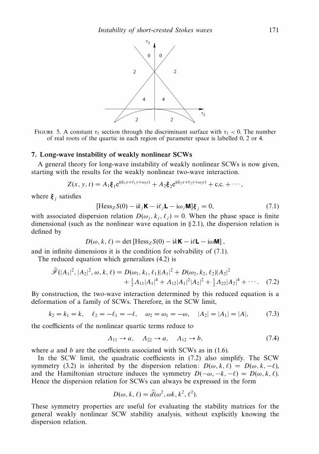
The discriminant surface is plotted in τ space in figure 4. If τ1 > 0 it is immediatethat there is at least one unstable eigenvalue. When τ1 < 0 we must check additionaldiagnostics. A section through the discriminant surface for τ1 < 0 is shown in figure 5.Unless τ2 and τ3 are in the enclosed central region (marked with a 4 in the figure)there is a root which is unstable (having a non-zero imaginary part).

Therefore, given a basic state with associated Jacobian matrices, the problem oflong-wave instability reduces to checking the above conditions on the quartic. Theproblem of long-wave instability for SCWs reduces to checking the above conditions –after the SCW limit is taken. This programme will be carried out for weakly nonlinearSCWs in the next section.


0 0

τ2

τ3

2 2

22

4 4

Figure 5. A constant τ1 section through the discriminant surface with τ1 < 0. The numberof real roots of the quartic in each region of parameter space is labelled 0, 2 or 4.

7. Long-wave instability of weakly nonlinear SCWsA general theory for long-wave instability of weakly nonlinear SCWs is now given,

starting with the results for the weakly nonlinear two-wave interaction.

Z(x, y, t) = A1ξ 1ei(k1x+1y+ω1t) + A2ξ 2e

i(k2x+2y+ω2t) + c.c. + · · · ,

where ξ j satisfies

[HessZS(0) − ikjK − ijL − iωjM]ξ j = 0, (7.1)

with associated dispersion relation D(ωj , kj , j ) = 0. When the phase space is finitedimensional (such as the nonlinear wave equation in § 2.1), the dispersion relation isdefined by

D(ω, k, ) = det [HessZS(0) − ikK − iL − iωM] ,

and in infinite dimensions it is the condition for solvability of (7.1).The reduced equation which generalizes (4.2) is

F(|A1|2, |A2|2, ω, k, ) = D(ω1, k1, 1)|A1|2 + D(ω2, k2, 2)|A2|2

+ 12Λ11|A1|4 + Λ12|A1|2|A2|2 + 1

2Λ22|A2|4 + · · · . (7.2)

By construction, the two-wave interaction determined by this reduced equation is adeformation of a family of SCWs. Therefore, in the SCW limit,

k2 = k1 = k, 2 = −1 = −, ω2 = ω1 = −ω, |A2| = |A1| = |A|, (7.3)

the coefficients of the nonlinear quartic terms reduce to

Λ11 → a, Λ22 → a, Λ12 → b, (7.4)

where a and b are the coefficients associated with SCWs as in (1.6).In the SCW limit, the quadratic coefficients in (7.2) also simplify. The SCW

symmetry (3.2) is inherited by the dispersion relation: D(ω, k, ) = D(ω, k, −),and the Hamiltonian structure induces the symmetry D(−ω, −k, −) = D(ω, k, ).Hence the dispersion relation for SCWs can always be expressed in the form

D(ω, k, ) = d(ω2, ωk, k2, 2).

These symmetry properties are useful for evaluating the stability matrices for thegeneral weakly nonlinear SCW stability analysis, without explicitly knowing thedispersion relation.


Differentiating F in (7.2) with respect to the amplitudes, results in the followingexpression for the amplitudes to leading order(

|A1|2|A2|2

)= −Λ−1

(D(ω1, k1, 1)D(ω2, k2, 2)

)where Λ =

[Λ11 Λ12

Λ12 Λ22

]. (7.5)

To compute the stability matrices δA/δω, . . . , δC/δ, we take as a starting pointthe abstract form (3.5). To leading order, the general form for Aj , Bj and Cj , j = 1, 2is

Aj =∂D

∂ωj

|Aj |2 + · · · , Bj =∂D

∂kj

|Aj |2 + · · · , Cj =∂D

∂j

|Aj |2 + · · · , (7.6)

where D is a function of (ωj , kj , j ), and the amplitudes |Aj | are considered functionsof (ω, k, ) through (7.5).

The details of the construction and limit process for δA/δω are given, and thenthe results for the other stability matrices is summarized,

δAδω

=

∂A1

∂ω1

∂A1

∂ω2

∂A2

∂ω1

∂A2

∂ω2

= −

∂ω1D(ω1, k1, 1) 0

0 ∂ω2D(ω2, k2, 2)

Λ−1

∂ω1D(ω1, k1, 1) 0

0 ∂ω2D(ω2, k2, 2)

+

∂ω1ω1D(ω1, k1, 1)|A1|2 0

0 ∂ω2ω2D(ω2, k2, 2)|A2|2

+ · · · . (7.7)

Hereinafter all expressions are evaluated at the SCW limit in (7.3)–(7.4). EvaluatingδA/δω in this limit,

δAδω

= −(Dω)2(Λ)−1 + Dωω|A|2(

1 00 1

)+ · · · . (7.8)

The other stability matrices in the SCW limit are

δAδk

= −DωDkΛ−1 + Dωk|A|2

(1 00 1

)+ · · · ,

δAδ

= −DωDΛ−1

(1 00 −1

)+ Dω|A|2

(1 00 −1

)+ · · · ,

δBδk

= −D2kΛ

−1 + Dkk|A|2(

1 00 1

)+ · · · ,

δBδ

= −DkDΛ−1

(1 00 −1

)+ Dk|A|2

(1 00 −1

)+ · · · ,

δCδ

= −D2

1|Λ|Λ + D|A|2

(1 00 1

)+ · · · ,

(7.9)

with the other matrices given by the symmetry relations (3.12).


We are now in a position to compute the coefficients of the stability quartic(6.1)–(6.2),

(Ω, α, β) = g4Ω4 + g3Ω3 + g2Ω

2 + g1Ω + g0, (7.10)

with

g4 =D4

ω

|Λ| − 2aDωωD2

ω

|Λ| |A|2 + D2ωω|A|4 + · · · ,

g3 = 4α

[D3

ωDk

|Λ| − aDω

|Λ| (DωDωk + DωωDk)|A|2 + DωωDωk|A|4]

+ · · · ,

g2 = 2D2

ω

|Λ|(3α2D2

k − β2D2

)− 2a

|Λ|[α2

(4DωDkDωk + D2

ωDkk + DωωD2k

)+β2

(− 4DωDDω + DωωD2

+ D2ωD

)]|A|2

+ 2[α2

(2D2

ωk + DωωDkk

)+ β2

(DωωD − 2D2

ω

)]|A|4 + · · · ,

g1 =4

|Λ| [−αDωDk(βD − αDk)(βD + αDk)]

− 4a

|Λ|[α3(DkDωk + DωDkk)Dk

+αβ2(DDωDk + D2

Dωk − 2D[DkDω+ DkDω])]

|A|2

+ 4α[α2DkkDωk + 2β2(DDωk − DkDω)]|A|4 + · · · ,

g0 =1

|Λ| (βD − αDk)2(βD + αDk)

2 +

− 2a

|Λ|[α4DkkD

2k + α2β2

(D2

Dkk + D2kD − 4DDkDk

)+ β4D2

D

]|A|2

+ (α2Dkk − 2αβDk + β2D)(α2Dkk + 2αβDk + β2D)|A|4 + · · · .

Details of the calculation of these coefficients can be found in Laine-Pearson (2002).The only place that the coefficient b in the frequency correction to SCWs appears

in the coefficients is in |Λ| = a2 − b2. Multiplying (Ω, α, β) by |Λ| shows that theeffect of b does not appear in the coefficients at order |A|0 or |A|2, but appears in theterms of order |A|4.

In the zero-amplitude limit, the stability quartic (7.10) has a nice factorization

(Ω, α, β) =1

|Λ| (DωΩ + Dkα + Dβ)2 (DωΩ + Dkα − Dβ)2 . (7.11)

It is clear from this expression that the hypotheses

Dω = 0, Dk = 0, D = 0, (7.12)

when evaluated at the SCW frequency and wavenumbers, are required to avoiddegeneracy. When the conditions (7.12) are not satisfied, it is an indication thatresonances or other degeneracies of the dispersion relation will occur.

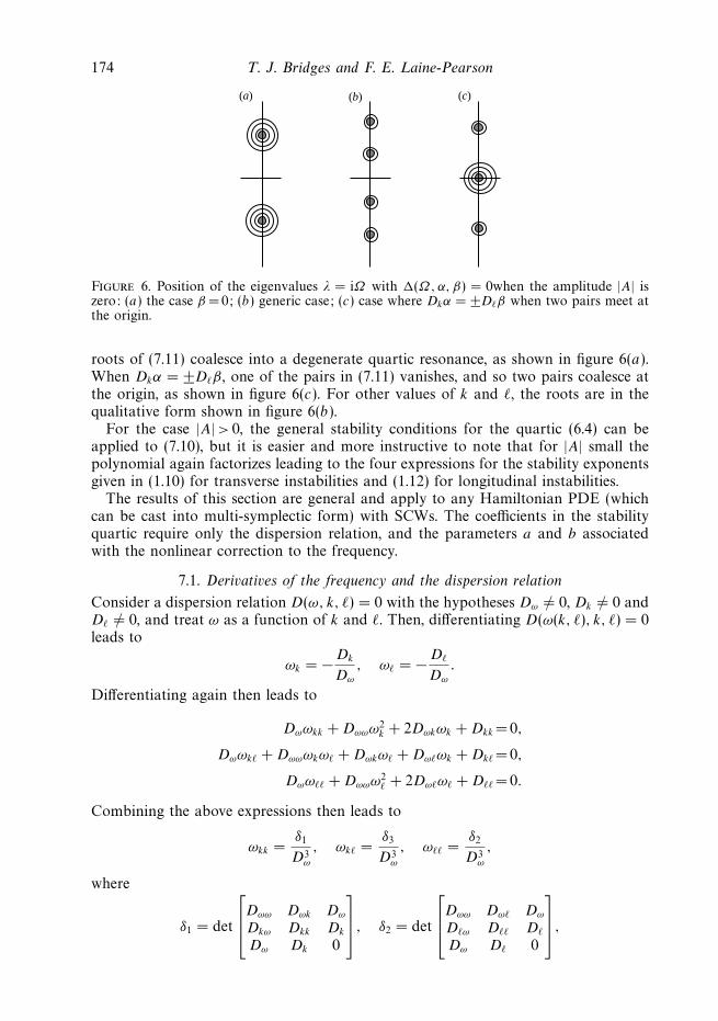
The eight eigenvalues λ = ±iΩ with Ω a root of (7.11) are purely imaginary andare grouped into four pairs. Their location on the imaginary axis depends on thevalues of k and . In figure 6, the principal cases are shown. When β = 0, the four


(b)(a) (c)

Figure 6. Position of the eigenvalues λ = iΩ with (Ω,α, β) = 0when the amplitude |A| iszero: (a) the case β =0; (b) generic case; (c) case where Dkα = ±Dβ when two pairs meet atthe origin.

roots of (7.11) coalesce into a degenerate quartic resonance, as shown in figure 6(a).When Dkα = ±Dβ , one of the pairs in (7.11) vanishes, and so two pairs coalesce atthe origin, as shown in figure 6(c). For other values of k and , the roots are in thequalitative form shown in figure 6(b).

For the case |A| > 0, the general stability conditions for the quartic (6.4) can beapplied to (7.10), but it is easier and more instructive to note that for |A| small thepolynomial again factorizes leading to the four expressions for the stability exponentsgiven in (1.10) for transverse instabilities and (1.12) for longitudinal instabilities.

The results of this section are general and apply to any Hamiltonian PDE (whichcan be cast into multi-symplectic form) with SCWs. The coefficients in the stabilityquartic require only the dispersion relation, and the parameters a and b associatedwith the nonlinear correction to the frequency.

7.1. Derivatives of the frequency and the dispersion relation

Consider a dispersion relation D(ω, k, ) = 0 with the hypotheses Dω = 0, Dk = 0 andD = 0, and treat ω as a function of k and . Then, differentiating D(ω(k, ), k, ) = 0leads to

ωk = − Dk

Dω

, ω = − D

Dω

.

Differentiating again then leads to

Dωωkk + Dωωω2k + 2Dωkωk + Dkk = 0,

Dωωk + Dωωωkω + Dωkω + Dωωk + Dk = 0,

Dωω + Dωωω2 + 2Dωω + D = 0.

Combining the above expressions then leads to

ωkk =δ1

D3ω

, ωk =δ3

D3ω

, ω =δ2

D3ω

,

where

δ1 = det

Dωω Dωk Dω

Dkω Dkk Dk

Dω Dk 0

, δ2 = det

Dωω Dω Dω

Dω D D

Dω D 0

,


and

δ3 = DωDkDω + DωkDDω − DωωDDk − DkD2ω.

Combining these expressions leads to the formula

−D4ω det

(ωkk ωk

ωk ω

)= det

Dωω Dωk Dω Dω

Dkω Dkk Dk Dk

Dω Dk D D

Dω Dk D 0

, (7.13)

which we have not seen in the literature. The proof of this formula follows from adirect calculation.

The sign of the determinant in (7.13) is independent of the choice of coordinatesin the following sense. The dispersion function D(ω, k, ) is not unique. Any otherfunction E(ω, k, ) with the same zeros, say E(ω, k, ) = d(ω, k, )D(ω, k, ) for somenon-vanishing function d(ω, k, ) is also a dispersion function. However, it is easy toshow that the determinant (7.13) based on any other dispersion function E(ω, k, )has the same sign as the determinant based on D(ω, k, ).

8. Transverse instabilities of weakly nonlinear short-crested water wavesIn this section, expressions for the stability exponents are explicitly computed for

weakly nonlinear short-crested gravity water waves on an infinite depth fluid when β

is small, but outside a neighbourhood of β = 0.The dispersion relation for water waves is given in (1.17). The coefficient a for

water waves is strictly negative, and

det

Dωω Dωk Dω Dω

Dkω Dkk Dk Dk

Dω Dk D D

Dω Dk D 0

= det

2 0 0 2ω

0 −g2

ν3

gk

ν3−gk

ν

0gk

ν3−gk2

ν3−g

ν

2ω −gk

ν−g

ν0

= 2

ω6

ν4> 0. (8.1)

The Hessian of ω with respect to k and has the simple form[ωkk ωk

ωk ω

]=

g

4ων3

[22 − k2 −3k

−3k 2k2 − 2

]=

ω

4ν4

[ k

−k

]2 00 −1

[ −k

k

].

By applying (1.14) to (8.1), it is immediate that weakly nonlinear SCWs are unstableto long-wave perturbations.

The dependence of the transverse instabilities on the perturbation wavenumbers(α, β) is obtained from (1.10). For water waves the stability exponents are λ = ±iΩwith

Ω =

g

2νω(kα + β) − σ+|A| + · · · ,

g

2νω(kα + β) + σ+|A| + · · · ,

g

2νω(kα − β) − σ−|A| + · · · ,

g

2νω(kα − β) + σ−|A| + · · · ,

(8.2)

with σ+ and σ− defined in (1.19).


Figure 7. Position of unstable modes for each wedge in the (α, β)-plane when (a) 0 <

< 1/√

2k, (b) 1/√

2k < <√

2k, (c) >√

2k. In terms of the angle of incidence θ (see (8.3)for a definition) these regions correspond to (a) 54.73 < θ < 90, (b) 35.26 < θ < 54.73, (c)0 < θ < 35.26.

For all admissible values of k and for SCWs there are unstable wedges in the(α, β)-plane. However, the properties of these instabilities depend on the values ofk and . There are three regions in (k, ) space and for each of these regions theunstable wedges in the (α, β)-plane are shown in figure 7.

For weakly three-dimensional SCWs, that is; when is small (and 2 < k2/2), thereare two unstable wedges, a as shown in figure 7(a). In the lower unstable wedge,there are two unstable modes and in the middle wedge, there is one unstable mode(as shown in figure 3).

In the intermediate region, when 1/k22, < 2 < 2k2, there is only one unstable wedge,as shown in figure 7(b), and it has only one unstable mode. In the large region,where 2 > 2k2, there are again two unstable wedges with the higher wedge (darkershading) now having two unstable modes, as shown in figure 7(c). The location ofthe unstable wedges in figure 7(c) is the reverse of that in figure 7(a).

The results in figure 7 can also be interpreted in terms of a wave reflection off awall. Consider the case of an incident wave of wavelength 2π/ν, where ν =

√k2 + 2,

being fully reflected off a vertical wall. Let k = ν sin θ and = ν cos θ . Then, θ is theangle between the direction of propagation of the incident wave and the normal tothe wall (cf. Roberts 1983). In terms of the angle θ , the critical values in figure 7 are

/k =√

2 ⇒ θ = tan−1(1/√

2) ≈ 35.26,

/k = 1√2

⇒ θ = tan−1(√

2) ≈ 54.73.

(8.3)

The limit θ → 90 corresponds to the limit where the two waves are collinear Stokestravelling waves. Hence, figure 7(a) corresponds the the region closest to the travelling,wave limit. Note that this limit is singular so the results are not valid in the limitθ → 90. Figure 7(a) is consistent with the fact that the Stokes travelling-wave ismodulation unstable, but it also shows a difference from the travelling-wave case: thedarker shaded region has two modes of instability, whereas a Stokes travelling wavewould have only one unstable mode. The limit θ → 0 corresponds to the standing-wave limit. Near θ = 0, the instability regions in figure 7(c) are just the opposite offigure 7(a), with the strongest region of instability predominantly in the y-direction.This limit is consistent with the modulation instability of pure standing waves; further


details of the instability of pure standing waves using the multi-symplectic frameworkcan be found in Bridges & Laine-Pearson (2004).

9. Longitudinal instabilities of weakly nonlinear short-crested water wavesWhen β =0, the leading-order term for the roots of the stability quartic (7.10)

depends also on the terms of order |A|4 in the coefficients. When β = 0 and |A| = 0,the stability quartic (7.10) has a quartic root

(Ω, α, β) =1

|Λ| (DωΩ + Dkα)4.

Hence, the perturbation of this root for |A| = 0 has a leading-order term of the orderof the fourth root of the perturbation. Since the perturbation is of order |A|2, theleading-order expansion for the perturbed quartic root is of the form

Ω = − Dk

Dω

α + Ω1|A|1/2 + Ω2|A| + · · · .

However, owing to symmetry, the term Ω1 = 0 and the leading-order term is of order|A|, but the coefficient Ω2 then depends on the terms of order |A|4 in the coefficients of(7.10). Let δ1 be as defined in § 7.1, then a calculation shows – to leading order in |A| –that the quartic root associated with β = 0 perturbs into the four roots (expressingthe four values of Ω2 as ±µ±)

Ω =

− Dk

Dω

α + µ+|A| + · · ·

− Dk

Dω

α + µ+|A| + · · ·

− Dk

Dω

α − µ−|A| + · · ·

− Dk

Dω

α + µ−|A| + · · · ,

with µ2± = − (a ± b)

D4ω

δ1α2. (9.1)

However, in § 7.1 it was shown that δ1 = ωkkD3ω. Substituting this expression into µ2

±and using the definitions of ωTW

2 and ωSCW2 recovers the expressions in (1.13).

The eight stability exponents are given by λ = ±iΩ , with Ω taking the four valuesabove. Clearly, stability is determined by the signs of µ2

±, and the signs of µ2± are

determined by the signs of (a + b), (a − b) and δ1. With k = ν sin θ and = ν cos θ ,the coefficients a and b (= Υ in (4.3) in the SCW limit) can be expressed in the form

a= −4gν2,

b= 4gν2

(−2 + 6 cos2 θ +

8 cos4 θ

sin θ − 2+ 2 cos4 θ

).

The normalized (divided by 4gν2) expressions for (a + b) and (a − b) are shown infigure 8.

However, longitudinal stability is determined by the the product of (a ± b) withδ1 (or ωkk). The sign of δ1 is determined by the sign of 22 − k2 and this functionis positive for θ small and changes sign when θ ≈ 54.74. Therefore, longitudinalinstability for |A| small is determined by the inequalities

(a + b)(k2 − 22) < 0 or (a − b)(k2 − 22) < 0.


8060

1

040

–1

–2

20

–3

0

Figure 8. Plot of (a + b) and (a − b), normalized by 4g(k2 + 2), as functions of θ . Thedecreasing function is (a + b) and it passes through zero when θ ≈ 21.96. The function (a − b)vanishes when θ ≈ 63.26.

80

6

4

60

2

040

–2

200

Figure 9. Plot of (a + b)(k2 − 22) (the predominantly lower curve) and (a − b)(k2 − 22)as functions of θ .

90~63~55~22 θ

Figure 10. Schematic position in the complex λ-plane of the eigenvalues associatedwith longitudinal instability for each θ region.

The two functions in these inequalities are plotted as functions of θ in figure 9.Instability is signalled when either of the functions in figure 9 is negative.

There are four distinct θ regions separated by the zeros of (a +b), (a −b) and δ1, asshown in figure 10. In the region 0 <θ < 22, there is one (complex conjugate) pair ofunstable eigenvalues; for 22 < θ < 55, all roots are stable. In the region 55 < θ < 63,


there are two pairs of unstable eigenvalues, and then in the region 63 < θ < 90, thereis one pair of unstable eigenvalues.

The two unstable regions 0 <θ < 22 and 63 < θ < 90 agree with the predictions ofRoskes (1976b). The angle used by Roskes is equal to 2(90−θ), so θ ≈ 22 correspondsto Roskes’ 136 and θ ≈ 63 corresponds to Roskes’ 55. However, his analysis missesthe unstable region 55 <θ < 63 because both µ2

± are negative in that region.The qualitative position of the roots for β =0 will persist for β small. Therefore,

we expect the position of the roots in figure 10 to persist in a small wedge aroundthe axis β = 0. This small wedge of longitudinal instabilities is consistent with thenumerical calculations reported in figures 8 and 9 in Ioualalen & Kharif (1994).

9.1. Instability of short-crested capillary–gravity water waves

The addition of capillarity brings new features that are worthy of mention. The issuesare just sketched in this subsection. The first new feature is that a rigorous theory ofexistence for capillary–gravity SCWs – and their deformation into the non-resonanttwo-wave interaction – is available (Craig & Nicholls 2000), suggesting that they aremore robust than pure gravity waves. Indeed, it is conceivable that a rigorous theoryfor instability could also be developed for the case of capillary–gravity SCWs. Thesecond issue is the larger range of possibilities for instability. For example, all thecritical coefficients (the determinant (8.1), and the parameters σ 2

+, σ 2− µ2

− and µ2+) have

additional sign changes in parameter space. A clue to the range of possibilities fortransverse instabilities can be seen from the range of instabilities of oblique capillary–gravity travelling waves (cf. § 5 of Bridges 1996). When capillary forces are ad-ded, the longitudinal instabilities will also change. For example, it is shown inBridges,Dias & Menasce (2001) that the coefficients a and b have sign changes along lines inthe (θ, τ ) plane where τ is the Bond number.

10. Concluding remarksTwo directions in which the theory here can be extended are the stability of SCWs

in shallow water, and the stability of the resonant and non-resonant three-waveinteraction.

The issue with shallow-water and finite-depth SCWs is the mean flow which caninfluence stability. However, the theory presented here can be combined with thetheory in Bridges et al. (2001). The idea would be to couple the six-parametertwo-wave interaction with the three-parameter mean flow in Bridges et al. (2001),leading to a nine-parameter problem. The stability polynomial will be a sixth-orderpolynomial in this case. Theoretically the strategy is clear, but the details will belengthy for this case. There are questions to be tackled, however. It would be of greatinterest to have analytical results for weakly nonlinear SCWs in shallow water, andalso there are open questions about the stability of two-wave interactions in shallowwater (cf. Onorato et al. (2002)).

The resonant and non-resonant three-wave interaction is the next logical step. Thereis enough symmetry (when the three waves are oblique), so the idea of embedding theresonant interaction in a three-phase non-resonant interaction still makes theoreticalsense. In infinite depth this will be a nine-parameter problem, and the stabilitypolynomial will be sixth order. In finite depth, when mean flow effects are accountedfor, there will be twelve parameters, and the stability polynomial will be eighth order.Some results on the weakly nonlinear three-wave interaction of water waves in infinitedepth have been obtained by Laine-Pearson (2002).


The authors are grateful to all three referees for their constructive and usefulsuggestions, and particularly grateful to the referee who encouraged the authors toexamine more closely the nature of the limit β = 0 in the linear stability problem.

Appendix. Some properties of short-crested wave solutions of multi-symplecticPDEs

What precisely is a short-crested Stokes wave? Key features are (a) periodicity inall space directions and time; (b) uniformly travelling; (c) reflection symmetric in thedirection orthogonal to the direction of propagation. In the multi-symplectic setting,the concept of a reversor is used to give a precise definition.

A solution, Z(x, y, t) of (3.1), is called a short-crested wave if it is periodic in x, y

and t , is travelling in the x-direction (depends on x and t in linear combination only)

and satisfies R Z(x, y, t) = Z(x, y, t).An immediate consequence of this definition is that the transverse momentum of

a short-crested wave is identically zero. An application of Noether’s theorem showsthat the appropriate form for the density of the momentum vector is

M =(

12〈MZx, Z〉, 1

2〈MZy, Z〉

).

This form can be verified by using Noether’s theorem, as in the Appendix of Bridges &Laine-Pearson (2004), or by direct calculation as below.

For functions satisfying (3.1), we have the following conservation law for thetransverse momentum

∂

∂t

(12〈MZy, Z〉

)+

∂

∂x

(12〈KZy, Z〉

)+

∂

∂y

(S(Z) − 1

2〈MZt, Z〉 − 1

2〈KZx, Z〉

)= 0,

and soon a space of functions that are periodic in x and y (and normalizing theperiod to 2π in each direction)

My =

∫2

12〈MZy, Z〉 dx dy =

1

(2π)2

∫ 2π

0

∫ 2π

0

12〈MZy, Z〉 dx dy

is conserved in time. For water waves, this functional can be expressed in the form

My =

∫2

−Φηy dx dy.

One implication of the above definition of SCWs is that it implies immediatelythat My – when evaluated on an SCW – is identically zero for all time. This followssince

My(R Z) =

∫2

12〈MR(Z(x, −y, t))y, RZ(x, −y, t)〉 dx dy (by definition),

= −∫

2

12〈MRZy(x, −y, t), RZ(x, −y, t)〉 dx dy,

= −∫

2

12〈RMZy(x, −y, t), RZ(x, −y, t)〉 dx dy (using RM = MR),

= −∫

2

12〈MZy(x, −y, t), Z(x, −y, t)〉 dx dy

(since R preserves the inner product),

= −∫

2

12〈MZy(x, y, t), Z(x, y, t)〉 dx dy

(transforming y → −y and using periodicity),

= −My(Z).

Therefore, if Z(x, y, t) is an SCW and so R Z = Z, it is immediate that My(Z) = 0.


Momentum

Energy SCWs

region

Two-wave

OTW OTW

Figure 11. Location of SCWs and the two-wave interaction in theenergy-(transverse)momentum diagram.

The energy and transverse momentum are useful for distinguishing SCWs fromoblique travelling waves (OTW). OTWs have non-zero transverse momentum. Aschematic of the energy–momentum (transverse) space is shown in figure 11. The twoOTWs correspond to the arms shown, with SCWs along the vertical (zero-momentum)axis. The oblique two-wave interaction then fills out the space between the OTWsand SCWs. The embedding of SCWs in the two-phase wavetrain extends the SCWsinto this two-wave region.

This energy momentum diagram is very similar to the energy-momentum diagramfor the spherical pendulum and for standing waves (cf. Bridges & Laine-Pearson2004).

REFERENCES

Ablowitz, M. J. & Benney, D. J. 1970 The evolution of multi-phase modes for nonlinear dispersivewaves. Stud. Appl. Maths 49, 225–238.

Badulin, S. I., Shira, V. I., Kharif, C. & Ioualalen, M. 1995 On two approaches to the problemof instability of short-crested water waves. J. Fluid Mech. 303, 297–326.

Bridges, T. J. 1996 Periodic patterns, linear instability, symplectic structure and mean-flow dynamicsfor three-dimensional surface waves. Phil. Trans. R. Soc. Lond. A 354, 533–74.

Bridges, T. J. 1997a Multi-symplectic structures and wave propagation. Math. Proc. Camb. Phil.Soc. 121, 147–190.

Bridges, T. J. 1997b A geometric formulation of the conservation of wave action and its implicationsfor signature and the classification of instabilities. Proc. R. Soc. Lond. A 453, 1365–1395.

Bridges, T. J. 1998 Toral-equivariant partial differential equations and quasiperiodic patterns.Nonlinearity 11, 467–500.

Bridges, T. J. 2001 Transverse instability of solitary-wave states of the water-wave problem. J. FluidMech. 439, 255–278.

Bridges, T. J., Dias, F. & Menasce, D. 2001 Steady three-dimensional water-wave patterns on afinite-depth fluid. J. Fluid Mech. 436, 145–175.

Bridges, T. J. & Laine-Pearson, F. E. 2001 Multisymplectic relative equilibria, multiphasewavetrains and coupled NLS equations. Stud. Appl. Maths 107, 137–155.

Bridges, T. J. & Laine-Pearson, F. E. 2004 Nonlinear counterpropagating waves, multi-symplecticgeometry, and the instability of standing waves. SIAM J. Appl. Maths 64, 2096–2120.

Craig, W. & Nicholls, D. P. 2000 Traveling two and three dimensional capillary-gravity waterwaves. SIAM J. Math. Anal. 32, 323–359.

Craig, W. & Nicholls, D. P. 2002 Traveling gravity water waves in two and three dimensions. Eur.J. Mech. B/Fluids 21, 615–641.

Elfouhaily, T., Thompson, D. R., Vandemark, D. & Chapron, B. 2000 Truncated Hamiltonianversus surface perturbation in nonlinear wave theories. Waves Random Media 10, 103–116.


Hsu, J. R. C., Silvester, R. & Tsuchiya, Y. 1980 Boundary-layer velocities and mass transport inshort-crested waves. J. Fluid Mech. 99, 321–342.

Ioualalen, M. 1993 Fourth-order approximation of short-crested waves. C. R. Acad Sci. Paris 316,1193–1200.

Ioualalen, M. & Kharif, C. 1994 On the subharmonic instabilities of steady three-dimensionaldeep water waves. J. Fluid Mech. 262, 265–291.

Kimmoun, O., Branger, H. & Kharif, C. 1999 On short-crested waves: experimental and analyticalinvestigations. Eur. J. Mech. B/Fluids 18, 889–930.

Knobloch, E. & Gibbon, J. D. 1991 Coupled NLS equations for counter propagating waves insystems with reflection symmetry. Phys. Lett. A 154, 353–356.

Kuksin, S. 2000 Analysis of Hamiltonian PDEs. Oxford University Press.

Laine-Pearson, F. E. 2002 Geometry and Stability of Multi-periodic Surface Wave Patterns. PhDthesis, University of Surrey.

Lancaster, P. 1966 Lambda Matrices and Vibrating Systems. Pergamon.

Longuet-Higgins, M. S. 1962 Resonant interactions between two trains of gravity waves. J. FluidMech. 12, 321–32.

Milewski, P. A. & Keller, J. B. 1996 Three-dimensional water waves. Stud. Appl. Maths 100,95–106.

Mollo-Christensen, E. 1981 Modulational instability of short-crested Stokes waves. Phys. Fluids24, 775–776.

Onorato, M., Ambrosi, D., Osborne, A. R. & Serio, M. 2003 Interaction of two quasi-monochromatic waves in shallow water. Phys. Fluids 15, 3871–3874.

Pierce, R. D. & Knobloch, E. 1994 On the modulational instability of travelling and standingwater waves. Phys. Fluids 6, 1177–1190.

Pierson Jr, W. J. 1993 Oscillatory third-order perturbation solutions for sums of interactinglong-crested Stokes waves on deep water. J. Ship Res. 37, 354–383.

Roberts, A. J. 1983 Highly nonlinear short-crested water waves. J. Fluid Mech. 135, 301–321.

Roberts, A. J. & Peregrine, D. H. 1983 Notes on long-crested water waves. J. Fluid Mech. 135,325–335.

Roskes, G. J. 1976 Some nonlinear multiphase wavetrains. Stud. Appl. Maths 55, 231–238.

Roskes, G. J. 1976 Nonlinear multiphase deep-water wavetrains. Phys. Fluids 19, 1253–1254.

Smith, J. M. & Vincent, C. L. 1992 Shoaling and decay of two wave trains on a beach. J. WaterwaysPort Coast & Ocean Engng 118, 517–533.

Weber, B. L. & Barrick, D. E. 1977 On the nonlinear theory for gravity waves on the ocean’ssurface. I. Derivations, II. Interpretations and applications. J. Phys. Ocean. 7, 3–10, 11–21.

Whitham, G. B. 1974 Linear and Nonlinear Waves. Wiley-Interscience.

Willebrand, J. 1975 Energy transport in a nonlinear and inhomogeneous random gravity wavefield. J. Fluid Mech. 70, 113–26.

Zakharov, V. E. 1968 Stability of periodic waves of finite amplitude on the surface of a deep fluid.Zh. Prikl. Mekh. Fiz. 9, 86–94 (English trans: J. Appl. Mech. Tech. Phys. 2, 190).

Documents

The long-wave instability of short-crested waves, via embedding in the oblique two-wave interaction