Embed Size (px)
Citation preview

The In�uence of Geomagnetic Storms onCalculating Magnetotelluric ImpedanceHao Chen ( [email protected] )
Kyushu university https://orcid.org/0000-0002-1944-2605Hideki Mizunaga
Kyushu University - Ito Campus: Kyushu DaigakuToshiaki Tanaka
Kyushu University - Ito Campus: Kyushu Daigaku
Research Article
Keywords: geomagnetic storm, impedance tensor, magnetotelluric method
Posted Date: May 26th, 2021
DOI: https://doi.org/10.21203/rs.3.rs-542900/v1
License: This work is licensed under a Creative Commons Attribution 4.0 International License. Read Full License

The influence of geomagnetic storms on calculating magnetotelluric 1
impedance 2
Hao Chen1), Hideki Mizunaga2) and Toshiaki Tanaka2) 3
4
1) Department of Earth Resources Engineering, Graduate School of Engineering, Kyushu 5
University, Fukuoka 819-0395, Japan 6
2) Department of Earth Resources Engineering, Faculty of Engineering, Kyushu University, 7
Fukuoka 819-0395, Japan 8
9
Hao Chen: [email protected] 10
Hideki Mizunaga: [email protected] 11
Toshiaki Tanaka: [email protected] 12
13
Key point: 14
(1) The positive effects of a geomagnetic storm on the MT data quality are shown by three case 15
studies. Moreover, a case study shows that using the data observed during the geomagnetic storm 16
can overcome the locale noise and bring a reliable impedance from a survey line contaminated by 17
the strong noise. 18
19
(2) A variety of parameters are used to discuss the influence of geomagnetic storms on the MT 20
data quality. 21
22
Abstract: Magnetotelluric (MT) field data contain natural electromagnetic signals and artificial 23
noise sources (instrumental, anthropogenic, etc.). Not all available time-series data contain usable 24
information about the electrical conductivity distribution at depth, particularly when the signal-to-25

noise ratio (SNR) is low. Geomagnetic storms represent temporary disturbances of the Earth's 26
magnetosphere caused by solar wind-shock wave interacts with Earth's magnetic field. The 27
variation of the electromagnetic signal increases dramatically in the presence of a strong 28
geomagnetic storm. Using the data observed during a strong geomagnetic storm may overcome 29
the locale noise and bring a reliable MT impedance at contaminated sites. Three case studies are 30
presented to show the positive effect of geomagnetic storms on MT field data. A more reliable 31
and interpretable impedance calculated from a survey line contaminated by strong noise is 32
obtained using the data observed during a strong geomagnetic storm. 33
34
Keywords: geomagnetic storm, impedance tensor, magnetotelluric method 35
36
1 INTRODUCTION 37
The magnetotelluric method is a passive electromagnetic (EM) method used to infer the 38
subsurface electrical conductivity from the natural geomagnetic and geoelectric fields observed 39
at Earth's surface. It was first proposed by Rikitake (1948), Cagniard (1953) and Tikhonov 40
(1950). The natural MT sources from the Earth's magnetosphere and ionosphere or global 41
lighting are far enough from the observation site. Therefore, we can treat the EM signals as 42
plane waves. Many works have focused on the Earth's EM environment (Constable, 2016; 43
Constable and Constable, 2004; McPherron, 2005). Generally, the low-frequency signals (< 1 44
Hz) originate from the interaction between solar winds and the Earth's magnetosphere and 45
ionosphere. In comparison, high-frequency signals (> 1 Hz) originate from worldwide 46
thunderstorm activity. Constable (2016) reviewed EM sources in high frequencies band (> 1 Hz). 47
McPherron (2005) reviewed the ultralow frequency (ULF) band EM source. Garcia (2002) used 48
MT data to research the characteristics of EM signals in the high-frequency band. The MT field 49
data include natural EM signals and noise. Szarka (1988) and Junge (1996) summarized the 50
active and passive noise sources observed in MT measurements. Not all MT time series include 51

usable information about the electrical conductivity distribution at depth, particularly when the 52
signal-to-noise ratio is low. It can occur when the natural signal level is comparable to or below 53
the instrument noise level or in the presence of some types of cultural noise (Chave and Jones, 54
2012). The first step in MT data processing is to estimate the frequency-domain impedance 55
tensor from the measured time-series data. All MT data interpretations are based on the MT 56
impedance. Therefore, it is very important to obtain a reliable impedance. The low signal-to-57
noise ratio data can be regarded as noisy data. Robust procedures can only obtain reliable 58
impedance from a reasonable proportion of noisy data, i.e., typically no more than 40-50% 59
(Smirnov, 2003). 60
The effect of lightning and geomagnetic storms on MT data is well understood. From the 61
perspective of the signal-to-noise ratio (SNR), Hennessy and Macnae (2018) reduced the 62
impedance bias by stitching the highest amplitude audio-frequency MT (AMT) time-series data, 63
which corresponds to lightings. During a strong geomagnetic storm, the variation in the natural 64
EM signal increases substantially. Sometimes, the amplitude of EM signals during the strong 65
storm can be 100 times greater than during the non-storm period. Noise can be neglected under 66
this condition. The noisy data segment is converted to high signal-to-noise ratio data, depending 67
on the strength of the geomagnetic storm and the noise. However, the plane-wave assumption of 68
the MT is violated at high magnetic latitudes because the source field is nonuniform during 69
geomagnetic storms (Mareschal, 1981; Viljanen et al., 1993; Garcia et al., 1997; Lezaeta et al., 70
2007). Possible biases in the MT transfer function due to the source effect are considered only at 71
long periods (> 1000 s) and near the auroral or equatorial electrojets (Murphy and Egbert, 2018). 72
The plane wave assumption is generally acceptable at midlatitudes (Lezaeta et al., 2007; 73
Viljanen et al., 1993). This paper used three field datasets at mid-latitudes to research the 74
influence of geomagnetic storms on MT data. 75
In this paper, a statistical analysis of geomagnetic storm was performed first in section 2. 76
Section 3 introduces the parameters and the impedance estimator used in the research. Section 4 77

shows three case studies influenced by geomagnetic storms. 78
In the practical MT surveys, we may meet the noisy sites occasionally that can't obtain a 79
reliable impedance by the current method. When we redo the MT surveys at noisy sites, we may 80
acquire MT data during strong geomagnetic storms. Although strong geomagnetic storms do not 81
occur frequently, we could predict strong geomagnetic storms using space weather forecasts and 82
acquire MT data during intense geomagnetic storms. Using the data observed during the intense 83
storm period may bring a reliable result from the site contaminated with continuous noise. 84
85
2 GEOMAGNETIC STORM 86
87
88
Fig. 1 The geomagnetic intensities along the N-S direction during a storm day and a non-storm 89
day. The black lines denote the non-storm day's data, and the red lines denote the storm day's data. 90
The left is a profile in the time domain, and the right is a profile in the frequency domain. 91
92
The geomagnetic storm is a temporary disturbance of the Earth's magnetosphere caused by a solar 93
wind shock wave interacts with the Earth's magnetic field. Geomagnetic storms start when the 94
enhanced energy of the solar wind transfer into the magnetosphere. A magnetic storm is seen as a 95
rapid drop in the magnetic field strength at the Earth's surface. Fig.1 shows the X (N-S) 96

component of the geomagnetic field during a storm day and a non-storm day at the Kakioka 97
(KAK) station in Japan. In 1973, the KAK Magnetic Observatory was designated as one of four 98
facilities to calculate the disturbance storm time (Dst) index, representing the strength of the 99
equatorial ring current encircling the Earth. The intensity of the magnetic field observed during 100
the storm day can be almost two orders stronger than during the non-storm day. 101
The disturbance storm time (Dst) index is a negative index of geomagnetic activity used to 102
estimates the averaged change of the horizontal component of the Earth's magnetic field based on 103
measurements from a few magnetometer stations. It is derived from hourly scalings of low-104
latitude horizontal magnetic variation and expressed in nanoteslas. When the Dst index is less 105
than -50 nT, it is categorized as a geomagnetic storm. When the Dst index is less than -100 nT, it 106
is categorized as a strong geomagnetic storm. In this section, we analyzed the geomagnetic storm 107
event statistically by the Dst index. 108
Fig. 2 shows the distribution of the Dst index from 1957 to 2020; the orange line denotes the 109
boundary of the geomagnetic storm (Dst <= -50 nT), and the light blue line denotes the boundary 110
of the strong geomagnetic storm (Dst <= -100 nT). It shows that geomagnetic storms did not 111
appear frequently. The probability of a strong storm is less than 1% per day. 112
Fig. 3 shows the statistical analysis of each strong geomagnetic storm event by the hour. The 113
upper figure shows the number of strong geomagnetic storm events versus the strong storm 114
event's length by the hour. The horizontal axis denotes the length of the strong storm event, and 115
the y-axis denotes the number. The lower figure shows the cumulative distribution of the upper 116
figure. It shows that about 46% of strong geomagnetic events lasted more than 4 hours, and 8% of 117
the strong geomagnetic event lasted more than one day. The longest strong geomagnetic event 118
lasted 55 hours. There are 688 strong geomagnetic storms from 1957 to 2020; one year had about 119
ten strong geomagnetic events, and about five events lasted more than 4 hours on average. 120
Fig. 4 shows the monthly count of strong geomagnetic storms. One hour was recorded as one 121
count in this figure. For example, a 3-hour storm is counted as three storms. The high probability 122

of a strong geomagnetic storm occurred around April and October. 123
Fig. 5 shows the yearly count of geomagnetic storms that occurred in each year. Fig.6 shows 124
the FFT result of the yearly count of storms from 1957 to 2020. There is a 10.7-year peak, which 125
corresponds to the 11-year solar cycle. 126
This section concludes that the geomagnetic storm has a seasonal and 11-year solar cycle. The 127
strong geomagnetic storm doesn't happen frequently and causes significant EM field variations 128
observed on the Earth's surface. 129
130
131
Fig. 2 The distribution of strong storms based on the Dst index between 1957 - 2020, the orange 132
line denotes Dst (<= -50 nT), and the light blue line denotes Dst (<= -100 nT). 133
134
135
Fig. 3 The statistical analysis of each strong geomagnetic storm event. The upper figure shows the 136

number of each strong geomagnetic storm event in a different storm event length. The lower 137
figure shows the cumulative distribution of the upper figure. 138
139
Fig. 4 The monthly count of strong geomagnetic storms based on the Dst index. 140
141
142
Fig. 5 The yearly count of geomagnetic storms based on the Dst index from 1957 to 2020. 143
144
145
Fig. 6 The calculated periods by Fourier analysis using the yearly count of geomagnetic storms 146
from 1957 to 2020. 147

3 METHOD 148
We introduce the method to estimate the influence of geomagnetic storms on the MT data in this 149
section. At first, we introduce two MT impedance estimators. And then, introduce the linear 150
coherency (RLcoh) and amplitude ratio (R_AR) between the local and remote magnetic field and 151
polarization direction to discuss the data quality at the noisy site KAP03 133. Finally, We also 152
investigate the influence of geomagnetic storms based on cross-power spectra and coherency 153
distribution. 154
155
3.1 Impedance Tensor Estimator 156
In the MT method, the magnetic field (H) and the electric field (E) have a linear relationship 157
in the frequency domain. The impedance tensor at a specific frequency can be calculated in the 158
frequency domain as follows: 159
(Ex(ω)Ey(ω))=(Zxx(ω) Zxy(ω)Zyx(ω) Zyy(ω)) (Hx(ω)Hy(ω)), (1) 160
where E and H are the horizontal electric and magnetic field at a specific frequency, respectively, 161
ω denotes the angular frequency, and Z means the MT impedance. The suffix x denotes the north-162
south direction, and y denotes the east-west direction. 163
Bounded Influence Remote Reference Processing (BIRRP; Chave and Thomson, 2004) is a 164
typical conventional robust estimator to calculate the impedance tensor based on windowed FFT. 165
In this paper, we mainly show the impedance calculated by BIRRP. 166
There is an issue that the natural EM signal may be nonstationary during the geomagnetic 167
storm. It is not suitable for the basic requirements of conventional methods based on the Fourier 168
transform and leads the impedance biased. In this research, we also used a nonstationary 169
processing routine named EMT (Neukirch et al., 2014) to calculate the impedance at the quiet site 170
Kap03-163. The biggest difference between EMT and BIRRP is that EMT transforms the time 171
series into the frequency domain by the time-frequency transform technique Hilbert-Huang 172

Transform (HHT) and can estimate MT response functions even in the presence of nonstationary 173
(NS) signal. 174
175
3.2 The Linear Coherency and Amplitude Ratio between the Local and Remote Magnetic 176
field 177
More than four channels are observed simultaneously in MT fieldwork; the time series of each 178
channel is divided into N segments, and N spectra can be obtained from these N segments by 179
applying the Fourier transform to each channel. 180
In polar coordinates, the cross-power spectra are expressed as follows: 181 AiB̅i =|Ai|· |Bi|ej(φAi−φBi), (2) 182
where j denotes the imaginary number unit, i=1,2,…, N; Ai and Bi are the spectra calculated from 183
the ith segment from the different channel; and φAi and φBi denote the phases of Ai and Bi , 184
respectively. The overline denotes the complex conjugate. 185
The amplitude of the cross-power spectra equal the product of |Ai| and |Bi|, and the phase equals 186
the phase difference (PD) between Ai and Bi. 187
The auto-power spectra are calculated as follows: 188 AiA̅i=|Ai|2, BiB̅i =|Bi|2. (3) 189
The PD is calculated as follows: 190
θi = φAi − φBi = arg(ej(φAi−φBi)) = arg ( AiB̅i√(AiA̅i)(BiB̅i)), (4) 191
where θi denotes the angle of the PD between the two spectra at a specific frequency. 192
The linear coherency is proposed as the cosine of the PD as follows: 193
Lcoh = cos(θi) = Re(ej(φAi−φBi))= Re(AiB̅i√(AiA̅i)(BiB̅i)), (5) 194
where Lcoh denotes the linear coherency and Re denotes the real part of the complex number. 195
The value of Lcoh lies in the range of (-1,1). When the PD is close to 0°, the Lcoh value is high 196
and close to 1. According to Euler's formula, Lcoh is also equal to the real part of ej(φAi−φBi). 197

If there is a remote site available, for the north-south direction, the linear coherency between 198
the remote and local magnetic fields (RLcoh) is defined as follows: 199
RLcoh = Re ( Hx_iH̅xr_i√(Hx_iH̅x_i)(Hxr_iH̅xr_i)), (6) 200
where Hx_i and Hxr_i are the local and remote magnetic field spectra at a specific frequency 201
calculated from the ith segment. 202
The field MT data include natural EM signals and noise coming from the local environment. 203
We can rewrite the magnetic field H as follows: 204
H = HMT + HN, 205 Hr = HrMT + HrN, (7) 206
where N denotes the noise and MT denotes the natural EM signals coming from the 207
magnetosphere and ionosphere. 208
The portion of the natural magnetic signals in the local (HMT) and remote sites (HrMT) comes 209
from the same source. The HMT and HrMT values should be similar to each other, indicating that 210
the amplitudes and phases of the spectra should be comparable. 211
When the signal-to-noise ratio (SNR) is high at both local and remote sites, the PD between 212
the local and remote magnetic fields should be close to 0°, and the RLcoh value should be close 213
to one. The amplitude ratio (AR) between the local and remote magnetic fields (R_AR) is 214
calculated as follows: 215
R_AR = |HMT||HrMT| , (8) 216
the R_AR value should be low and close to one. 217
In contrast, in the presence of strong noise, the PD between the local and remote magnetic 218
fields will be scattered; therefore, the RLcoh will be unstable; and the R_AR value will deviate 219
from one. 220
RLcoh and R_AR are parameters to measure the similarity between the remote and local 221

magnetic fields. If there is a quiet remote reference site, we could use RLcoh and R_AR to 222
evaluate the variation of SNR change with time at the local site. 223
224
3.3 Polarization Directions 225
Weckmann et al. (2005) showed the effectiveness of using the polarization directions to 226
estimate the background noise. The polarization directions for the electric field (αE) and magnetic 227
field (αH) (Fowler et al., 1967) at a specific frequency are defined as: 228
αE_i = tan−1 2Re[Ex_iE̅y_i][Ex_iE̅x_i]−[Ey_iE̅y_i], (9) 229
αH_i = tan−1 2Re[Hx_iH̅y_i][Hx_iH̅x_i]−[Hy_iH̅y_i]. (10) 230
We can rewrite the polarization directions as follows: 231
tan−1 2Re[AiB̅i][AiA̅i]−[BiB̅i] = tan−1 2|Bi||Ai|·cos(θi)1−(|Bi||Ai|)2 , (11) 232
where Ai and Bi are Hx_i and Hy_i or Ex_i and Ey_i , respectively. The polarization direction is 233
related to the PD and amplitude ratio (AR) between the two orthogonal fields. A variety of 234
sources generate natural magnetic signals. These sources generate magnetic fields that vary in 235
their incident directions. The PD and amplitude ratio between the two orthogonal magnetic fields 236
vary with time; thus, there is no preferred polarization direction for the magnetic field. However, 237
according to a given conductivity distribution in the subsurface, a preferred polarization direction 238
may exist for the induced electric field (Weckmann et al., 2005). 239
240
3.4 Ordinary Coherency 241
The coherency is a quantitative measure of the phase difference (PD) consistency between the 242
two channels. If two channels are coherent, their phases must be either the same or have a 243
constant difference (Marple and Marino, 2004). Coherency is defined as the ratio between cross-244
power spectra density and the root of auto powers spectra density. For A and B spectrum at a 245

specific frequency, it is defined as: 246
Coh(A, B) = |<AB̅>|√<AA̅><BB̅>, (12) 247
where the brackets represent the averages of N individual auto power spectra and cross-power 248
spectra. For instance, 249 < AB̅ >= 1N ∑ AiB̅iNi=1 . (13) 250
251
4 CASE STUDIES 252
Three case studies are shown to evaluate the influence of geomagnetic storms on the MT data. 253
Fig. 7 shows the map of site locations in the three case studies (Sawauchi, USArray, KAP03). The 254
left map shows a detailed map of the site location used in USArray, and the right map shows the 255
detailed survey line of KAP03. All of the case studies include geomagnetic storm data. 256
Fig. 8 shows the spectrum calculated by the Hx component observed during storm and non-257
storm days in the three case studies. We used the moving median filter to smooth the spectra. The 258
magnetic coils are used to observe the magnetic field at Sawauchi station, and we need to 259
calibrate to the spectrum. The fluxgate magnetometer is used in the USArray and KAP03 project, 260
and the calibration factor is 1. Because we have not calibrated the spectrum observed at the 261
Sawauchi station, its intensity is smaller than that observed in the USArray and KAP03 projects. 262
During the storm day, the intensity is approximately five times stronger than that measured during 263
the non-storm days between 10 and 1000 seconds at Sawauchi and USArray project. Moreover, 264
the intensity is approximately 50 times stronger than that during non-storm days between 10 and 265
1000 seconds in KAP03. 266
Table 1 shows the name of each result and the corresponding data used to calculate the 267
impedance in studies 2 and 3. The Quiet parameter was calculated using the data observed during 268
the non-storm period, and QuietRR was calculated using the data observed during the non-storm 269
period and using the remote reference technique. The Storm parameter was calculated using the 270

data observed during the storm. StormRR was calculated using the data observed during the 271
storm period and using the remote reference technique. The period shows the month and day of 272
the data. For example, 06.20-06.22 means the time from June 20 00:00:00 to June 22 00:00:00. 273
The geomagnetic storm of USArray occurred in 2015. The geomagnetic storm of KAP occurred 274
in 2003. 275
276
Fig. 7 The location map in the three case studies (KAP03, USArray, Sawauchi). The left map 277
shows the detailed site location used in USArray, and the right map shows the survey line of 278
KAP03. 279
280
281
Fig. 8 Comparison of the spectrum calculated by the Hx component observed during the storm 282
and non-storm days. The black lines denote the non-storm day's data, and the red lines denote the 283
storm day's data. The horizontal axis denotes the period. The vertical axis denotes the intensity. 284

285
Table 1 The classification of results and the corresponding data used to calculate MT impedances. 286
Local Site
Quiet QuietRR Storm StormRR
Period Remote Site
Period Period Remote Site
Period
TNV48 06.20-06.22 ALW48 06.20-06.22 06.22-06.24 ALW48 06.22-06.24
KAP 130 11.06-11.10 KAP 163 11.06-11.10 10.29-10.31
KAP 133 10.26-10.28 KAP 103 11.11-11.18 10.29-10.31
KAP 136 11.06-11.10 KAP 163 11.06-11.10 10.29-10.31
KAP 139 11.06-11.10 KAP 163 11.06-11.10 10.29-10.31
KAP 142 10.25-10.27 KAP 160 11.14-11.20 10.29-10.31
KAP 145 11.06-11.10 KAP 163 11.06-11.10 10.29-10.31
KAP 163 11.01-11.04 10.29-10.31
287
4.1 Case Study 1: Sawauchi, Japan 288
The Phoenix geophysics system's broadband frequency 5-component MT time-series data were 289
used in the first case study. The data were observed from August 20 to August 28, 2018, at 290
Sawauchi station, Japan. The geomagnetic storm occurred on August 26. The MT time-series data 291
were stored in three files. Two files sampled the high- and middle-frequency bands (2,400 and 292
150 Hz) intermittently; the other files continuously sampled the low-frequency data (15 Hz). The 293
high-frequency band (2,400 Hz) was sampled for 1 second at intervals of 4 minutes from the 294
beginning of the minute, and the middle-frequency band (150 Hz) was sampled for 16 seconds at 295
intervals of 4 minutes from the beginning of the minute. 296
First, we analyzed the spectrum variation along with the Dst index. To obtain precise spectral 297
information from these datasets, we first applied a set of Slepian tapers and then used the fast 298
Fourier transform to the time series (Garcia and Jones, 2002). Fig. 9 shows the time-frequency 299
distribution against the Dst index and the Hx component time-series data. The sampling rate is 15 300
Hz, and the upper figure shows the spectrum variation from August 20 to August 28. The color 301
denotes the value of 10·log10 (amp.), and "amp" denotes the spectrum amplitude. The lower 302
figure shows the Hx component time series along with the Dst index. This figure shows that the 303
amplitude between approximately 1 second and 1,000 seconds increases dramatically and is 304

correlated with the geomagnetic storm around August 26. The high-frequency (< 1 Hz) amplitude 305
does not change correlated with the geomagnetic storm. 306
We calculated the impedance using each day's data. Fig. 10 shows typical MT sounding curves 307
and the coherency distribution using the data observed during the storm day (August 26) and non-308
storm day (August 23). The sounding curves calculated using the storm data was more stable than 309
the result using the non-storm data between 300 and 1,000 seconds in the Zxy and Zyy 310
components. The sounding curves of Zxx and Zyx are almost the same. In this result, the phases of 311
the XY component are out of the quadrant. The phenomenon that the phases of off-diagonal 312
impedance tensors exceed the normal quadrants is referred to as phase rolling out of quadrant 313
(PROQ). PROQ can appear in specific geologic environments (Chouteau and Tournerie, 2000; 314
Weckmann et al., 2003; Yu et al., 2018.). The current channeling caused by complex three-315
dimensional (3-D) isotropic media is one explanation for the PROQ phenomenon. The 316
characteristic of PROQ is that the ordinary coherency between the parallel electric and magnetic 317
field is high, while the coherency between the orthogonal component is low. In Fig. 10, the 318
Coh(Ex, Hx) value is much higher than the Coh(Ex, Hy) value. Moreover, the value of Coh(Ex, Hx) 319
increased during the storm period between 4 and 30 seconds. That may have been caused by the 320
increasing intensity of the natural MT signal. 321
322
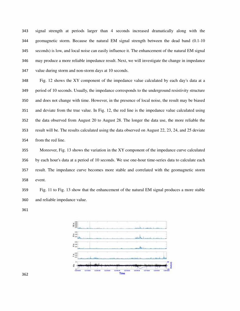
323

Fig. 9 The time-frequency distribution against the Dst index variation and the sampling rate is 15 324
Hz. The upper figure shows the time-frequency distribution from August 20 to 29. The color 325
denotes the value of 10·log10 (amp.). The lower figure shows the time variations of the Hx 326
component along with the Dst index. The unit of Hx is nT. The horizontal axis denotes the date. 327
328
329
330
Fig. 10 MT sounding curves and coherency distribution during storm days (August 26) and non-331
storm days (August 23). The black color indicates the results on the non-storm days; the red color 332
indicates the storm day results. The upper figures show the apparent resistivity. The four figures 333
at the middle layer show the impedance phase. The lower figures show the distribution of 334
coherency. The horizontal axis denotes the period in seconds. 335
336
Fig. 11 shows the amplitude variation at 16, 8, 4 and 1 second periods along with the Dst index. 337
The upper figure shows the amplitude variation from August 20 to August 28. The lower figure 338
shows the time variation of the Hx component along with the Dst index. The amplitude increased 339
at the 16, 8, and 4 seconds correlated with the geomagnetic storm. In the variation of 1 second, 340
there was no increase correlated with the storm. This result agrees that the interaction between the 341
solar wind and the magnetosphere does not contribute to the MT high-frequency signal. The 342
signal strength at periods larger than 4 seconds increased dramatically along with the 343
geomagnetic storm. Because the natural EM signal strength between the dead band (0.1-10 344
seconds) is low, and local noise can easily influence it. The enhancement of the natural EM signal 345
may produce a more reliable impedance result. Next, we will investigate the change in impedance 346
value during storm and non-storm days at 10 seconds. 347
Fig. 12 shows the XY component of the impedance value calculated by each day's data at a 348
period of 10 seconds. Usually, the impedance corresponds to the underground resistivity structure 349
and does not change with time. However, in the presence of local noise, the result may be biased 350
and deviate from the true value. In Fig. 12, the red line is the impedance value calculated using 351
the data observed from August 20 to August 28. The longer the data use, the more reliable the 352
result will be. The results calculated using the data observed on August 22, 23, 24, and 25 deviate 353
from the red line. 354
Moreover, Fig. 13 shows the variation in the XY component of the impedance curve calculated 355
by each hour's data at a period of 10 seconds. We use one-hour time-series data to calculate each 356
result. The impedance curve becomes more stable and correlated with the geomagnetic storm 357
event. 358
Fig. 11 to Fig. 13 show that the enhancement of the natural EM signal produces a more stable 359
and reliable impedance value. 360
361
362

Fig. 11 The amplitude variation in periods of 16, 8, 4 and 1 seconds against the Dst index. The 363
upper figure shows the amplitude variation from August 20 to August 28. The lowest figure 364
shows the time variation of the Hx component along with the Dst index variation. The unit of Hx 365
is nT. The horizontal axis denotes the time. 366
367
368
Fig. 12 The XY component of the impedance curve was calculated by each day's data at a period 369
of 10 seconds. The horizontal axis denotes the date. The upper figures show the apparent 370
resistivity, and the lower figures show the impedance phase. The red lines show the apparent 371
resistivity and phase calculated by the data from August 20 to August 28. 372
373
374
Fig. 13 The time variation of the impedance curves calculated using each hour's time-series data 375
at a period of 10 seconds. The horizontal axis denotes the time. One result was calculated using 376
one-hour data. The unit of Hx is nT. 377

378
Fig. 14 shows the time-frequency distribution against the Dst index. The sampling rate is 150 379
Hz, and the content is the same, as shown in Fig. 9. There were no obvious changes in the 380
intensity that were correlated with the storms in this figure. The signal strength is extremely low 381
at 50 Hz, as it is filtered out when fieldwork is carried out. On the other hand, distinct peaks 382
appeared at approximately 7.83, 14.3, 20.8 and 27.3 Hz. These frequencies correspond to the 383
frequencies of Schumann's resonances (SRs). SR is a set of spectrum peaks in the extremely low 384
frequency (ELF) of the Earth's EM field spectrum. Lightning discharges generate global EM 385
resonances in the cavity formed by the Earth's surface and the ionosphere. 386
387
388
Fig. 14 The time-frequency distribution against the Dst index. The sampling rate is 150 Hz. The 389
content is the same as Fig. 9. 390
391
4.2 Case Study 2: USArray, USA 392
In the second case study, long-period 5-component MT time-series data observed at two sites 393
(ALW48 and TNV48) were used. The data sets were recorded with a 1-second sampling period 394
for around two weeks in 2015 from the USArray project. The geomagnetic storm occurred 395
between June 22 and June 24. 396
Fig.15 shows the distribution of coherency in different periods and cross-power spectra at 16-397

second during the storm and non-storm days. The ordinary coherency increased from 4 to 40-398
second and 400 to 2,000-second during the geomagnetic storm. The low coherency during the 399
non-storm day may be attributed to the local random noise. We can see the signal strength 400
increased dramatically from the distribution of cross-power spectra. The preferred direction of PD 401
between the orthogonal electric and magnetic field becomes more obvious at 16-second. 402
Fig. 15 compared four results calculated using the data observed at site TNV48 and using 403
ALW48 as the remote reference site. The apparent resistivity of Quiet in the period from 8 to 30-404
second is severely down-biased. And the phase of Quiet is scattered from 8 to 30-second and 400 405
to 2,000-second. The result calculated using the storm data is much stable than the result 406
calculated using the non-storm data. After comparing all results, the StormRR is the most reliable, 407
and we regard it as the true model here. The Storm result is closer to the true model than the 408
Quiet result between 4 to 30-second. We can see from the case study that the signal strength 409
increased during the geomagnetic storms, and a more reliable impedance is obtained using the 410
storm data. 411
412
Fig.15 The distribution of coherency in different periods and cross-power spectra at 16-second 413
during the storm and non-storm days. The black color denotes the result using the non-storm data, 414
and the red color denotes the result using the storm data. 415

416
Fig.16 The MT sounding curves using the data observed during storm day and non-storm day. 417
The Quiet result is drawn in black; the QuietRR result is drawn in blue; the Storm result is drawn 418
in red; the StormRR result is drawn in purple. 419
420
4.3 Case Study 3: KAP03, South Africa 421
In the third case study, the long-period 5-component MT time-series data observed at Kaapvaal 422
2003 (KAP03) were used. The data were recorded with a 5-second sampling period for almost a 423
month at each site using GSC LIMS systems in 2003 as a part of the SAMTEX project. The 26 424
long-period sites distributed in a NE-SW profile are shown in the right corner of Fig. 7. Data for 425
the sites located in the middle of the profile (KAP127-KAP145) were heavily contaminated by 426
DC signals from the DC train line running between Kimberley and Johannesburg (MTNET, see 427
the website in references ). 428
Fig. 17 shows the time series at site 133. The sampling period is 5 seconds. In this dataset, 429
there was a geomagnetic storm event that was captured during the observation periods. The 430
storms lasted approximately two days, from October 29 to October 31, 2003. We used the 431
different period time-series data of the KAP03 to analyze the geomagnetic storm's influence on 432
the impedance tensor calculation. The result calculated using the data observed at quiet site 163 is 433
shown first. Then, the data observed at noisy sites 142 and 133 are analyzed in detail. Finally, the 434

results calculated using the data observed at the other site contaminated by the heavy noise 435
between sites 130 and 145 are shown. 436
437
438
Fig. 17 Time-series of MT field data at site 133. The red vertical lines show the data gaps, and the 439
black lines show the 5-component MT data. The blue line shows the variation in the Dst index. 440
The electric field unit is mV/km, and the unit of the magnetic field is nT. The horizontal axis 441
denotes the time in UTC. 442
443
Fig. 18 shows the distribution of coherency in different periods and cross-power spectra at 84 444
seconds between storm days and non-storm days at site 163. The coherency values, i.e., 445
Coh(Ex, Hy) and Coh(Ey, Hx), increased and were close to one across all periods. The preferred 446
direction of the phase difference between the orthogonal electric and magnetic fields is almost the 447
same at 84 seconds. 448
Fig. 19 shows the MT sounding curves calculated using the storm and non-storm days data at 449
site 163. The results obtained below 20 seconds are not stable. To obtain an accurate complex 450
coefficient from the time series. It is better to sample 4 points in one period. The sampling rate is 451
5 seconds. This instability may be caused by aliasing. The results calculated by EMT and BIRRP 452
using the storm and non-storm days data coincide well. From the results, we can see that the data 453

obtained during the geomagnetic storm also follows the plan-wave assumption in this area, and 454
nonstationarity is not a problem for the method based on the FFT. It will not bias the MT transfer 455
function. 456
457
458
459
Fig. 18 The distribution of coherency in different periods and cross-power spectra at 84 seconds 460
during the storm and non-storm days at site 163. 461
462
Fig. 19 The MT sounding curves calculated using the data observed during the storm and non-463
storm days at site 163. The triangles denote results calculated by the EMT code; the circles denote 464
the results calculated by the BIRRP. 465

466
Fig. 20 shows the distribution of coherency in different periods and cross-power spectra at 84 467
seconds during the storm and non-storm days at site 142. There is no preferred direction of PD 468
between the orthogonal electric and magnetic fields, and the coherency is low during the non-469
storm days. The intensity of the cross-power spectra increased almost two orders of magnitude 470
during the storm days, and the coherency increased considerably and was close to one across all 471
periods. The low coherency during the non-storm days may be attributed to the incoherent noise, 472
as shown in this case. 473
Fig. 21 shows the MT sounding curves calculated using the data observed during the storm and 474
non-storm days at site 142. The result calculated by the storm data is smoother than the Quiet and 475
QuietRR results, and the error bar is small. The QuietRR results coincide with the Storm results, 476
but the error is larger than that of the Storm results. On the other hand, the result of Quiet is quite 477
different from the results of Storm and QuietRR. Noise biased the impedance during the non-478
storm days. During the storm, the enhancement of the natural EM signal overcame the noise and 479
provided a reliable impedance. Comparing all the impedance results, Storm is the most reliable 480
from 20 to 7,00 seconds. 481
482
Fig. 20 The distribution of coherency in different periods and cross-power spectra at 84 seconds 483
during the storm and non-storm days at site 142. The red color denotes the result during storm 484

days. The black color denotes the result during non-storm days. 485
486
487
Fig. 21 MT sounding curves using the data observed during the storm and non-storm days at site 488
142. The Storm result is in red. The Quiet result is shown in black. The QuietRR result is shown 489
in blue. 490
491
Fig. 22 shows the distribution of coherency across different periods and the cross-power 492
spectra at 84 seconds during the storm and non-storm days at site 133. The values of Coh(Ex,Hy) 493
and Coh(Ey, Hx) are high during the non-storm period. However, the preferred direction of PD is 494
close to 0° and -180°. The coherent noise may have caused this phenomenon. Coherent noise 495
often appears as a spike or convex-like noise occurring simultaneously in the time domain 496
between different channels. The phase difference tends to 0° and -180°. The preferred direction of 497
PD is changed during storm days. 498
Fig. 23 shows the MT sounding curve calculated using the data observed at site 133. The XY 499
phase calculated by non-storm data is close to 0°, and the apparent resistivity increases as a line 500
on the log scale. That is the phenomenon of local noise (Zonge and Hughes, 1987). 180° or 0° 501
would correspond to a dipole electric source, which could be the train line. The impedance 502
changed using geomagnetic storm data. This result coincides with the preferred direction of PD 503
changed at 84 seconds in Fig. 22. The QuietRR result calculated using seven days of data (see 504

Table 1) coincides with the Storm result but is slightly different in the XY component between 20 505
and 40 seconds. The remote reference technique can only reduce the influence of local noise. 506
From Fig. 8, the signal strength during this storm is almost 50 times stronger than that during the 507
non-storm days. The noise can be neglected in this condition. We believe that the Storm result is 508
more reliable. 509
510
Fig. 22 The distribution of coherency across different periods and cross-power spectra at 84 511
seconds during the storm and non-storm days at site 133. The contents have the same meaning as 512
those in Fig. 20. 513
514
Fig. 23 MT sounding curves using the data observed during the storm and non-storm days at site 515
133. The contents have the same meaning as those in Fig. 21. 516

517
In this section, three parameters (polarization direction, RLcoh and R_AR) are used to analyze 518
the data observed at site 133. Fig. 24 shows the variation in the polarization direction at 84 519
seconds from October 26 to October 31. The magnetic field polarization has a preferred direction 520
at approximately -30° during non-storm days (October 26 to October 29) and becomes scattered 521
during geomagnetic storm days (October 29 to October 31). On the other hand, the electric field 522
polarization direction is scattered during non-storm days and has a preferred direction of 523
approximately 60° during geomagnetic storms. The polarization direction is a function of the 524
amplitude ratio and PD. The local EM noise source usually has a constant location; the incident 525
direction and the energy exhibit similar properties over time. Contrary to the natural EM signal, 526
the incident direction and power change with time. If there is a preferred polarization direction for 527
the magnetic field, we can consider that the local environment contaminates the data in that 528
period. That coincides with the high Coh(Ex, Hy) and Coh(Ey, Hx) and the preferred direction of 529
PD is close to 0° and -180° during the non-storm period. The data are dominated by coherent 530
noise during non-storm days. 531
Fig. 25 shows the variation in RLcoh and R_AR at 84 seconds. The data observed at site 151 532
are relatively quiet and are used as remote reference data. The blue and the red line denotes the 533
RLcoh. The blue color denotes a negative value, and the red color denotes a positive value. The 534
black curve denotes the log value of R_AR. 535
The natural magnetic signal (HMT and HrMT) comes from the same source and should be similar. 536
When the portion of the natural magnetic signal (HMT and HrMT) is high in the local and remote 537
sites; the PD will be close to 0°; therefore, RLcoh should be close to 1, and R_AR should be 538
stable and close to 1. Because the natural signal is weak and easily influenced by local noise 539
during non-storm days, RLcoh is scattered and low; R_AR is scattered and high during non-storm 540
days. The natural magnetic signal portion increased drastically during the geomagnetic storm, the 541

variation in RLcoh and R_AR became stable. This result indicates that the SNR is low during 542
non-storm days and becomes high during storm days. 543
544
545
Fig. 24 The variation in polarization direction at 84 seconds using the data observed at site 133 546
from October 26 to October 31. The upper figure shows the polarization directions for the electric 547
field, and the lower figure shows the polarization directions for the magnetic field. 548
549
Fig. 25 The variation in RLcoh versus R_AR at 84 seconds using the data observed at site 133 550
from October 26 to October 31. The blue and the red line denotes the RLcoh. Blue indicates a 551
negative value, and red indicates a positive value. The black curve denotes the log value of R_AR. 552
553
Fig. 26 shows the MT sounding curve and coherency distribution using the data observed 554
during the storm and non-storm days at site 130. The Coh(Ex, Hx) and Coh(Ey, Hx) values are high 555
between 10 and 200 seconds during the non-storm days; the XX and YX phases calculated by 556

non-storm data are close to 0°, and the apparent resistivity increases as a line on the log scale 557
between 10 and 200 seconds. A similar situation occurs at site 133. We consider that the data are 558
dominated by strong coherent noise during non-storm days. The Coh(Ex, Hx) value is high while 559
the Coh(Ex, Hy) value is low during storm days; this can be interpreted as the phenomenon of 560
PROQ. The QuietRR result using four-day data (see Table 1) coincides with the Storm result; 561
moreover, the Storm result is smoother, and the error bar is smaller than that of the QuietRR 562
result. 563
564
565
Fig. 26 The MT sounding curves and coherency distributions obtained using the data observed 566
during storm days and non-storm days at site 130. The storm result is shown in red. The quiet 567
result is shown in black. The QuietRR result is shown in blue. For coherency, the red color 568
denotes the result during storm days. The black color denotes the results obtained during non-569
storm days. 570
571
Fig. 27 shows the MT sounding curve and coherency distribution using the data observed 572
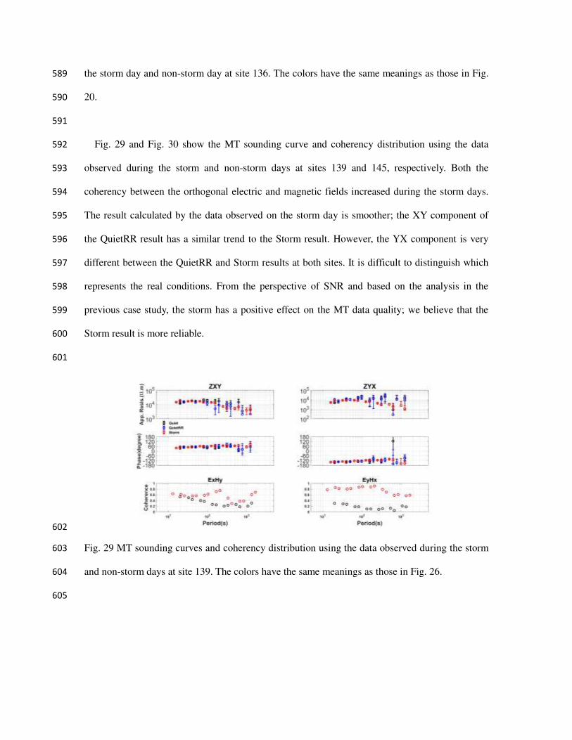
during the storm and non-storm days at site 136. Coh(Ex, Hy) is relatively high between 10 and 573
1000 seconds during the non-storm data; Fig. 28 shows the distribution of cross-power spectra of 574
the ExHx and ExHy components at 168 seconds during the storm and non-storm days. The 575

preferred direction of PD between Ex and Hy is close to 0°. We consider that the strong coherent 576
noise caused this phenomenon. 577
On the other hand, Coh(Ex, Hx) is high, while Coh(Ex, Hy) is low during the storm day. That can 578
be explained as the phenomenon of PROQ. The QuietRR result using four days of data (see Table 579
1) partially coincides with the Storm result. Moreover, the Storm result is smoother, and the error 580
bar is smaller. 581
582
583
Fig. 27 The MT sounding curves and coherency distribution using the data observed during the 584
storm and non-storm days at site 136. The colors have the same meanings as those in Fig. 26. 585
586
587
Fig. 28 Distribution of cross-power spectra of ExHx and ExHy components at 168 seconds between 588
the storm day and non-storm day at site 136. The colors have the same meanings as those in Fig. 589
20. 590
591
Fig. 29 and Fig. 30 show the MT sounding curve and coherency distribution using the data 592
observed during the storm and non-storm days at sites 139 and 145, respectively. Both the 593
coherency between the orthogonal electric and magnetic fields increased during the storm days. 594
The result calculated by the data observed on the storm day is smoother; the XY component of 595
the QuietRR result has a similar trend to the Storm result. However, the YX component is very 596
different between the QuietRR and Storm results at both sites. It is difficult to distinguish which 597
represents the real conditions. From the perspective of SNR and based on the analysis in the 598
previous case study, the storm has a positive effect on the MT data quality; we believe that the 599
Storm result is more reliable. 600
601
602
Fig. 29 MT sounding curves and coherency distribution using the data observed during the storm 603
and non-storm days at site 139. The colors have the same meanings as those in Fig. 26. 604
605

606
Fig. 30 MT sounding curves and coherency distribution using the data observed during the storm 607
and non-storm days at site 145. The colors have the same meanings as those in Fig. 26. 608
609
5 DISCUSSION 610
In this section, we discuss how to use multiple parameters to estimate the data quality. Coherency 611
is an important parameter to discuss the data quality. However, the characteristic of coherency is 612
different in different situations. At first, we discuss the relationship between impedance and 613
coherency. According to least-squares theory (Sims et al., 1971); Zxy can be calculated as follows: 614
Zxy = <ExH̅y><HxH̅x> − <ExH̅x><HxH̅y><HyH̅y><HxH̅x> − <HyH̅x><HxH̅y> = C − DE− F, (14) 615
For the denominator, there is a relationship between the coherency as follows: 616
|C|=|< ExH̅y >< HxH̅x >|= coh(Ex, Hy) √< ExE̅x >< HyH̅y > < HxH̅x > , (15) 617
|D|=|< ExH̅x >< HxH̅y >|= coh(Ex, Hx) √< ExE̅x >< HxH̅x > coh(Ex, Hx) √< HxH̅x >< HyH̅y > , (16) 618
|𝐶||D|=|<ExH̅y><HxH̅x>||<ExH̅x><HxH̅y>| = coh(Ex,Hy)coh(Ex,Hx)coh(Hx,Hy) , (17) 619
For the denominator part of equation 14, there is a relationship as follows: 620
|E| = |< HxH̅x >< HyH̅y >| (18) 621
|F| = |< HyH̅x >< HxH̅y >| = coh2(Hx, Hy) < HxH̅x >< HyH̅y > (19) 622

|𝐸||F| = 1coh2(Hx,Hy) (20) 623
Because various sources generate natural magnetic signals, they generate magnetic fields that 624
vary in their incident directions, which means Hx and Hy are not coherent, and Coh(Hx, Hy) is a 625
small value. In the condition that the Coh(Ex, Hy) is relatively high while the Coh(Ex, Hx) is small. 626
The numerator of Eq. 14 will be dominant by the C part. The denominator is dominant by the E 627
part. 628
The Zxy can be rewritten as follows: 629
Zxy = <ExHy†><HyHy†> . (21) 630
In this situation, Zxy is determined by the orthogonal component of the electric and magnetic field. 631
A similar analysis to Zxx , Zxx is undeterminable. When Coh(Ex, Hy ) is relatively high while 632
Coh(Ex, Hx) is small; the field data can be explained as the 1-D and 2-D cases. Here we also need 633
to quantify the coherency value in the different geological environments by doing some 634
simulation. For example, rotate the observation axes in the 2-D case by the step of 5°, how high 635
the coherency will be. We can see the example at TNV 48 from USArray, site 142 from KAP03. 636
The coherency between the orthogonal magnetic and electric components is relatively low during 637
the non-storm day and increased dramatically during the strong storm. The low coherency can be 638
attributed to the incoherent noise in this case. 639
On the contrary that the coherency between the orthogonal component Coh(Ex, Hy) is relatively 640
low while the Coh( Ex, Hx ) is high. The Zxy is undeterminable and Zxx is determinable. The 641
phenomenon of PROQ appears. In this situation, we cannot explain the data by the 1-D or 2-D 642
case. We can see the example at Sawauchi station, sites 130 and 136 from KAP03. Both site 130 643
and 136 is contaminated by coherent noise, and the Coh(Ex, Hy) become low while the Coh(Ex, Hx) 644
become relatively high during the storm day. 645
The coherent noise may have a high coherency value and appear as the spike, or convex-like, 646
or other kinds of noise in the time domain at the different channel simultaneously. And the phase 647
difference between the two-channel tends to 0° or 180°. It is better to check the phase by plot the 648
distribution of the cross-power spectra. To estimate the data quality precisely, we would better 649
combine other parameters to discuss the situation. 650
The polarization direction is a function of PD and AR between the two orthogonal fields. The 651
local EM noise source usually has a constant location; the incident direction and the energy have 652
a similar property along with time. Contrary to the natural EM signal, the incident direction and 653
power are changed with time. If there is a preferred polarization direction for the magnetic field, 654
we can consider that the data is contaminated by coherent noise in that period. This situation can 655
be seen at site 133. But sometimes, the data is contaminated by incoherent noise. There is no 656
preferred polarization direction for the magnetic field. This situation appears in site 142 but is not 657
shown in this paper. 658
Suppose there is a quiet remote reference site. We also could use the RLcoh and R_AR to 659
measure the similarity between the local and remote sites to evaluate the influence of noise. This 660
example is shown in the data analysis at site 133. 661
Finally, the most important parameter to discuss the data quilty is the result impedance. The 662
sounding curve should be smooth according to the forwarding modeling. On the other hand, in 663
the influence of strong locale noise, the phase will be close to 0º or 180°, and the apparent 664
resistivity increases as a line in the log scale (Zonge and Hughes, 1987); this phenomenon appear 665
during the non-storm day at site 130 and 133. Because the remote reference technique can 666
suppress the local noise, and the remote reference result can be used as a standard to evaluate the 667
data quality. The examples are shown in sites 130,136,139,145 from KAP03 and TNV48 from 668
USArray. Until now, we discussed how to use multiple parameters to estimate the geomagnetic 669
storm on the data quality. All examples of the method can be found in the case studies. 670
Finally, we will discuss the source effect and nonstationarity of the data observed during the 671
storm day. At mid-latitudes, geomagnetic pulsations (Pc's) in the Pc3-4 band (~10 - 100 s) 672
associated with field-line resonances can violate the fundamental assumption of the MT method 673
over the resistive regions; where skin depths are large (Murphy and Egbert, 2018). In this case, 674
the source effect is inevitable and is place-dependent. In this paper, from the perspective of SNR, 675
we demonstrate the positive effect of a geomagnetic storm on the MT data quality, the impedance 676
calculated using the data observed during the geomagnetic storm and the non-storm day at the 677
quiet site 163 and Sawauchi station coincide well. It shows that the signal holds the plane-wave 678
assumption, and the nonstationarity is not a problem for the method based on the FFT in this area. 679
Otherwise, the result calculated by the storm period data should be biased. The souces effect may 680
be considered near the auroral or equatorial electrojets. But the plane wave assumption is 681
generally acceptable at midlatitudes. 682
683
6 CONCLUSIONS 684
It is well known that the signal strength will increase during a geomagnetic storm in the MT 685
community. Still, the demonstration that shows the positive effects on the MT impedance by the 686
field data is rare. This paper showed the positive influence of the geomagnetic storm on MT data 687
quality by three case studies in mid-latitude. Using the data observed during a strong geomagnetic 688
storm may overcome the influence of the local noise, depending on the strength of the 689
geomagnetic storm and local noise. We obtained a more reliable and interpretable impedance 690
using the data observed during the strong geomagnetic storm to calculate the impedance in the 691
survey line from Kap03, which is contaminated by the strong noise. 692
MT field data include natural signal sources and noise. Along with urban constructions, 693
artificial disturbances to EM observations are becoming more and more serious. The observation 694
occasionally contains continuous noise, which is difficult to get a reliable result from the current 695
technique. When we redo the MT campaign in the noisy site, we may get a reliable result using 696
the data observed during geomagnetic storms. Sometimes, the variation during storm periods can 697
be 100 times greater than in the non-storm period data. In that condition, the noise can be 698

neglected. However, a strong geomagnetic storm doesn't occur frequently. It is possible to predict 699
the geomagnetic storm by the space weather forecast information. The Space Weather Prediction 700
Center (SWPC; see the website in references) provides information about space weather in the 701
coming three days. Utilizing the data observed during the strong geomagnetic storm may bring a 702
reliable result despite the site contaminated by continuous noise. 703
To get the accurate complex coefficient from the time series, we suggest that it is better to 704
contain at least four times longer than the expected period. For 1,000-second, a time-series 705
segment with 4,000 seconds is needed to get accurate spectra. The overlay rate is 50% to keep 706
each data's independence and get more sample data. By the continuous 4-hour time-series data, 707
we may get about eight samples to do the impedance estimation in the frequency domain by FFT. 708
If there is continuous 4-hour geomagnetic storm data, we may get a relatively reliable tensor until 709
1,000 seconds, depending on the geomagnetic storm's length. The longer the geomagnetic storm 710
last. A more stable result can be obtained. By the statistical analysis of the geomagnetic storm, 711
one year had about ten strong geomagnetic events, and about five events lasted more than 4 hours 712
on average. That is practical and meaningful for MT exploration. 713
714
DECLARATION 715
716
Availability of data and materials 717
The magnetic time-series data observed at the KAK station is downloaded from the 718
INTERMAGNET ( International Real-time Magnetic Observatory Network). The SAMTEX team 719
and USArray team provided the long period time-series data to investigate. Kap03 data can be 720
download from MTNET (see the reference). USArray data can be download from IRIS 721
(Incorporated Research Institutions for Seismology). Nittetsu Mining Consultants Co., Ltd. 722
provided the broadband frequency MT time-series data observed at Sawauchi, Japan. The Dst 723
index data can be download from the WDC for Geomagnetism, Kyoto. Alan Chave provided the 724

BIRRP code. Maik Neukirch provided the EMT code. 725
726
Competing interests 727
We know of no conflicts of interest associated with this publication. We declare that this 728
manuscript is original, has not been published before and is not currently being considered for 729
publication elsewhere. 730
731
Funding 732
'Not applicable.' 733
734
Authors' contributions 735
Hao Chen processed the time series data, created the result and wrote the paper. Hao Chen 736
contributes about 60%. Hideki Mizunaga reviewed the paper and contributed about 30%; 737
Toshiaki Tanaka contributed about 10% to this work. 738
739
Acknowledgments 740
We thank the INTERMAGNET (International Real-time Magnetic Observatory Network) for 741
providing the magnetic time-series data observed at the KAK station. We thank all SAMTEX and 742
USArray team members for providing the time-series data used in this study. We also thank 743
Nittetsu Mining Consultants Co., Ltd. for providing the broadband frequency MT time-series data 744
observed at Sawauchi, Japan. We thank the WDC for Geomagnetism, Kyoto, for providing the 745
Dst index data to do the statistical analysis of the geomagnetic storm. Finally, we express special 746
thanks to Maik Neukirch for his constructive comments to improve the manuscript. We also 747
thank Ute Weckmann, Louise Alexander, Ben Murphy, James Macnae and two anonymous 748
reviewers who reviewed and gave us constructive comments to improve the manuscript. 749
750

REFERENCES 751
Cagniard, L., 1953. The basic theory of the magneto-telluric method of geophysical prospecting. 752
Geophysics, 18, 605–635. 753
Constable, C., 2016. Earth's electromagnetic environment. Surv, Geophysics, 37, 27–45. 754
Constable, C. G. and Constable, S.C., 2004. Satellite magnetic field measurements: applications 755
in studying the deep Earth. State Planet Front. Chall. Geophysics, 19, 147. 756
Chen, J., Heincke, B., Jegen, M. and Moorkamp, M. 2012. Using empirical mode decomposition 757
to process marine magnetotelluric data, Geophys. J. Int., 190, 293–309. 758
Chouteau, MTournerie, B., 2000. Analysis of magnetotelluric data showing phase rolling out of 759
quadrant (PROQ), SEG Technical Program Expanded Abstracts 2000. Society of Exploration 760
Geophysicists, pp. 344–346. 761
Chave, A. D. and Thomson, D. J., 2004. Bounded influence estimation of magnetotelluric 762
response functions, Geophys. J. Int, 157, 988–1006. 763
Chave, A.D., Jones, A.G., 2012. The magnetotelluric method: Theory and practice. Cambridge 764
University Press. 765
Egbert, G.D., Eisel, M., Boyd, O.S., Morrison, H.F., 2000. DC trains and Pc3s: Source effects in 766
mid‐latitude geomagnetic transfer functions. Geophys. Res. Lett. 27, 25–28. 767
Fowler, R.A., Kotick, B.J., Elliott, R.D., 1967. Polarization analysis of natural and artificially 768
induced geomagnetic micropulsations. J. Geophys. Res. 72, 2871–2883. 769
Gamble, T. D., Goubau, W. M. and Clarke, J., 1979. Magnetotellurics with a remote reference, 770
Geophysics, 44, 53–68. 771
Garcia, X., Chave, A.D., Jones, A.G., 1997. Robust processing of magnetotelluric data from the 772
auroral zone. J. Geomagn. Geoelectr. 49, 1451–1468. 773
Garcia, X. and Jones, A. G., 2002. Atmospheric sources for audio-magnetotelluric (AMT) 774
sounding, Geophysics, 67, 448-458. 775

Hennessy, L., Macnae, J., 2018. Source-dependent bias of sferics in magnetotelluric responses. 776
Geophysics 83, E161–E171. 777
Lezaeta, P., Chave, A., Jones, A.G., Evans, R., 2007. Source field effects in the auroral zone: 778
Evidence from the Slave craton (NW Canada). Phys. Earth Planet. Inter. 164, 21–35. 779
Marple, S.L., Marino, C., 2004. Coherency in signal processing: a fundamental redefinition, 780
Conference Record of the Thirty-Eighth Asilomar Conference on Signals, Systems and 781
Computers, 2004. IEEE, pp. 1035–1038. 782
Murphy, B.S., Egbert, G.D., 2018. Source biases in midlatitude magnetotelluric transfer functions 783
due to Pc3-4 geomagnetic pulsations. Earth Planets Space 70, 1–9. 784
McPherron, R.L., 2005. Magnetic pulsations: their sources and relation to solar wind and 785
geomagnetic activity, Surv. Geophysics, 26, 545–592. 786
Mareschal, M., 1981. Source effects and the interpretation of geomagnetic sounding data at sub-787
auroral latitudes. Geophys. J. Int. 67, 125–136. 788
MTNET, https://www.MTnet.info/data/kap03/kap03.html. 789
Neukirch, M. and Garcia, X. 2014. Nonstationary magnetotelluric data processing with the 790
instantaneous parameter, J. Geophys. Res. Solid Earth, 119, 1634–1654. 791
Oettinger, G., Haak, V., Larsen, J. C., 2001. Noise reduction in magnetotelluric time-series with a 792
new signal–noise separation method and its application to a field experiment in the Saxonian 793
Granulite Massif, Geophys. J. Int, 146, 659–669. 794
Rikitake, T., 1948. 1. Notes on electromagnetic induction within the Earth. Bull. Earthquake Res. 795
Inst., 24, 1-9. 796
Sims, W. E., Bostick, F. X., and Smith, H. W., 1971. The estimation of magnetotelluric impedance 797
tensor elements from measured data, Geophysics, 36, 938–942. 798
Smirnov, M. Y., 2003. Magnetotelluric data processing with a robust statistical procedure having 799
a high breakdown point, Geophys. J. Int., 152, 1–7. 800
SWPC (The Space Weather Prediction Center), 801

https://www.swpc.noaa.gov/content/wmo/geomagnetic-activity. 802
Tikhonov, A. N., 1950. On determining electrical characteristics of the deep layers of the Earth's 803
crust, in Doklady, Citeseer, 295–297. 804
Viljanen, A., Pirjola, R., & Hákkinen, L., 1993. An attempt to reduce induction source effects at 805
high latitudes, Journal of geomagnetism and geoelectricity, 45(9), 817-831. 806
Weckmann, U., Magunia, A. and Ritter, O., 2005. Effective noise separation for magnetotelluric 807
single site data processing using a frequency domain selection scheme, Geophys. J. Int., 161, 808
635–652. 809
Weckmann, U., Ritter, O., Haak, V., 2003. A magnetotelluric study of the Damara Belt in Namibia: 810
2. MT phases over 90 reveal the internal structure of the Waterberg Fault/Omaruru Lineament. 811
Phys. Earth Planet. Inter. 138, 91–112. 812
Yu, G., Xiao, Q., Li, M., 2018. Anisotropic Model Study for the Phase Roll Out of Quadrant Data 813
in Magnetotellurics. 814
Zonge, K. L. and Hughes, L. J., 1987. Controlled source audio-frequency magnetotellurics, in 815
Electromagnetic Methods in Applied Geophysics. Applications (ed. Nabighian, M. N.), SEG, 816
713–809. 817
818

Figures
Figure 1
The geomagnetic intensities along the N-S direction during a storm day and a non-storm day. The blacklines denote the non-storm day's data, and the red lines denote the storm day's data. The left is a pro�le inthe time domain, and the right is a pro�le in the frequency domain.
Figure 2
The distribution of strong storms based on the Dst index between 1957 - 2020, the orange line denotesDst (<= -50 nT), and the light blue line denotes Dst (<= -100 nT).

Figure 3
The statistical analysis of each strong geomagnetic storm event. The upper �gure shows the number ofeach strong geomagnetic storm event in a different storm event length. The lower �gure shows thecumulative distribution of the upper �gure.
Figure 4
The monthly count of strong geomagnetic storms based on the Dst index.

Figure 5
The yearly count of geomagnetic storms based on the Dst index from 1957 to 2020.
Figure 6
The calculated periods by Fourier analysis using the yearly count of geomagnetic storms from 1957 to2020.

Figure 7
The location map in the three case studies (KAP03, USArray, Sawauchi). The left map shows the detailedsite location used in USArray, and the right map shows the survey line of KAP03. Note: The designationsemployed and the presentation of the material on this map do not imply the expression of any opinionwhatsoever on the part of Research Square concerning the legal status of any country, territory, city orarea or of its authorities, or concerning the delimitation of its frontiers or boundaries. This map has beenprovided by the authors.
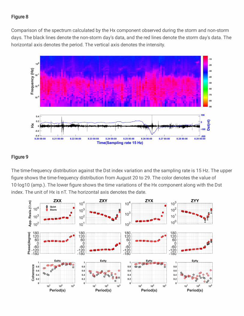
Figure 8
Comparison of the spectrum calculated by the Hx component observed during the storm and non-stormdays. The black lines denote the non-storm day's data, and the red lines denote the storm day's data. Thehorizontal axis denotes the period. The vertical axis denotes the intensity.
Figure 9
The time-frequency distribution against the Dst index variation and the sampling rate is 15 Hz. The upper�gure shows the time-frequency distribution from August 20 to 29. The color denotes the value of10·log10 (amp.). The lower �gure shows the time variations of the Hx component along with the Dstindex. The unit of Hx is nT. The horizontal axis denotes the date.
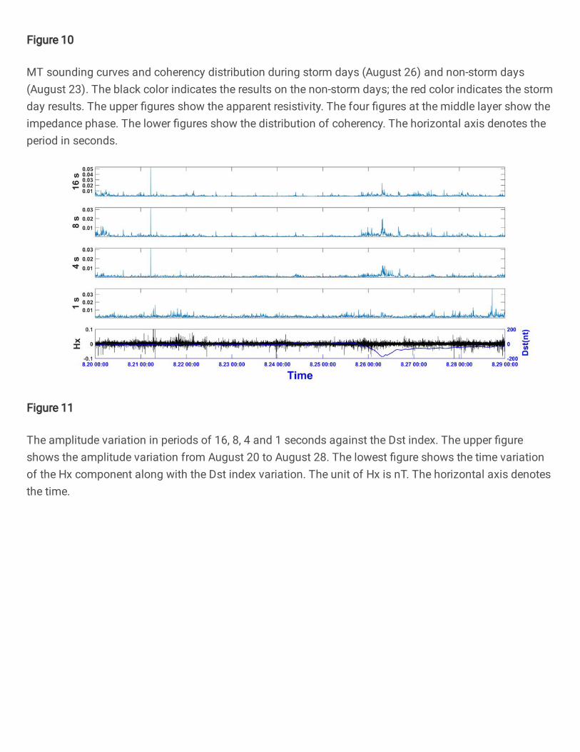
Figure 10
MT sounding curves and coherency distribution during storm days (August 26) and non-storm days(August 23). The black color indicates the results on the non-storm days; the red color indicates the stormday results. The upper �gures show the apparent resistivity. The four �gures at the middle layer show theimpedance phase. The lower �gures show the distribution of coherency. The horizontal axis denotes theperiod in seconds.
Figure 11
The amplitude variation in periods of 16, 8, 4 and 1 seconds against the Dst index. The upper �gureshows the amplitude variation from August 20 to August 28. The lowest �gure shows the time variationof the Hx component along with the Dst index variation. The unit of Hx is nT. The horizontal axis denotesthe time.

Figure 12
The XY component of the impedance curve was calculated by each day's data at a period of 10 seconds.The horizontal axis denotes the date. The upper �gures show the apparent resistivity, and the lower�gures show the impedance phase. The red lines show the apparent resistivity and phase calculated bythe data from August 20 to August 28.
Figure 13
The time variation of the impedance curves calculated using each hour's time-series data at a period of10 seconds. The horizontal axis denotes the time. One result was calculated using one-hour data. Theunit of Hx is nT.

Figure 14
The time-frequency distribution against the Dst index. The sampling rate is 150 Hz. The content is thesame as Fig. 9.

Figure 15
The distribution of coherency in different periods and cross-power spectra at 16-second during the stormand non-storm days. The black color denotes the result using the non-storm data, and the red colordenotes the result using the storm data.

Figure 16
The MT sounding curves using the data observed during storm day and non-storm day. The Quiet resultis drawn in black; the QuietRR result is drawn in blue; the Storm result is drawn in red; the StormRR resultis drawn in purple.
Figure 17
Time-series of MT �eld data at site 133. The red vertical lines show the data gaps, and the black linesshow the 5-component MT data. The blue line shows the variation in the Dst index. The electric �eld unitis mV/km, and the unit of the magnetic �eld is nT. The horizontal axis denotes the time in UTC.

Figure 18
The distribution of coherency in different periods and cross-power spectra at 84 seconds during the stormand non-storm days at site 163.

Figure 19
The MT sounding curves calculated using the data observed during the storm and non-storm days at site163. The triangles denote results calculated by the EMT code; the circles denote the results calculated bythe BIRRP.

Figure 20
The distribution of coherency in different periods and cross-power spectra at 84 seconds during the stormand non-storm days at site 142. The red color denotes the result during storm days. The black colordenotes the result during non-storm days.

Figure 21
MT sounding curves using the data observed during the storm and non-storm days at site 142. The Stormresult is in red. The Quiet result is shown in black. The QuietRR result is shown in blue.

Figure 22
The distribution of coherency across different periods and cross-power spectra at 84 seconds during thestorm and non-storm days at site 133. The contents have the same meaning as those in Fig. 20.

Figure 23
MT sounding curves using the data observed during the storm and non-storm days at site 133. Thecontents have the same meaning as those in Fig. 21.
Figure 24
The variation in polarization direction at 84 seconds using the data observed at site 133 from October 26to October 31. The upper �gure shows the polarization directions for the electric �eld, and the lower �gureshows the polarization directions for the magnetic �eld.

Figure 25
The variation in RLcoh versus R_AR at 84 seconds using the data observed at site 133 from October 26 toOctober 31. The blue and the red line denotes the RLcoh. Blue indicates a negative value, and redindicates a positive value. The black curve denotes the log value of R_AR.
Figure 26
The MT sounding curves and coherency distributions obtained using the data observed during stormdays and non-storm days at site 130. The storm result is shown in red. The quiet result is shown in black.The QuietRR result is shown in blue. For coherency, the red color denotes the result during storm days.The black color denotes the results obtained during non-storm days.

Figure 27
The MT sounding curves and coherency distribution using the data observed during the storm and non-storm days at site 136. The colors have the same meanings as those in Fig. 26.

Figure 28
Distribution of cross-power spectra of ExHx and ExHy components at 168 seconds between the stormday and non-storm day at site 136. The colors have the same meanings as those in Fig. 20.

Figure 29
MT sounding curves and coherency distribution using the data observed during the storm and non-stormdays at site 139. The colors have the same meanings as those in Fig. 26.
Figure 30
MT sounding curves and coherency distribution using the data observed during the storm and non-stormdays at site 145. The colors have the same meanings as those in Fig. 26.
Supplementary Files

This is a list of supplementary �les associated with this preprint. Click to download.
StormVSnon.jpg