Embed Size (px)
Citation preview

The Influence of Demographics and Household Specific Price Indices
on
Expenditure Based Inequality and Welfare:
A Comparison of Spain and the United States
BY
Thesia I. Garner1, Javier Ruiz-Castillo2, and Mercedes Sastre Garcia3
Prepared for the Southern Economics Association Annual Conference
Atlanta, Georgia 21-23 November 1997
Discussant: John P. Formby, University of Alabama
1Garner's address: Division of Price and Index Number Research, U.S. Bureau of Labor Statistics, Postal Square Building, Room 3105, 2 Mass. Ave., N. E., Washington, D. C. 20212; telephone: (202)606-6579 extension 596; fax: (202)606-6583; email: [email protected]'s address: Departamento de Economic, Universidad Carlos III, 28903-Getafe, Spain; telephone: [+34+1] 624 9588; fax: [+34+1] 624 9329; email: [email protected] 3Sastre Garcia's address: Departamento de Economic Aplicada VI, Universidad Complutense de Madrid, Campus de Somosaguas, 28223 Madrid, Spain; email: [email protected]
For their comments, the authors would like to thank Jorge Salazar-Carillo, Michael Wolfson, and other participants in the Session on International Comparisons of Income and Wealth Statistics during the 51st Session of the International Statistical Institute (August 1997). A tremendous thanks is extended to Rob Cage of the BLS who produced the indexes for the U.S. and the primary data set used for the analysis. All views expressed in this paper are those of the authors and do not reflect the views or policies of the Bureau of Labor Statistics (BLS) or other BLS staff members, the Universidad Carlos III, or the Universidad Complutense de Madrid. The responsibility for errors remains with the authors.
ABSTRACT
The purpose of this research is to examine the role of household size and household specific price indices on inequality and welfare measurement in Spain and the U.S. Total household expenditures from each countries' 1990-91 consumer expenditure surveys are used for the analysis. Decomposable measurement instruments are used both for the inequality and social welfare analyses. Thus we can isolate the impact of household size on inequality, separating this affect from the distributional impact due to between group differences in inequality. For different time periods, we examine the impact of changes in relative prices on both inequality and welfare. To test the sensitivity of our overall results, different household size scale factors are applied to total expenditures to produce adjusted expenditures. The household specific price indices are used to express the 199091 expenditure distributions at winter of 1981 and winter of 1991 prices. Diary data are employed to allocate Diary specific commodities to Interview households in the U.S. case. Our results show that wide differences in demographic factors can be very important in international comparisons. Inequality and welfare comparisons are drastically different for smaller and larger households. Given this diversity, decomposable measurement instruments help to explain how results at the household size level get translated at the population level. In terms of the influence of relative prices on inequality, for both countries, we find that from the point of view of winter 1981; the amount of expenditures that we would need to give to richer households to compensate them for inflation, over the 1981 to 1991 period, would be greater than the amount that we would need to give to poorer households for them to remain at the same level of welfare. However, because the distributional impact of relative prices is of a comparable order of magnitude, our inequality comparisons are rather robust to the choice of the reference price vector. KEYWORDS: Theil Inequality; Welfare; Household Expenditures; Household Specific Price Indexes

1. INTRODUCTION
In this paper we compare levels of living in Spain and the United States (U.S.)
using current household consumption expenditures as our level of living measure. As in
most welfare analysis, we assume that social or aggregate welfare can be expressed in
terms of two statistics of the expenditure distribution: the mean and an index of relative
inequality.
Like intertemporal comparisons of income inequality and welfare in a single
country, international comparisons of expenditures require the solution to the following
four classical problems: (a) how to make comparable two heterogeneous populations
consisting of households with different needs; (b) which measurement instruments to
use among the admissible inequality measures; (c) which measurement instruments to
use among the admissible welfare measures, and (d) how to make comparable the
money distributions in both countries.
To solve the difficulties arising from the demographic heterogeneity in
international comparisons, researchers usually compare the distributions of equivalent
expenditures (or equivalent income) using some common equivalence scale.1 However,
as Coulter et al. (1992a) conclude in their review of the literature, there is no single
'correct' equivalence scale for adjusting incomes. Thus, a range of scale relativities is
both justifiable and inevitable. In this paper, to make the analysis tractable we assume
that equivalence scales depend only on the number of persons in the household.
Following Buhmann et al. (1988) and Coulter et al. (1992a, 1992b), to pool all
households into a unique distribution within each country we use a parametric model of
equivalence scales which allows for different views about the importance of economies
of scale in consumption within the household. 2 1
See Phipps and Garner (1994) and Burkhauser et al. (1996). 2
For the use in this model in international comparisons, see also Atkinson et al. (1995).
2

In the equivalence scales model, expenditures for households of the same size
are directly comparable. Thus, we believe it is important to start our analysis from
inequality (or welfare) comparisons separately for each of subgroups in the partition by
household size. Then, in order to go from the household size to the population level, we
find illuminating to work with additively decomposable measurement instruments. For
every population partition, decomposable measures of (relative) inequality allow us to
express overall inequality in a cross-section as the sum of two terms: a weighted sum of
within-group inequalities, plus a between-group inequality component calculated as if
each person within a given group received the group's mean income.
Using decomposable measures, in this paper we explain the overall inequality
differences between the U.S. and Spain in terms of three factors: i) the difference in
within-group inequality (due to differences in subgroup inequality values), ii) the
difference in between-group inequality (due to the relative differences in subgroup
means), and iii) the demographic change across partition subgroups (due to differences
in subgroup population shares). In addition, following a suggestion in Coulter et al
(1992a) and developed in Del Rio and Ruiz-Castillo (1997b), we use a method to free
the decomposition analysis from the possible ‘contamination’ that will arise if we use an
inappropriate equivalence scale.
As far as the measurement of welfare is concerned, we are interested in social
evaluation functions (SEF for short) which permit the explanation of welfare
differences in terms of differences in the mean and differences in relative inequality. As
in the inequality case, additively decomposable SEFs have been found useful in
intertemporal welfare comparisons within a single country.3 In this paper we show that
these methods are equally useful in international comparisons. This is important in a
context in which we find considerable welfare and demographic inter-country
differences between the subgroups in the partition by household size. 3See Ruiz-Castillo (1998).
3
We address each of these issues using data from household budget surveys. The
Spanish data are from the Encuesta de Presupuestos Familiares (EPF) conducted by the
Instituto Nacional de Estadistica (INE), and the U.S. data are from the Consumer
Expenditure Survey (CEX) from the Bureau of Labor Statistics (BLS). We compare
annual consumer unit (referred to here as household) expenditures, which were
collected by the agencies from April 1990 through March 1991 for Spain and from
January 1990 through December 1991 for the U.S. We refer to this time period as
1990-91. We express both distributions at constant prices for two periods in each
country: the winter of 1991 and the winter of 1981. Since we use household specific
price indices, we are able to take into account the distributional role of changes in price
relatives during the 1980's in both countries. Finally, we express the Spanish
distributions in U.S dollars using EKS Purchasing Power Parities (Godbout 1997;
OCED 1993).
The comparison between Spain and the U.S. is an interesting one. First, Spain has
been experiencing a complex process of economic modernization and liberalization since
the mid-1970's, including full membership into the European Union in January 1986,
resulting in a more open and market oriented economy. In contrast, the U.S.- has a much
larger economic system which is rather open and market oriented. Second, during this
period Spain has been taking important steps toward a fairly comprehensive social safety
net, in the European style, while that of the U.S. is rather limited. Third, tax structures
are rather different too. Although a modern income tax system did not start in Spain until
1978, it is more progressive today than is the U.S. tax system. On the other hand, the EU
membership lead to the introduction in 1986 of a value added tax in Spain, in contrast to
the indirect tax system in the U.S. Fourth, recent trends in inequality and welfare are
quite different. In particular, from 1973-74 to 1990-91, expenditure inequality has fallen
in Spain (Del Rio and Ruiz-Castillo 1997a, 1997b; Ruiz-Castillo 1995b), but has
increased during the 1980's in the U.S. (for example, see Johnson and Shipp 1997). And

fifth, the demographic structure of the two countries is very different, with
larger consuming units in Spain on average than in the U.S.
The remainder of this paper is organized into four sections. Section two presents
the methods and Section three, a description of the data. Section four includes our results
and Section five summaries and concludes.
II. METHODS A. Interpersonal Comparisons of Welfare
Assume we have a population of h = 1,...,H households whose living standards
can be adequately represented by a one-dimensional variable we call income, xh.
Households can differ in income and/or a vector of household characteristics. As
indicated in the Introduction, we assume that equivalence scales depend only on the
number of persons in the household. Households of the same size are assumed to have
the same needs and, therefore, their incomes are directly comparable. Larger households
have greater needs, but also greater opportunities to achieve economies of scale in
consumption. Assume that there are m = 1,...,M household sizes. Following Buhmann et
al. (1988) and Coulter et al. (1992a, 1992b), for each household h of size m we define
adjusted income by
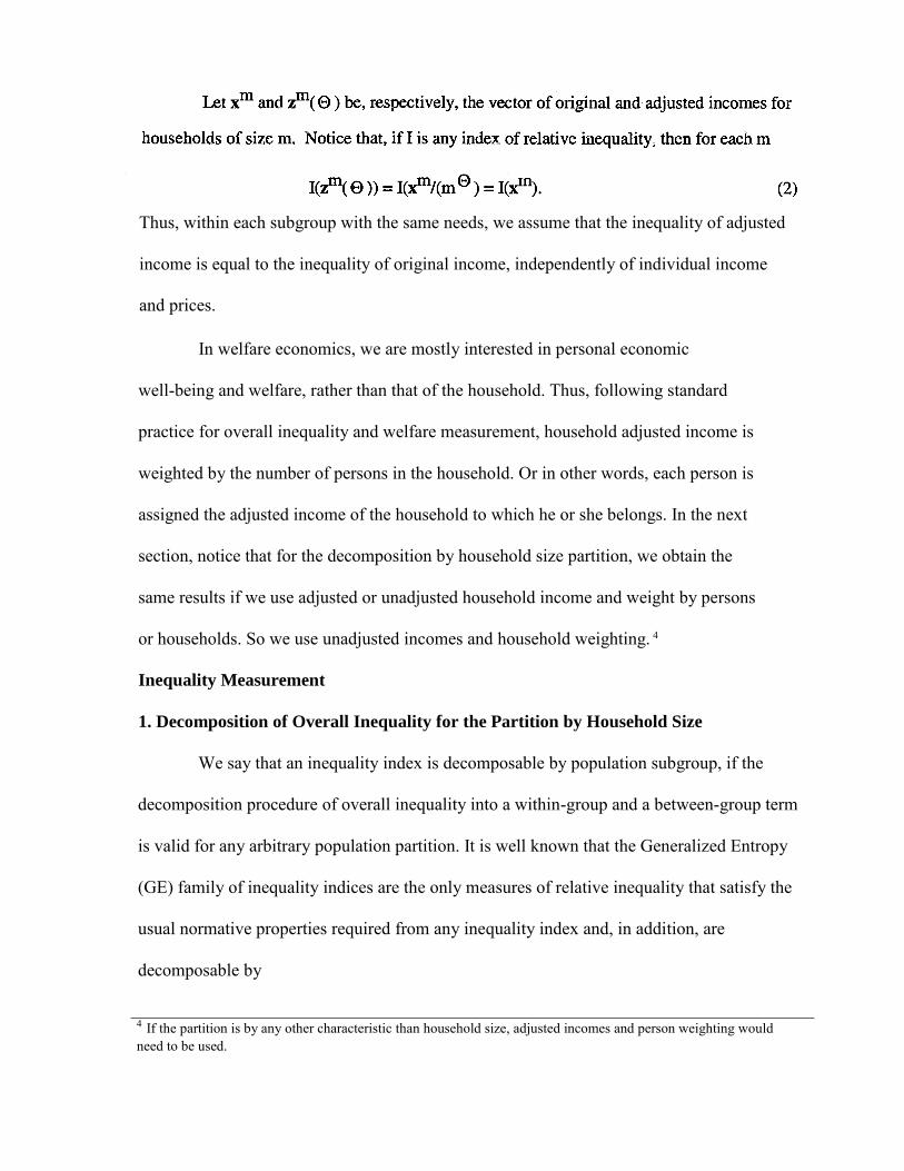
Thus, within each subgroup with the same needs, we assume that the inequality of adjusted
income is equal to the inequality of original income, independently of individual income
and prices.
In welfare economics, we are mostly interested in personal economic
well-being and welfare, rather than that of the household. Thus, following standard
practice for overall inequality and welfare measurement, household adjusted income is
weighted by the number of persons in the household. Or in other words, each person is
assigned the adjusted income of the household to which he or she belongs. In the next
section, notice that for the decomposition by household size partition, we obtain the
same results if we use adjusted or unadjusted household income and weight by persons
or households. So we use unadjusted incomes and household weighting. 4
Inequality Measurement
1. Decomposition of Overall Inequality for the Partition by Household Size
We say that an inequality index is decomposable by population subgroup, if the
decomposition procedure of overall inequality into a within-group and a between-group term
is valid for any arbitrary population partition. It is well known that the Generalized Entropy
(GE) family of inequality indices are the only measures of relative inequality that satisfy the
usual normative properties required from any inequality index and, in addition, are
decomposable by 4 If the partition is by any other characteristic than household size, adjusted incomes and person weighting would need to be used.
6
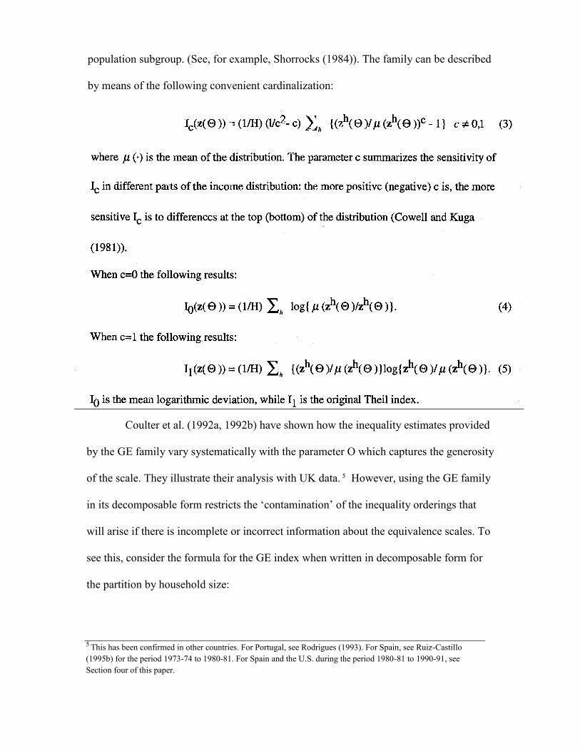
population subgroup. (See, for example, Shorrocks (1984)). The family can be described
by means of the following convenient cardinalization:
Coulter et al. (1992a, 1992b) have shown how the inequality estimates provided
by the GE family vary systematically with the parameter O which captures the generosity
of the scale. They illustrate their analysis with UK data. 5 However, using the GE family
in its decomposable form restricts the ‘contamination’ of the inequality orderings that
will arise if there is incomplete or incorrect information about the equivalence scales. To
see this, consider the formula for the GE index when written in decomposable form for
the partition by household size:
5 This has been confirmed in other countries. For Portugal, see Rodrigues (1993). For Spain, see Ruiz-Castillo (1995b) for the period 1973-74 to 1980-81. For Spain and the U.S. during the period 1980-81 to 1990-91, see Section four of this paper.
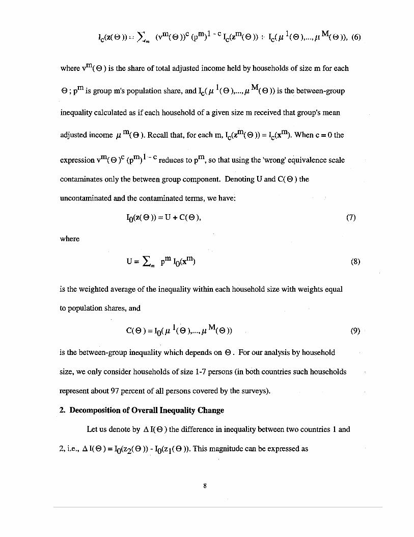

Equation (11) is the difference in uncontaminated inequality, which is seen to be the
sum of two terms: equation (12), which is the weighted sum of inequality differences
within each household size, and equation (13) which captures the impact on the
uncontaminated inequality of demographic differences across the partition by household
size. Both are independent of , which only affects equation (14), namely, the
difference in between-group inequality in the partition by household size.
Of course, demographic shares for country 2, rather than for country 1, and
the inequality for country I can be used in the above decomposition. In this case, we
have:
C. Welfare Measurement
1. Admissible Social Evaluation Functions
9

But which SEFs within these classes should we use in applied work? The following
property leads us to an appropriate selection.
Suppose that we have two islands where income is equally distributed but whose
means are different. If they now form a single entity, there will be no within-island
inequality but there would be inequality between them. In income inequality theory we
search for additively separable measures capable of expressing this intuition. In our
context, for any partition we are interested in expressing social welfare for the
population as the sum of two terms: a weighted average of welfare within the subgroups,
with weights equal to demographic shares, minus a term which penalizes the inequality
between subgroups. In this case, we say that the SEF is additively decomposable.
Consider SEFs which can be expressed as the product of the mean and a term
equal to one minus a member of the GE family of inequality measures. Ruiz-Castillo
(1995a) shows that the only SEF among them with the property of additive
decomposability with demographic weights, is the following:

where I1 is the original Theil index. Thus, social welfare is seen to be a weighted average
of the welfare within each subgroup with weights equal to demographic shares, minus the
between-group inequality weighted by the population mean. Taking into account our
definitions of adjusted income, we have:
Equation (18) is the within-group welfare, while equation (19) is the penalty associated
to between-group inequality in the partition by household size. Between group inequality
is the inequality that arises if we give each household the mean of the household size. As
for the inequality decomposition by household size, we only consider households of size
1-7 persons since we needed to simplify our analysis.
2. Decomposition of Overall Welfare Change
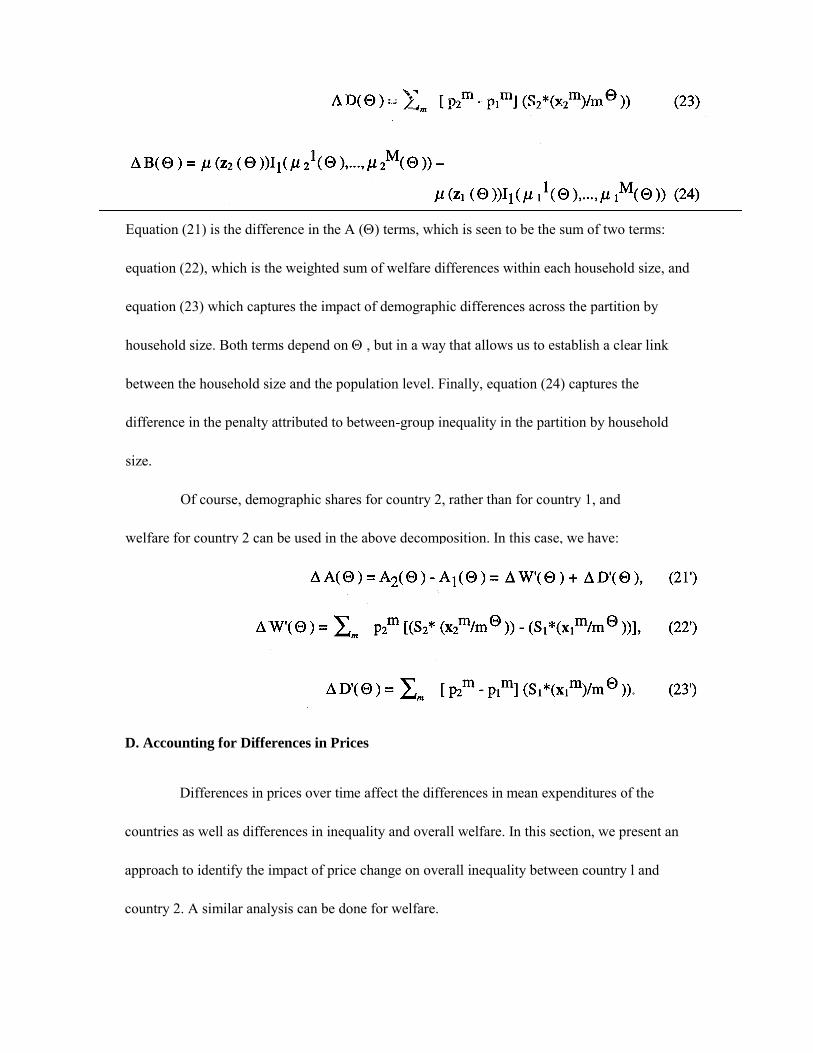
Equation (21) is the difference in the A () terms, which is seen to be the sum of two terms:
equation (22), which is the weighted sum of welfare differences within each household size, and
equation (23) which captures the impact of demographic differences across the partition by
household size. Both terms depend on , but in a way that allows us to establish a clear link
between the household size and the population level. Finally, equation (24) captures the
difference in the penalty attributed to between-group inequality in the partition by household
size.
Of course, demographic shares for country 2, rather than for country 1, and
welfare for country 2 can be used in the above decomposition. In this case, we have:
D. Accounting for Differences in Prices
Differences in prices over time affect the differences in mean expenditures of the
countries as well as differences in inequality and overall welfare. In this section, we present an
approach to identify the impact of price change on overall inequality between country l and
country 2. A similar analysis can be done for welfare.
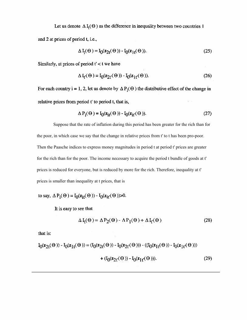
Suppose that the rate of inflation during this period has been greater for the rich than for
the poor, in which case we say that the change in relative prices from t' to t has been pro-poor.
Then the Paasche indices to express money magnitudes in period t at period t' prices are greater
for the rich than for the poor. The income necessary to acquire the period t bundle of goods at t'
prices is reduced for everyone, but is reduced by more for the rich. Therefore, inequality at t'
prices is smaller than inequality at t prices, that is
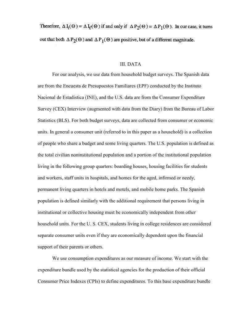
III. DATA
For our analysis, we use data from household budget surveys. The Spanish data
are from the Encuesta de Presupuestos Familiares (EPF) conducted by the Instituto
Nacional de Estadistica (INE), and the U.S. data are from the Consumer Expenditure
Survey (CEX) Interview (augmented with data from the Diary) from the Bureau of Labor
Statistics (BLS). For both budget surveys, data are collected from consumer or economic
units. In general a consumer unit (referred to in this paper as a household) is a collection
of people who share a budget and some living quarters. The U.S. population is defined as
the total civilian noninstitutional population and a portion of the institutional population
living in the following group quarters: boarding houses, housing facilities for students
and workers, staff units in hospitals, and homes for the aged, infirmed or needy,
permanent living quarters in hotels and motels, and mobile home parks. The Spanish
population is defined similarly with the additional requirement that persons living in
institutional or collective housing must be economically independent from other
household units. For the U. S. CEX, students living in college residences are considered
separate consumer units even if they are economically dependent upon the financial
support of their parents or others.
We use consumption expenditures as our measure of income. We start with the
expenditure bundle used by the statistical agencies for the production of their official
Consumer Price Indexes (CPIs) to define expenditures. To this base expenditure bundle
14

the winter of 1981. Since we use household specific price indices, we are able to take
into account the distributional role of changes in price relatives during the 1980's in
both countries.
For comparing expenditures and welfare in the two countries, we use purchasing
power parities (PPPs) for private consumption expenditures. These are rates of currency
conversion that equalize the purchasing power of the two countries. This means that a
given sum of money, when converted into different currencies at the PPP rates, will buy
the same basket of goods and services. PPPs have the advantage over exchange rates in
that they reflect only differences in the volume of goods and services purchased; in
contrast, exchange rates reflect both differences in the volumes purchased in each
country and also differences in price levels. PPPs based on the Elteto-Koves-Szulc (EKS)
method of aggregation are used (DECD 1993). Although the EKS indexes are not
additive, the DECD notes that the EKS can be used to compare levels? The EKS indexes
are used since we are interested in comparing levels of expenditures and welfare. For
1991, the PPP conversion factor is 108.9 so that Spanish expenditures in pesetas are
divided by 108.9 to obtain Spanish expenditures in U.S. dollars. For 1981, the PPP
conversion factor is 74.74 (Godbout 1997; DECD 1993).
7An alternative is to use the Geary-Khamis (GK) index which is additive. This index is most appropriate to use when comparing structures and applying subindexes such that the sum of the adjusted subcomponent expenditures, for example, will equal total PPP adjusted expenditures. Since we are using the overall index and not subcomponent indexes to make our PPP adjustments for total expenditures, it is acceptable to use the EKS indexes. Dukhanov (1997) has noted that substantial differences result however when the two different indexes are used in adjusting subcomponents and then adding up to produce overall national account incomes, for example. However, for our study, we do not expect major differences, given that the GK PPP index for 1981 is 73.3 (versus 74.74) and the index for 1991 is and 106.8 (versus 108.9).
16

For all analyses, consumer unit population weights are used. For the U.S., the
average consumer unit weight for the number of quarters that the consumer unit is in
the sample is used; for the household size variable, the average size is also assumed.
A. Spanish Data
The Spanish EPF is a household budget survey in which interviews are spread
out uniformly over a period of 52 weeks. All household members, 14 years of age or
older, are supposed to record all expenditures taking place during a sample week. Then
indepth interviews are conducted to register past expenditures over reference periods
beyond a week and up to a year. From that information the INE estimates annual
household total expenditures. Annual expenditures on food and drinks in Spain take into
account the available information on bulk purchases according to the procedure
developed in Pena and Ruiz-Castillo (1995). For our study, annual household total
expenditures, based on this set of different reporting periods, are assigned the reference
1990-91 period according to the quarter in which the interview took place.
Data from the two most recent EPFs, collected from April 1980 to March 1981
and from April 1990 to March 1991, are used for our analysis (for details on the 1980-81
and 1990-91 surveys, respectively, see INE (1983) and INE (1992)). In the 1990-91
period, approximately 23,000 households were included in the sample. These households
represent 11,298,509 households in the population and 38,494,006 persons.
B. U.S. Data
The U.S. CEX has two components: a Diary or recordkeeping survey completed
by participating consumer units for two consecutive one-week periods, and an Interview
survey in which the expenditures of consumer units are obtained in five interviews
17

conducted every three months. Survey participants record dollar amounts for goods and
services purchased during the week of data collection for the Diary and during the
previous three months (from the date of the interview) for the Interview. The
expenditure amounts (full purchase price regardless of financing with the exception of
vehicles and housing) include all sales and excise taxes for all items purchased by the
consumer unit for itself or for others. Excluded from both surveys are all
business-related expenditures and expenditures for which the consumer unit is
reimbursed.
The Interview sample is selected on a rotating panel basis, targeted at 5,000
consumer units each quarter. About twenty percent of the sample are interviewed for
the first time each quarter while twenty percent are interviewed for the last time.
Consumer units are interviewed up to five times, at three-month intervals. Data from
the first interview are used to `bound' expenditures for subsequent interviews and are
not used in estimation.
Since we are interested in total expenditures, we use data from both the Diary
and Interview following a method developed by Rob Cage at the BLS (Cage et al. 1997.
The BLS (1995) estimates that about 80 to 95 percent of all expenditures are accounted
for in the Interview. Not accounted for in the Interview are roughly 40 specific goods
and services, e.g., soaps, laundry and cleaning products, tolls, over-the counter drugs, pet
food, and personal care products. We use data from the Diary to impute additional
expenditures for these omitted items to the Interview households. This was
accomplished by calculating the expenditure for the Diary-unique item, as a percent of
total food expense, and taking the product of this factor and the total food expense
reported in the Interview. The budget shares for these items were produced by
index-area and consumer
18
unit size in the Diary sample. These shares were then mapped to the CEX Interview
sample by index area and consumer unit size, and used to impute expenditures for
these additional items in the Interview.
The continuous and rotating nature of the CEX Interview in the U.S. case poses
special problems for the determination of the 1990-91 household expenditures
distribution at current prices, that is, the equivalent of the expenditure distribution in the
Spanish case. We limit ourselves to the Interview survey consumer units only, since
these consumer units provide the maximum of data over the longest period of time,
relative to the Diary sample. For our analysis we do not assume that the quarterly
expenditure reports are independent (as in official CEX publications, see BLS 1995), but
require each consumer unit to have reported expenditures for two, three, or four quarters
during the time period of our study. We refer to our sample as horizontal. Restricting
ourselves to households with four quarters of complete data would have been
unnecessarily restrictive, while including some incomplete households allows us to
increase the sample size. If we selected our households with interviews occurring over
the exact time period as in the Spanish case (Summer 1990 to Spring 1991), there would
only be 1,367 consumer units in the U.S. sample. In contrast, our horizontal sample is
composed of 6,284 consumer units, representing 118,481,815 consumer units in the
population and 307,204,548 persons. The U. S. data were collected from January 1990 to
December 1991. Data from the reported quarters, during this time period, are used to
produce annualized expenditures for each consumer unit. The consumer unit
characteristics of household size8 and age of head are based on the average of the ______________________________ 8 Rounded values of average household size were used for our analysis.
quarterly values for the values reported. The population weights used for our analysis
are also the result of averaging the quarterly weights over the number of quarters for
which the consumer unit participates in the survey.
IV. RESULTS
Our study confirms that, in international comparisons, demographic structure and
prices are important. In this section we examine the population distributions by
household size, expenditures of households, inequality, and welfare. Unadjusted
expenditures are used for the inequality analysis when we examine within group
differences by household size. However, adjusted expenditures are used when examining
overall inequality since between group differences are dependent on the adjustment
factor. Since welfare for each household size depends on the scale adjustment factor, we
present the unadjusted values by household size, but focus most of our attention on the
results for all persons.
As shown in Table 1, we observe one and two person households in the U.S. are
more numerous and have much greater mean expenditures than those in Spain. For three
person households, representing about 20 percent of all persons in each country, mean
expenditures are still substantially higher for the U.S. For four person households,
representing about 30 percent of all persons in Spain and 24 percent in the U.S., mean
expenditures are greater in the U.S., but not as great as for smaller household sizes.
Except for six person households, larger households have greater mean levels of
expenditures in the U.S.

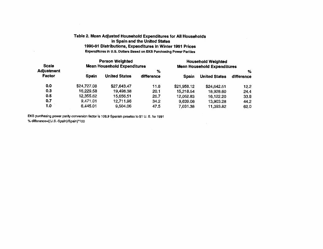
The results in Table 2 illustrate the impact on means expenditures of using person
versus household weighting. With person weighting, each person in a household is
assigned the adjusted expenditure while with household weighting each household only
is assigned a weight of 1. This means persons living in larger households will have more
weight in the overall distribution of expenditures. When comparing the person weighted
and household weighted expenditures, expenditures are greater in the U.S. relative to
those in Spain for each scale adjustment factor. However, when comparing person
weighted versus household weighted expenditures for each country, household weighted
expenditures are less than person weighted expenditures when the scale factor
adjustment is smaller for the U.S. (= 0.0 or 0.3). The pattern is more pronounced for
Spain; household weighted expenditures are less for all scale adjustment factors other
than for the per capita adjustment ( =1.0).
The Theil indexes for households of size one to seven, based on expenditures in
winter 199-91 prices, are presented in Table 3. As noted earlier, the parameter c (here
equal to -1, 0, 1, and 2) summaries the sensitivity of the inequality index in different parts
of the expenditure distribution: the more positive (negative) c is, the more sensitive the
index is to differences at the top (bottom) of the distribution. For both the U.S. and Spain,
inequality is greater when c=-1 than when c=0, and also when c=2 versus c=1. In general,
inequality in Spain is greatest when c=2 across household sizes. For the U.S., inequality
is greatest when c=-1 or c=2, with greater values for c=-1 for households with three, four,
five, or seven members. Inequality in the U.S. is less than inequality in Spain for one and
two person households when c=-1, 0, or 1. Thus we could conclude that differences at the
lower end of the distribution are greater for Spain than for the U.S. for
21
these households. When c=2, inequality is less in the U.S. for households with
fewer than five persons. For these households we can surmise that the differences in
expenditures at the top of the Spanish distribution are greater than the differences in
expenditures at the top of the U.S. distribution.
The use of decomposable inequality measures facilitates our understanding of the
results for the population as a whole. In particular, for the person weighted distributions
(Table 4), within group inequality is smaller in Spain than in the U.S., while the results
on overall inequality depend crucially on our assumptions about the importance of
economies of scale (denoted by our scale adjustment factors). As the scale adjustment
factor ( ) varies from 0 to 1 and economies of scale tend to diminish, overall inequality
in the U.S. is smaller, about the same, or considerably larger than in Spain. This
difference is due to the between group differences in inequality.
Concerning the influence of prices, our results reveal that changes in relative
prices from the winter of 1981 to the winter of 1991 are pro-poor in both countries
(Table 5). This means that from the point of view of winter 1981, the amount that we
would need to give to richer households to compensate them for inflation would be
greater than the amount that we would need to give to poorer households for them to
remain at the same level of welfare. However, in Spain the strength of this phenomenon
decreases with household size, while the opposite is the case in the U.S. The percentage
difference in inequality in the U.S. 1990-91 expenditure distribution relative to the
Spanish one is rather robust to the choice of the reference price vector. The percentage
differences in inequality in the U.S. relative to Spain are sensitive to household size and
to our choice of
22
the scale adjustment factor. For households of size 1 or 2 and when the scale
adjustment factor equals 0.0 or 0.3, inequality is greater in Spain.
Recall that welfare is equal to mean expenditures corrected by a factor related to
inequality. For the welfare analysis, we use the Theil inequality index with c=1. In Table
6 we present overall welfare for households with one to seven members. For this table,
unadjusted expenditures are used. The differences in welfare exhibit the same pattern as
for the means presented in Table 2. Welfare is greater in the U.S. than in Spain for all
households with the exception of those with six members.
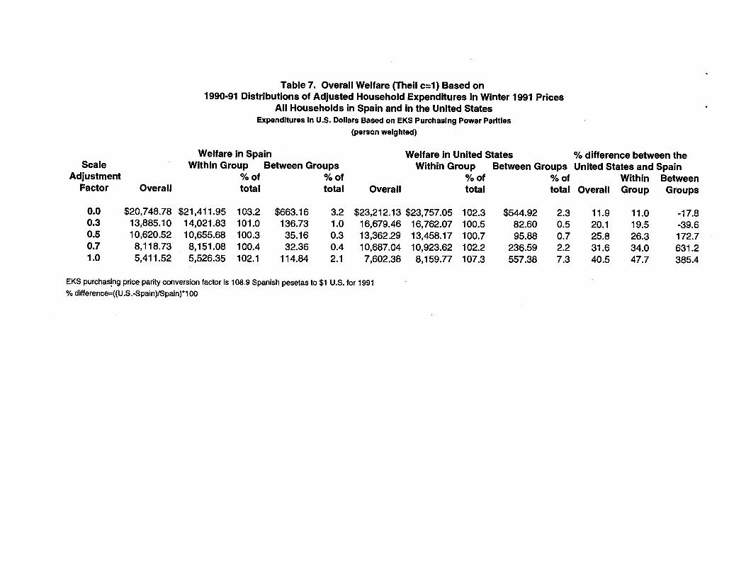
Not surprisingly, results presented in Table 7 indicate greater overall welfare for
households in the U.S. as compared to those in Spain regardless of the value of . The
greatest percentage of this difference is due to differences in within group inequality.
Between group inequality is greater in Spain than in the U.S. when = 0.0 or 0.3. Thus,
for the U.S.-Spanish case, we conclude that between group inequality is sensitive to the
assumption about economies of scale.
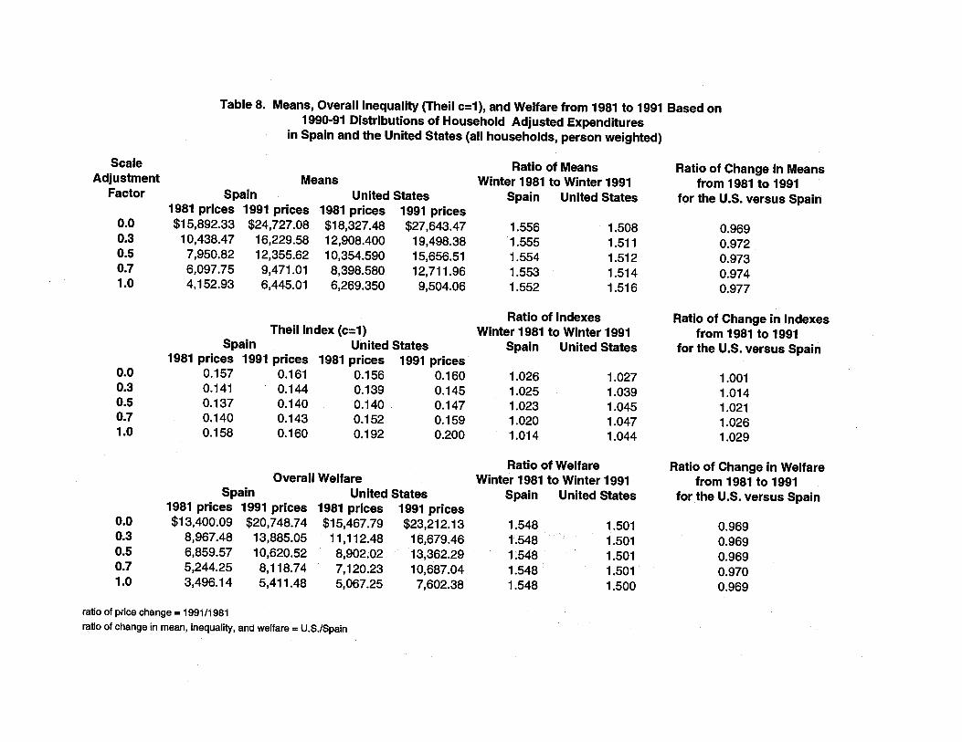
The influence of changing prices on welfare can be examined using the results
presented in Table 8. The change in welfare is a function of the ratio of the change in
mean expenditures and the change in inequality when inequality is defined as the Theil
index with the parameter c=1. When changes in prices are greater in the U. S. relative to
Spain, the ratio of the differences in means will be less than one. Since inequality, as
measured by the Theil index with c=1, is dependent upon the scale adjustment factor,
the ratio of the differences in inequality in the U.S may be less than, equal to, or greater
than inequality in Spain. If the index value is greater in period two than in period one,
then prices can be considered to be pro-poor. Thus we cannot predict the whether the
23
differences in welfare are greater in the U.S. than in Spain when prices from one
period are used versus those from another period. The ratio of the means is the impact
of inflation on mean expenditures, the inequality indexes, and welfare.
As seem in Table 8, for all adjusted expenditures, inflation is greater over the
1981 to 1991 period in Spain than in the U.S. The impact on welfare is slightly less.
Inequality in 1981 and 1991 for both countries is similar. However, in contrast to the
impact on means, the impact of inflation on inequality is marginally greater in the
U.S. than in Spain. The result of these divergent influences of inflation are reflected
in the ratios of welfare at the two price vectors.
The ratios of the changes in the means, indexes, and welfare from 1981 to 1991
are presented in the last two columns of the Table 8. When the ratio is less than one, the
impact of price change in the U.S. is less than the impact of price change in Spain. Our
results reveal that the effect of price change in the U.S. is greater in the U.S. than for
Spain for the means and for overall welfare. However, the influence on inequality is in
the opposite direction.
V. SUMMARY AND CONCLUSIONS
The purpose of this research was to examine the role of demographics and
household specific price indices on expenditure based inequality and welfare
comparisons for Spain and the U.S. Equivalence scales were assumed to depend only on
household size. The 1990-91 expenditure distributions in both countries were expressed
at winter of 1991 and winter of 1981 prices. Our results show that differences in
demographic factors can be very important in international comparisons. We find that
inequality and welfare
24

comparisons are drastically different for smaller and larger households. Given this
diversity, decomposable measurement instruments help to explain how results at the
household size level get translated at the population level. In terms of the influence of
relative prices on inequality, for both countries, prices are pro-poor. This implies that we
would need to give more income to richer households than to poorer households to
compensate them for inflation, over the 1981 to 1991 period. Because the distributional
impact of relative prices is of a comparable order of magnitude, our inequality
comparisons are robust to the choice of the reference price vector. When examining the
impact of changes in overall welfare over time and across the two countries, we found
less change in the U.S. in means and overall welfare, but greater changes in inequality.
In future analyses we plan examine the impact on inequality and welfare of
demographic changes across partition subgroups (due to shifts in subgroup population
shares over time), in addition to the impact due to differences in tastes and preferences as
reflected in expenditures from an earlier period of time. Decompositions by other
demographic subgroups would also be useful in helping us understand the differences
that we obtain for Spain and the U.S.
25
VI. REFERENCES
Atkinson, A. B., L. Rainwater and T. Smeeding (1995), Income Distribution in
DECD Countries: the Evidence from the Luxembourg Income Study (LIS). Paris: OECD.
Bureau of Labor Statistics (1995). Consumer Expenditure Survey, 1992-93, U.S.
Department of Labor, Bureau of Labor Statistics, Bulletin 2462. Washington, D. C.: U.S. Government Printing Office, September.
Buhmann, B., L. Rainwater, G. Schmauss and T. Smeeding (1988), "Equivalence Scales, Well-Being, Inequality and Poverty: Sensitivity Estimates Across Ten Countries Using the Luxembourg Income Study Database," The Review of Income and Wealth, 34: 115-142.
Burkhauser, R., T. Smeeding and J. Merz (1996), "Relative Inequality and Poverty in Germany and the United States Using Alternative Equivalence Scales," The Review of
Income and Wealth, 42: 381-400. Cage, Robert, Thesia I. Garner, and Javier Ruiz-Castillo (1997), "Constructing Household Specific Consumer Price Indexes: An Analysis of Different Techniques and Methods," unpublished manuscript, Division of Price and Index Number Research, Bureau of Labor Statistics, U.S. Department of Labor, Washington, D. C.; prepared for the 1997 National Bureau of Economic Research Summer Institute, Price Index Measurement Workshop, Cambridge, Massachusetts, July 22, 1997. Coulter, F., F. Cowell and S. Jenkins (1992a), "Differences in Needs and Assessment of Income Distributions," Bulletin of Economic Research, 44: 77124. Coulter, F., F. Cowell and S. Jenkins (1992b), "Equivalence Scale Relativities and the Extent of Inequality and Poverty," Economic Journal, 102: 1067-1082. Cowell, F. A. and K. Kuga (1985), "Inequality Measurement: An Axiomatic Approach," European Economic Review, 15: 287-305. Del Rio, C. and J. Ruiz-Castillo (1997a), "Intermediate Inequality and Welfare. The Case of Spain, 1980-81 to 1990-91 ", Universidad Carlos III de Madrid, Working Paper 96-03, Economic Series 03. Del Rio, C. and J. Ruiz-Castillo (1997b), "An Inequality Decomposition Method Which Minimizes Equivalence Scales 'Contamnination' Problems", Universidad Carlos III de Madrid, Working Paper 97-37, Economic Series 15. Dikhanov, Yuri (1997), "Neutralizing Substitution Bias while Retaining Additivity in U.S. National Accounts," unpublished manuscript, Statistical Advisory Services, Development Economics, World Bank, September 1997.
Dutta, B. and J. M. Esteban (1992), "Social Welfare and Equality," Social Choice
and Welfare, 50: 49-68. Godbout, Todd M. (1997). Personal communication concerning calculation of PPPs using data from the OECD with data file maintained by the U.S. Bureau of Labor Statistics, Office of Productivity and Technology, Division of Foreign Labor Statistics and Trade, Washington, D. C., March 12.
Johnson, David and Stephanie Shipp (1997), "Trends in Inequality in ConsumptionExpenditures: The U.S. from 1960 to 1993," Review of Income and
Wealth, June. Organization for Economic Co-Operation and Development (OECD 1993), Statistics Directorate, Purchasing Power Parities and Real Expenditures, EKS Results, Volume 1, Parities de Pouvoir d'Achat et Depenses Reelles, OCED: Paris.
Pena, D. and J. Ruiz-Castillo (1995), "Inflation and Inequality Bias in the Presence of Bulk Purchases for Food and Drinks," Universidad Carlos III de Madrid, Working Paper 95-47, Statistics and Econometrics Series 15.
Phipps, S. and T. Garner (1994), "Are Equivalence Scales the Same for the United States and Canada?,"The Review of Income and Wealth, 40: 1-18.
Rodrigues, C. F. (1993), "Measurement and Decomposition of Inequality in Portugal, 1980/81-1990/91," Department of Applied Economics, University of Cambridge, E.S.R.C. Discussion Paper, MU 9302. Ruiz-Castillo, J. (1995a), "Income Distribution and Social Welfare: A Review Essay," Investigaciones Economicas, XIX: 3-34. Ruiz-Castillo, J. (1995b), "The Anatomy of Money and Real Inequality in Spain, 1973-74 to 1980-81," Journal of Income Distribution, 5: 265-281. Ruiz-Castillo (forthcoming 1998), "A Simplified Model for Social Welfare Analysis. An Application to Spain, 1973-74 to 1980-81," Review of Income and Wealth.
Ruiz-Castillo, J. and M. Sastre (1997), "La construccion de indices de precios con base en 1983 para los hogares de las EPF de 1980-81 y 1990-91," unpublished manuscript, Universidad Carlos III de Madrid. Shorrocks, A. F. (1984), "Inequality Decomposition by Population Subgroups," Econometrica, 52: 1369-1388.