The Inflation Response to Government Spending Shocks:

A Fiscal Price Puzzle?∗

Peter L. Jørgensen† Søren H. Ravn‡

July 2018

Abstract

This paper provides empirical evidence that prices decline significantly and persis-

tently in response to a positive government spending shock. This result stands out

across a wide variety of specifications of our Structural Vector Autoregression (SVAR)

model and for different price indices. The decline in prices is accompanied by an increase

in output and private consumption, as found in most of the existing literature, as well

as an increase in Total Factor Productivity. These findings are hard to reconcile with

standard New Keynesian models with exogenous productivity, which typically generate

higher prices and a drop in consumption following a fiscal expansion. We show that the

introduction of variable technology utilization can enable an otherwise standard New

Keynesian model to match our empirical findings. Variable technology utilization al-

lows firms to accommodate an increase in demand by adopting new technology into the

production process. The resulting increase in measured productivity leads to a decline

in prices and an increase in consumption.

Keywords: Government Spending Shocks, Fiscal Policy, Business-cycle Comove-

ment, DSGE Modelling, Endogenous Productivity.

JEL classification: E13, E31, E32, E62.

∗The authors wish to thank Philippe Aghion, Wouter Den Haan, Giulio Fella, Ethan Ilzetzki, HenrikJensen, Albert Marcet, Emi Nakamura, Gisle Natvik, Ivan Petrella, Giorgio Primiceri, Ricardo Reis, Emil-iano Santoro, and Jon Steinsson for useful comments and discussions. Part of this work was carried out whileRavn was visiting the Centre for Macroeconomics at the London School of Economics, and while Jørgensenwas a PhD student at the University of Copenhagen and Danmarks Nationalbank. The hospitality of theseinstitutions is kindly acknowledged. The usual disclaimer applies.†Address: Department of Economics, Lund University, Tycho Brahes Väg 1, 220 07 Lund, Sweden Email:

peter.jorgensen@nek.lu.se.‡Corresponding author. Address: Department of Economics, University of Copenhagen, Øster Farimags-

gade 5, building 26, DK-1353 Copenhagen, Denmark. Email: soren.hove.ravn@econ.ku.dk. Phone: +45 2655 73 35.

1 Introduction

The macroeconomic effects of changes in government spending have received widespread

attention in the economics profession, not least since the onset of The Great Recession

in 2007. Following the tradition of Blanchard and Perotti (2002), a large literature has

employed Structural Vector Autoregressive (SVAR) models to characterize the empirical

effects of government spending shocks on GDP, private consumption, and a range of other

macroeconomic variables (e.g., Ramey, 2011a). However, the response of inflation to gov-

ernment spending shocks has typically received limited attention in the empirical literature.

Nonetheless, the conventional wisdom is that increases in government spending are infla-

tionary. Indeed, this idea plays an important role in the transmission of fiscal policy shocks

in several theoretical models, including the textbook New Keynesian model. A prominent

example is the effectiveness of government spending shocks when the nominal interest rate

is at the zero lower bound. The finding of a large fiscal multiplier under these circumstances

relies entirely on the ability of higher government spending to drive up (expected) inflation

and thus reduce the real interest rate (e.g., Christiano et al., 2011).1 In this paper, we

study the effects of government spending shocks on prices in the U.S. economy using an

SVAR approach. Our main finding is that prices decline significantly and persistently in

response to an increase in government spending. This result stands out across a variety of

specifications of our empirical model, as well as across different price indices and identifi-

cation strategies. Importantly, the drop in prices coexists with the increase in output and

private consumption found in most of the existing literature (e.g., Blanchard and Perotti,

2002; and Galí et al., 2007). Moreover, we observe an increase in Total Factor Productivity

(TFP). We show that an otherwise standard New Keynesian model augmented with variable

technology utilization can account for these empirical findings.

The existing evidence on the response of prices to government spending shocks is rather

mixed, as illustrated in Table 1. Some previous studies, including Fatas and Mihov (2001b)

and Mountford and Uhlig (2009), have also reported a decline in prices in response to a

fiscal expansion in the US. However, other authors– for example, Edelberg et al. (1999) and

Caldara and Kamps (2007)– report that prices increase, while yet others– e.g., Nakamura

and Steinsson (2014)– find an insignificant response. Perotti (2004) finds mixed evidence of

the response of inflation in the US and four other OECD countries, but concludes that there

is little evidence in support of the common perception that government spending shocks

are inflationary.2 Several prominent studies of fiscal policy do not consider the response of

1Another example emerges from open-economy models: The fiscal multiplier is typically found to besmaller in countries with floating exchange rates (as compared to countries with a currency peg), as theywill experience a tightening of monetary policy to combat the rise in inflation assumed to follow an increasein government spending (e.g., Corsetti et al., 2013).

2As seen in Table 1, some studies report the response of the price level, and others that of the inflation

1

prices at all, and most of the authors who do find evidence of a decline in inflation do not

attempt to provide a structural explanation for it.3

Table 1: Empirical Estimates of Inflation Response

Fiscal Policy Study Response of Prices/Inflation

Edelberg et al. (1999) Prices increase

Fatas and Mihov (2001a) Prices are insignificant

Fatas and Mihov (2001b) Prices decline

Blanchard and Perotti (2002) Not reported

Canzoneri et al. (2002) Inflation declines

Burnside et al. (2004) Not reported

Perotti (2004) Mixed response of inflation

Canova and Pappa (2007) Mixed response of prices

Galí et al. (2007) Not reported

Caldara and Kamps (2008) Inflation increases

Mountford and Uhlig (2009) Prices decline

Ramey (2011a) Not reported

Nakamura and Steinsson (2014) Inflation is insignificant

Dupor and Li (2015) Prices decline or are insignificant

Ben Zeev and Pappa (2017) Inflation increases

D’Alessandro and Fella (2017) Inflation declines

Ricco et al. (2017) Inflation declines or is insignificantNotes: In Edelberg et al. (1999), the GDP deflator increases, while the CPI index first increases

and then declines. In Fatas and Mihov (2001b) and Canzoneri et al. (2002), the decline in inflation

is barely significant. All studies use U.S. data, though Perotti (2004) and Canova and Pappa (2007)

also report evidence from other OECD countries and from Euro Area countries, respectively.

Our empirical findings are hard to reconcile with traditional accounts of the transmission

mechanism of fiscal policy. To provide a structural interpretation of our results, we therefore

propose a version of the New Keynesian model featuring time-varying adoption of new

technology into the production process, as in recent work by Anzoategui et al. (2017)

and Bianchi et al. (2017). In our model, firms decide on the extent to which they utilize

the available technology level. In response to an increase in government spending, firms

rate, but this cannot explain the different findings in the literature. While we use the price level in all ourestimations, none of our findings depend on this choice.

3Canova and Pappa (2007) offer a discussion of potential explanations for a decline in prices after a fiscalexpansion, of which they find some evidence, but they stop short of proposing a theoretical model.

2

find it optimal to raise the utilization rate of technology in order to meet the increase in

aggregate demand, despite the costs associated with a higher utilization rate. An increase in

technology utilization raises measured productivity, in line with the empirical evidence we

present. Provided this mechanism is suffi ciently powerful, it dominates the upward pressure

on marginal costs stemming from higher wages, thus ensuring that marginal costs decline

in equilibrium. This paves the way for firms to reduce their prices, generating the desired

decline in inflation. In turn, this induces the central bank to reduce the nominal interest

rate, in line with what we observe in our SVAR evidence. This leads to a drop in the real

interest rate, facilitating an increase in consumption.

The theoretical model is deliberately simple in order to allow for an analytical solution.

As in the basic New Keynesian model, combining a standard consumption Euler equation

with a version of the Taylor rule for monetary policy results in a negative relationship

between consumption and inflation. In our model, an increase in government spending

shifts the economy down along this consolidated Euler equation, resulting in a decline in

inflation and an increase in consumption, in line with the data. We provide an analytical

characterization of the parameter requirements for our model to generate these findings,

and show that a range of parameters always exists for which this is the case. We also show

that a calibrated version of our model can account for the dynamic effects of government

spending shocks in the data for reasonable parameter values. Finally, we introduce capital

formation into the model and estimate the key parameters using indirect inference, thus

confirming our findings in a more realistic model environment.

Incidentally, the textbook version of the New Keynesian model typically features a neg-

ative comovement between inflation and private consumption conditional on a shock to

government spending, but of the opposite sign than what we find in the data: inflation

increases and consumption declines after a positive government spending shock. The re-

sponse of consumption has received widespread attention in the theoretical literature, with

several authors proposing mechanisms to obtain an increase in consumption. However, most

of these seem to hold little promise for producing a decline in inflation. For example, the

introduction of rule-of-thumb households by Galí et al. (2007) drives up aggregate demand

but has no direct effects on the supply side. Allowing for non-separable utility in consump-

tion and leisure, as in Monacelli and Perotti (2008) and Bilbiie (2011), induces consumption

and labor supply to increase in tandem, provided consumption and leisure are substitutes.

However, as shown by Bilbiie (2011), the demand-side effects still dominate, leading to a

rise in inflation.

Correspondingly, while theoretical models exist that may potentially be able to generate

a decline in inflation after a fiscal expansion, these are generally not consistent with a con-

temporaneous increase in consumption. In the New Keynesian model, there are essentially

3

three ways to bring about a drop in inflation in response to a government spending shock:

a drop in the markup, a drop in the wage rate, or an increase in productivity. A counter-

cyclical markup is the hallmark of the so-called deep habits model of Ravn et al. (2006),

who show that this mechanism can even generate an increase in consumption after a gov-

ernment spending shock in their flexible-price model. However, Jacob (2015) demonstrates

that the deep habits model performs quite differently in sticky-price environments: while it

may indeed generate a decline in inflation, this occurs alongside a decline in consumption.4

A drop in the wage rate may be obtained in the presence of a suffi ciently strong increase in

labor supply in response to the reduction in permanent income associated with higher gov-

ernment spending (Baxter and King, 1993). Besides requiring an implausibly large Frisch

elasticity of labor supply, however, a declining wage makes it very unlikely to observe an

increase in consumption, as shown, e.g., by Monacelli and Perotti (2008).5 Altogether, these

considerations lead us to focus on endogenous changes in the level of productivity as a more

promising avenue for matching the empirical evidence.

We contribute to an emerging literature studying endogenous changes in productivity

over the business cycle. We build directly on the work of Bianchi et al. (2017), who pro-

pose an endogenous growth model capturing both business-cycle fluctuations and long-term

growth. In their model, endogenous variations in TFP can arise due to variable technology

utilization or R&D investments in “knowledge capital”. At business-cycle frequencies, they

find that variations in technology utilization account for the bulk of fluctuations in TFP,

whereas the accumulation of knowledge capital is important for long-term growth. While

the model of Bianchi et al. (2017) features endogenous technological progress through ver-

tical innovations, as in Aghion and Howitt (1992), other authors have employed horizontal

innovations featuring increasing returns to specialization as in Romer (1990) and Comin

and Gertler (2006). A prominent recent example is the paper by Anzoategui et al. (2017),

who find that most of the observed decline in TFP during the Great Recession can be

attributed to endogenous factors, primarily a decline in the intensity of technology adop-

tion. Moran and Queralto (2018) use a similar model to study the link between monetary

policy shocks and endogenous movements in technology after establishing that a monetary

expansion leads to an increase in TFP in the data. More generally, several recent papers

have pointed to various types of demand shocks as potentially important drivers of fluctu-

ations in TFP over the business cycle. Notable examples are Bai et al. (2017) and Benigno

and Fornaro (2017). However, none of these papers study the connection between endoge-

4 In a nutshell, price stickiness erodes the ability of firms to reduce their markup as desired under deephabits, thus impeding the increase in real wages necessary to drive up consumption.

5An alternative way to obtain a decline in the wage rate is to allow for a suffi ciently strong reaction ofmonetary policy to output, as shown by Linnemann and Schabert (2003). Aside from the fact that an increasein the nominal interest rate is in contrast to our empirical evidence, this approach has the disadvantage ofleading to an even larger drop in consumption.

4

nous productivity and fiscal policy. In this respect, two existing studies are more closely

related to our paper. Aghion et al. (2014) find that systematic, countercyclical fiscal pol-

icy can have positive long-term effects on productivity growth. To rationalize this finding,

they devise a model in which countercyclical fiscal policy leads to a reduction in business-

cycle volatility, which in turn facilitates investments in productivity-enhancing long-term

projects, such as R&D investments. D’Alessandro and Fella (2017) propose a business-cycle

model with learning-by-doing, and show that it can generate positive responses of private

consumption, the real wage, and TFP to a government spending shock, in line with their

empirical evidence. While this mechanism may potentially complement the one we propose,

their full-fledged model with capital generates an increase in inflation on impact, in contrast

with the empirical results we present.6

Finally, our findings are reminiscent of the so-called “price puzzle”of monetary policy

(Sims, 1992). Upon confirming that our results do not suffer from common types of mis-

specification that have been proposed in this regard (notably, the drop in prices is confirmed

when commodity prices are included in the VAR model), we propose a structural expla-

nation sharing some features with the cost channel of monetary policy proposed by Barth

and Ramey (2002) to account for the monetary price puzzle. Both mechanisms rely on

supply-side effects to produce a reduction in marginal costs in response to an expansionary

demand shock. Our results are also related to the puzzling behavior of the real exchange

rate in connection with fiscal policy in open economies. Kim and Roubini (2008), Monacelli

and Perotti (2010), and Ravn et al. (2012) all find that the real exchange rate depreciates in

response to an expansionary government spending shock, i.e. that domestic prices decline

relative to foreign (exchange-rate-adjusted) prices.

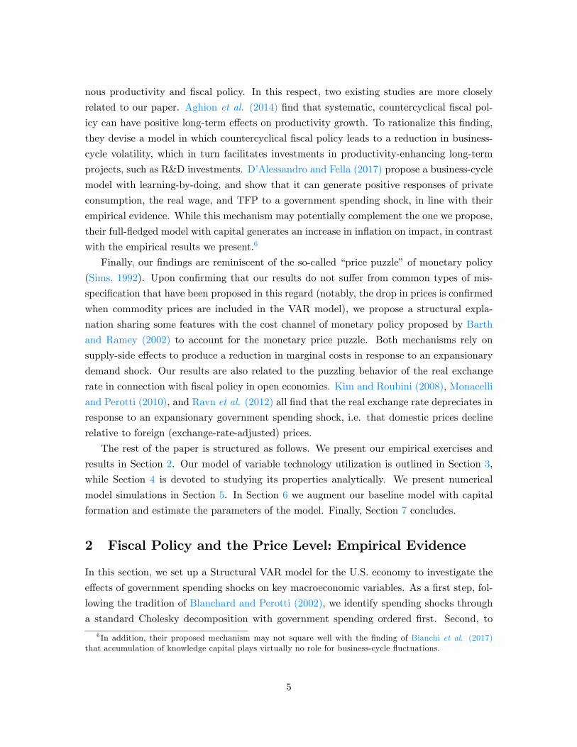
The rest of the paper is structured as follows. We present our empirical exercises and

results in Section 2. Our model of variable technology utilization is outlined in Section 3,

while Section 4 is devoted to studying its properties analytically. We present numerical

model simulations in Section 5. In Section 6 we augment our baseline model with capital

formation and estimate the parameters of the model. Finally, Section 7 concludes.

2 Fiscal Policy and the Price Level: Empirical Evidence

In this section, we set up a Structural VAR model for the U.S. economy to investigate the

effects of government spending shocks on key macroeconomic variables. As a first step, fol-

lowing the tradition of Blanchard and Perotti (2002), we identify spending shocks through

a standard Cholesky decomposition with government spending ordered first. Second, to

6 In addition, their proposed mechanism may not square well with the finding of Bianchi et al. (2017)that accumulation of knowledge capital plays virtually no role for business-cycle fluctuations.

5

account for anticipated changes in fiscal policy, we use the forecast errors of government

spending computed by Auerbach and Gorodnichenko (2012) to identify shocks to govern-

ment spending. To check the robustness of our results, we consider a vast number of

alternative specifications of our VAR model, as well as alternative identification schemes.

We estimate the following quarterly VAR model on U.S. data:

Xt = a0 + a1t+ a2t2 +B−1A(L)Xt−1 +B−1et, (1)

where Xt is the vector of endogenous variables, et is a vector of i.i.d. structural shocks

with unit variance, A(L) comprises the coeffi cients on the lagged endogenous variables, L

is the lag operator and B comprises the coeffi cients on the contemporaneous endogenous

variables. We include linear and quadratic time trends, as in Blanchard and Perotti (2002).

We follow most of the literature and use 4 lags as our baseline. Our data sample covers

the period 1960:Q1-2017:Q2. We use the following variables in our analysis: Real govern-

ment expenditure and investment (Gt), real GDP (Yt), real private consumption (Ct), real

tax revenue (tax receipts less current transfers, interest payments and subsidies) (Tt), the

Personal Consumption Expenditures (PCE) price index (Pt), the nominal interest rate on

3-month treasury bills (Rt), and Total Factor Productivity (At).7 All variables except Rtare in logs, and the variables Gt, Yt, Ct and Tt are measured in real per-capita terms. Ttis converted into real terms using the GDP deflator. We use the TFP measure of Fernald

(2014).8 Appendix A contains a detailed description of the data.

2.1 The Cholesky Decomposition

Under the Cholesky identification scheme, the model contains the following variables:

Xt =[Gt Yt Ct Tt Pt Rt At

]′.

Following the approach of Blanchard and Perotti (2002), we assume that the structural

shocks to government spending can be recovered from the estimated residuals B−1et in (1)

by imposing that the matrix B is lower triangular. This implies that government spending

does not respond to any other variable within-quarter, but affects other variables within

the same quarter. Intuitively, the assumption is motivated by decision lags in fiscal policy.

By the time policymakers realize that a shock has hit the economy and implement an

appropriate policy response, at least one quarter would have passed.9 The ordering of the7All results are robust if we use non-durable consumption instead of total consumption.8We use the non-utilization-adjusted TFP measure as our baseline. All results are robust to using the

utilization-based measure instead.9This implies that the within-period elasticity of real government spending to a change in prices is

assumed to be zero. In the absence of perfect indexation of government spending, this assumption may not

6

remaining variables is such that real variables (with the exception of TFP) are determined

before nominal ones, and that monetary policymakers are assumed to be able to observe

and react to changes in output and prices within-period. Our findings are robust to different

orderings of the variables.

Figure 1 shows the impulse-response functions to a positive government spending shock

normalized to 1 percent, along with 68 percent bootstrapped confidence bands, obtained

using the delta method with 2, 000 replications. All responses are denoted in percent,

except for the interest rate, where the response is reported in basis points. Following a fiscal

expansion, output and consumption increase persistently, in line with most of the empirical

literature.10 Prices display a strongly significant and very persistent decline. The price

level drops by around 0.3 percent at the peak. The implied annualized inflation rate drops

by slightly more than 25 basis points at its trough 2 quarters after the shock. TFP also

increases significantly, in line with the evidence reported by Bachmann and Sims (2012)

for the US, and by Afonso and Sousa (2012) for four OECD countries including the US.

Finally, the short-term nominal interest rate drops by around 20 basis points, and tax

revenues decline.

2.2 Controlling for Fiscal Foresight: Baseline VAR model

A common criticism of the Cholesky identification strategy employed above is that changes

in fiscal policy are– at least to some extent– anticipated by economic agents, as discussed

by Ramey (2011a), among others. In this case, it is not possible to recover a structural

shock to fiscal policy using the identification strategy of Blanchard and Perotti (2002).

To account for this, we consider an identification scheme that controls for fiscal foresight.

Following Auerbach and Gorodnichenko (2012), we identify an unanticipated government

spending shock as an innovation to the forecast error of the growth rate of government

spending. The vector of endogenous variables becomes:

Xt =[FEt Gt Yt Ct Tt Pt Rt At

]′,

where FEt is the implied forecast error of the survey-based forecasts of the growth rate of

government spending, which we obtain from Auerbach and Gorodnichenko (2012). In order

to recover an unanticipated government spending shock, we order FEt first in the system.

be satisfied. Perotti (2004) suggests that the within-period elasticity of government spending to a change inprices might be as high as −0.5. We have verified that our findings are robust to this choice.10The implied government spending multiplier on output can be found by multiplying the reported output

response by the inverse of the sample average of the ratio of government spending to output, which is 0.245.This implies an impact multiplier of 1.02, well within the range of available estimates reported in the surveyof Ramey (2011b) of 0.8− 1.5.

7

Government Spending

0 10 20 30 40­0.5

0

0.5

1

1.5Output

0 10 20 30 40­0.2

0

0.2

0.4

Private Cons.

0 10 20 30 40­0.2

0

0.2

0.4Taxes

0 10 20 30 40­3

­2

­1

0

1

PCE index

0 10 20 30 40­0.6

­0.4

­0.2

0

0.2Int. Rate

0 10 20 30 40­30

­20

­10

0

10

TFP

0 10 20 30 400

0.1

0.2

0.3

Figure 1: The dynamic effects of a shock to government spending. VAR model with Choleskyidentification scheme. The black line denotes the estimated response, while the grey areasrepresent 68 percent confidence bands.

8

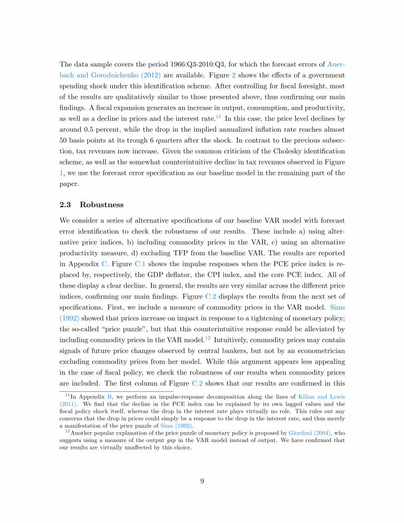
The data sample covers the period 1966:Q3-2010:Q3, for which the forecast errors of Auer-

bach and Gorodnichenko (2012) are available. Figure 2 shows the effects of a government

spending shock under this identification scheme. After controlling for fiscal foresight, most

of the results are qualitatively similar to those presented above, thus confirming our main

findings. A fiscal expansion generates an increase in output, consumption, and productivity,

as well as a decline in prices and the interest rate.11 In this case, the price level declines by

around 0.5 percent, while the drop in the implied annualized inflation rate reaches almost

50 basis points at its trough 6 quarters after the shock. In contrast to the previous subsec-

tion, tax revenues now increase. Given the common criticism of the Cholesky identification

scheme, as well as the somewhat counterintuitive decline in tax revenues observed in Figure

1, we use the forecast error specification as our baseline model in the remaining part of the

paper.

2.3 Robustness

We consider a series of alternative specifications of our baseline VAR model with forecast

error identification to check the robustness of our results. These include a) using alter-

native price indices, b) including commodity prices in the VAR, c) using an alternative

productivity measure, d) excluding TFP from the baseline VAR. The results are reported

in Appendix C. Figure C.1 shows the impulse responses when the PCE price index is re-

placed by, respectively, the GDP deflator, the CPI index, and the core PCE index. All of

these display a clear decline. In general, the results are very similar across the different price

indices, confirming our main findings. Figure C.2 displays the results from the next set of

specifications. First, we include a measure of commodity prices in the VAR model. Sims

(1992) showed that prices increase on impact in response to a tightening of monetary policy;

the so-called “price puzzle”, but that this counterintuitive response could be alleviated by

including commodity prices in the VAR model.12 Intuitively, commodity prices may contain

signals of future price changes observed by central bankers, but not by an econometrician

excluding commodity prices from her model. While this argument appears less appealing

in the case of fiscal policy, we check the robustness of our results when commodity prices

are included. The first column of Figure C.2 shows that our results are confirmed in this

11 In Appendix B, we perform an impulse-response decomposition along the lines of Kilian and Lewis(2011). We find that the decline in the PCE index can be explained by its own lagged values and thefiscal policy shock itself, whereas the drop in the interest rate plays virtually no role. This rules out anyconcerns that the drop in prices could simply be a response to the drop in the interest rate, and thus merelya manifestation of the price puzzle of Sims (1992).12Another popular explanation of the price puzzle of monetary policy is proposed by Giordani (2004), who

suggests using a measure of the output gap in the VAR model instead of output. We have confirmed thatour results are virtually unaffected by this choice.

9

Government Spending

0 10 20 30 40­0.5

0

0.5

1

1.5Output

0 10 20 30 40­0.5

0

0.5

1

1.5

Private Cons.

0 10 20 30 40­0.5

0

0.5

1

1.5Taxes

0 10 20 30 40­5

0

5

10

PCE index

0 10 20 30 40­1

­0.5

0

0.5Int. Rate

0 10 20 30 40­100

­50

0

50

TFP

0 10 20 30 40­0.5

0

0.5

1

Figure 2: The dynamic effects of a shock to government spending. Estimates obtained usingthe identification scheme based on forecast errors. The black line denotes the estimatedresponse, while the grey areas represent 68 percent confidence bands.

10

case.13,14 Next, we show that an alternative measure of productivity (the log of real output

per hour in the nonfarm sector) responds similarly to TFP. Lastly, we address the potential

concern that any of our initial results could be driven by the inclusion of TFP in the VAR

model. All results are confirmed when TFP is excluded from the baseline model.

Additional robustness checks reported in Appendix C include: e) alternative ordering of

variables, f) changing the lag length, g) excluding the quadratic time trend. We also perform

a complete set of robustness checks based on the Cholesky decomposition as in Section 2.1.

The qualitative findings presented above are not altered by any of these changes.

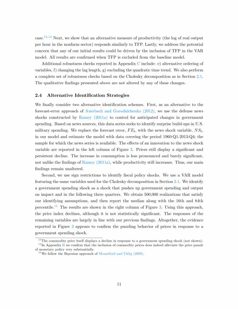
2.4 Alternative Identification Strategies

We finally consider two alternative identification schemes. First, as an alternative to the

forecast-error approach of Auerbach and Gorodnichenko (2012), we use the defense news

shocks constructed by Ramey (2011a) to control for anticipated changes in government

spending. Based on news sources, this data series seeks to identify surprise build-ups in U.S.

military spending. We replace the forecast error, FEt, with the news shock variable, NSt,

in our model and estimate the model with data covering the period 1960:Q1-2013:Q4; the

sample for which the news series is available. The effects of an innovation to the news shock

variable are reported in the left column of Figure 3. Prices still display a significant and

persistent decline. The increase in consumption is less pronounced and barely significant,

not unlike the findings of Ramey (2011a), while productivity still increases. Thus, our main

findings remain unaltered.

Second, we use sign restrictions to identify fiscal policy shocks. We use a VAR model

featuring the same variables used for the Cholesky decomposition in Section 2.1. We identify

a government spending shock as a shock that pushes up government spending and output

on impact and in the following three quarters. We obtain 500,000 realizations that satisfy

our identifying assumptions, and then report the median along with the 16th and 84th

percentile.15 The results are shown in the right column of Figure 3. Using this approach,

the price index declines, although it is not statistically significant. The responses of the

remaining variables are largely in line with our previous findings. Altogether, the evidence

reported in Figure 3 appears to confirm the puzzling behavior of prices in response to a

government spending shock.

13The commodity price itself displays a decline in response to a government spending shock (not shown).14 In Appendix B we confirm that the inclusion of commodity prices does indeed alleviate the price puzzle

of monetary policy very substantially.15We follow the Bayesian approach of Mountford and Uhlig (2009).

11

Ramey

0 5 10 15 20 25 30 35 40­2

0

2

4

Gov

.Spe

ndin

g

0 5 10 15 20 25 30 35 40­2

0

2

4

Out

put

0 5 10 15 20 25 30 35 40­2

0

2

4

Priv

ateC

ons.

0 5 10 15 20 25 30 35 40­10

0

10

20

Taxe

s

0 5 10 15 20 25 30 35 40­4

­3

­2

­1

0

1

PCE

Inde

x

0 5 10 15 20 25 30 35 40­250

­150

0

150

Int.R

ate

0 5 10 15 20 25 30 35 40­1

0

1

2

TFP

Sign Restrictions

0 5 10 15 20 25 30 35 40­2

0

2

4

0 5 10 15 20 25 30 35 40­2

0

2

4

0 5 10 15 20 25 30 35 40­2

0

2

4

0 5 10 15 20 25 30 35 40­10

0

10

20

0 5 10 15 20 25 30 35 40­2

­1

0

1

0 5 10 15 20 25 30 35 40­100

­50

0

50

100

150

0 5 10 15 20 25 30 35 40­1

0

1

2

Figure 3: The dynamic effects of a shock to government spending. Left column: Estimatesobtained using the identification scheme based on the defense news shocks of Ramey (2011a).The black line denotes the estimated response, while the grey areas represent 68 percentconfidence bands. Right column: Estimates obtained using sign restrictions. The black linedenotes the estimated response, while the grey areas represent 68 percent credible sets.

12

3 The Model

We consider a version of the baseline New Keynesian model without capital, as in Galí

(2015). A representative household works, saves, consumes, and owns the firms in the

economy. The production side consists of an intermediate goods sector operating under

imperfect competition and subject to price rigidities, and a perfectly competitive final goods

sector. A central bank conducts monetary policy, and a fiscal authority makes decisions

about changes in government spending. A key feature of the model is the presence of

variable utilization of the available technology level, as in Bianchi et al. (2017).16

3.1 The Household

The representative household maximizes expected discounted lifetime utility E0∑∞

t=0 βtUt,

where the period utility function is given by:

Ut =

C1−σt1−σ −

ψN1+ϕt

1+ϕ , σ 6= 1,

logCt − ψN1+ϕt

1+ϕ , σ = 1,

with Ct and Nt denoting non-durable consumption and labor. β ∈ (0, 1) is the discount

factor, σ > 0 is the coeffi cient of relative risk aversion, ϕ > 0 is the inverse of the Frisch

elasticity of labor supply, and ψ > 0 is the weight of labor disutility. Utility maximization

is subject to the following budget constraint:

Ct +Rt−1bt−1

πt= wtNt + bt + dt − tt,

where πt ≡ PtPt−1

is the rate of inflation in the price of consumption goods Pt, bt denotes

one-period risk-free bonds at the nominal interest rate Rt, wt is the real wage, dt is real

profits from firms, and tt is a lump-sum tax. The household chooses Ct, Nt, and bt, and the

associated first-order conditions can be stated as:

ψNϕt = wtC

−σt , (2)

C−σt = βEtRtC

−σt+1

πt+1. (3)

16The model of Bianchi et al. (2017) features endogenous variations in TFP due to variable technologyadoption and R&D investments in “knowledge capital”. Given our focus on the business-cycle effects ofchanges in fiscal policy, we abstract from the latter, as Bianchi et al. (2017) find that it plays virtually norole at business-cycle frequencies.

13

3.2 Final Goods Producers

There is a perfectly competitive sector of final goods producers, who purchase goods from

different intermediate goods producers, bundle them together, and sell them to the house-

hold or the government. Final goods producers have the following production function:

Yt =

(∫ 1

0Yt (i)

ε−1ε di

) εε−1

, ε > 1,

where Yt is aggregate production of the final good, and Yt (i) denotes the amount produced

by individual firm i in the intermediate goods sector. The cost-minimization problem of the

representative final goods firm gives rise to the following demand for intermediate good i:

Yt (i) =

(Pt (i)

Pt

)−εYt, (4)

where Pt (i) is the price of good i, and where ε thus represents the elasticity of substitution

between different intermediate goods.

3.3 Intermediate Goods Producers

There is monopolistic competition in the intermediate goods sector. Individual firm i pro-

duces according to the following production function:

Yit = VitN1−αit , (5)

where 0 ≤ α < 1, so as to allow for decreasing or constant returns to scale in labor. Nit is

the amount of labor hired by firm i, and Vit is the level of utilized technology. In turn, this

is given by:

Vit = uitAt, (6)

where uit denotes the firm-specific utilization rate, and At is the economy-wide and exoge-

nous level of technology, which grows deterministically at the rate λA ≥ 0:

At = (1 + λA)At−1. (7)

We let each firm decide on the rate at which it wishes to utilize the available technology in

society. As in Bianchi et al. (2017), technology utilization may be interpreted as a measure

of the capacity of the firm to adopt new knowledge or inventions into the production setup.

As new inventions arrive, each firm needs to exert an effort to internalize this new technology.

By endogenizing the rate of technology adoption, we allow firms to choose when to make

14

this effort, subject to an adjustment cost whenever uit differs from its steady-state level

u. We thus assume that it is costly for a firm to fully adopt new inventions into their

production process as they arrive, for example because employees must be trained in using

the new technology. We let the function z (uit) denote the adjustment costs associated

with the choice of uit. As in Bianchi et al. (2017), this function satisfies z (u) = 0, i.e.,

adjustment costs are zero in steady state. We also require z′ (u) > 0 and z′′ (·) > 0. Further,

in line with the literature on variable utilization of capital (e.g., Christiano et al., 2005), we

assume that u = 1. As we shall see, this choice pins down z′ (1). The curvature parameter

z′′ (·) measures how quickly adjustment costs rise with changes in the rate of technology

utilization.17

Each firm chooses labor inputs Nit and technology utilization uit so as to minimize its

costs subject to (5). This gives rise to the following first-order conditions:

wt = (1− α)mcitYitNit

, (8)

z′ (uit) = mcitYituit, (9)

where mcit is the multiplier associated with (5), and represents the real marginal cost of

production. (8) equates the real wage to the marginal product of labor, while (9) states

that the marginal cost of higher utilization, given by the increase in adjustment costs

z′ (uit), must equal the marginal product of a higher utilization rate. The utilization rate of

technology affects the marginal cost in two ways: On the one hand, a higher rate of utilization

allows the firm to increase production for given inputs of labor, effectively working like an

increase in productivity. On the other hand, higher utilization is costly. If the former effect

is suffi ciently strong, a higher utilization rate reduces the marginal cost. In response to a

government spending shock, this effect may even be strong enough to overcome the increase

in the wage rate, thus paving the way for an equilibrium decline in the marginal cost and,

as a consequence, inflation.

When setting their price, intermediate goods firms are subject to a nominal rigidity in

the form of quadratic price adjustment costs, as in Rotemberg (1982). Adjustment costs

Υit are scaled by nominal output, and take the following form:

Υit =γ

2

(PitPit−1

− 1

)2PtYt,

where γ > 0 measures how costly it is to change prices. Firm i sets its price so as to

17The only characteristic of the function z affecting the steady state is z′ (1). Moreover, as in Christianoet al. (2005), only the ratio z′′(·)

z′(1) affects the dynamics of our model outside steady state.

15

maximize profits, and this problem can be written in real terms as:

maxPit

E0∞∑t=0

qt,t+1

[(PitPt−mcit

)Yit − z (uit)−Υit

],

subject to the demand function (4). Here, qt,t+1 ≡ β Etλt+1λtis the stochastic discount factor

of the household, with λt denoting the marginal utility of consumption. Upon deriving the

first-order condition, we impose a symmetric equilibrium in which all firms charge the same

price, allowing us to state the optimality condition as:

1− ε+ εmct = γ (πt − 1)πt − γEtqt,t+2qt,t+1

(πt+1 − 1)Yt+1Yt

πt+1. (10)

This condition can be written on log-linearized form as a New Keynesian Phillips Curve.

3.4 Monetary and Fiscal Policy

Fiscal policy is assumed to follow a balanced-budget rule:

gt = tt, (11)

where government spending, gt, satisfies:

log gt = (1− ρG) g + ρG log gt−1 + εGt , (12)

with the innovation εGt following an i.i.d. normal process with standard deviation σG, and

where g denotes government spending in steady state, while ρG ≥ 0 is the persistence of

the shock.

The monetary policy rule is specified as follows:

iti

=(πtπ

)φπ (YtY

)φy, (13)

where φπ > 1 and φy ≥ 0 denote the policy responses to inflation and output deviations

from steady state, respectively, with π and Y denoting the steady-state levels of inflation

and output.

3.5 Market Clearing

Bonds are in zero net supply:

bt = 0. (14)

16

The labor market clears when: ∫ 1

0Nitdi = Nt. (15)

Finally, goods market clearing requires:

Yt − z (uit)−Υit = Ct + gt. (16)

When solving the model, we detrend all variables to eliminate the trend growth in the level

of technology. Considering only symmetric equilibria in which all firms make the same

decisions allows us to discard subscript i’s. We then log-linearize the equilibrium conditions

around the non-stochastic steady state of the model, which is described in Appendix D.1.

The log-linearized equilibrium conditions are presented in Appendix D.2.

4 Analytics of the Model

To build intuition on the ability of the model to reproduce our empirical findings– in par-

ticular, a decline in inflation and an increase in consumption in response to expansionary

fiscal policy– we find it useful to offer some analytical insights. To this end, we make the

following simplifying assumptions, all of which are regularly encountered in the existing

business-cycle literature: We assume constant returns to scale in production (α = 0), log

utility in consumption (σ = 1), unitary (inverse) Frisch elasticity of labor supply (ϕ = 1),

no monetary policy reaction to the output gap (φy = 0), and a constant level of technology

(At = 1, ∀t). Under these conditions, the log-linearized version of the model can be reducedto two equations in consumption and inflation (plus an exogenous process for government

spending), as we show in Appendix D.3. In fact, letting xt denote the (log) deviation of a

generic variable xt from its steady-state value x, these two equations can be stated as (see

Appendix D.3 for details):

− Ct = Et(−Ct+1 + φππt − πt+1

), (EE)

πt = βEtπt+1 + aCt − bgt, (NKPC)

where a, b are functions of the deep parameters of the model. We provide necessary and

suffi cient conditions below for a and b to be strictly positive. (EE) simply combines the

household’s Euler equation with the monetary policy rule, while (NKPC) emerges by sub-

stitution of the remaining equilibrium conditions into the New Keynesian Phillips Curve.

In Figure 4, we provide a graphical representation of the model (EE)-(NKPC) in (Ct, πt)-

space. (EE) can be represented by a downward-sloping line (this can be seen most clearly

in the case of non-persistent shocks, in which case EtCt+1 = Etπt+1 = 0), whereas (NKPC)

17

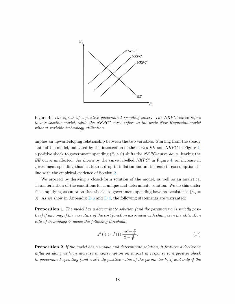
Figure 4: The effects of a positive government spending shock. The NKPC’-curve refersto our baseline model, while the NKPC”-curve refers to the basic New Keynesian modelwithout variable technology utilization.

implies an upward-sloping relationship between the two variables. Starting from the steady

state of the model, indicated by the intersection of the curves EE and NKPC in Figure 4,

a positive shock to government spending (gt > 0) shifts the NKPC -curve down, leaving the

EE curve unaffected. As shown by the curve labelled NKPC’ in Figure 4, an increase in

government spending thus leads to a drop in inflation and an increase in consumption, in

line with the empirical evidence of Section 2.

We proceed by deriving a closed-form solution of the model, as well as an analytical

characterization of the conditions for a unique and determinate solution. We do this under

the simplifying assumption that shocks to government spending have no persistence (ρG =

0). As we show in Appendix D.3 and D.4, the following statements are warranted:

Proposition 1 The model has a determinate solution (and the parameter a is strictly posi-tive) if and only if the curvature of the cost function associated with changes in the utilization

rate of technology is above the following threshold:

z′′ (·) > z′ (1)mc− g

Y

2− gY

. (17)

Proposition 2 If the model has a unique and determinate solution, it features a decline ininflation along with an increase in consumption on impact in response to a positive shock

to government spending (and a strictly positive value of the parameter b) if and only if the

18

curvature of the cost function is below the following threshold:

z′′ (·) < z′ (1) . (18)

Proof. See Appendix D.3 and D.4.Note that the steady-state value of mc is given by mc = ε−1

ε < 1. This means that there

always exists a range of values for z′′ (·) for which both (17) and (18) are satisfied. Ourbaseline calibration of the next section implies mc = 5

6 ,gY = 0.245, and z′ (1) = 0.21. These

values produce an admissible range of z′′ (·) ∈ [0.07, 0.21]. For all values within this range,

the model has a determinate equilibrium featuring a drop in inflation and an increase in

consumption on impact.

We can explain these requirements as follows: (18) requires that the curvature z′′ (·)cannot be too large. If z′′ (·) is very high, changes to the utilization rate are very costly, sofirms will be hesitant to make such changes. In the limiting case of z′′ (·) → ∞, firms willchoose to never adjust the utilization rate, which will therefore remain constant, exactly

as in a model without an endogenous utilization rate. Indeed, we show in Appendix D.5

that for z′′ (·) → ∞, the analytical solution to our model collapses to that of a basic NewKeynesian model, and that the latter always implies an increase in inflation– driven by

the upward movement in the wage rate– along with a decline in consumption when gt

increases. Graphically, this implies that the NKPC -curve is shifted up, as illustrated by the

curve labelled NKPC” in Figure 4.18 To overturn this, and ensure a positive value of b and

a downward shift in the NKPC -curve in Figure 4, it is crucial that the utilization rate is

suffi ciently responsive, which in turn requires a limited cost of adjusting it.

Conversely, (17) provides a lower bound on the adjustment cost, effectively entailing that

the rate of technology utilization cannot be too responsive. If this condition is not met,

the model does not have a determinate solution. Intuitively, if the costs associated with

changing the utilization rate are suffi ciently small, the optimal utilization rate may tend to

infinity in response to an expansionary shock. Thus, the adjustment cost function needs to

display a certain degree of curvature for the costs to increase suffi ciently with the utilization

rate and contain the movements in the latter. In terms of the graphical representation in

Figure 4, (17) ensures an upward-sloping NKPC -curve, which is necessary for the model to

have a determinate equilibrium.19

18The basic New Keynesian model– subject to the same parameter restrictions as our model– featuresan Euler equation identical to (EE), and a rewritten New Keynesian Phillips Curve of the same form as(NKPC), but where the coeffi cient in front of gt is strictly negative. See Appendix D.5 for details.19 Interestingly, this type of constraint does not arise in models featuring variable utilization of the capital

stock. In those models, adjustment costs will be tied to the rental rate of capital in equilibrium: capitalproducers will never find it optimal to raise the utilization rate to a level at which the associated adjustmentcosts outweigh the rental rate earned on utilized capital (see, e.g., Smets and Wouters, 2007). In our setup,instead, the utilization decision regards a production “factor”which is intrinsically free to use; the level of

19

The analysis above establishes some general conditions under which our model is able to

generate impact multipliers in line with the empirical evidence from Section 2. Effectively,

our mechanism works much like an increase in the level of technology– in fact, it produces

an increase in measured TFP (Vt), as we shall see below. The decline in marginal costs

induces firms to reduce their prices, thus generating a decline in inflation. The central

bank responds by reducing the nominal and real interest rate, thus facilitating an increase

in consumption. In fact, in our simple environment, this is necessary and suffi cient to

generate an increase in private consumption. Again, this can be seen most easily in the case

of non-persistent shocks, in which case (EE) simply states that consumption equals minus

the nominal (and real) interest rate (in deviations from steady state). More generally, these

insights carry over to the next section, where we lift some of the simplifying assumptions

made in this section and resort to numerical analyses of the quantitative implications of our

model.20

5 Dynamic Effects of a Government Spending Shock

In this section, we use model simulations to study the effects of a government spending

shock beyond the quarter in which the shock hits the economy. To this end, we assign

realistic values to all parameters of the model, and study the implied impulse responses.

We also offer a set of sensitivity checks regarding certain key parameters.

5.1 Calibration

The baseline calibration of the model is as follows: We set β = 0.99, implying an annualized

real interest rate of 4% in steady state. We set the deterministic growth rate of technology

to λA = 0 for simplicity. The coeffi cient of relative risk aversion is set to σ = 2, in line

with microeconometric estimates (see, e.g., Attanasio and Weber, 1995). As in Christiano

et al. (2005), we maintain the assumption from the previous section of an (inverse) Frisch

elasticity of labor supply of unity; ϕ = 1. This value represents a compromise between

microeconometric studies– where 1 can be regarded as an upper bound; see Chetty et al.

(2011)– and macroeconomic models, where values above 1 are not uncommon (see, e.g.,

technology in society. The only cost of utilizing technology comes from the adjustment costs, motivatingthe presence of a lower bound on these.20A final insight can be obtained from the simple model above: If we were to introduce a monetary policy

shock into the model, the shock would appear in (EE), but not in (NKPC). A contractionary monetarypolicy shock would shift the EE -curve down along the NKPC -curve, generating a decline in inflation. Inother words, our model is not able to account for the “price puzzle”of monetary policy (Sims, 1992). Thereason is that a government spending shock affects natural (i.e., flexible-price) output via its effect on laborsupply, and thus exerts a direct effect on inflation, whereas a monetary policy shock leaves natural outputunaffected.

20

Hall, 2009). The weight on disutility of labor hours in the utility function, ψ, is calibrated

so that N = 1/4 (this only affects the scale of the economy). On the production side, we

follow most of the literature and set ε = 6, implying a steady-state markup of 20 percent.

We maintain the assumption of constant returns to scale (α = 0) in our baseline analysis,

and then study the case of decreasing returns to scale in Section 5.3.3. The adjustment

cost associated with price changes is calibrated so that a given price is changed, on average,

every 3 quarters, consistent with microeconometric evidence reported by Nakamura and

Steinsson (2008). Given the other parameters, this implies a value of γ = 29.41.

Regarding the policy-related parameters, we follow most of the literature in setting

the steady-state inflation rate to zero. The response of monetary policy to movements in

inflation is set to a standard value of φπ = 1.5 (see, e.g., Taylor, 1993). We initially set the

output response to zero, φy = 0, and then “switch on”this reaction when studying the role

of monetary policy in Section 5.3.2. The persistence of government spending shocks is set

to ρG = 0.9, in line with Galí et al. (2007). The ratio of government spending to output in

the model matches the sample average in the data for the period 1960-2017, which equalsgY = 0.245.

Finally, we need to specify and parametrize the functional form of the adjustment cost

associated with changes in the technology utilization rate. We assume that adjustment

costs are given by:21

z (ut) = χ1 (ut − u) +χ22

(ut − u)2 , (19)

where χ1, χ2 > 0, and where u = 1 again denotes the steady-state level of ut. This implies

that z′ (ut) = χ1 + χ2 (ut − u). As already described, we calibrate the value of z′ (1) = χ1

to ensure that the rate of utilization equals 1 in steady state. This returns a value of

χ1 = 0.21. The curvature parameter z′′ (·) = χ2 is harder to pin down. Conditional on our

baseline calibration of all other parameters, the admissible range of values for this parameter

established analytically in Section 4 changes slightly: For any value of χ2 ∈ [0.03, 0.21], we

obtain impact effects of inflation and consumption in line with the data. In the simulations

below, we pick a baseline value of χ2 = 0.1, while our robustness checks shed more light on

the quantitative importance of this parameter.

5.2 Impulse-Response Analysis

Given our baseline calibration, Figure 5 displays the impulse responses of the model to a

government spending shock of 1 percent (solid blue lines), along with the responses of a basic

New Keynesian model without variable technology utilization (dashed red lines). As the

21This functional form satisfies the requirements stated by Bianchi et al. (2017) and is consistent with thestandard specification of capital adjustment costs in the literature; e.g. in Christiano et al. (2005).

21

figure illustrates, our baseline model implies an increase in the rate of technology utilization

in response to the shock. This is suffi cient to generate a decline in marginal costs, despite

the increase in the wage rate. As a consequence, inflation drops. This leads to a reduction

in the nominal interest rate, reducing also the real rate. In line with the intuition traced out

in the previous section, consumption therefore increases, in turn amplifying the increase in

total output. The negative response of the nominal interest rate is in line with the empirical

evidence from Section 2.22 Also in line with the data, we observe an increase in “Measured

TFP”as given by the utilized technology level, Vt. In the absence of exogenous technology

shocks, this variable moves one-for-one with the utilization rate. In contrast, measured

TFP remains constant in the model without variable technology utilization. In that case

marginal costs increase in response to the shock, generating an increase in inflation and the

nominal interest rate, and a drop in consumption, in contrast to our empirical evidence.

The government spending multiplier on total value added (defined as the sum of private

and public consumption) is substantially higher in our baseline model (1.30) than in the

model without variable technology utilization (0.75).

5.3 Sensitivity Analysis

This subsection explores the robustness of our findings with respect to some of our key

parameter values and modeling choices.

5.3.1 Movements in the Technology Utilization Rate

Given the uncertainty surrounding the cost of changing the rate of technology utilization,

it is worth pointing out that we do not require dramatic changes in the utilization rate to

obtain a decline in inflation: Under our baseline calibration, the utilization rate increases

by less than 0.5 percent; somewhat less than the increase in output. This is similar to the

behavior of the utilization rate of capital in Christiano et al. (2005), which moves slightly less

than 1-for-1 with output in the data and in their model. To shed some additional light on the

robustness of our findings, the dotted green lines in Figure 5 show the corresponding impulse

responses after changing the value of χ2 from 0.1 to 0.15. In this case, the utilization rate

increases only by around 0.3 percent on impact. Yet, inflation and consumption still behave

in accordance with the empirical evidence, but now display much smaller changes. This

shows that even relatively small movements in the utilization rate are suffi cient to obtain

the desired responses from the model. While data on technology utilization is not readily

22Additionally, the positive response of the wage rate, as well as that of labor hours (not reported), whilenot included in our VAR model, are in line with existing empirical evidence. Among others, Galí et al. (2007)and Andres et al. (2015) report that wages and hours both rise in response to an increase in governmentspending.

22

10 20 30 400

0.5

1

1.5Government Spending

10 20 30 40­0.05

0

0.05Inflation

10 20 30 40

­0.1

0

0.1

Consumption

10 20 30 400

0.5

1 Total Output

10 20 30 40

­0.05

0

0.05

Nominal Interest Rate

10 20 30 400

0.2

0.4

0.6Technology Utilization

10 20 30 400

0.2

0.4

0.6Wage

10 20 30 40

­0.02

0

0.02

Marginal Cost

10 20 30 400

0.2

0.4

0.6Measured TFP

Baseline model NK model 2 = 0.15

Figure 5: Impulse responses of key variables to a positive government spending shock of 1percent. Solid blue lines: baseline model with χ2 = 0.1. Dashed red lines: model withoutvariable technology utilization (obtained by setting χ2 = 100). Dotted green lines: baselinemodel with alternative value of χ2 = 0.15.

available, Bianchi et al. (2017) argue that their model-implied rate of technology utilization

is closely correlated with data on the software expenditures of firms; one potential measure

of technology adoption. We have verified that this correlation also emerges conditional on

a government spending shock: When we include software expenditures in our baseline VAR

model of Section 2, we observe a significant increase in this variable after an increase in

government spending (see Figures C.7-C.8 in Appendix C).

5.3.2 The Role of Monetary Policy

The stance of monetary policy plays a key role in the transmission of fiscal policy. At the

heart of the negative relationship between inflation and consumption implied by our baseline

model are movements in the real interest rate: In the simplified model version studied in

Section 4, consumption increases if and only if the central bank engineers a decline in the

real interest rate upon observing a drop in inflation. This, in turn, requires a suffi ciently

strong reaction of the nominal policy rate to a given change in inflation. When we allow for

a monetary policy reaction to output fluctuations, this direct link between consumption and

inflation breaks down. In terms of the graphical representation in Figure 4, the (EE)-curve

becomes steeper and is shifted down in response to a positive government spending shock.

23

10 20 30 400

0.5

1

1.5Government Spending

10 20 30 40­0.15

­0.1

­0.05

0Inflation

10 20 30 400

0.05

0.1

Consumption

10 20 30 400

0.5

1Output

10 20 30 40

­0.1

­0.05

0Interest Rate

10 20 30 400

0.2

0.4

0.6Technology Utilization

10 20 30 400

0.2

0.4

0.6Wage

10 20 30 40­0.1

­0.05

0Marginal Cost

10 20 30 400

0.2

0.4

0.6Measured TFP

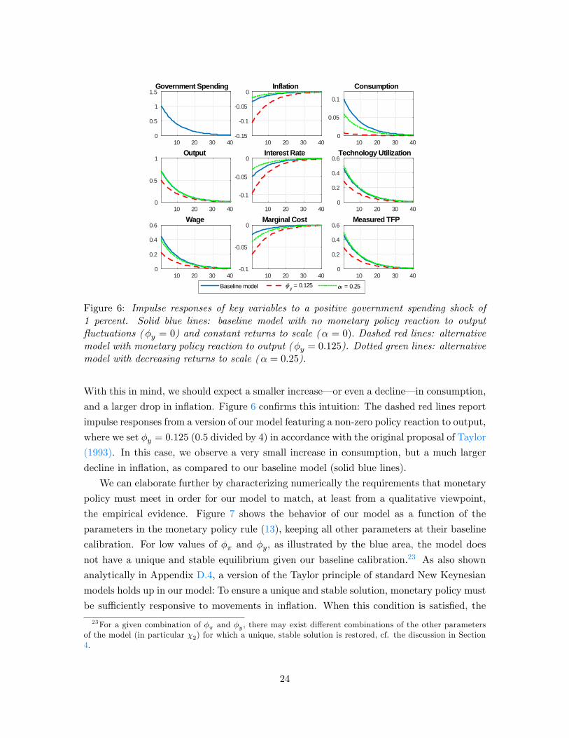
Baseline model y = 0.125 = 0.25

Figure 6: Impulse responses of key variables to a positive government spending shock of1 percent. Solid blue lines: baseline model with no monetary policy reaction to outputfluctuations (φy = 0) and constant returns to scale (α = 0). Dashed red lines: alternativemodel with monetary policy reaction to output (φy = 0.125). Dotted green lines: alternativemodel with decreasing returns to scale (α = 0.25).

With this in mind, we should expect a smaller increase– or even a decline– in consumption,

and a larger drop in inflation. Figure 6 confirms this intuition: The dashed red lines report

impulse responses from a version of our model featuring a non-zero policy reaction to output,

where we set φy = 0.125 (0.5 divided by 4) in accordance with the original proposal of Taylor

(1993). In this case, we observe a very small increase in consumption, but a much larger

decline in inflation, as compared to our baseline model (solid blue lines).

We can elaborate further by characterizing numerically the requirements that monetary

policy must meet in order for our model to match, at least from a qualitative viewpoint,

the empirical evidence. Figure 7 shows the behavior of our model as a function of the

parameters in the monetary policy rule (13), keeping all other parameters at their baseline

calibration. For low values of φπ and φy, as illustrated by the blue area, the model does

not have a unique and stable equilibrium given our baseline calibration.23 As also shown

analytically in Appendix D.4, a version of the Taylor principle of standard New Keynesian

models holds up in our model: To ensure a unique and stable solution, monetary policy must

be suffi ciently responsive to movements in inflation. When this condition is satisfied, the

23For a given combination of φπ and φy, there may exist different combinations of the other parametersof the model (in particular χ2) for which a unique, stable solution is restored, cf. the discussion in Section4.

24

Figure 7: Model outcomes for different combinations of monetary policy parameters. Bluearea: No unique and determinate solution. Yellow area: The model fails to generate adecline in inflation and/or an increase in consumption on impact. Green area: The modelgenerates a decline in inflation and an increase in consumption on impact. The black dotindicates our baseline calibration.

ratio φπφymust be suffi ciently high to ensure that the model produces the desired responses.

The green area indicates combinations of policy parameters for which the model produces

an increase in consumption and a decline in inflation on impact, while the yellow area

indicates combinations where either of these does not obtain. The black dot denotes our

baseline calibration. For relatively high values of φπ, the decline in inflation associated with

an increase in government spending leads to a reduction in the nominal and real interest rate,

and thus an increase in consumption. Given the empirical evidence presented in Section 2,

this case appears to be the most realistic.

5.3.3 Decreasing Returns to Scale

So far in our analysis, we have assumed a constant-returns-to-scale technology in the in-

termediate goods sector. This assumption facilitates a decline in inflation. If instead there

are decreasing returns to scale (α > 0), a given increase in production requires a larger

increase in labor inputs, thus driving up marginal costs, which– all else equal– makes it

harder to observe a decline in marginal costs in equilibrium. It is therefore important to

verify that our proposed mechanism can reproduce the empirical evidence even in the case

of decreasing returns to scale. To this end, the dotted green lines in Figure 6 show impulse

responses from our model under the assumption that α = 0.25, as in Galí (2015), while the

25

solid blue lines display our benchmark model for comparison.24 As can be seen, our main

findings are confirmed, as the model is still able to generate a drop in inflation alongside an

increase in consumption. However, from a quantitative viewpoint, the movements in these

variables are somewhat smaller than those observed in our baseline model, reflecting that

our mechanism of variable technology adoption has less quantitative bite in this case.

6 An Estimated Model with Capital Formation

The final step of our analysis is to evaluate the quantitative performance of our proposed

mechanism in an estimated model of the U.S. economy. To this end, we augment the model

with physical capital formation in order to make it more realistic and thus appropriate

for estimation. We also introduce habit formation in consumption to enable our model

to reproduce the hump-shaped response of private consumption observed in our empirical

analysis. In this section, we first describe the details of these model extensions, and then

turn to the estimation of the model.

6.1 A Model with Capital and Habit Formation

We assume that the capital stock is owned by the household and rented to intermediate

goods producers in each period. This means that the household makes the choices related

to capital accumulation, while the firms choose how much capital to employ in production.

The law of motion for capital is given by:

Kt = (1− δ)Kt−1 +

[1− κ

2

(ItIt−1

− 1

)2]It, (20)

where Kt and It denote the stock of capital and the investment in new capital, 0 ≤ δ < 1 is

the rate at which capital depreciates, while κ > 0 denotes quadratic investment adjustment

costs. The budget constraint of the household now incorporates investment expenses and

rental income from capital (with rKt denoting the rental rate):

Ct + It +Rt−1bt−1

πt= wtNt + rKt−1Kt−1 + bt + dt − tt. (21)

24 In this experiment, we have again set φy = 0 as in the baseline model. The calibrated parameters ψ, γ,and χ1 are automatically adjusted so as to ensure that our calibration targets are maintained.

26

In the presence of internal habit formation in consumption, the utility function of the

representative household becomes:

E0

∞∑t=0

βt

[(Ct − θCt−1)1−σ

1− σ − ψN1+ϕt

1 + ϕ

], σ 6= 1,

where 0 ≤ θ < 1 is the degree of habit formation. The first-order conditions for the choices

of consumption, labor, and bond holdings can be stated as:

λt = (Ct − θCt−1)−σ − βθ (EtCt+1 − θCt)−σ , (22)

ψNϕt

wt= λt, (23)

λt = βEtRtλt+1πt+1

, (24)

with λt denoting the multiplier associated with (21). We can use (22) to substitute for λt in

(23) and (24), thus obtaining two conditions to replace (2) and (3) in our extended model.

In addition, the household now also chooses investment It and capital Kt, subject to (20)

and (21). The relevant first-order conditions can be written as:

1 = Qt

(1− κ

2

(ItIt−1

− 1

)2− κ

(ItIt−1

− 1

)ItIt−1

)

+βEtQt+1λt+1

λtκ

(It+1It− 1

)I2t+1I2t

, (25)

βEtλt+1[rKt + (1− δ)EtQt+1

]= λtQt, (26)

where Qt denotes the price of installed capital (in units of consumption), which is given

by Qt ≡ µtλt, where µt is the multiplier associated with (20). Note that (24) and (26) can

be combined to yield the following arbitrage condition relating the expected real return on

capital to that on bonds:rKt + (1− δ)EtQt+1

Qt=

RtEtπt+1

.

Production is now given by:

Yit = VitN1−αit Kα

it−1, (27)

and the cost-minimization problem of each intermediate goods producer yields the following

first-order condition for the demand for capital:

rKt = αEtmcit+1EtYit+1Kit

, (28)

27

while the first-order conditions for labor and for technology utilization are still given by (8)

and (9). The aggregate resource constraint now reads:

Yt = Ct + It + gt + z (ut) +γ

2(πt − 1)2 Yt. (29)

This completes the description of our extended model. We present the steady state and the

log-linearization of this model in Appendix D.6.

6.2 Estimation Strategy

The model is estimated using indirect inference. Following Christiano et al. (2005) among

others, we estimate (a subset of) the parameters of the model by matching the model-implied

impulse responses to a government spending shock to the empirical responses presented in

Figure 2. To this end, we first split the parameters into two groups. ω1 =α, β, ε, χ1, ψ,

gY

contains the parameters that we choose to calibrate. We maintain the same parameter values

and calibration targets as described in Section 5.1, as well as α = 0.25 as in Section 5.3.3.

We then collect in ω2 =γ, δ, θ, κ, ρG, σ, ϕ, φπ, φy, χ2

the parameters to be estimated. Let

Λ (ω2) denote the model-implied impulse responses, which are functions of the parameters,

while Λ denotes the corresponding empirical estimates from our VAR model. We obtain

the vector of parameter estimates ω2 by solving:

ω2 = arg minω2

(Λ (ω2)− Λ

)′W(

Λ (ω2)− Λ). (30)

The weighting matrix W is a diagonal matrix with the sample variances of the VAR-based

impulse responses along the diagonal. Effectively, this means that we are attaching higher

weights to those impulse responses that are estimated most precisely. We match impulse

responses for the seven variables reported in Figure 2 plus investment, which we now include

in our structural VAR model, using the responses during the first 20 quarters after the

shock. In addition to the intervals over which they are defined, we impose few bounds on

the estimated parameters, as discussed in the next subsection.25

6.3 Estimation Results

We report the estimated parameter values in Table 2, as well as the associated standard

errors, which are computed using an application of the delta method, as described, e.g.,

in Hamilton (1994). We first note that all parameters take on values that are generally in

25Since the vector of estimated parameters includes both the parameters in the monetary policy rule(φπ and φy) and the curvature of the utilization cost function (χ2), our estimation procedure sometimesdraws parameter vectors for which the model has no determinate solution. To circumvent this problem, weintroduce a penalty function that drives the procedure away from such cases.

28

line with the existing literature. The estimated cost of adjusting prices implies an average

lifetime of a given price of around 412 quarters.26 The depreciation rate of capital and the

degree of habit formation are similar to those found in most studies. The estimated invest-

ment adjustment cost parameter is modest, although available estimates of this parameter

display substantial variation. The persistence of the government spending shock is relatively

high. Regarding the estimate of ϕ, we note that it almost reaches the lower bound of 1/5

that we impose in order to avoid a Frisch elasticity of labor supply above 5. As discussed

in Section 5.1, while this value is too high according to microeconometric studies, it is not

uncommon in the Real Business Cycle literature. The estimated coeffi cient of risk aversion

is relatively low in order to facilitate a sizable increase in consumption in response to the

observed drop in the interest rate. The parameters of the monetary policy rule imply a pre-

dominance of inflation over output gap stabilization. The estimate of φy is almost driven to

its lower bound of zero in order to enable the model to produce an increase in private con-

sumption, cf. Section 5.3.2. Finally, given its central role in our model, the estimated value

of χ2 is of particular interest. We obtain a parameter estimate of χ2 = 0.457. This value

is somewhat higher than those considered so far. Note, however, that the introduction of

capital changes the admissible range of values of χ2 for which the model has a determinate

solution featuring a decline in inflation and an increase in consumption on impact. Given

the remaining parameter estimates, this result obtains for all values of χ2 ∈ [0.457; 0.875],

with the estimation procedure selecting a value of χ2 at the lower bound of this range in

order to generate a substantial increase in consumption.

We turn next to the estimated impulse-response functions from the model, which are

reported in Figure 8 alongside their empirical counterparts from the VAR model.27 Several

things are noteworthy. First, the estimated DSGE model matches the responses of all

variables qualitatively. Second, the quantitative performance of the model is satisfactory

for most variables. The model-implied increase in consumption and the decline of the

interest rate fall short of our VAR evidence.28 With the exception of net tax revenues, the

remaining variables are generally in line with the data.29

26With decreasing returns to labor inputs, the mapping between the value of γ and the duration of a givenprice is different from the one in our basic model with constant returns to scale calibrated in Section 5.1.See also Galí (2015).27The model-implied impulse response of the price level is computed as the cumulative sum of the response

of inflation.28This suggests that our proposed mechanism might successfully combine with existing methods to gen-

erate a more sizable increase in private consumption, such as the rule-of-thumb households of Galí et al.(2007).29The response of taxes is substantially smaller than in the VAR model. However, matching the response of

tax revenues would require a more thorough treatment of public finances than warranted by our assumptionof a balanced government budget each period. In the context of our estimation, the wide confidence band ofthe VAR-based response of taxes implies that this variable receives a low weight in the estimation procedure.

29

Table 2: Parameter Estimates

Parameter Estimate

γ 232.495(19.389)

δ 0.034(0.023)

θ 0.582(0.457)

κ 1.930(0.981)

ρG 0.962(0.001)

σ 0.555(0.938)

ϕ 0.211(0.399)

φπ 1.276(0.816)

φy 0.010(0.033)

χ2 0.457(0.101)

Notes: We report standard errors in brackets, obtained using the delta method.

In particular, the response of the price level is usually within the estimated confidence

band from the VAR model. This confirms the ability of our model to generate a drop

in prices of a realistic magnitude. The DSGE model slightly overestimates the increases

in output and TFP in the first year after the shock. Notably, we observe an increase in

investment in the DSGE model as well as in the VAR model. In the former, this finding

is driven by increases in labor supply and technology utilization in combination with the

reduction in the nominal interest rate.30 Finally, while the response of technology utilization

is not matched to any empirical counterpart, we note that the utilization rate again increases

somewhat less than 1-for-1 with output, as discussed in Section 5.3.1.

30Regarding the VAR evidence, Furlanetto (2011) points out that the empirical literature has produced nofirm consensus on the response of investment to government spending shocks, and that the response tendsto differ across identification schemes. Indeed, when we include investment in our Cholesky VAR model, theresponse becomes negative.

30

48

1216

20

0

0.51

1.5

Gov

ernm

ent S

pend

ing

VAR

evid

ence

Estim

ated

DSG

E m

odel

48

1216

20

0

0.51

1.5

Out

put

48

1216

20

0

0.51

1.5

Cons

umpt

ion

48

1216

20

02468Ta

xes

48

1216

20­1

­0.8

­0.6

­0.4

­0.20

0.2

Pric

e le

vel

48

1216

20­1

00­50050

Inte

rest

Rat

e

48

1216

20­0

.25

00.250.5

0.75

TFP

48

1216

20­2­10123

Inve

stm

ent

48

1216

200.

1

0.150.

2

0.250.

3

0.350.

4Ut

iliza

tion

Figure8:Impulseresponsestoagovernmentspendingshockof1percent.Solid

blacklines:estimatedVARmodelusingthe

identificationbasedonforecasterrors.Greyareas:68percentconfidencebandsfrom

theVARmodel.Dottedbluelines:estimated

DSGEmodel.

31

7 Conclusion

The assumption that increases in government spending are inflationary is a key building

block of many theoretical accounts of fiscal policy. However, this paper presents empirical

evidence that inflation tends to drop in response to increases in government spending in

the U.S. economy. This result is robust across a wide range of empirical specifications. It

emerges alongside the increase in output and private consumption documented in previous

studies, as well as an increase in TFP.

To account for our results, we propose a model of variable technology utilization in the

spirit of Bianchi et al. (2017). We show that the model can replicate the observed response

of prices and other key macroeconomic variables to a government spending shock. Our

proposed mechanism may be one of several candidates that can help explain this set of

findings. In this respect, our analytical and graphical analysis has sketched some general

requirements that other candidate explanations must satisfy. In particular, accounting for

potential supply-side effects of fiscal policy seems crucial. We think of this as a fruitful

avenue for future research.

32

References

Afonso, A., and R. Sousa, 2012, The Macroeconomic Effects of Fiscal Policy, Applied

Economics 44, 4439—4454.

Aghion, P., D. Hemous, and E. Kharroubi, 2014, Cyclical Fiscal Policy, Credit Constraints,

and Industry Growth, Journal of Monetary Economics 62, 41—58.

Aghion, P., and P. Howitt, 1992, A Model of Growth Through Creative Destruction, Econo-

metrica 60, 323—351.

Anzoategui, D., D. Comin, M. Gertler, and J. Martinez, 2017, Endogenous Technology

Adoption and R&D as Sources of Business Cycle Persistence, American Economic

Journal: Macroeconomics, forthcoming.

Andrés, J., J. Boscá, and J. Ferri, 2015, Household Debt and Fiscal Multipliers, Economica

82, 1048—1081.

Attanasio, O., and G. Weber, 1995, Is Consumption Growth Consistent with Intertemporal

Optimization? Evidence from the Consumer Expenditure Survey, Journal of Political

Economy 103, 1121—1157.

Auerbach, A., and Y. Gorodnichenko, 2012, Measuring the Output Responses to Fiscal

Policy, American Economic Journal: Economic Policy 4, 1—27.

Bachmann, R., and E. Sims, 2012, Confidence and the Transmission of Government Spend-

ing Shocks, Journal of Monetary Economics 59, 235—249.

Bai, Y., J.V. Rios-Rull, and K. Storesletten, 2017, Demand Shocks as Technology Shocks,

working paper.

Barth, M., and V. Ramey, 2002, The Cost Channel of Monetary Transmission, in Bernanke,

B., and K. Rogoff (eds.), NBER Macroeconomics Annual 2001, 199—245.

Baxter, M., and R. King, 1993, Fiscal Policy in General Equilibrium, American Economic

Review 83, 315—334.

Ben Zeev, N., and E. Pappa, 2017, Chronicle of a War Foretold: The Macroeconomic Effects

of Anticipated Defense Spending Shocks, Economic Journal 127, 1568—1597.

Benigno, G., and L. Fornaro, 2017, Stagnation Traps, Review of Economic Studies, forth-

coming.

33

Bianchi, F., H. Kung, and G. Morales, 2017, Growth, Slowdowns, and Recoveries, Journal

of Monetary Economics, forthcoming.

Bilbiie, F., 2011, Non-Separable Preferences, Frisch Labor Supply, and the Consumption

Multiplier of Government Spending: One Solution to a Fiscal Policy Puzzle, Journal

of Money, Credit and Banking 43, 221—251.

Blanchard, O., and R. Perotti, 2002, An Empirical Characterization of the Dynamic Effects

of Changes in Government Spending and Taxes on Output, Quarterly Journal of

Economics 117, 1329—1368.

Burnside, C., M. Eichenbaum, and J. Fisher, 2004, Fiscal Shocks and Their Consequences,

Journal of Economic Theory 115, 89—117.

Caldara, D., and C. Kamps, 2008, What Are the Effects of Fiscal Shocks? A VAR-based

Comparative Analysis, European Central Bank Working Paper 877.

Canova, F., and E. Pappa, 2007, Price Differentials in Monetary Unions: The Role of Fiscal

Shocks, Economic Journal 117, 713—737.

Canzoneri, M., R. Cumby, and B. Diba, 2002, Should the European Central Bank and the

Federal Reserve be Concerned About Fiscal Policy?, working paper of the Federal

Reserve Bank of Kansas City’s Symposium on Rethinking Stabilization Policy.

Chetty, R., A. Guren, D. Manoli, and A. Weber, 2011, Are Micro and Macro Labor Supply

Elasticities Consistent? A Review of Evidence on the Intensive and Extensive Margins,

American Economic Review: Papers and Proceedings 101, 471—475.

Christiano, L., M. Eichenbaum, and C. Evans, 2005, Nominal Rigidities and the Dynamic

Effects of a Shock to Monetary Policy, Journal of Political Economy 113, 1—45.

Christiano, L., M. Eichenbaum, and S. Rebelo, 2011, When is the Government Spending

Multiplier Large?, Journal of Political Economy 119, 78—121.

Comin, D., and M. Gertler, 2006, Medium-Term Business Cycles, American Economic

Review 96, 523—551.

Corsetti, G., K. Kuester, and G. Mueller, 2013, Floats, Pegs, and the Transmission of

Fiscal Policy, in Céspedes, L., and J. Galí (eds.), Series on Central Banking, Analysis,

and Economic Policies (Volume 17): Fiscal Policy and Macroeconomic Performance,

235—281, Santiago: Central Bank of Chile.

34

D’Alessandro, A., and G. Fella, 2017, Fiscal Stimulus with Learning-By-Doing, working

paper.

Dupor, B., and R. Li, 2015, The Expected Inflation Channel of Government Spending in

the Postwar US, European Economic Review 74, 36—56.

Edelberg, W., M. Eichenbaum, and J. Fisher, 1999, Understanding the Effects of a Shock

to Government Purchases, Review of Economic Dynamics 2, 166—206.

Fatas, A., and I. Mihov, 2001a, Fiscal Policy and Business Cycles: An Empirical Investiga-

tion, Moneda y Credito 212.

Fatas, A., and I. Mihov, 2001b, The Effects of Fiscal Policy on Consumption and Employ-

ment: Theory and Evidence, CEPR Discussion Paper 2760.

Fernald, J., 2014, A Quarterly, Utilization-Adjusted Series on Total Factor Productivity,

working paper, Federal Reserve Bank of San Francisco.

Furlanetto, F., 2011, Fiscal Stimulus and the Role of Wage Rigidity, Journal of Economic

Dynamics and Control 35, 512—527.

Galí, J., 2015, Monetary Policy, Inflation, and the Business Cycle, Princeton University

Press (second edition), Princeton, NJ.

Galí, J., D. López-Salido, and J. Vallés, 2007, Understanding the Effects of Government

Spending on Consumption, Journal of the European Economic Association 5, 227—270.

Giordani, P., 2004, An Alternative Explanation of the Price Puzzle, Journal of Monetary

Economics 51, 1271—1296.

Hall, R., 2009, By How Much Does GDP Rise if the Government Buys More Output?,

Brookings Papers on Economic Activity 2, 183—231.

Hamilton, J., 1994, Time Series Analysis, Princeton University Press, Princeton, NJ.

Jacob, P., 2015, Deep Habits, Price Rigidities, and the Consumption Response to Govern-

ment Spending, Journal of Money, Credit and Banking 47, 481—509.

Kilian, L., and L. Lewis, 2011, Does the Fed Respond to Oil Price Shocks?, Economic

Journal 121, 1047—1072.

Kim, S., and N. Roubini, 2008, Twin Deficit or Twin Divergence? Fiscal Policy, Current

Account, and Real Exchange Rate in the U.S., Journal of International Economics 74,

362—383.

35

LaSalle, J., 1986, The Stability and Control of Discrete Processes, Springer, New York.

Linnemann, L., and A. Schabert, 2003, Fiscal Policy in the New Neoclassical Synthesis,

Journal of Money, Credit and Banking 35, 911—929.

Monacelli, T., and R. Perotti, 2008, Fiscal Policy, Wealth Effects, and Markups, NBER

Working Papers, 14584.

Monacelli, T., and R. Perotti, 2010, Fiscal Policy, the Real Exchange Rate, and Traded

Goods, Economic Journal 120, 437—461.

Moran, P., and A. Queralto, 2018, Innovation, Productivity, and Monetary Policy, Journal

of Monetary Economics 93, 24—41.

Mountford, A., and H. Uhlig, 2009, What Are the Effects of Fiscal Policy Shocks?, Journal

of Applied Econometrics 24, 960—992.

Nakamura, E., and J. Steinsson, 2008, Five Facts About Prices, Quarterly Journal of Eco-

nomics 123, 1415—1464.

Nakamura, E., and J. Steinsson, 2014, Fiscal Stimulus in a Monetary Union: Evidence from

US Regions, American Economic Review 104, 753—792.

Perotti, R., 2004, Estimating the Effects of Fiscal Policy in OECD Countries, working

paper.

Ramey, V., 2011a, Identifying Government Spending Shocks: It’s All in the Timing, Quar-

terly Journal of Economics 126, 1—50.

Ramey, V., 2011b, Can Government Purchases Stimulate the Economy?, Journal of Eco-

nomic Literature 49, 673—685.

Ravn, M., S. Schmitt-Grohé, and M. Uribe, 2006, Deep Habits, Review of Economic Studies

73, 195—218.

Ravn, M., S. Schmitt-Grohé, and M. Uribe, 2012, Consumption, Government Spending,

and the Real Exchange Rate, Journal of Monetary Economics 59, 215—234.

Ricco, G., G. Callegari, and J. Cimadomo, 2017, Signals from the Government: Policy

Disagreement and the Transmission of Fiscal Shocks, Journal of Monetary Economics

82, 107—118.

Romer, P., 1990, Endogenous Technological Change, Journal of Political Economy 98, 71—

102.

36

Rotemberg, J., 1982, Sticky Prices in the United States, Journal of Political Economy 90,

1187—1211.

Sims, C., 1992, Interpreting the Macroeconomic Time Series Facts: The Effects of Monetary

Policy, European Economic Review 36, 975—1000.

Smets, F., and R. Wouters, 2007, Shocks and Frictions in US Business Cycles: A Bayesian

DSGE Approach, American Economic Review 97, 586—606.

Taylor, J., 1993, Discretion versus Policy Rules in Practice, Carnegie-Rochester Conference

Series on Public Policy 39, 195—214.

37

Appendices

A The Data

All data used in the baseline specification of our SVAR model– with the exception of total factor

productivity (TFP) and the forecast errors of Auerbach and Gorodnichenko (2012)– are taken from

Federal Reserve Economic Data (FRED). The series are described in detail below with series names

in FRED indicated in brackets:

Gt: Government consumption expenditure and gross investment (GCECE1, seasonally adjusted,

Chained 2009 $).

Yt: Real GDP (GDPC1, seasonally adjusted, Chained 2009 $).

Ct: Real Personal Consumption Expenditures (PCECC96).

Tt: Government current tax receipts (W054RC1Q027SBEA, seasonally adjusted) - Government

current transfer receipts (A084RC1Q027SBEA, seasonally adjusted) - Government interest pay-

ments (A180RC1Q027SBEA, seasonally adjusted) - Government subsidies (GDISUBS, seasonally

adjusted). We convert from nominal to real terms using the GDP deflator (see below).

Pt: Personal Consumption Expenditures Price Index (PCECTPI, seasonally adjusted, 2009=100).

Rt: Nominal interest rate on 3-month Treasury Bills (TB3MS).

At: Raw Total Factor Productivity series constructed by the Federal Reserve Bank of San

Francisco based on the methodology of Fernald (2014).31

The first four series are converted to per capita terms using the Census Bureau Civilian Popu-

lation (All Ages) estimates, which we collect from the FRED database (POP). We take logs of all

variables except the interest rate, Rt.

In addition, we use the following series from the FRED database for the robustness checks:

CPI index: Consumer Price Index for All Urban Consumers: All Items (CPIAUCSL, seasonally

adjusted, 2009=100).

PCE Core index: Personal Consumption Expenditures Excluding Food and Energy Price Index

(PCEPILFE, seasonally adjusted, 2009=100).

GDP deflator index: Gross Domestic Product: Implicit Price Deflator (GDPDEF, seasonally

adjusted, 2009=100).

Commodity price index: Producer Price Index for All Commodities (PPIACO, not seasonally

adjusted, 2009=100).

Productivity: Real Output per Hour of All Persons in the Nonfarm Business Sector (OPHNFB,

seasonally adjusted, 2009=100).

Investment: Nonresidential Real Private Fixed Investment, Quantity Index (obtained directly

from the Bureau of Economic Analysis, NIPA tables, Table 5.3.3., line 2).

Finally, we use the following two series of “narrative”shocks to government spending:

31The data can be collected from https://www.frbsf.org/economic-research/indicators-data/total-factor-productivity-tfp/

38

FEt: Forecast error of government spending, computed as the difference between forecasts

(obtained from the Greenbook data of the Federal Reserve Board combined with the Survey of Pro-

fessional Forecasters) and the actual, first-release data for the growth rate of government spending.

We obtain the series directly from Auerbach and Gorodnichenko (2012).

NSt: Defense news shocks series constructed by Ramey (2011a) and obtained from the webpage

of Valerie Ramey.

39

B Additional Empirical Evidence

This appendix contains supportive evidence and details of some of the results reported in the main

text.

B.1 Impulse-Response Decomposition

We perform the decomposition of impulse responses along the lines of Kilian and Lewis (2011). The

idea is that the value of any impulse response function at horizon h ≥ 0 can be written as the sum

of the response to its own lagged values and the responses to lagged values of the other variables in

the system. Consider again our baseline VAR model studied in Section 2.2, where we now abstract

from the constant and trends included in the model, as these do not affect the impulse responses

directly. We can then rewrite (1) as:

BXt = A1Xt−1 + ...+ApXt−p + et. (B.1)

Observe that this system can be restated as:

Xt = CXt +A1Xt−1 + ...+ApXt−p + et, (B.2)

where the matrix C is strictly lower triangular, i.e., it has zeros on the diagonal. This expression is

useful in defining the coeffi cient matrix D ≡ [C A1 ... Ap].

Conditional on a government spending shock at time t = 0, we can then state the contribution

of variable j to the horizon h-value of variable k in the VAR, denoted Γh,j,k, as follows:

Γh,j,k =

min(p,h)∑s=0

Dk,sN+jΞj,k,h−m

where N is the number of variables in the VAR, and with Ξj,k,h−m denoting the (j, k)-entry in the

matrix of impulse responses at horizon h−m.Consider the decomposition of the response of the PCE index shown in Figure B.1. The solid

blue line represents the original impulse response of this variable, as reported in Figure 2. As the

figure illustrates, this response is overwhelmingly accounted for by lagged values of the price level

itself, although the shock to government spending exerts a direct effect in the first few quarters.

Notably, there is no indication of prices reacting to the decline of the interest rate. This excludes

that our results could simply be a manifestation of the monetary policy price puzzle of Sims (1992).

40

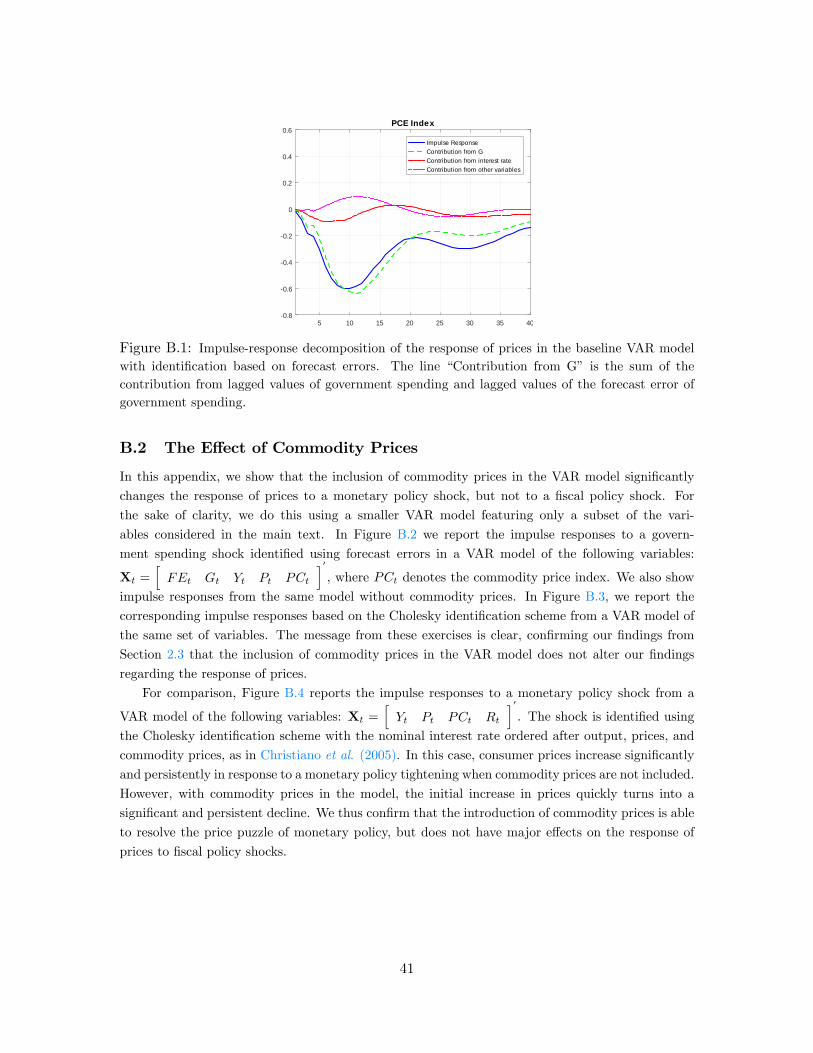
5 10 15 20 25 30 35 40­0.8

­0.6

­0.4

­0.2

0

0.2

0.4

0.6PCE Index

Impulse ResponseContribution from GContribution from interest rateContribution from other variables

Figure B.1: Impulse-response decomposition of the response of prices in the baseline VAR modelwith identification based on forecast errors. The line “Contribution from G” is the sum of thecontribution from lagged values of government spending and lagged values of the forecast error ofgovernment spending.

B.2 The Effect of Commodity Prices

In this appendix, we show that the inclusion of commodity prices in the VAR model significantly

changes the response of prices to a monetary policy shock, but not to a fiscal policy shock. For

the sake of clarity, we do this using a smaller VAR model featuring only a subset of the vari-

ables considered in the main text. In Figure B.2 we report the impulse responses to a govern-

ment spending shock identified using forecast errors in a VAR model of the following variables:

Xt =[FEt Gt Yt Pt PCt

]′, where PCt denotes the commodity price index. We also show

impulse responses from the same model without commodity prices. In Figure B.3, we report the

corresponding impulse responses based on the Cholesky identification scheme from a VAR model of

the same set of variables. The message from these exercises is clear, confirming our findings from

Section 2.3 that the inclusion of commodity prices in the VAR model does not alter our findings

regarding the response of prices.

For comparison, Figure B.4 reports the impulse responses to a monetary policy shock from a

VAR model of the following variables: Xt =[Yt Pt PCt Rt

]′. The shock is identified using

the Cholesky identification scheme with the nominal interest rate ordered after output, prices, and

commodity prices, as in Christiano et al. (2005). In this case, consumer prices increase significantly

and persistently in response to a monetary policy tightening when commodity prices are not included.

However, with commodity prices in the model, the initial increase in prices quickly turns into a

significant and persistent decline. We thus confirm that the introduction of commodity prices is able

to resolve the price puzzle of monetary policy, but does not have major effects on the response of

prices to fiscal policy shocks.

41

0 10 20 30 40­1

0

1

2Government Spending

0 10 20 30 40­0.5

0

0.5

1

1.5Output

0 10 20 30 40­1.5

­1

­0.5

0

0.5PCE index

0 10 20 30 40­3

­2

­1

0

1Commodity Prices

Figure B.2: The dynamic effects of a shock to government spending with (blue lines) andwithout (red lines) commodity prices in the VAR model. Estimates obtained using the iden-tification scheme based on forecast errors. Dashed blue and dotted red lines represent 68percent confidence intervals from the models with and without commodity prices, respec-tively.

0 10 20 30 40­0.5

0

0.5

1

1.5Government Spending

0 10 20 30 40­0.2

0

0.2

0.4Output

0 10 20 30 40­0.6

­0.4

­0.2

0

0.2PCE index

0 10 20 30 40­1

­0.5

0

0.5Commodity Prices

Figure B.3: The dynamic effects of a shock to government spending with (blue lines) andwithout (red lines) commodity prices in the VAR model. Estimates obtained using theCholesky identification scheme. Dashed blue and dotted red lines represent 68 percent con-fidence intervals from the models with and without commodity prices, respectively.

42

0 10 20 30 40­10

­5

0

5 10­3 Output

0 10 20 30 40­0.01

­0.005

0

0.005

0.01PCE index

0 10 20 30 40­0.02

­0.01

0

0.01

0.02Commodity Prices

0 10 20 30 40­0.5

0

0.5

1

1.5Interest Rate

Figure B.4: The dynamic effects of a shock to the monetary policy interest rate with (bluelines) and without (red lines) commodity prices in the VAR model. Estimates obtained usingthe Cholesky identification scheme. Dashed blue and dotted red lines represent 68 percentconfidence intervals from the models with and without commodity prices, respectively.

C Robustness Checks

This appendix contains a set of robustness checks. The first three figures report robustness checksfrom our baseline VAR model with identification based on forecast errors.32 The next three figuresshow the same set of robustness checks for the VAR model with identification based on a Choleskydecomposition. Finally, we present the results obtained when we add software expenditures to ourbaseline VAR model in Figures C.7-C.8.

32The alternative ordering used in some of the robustness checks below is the following: Xt =[FEt Gt Tt Yt Ct Pt At Rt

]′. We have experimented with other alternative orderings, in par-

ticular regarding the placement of the price index. This did not lead to any changes in our results.

43

GDP Defl.

0 5 10 15 20 25 30 35 40­0.5

0

0.5

1

1.5

Gov

.Spe

ndin

g

0 5 10 15 20 25 30 35 40­0.5

0

0.5

1

1.5

Out

put

0 5 10 15 20 25 30 35 40­0.5

0

0.5

1

1.5

Priv

ateC

ons.

0 5 10 15 20 25 30 35 40­2

0

2

4

6

8

Taxe

s

0 5 10 15 20 25 30 35 40­1

­0.5

0

0.5

Pric

eInd

ex

0 5 10 15 20 25 30 35 40­80

­40

0

40

Int.R

ate

0 5 10 15 20 25 30 35 40­0.4

0

0.4

0.8

Prod

uctiv

ity

CPI

0 5 10 15 20 25 30 35 40­0.5

0

0.5

1

1.5

0 5 10 15 20 25 30 35 40­0.5

0

0.5

1

1.5

0 5 10 15 20 25 30 35 40­0.5

0

0.5

1

1.5

0 5 10 15 20 25 30 35 40­2

0

2

4

6

8

0 5 10 15 20 25 30 35 40­1

­0.5

0

0.5

0 5 10 15 20 25 30 35 40­80

­40

0

40

0 5 10 15 20 25 30 35 40­0.4

0

0.4

0.8

PCE Core

0 5 10 15 20 25 30 35 40­0.5

0

0.5

1

1.5

0 5 10 15 20 25 30 35 40­0.5

0

0.5

1

1.5

0 5 10 15 20 25 30 35 40­0.5

0

0.5

1

1.5

0 5 10 15 20 25 30 35 40­2

0

2

4

6

8

0 5 10 15 20 25 30 35 40­1

­0.5

0

0.5

0 5 10 15 20 25 30 35 40­80

­40

0

40

0 5 10 15 20 25 30 35 40­0.4

0

0.4

0.8

Figure C.1: The dynamic effects of a shock to government spending. Robustness checks:Different price indices: GDP deflator (first column), CPI index (second column), PCE coreprice index (third column). Estimates obtained using the identification scheme based onforecast errors. The black line denotes the estimated response, while the grey areas represent68 percent confidence bands.

44

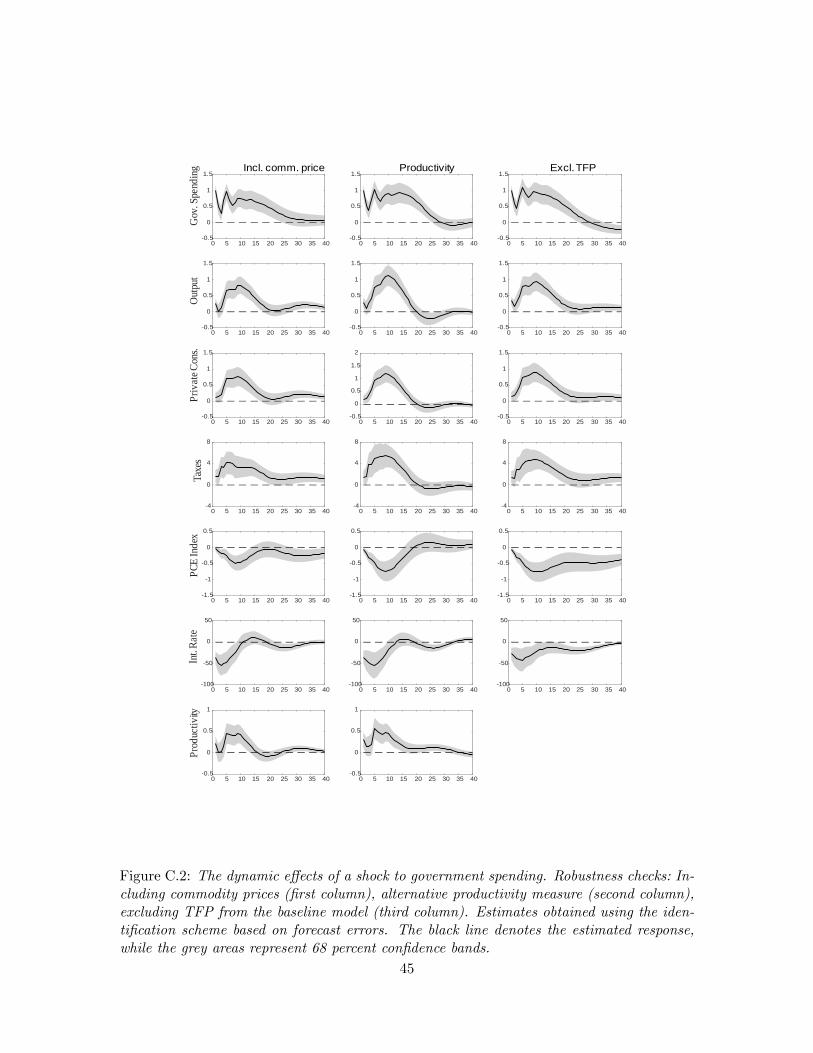
Excl. TFP

0 5 10 15 20 25 30 35 40­0.5

0

0.5

1

1.5

0 5 10 15 20 25 30 35 40­0.5

0

0.5

1

1.5

0 5 10 15 20 25 30 35 40­0.5

0

0.5

1

1.5

0 5 10 15 20 25 30 35 40­4

0

4

8

0 5 10 15 20 25 30 35 40­1.5

­1

­0.5

0

0.5

0 5 10 15 20 25 30 35 40­100

­50

0

50

Productivity

0 5 10 15 20 25 30 35 40­0.5

0

0.5

1

1.5

0 5 10 15 20 25 30 35 40­0.5

0

0.5

1

1.5

0 5 10 15 20 25 30 35 40­0.5

0

0.5

1

1.5

2

0 5 10 15 20 25 30 35 40­4

0

4

8

0 5 10 15 20 25 30 35 40­1.5

­1

­0.5

0

0.5

0 5 10 15 20 25 30 35 40­100

­50

0

50

0 5 10 15 20 25 30 35 40­0.5

0

0.5

1

Incl. comm. price

0 5 10 15 20 25 30 35 40­0.5

0

0.5

1

1.5

Gov

.Spe

ndin

g

0 5 10 15 20 25 30 35 40­0.5

0

0.5

1

1.5

Out

put

0 5 10 15 20 25 30 35 40­0.5

0

0.5

1

1.5

Priv

ateC

ons.

0 5 10 15 20 25 30 35 40­4

0

4

8

Taxe

s

0 5 10 15 20 25 30 35 40­1.5

­1

­0.5

0

0.5

PCE

Inde

x

0 5 10 15 20 25 30 35 40­100

­50

0

50

Int.R

ate

0 5 10 15 20 25 30 35 40­0.5

0

0.5

1

Prod

uctiv

ity

Figure C.2: The dynamic effects of a shock to government spending. Robustness checks: In-cluding commodity prices (first column), alternative productivity measure (second column),excluding TFP from the baseline model (third column). Estimates obtained using the iden-tification scheme based on forecast errors. The black line denotes the estimated response,while the grey areas represent 68 percent confidence bands.

45

Order

0 5 10 15 20 25 30 35 40­1

0

1

2

Gov

.Spe

ndin

g

0 5 10 15 20 25 30 35 40­8

­4

0

4

8

12

Taxe

s

0 5 10 15 20 25 30 35 40­1

­0.50

0.5

11.5

2

Out

put

0 5 10 15 20 25 30 35 40­1

­0.50

0.5

11.5

2

Priv

ateC

ons.

0 5 10 15 20 25 30 35 40­1

­0.5

0

0.5

Pric

eInd

ex

0 5 10 15 20 25 30 35 40­0.4

0

0.4

0.8

1.2

Prod

uctiv

ity

0 5 10 15 20 25 30 35 40­80

­40

0

40

80

Int.R

ate

6 lags

0 5 10 15 20 25 30 35 40­1

0

1

2

0 5 10 15 20 25 30 35 40­1

­0.50

0.5

11.5

2

0 5 10 15 20 25 30 35 40­1

­0.50

0.5

11.5

2

0 5 10 15 20 25 30 35 40­8

­4

0

4

8

12

0 5 10 15 20 25 30 35 40­1

­0.5

0

0.5

0 5 10 15 20 25 30 35 40­80

­40

0

40

80

0 5 10 15 20 25 30 35 40­0.4

0

0.4

0.8

1.2

Excl. quadr. trend

0 5 10 15 20 25 30 35 40­1

0

1

2

0 5 10 15 20 25 30 35 40­1

­0.50

0.5

11.5

2

0 5 10 15 20 25 30 35 40­1

­0.50

0.5

11.5

2

0 5 10 15 20 25 30 35 40­8

­4

0

4

8

12

0 5 10 15 20 25 30 35 40­2

­1.5

­1

­0.5

0

0.5

0 5 10 15 20 25 30 35 40­80

­40

0

40

80

0 5 10 15 20 25 30 35 40­0.4

0

0.4

0.8

1.2

Figure C.3: The dynamic effects of a shock to government spending. Robustness checks:Alternative ordering of variables (first column), model with 6 lags instead of 4 (secondcolumn), model excluding the quadratic trend (third column). Estimates obtained using theidentification scheme based on forecast errors. The black line denotes the estimated response,while the grey areas represent 68 percent confidence bands.

46

GDP Defl.

0 5 10 15 20 25 30 35 40­0.5

0

0.5

1

1.5

Gov

.Spe

ndin

g

0 5 10 15 20 25 30 35 40­0.1

0

0.1

0.2

0.3

0.4

Out

put

0 5 10 15 20 25 30 35 40­0.1

0

0.1

0.2

0.3

0.4

Priv

ateC

ons.

0 5 10 15 20 25 30 35 40­2.5

­2­1.5

­1

­0.50

0.5

Taxe

s

0 5 10 15 20 25 30 35 40­0.6

­0.4

­0.2

0

Pric

eInd

ex

0 5 10 15 20 25 30 35 40­30

­20

­10

0

10

Int.R

ate

0 5 10 15 20 25 30 35 400

0.1

0.2

0.3

Prod

uctiv

ity

CPI

0 5 10 15 20 25 30 35 40­0.5

0

0.5

1

1.5

0 5 10 15 20 25 30 35 40­0.1

0

0.1

0.2

0.3

0.4

0 5 10 15 20 25 30 35 40­0.1

0

0.1

0.2

0.3

0.4

0 5 10 15 20 25 30 35 40­2.5

­2­1.5

­1

­0.50

0.5

0 5 10 15 20 25 30 35 40­0.6

­0.4

­0.2

0

0 5 10 15 20 25 30 35 40­30

­20

­10

0

10

0 5 10 15 20 25 30 35 400

0.1

0.2

0.3

PCE Core

0 5 10 15 20 25 30 35 40­0.5

0

0.5

1

1.5

0 5 10 15 20 25 30 35 40­0.1

0

0.1

0.2

0.3

0.4

0 5 10 15 20 25 30 35 40­0.1

0

0.1

0.2

0.3

0.4

0 5 10 15 20 25 30 35 40­2.5

­2­1.5

­1

­0.50

0.5

0 5 10 15 20 25 30 35 40­0.6

­0.4

­0.2

0

0 5 10 15 20 25 30 35 40­30

­20

­10

0

10

0 5 10 15 20 25 30 35 400

0.1

0.2

0.3

Figure C.4: The dynamic effects of a shock to government spending. Robustness checks:Different price indices: GDP deflator (first column), CPI index (second column), PCE coreprice index (third column). Estimates obtained using the identification scheme based onCholesky identification scheme. The black line denotes the estimated response, while thegrey areas represent 68 percent confidence bands.

47

Excl. TFP

0 5 10 15 20 25 30 35 40­0.5

0

0.5

1

1.5

0 5 10 15 20 25 30 35 40­0.1

0

0.1

0.2

0.3

0.4

0 5 10 15 20 25 30 35 40­0.1

0

0.1

0.2

0.3

0.4

0 5 10 15 20 25 30 35 40­3

­2

­1

0

1

0 5 10 15 20 25 30 35 40­0.8

­0.6

­0.4

­0.2

0

0 5 10 15 20 25 30 35 40­40

­30

­20

­10

0

10

Productivity

0 5 10 15 20 25 30 35 40­0.5

0

0.5

1

1.5

0 5 10 15 20 25 30 35 40­0.1

0

0.1

0.2

0.3

0.4

0 5 10 15 20 25 30 35 40­0.1

0

0.1

0.2

0.3

0.4

0 5 10 15 20 25 30 35 40­3

­2

­1

0

1

0 5 10 15 20 25 30 35 40­0.8

­0.6

­0.4

­0.2

0

0 5 10 15 20 25 30 35 40­40

­30

­20

­10

0

10

0 5 10 15 20 25 30 35 400

0.1

0.2

0.3

0.4

Incl. comm. price

0 5 10 15 20 25 30 35 40­0.5

0

0.5

1

1.5

Gov

.Spe

ndin

g

0 5 10 15 20 25 30 35 40­0.1

0

0.1

0.2

0.3

0.4

Out

put

0 5 10 15 20 25 30 35 40­0.1

0

0.1

0.2

0.3

0.4

Priv

ateC

ons.

0 5 10 15 20 25 30 35 40­3

­2

­1

0

1

Taxe

s

0 5 10 15 20 25 30 35 40­0.8

­0.6

­0.4

­0.2

0

PCE

Inde

x

0 5 10 15 20 25 30 35 40­40

­30

­20

­10

0

10

Int.R

ate

0 5 10 15 20 25 30 35 400

0.1

0.2

0.3

0.4

Prod

uctiv

ity

Figure C.5: The dynamic effects of a shock to government spending. Robustness checks:Including commodity prices (first column), alternative productivity measure (second col-umn), excluding TFP from the baseline model (third column). Estimates obtained using theidentification scheme based on Cholesky identification scheme. The black line denotes theestimated response, while the grey areas represent 68 percent confidence bands.

48

Order

0 5 10 15 20 25 30 35 40­0.5

0

0.5

1

1.5

Gov

.Spe

ndin

g

0 5 10 15 20 25 30 35 40­3

­2

­1

0

1

2

Taxe

s

0 5 10 15 20 25 30 35 40­0.2

0

0.2

0.4

0.6

Out

put

0 5 10 15 20 25 30 35 40­0.2

0

0.2

0.4

0.6

Priv

ateC

ons.

0 5 10 15 20 25 30 35 40­0.6

­0.3

0

Pric

eInd

ex

0 5 10 15 20 25 30 35 40­0.2

0

0.2

0.4

Prod

uctiv

ity

0 5 10 15 20 25 30 35 40­40

­30

­20

­10

0

10

Int.R

ate

6 lags

0 5 10 15 20 25 30 35 40­0.5

0

0.5

1

1.5

0 5 10 15 20 25 30 35 40­0.2

0

0.2

0.4

0.6

0 5 10 15 20 25 30 35 40­0.2

0

0.2

0.4

0.6

0 5 10 15 20 25 30 35 40­3

­2

­1

0

1

2

0 5 10 15 20 25 30 35 40­0.6

­0.3

0

0 5 10 15 20 25 30 35 40­40

­30

­20

­10

0

10

0 5 10 15 20 25 30 35 40­0.2

0

0.2

0.4

Excl. quadr. trend

0 5 10 15 20 25 30 35 40­0.5

0

0.5

1

1.5

0 5 10 15 20 25 30 35 40­0.4

­0.2

0

0.2

0.4

0 5 10 15 20 25 30 35 40­0.4

­0.2

0

0.2

0.4

0 5 10 15 20 25 30 35 40­3

­2

­1

0

1

2

0 5 10 15 20 25 30 35 40­1.5

­1

­0.5

0

0 5 10 15 20 25 30 35 40­40

­30

­20

­10

0

10

0 5 10 15 20 25 30 35 40­0.2

0

0.2

0.4

Figure C.6: The dynamic effects of a shock to government spending. Robustness checks:Alternative ordering of variables (first column), model with 6 lags instead of 4 (secondcolumn), model excluding the quadratic trend (third column). Estimates obtained using theCholesky identification scheme. The black line denotes the estimated response, while thegrey areas represent 68 percent confidence bands.

49

Government Spending

0 10 20 30 40­0.5

0

0.5

1

1.5Output

0 10 20 30 40­0.5

0

0.5

1

1.5

Private Cons.

0 10 20 30 40­0.5

0

0.5

1

1.5Taxes

0 10 20 30 40­5

0

5

10

PCE index

0 10 20 30 40­1

­0.5

0

0.5Int. Rate

0 10 20 30 40­100

­50

0

50

TFP

0 10 20 30 40­0.5

0

0.5

1Software Expenditures

0 10 20 30 40­2

0

2

4

Figure C.7: The dynamic effects of a shock to government spending. Model augmented withsoftware expenditure. Estimates obtained using the identification scheme based on forecasterrors. The black line denotes the estimated response, while the grey areas represent 68percent confidence bands.

50

Government Spending

0 10 20 30 40­0.5

0

0.5

1

1.5Output

0 10 20 30 40­0.2

0

0.2

0.4

Private Cons.

0 10 20 30 40­0.1

0

0.1

0.2Taxes

0 10 20 30 40­2

­1

0

1

PCE index

0 10 20 30 40­0.4

­0.2

0

0.2Int. Rate

0 10 20 30 40­20

­10

0

10

TFP

0 10 20 30 40­0.1

0

0.1

0.2

0.3Software Expenditures

0 10 20 30 40­1

0

1

2

Figure C.8: The dynamic effects of a shock to government spending. Model augmentedwith software expenditure. Estimates obtained using the Cholesky identification scheme.The black line denotes the estimated response, while the grey areas represent 68 percentconfidence bands.

51

D The Model

This appendix presents the details of our model of variable technology utilization. We impose thefunctional form of z (ut) proposed in (19) throughout the appendix.

D.1 The Steady State

As usual, the steady-state interest rate is pinned down by the inverse of the household’s discountfactor; R = 1/β. From the optimal price setting of intermediate goods firms (10), we obtain mc =ε−1ε . From the goods market clearing condition (16), we get:

C

Y= 1− g

Y,

where gY is determined exogenously. Steady-state production is pinned down from (5):

Y = uAN1−α,

where A is exogenous, u is fixed at 1 in steady state, and N is fixed at N = 0.25. Combining laborsupply (2) and labor demand (8), and using the production function, we can find the value of ψ thatensures this:

ψNϕ = C−σt (1− α)mcY

N⇔

ψNϕ = C−σ (1− α)mcuAN−α ⇔

ψ =(1− α)mcuA

Nϕ+αCσ.

Finally, to ensure that the utilization rate equals 1 in steady state, we rewrite (9) to get:

z′ (1) = mcY

u⇔

χ1 = mcY

u,

which pins down the required value of χ1. This completes the characterization of the steady state.

D.2 Log-linearized Model

Before simulating the model, we log-linearize it around the non-stochastic steady state. Letting xtdenote the log deviation of a generic variable xt from its steady-state value x, we obtain the followingset of log-linearized equilibrium conditions:

ϕNt = −σCt + wt, (D.1)

− σCt = Et(−σCt+1 + Rt − πt+1

), (D.2)

Yt = ut + At + (1− α) Nt, (D.3)

C

YCt = Yt −mcut −

g

Ygt, (D.4)

χ2χ1ut = mct + Yt − ut, (D.5)

52

mct = wt − ut − At + αNt, (D.6)

πt = βEtπt+1 +ε− 1

γmct, (D.7)

Rt = φππt + φyYt, (D.8)

gt = ρGgt−1 + εGt , (D.9)

At = ρAAt−1 + εAt . (D.10)

We thus have a system of 10 equations in 10 variables: Yt, Ct, gt, πt, mct, ut, wt, At, Nt, Rt.

D.3 Analytical Solution

As described in the main text, we derive the analytical solution to the model under the followingsimplifying assumptions: No technology shocks (At = 0), constant returns to scale in production(α = 0), log utility in consumption (σ = 1), unitary (inverse) Frisch elasticity of labor supply(ϕ = 1), and no monetary policy reaction to the output gap (φy = 0). Under these assumptions,it is straightforward to verify that (D.2) and (D.8) can be combined to obtain the Euler equationpresented in Section 4:

− Ct = Et(−Ct+1 + φππt − πt+1

). (D.11)

To arrive at the New Keynesian Phillips Curve studied in Section 4, we begin by combining (D.1)and (D.3) to obtain:

Yt = ut − Ct + wt.

This expression can be inserted twice, into (D.4) and (D.5), to obtain:

C

YCt = ut − Ct + wt −mcut −

g

Ygt ⇔

wt =

(1 +

C

Y

)Ct − (1−mc) ut +

g

Ygt, (D.12)

and

χ2χ1ut = mct + ut − Ct + wt − ut ⇔

χ2χ1ut = wt − ut − Ct + wt ⇔

2wt =

(χ2χ1

+ 1

)ut + Ct,

where the second-to-last line uses (D.6). We can combine these two expressions:

(1 +

C

Y

)Ct − (1−mc) ut +

g

Ygt =

(χ2χ1

+ 1)ut + Ct

2⇔

ut =

(1 + 2C

Y

)χ2χ1

+ 1 + 2 (1−mc) Ct +2gY

χ2χ1

+ 1 + 2 (1−mc) gt. (D.13)

53

We are now ready to insert into the original New Keynesian Phillips Curve (D.7), using first (D.6):

πt = βEtπt+1 +ε− 1

γmct ⇔

πt = βEtπt+1 +ε− 1

γ(wt − ut) ,

and then inserting from (D.12):

πt = βEtπt+1 +ε− 1

γ

((1 +

C

Y

)Ct − (2−mc) ut +

g

Ygt

),

where we can insert from (D.13) to get:

πt = βEtπt+1 +ε− 1

γ

((1 +

C

Y

)Ct +

g

Ygt

)−ε− 1

γ(2−mc)

[ (1 + 2C

Y

)χ2χ1

+ 1 + 2 (1−mc) Ct +2gY

χ2χ1

+ 1 + 2 (1−mc) gt

],

which can be rewritten as:

πt = βEtπt+1 +ε− 1

γ

χ2χ1

+ 1 +(χ2χ1− 1)CY −mc

χ2χ1

+ 3− 2mcCt +

gY

(χ2χ1− 1)

χ2χ1

+ 3− 2mcgt

⇔πt = βEtπt+1 + aCt − bgt, (D.14)

after defining

a =ε− 1

γ

χ2χ1

+ 1 +(χ2χ1− 1)CY −mc

χ2χ1

+ 3− 2mc, (D.15)

b =ε− 1

γ

gY

(1− χ2

χ1

)χ2χ1

+ 3− 2mc. (D.16)

Equations (D.11) and (D.14) can be combined with (D.9) to obtain 3 equations in πt, Ct, and gt. Wecan solve this system analytically using the method of undetermined coeffi cients. For expositionalsimplicity, we assume that the shock to government spending has no persistence (ρG = 0). Weconjecture that the solutions for πt and Ct take the form:

Ct = Ψgt,

πt = Φgt,

where the coeffi cients Ψ and Φ are yet to be determined. Inserting these conjectured solutions into(D.11) and (D.14), we obtain:

−Ct = Et(−Ct+1 + φππt − πt+1

)⇔

−Ψgt = Et (−Ψgt+1 + φπΦgt − Φgt+1)⇔Ψ = −φπΦ,

54

where we have used that Etgt+1 = 0 when shocks have no persistence. Further, we get:

πt = βEtπt+1 +ε− 1

γ

χ2χ1

+ 1 +(χ2χ1− 1)CY −mc

χ2χ1

+ 3− 2mcCt +

gY

(χ2χ1− 1)

χ2χ1

+ 3− 2mcgt

⇔Φgt = βEtΦgt+1 +

ε− 1

γ

χ2χ1

+ 1 +(χ2χ1− 1)CY −mc

χ2χ1

+ 3− 2mcΨgt +

gY

(χ2χ1− 1)

χ2χ1

+ 3− 2mcgt

⇔Φ =

ε− 1

γ

χ2χ1

+ 1 +(χ2χ1− 1)CY −mc

χ2χ1

+ 3− 2mcΨ +

gY

(χ2χ1− 1)

χ2χ1

+ 3− 2mc

.

Combining these two expressions yields:

Φ =ε− 1

γ

− χ2χ1

+ 1 +(χ2χ1− 1)CY −mc

χ2χ1

+ 3− 2mcφπΦ +

gY

(χ2χ1− 1)

χ2χ1

+ 3− 2mc

⇔

Φ

1 +ε− 1

γφπ

χ2χ1

+ 1 +(χ2χ1− 1)CY −mc

χ2χ1

+ 3− 2mc

=ε− 1

γ

gY

(χ2χ1− 1)

χ2χ1

+ 3− 2mc⇔

Φ

ε−1γ φπ

[χ2χ1

+ 1 +(χ2χ1− 1)CY −mc

]+ χ2

χ1+ 3− 2mc

χ2χ1

+ 3− 2mc=

ε− 1

γ

gY

(χ2χ1− 1)

χ2χ1

+ 3− 2mc⇔

Φ =

ε−1γ

gY

(χ2χ1− 1)

ε−1γ φπ

[χ2χ1

+ 1 +(χ2χ1− 1)CY −mc

]+ χ2

χ1+ 3− 2mc

,

and then:

Ψ = −φπΦ⇔

Ψ = −φπ

ε−1γ

gY

(χ2χ1− 1)

ε−1γ φπ

[χ2χ1

+ 1 +(χ2χ1− 1)CY −mc

]+ χ2

χ1+ 3− 2mc

,

so that the solution is:

Ct = −φπ

ε−1γ

gY

(χ2χ1− 1)

ε−1γ φπ

[χ2χ1

+ 1 +(χ2χ1− 1)CY −mc

]+ χ2

χ1+ 3− 2mc

gt, (D.17)

πt =

ε−1γ

gY

(χ2χ1− 1)

ε−1γ φπ

[χ2χ1

+ 1 +(χ2χ1− 1)CY −mc

]+ χ2

χ1+ 3− 2mc

gt. (D.18)

This confirms the form of our conjectured solution, and provides us with closed-form expressions ofhow consumption and inflation react to a government spending shock on impact. To establish the

55

sign of these coeffi cients, we first note that the denominator is positive whenever:

ε− 1

γφπ

[χ2χ1

+ 1 +

(χ2χ1− 1

)C

Y−mc

]+χ2χ1

+ 3− 2mc > 0⇔

χ2χ1

[1 +

ε− 1

γφπ

(1 +

C

Y

)]> mc

(2 + φπ

ε− 1

γ

)− 3− ε− 1

γφπ

(1− C

Y

)⇔

χ2 > χ1

mc(

2 + φπε−1γ

)− 3− ε−1

γ φπ(1− C

Y

)1 + ε−1

γ φπ(1 + C

Y

) . (D.19)

This is a lower bound on χ2. We show below that this condition is always satisfied when the modelhas a unique and determinate solution. We therefore obtain a decline in inflation and an increase inconsumption if and only if the numerators in both expressions are negative:

φπε− 1

γ

g

Y

(χ2χ1− 1

)< 0⇔(

χ2χ1− 1

)< 0⇔

χ2 < χ1. (D.20)

This is the condition stated in Proposition 2 in the main text. However, to complete the proof, thenext subsection derives the conditions for the model to have a unique and stable equilibrium.

D.4 Equilibrium Determinacy and Uniqueness

The system consisting of (D.11) and (D.14) has two non-predetermined variables. This implies thata necessary and suffi cient condition for the model to have a unique and determinate equilibrium isthat both eigenvalues of the characteristic polynomial should be inside the unit circle. To write upthe characteristic polynomial, we first restate the system on matrix form. After some algebra, wearrive at the following expression:[

Ctπt

]= Ω

[Υ (1− βφπ) ΥΓ Γ + βΥ

] [EtCt+1Etπt+1

]+ ΩΞ

[−φπ

1

]gt ⇔[

Ctπt

]= A0

[EtCt+1Etπt+1

]+B0gt, A0 ≡ Ω

[Υ (1− βφπ) ΥΓ Γ + βΥ

], B0 ≡ ΩΞ

[φπ1

],

where we have defined:

Ω ≡ 1χ2χ1

+ 3− 2mc+ φπ(ε−1)γ

[χ2χ1

+ 1 +(χ2χ1− 1)CY −mc

] ,Γ ≡ ε− 1

γ

[χ2χ1

+ 1 +

(χ2χ1− 1

)C

Y−mc

],

Ξ ≡ ε− 1

γ

(χ2χ1− 1

)g

Y,

Υ ≡(χ2χ1

+ 3− 2mc

).

56

The characteristic polynomial is then:

|A0 − λI| = 0⇔∣∣∣∣Ω [ Υ (1− βφπ) ΥΓ Γ + βΥ

]− λ

[1 00 1

]∣∣∣∣ = 0⇔

0 =

∣∣∣∣∣∣∣∣

(χ2χ1+3−2mc

)χ2χ1+3−2mc+φπ(ε−1)

γ

[χ2χ1+1+

(χ2χ1−1)CY −mc

] − λ (1−βφπ)(χ2χ1+3−2mc

)χ2χ1+3−2mc+φπ(ε−1)

γ

[χ2χ1+1+

(χ2χ1−1)CY −mc

]ε−1γ

[χ2χ1+1+

(χ2χ1−1)CY −mc

]χ2χ1+3−2mc+φπ(ε−1)

γ

[χ2χ1+1+

(χ2χ1−1)CY −mc

] ε−1γ

[χ2χ1+1+

(χ2χ1−1)CY −mc

]+β(χ2χ1+3−2mc

)χ2χ1+3−2mc+φπ(ε−1)

γ

[χ2χ1+1+

(χ2χ1−1)CY −mc

] − λ

∣∣∣∣∣∣∣∣ .

After some tedious algebra, we are able to restate the implied second-order polynomial as:

0 = λ2 + a1λ+ a0,

where we have defined:

a1 ≡ −(1 + β)

(χ2χ1

+ 3− 2mc)

+ ε−1γ

[χ2χ1

+ 1 +(χ2χ1− 1)CY −mc

]χ2χ1

+ 3− 2mc+ φπ(ε−1)γ

[χ2χ1

+ 1 +(χ2χ1− 1)CY −mc

] ,

a0 ≡β(χ2χ1

+ 3− 2mc)

χ2χ1

+ 3− 2mc+ φπ(ε−1)γ

[χ2χ1

+ 1 +(χ2χ1− 1)CY −mc

] .We know from, e.g., LaSalle (1986) that both eigenvalues are inside the unit circle if and only ifboth of the following conditions are satisfied:

|a0| < 1, (D.21)

|a1| < 1 + a0. (D.22)

We can check these in turn. The first condition yields:∣∣∣∣∣∣β(χ2χ1

+ 3− 2mc)

(χ2χ1

+ 3− 2mc)

+ φπ(ε−1)γ

[χ2χ1

+ 1 +(χ2χ1− 1)CY −mc

]∣∣∣∣∣∣ < 1.

Since β < 1 and the bracket in the numerator is always positive, the denominator will be larger thanthe numerator (and thus, the inequality satisfied) as long as the second term in the denominator isnon-negative:

φπ (ε− 1)

γ

[χ2χ1

+ 1 +

(χ2χ1− 1

)C

Y−mc

]> 0⇔

χ2χ1

+ 1 +

(χ2χ1− 1

)(1− g

Y

)−mc > 0⇔

χ2χ1

(1 +

(1− g

Y

))> mc+

(1− g

Y

)− 1⇔

χ2χ1

>mc− g

Y

2− gY

. (D.23)

57

This is the condition stated in Proposition 1 in the main text, providing another lower bound on χ2.We can verify that this is the relevant, binding lower bound on χ2 by showing that this expressionis strictly larger than the one implied by (D.19):

χ1mc− g

Y

2− gY

> χ1

mc(

2 + φπε−1γ

)− 3− ε−1

γ φπ(1− C

Y

)1 + ε−1

γ φπ(1 + C

Y

) ⇔

(mc− g

Y

)[1 +

ε− 1

γφπ

(1 +

C

Y

)]>

(2− g

Y

)[mc

(2 + φπ

ε− 1

γ

)− 3− ε− 1

γφπ

(1− C

Y

)]⇔

6 > 2g

Y(2−mc) + 3mc,

where the last step follows from some simple but tedious algebra. The right-hand side is maximizedwhen g

Y reaches its upper bound of 1 and mc reaches its upper bound of 1 (when ε → ∞). In thiscase, the right-hand side approaches 5. We can thus conclude that this condition is always satisfied,so that the binding lower bound on χ2 is given from (D.23).

Consider now the second necessary and suffi cient condition for a unique and determinate equi-librium, (D.22), which yields:

|a1| < 1 + a0 ⇔

∣∣∣∣∣∣−(1 + β)

(χ2χ1

+ 3− 2mc)

+ ε−1γ

[χ2χ1

+ 1 +(χ2χ1− 1)CY −mc

]χ2χ1

+ 3− 2mc+ φπ(ε−1)γ

[χ2χ1

+ 1 +(χ2χ1− 1)CY −mc

]∣∣∣∣∣∣ <

1 +β(χ2χ1

+ 3− 2mc)

χ2χ1

+ 3− 2mc+ φπ(ε−1)γ

[χ2χ1

+ 1 +(χ2χ1− 1)CY −mc

] ⇔

∣∣∣∣∣∣−(1 + β)

(χ2χ1

+ 3− 2mc)

+ ε−1γ

[χ2χ1

+ 1 +(χ2χ1− 1)CY −mc

](χ2χ1

+ 3− 2mc)

+ φπ(ε−1)γ

[χ2χ1

+ 1 +(χ2χ1− 1)CY −mc

]∣∣∣∣∣∣ <

β(χ2χ1

+ 3− 2mc)

+ χ2χ1

+ 3− 2mc+ φπ(ε−1)γ

[χ2χ1

+ 1 +(χ2χ1− 1)CY −mc

](χ2χ1

+ 3− 2mc)

+ φπ(ε−1)γ

[χ2χ1

+ 1 +(χ2χ1− 1)CY −mc

] .

We saw above that the last term in the denominator is positive, and we have established that alsothe first term is positive, so we can cancel out the denominators:∣∣∣∣− [(1 + β)

(χ2χ1

+ 3− 2mc

)+ε− 1

γ

(χ2χ1

+ 1 +

(χ2χ1− 1

)C

Y−mc

)]∣∣∣∣ <(1 + β)

(χ2χ1

+ 3− 2mc

)+φπ (ε− 1)

γ

[χ2χ1

+ 1 +

(χ2χ1− 1

)C

Y−mc

].

Using the same insights, we conclude that all terms on the left-hand side must be positive, so takingabsolute values yields:

(1 + β)

(χ2χ1

+ 3− 2mc

)+ε− 1

γ

(χ2χ1

+ 1 +

(χ2χ1− 1

)C

Y−mc

)<

(1 + β)

(χ2χ1

+ 3− 2mc

)+φπ (ε− 1)

γ

[χ2χ1

+ 1 +

(χ2χ1− 1

)C

Y−mc

]⇔

58

ε− 1

γ

[χ2χ1

+ 1 +

(χ2χ1− 1

)C

Y−mc

]<φπ (ε− 1)

γ

[χ2χ1

+ 1 +

(χ2χ1− 1

)C

Y−mc

]⇔

φπ > 1, (D.24)

which is just the well-known Taylor-principle (in the absence of a monetary policy reaction to output,as assumed above). This condition is satisfied by assumption, as we have assumed φπ > 1 alreadyin the main text.

To sum up, we have established that the model has a unique and determinate solution if and onlyif conditions (D.23) and (D.24) are satisfied, and that when this is the case, the solution featuresan increase in consumption and a decline in inflation if and only if condition (D.20) holds. Thiscompletes the proof of Propositions 1 and 2 in the main text

As a final note, recall our graphical representation of equations (D.11) and (D.14) in Section4. Given the definition of the parameters a and b in (D.15) and (D.16), it is easy to verify thatthe condition for the parameter a to be positive, and thus for the rewritten New Keynesian PhillipsCurve (D.14) to be upward-sloping, is identical to the condition in (D.23). Likewise, it can be easilyverified that the parameter b is positive, so that a government spending shock shifts this curve down,if and only if the condition given by (D.20) is satisfied.

D.5 Detour: The Basic New Keynesian Model

In this subsection, we derive the solution to a model version without variable technology utilization.Incidentally, in this case the model collapses to the basic New Keynesian model, as presented, e.g., inGalí (2015), augmented with government spending. For comparison, we make the same assumptionsas in the simplified version of our baseline model: No technology shocks (At = 0), constant returnsto scale in production (α = 0), log utility in consumption (σ = 1), unitary (inverse) Frisch elasticityof labor supply (ϕ = 1), no monetary policy reaction to the output gap (φy = 0), and no persistencein fiscal policy shocks (ρG = 0). Under these assumptions, the basic New Keynesian model is givenby the following set of equations:

Nt = −Ct + wt,

−Ct = Et(−Ct+1 + Rt − πt+1

),

Yt = Nt,

C

YCt = Yt −

g

Ygt,

mct = wt,

πt = βEtπt+1 +ε− 1

γmct,

Rt = φππt,

plus an exogenous process for gt. We can combine these equations to obtain:33

πt = βEtπt+1 +ε− 1

γ

(Ct

(1 +

C

Y

)+g

Ygt

),

−Ct = Et(−Ct+1 + φππt − πt+1

).

33Having carefully described the analytical solution to our baseline model above, we do not present anyintermediate steps in this subsection, but simply state the results.

59

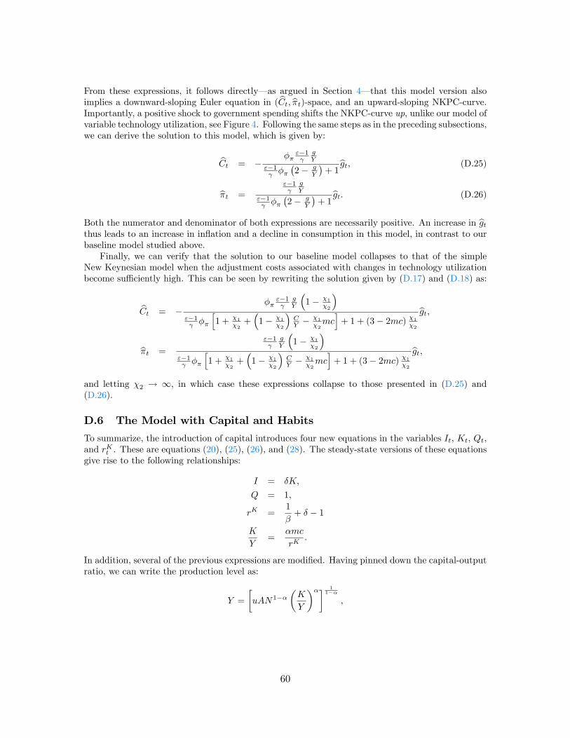
From these expressions, it follows directly– as argued in Section 4– that this model version alsoimplies a downward-sloping Euler equation in (Ct, πt)-space, and an upward-sloping NKPC-curve.Importantly, a positive shock to government spending shifts the NKPC-curve up, unlike our model ofvariable technology utilization, see Figure 4. Following the same steps as in the preceding subsections,we can derive the solution to this model, which is given by:

Ct = −φπ

ε−1γ

gY

ε−1γ φπ

(2− g

Y

)+ 1

gt, (D.25)

πt =

ε−1γ

gY

ε−1γ φπ

(2− g

Y

)+ 1

gt. (D.26)

Both the numerator and denominator of both expressions are necessarily positive. An increase in gtthus leads to an increase in inflation and a decline in consumption in this model, in contrast to ourbaseline model studied above.

Finally, we can verify that the solution to our baseline model collapses to that of the simpleNew Keynesian model when the adjustment costs associated with changes in technology utilizationbecome suffi ciently high. This can be seen by rewriting the solution given by (D.17) and (D.18) as:

Ct = −φπ

ε−1γ

gY

(1− χ1

χ2

)ε−1γ φπ

[1 + χ1

χ2+(

1− χ1χ2

)CY −

χ1χ2mc]

+ 1 + (3− 2mc) χ1χ2

gt,

πt =

ε−1γ

gY

(1− χ1

χ2

)ε−1γ φπ

[1 + χ1

χ2+(

1− χ1χ2

)CY −

χ1χ2mc]

+ 1 + (3− 2mc) χ1χ2

gt,

and letting χ2 → ∞, in which case these expressions collapse to those presented in (D.25) and(D.26).

D.6 The Model with Capital and Habits

To summarize, the introduction of capital introduces four new equations in the variables It, Kt, Qt,and rKt . These are equations (20), (25), (26), and (28). The steady-state versions of these equationsgive rise to the following relationships:

I = δK,

Q = 1,

rK =1

β+ δ − 1

K

Y=

αmc

rK.

In addition, several of the previous expressions are modified. Having pinned down the capital-outputratio, we can write the production level as:

Y =

[uAN1−α

(K

Y

)α] 11−α

,

60

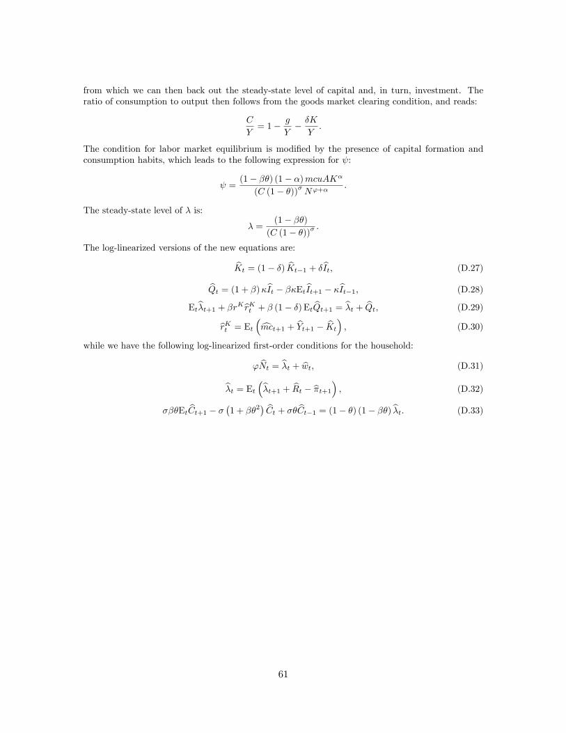
from which we can then back out the steady-state level of capital and, in turn, investment. Theratio of consumption to output then follows from the goods market clearing condition, and reads:

C

Y= 1− g

Y− δK

Y.

The condition for labor market equilibrium is modified by the presence of capital formation andconsumption habits, which leads to the following expression for ψ:

ψ =(1− βθ) (1− α)mcuAKα

(C (1− θ))σ Nϕ+α.

The steady-state level of λ is:

λ =(1− βθ)

(C (1− θ))σ .

The log-linearized versions of the new equations are:

Kt = (1− δ) Kt−1 + δIt, (D.27)

Qt = (1 + β)κIt − βκEtIt+1 − κIt−1, (D.28)

Etλt+1 + βrK rKt + β (1− δ)EtQt+1 = λt + Qt, (D.29)

rKt = Et(mct+1 + Yt+1 − Kt

), (D.30)

while we have the following log-linearized first-order conditions for the household:

ϕNt = λt + wt, (D.31)

λt = Et(λt+1 + Rt − πt+1

), (D.32)

σβθEtCt+1 − σ(1 + βθ2

)Ct + σθCt−1 = (1− θ) (1− βθ) λt. (D.33)

61