Embed Size (px)
Citation preview

Department of Economics and Finance
Working Paper No. 12-24
http://www.brunel.ac.uk/economics
Econ
omic
s an
d Fi
nanc
e W
orki
ng P
aper
Ser
ies
Weonho Yang, Jan Fidrmuc and Sugata Ghosh
Government Spending Shocks and the Multiplier: New Evidence from the U.S. Based on Natural Disasters
November 2012

1
Government Spending Shocks and the Multiplier: New Evidence from the U.S. Based on Natural Disasters
Weonho Yang, Jan Fidrmuc* and Sugata Ghosh
Department of Economics and Finance, Brunel University
November 2012
Abstract
The literature on estimating macroeconomic effects of fiscal policy requires suitable instruments to identify exogenous and unanticipated spending shocks. So far, the instrument of choice has been military build-ups. This instrument, however, largely limits the analysis to the US as few other countries have been involved in mainly extraterritorial conflicts. Moreover, the expenditure associated with military build-ups affects primarily the defense sector so that the resulting multiplier does not necessarily approximate the effects of changes to general government spending. We propose an alternative instrument: government relief expenditure in the wake of natural disasters which is more similar in its scope to general government spending. We construct a rich data set of natural disasters and the corresponding government responses at the US state level. We apply this methodology both at the state as well as national levels and show that natural disasters serve as a powerful instrument for identifying government spending shocks. Furthermore, we show that the multiplier pertaining to non-defense government spending is higher than the defense-spending multiplier estimated in the literature using military build-ups. JEL numbers: E22, E62, H30, H50, H72 Keywords: fiscal shocks, narrative approach, fiscal multiplier, natural disaster.
* Corresponding Author. Department of Economics and Finance and Centre for Economic Development and Institutions (CEDI), Brunel University; Institute of Economic Studies, Charles University; and CESifo Munich. Contact information: Department of Economics and Finance, Brunel University, Uxbridge, UB8 3PH, United Kingdom. Email: [email protected] or [email protected]. Phone: +44-1895-266-528, Web: http://www.fidrmuc.net/.
2
1. Introduction
Recently, in response to the financial crisis and its impact on the economy, many governments have increased their spending in order to stimulate economic growth, while other governments, stricken by fiscal and debt crises, were forced to cut theirs sharply. As a result, the interest in the short-run effects of government spending has been revived again. From an economic policy perspective, it is of crucial importance to know whether fiscal policy can be used as an effective tool to dampen economic fluctuations and foster growth. However, for all its importance, the effectiveness of fiscal policy still remains a controversial issue, with neoclassical and (new) Keynesian theories making dramatically different predictions in this respect.
Although most studies agree that fiscal policy stimulates output in the short-run, there is considerable disagreement regarding the size and the transmission of its effect on economic activities. There are two strands of the empirical literature on macroeconomic effects of government spending shocks. The first one relies on structural VAR models to analyze national or international data. In order to identify the government spending shocks, it requires certain assumptions such as the use of time lags and additional information such as various elasticities (Blanchard and Perotti 2002, Perotti 2005 and Giordano et al. 2007). While it has the advantage of easy implementation and application, the results are highly sensitive to these assumptions. Moreover, as Ramey (2011a) points out, the fiscal shocks identified with this method could be subject to an ‘anticipation effect’: the shocks identified by the model are expected by the private sector. Because of this criticism, the second, so called ‘narrative’, approach seeks to identify shocks to government spending by using events associated with unexpected changes in government expenditure. In particular, military build-ups (sometimes combined with contemporaneous professional forecasts of government spending) were suggested as sources of such exogenous variation in government spending (Ramey and Shapiro 1998, Burnside et al. 2004, Ramey 2011a, and Barro and Redlick 2011). It is argued that unlike the general government expenditure, wars and international tensions that lead to military build-ups are both sufficiently difficult to predict and independent of GDP.
While most of the initial literature was concerned with time-series studies, some recent analyses use panel or cross-section data to estimate the effects of fiscal policy. Ilzetzki et al. (2011) use a novel quarterly dataset of government spending in 44 countries with the structural VAR approach. They show that the impact of government spending shocks depends on the key characteristics of the country such as the level of development, exchange rate regime, openness to trade, and public indebtedness. Nakamura and Steinsson (2011), in turn, use military spending data across U.S. regions to estimate the effects of government spending in a monetary union in a narrative approach.
While the narrative approach can take better account of the anticipation effect, it has some important limitations. First, the identification strategy relies on relatively infrequent events. The US is in a rather unique position in that it was involved in several military conflicts (hot or cold) that did not unfold on its territory. Therefore, it can be argued that these conflicts gave rise to demand shocks associated with increased government spending without affecting also the supply much. That can be said about few other countries: either they were not involved in military conflicts or these took place (at least in part) on their own territory. Second, the composition of military spending differs considerably from general government spending. Therefore, estimating the macroeconomic effect of military build-ups may have limited applicability to other categories of government spending.
The effect of government spending on the economy is often summarized by a multiplier: a change of output caused by a one unit increase in government spending. As Barro and

3
Redlick (2011) indicate, the multiplier based on military build-ups is close only to the defense spending multiplier. To assess the effect of more typical fiscal stimulus packages, we are interested in the multiplier for nondefense spending such as infrastructure, health, and education and others. However, a big hurdle in obtaining estimates of nondefense multiplier is that it is hard to find a satisfactory instrument for nondefense spending because most of the variation in nondefense spending tends to be endogenous with respect to the state of economy.
Our paper contributes to the small but growing literature seeking to identify such new instruments. Serrato and Wingender (2010) use changes in allocations of federal spending to states caused by population changes identified by means of the Census every 10 years. Their estimates imply that government spending has a local income multiplier of 1.88. Shoag (2010), in turn, collects a new dataset on the returns of state pension plans which can be predictor of subsequent state government spending. He shows that state government spending has a large positive effect on in-state income with a multiplier of 2.11. Fishback and Kachanovskaya (2010) use political competiveness across states to estimate the effects of New Deal spending and find a multiplier of 1.7. Given that multipliers obtained with military build-ups tend to be lower, ranging from 0.6 to 1.2 (Ramey, 2011a; Barro and Redlick, 2011), it appears that the defense and non-defense multipliers are indeed different from each other.
In this paper, we argue that natural disasters constitute another suitable instrument to identify exogenous variation in government spending: they are relatively frequent and unexpected. Importantly, governments respond to natural disasters by spending on relief and repair as well as on precautions against future calamities.1 Natural disasters in this way cause government spending shocks, and those shocks are unexpected and sudden, making them exogenous with respect to the state of the economy.
There is already a vast literature on the short and long-run impacts of natural disaster on macroeconomics. Recently, Cavallo and Noy (2009) surveyed this literature comprehensively. According to them, the consensus is emerging that natural disasters have a negative impact on short-term economic growth. Raddatz (2007) analyzes the effects of external shocks including natural disasters on output fluctuations in low-income countries. He concludes that natural disasters cause a significant decline in output. Noy (2009) analyzes the determinants of adverse effects of natural disaster on output in the short-run and shows that countries with a higher literacy rate, better institutions, higher per capita income, higher degree of openness to trade, higher levels of government spending, more foreign exchange reserves, and higher levels of domestic credit, but with less open capital accounts are able to withstand the initial shock better and avoid spillovers into the wider economy. Raddatz (2009) shows that smaller and poorer countries are more vulnerable, especially to climatic disasters, and that the level of external debt has no relation to the output impact of any type of disaster. Loayza et al. (2009) find that while small disasters may have a positive effect due to the reconstruction efforts, large disaster have severe negative impact on the economy immediately. Skidmore and Toya (2002) and Crespo et al. (2008), in contrast, examine the long-run impact of natural disasters on growth. They suggest that a higher frequency of natural disasters is associated with higher growth rate in the long-run in a process akin to ‘creative destructions’: older physical assets and technologies tend to be less robust and thus are more vulnerable to natural disasters. They are therefore replaced faster in the wake of natural disasters than they would have been
1 In the wake of Hurricane Katrina, for example, the US Congress provided $14.6 billion to build new levies and floodgates in New Orleans (see “Beyond the walls,” The Economist, Sept 1, 2012). Similarly, the reconstruction in the wake of Hurricane Sandy was expected to “serve as a mini-stimulus for the regional economy” (“Wild is the Wind,” The Economist, Nov. 3, 2012). Some estimates have the cost of building new levies and storm-surge barriers to protect New York and New Jersey from future storms as high as $30 billion (“Can New York become New Amsterdam again?”, The Economist Gulliver Blog, Nov. 5, 2012, http://www.economist.com/blogs/gulliver/2012/11/defending-new-york-floods.)
4
otherwise. Only a few papers explore the fiscal impact of natural disaster in a multi-country
framework using panel data. Lis and Nickel (2009) explore the impact of large scale extreme weather events on changes of budget balances in country groups with fixed effects model. They conclude that natural disasters increase the budget deficits in developing countries while no significant effects are found for advanced countries. Melecky and Raddatz (2011) also estimate the impact of different types of natural disasters on government expenditures, revenues and fiscal deficit for high and middle-income countries, employing a panel vector autoregressive model. They conclude that disasters have an important negative impact on the fiscal stance by decreasing output and increasing fiscal deficits, especially for low-middle-income countries. Moreover, they find that countries with more developed financial or insurance markets suffer less from disasters in terms of output declines. Finally, Noy and Nualsri (2011) estimate the fiscal consequences of natural disasters using a panel vector autoregressive model. They find that fiscal behavior in the aftermath of disasters can be described as counter-cyclical in developed countries, but as pro-cyclical in developing countries.
This paper estimates macroeconomic effects of natural disaster shocks and of the associated government response at the national level and state level in the U.S. Most literature analyzes the effects of natural disasters in multi-country framework to obtain rich dataset. However, as the preceding discussion demonstrates, the results depend on income level, financial development, geography and the like. Therefore, it is the best to analyze the effects with a rich dataset of natural disasters within one country. Moreover, when the aim is to estimate the effects of government spending on the economy, as stated before, though the natural disasters are really exogenous, the government spending shocks from it may be subject to supply shocks. Therefore, in order to minimize this problem, it is better to analyze the data of a country with high income and financial development where the adverse effect of such shocks has been found to be limited. That is the reason why we select the U.S, for this paper.
We construct a list of natural disasters and the associated estimated economic damages at the level of U.S. states, using a wide range of sources. Since there is no systematic and comprehensive record of economic damage per state, we have to reconstruct it from narrative records. Therefore, the novelty of our paper is that it is the first attempt to use the natural disaster series to estimate the effects of fiscal policy at the regional level. Even if natural disasters are truly unexpected and exogenous to the state of economy, one can argue that the government response to them is in fact endogenous. However, although it cannot be totally free from the endogeneity, any other instrument for fiscal policy is subject to the same criticism. For example, the military build-ups also are hardly exogenous. Often, wars and military build-ups are expected several weeks or months before they actually break out.2 Such expectations can affect private economic activities significantly. Moreover, wars are usually accompanied by other important changes in economy policy. For example, during the World War II, the U.S. economy was under the imposition of rationing and price controls. In addition, the supply shocks in military build-ups, which are related to the endogeneity of government response, are much larger than in natural disasters. 3 In the case of natural 2 For example, the breaking out of hostilities between the US and Japan during the World War II was widely expected. What was unexpected was the direction of the initial Japanese attack: the US military anticipated the first strike to be directed against the Philippines rather than Hawaii. Other conflicts, such as the Vietnam War or the two Gulf Wars, were also preceded by long periods of tensions and escalations. 3 While wars affect the entire national economy even if extraterritorial, natural disasters usually only have limited regional effect. For example, the Hurricane Katrina, the most severe natural disaster in the U.S., affected mainly Southeastern states with $ 125 million damages (at most 1% of GDP of the third quarter in 2005). In terms of workforce, the World War II and Korean war affected 19.1% and 2.4% of labor force, respectively,

5
disasters, the government does not always respond to natural disasters and its response is different in its size and timing even across two similar disasters.4 This difference in the fiscal response therefore helps identify fiscal policy shocks. Moreover, it has shorter implementation lag compared to other fiscal policies. For this reasons, although government response to natural disasters is not totally exogenous, the natural disasters and government response can be a good instrument for identifying fiscal shocks and especially for estimating nondefense spending multiplier.
This paper has two main findings. First, we demonstrate that natural disasters constitute a strong and relevant instrument for identifying nondefense government spending shocks. We confirm this both at the national level as well as at the level of individual states. Second, the nondefense spending multiplier resulting from our analysis is higher than that for defense spending: our results suggest a range between 1.4 and 2.5. This multiplier is similar to the figures reported elsewhere in the literature and also to the nondefense spending multiplier (1.0~2.5) used by the Congressional Budget Office to estimate the effect of the stimulus package of 2010.
The remainder of this paper is organized as follows. Section 2 replicates the analysis of the effects of defense spending shocks with military build-ups. Section 3 describes the background of the natural disaster and the new exogenous variable, its construction and properties. Section 4 presents the analysis of the effects of government spending, with several robustness checks, at the national level. Section 5 reports the results of the cross- state analysis for the 50 states in the state level. Finally section 7 concludes. 2. Analysis with military build-ups as an instrument The narrative approach to analysis of economic effects of fiscal shocks relies on using
military build-ups resulting from wars or war threats to identify exogenous fiscal shocks.5 Ramey (2011a) shows that the defense news captures the expectations of future government spending shocks by the private agents.
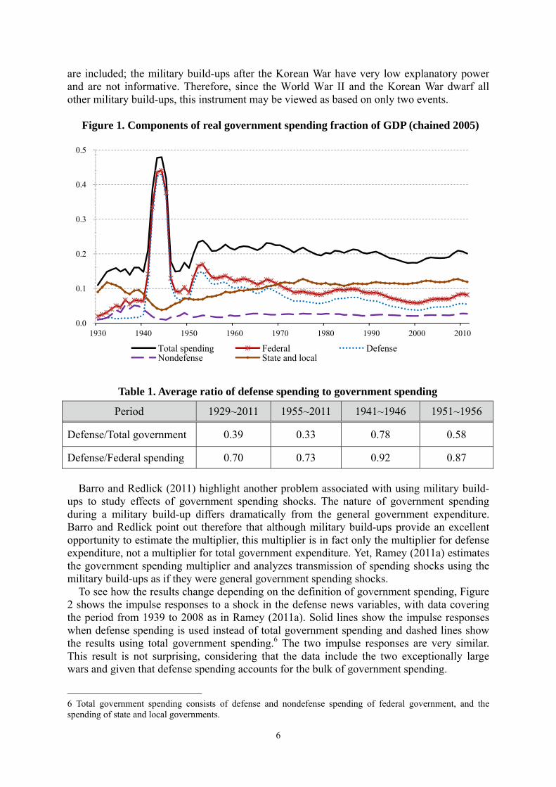
Figure 1 shows the trend of defense and nondefense spending of the federal government and state and local governments, expressed as a ratio to real GDP. The defense spending is a major part of total spending and federal government spending. Especially, the movement of federal government spending is almost perfectly copies of that of defense spending. This is the reasons that much literature chooses the military build-ups as an instrument of government spending shocks.
A potentially important problem with this instrument, however, is that it is dominated by two extraordinarily large events: the World War II and the Korean War. When these are excluded by considering only data after 1955, the ratio of defense spending to GDP displays relatively little variation. Table 1 shows that during World War II and the Korean War, the defense spending accounts for most of the variation in government spending because its ratio to total government spending is much higher than in other periods. Indeed, Ramey (2011a) observes that the military build-ups have explanatory power only when these two large wars
through conscription, and this effect lasted for several years, while the Hurricane Katrina affected 0.3 % of labor force for a few quarters. 4 The fiscal shock associated with Federal government assistance tends to vary considerably across natural disasters, with sometimes similar events resulting in responses of very different magnitudes. For example, although the Californian earthquake of 1994 and the Hurricane Wilma in Florida of 2005 were both estimated to cause similar economic damage (around nominal $20 billion), the assistance from the Federal Emergency Management Agency shows large difference: $6.0 billion for the former and $1.8 billion for the latter. 5 While Ramey and Shapiro (1998) use the Korean War, Vietnam War and the Soviet invasion of Afghanistan, Ramey (2011a) adds also the World War II and 9/11.
6
are included; the military build-ups after the Korean War have very low explanatory power and are not informative. Therefore, since the World War II and the Korean War dwarf all other military build-ups, this instrument may be viewed as based on only two events. Figure 1. Components of real government spending fraction of GDP (chained 2005)
Table 1. Average ratio of defense spending to government spending
Period 1929~2011 1955~2011 1941~1946 1951~1956
Defense/Total government 0.39 0.33 0.78 0.58
Defense/Federal spending 0.70 0.73 0.92 0.87 Barro and Redlick (2011) highlight another problem associated with using military build-
ups to study effects of government spending shocks. The nature of government spending during a military build-up differs dramatically from the general government expenditure. Barro and Redlick point out therefore that although military build-ups provide an excellent opportunity to estimate the multiplier, this multiplier is in fact only the multiplier for defense expenditure, not a multiplier for total government expenditure. Yet, Ramey (2011a) estimates the government spending multiplier and analyzes transmission of spending shocks using the military build-ups as if they were general government spending shocks.
To see how the results change depending on the definition of government spending, Figure 2 shows the impulse responses to a shock in the defense news variables, with data covering the period from 1939 to 2008 as in Ramey (2011a). Solid lines show the impulse responses when defense spending is used instead of total government spending and dashed lines show the results using total government spending.6 The two impulse responses are very similar. This result is not surprising, considering that the data include the two exceptionally large wars and given that defense spending accounts for the bulk of government spending.
6 Total government spending consists of defense and nondefense spending of federal government, and the spending of state and local governments.
0.0
0.1
0.2
0.3
0.4
0.5
1930 1940 1950 1960 1970 1980 1990 2000 2010
Total spending Federal DefenseNondefense State and local

7
Ramey (2011a) analyzes the robustness of her results using a variety of specification such as excluding one of two big events and excluding both. When either the World War II or the Korean War is included, the results are qualitatively similar to those over the full period. However, when she restricts the sample to 1955 to 2008, excluding both large events, the result is qualitatively and quantitatively different. In particular, after a positive defense spending shock, government spending spikes ups only temporally and then turns negative. GDP also rises only on impacts and then its response becomes negative. We also analyze the period from 1975 to 2008, excluding even the Vietnam War. Figure 3 shows the effects of the defense news on the key variables in this case. The government spending increases only on impact and then falls for 5 years, although it is not significantly at conventional levels. The response of GDP is similar to that obtained by Ramey (2011a) when excluding the two large events. Finally, Ramey (2011a) also uses professional forecast errors instead of the defense news shocks for a period from 1968 to 2008 and gets results similar to those for 1955 to 2008 with defense news shocks. Therefore, Ramey’s (2011a) hump-shaped responses of government spending and GDP appear driven by the World War II and the Korean War. The multiplier should therefore be interpreted as a defense spending multiplier.
In addition, Ramey and Shapiro (1998) argue that military build-ups have the advantage that they do not remove private resources except for manufacturing sector. Ramey (2011a) explain that the military spending was financed mostly by issuing debt during the World War II and by taxes during the Korean War. However, it should be noted that the increase of defense spending are financed partly by decreasing allocations to other sectors of government spending such as nondefense and state/local spending. It means that the military build-ups cause a transfer of resources within government sectors. As much literature such as Ilzetzki et al. (2011) and Bénétrix and Lane (2009) shows, the macroeconomic effects of government spending depend on its function. 7 Therefore, when using military build-ups which are concentrated in only defense sector, it is necessary to include the three remaining sectors of government spending among the endogenous variables to gauge the reallocation of funds in the wake of military build-ups.
Figure 2. The effects of defense spending and government spending (1939~2008)
< Government Expenditure > < GDP>
Notes: Solid lines shows the responses with 68% confidential interval band following Ramey’s (2011a)’s specification with defense spending instead of total government spending. The dashed line shows the results of Ramey’s specification with total government spending.
7 According to Bénétrix and Lane (2009), the effects of government spending shocks are different according to the nature of fiscal innovation; shocks to government consumption and shocks to government investment, and the latter has a positive and larger fiscal multiplier.
-3.0
-2.0
-1.0
0.0
1.0
2.0
3.0
4.0
5.0
0 4 8 12 16 20
-0.4
-0.2
0.0
0.2
0.4
0.6
0.8
1.0
0 4 8 12 16 20

8
Figure 2. The effects of defense spending and government spending (1939~2008) (continued)
< 3 month T-bill rate> < Average marginal income tax rate >
< Total hours > < Real wage >
Notes: Solid lines shows the responses with 68% confidential interval band following Ramey’s (2011a)’s specification with defense spending instead of total government spending. The dashed line shows the results of Ramey’s specification with total government spending.
Figure 3. The effects of defense news shocks from 1975 to 2008
< Government Expenditure > < GDP>
Note: A solid line displays point estimates while the dashed lines correspond to 68% confidence interval bands
-15.0
-10.0
-5.0
0.0
5.0
10.0
15.0
0 4 8 12 16 20-0.2
-0.1
0.0
0.1
0.2
0.3
0.4
0 4 8 12 16 20
-0.4
-0.2
0.0
0.2
0.4
0.6
0.8
0 4 8 12 16 20-0.8
-0.6
-0.4
-0.2
0.0
0.2
0.4
0.6
0 4 8 12 16 20
-0.3
-0.2
-0.1
0.0
0.1
0.2
0 4 8 12 16 20-0.3
-0.2
-0.1
0.0
0.1
0 4 8 12 16 20

9
We therefore again apply Ramey’s (2011a) specification and data using defense news, with
the three sectors of total government spending (defense, non-defense and state/local) featuring separately. Figure 4 shows the results. The impulse response of defense spending closely resembles consistent Ramey’s results with a humped shaped pattern. However, we observe large and significant falls in nondefense and state/local spending: the increase in defense spending crowds out the spending in the other two sectors. The responses of other variables such as GDP, real wage and consumption are qualitatively similar to those of Ramey and Shapiro (1998) and Ramey (2011a). This analysis sheds light on the effects of military builds-ups on the total government spending: the increase defense spending is partly counterbalance by decreases in the remaining sectors so that the macroeconomic effects result from compositional responses of government spending sectors.
This again suggests that the multiplier does not reflect the effect of total government spending but applies only to defense spending. It can appear lower than the general government spending multiplier because of the decrease of spending in the other two sectors. Following Ramey (2011a), the implied elasticity of peak GDP to defense spending is 0.047 and the average ratio of GDP to defense spending is 15.2 from 1947 to 2008. The implied defense spending multiplier then is 0.78, which is similar to the defense spending multiplier range (0.6~0.9) found by Barro and Redlick (2011) and that (0.6~0.8) of Ramey (2011a) for the same period. Since this multiplier is calculated with including the effects of crowding out in other government spending sectors, the pure defense spending multiplier, which means that an increase of defense spending is added in total government spending, can be a little higher than this.
Another potential weakness of military build-ups relates to the assumption that they are exogenous and unexpected. Although wars can occur suddenly and unexpectedly, in many cases a military conflict ensues after weeks or months of rising tensions. For instance, the Japanese attack on the US forces in the Pacific in 1941 was unexpected only to the extent that the US expected the Japanese to attack the Philippines (held by the US at the time) rather than Hawaii. Furthermore, once the war has started, it can take several years so that the continued increased spending no longer constitutes a fiscal shock.
Finally, military conflicts, even when they are extra-territorial, do have important supply-side effects: large numbers of young men are conscripted into the armed forces9, firms switch their output towards military-use products and civilian-use physical assets such as trucks, boats and planes can be redirected for military uses such as transporting troops or ordnance.
To sum it up, although military build-ups have several advantages, they rely crucially on infrequent events with an atypical composition of spending. The macroeconomic effects are totally due to the increase of defense spending and the resulting multiplier cannot be representative of the effect of general government spending shocks, but only of changes in defense spending.
8 When we use the average ratio (5.0) of GDP to the total government spending for the same period, the implied defense spending multiplier is 0.23. 9 The number of draftees (the ratio of total labour) accounts for 10.1 million (19.1%) during the World War II, 1.5 million (2.4%) during Korean War, and 1.9 million (2.4%) during Vietnam War respectively.

10
Figure 4. The effects of defense spending shocks from 1947 to 2008
< Defense spending > < Nondefense spending>
< State and local spending> < GDP >
< Real wage > < Private consumption >
Note: A solid line displays point estimates while the dashed lines correspond to 68% confidence interval bands
0.0
1.0
2.0
3.0
4.0
5.0
6.0
0 4 8 12 16 20-4.0
-3.0
-2.0
-1.0
0.0
1.0
2.0
0 4 8 12 16 20
-0.5
-0.4
-0.3
-0.2
-0.1
0.0
0.1
0 4 8 12 16 20-0.3
-0.2
-0.1
0.0
0.1
0.2
0.3
0.4
0 4 8 12 16 20
-1.0
-0.8
-0.6
-0.4
-0.2
0.0
0.2
0.4
0.6
0 4 8 12 16 20-0.4
-0.3
-0.2
-0.1
0.0
0.1
0.2
0.3
0 4 8 12 16 20
11
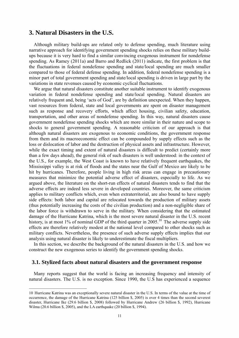
3. Natural Disasters in the U.S. Although military build-ups are related only to defense spending, much literature using
narrative approach for identifying government spending shocks relies on these military build-ups because it is very hard to find a similar convincing exogenous instrument for nondefense spending. As Ramey (2011a) and Barro and Redlick (2011) indicate, the first problem is that the fluctuations in federal nondefense spending and state/local spending are much smaller compared to those of federal defense spending. In addition, federal nondefense spending is a minor part of total government spending and state/local spending is driven in large part by the variations in state revenues caused by economic cyclical fluctuations.
We argue that natural disasters constitute another suitable instrument to identify exogenous variation in federal nondefense spending and state/local spending. Natural disasters are relatively frequent and, being ‘acts of God’, are by definition unexpected. When they happen, vast resources from federal, state and local governments are spent on disaster management such as response and recovery efforts, which affect housing, civilian safety, education, transportation, and other areas of nondefense spending. In this way, natural disasters cause government nondefense spending shocks which are more similar in their nature and scope to shocks to general government spending. A reasonable criticism of our approach is that although natural disasters are exogenous to economic conditions, the government response from them and its macroeconomic effect can be compounded by supply effects such as the loss or dislocation of labor and the destruction of physical assets and infrastructure. However, while the exact timing and extent of natural disasters is difficult to predict (certainly more than a few days ahead), the general risk of such disasters is well understood: in the context of the U.S., for example, the West Coast is known to have relatively frequent earthquakes, the Mississippi valley is at risk of floods and the states near the Gulf of Mexico are likely to be hit by hurricanes. Therefore, people living in high risk areas can engage in precautionary measures that minimize the potential adverse effect of disasters, especially to life. As we argued above, the literature on the short-run effects of natural disasters tends to find that the adverse effects are indeed less severe in developed countries. Moreover, the same criticism applies to military conflicts which, even when extraterritorial, are also bound to have supply side effects: both labor and capital are relocated towards the production of military assets (thus potentially increasing the costs of the civilian production) and a non-negligible share of the labor force is withdrawn to serve in the military. When considering that the estimated damage of the Hurricane Katrina, which is the most severe natural disaster in the U.S. recent history, is at most 1% of nominal GDP of the third quarter in 2005.10 The adverse supply side effects are therefore relatively modest at the national level compared to other shocks such as military conflicts. Nevertheless, the presence of such adverse supply effects implies that our analysis using natural disaster is likely to underestimate the fiscal multipliers.
In this section, we describe the background of the natural disasters in the U.S. and how we construct the new exogenous series to identify the government spending shocks.
3.1. Stylized facts about natural disasters and the government response
Many reports suggest that the world is facing an increasing frequency and intensity of
natural disasters. The U.S. is no exception. Since 1990, the U.S has experienced a sequence
10 Hurricane Katrina was an exceptionally severe natural disaster in the U.S. In terms of the value at the time of occurrence, the damage of the Hurricane Katrina (125 billion $, 2005) is over 4 times than the second severest disaster, Hurricane Ike (29.6 billion $, 2008) followed by Hurricane Andrew (26 billion $, 1992), Hurricane Wilma (20.6 billion $, 2005), and the LA earthquake (20 billion $, 1994).
12
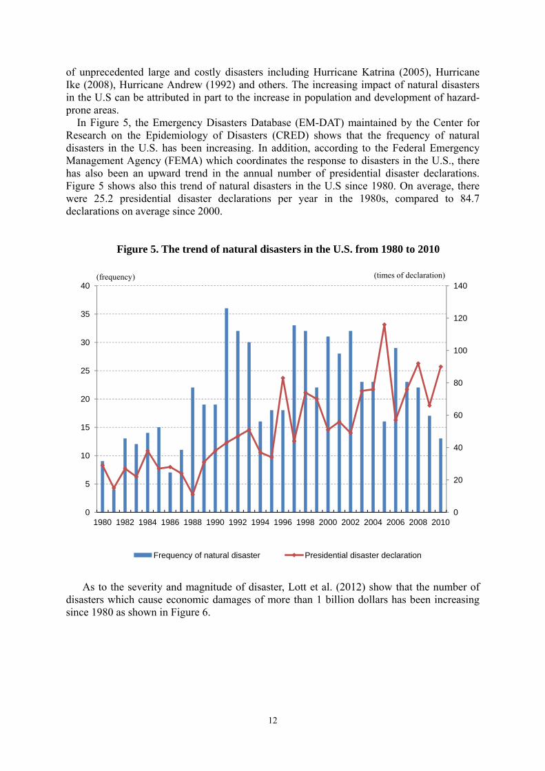
of unprecedented large and costly disasters including Hurricane Katrina (2005), Hurricane Ike (2008), Hurricane Andrew (1992) and others. The increasing impact of natural disasters in the U.S can be attributed in part to the increase in population and development of hazard-prone areas.
In Figure 5, the Emergency Disasters Database (EM-DAT) maintained by the Center for Research on the Epidemiology of Disasters (CRED) shows that the frequency of natural disasters in the U.S. has been increasing. In addition, according to the Federal Emergency Management Agency (FEMA) which coordinates the response to disasters in the U.S., there has also been an upward trend in the annual number of presidential disaster declarations. Figure 5 shows also this trend of natural disasters in the U.S since 1980. On average, there were 25.2 presidential disaster declarations per year in the 1980s, compared to 84.7 declarations on average since 2000.
Figure 5. The trend of natural disasters in the U.S. from 1980 to 2010
As to the severity and magnitude of disaster, Lott et al. (2012) show that the number of disasters which cause economic damages of more than 1 billion dollars has been increasing since 1980 as shown in Figure 6.
0
20
40
60
80
100
120
140
0
5
10
15
20
25
30
35
40
1980 1982 1984 1986 1988 1990 1992 1994 1996 1998 2000 2002 2004 2006 2008 2010
Frequency of natural disaster Presidential disaster declaration
(frequency) (times of declaration)

13
Figure 6. Frequency of disasters with economic damages more than $ 1 billion
Note: Estimated nominal economic damage in 2011 dollars
When a natural disaster happens, the federal government and state and local governments
respond to it cooperatively, following the Federal Response Plan and other applicable laws.11 In the event of a disaster or local emergency, local government has the primary responsibility for responding to, recovering from and mitigating the adverse effects of the disaster. However, when effects of the disaster are beyond the capacity of local resources to respond effectively, the state and federal government assistance is provided through the emergency and disaster declaration process.12 When the declaration for state or federal government is considered, the judgment criteria are mainly based on the damage assessment according to preliminary reports. This means that the state and federal assistance is closely related to the estimated economic damages and as a result, so are the government spending shocks. A presidential disaster declaration triggers action by many federal agencies besides FEMA, including the U.S. Army Corps of Engineers, the Small Business Administration, and the Departments of Agriculture, Transportation, Commerce and others to provide supplemental assistance to state and local governments, families and individuals, and certain nonprofit organizations for mitigation, response and recovery. According to McCarty (2011) of Congressional research service, the amount of assistance provided through presidential disaster declarations to the Gulf coast region in the aftermath of Hurricanes Katrina and Rita has exceeded 140 billion dollars. Major part of this assistance comes from the Disaster Relief Fund (DRE) managed by FEMA as a category of grants-in-aid to state and local governments.13 Under the Stafford Act, many disaster relief costs are to be shared between the federal government and the affected state and local governments. The federal share of funding is at least 75% for public assistance. However, depending on the circumstance, the federal government has raised the federal share for some disasters to as high as 90 % for the 1994 Northridge earthquake and 100% for 1992 Hurricane Andrew (Czerwinski, 1998).
11 For example, there are the Robert T. Stafford Disaster Relief and Emergency Assistance Act (Stafford Act) for federal assistance and Natural Disaster Assistance Act (NDAA) for state assistance. 12 There are three types of declaration: local emergency declaration, Governor’s state of emergency proclamation and Presidential declaration of a federal major disaster or emergency. 13 The Disaster Relief Fund is a “no-year’’ fund managed by the Federal Emergency Management Agency (FEMA) and used only for spending related to presidentially declared disasters. While FEMA budgets are based on the current Fund balance for a given fiscal year (5.8 billion for FY 2008), in a case of its shortage, Congress makes supplemental emergency appropriations as needed to respond to large disasters. (For more information on federal funding for disasters, refer to GAO/RCED-00-182)
0123456789
10
1980 1982 1984 1986 1988 1990 1992 1994 1996 1998 2000 2002 2004 2006 2008 2010
(frequency)
14
3.2. Constructing the natural disaster variable To estimate the effects of government spending shocks on macroeconomics, it is necessary
to identify an instrumental variable which is closely related to government spending shocks but exogenous with respect to the state of the economy. The gravity and impact of natural disasters can be measured with a number of variables, such as the number of persons killed, the number of persons affected or displaced, the estimated economic damage and others. We select the economic damage as an instrumental variable because this is what usually determines the amount of government assistance as explained in the previous subsection. A natural disaster causes government spending shocks in two types: federal nondefense spending and state/local spending which includes the grant from the federal government. In order to reflect this, we proceed in two steps. First, we compile the total economic damages per natural disaster at the national level. Second, the economic damages are allocated to the 50 states used in a panel analysis at the state level.
For the first step, natural disaster list is compiled mainly with major disasters which cause sufficiently large damage to infrastructure, human capital and production facilities that they can exert a substantial effect on government spending. The preliminary disaster list is obtained from EM-DAT because it is a comprehensive database that includes data on the occurrence and effects of over 18,000 mass disasters in the world since 1900. In order to be entered into the EM-DAT database, a disaster must meet at least one of the following criteria: 10 or more people killed; 100 or more people affected; a declaration of a state of emergency; a call for international assistance. We select the period from 1977 to 2009, i.e. after the end of the Vietnam War, in order to minimize contamination of our results by fluctuations of government spending due to military build-ups. We complete this list of major disasters and total economic damages at the national level by cross-checking the EM-DAT database with the lists of presidential major disaster declarations from FEMA and with the list of climate-related disasters with damages exceeding one billion dollars from the National Ocean and Atmospheric Administration (NOAA).
The next step is to distribute the total economic damages per disaster to each state affected. As far as we know, there is no systematic and comprehensive data for this purpose because economic damages at the state-level were not consistently reported. Therefore, we construct a new economic damage series per state from various sources with several criteria applied in sequence.14 The first criterion is the disaster reports by the agencies such as the National Hurricane center, National weather service, and Storm prediction center and others. Most of these reports were written at the time of incidence so they can match better with the government spending shocks which is the variable of interest in this paper. In the case of disasters with no report, we relied on other sources in sequence: the storm event database of the National Climate Data Center;15 EM-DAT; U.S. Geological Survey report; and U.S. Army Corps of Engineers reports. Lastly, for some natural disasters only total damage but no damage data by state is available, we had to distribute it according to the ratio of related data such as financial assistance grant from FEMA, the number of counties where emergency was declared, the number of death and so on. 14 The sources include EM-DAT of CRED, the Storm event database of National climate data center, the National Hurricane center, the National Weather Service, the Federal Emergency Management Agency, U.S. Department of Agriculture, individual state emergency management agencies, state and regional climate centers, Geological Survey reports, U.S. Army Corps of Engineers reports, media reports and insurance industry estimates (Appendix A). 15 The database currently contains data on property and crop damage in millions of dollars from 1996 to present. However, prior to 1996, it shows only range of damage. Therefore, we use the data from this database directly since 1996 but before 1996, we just consult it as a means of the ratio for distributing total economic damages to each state.

15
To analyze the effects of government spending shocks related to natural disasters, it is necessary to transform the constructed economic damages into time series data. At the national level, this requires assigning the calendar dates to quarters. When the natural disaster happens, state government need some time to respond and spend expenditure for relief and recovery efforts due to fiscal policy lags. In case of major natural disasters, in the process of presidential disaster declaration, it takes some times to survey the damaged and destroyed facilities and determine eligibility for assistance. This decision lag for disaster declaration usually takes from 1 week to some months. Therefore, we use the date of the declaration as the date of the associated government spending shock. In addition, even after this declaration, it takes more time for the government to disburse and execute the disaster assistance (implementation lags). We assume that it usually takes about 1 week after the disaster declaration. In order to capture the government spending shock in time, if the disaster declaration occurs in the last week of a quarter, it is assigned to the next quarter16, which is similar to the timing approach of Ramey (2011a).17 On the other hand, for a panel analysis at the state level, since there is no quarterly fiscal data but only annual fiscal data, we allocate the economic damages to fiscal years with a similar way.18 Lastly, we deflate the nominal economic damages using CPI (2005=100).
Figure 7 shows the relation between the economic damages and the corresponding disaster assistance from FEMA at the national level. Data for the size of disaster assistance is available on FEMA website only from 1999 onward. Since other federal agencies and state governments besides FEMA contribute towards the response and repair costs, the disaster assistance from the Disaster Relief Fund is not enough to show the total government spending shocks. However, Figure 7 shows that disaster assistance expenditure occurs in the same quarter as natural disaster or in the following quarter and its size also tracks economic damages of natural disaster similarly. It means that our economic damage series is valid as an instrument for identifying government spending shocks.
Figure 7. The comparison of economic damages and disaster assistance (1999~2009)
16 In case of no declaration for some disasters, if the natural disaster ends during the last week of a quarter, we assign it to next quarter. 17 Appendix A shows the data of our constructed estimated economic yearly damages of natural disasters. 18 In the U.S. while fiscal year of the federal government starts on Oct 1st and ends the following Sep 30th, the fiscal years of the 50 states are different to each other. 46 of the 50 state governments have a fiscal year that runs from July 1st until June 30th. Four states are exceptions: Alabama and Michigan (Oct.1st~Sep.30th), New York (Apr.1st~Mar.31th) and Texas (Sep.1st~Aug.31th).
0
6
12
18
24
30
0
30
60
90
120
150
1999.q1 2000.q1 2001.q1 2002.q1 2003.q1 2004.q1 2005.q1 2006.q1 2007.q1 2008.q1 2009.q1
Economic Damage(left) Disater Assistance(right)
(Billion $) (Billion $)
Disaster Assitance(right)

16
Table 2 shows the basic statistics for disaster damage per state from FY 1977 to FY 2009. In terms of frequency per year, Texas has experienced major disasters more often than any other state, followed by California, Oklahoma, and Louisiana. Although natural disasters occur often in Oklahoma, the damages are small comparatively. On the other hand, the state with the greatest annual damage is Florida with $6.1 billion (not included in the table), followed by Louisiana ($4.5 billion) and California ($2.7 billion).
At the state level, severe disasters can clearly cause massive destructions and labor loss to an affected state as explained in previous section. Therefore, in the section on robustness check, the issue of adverse supply side shocks will be considered.
Table 2. Statistics for disaster damage in Top 5 frequency states
Disaster years
Max damage fiscal year (million, $)
Number of events
Worst disaster (million, $)
Annual damage (million, $)
The U.S. 33 2006 (158,623) 320 Hurricane Katrina
(120,414) 17,449
Texas 30 2009 (22,621) 73 Hurricane Ike
(22,401) 2,057
California 25 1994 (27,032) 61 LA earthquake
(26,220) 2,654
Oklahoma 23 1999 (3,662) 50 Extreme temperature
(2,330) 402
Louisiana 22 2006 (84,923) 41 Hurricane Katrina
(78,682) 4,533
Mississippi 21 2006 (39,778) 37 Hurricane Katrina
(39,194) 2,386
Note: All damages are deflated to chained 2005 dollars and the annual damage means average total damage per state computed with year in which disaster occurred, excluding no disaster years. Disaster years refers to the number of years out of 33 in which at least one disaster occurred. Number of events is the total number of disasters during this period per state.
4. Analysis at the national level
This section presents the macroeconomic effects of government spending shocks related to
natural disasters at the national level of the U.S. To compare our results with other studies using military build-ups, we follow Ramey’s (2011a) methodology, as hers is a representative and recent paper using military-build ups.
4.1. Data and specification We use quarterly U.S. data over the period from 1977 to 2009. As mentioned earlier, this
period is chosen to exclude the Vietnam War (and the previous wars) and thus to minimize the effects of military build-ups. The components of national income and fiscal series are collected in chained (2005) dollars from the NIPA tables of the Bureau of Economic Analysis (BEA). As an interest rate, the 3-month T-bill rate is drawn from the Federal Reserve Bank

17
database (FRB). CPI, hours worked and real wage are taken as an index (2005=100) from the Bureau of Labor Statistics (BLS).19 Population data used to convert the series into per capita terms is drawn from the BEA. All data are seasonally adjusted and nominal values are deflated using the GDP deflator. All variables except the interest rate and economic damage series are expressed in logs of real per capita terms.20
Following other literature including an exogenous variable in an empirical model, our reduced-form VAR model can be expressed as
Xt = A0 + A1t +B(L)Xt−1 +C(L)Dt +εt
where Xt is a vector of endogenous variables, A0 and A1 are the constant term and a linear
trend. B(L) and C(L) are lag polynomials of 4th degree to be consistent with the other literature with quarterly data on fiscal policy. The narrative shocks Dt, economic damages as described in the previous section, is included as the exogenous variable and εt is a vector of reduced-form innovations. The of variables Xt vector consists of federal nondefense spending (Nondef), state/local government spending (State), and federal defense spending (Def), output (GDP), consumer price index (CPI), and short-term interest rate (TB3m). The total government spending is disaggregated into three components because the government spending shocks related to natural disasters rarely affect defense spending which is major part of total government spending:
Xt = (Nondef, State, Def, GDP, CPI, TB3m)′
Other variables of interest such as hours worked, real wage, private consumption and
private investment are then added one at a time as in Burnside et al. (2004). In addition, to identify government spending shocks, the economic damage variable (Dt) is embedded in Xt, but ordered first, following Ramey (2011a)
4.2. Baseline results This subsection presents the impulse responses of the fiscal and macroeconomic variables
to the economic damages as exogenous shocks. The point estimates of impulse response are accompanied by corresponding 68% confidence interval, which is computed by bootstrap standard errors on 1000 replications, like in most previous studies.21 All impulse responses can be interpreted as percentage deviation from a variable’s baseline path, except for those of the interest rate which are reported as deviations from its baseline, measured in percentage points.22
Figure 8 displays the dynamic responses of all variables to a natural disaster shock. The first three graphs show the responses of the three components of government spending. As predicted from the general government response to natural disaster, after a natural disaster shock, the nondefense government spending rises for only 1 year and then return to zero, peaking 2 quarters after the shock. This result explains the federal government response to a
19 Consumer Price Index for All Urban Consumers and All Items, Hours worked index for hours of all persons in nonfarm business sector, and real wage index for real hourly compensation in nonfarm business sector. 20 Appendix B describes the data sources. 21 Many empirical studies on fiscal policy use 68% confidence interval; Ramey (2011), Melecky and Raddatz (2011), Blanchard and Perotti (2002), Burnside et al (2004), and Caldra and Kamps (2008) etc. Additionally, our results with 95% confidence bands are shown in Appendix B. 22 Except for interest rates which percentages points are used for, all response are multiplied by 100 so that a growth rate from the change in log variables is expressed in percent (%).

18
natural disaster well. When a natural disaster occurs, many federal agencies provide supplementary assistance for the initial emergency response for a short period, the cost of which is borne by federal nondefense spending. However, the major part of federal government assistance is the financial assistance from the Disaster Relief Fund, which is grant for state and local governments. Since state and local governments are responsible for the substantial part of relief and repair for a long period, the impulse response of state and local spending should capture this. However, as can be seen in the second graph, its response is not significantly different from zero at all horizons. One plausible explanation is that these grants for several states are too small to be a shock for total state-local spending of the 50 states at the national level. However, it is certain that the affected state government has positive government spending shocks in responding to the natural disaster with its own resources and the federal grant. Therefore, we will deal with this issue in the next section of the cross-state analysis. Defense spending increases a little on impact and then falls insignificantly afterward. The initial short increase can be accounted for the relief and search and rescue efforts of the military including the National Guard. Finally, note that contrary to military build-ups of Ramey (2011a), an increase of nondefense spending does not crowd out the other components of government spending whose responses are insignificant (with the exception of the aforementioned modest and short-lived rise of defense spending).
The response of GDP shows a hump shaped pattern for two years, although it is significant only for one year. It confirms that at the national level, the adverse supply side shocks due to natural disasters are indeed negligible and the effect on GDP results not from the natural disaster itself, but from the government spending that follows it. The implied elasticity of the GDP peak with respect to the nondefense spending is 0.30 and the cumulative elasticity is 0.37 (note that to compute the cumulative elasticity, we consider only four quarters as the effect is not statistically significant thereafter). Since the average ratio of GDP to government spending is 4.7 from 1977 to 2009, the implied nondefense spending multiplier is 1.41 for peak and 1.74 for cumulative effect, which are higher than defense military multiplier (0.6~0.9) of Barro and Redlick (2011) and the multiplier (0.6~1.2) of Ramey (2011a), but is within the range of the peak federal nondefense spending multiplier of 1.0 to 2.5 used by the Congressional Budget Office (2010) for fiscal stimulus packages.23
The next two graphs report the responses of CPI and the interest rate. Although the response of CPI is not significantly different from zero, CPI and the 3-month Treasury bill rate increase after a positive spending shock, which is consistent with the theory.
The fourth and last rows of Figure 8 show the responses of the variables of interest, which as discussed above are added to the model one at a time. Firstly, as to the labor market variables, although their responses are not statistically significant except at the peak, their point estimates are qualitatively consistent with the neoclassical model. The hours worked increase over all horizons after positive government spending shocks and as a result, the response of real wage is negative. Given that government spending is used mainly for repairs and restoration to the original state, labor productivity is not affected24and the decrease of real wage corresponds closely with the increase of hours worked. On the other hand, the response of private consumption is not consistent with the neoclassical model which predicts a negative response of private consumption due to the negative wealth effect. Private consumption increases for 2 years and then falls, following a pattern similar to that of GDP, although it is insignificant. The investment response is large and positive for a long period. It reflects the repair and reconstruction works after a natural disaster. 23 Congressional Budget Office (2010) calculates output peak multiplier by the purchase of goods and service of the Federal government from large macro-econometric models. 24 A comparison of the peak of the hours worked to the peak of the GDP shows that the productivity does not improve.

19
To sum up, a natural disaster causes the federal nondefense spending to increase for one year, but does not affect the other components of government spending at the national level. Based on the response of GDP which is positive significantly for one year after the government spending shocks, the estimated peak nondefense multiplier is 1.41 and the cumulative one is 1.74. The positive response of hours worked and the negative response of real wage is consistent with the neoclassical model. However, private consumption and investment rise for a long period as the government responds to a natural disaster, contrary to the predictions of the neoclassical model.
Figure 8. The effects of government spending shocks
< Federal nondefense spending > < State and local spending >
< Federal defense spending > < GDP >
Note : A solid line displays point estimates while the dashed lines correspond to 68% confidence interval bands
-0.4
-0.2
0.0
0.2
0.4
0.6
0.8
1.0
0 4 8 12 16 20-0.3
-0.2
-0.1
0.0
0.1
0.2
0.3
0.4
0 4 8 12 16 20
-0.8
-0.6
-0.4
-0.2
0.0
0.2
0.4
0.6
0 4 8 12 16 20-0.3
-0.2
-0.1
0.0
0.1
0.2
0.3
0.4
0 4 8 12 16 20

20
Figure 8. The effects of government spending shocks (Continued)
< Consumer Price Index > <3 month T-bill rate >
< Hours worked > < Real wage>
< Private consumption> < Private investment >
Note : A solid line displays point estimates while the dashed lines correspond to 68% confidence interval bands
-0.3
-0.2
-0.1
0.0
0.1
0.2
0.3
0.4
0 4 8 12 16 20-0.3
-0.2
-0.1
0.0
0.1
0.2
0.3
0.4
0 4 8 12 16 20
-0.3
-0.2
-0.1
0.0
0.1
0.2
0.3
0.4
0 4 8 12 16 20-0.3
-0.2
-0.1
0.0
0.1
0.2
0.3
0.4
0 4 8 12 16 20
-0.3
-0.2
-0.1
0.0
0.1
0.2
0.3
0.4
0 4 8 12 16 20-0.8
-0.4
0.0
0.4
0.8
1.2
0 4 8 12 16 20

21
4.3 Robustness checks To check the robustness of the baseline results, this subsection presents several additional
results regarding the usage of three components of government spending and the responses of some variables
4.3.1 Response of total government spending In the baseline analysis, we use three components of total government spending in order to
identify the effects of shocks to nondefense spending. As a robustness check and to produce results more in line with the rest of the literature, we now use the total government spending instead of these components (despite the fact that the natural disaster shocks are rather small compared with the total government spending at the national level).
Figure 9 shows the responses of key variables after total government spending shocks, comparing with the baseline results. Total government spending does not respond significantly to natural disaster shocks. One plausible explanation is that nondefense spending is too small to affect the fluctuation of total government expenditure. With the exception of government spending, the responses of other key variables are qualitatively and quantitatively similar to those of the baseline model.
Figure 9. The effects of total government spending shocks
< Total government spending > < GDP >
< Real wage > < Private consumption >
-0.4
-0.2
0.0
0.2
0.4
0.6
0 4 8 12 16 20Total NondefenseState Defense
-0.3
-0.2
-0.1
0.0
0.1
0.2
0.3
0.4
0 4 8 12 16 20Alternative Baseline
-0.3
-0.2
-0.1
0.0
0.1
0.2
0.3
0 4 8 12 16 20Alternative Baseline
-0.3
-0.2
-0.1
0.0
0.1
0.2
0.3
0 4 8 12 16 20Alternative Baseline

22
4.3.2. The relation between natural disasters and federal defense spending In the baseline result, defense spending responds negatively and strongly after natural
disaster shocks, although this response is not significant. The possible reason is that there is another factor to cause the fall in defense spending, which coincides with the occurrence of natural disasters. Figure 10 shows the trends of defense spending and natural disasters. As explained before, defense spending fluctuated more than other categories of spending due to external factors. Since the end of the Vietnam War, the fluctuation of defense spending has been more modest but still large, mainly reflecting the military build-ups due to the Soviet invasion of Afghanistan (1979) and 9/11 (2001), and the military build-downs due to the end of the Vietnam war (1975) and the collapse of the Soviet Union (1991). Coincidently, big natural disasters such as Hurricane Andrew (1992), LA earthquake (1994), and Hurricane Ike (2008) occurred in the period of military build-downs. As a result, natural disaster seems to cause defense spending to fall statistically.
We perform various checks of the relation between natural disaster and defense spending. Table 3 shows the results. During the military build-up up to 1990, there is no relation between them. However, since 1990, there appears to be a strong negative relationship, which, we argue, reflects the end of the cold war coinciding with increased frequency of natural disasters. In analyzing the fiscal policy with the U.S data, the discretionary fiscal shocks are strongly affected by the fluctuation of defense spending due to its high proportion in total government spending. Further work is needed to explore how to disentangle discretionary nondefense fiscal shocks from defense spending.
Figure 10. The trends of natural disasters and defense spending
Table 3. The relation between natural disaster and defense spending Samples 1977~2009 1977~1990 1990~2009 2000~2009
Correlation -0.22 -0.11 -0.22 -0.42 Coefficient -0.7705*** (0.01) -1.2816 (0.43) -0.6650** (0.05) -0.9103*** (0.01)
Granger-causality Yes*** (0.01) No (0.40) Yes** (0.05) Yes*** (0.01) Notes: Defense spending data is the change from the previous quarter in per capital real defense spending. First, the correlation is for between the 1 lagged value of real economic damage (billion dollars) and the change of defense spending. Second, the coefficient is obtained from a regression of defense spending on 1 lags of the economic damage series. Third, Granger-causality test is done with 1 lags for the hypothesis: Do natural disaster Granger-cause the change of defense spending? Figures in parenthesis refer to P-value.
*** Significant at 0.01 level, **Significant at 0.05 level.
0
100
200
300
400
500
600
700
800
0
20
40
60
80
100
120
140
1977.q1 1980.q4 1984.q3 1988.q2 1992.q1 1995.q4 1999.q3 2003.q2 2007.q1
Dam(left) Defense(right)
(billion $) (billion $)

4.3 As t
consumtheir rethree cois replacinvestm
Figurresponsquantitadisplay falls ansimilar 6 quarteurgentlylater, thin the w
-0.4
-0.3
-0.2
-0.1
0.0
0.1
0.2
0.3
0.4
-0.6
-0.4
-0.2
0.0
0.2
0.4
0.6
.3 Respon
the other lmption and p
sponses andomponents:ced with the
ment is dividre 11 showsses is signifatively and similar res
nd then riseto that of ners and theny after a nat
he responseswake of a na
Figure
0Cons
0
nses of com
literature dprivate inved the speed nondurableese three co
ded into nons the resultsficant at the
qualitativesponses wits sharply o
nonresidentin returns totural disastes of these coatural disast
11. The effe
< Pr
< P
4sumption
4Inves
mponents o
oes, we anestment afted of their ree goods, duomponents onresidential s of this alt
e 68% levelely differenth a hump-sver the coual investme
o zero. In coer and then omponents ter.
ects of com
ivate consum
rivate inves
8Nondurab
stment
23
of consump
nalyze the er governmesponse. Firurable goodone at a timand residen
ternative mo. In terms o
nt from eachshaped patturse of oneent. Residenonsidering tbuy househdepict well
mponents of
mption and
tment and i
8ble goods
8Nonresid
ption and
effects onment spendin
rst, we splids, and servime in the basntial investmodel. Similaof the pointh other. Notern. Howevyear. Intere
ntial investmthat people hold goods a
the actual r
f consumpt
its compone
ts componen
12Durable g
12dential
investmen
n the compng shocks iit private coices. The pseline modement. ar to the bat estimates, ondurable gver, durableestingly, thi
ment increasneed housi
and cars andresponses b
tion and inv
ents >
nts >
16goods
16Resident
nt
ponents of in order to onsumptionrivate consu
el. Similarly
aseline, nontheir respo
goods and e spending is response ses substanting and basd investmen
by the privat
vestment
Services
tial
f private identify
n into its umption
y, private
ne of the nses are services initially is quite
tially for sic items nt goods te sector
20
20

24
4.3.3 The effects of natural disasters except Hurricane Katrina
As in the previous section in which we analyze the effects of military built-ups excluding the World War II and the Korean War, we analyze the response of macroeconomic variables to natural disaster shocks excluding the biggest natural disaster, Hurricane Katrina, which occurred at the end of August 2005. In considering that the GDP responds positively for 8 quarters in the baseline analysis, we exclude two years from 2005.3q to 2007.2q. Figure 12 shows the responses of key variables after total government spending shocks, compared with the baseline. The responses of the three components of government spending when excluding Hurricane Katrina are qualitatively similar to the baseline results. Nevertheless, the magnitude of responses is somewhat smaller and the standard error bands are wider when Hurricane Katrina is omitted. The next graph in Figure 12 shows the response of GDP which rises for one year and then becomes negative after a natural disaster shock. Although it is not significantly different from zero, the elasticity of the GDP peak with respect to the nondefense spending is 0.1 and the average ratio of GDP to government spending is 4.7 for this period. Therefore, the implied multiplier is 0.47 which is much smaller than 1.41 of the baseline analysis because of the small positive response of GDP. It shows that natural disaster series are also dependent on big disasters just like the military build-ups. However, unlike military build-ups, the responses are qualitative similarity regardless of whether big natural disasters are included. Therefore, natural disasters appear a better instrument for identifying unexpected government spending shocks and their effects. The other graphs of Figure 12 also display the responses of key macroeconomic variables when excluding Hurricane Katrina. Along with the response of fiscal variables, the responses of CPI, 3 month T-bill rate, real wage and private consumption qualitatively and quantitatively very similar with and without Hurricane Katrina. In particular, the private consumption rises for one year and then decreases just like GDP. Similarly, the magnitude of the response is smaller than with the full sample. It shows that the response of private consumption follows that of GDP because the private consumption is a major component of GDP.
Figure 12. The effects of government spending shocks excluding Hurricane Katrina
< Federal nondefense spending > < State and local spending >
-0.4
-0.2
0.0
0.2
0.4
0.6
0.8
1.0
0 4 8 12 16 20
Alternative Baseline
-0.4
-0.3
-0.2
-0.1
0.0
0.1
0.2
0 4 8 12 16 20Alternative Baseline

25
Figure 12. The effects of government spending shocks excluding Hurricane Katrina (Continued)
< Federal defense spending > < GDP >
< Consumer Price Index > <3 month T-bill rate >
< Real wage> < Private consumption>
-1.2
-1.0
-0.8
-0.6
-0.4
-0.2
0.0
0.2
0.4
0 4 8 12 16 20Alternative Baseline
-0.4
-0.3
-0.2
-0.1
0.0
0.1
0.2
0 4 8 12 16 20Alternative Baseline
-0.2
-0.1
0.0
0.1
0.2
0.3
0 4 8 12 16 20Alternative Baseline
-0.2
-0.1
0.0
0.1
0.2
0.3
0 4 8 12 16 20
Alternative Baseline
-0.3
-0.2
-0.1
0.0
0.1
0.2
0 4 8 12 16 20
Alternative Baseline
-0.4
-0.3
-0.2
-0.1
0.0
0.1
0.2
0.3
0 4 8 12 16 20
Alternative Baseline
26
5. Cross-state analysis with 50 states
This section presents the macroeconomic effects of state government response after natural disaster shocks using a panel of all 50 states of the U.S. Since the state government spending can be categorized as nondefense spending, the estimates of the effects can shed further light on the nondefense spending multiplier for typical fiscal stimulus packages. In addition, to the best of our knowledge, this analysis is the first attempt to study natural disasters by state.
5.1 Data description
5.1.1. Fiscal and macroeconomic variables
As Ramey (2011a) argues that timing is very important in identifying government spending
shocks, quarterly fiscal data is necessary to obtain precise estimates of the fiscal effect on the economy. However, there are no quarterly fiscal data for all states of the U.S. Therefore, we have to use annual fiscal data. The data on state government expenditure, revenues, and fiscal debts are taken from the U.S. Census Bureau’s Economic Statistics on state government finances, which is available from 1977 to 2009 fiscal years. We use the general fiscal data which means that the expenditure includes all cash payments for goods and services including subsidy, and the revenues consist of all income including intergovernmental revenues such as assistance grant from the federal government during the fiscal year.25 For the state government debt, both short and long term debts are included.
As a state-level output variable, we use personal income instead of gross state product (GSP)26 collected from the U.S. Bureau of Economic Analysis (BEA). The reason is that unlike GSP, personal income data are available at the quarterly frequency and this makes it possible to attribute personal income data to fiscal years. Other state-level variables that we use include the house price index as a proxy for inflation from the Federal Housing Finance Agency (FHFA), and non-farm payroll employment data from the Bureau of Labor Statistics (BLS). The Coincident Economic Activity Index (CEAI), which is set to match the trend for GSP by including four indicators: nonfarm payroll employment, the unemployment rate, average hours worked in manufacturing and wages and salary, is taken from the Federal Reserve Bank (FRB). We obtain total midyear state population data from the Census Bureau. The national consumer price index (CPI) for urban consumers is taken from the BLS.27 All macroeconomic variables are attributed to the appropriate fiscal year in order to match
the fiscal variables. All variables except index variables are in real per capita terms, deflated by the CPI (2005=100). Finally, all variables are expressed in logs.
5.1.2. Properties of the new exogenous instrument Before using the natural disaster damages series as an instrument for government spending
shocks, we check whether these series are unpredicted and exogenous shocks with respect to the state economy and how closely they are associated with discretionary fiscal shocks. First, it can be easily accepted that the occurrence of natural disaster is unexpected and exogenous 25 General expenditure and general revenues comprises all types of expenditure and revenues excepting special accounts: utility, liquor store, and insurance trust. 26 BEA provides only annual GSP data and also GSP has a break in 1997 because of the switch in industry classification from SIC to NAICS. 27 Appendix B describes the data sources.
27
to a state’s economic conditions. Some natural disasters may be expected in disaster-prone areas because they tend to occur during particular times of year. However, this proneness is also irregular and no one can forecast the actual timing and severity of damages.
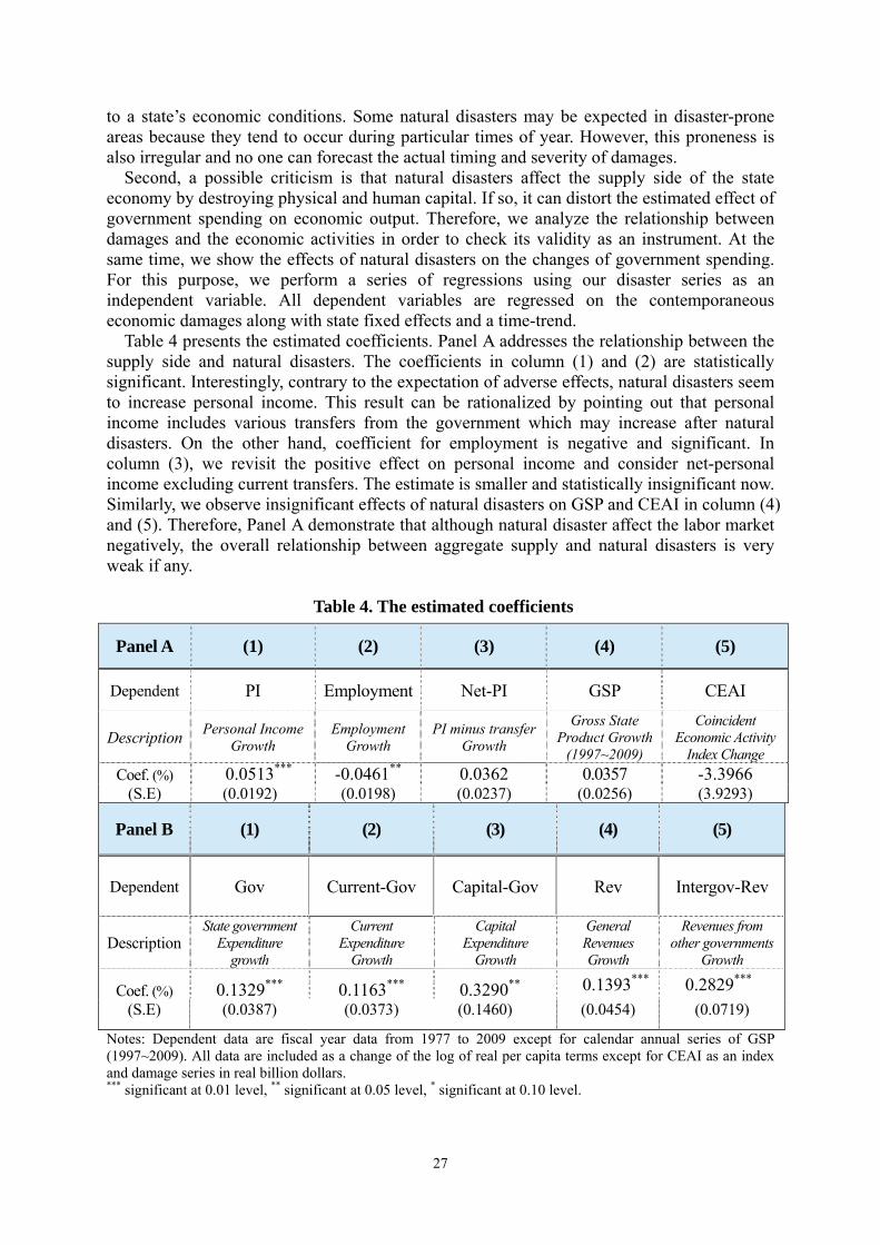
Second, a possible criticism is that natural disasters affect the supply side of the state economy by destroying physical and human capital. If so, it can distort the estimated effect of government spending on economic output. Therefore, we analyze the relationship between damages and the economic activities in order to check its validity as an instrument. At the same time, we show the effects of natural disasters on the changes of government spending. For this purpose, we perform a series of regressions using our disaster series as an independent variable. All dependent variables are regressed on the contemporaneous economic damages along with state fixed effects and a time-trend.
Table 4 presents the estimated coefficients. Panel A addresses the relationship between the supply side and natural disasters. The coefficients in column (1) and (2) are statistically significant. Interestingly, contrary to the expectation of adverse effects, natural disasters seem to increase personal income. This result can be rationalized by pointing out that personal income includes various transfers from the government which may increase after natural disasters. On the other hand, coefficient for employment is negative and significant. In column (3), we revisit the positive effect on personal income and consider net-personal income excluding current transfers. The estimate is smaller and statistically insignificant now. Similarly, we observe insignificant effects of natural disasters on GSP and CEAI in column (4) and (5). Therefore, Panel A demonstrate that although natural disaster affect the labor market negatively, the overall relationship between aggregate supply and natural disasters is very weak if any.
Table 4. The estimated coefficients
Panel A (1) (2) (3) (4) (5)
Dependent PI Employment Net-PI GSP CEAI
Description Personal Income Growth
Employment Growth
PI minus transfer Growth
Gross State Product Growth
(1997~2009)
Coincident Economic Activity
Index Change Coef. (%) 0.0513*** -0.0461** 0.0362 0.0357 -3.3966
(S.E) (0.0192) (0.0198) (0.0237) (0.0256) (3.9293)
Panel B (1) (2) (3) (4) (5)
Dependent Gov Current-Gov Capital-Gov Rev Intergov-Rev
Description State government
Expenditure growth
Current Expenditure
Growth
Capital Expenditure
Growth
General Revenues Growth
Revenues from other governments
Growth
Coef. (%) 0.1329*** 0.1163*** 0.3290** 0.1393*** 0.2829*** (S.E) (0.0387) (0.0373) (0.1460) (0.0454) (0.0719)
Notes: Dependent data are fiscal year data from 1977 to 2009 except for calendar annual series of GSP (1997~2009). All data are included as a change of the log of real per capita terms except for CEAI as an index and damage series in real billion dollars. *** significant at 0.01 level, ** significant at 0.05 level, * significant at 0.10 level.

28
Panel B of Table 4 shows the relevance of our new exogenous variable as an instrument for government spending shocks. In column (1), government spending is significantly related to natural disasters. Columns (2) and (3) confirm that among the two components of government expenditure, capital expenditure is more affected by natural disasters than current expenditure. This is intuitive, given that much of the government response in the wake of natural disasters is concerned with repair and restorations. Columns (4) and (5) show that revenues also increase following natural disasters. This is mainly due to disaster assistance from the federal government which is categorized as the intergovernmental revenues of state governments.
To sum up, economic damages of natural disasters are a strong and relevant instrument for identifying state government spending shocks while they have little if any impact on the supply side of the economy.
5.2. Empirical Analysis
5.2.1. Methodology
To estimate the macroeconomic effects of government spending shocks related to natural
disasters, we formulate a panel vector autoregression (PVAR) model for 50 states of the U.S. during 33 fiscal years from 1977 to 2009. For a given state, the reduced form equation is as follows:
Yi,t = A0 + ∑AjYi,t−j + ∑BjDi,t−j + θi + γit + et , (i : state) (1)
where Yi,t = (Exp, PI, Rev, HPI, Emp)′ is a vector of endogenous variable including government expenditure (Exp), Personal Income (PI), Revenues (Rev), House Price Index (HPI), and Employment (Emp). Di stands for economic damages due to natural disaster as the exogenous variable causing fiscal shocks. θi is a vector of state fixed effects, γi is a vector of state time-trend, and et is a vector of reduced form innovation that is assumed to be independently and identically distributed (i.i.d.). Other variables of interest such as Debt replace Employment one at a time.28 Similar to other studies on the effects of fiscal shocks such as Burnside et al. (2004) and Ramey (2011a), the main identification assumption for estimation is that natural disasters are exogenous and that among the endogenous variables in the vector Yi,t , a variable that comes earlier in the ordering is more exogenous than the ones that appear later.29 In addition, following Ramey (2011a) who embeds the exogenous variable as an endogenous variable in the VAR, we transform the equation (1) and embed the natural disaster variable in the PVAR, but order it first before the other variables:30
Xi,t = A0 + ∑AjXi,t−j + θi + γit + et, where Xi,t = (Di,t′ , Yi,t′ )′ (2)
As suggested by Love and Zicchino (2006), before the equation (2) can be estimated, the original variables need to be time-detrended and the state fixed effects also need to be
28. In many analyses of fiscal policy, additional variables such as the interest rate are often included to control for monetary policy. However, in this baseline specification, such a variable is not included because fiscal policy shocks are observed at the state level, not national level, and the data is annual. 29. This particular ordering is often known as ‘Choleski Ordering’ 30. Ramey (personal communication) argues that the results are similar when the exogenous variable is treated as an exogenous or when it is embeded first in a VAR. We explored both ways with her data and indeed obtained very similar results.

29
eliminated by forward mean-differencing which is known as the ‘Helmet procedure’.31 To check the stationarity of adjusted variables, several panel unit root tests are performed and the results show that all variables are stationary.32 As an optimal lag, 2 annual lags are selected based on the SBIC and HQIC criteria.33
We estimate the equation (2) by using a generalized method of moments (GMM) and then compute the impulse-response function (IRF) to one standard deviation shock of the natural disaster.34. The confidence interval is 68%, obtained using Monte Carlo simulations which generate the 16th and 84th percentiles of the distribution with 1000 repetitions. 35 All responses are multiplied by 100 so that a growth rate from the change in log variables is expressed in percent (%), as in the previous section.
5.2.2. Baseline Results
Figure 13 shows the impulse response functions of fiscal and macroeconomic variables to
fiscal shocks. After a natural disaster happens, the government expenditure follows a hump-shaped pattern, with the response peaking in the second year and remaining significantly positive for 8 years. This confirms that natural disasters are followed by increased government expenditure for relief and repair. Personal income also rises on impact and the response remains significantly positive for 5 years. As shown in the previous subsection, this positive response of personal income suggests that there can be only small adverse supply side effect. The twin peaked pattern of the response of personal income, peaking in years 0 and 2, has two possible interpretations. One is that personal income includes relief transfer to the victims of disasters from the various governments (federal, state and local). This transfer is temporary and short-lived. Subsequently, personal income is positively impacted by the capital reconstruction expenditure which is more persistent. We revisit this issue using alternative income variables that exclude transfer in the next subsection on robustness checks. The other interpretation is that although annual data do not capture the timing of shocks very well, there can be anticipation effects by the private sectors due to time lags of fiscal policy. It means that relief and repair by the private sector can be carried shortly after the disaster, in expectation of government assistance.
In Figure 13, while the elasticity of the personal income peak to the government expenditure peak in the second year is 0.30, the cumulative elasticity for the ten years after the shock is 0.17 (Table 5). Since the average ratio of personal income to government expenditure from 1977 to 2009 is 8.35, the peak income multiplier is estimated at 2.48, but the cumulative one is estimated at 1.45. Interestingly, these income multipliers fall roughly within the range of 1.5 to 3.0 of the other cross-state analyses36, and exceed the range of the U.S aggregate multiplier (0.5~2.0) 37 reviewed by Ramey (2011b) and also our federal 31 According to Love and Zicchino (2006), as the fixed effects are correlated with the regressors due to lags of the dependent variables, the mean-differencing procedure would create biased coefficients. However, forward mean-differencing removes only the forward mean so that it can preserve the orthogonality between transformed variables and lagged regressors 32 We use 6 kinds of unit test in STATA software: Levin-Lin-Chu test, Harris-Tzavalis test, Breitung test, Im-Pesaran-Shin test, Fisher-type tests, Hadri LM stationarity test. 33 Since there is no standard procedure for lag selection under PVAR in STATA, this selection is determined in Eviews. As a robustness check, 1 or 3 lags are also considered. The results are not affected by the number of lags. 34 We consult the STATA package by Love and Zicchino (2006) for this estimation. 35 Results with 90% confidence bands are in Appendix C 36 According to Ramey (2011b), there are around 2 (Shoag, 2010), 0.3~ 3 (Clemens & Miran, 2011), 1.5 (Nakamura and Steinsson, 2011) and 1.88 (Serrato and Wingender, 2011) etc.
37 According to Ramey (2011b), there are 0.6~0.9 (Baro-Redick, 2011), 0.6~1.2 (Ramey, 2011a), 0.9~1.29

30
nondefense spending multiplier (1.41~1.74). Since natural disasters can reduce the productive capacity by destroying physical and
human capital, the multiplier we obtained is likely to be underestimated to a certain degree at the state level. However, in the process of the recovery response, private sector such as insurance companies also plays a significant role in financing repair and reconstruction instead of the government. Therefore, part of output growth can be attributed to the private sector. In this case, the government spending multiplier is likely to be overestimated.38 It is not clear which of these biases is stronger, at any rate, they are likely to partially cancel out.
The next graph shows the response of revenues to the natural disaster shocks. Revenues usually follow the response of output because tax receipts closely depend on the state of the economy. However, in this case, revenues increase on impact, peaking during the first year, i.e. before income peaks. Thereafter, revenues follow a pattern similar to that of personal income and also government expenditure. This suggests that the main source of the change in government revenues (and expenditure) during the first 1~2 years after the disaster is not local taxes, but aid and assistance from the federal government. We explore this further in the analysis of effects on the components of fiscal variables later. Moreover, in the last graph of Figure 13, the response of outstanding government debt supports this interpretation. During 1 year after the shocks, debt responds little and insignificantly. After 2 years, the response of debt is consistent with the pattern of government expenditure. This means that the state government is likely to resort to deficit financing at this time. House price index as a proxy for the price level remains positive and significant for 5 years similar to the response of personal income. Employment initially falls significantly at the time of disaster, as shown in the previous sub-section. However, its response turns positive in the second year and remains significantly positive for 2 years as government expenditure increases.
To summarize, the natural disasters cause positive government expenditure shocks. The response of personal income after the shocks of natural disasters is also positive, peaking after 2 years. The estimated government expenditure multiplier of personal income ranges around between 1.5 and 2.5. The responses of personal income and employment indicate that there are only modest adverse supply side effects. In addition, the increase of the state government expenditure for relief and restoration is financed not from tax revenues but from non-tax sources such as federal government assistance and proceeds from issuance of debt.
Table 5. Cumulative Impacts and Elasticity
Year 0 2 4 6 8 10 Gov growth rate (A, %) 0.31 1.26 1.97 2.30 2.41 2.41 PI growth rate (B, %) 0.14 0.36 0.59 0.60 0.51 0.42 Elasticity (B/A) 0.44 0.28 0.30 0.26 0.21 0.17
(Blanchard-Perotti, 2002), and 1.5 (Fisher-Peters, 2010) etc.
38 To simply estimate pure government expenditure multiplier except the effect from private sector, since the U.S. property damage have been generally estimated by doubling the insured loss reported by the Property Claim Service of the Insurance Services Office, a rough elasticity of personal income to the government expenditure is 0.10(0.16*2/3, peak) or 0.28 (0.42*2/3, cumulative) . In this case, the multiplier can be around between 0.97 ~1.66 and it is likely to be a minimum because it ignores negative effect on output by disasters.

Note: A swhich is
5.3. R In th
verify th
-0.2
0.0
0.2
0.4
0.6
0.8
-0.2
0.0
0.2
0.4
0.6
0.8
-0.2
0.0
0.2
0.4
0.6
0.8
0
< Govern
<
< E
solid line dispsame to all Fi
Robustnes
his subsectihe robustne
0 1 2 3
0 1 2 3
0 1 2 3
Figure nment Expen
< Revenues >
Employment
plays point estigures for resu
ss checks
on, we exaess of the ba
3 4 5 6
3 4 5 6
3 4 5 6
13. Baselinnditure >
>
t >
timates while ults below
amine seveaseline mod
7 8 9
7 8 9
7 8 9
31
ne Results:
the dashed lin
ral alternatdel regarding
10-0.2
0.0
0.2
0.4
0.6
0.8
10-0.2
0.0
0.2
0.4
0.6
0.8
10-0.4
-0.2
0.0
0.2
0.4
0.6
0.8
Impulse-R< P
< H
< G
nes correspon
tive modelsg the assum
0 1 2
0 1 2
0 1 2
Response
Personal In
House Price
Government
nd to 68% con
s with diffemptions and
3 4 5
3 4 5
3 4 5
come >
Index >
t Debt >
nfidence interv
erent variabthe results.
6 7 8
6 7 8
6 7 8
val bands,
bles and First, to
9 10
9 10
9 10
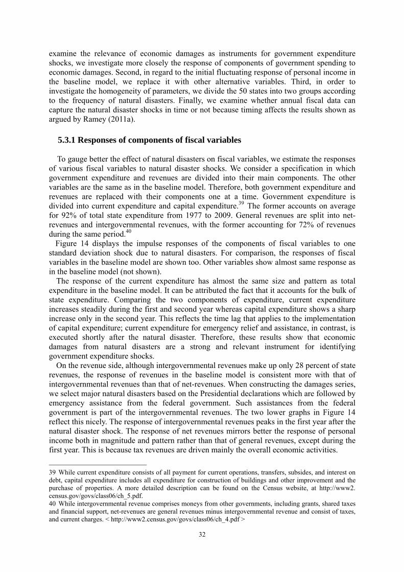
32
examine the relevance of economic damages as instruments for government expenditure shocks, we investigate more closely the response of components of government spending to economic damages. Second, in regard to the initial fluctuating response of personal income in the baseline model, we replace it with other alternative variables. Third, in order to investigate the homogeneity of parameters, we divide the 50 states into two groups according to the frequency of natural disasters. Finally, we examine whether annual fiscal data can capture the natural disaster shocks in time or not because timing affects the results shown as argued by Ramey (2011a).
5.3.1 Responses of components of fiscal variables
To gauge better the effect of natural disasters on fiscal variables, we estimate the responses
of various fiscal variables to natural disaster shocks. We consider a specification in which government expenditure and revenues are divided into their main components. The other variables are the same as in the baseline model. Therefore, both government expenditure and revenues are replaced with their components one at a time. Government expenditure is divided into current expenditure and capital expenditure.39 The former accounts on average for 92% of total state expenditure from 1977 to 2009. General revenues are split into net-revenues and intergovernmental revenues, with the former accounting for 72% of revenues during the same period.40 Figure 14 displays the impulse responses of the components of fiscal variables to one standard deviation shock due to natural disasters. For comparison, the responses of fiscal variables in the baseline model are shown too. Other variables show almost same response as in the baseline model (not shown). The response of the current expenditure has almost the same size and pattern as total
expenditure in the baseline model. It can be attributed the fact that it accounts for the bulk of state expenditure. Comparing the two components of expenditure, current expenditure increases steadily during the first and second year whereas capital expenditure shows a sharp increase only in the second year. This reflects the time lag that applies to the implementation of capital expenditure; current expenditure for emergency relief and assistance, in contrast, is executed shortly after the natural disaster. Therefore, these results show that economic damages from natural disasters are a strong and relevant instrument for identifying government expenditure shocks. On the revenue side, although intergovernmental revenues make up only 28 percent of state
revenues, the response of revenues in the baseline model is consistent more with that of intergovernmental revenues than that of net-revenues. When constructing the damages series, we select major natural disasters based on the Presidential declarations which are followed by emergency assistance from the federal government. Such assistances from the federal government is part of the intergovernmental revenues. The two lower graphs in Figure 14 reflect this nicely. The response of intergovernmental revenues peaks in the first year after the natural disaster shock. The response of net revenues mirrors better the response of personal income both in magnitude and pattern rather than that of general revenues, except during the first year. This is because tax revenues are driven mainly the overall economic activities.
39 While current expenditure consists of all payment for current operations, transfers, subsides, and interest on debt, capital expenditure includes all expenditure for construction of buildings and other improvement and the purchase of properties. A more detailed description can be found on the Census website, at http://www2. census.gov/govs/class06/ch_5.pdf. 40 While intergovernmental revenue comprises moneys from other governments, including grants, shared taxes and financial support, net-revenues are general revenues minus intergovernmental revenue and consist of taxes, and current charges. < http://www2.census.gov/govs/class06/ch_4.pdf >

33
In summary, the responses of components of expenditure and revenues depict the process of government response to natural disasters rather well. On the expenditure side, natural disasters are a good and relevant instrument for government spending shocks. In terms of revenues, a large portion of the increased state government expenditure is financed by the federal government support.
Figure 14. Response of fiscal components to the natural disaster
< Current Expenditure > < Capital Expenditure >
< Intergovernmental Revenues > < Net Revenues >
5.3.2. Alternative measures of personal income
In the baseline model, personal income fails to display the expected hump-shaped response
to the government spending shock. Instead, it increases only on impact. Then, its growth rate falls, only to increase again and remain positive for 5 years, peaking the second year. To
-0.2
0.0
0.2
0.4
0.6
0.8
1.0
1.2
1.4
1.6
0 1 2 3 4 5 6 7 8 9 10
Exp (baseline) Current Exp
-0.2
0.0
0.2
0.4
0.6
0.8
1.0
1.2
1.4
1.6
0 1 2 3 4 5 6 7 8 9 10
Exp (baseline) Capital_Exp
-0.2
0.0
0.2
0.4
0.6
0.8
1.0
1.2
1.4
1.6
0 1 2 3 4 5 6 7 8 9 10
Rev (baseline) Inter_revPI (baseline)
-0.2
0.0
0.2
0.4
0.6
0.8
1.0
1.2
1.4
1.6
0 1 2 3 4 5 6 7 8 9 10
Rev (baseline) Net_revPI (baseline)

34
investigate this more closely, we analyze alternative models including other variables instead of personal income.
First, we replace personal income with net-personal income which is personal income minus personal current transfer receipts. Since personal current transfer receipts include urgent disaster relief benefits, personal income could increase significantly in the year of occurrence. In Figure 15, the first graph shows the response of net-personal income. The responses of all other variables are nearly identical to those of the baseline model (not shown). Interestingly, net personal income displays a hump-shaped response, peaking in the second year just like government expenditure. In addition, after 3 years, its response is also almost the same as that of personal income in both magnitude and pattern. From this analysis, it appears that the initial response of personal income right after the natural disaster is mainly due to the direct government assistance. Then, its response can be mostly attributed to the government expenditure for repair and reconstruction.
Second, we replace personal income with the Coincident Economic Activity Index (CEAI). As this index is complied as a single summary statistic that tracks the current state of the state economy every month by the Federal Reserve Bank, it can be an excellent substitute for personal income or gross state product. The second graph of Figure 15 shows the impulse response of the CEAI. Similarly to the results of the model with net-personal income, responses of all variables except the CEAI are almost the same as those of the baseline model (not shown). As for the CEAI, its response also appears hump-shaped. However, contrary to net-personal income, the response of the CEAI is negative significantly on impact and then increases for 5 years afterwards. Therefore, at the time of the natural disaster, there can be an adverse supply side shock. As the trend for each state’s CEAI is set to match the trend for gross state product, the CEAI includes four indicators: nonfarm payroll employment, the unemployment rate, average hours worked in manufacturing and wages and salaries. These four indicators are all closely related to the situation in the labor market. Not surprisingly then, the response of the CEAI is very similar to that of employment in the baseline model (Figure 13). Although the CEAI is likely to be related to the trend of GSP much more than personal income, personal income seems to be better proxy for output when estimating the effect of government expenditure shocks. The reason is that it can make it possible to calculate an output multiplier and to shed light on the transmission process through the decomposition of personal income.
Third, we now use the time series of gross state product instead of personal income as the output variable.41 As explained in the section on data, using the GSP has some limitations. First, GSP is only available in annual frequency for calendar years. Therefore, it is impossible to match GSP data to fiscal years in which state fiscal variables are reported. Second, there is a break in its series in 1997 because of a change in industry classifications. Therefore, the period from 1997 to 2009 may be too short for PVAR. The bottom graphs of Figure 15 shows the results of the model with GSP. The responses of all variables are qualitatively similar to those of the baseline model (not shown). However, the effects are less precisely estimated in the alternative model. This is especially the case of the response of GSP: it peaks on impact after a natural disaster shock and then falls, remaining positive only by the first year, in contrast to the hump-shaped response of personal income. This difference may be attributed to the limitations of GSP series mentioned above, especially the difference between fiscal and calendar years which makes identifying the shocks more difficult. As the last graph shows, when the responses of GSP are shifted by 1 year backward in the alternative model, the patterns of responses across two models are more similar.
To summarize, replacing personal income with net-personal income, the CEAI and GSP 41 In unreported test, we similarly estimate the effects using the private gross state product (PGSP). The results are almost identical to those of the model with GSP.

helps unet-persvictims of the Cturns pothe persdue to s
5.3.3
In thisgroups,more thstates bgroup.
-0.2
-0.1
0.0
0.1
0.2
0.3
0.4
0
-0.4
-0.2
0.0
0.2
0.4
s understansonal incomrather than
CEAI showositive oncesonal incomsome limitat
Figur
< Net-P
< Gros
3. Frequen
s subsection a high fre
han 15 yearbelong to thTable 6 rep
0 1 2 3Net
0 1 2 3
GSP
nd the initialme shows thn on repair aws that there the gover
me can be thtions of GS
e 15. Respo
Personal Inc
s State Prod
ncy of natu
n, we explorquency gros during 33he high freqports the su
4 5 6PI PI (
3 4 5 6
P
l counterinthat governmand reconstre is a mod
rnment expehe better anP.
onses of alt
ome >
duct >
ural disast
re the robusoup includin years and quency grouummary sta
7 8 9(baseline)
7 8 9
PI (baseline)
35
tuitive respoments spend
ruction, whdest negativenditure incnd adequate
ternative va
< G
ters
tness of ourng states tha low frequup and 30atistics for
10-0.2
-0.1
0.0
0.1
0.2
0.3
0.4
10-0.4
-0.2
0.0
0.2
0.4
onse of persmuch of th
hich only fole supply-sicreases. Thee variable in
ariables to
< Coinciden
Gross State
r results by at experien
uency groupstates are inatural dis
0 1 2
0 1 2
GSP (1
sonal incomhe initial assllows with ade effect oe response n identifyin
personal in
nt Economic (CEAI)>
Product (1
dividing thnced major p with the rincluded in asters acco
3 4 5
CEAI
3 4 5
year backward)
me. The respsistance on a lag. The rn impacts, of GSP sho
ng spending
ncome
Activity Ind
year backwa
he 50 states inatural disaemaining stthe low fr
ording to fre
6 7 8 9
PI (baseline)
6 7 8 9
) PI (ba
ponse of relief to
response but this
ows that g shocks
dex
ard) >
into two asters in tates. 20 equency equency
9 10
9 10
aseline)

36
groups. The frequency of year in the high group is more than two times often than in low group and the average damage is more than three times larger. Therefore, while the baseline model includes 50 states, this subsection focuses on 20 states which are in the high frequency group.
Table 6. Average statistics for disaster per state across frequency groups
Disaster years Number of events Annual damage(million, $)
Total average (50 states) 13.1 (6.50)
22.7 (16.30)
632.1 (1120.69)
High frequency (20 states) 19.5 (3.49)
38.0 (13.33)
1,189.9 (1614.12)
Low frequency (30 states) 8.9 (4.14)
12.5 (7.98)
260.9 (242.51)
Note: ( ) means standard deviation and annual damage denotes the average total damage per state computed only from disaster incidence year, excluding ‘no disaster year’ Table 7 shows the impulse response of key variables to natural disasters in the high
frequency group. When comparing the results with the baseline model of all 50 states, the responses display qualitatively same patterns. However, the magnitudes are much larger than those of the baseline model. This implies that the results obtained in the baseline model are driven largely by natural disasters in the high-frequency group: not surprisingly, given that few natural disasters imply few government spending shocks related to natural disasters. The peak elasticity of personal income to government expenditure is 0.29 and the cumulative elasticity for ten years is 0.09 in the high-frequency group. As the average ratio of personal income to government expenditure from 1977 to 2009 for these 20 states is 8.98, the peak multiplier is estimated to be 2.62 and cumulative multiplier is 0.83. The range of this multiplier is thus a little wider than that of the baseline model (1.45~2.48).
Table 7. Response to the natural disaster and fiscal shocks 0 yr 2 yrs 4 yrs 6 yrs 8 yrs 10 yrs Peak
High frequency groups(20 states) Exp 0.52* 0.83* 0.35* 0.05 -0.04 -0.04 0.83* (2 yrs) PI 0.22* 0.24* 0.07 -0.09* -0.11* -0.09* 0.24* (2 yrs)
Rev 0.62* 0.91* 0.30* 0.03 0.00 0.01 1.07* (1 yr) Emply -0.12* 0.10 -0.02 -0.24* -0.28* -0.20* 0.10 (2 yrs)
Base line(50 states) Exp 0.31* 0.52* 0.30* 0.13* 0.03* -0.01 0.52* (2 yrs) PI 0.14* 0.16* 0.08* -0.02 -0.05* -0.04* 0.16* (2 yrs)
Rev 0.39* 0.56* 0.23* 0.07* 0.02* 0.00 0.67* (1 yr) Emply -0.07* 0.08* 0.05 -0.06* -0.10* -0.08* 0.09* (3 yrs)
Note: An asterisk (*) indicates that 0 is outside 68% confidence interval band. 5.3.4. Timing of natural disasters
As Ramey (2011a) argues, the timing is very important in identifying fiscal policy shocks.
The narrative approach is regarded to have an advantage in regards to the timing if the instrumental variable used is exogenous, unexpected and closely related to government spending. In the baseline analysis, although the natural disaster damage is a strong and relevant instrument, it is hard to identify the government shocks in a timely way because we

37
only have annual fiscal data. Therefore, we explore this issue by considering the timing of natural disasters. First, we transform the natural disaster damage series into a half-fiscal year dataset. Then, we estimate the effects of half yearly data of damages one at a time, replacing the annual damages data in the baseline model. Natural disasters occurring during the first half of a year are more or less certain to cause government expenditure shocks in the current year. However, those in the second half year may not do so because of the fiscal time lag. In this case, it is possible that the government expenditure increases only during the following the year. Table 8 depicts the average statistics for half yearly damage data. The 50 states have similar frequency of major disasters in the first and second half year. However, the average damage, which reflects on the size of government expenditure shocks, it is over two times larger during the first half than in the second half. Therefore, if most large disasters occur during the first half of the fiscal year, the response of government expenditure in the alternative model with the first half-year damage should closely resemble the response of government expenditure in the baseline model well.
Figure 16 shows the responses in the two alternative models along with those of the baseline model. As expected, the responses obtained with the first half year damages are closely consistent with those of baseline model. On the other hand, the responses with the second half-year damages are quantitatively and qualitatively different from those of the baseline model. This mirrors the results obtained with the high and low frequency groups of states: given that large disasters tend to occur during the first half of fiscal year, our results are mainly driven by those observations.
To summarize, in order to check natural disaster’s timing for government expenditure shocks, we estimate the effects with two half-yearly damages data each other. As a result, the responses to the first half yearly damages are consistent with those of fiscal year damages. Therefore, it shows that our damage data catch the timing for government expenditure shocks even in annual fiscal data.
Table 8. Average statistics for the first and the second half yearly damages
Frequency (year) Annual damage (million, $)
Fiscal year 13.1 (6.50)
632.1 (1120.69)
The first half year 7.5 (4.69)
671.2 (1411.22)
The second half year 9.2 (5.64)
290.3 (393.97)
Note: ( ) means standard deviation. All damages cost is deflated in chained 2005 dollars.

38
Figure 16. Alternative models with the first and the second half yearly damages
< Government Expenditure > < Personal Income >
< Revenues > < House Price Index >
< Employment > < Government Debt >
-0.2
0.0
0.2
0.4
0.6
0.8
0 1 2 3 4 5 6 7 8 9 10
First half Second half Year (baseline)
-0.2
0.0
0.2
0.4
0.6
0.8
0 1 2 3 4 5 6 7 8 9 10First half Second half
-0.2
0.0
0.2
0.4
0.6
0.8
0 1 2 3 4 5 6 7 8 9 10
First half Second half
-0.6
-0.3
0.0
0.3
0.6
0.9
0 1 2 3 4 5 6 7 8 9 10First half Second half
-0.2
0.0
0.2
0.4
0.6
0.8
0 1 2 3 4 5 6 7 8 9 10
First half Second half
-0.60
-0.30
0.00
0.30
0.60
0 1 2 3 4 5 6 7 8 9 10First half Second half Year (baseline)
39
8. Conclusions This paper investigates the effects of government spending shocks on key macroeconomic
variables. Many previous empirical studies use military build-ups as an instrument for identifying government spending shocks and estimating the government spending multiplier. However, military build-ups are limited to several events and their effect is largely restricted to the defense sector. Therefore, it is hard to accept that he multiplier obtained with military build-ups represents a general government-spending multiplier.
In order to assess the effect of fiscal policy, it is therefore necessary to have a nondefense spending multiplier. We use natural disasters instead of military build-ups as an instrument for identifying nondefense spending shocks. When a natural disaster happens, government responds by spending resources for relief and repair which are more similar to the general government expenditure than the spending associated with military build-ups. We collect data on natural disasters and the associated economic damages in the U.S. as a new exogenous narrative variable and analyze the response of macroeconomic variables to natural disasters and the corresponding government spending shocks. We carry out this analysis both at the national and state level.
This paper establishes two novel results. First, we show that economic damage due to natural disasters is a strong and relevant instrument for identifying nondefense spending shocks. It matches government spending shocks in time as well as scope, covering general government activities such as housing, construction, education, safety, and welfare transfers. In the analysis of the responses of components of fiscal variables, natural disasters can shed light on the transmission process of government spending. In addition, unlike the military build-ups, it has the advantage that it can be applied easily in other countries.
Second, we calculate two kinds of nondefense multiplier: for federal nondefense spending, with peak/cumulative multipliers estimated as 1.41/1.74 and for state government spending, with the corresponding multipliers 1.45/2.48. These figures fall within the range of multipliers obtained in the previous literature for non-defense spending, while they exceed the defense multipliers such as 0.6~1.2 of Ramey (2011) and 0.6~0.9 of Barro and Redlick (2011). Assuming that federal nondefense spending and state government spending have similar functions, the nondefense multiplier ranges from 1.4 to 2.5
Our paper has several limitations. At the state level, as there is no quarterly data, we have to use annual data. Therefore, it is possible that the timing of government spending shocks is not accurate. Furthermore, while we analyze the effects of government spending shock at the state level, macroeconomic variables of interest such as private consumption and the real wage are not available. These are important from the point of view of differentiating between Neoclassical and New Keynesian theory. As a result, we cannot use our results to confirm the validity of these theoretical models. Further work is needed in order to explore and address these limitations.

40
Appendices
A. The economic damages of natural disasters in the U.S (Billion, $)
Quarter Damage Dam/GDP (%) Quarter Damage Dam/GDP
(%) Quarter Damage Dam/GDP (%)
77.1q 1.00 0.02 88.1q 0.06 0.00 99.1q 1.89 0.02 77.2q 1.49 0.03 88.2q 0.03 0.00 99.2q 2.57 0.02 77.3q 0.90 0.02 88.3q 0.00 0.00 99.3q 3.03 0.03 77.4q 0.27 0.00 88.4q 0.11 0.00 99.4q 7.41 0.07 78.1q 1.96 0.04 89.1q 0.00 0.00 00.1q 0.65 0.01 78.2q 0.00 0.00 89.2q 0.60 0.01 00.2q 2.35 0.02 78.3q 0.49 0.01 89.3q 0.79 0.01 00.3q 1.44 0.01 78.4q 0.33 0.01 89.4q 19.79 0.25 00.4q 2.81 0.02 79.1q 0.00 0.00 90.1q 0.24 0.00 01.1q 3.11 0.03 79.2q 2.61 0.04 90.2q 0.76 0.01 01.2q 8.47 0.07 79.3q 6.14 0.10 90.3q 0.00 0.00 01.3q 0.02 0.00 79.4q 0.59 0.01 90.4q 0.05 0.00 01.4q 0.05 0.00 80.1q 0.87 0.01 91.1q 5.58 0.07 02.1q 0.46 0.00 80.2q 3.49 0.06 91.2q 0.90 0.01 02.2q 2.19 0.02 80.3q 6.28 0.11 91.3q 3.88 0.05 02.3q 2.14 0.02 80.4q 0.00 0.00 91.4q 3.91 0.05 02.4q 2.26 0.02 81.1q 0.00 0.00 92.1q 1.32 0.02 03.1q 0.51 0.00 81.2q 0.96 0.02 92.2q 0.25 0.00 03.2q 6.60 0.06 81.3q 0.98 0.02 92.3q 39.37 0.47 03.3q 4.20 0.04 81.4q 0.24 0.00 92.4q 3.31 0.04 03.4q 2.55 0.02 82.1q 0.71 0.01 93.1q 7.43 0.09 04.1q 0.00 0.00 82.2q 1.75 0.03 93.2q 1.56 0.02 04.2q 1.25 0.01 82.3q 0.12 0.00 93.3q 15.56 0.18 04.3q 39.65 0.32 82.4q 1.28 0.02 93.4q 0.87 0.01 04.4q 7.09 0.06 83.1q 1.72 0.03 94.1q 31.15 0.36 05.1q 1.35 0.01 83.2q 1.50 0.02 94.2q 0.82 0.01 05.2q 0.37 0.00 83.3q 3.93 0.06 94.3q 0.61 0.01 05.3q 128.32 1.01 83.4q 1.04 0.02 94.4q 1.47 0.02 05.4q 16.45 0.13 84.1q 0.19 0.00 95.1q 3.71 0.04 06.1q 0.52 0.00 84.2q 5.48 0.08 95.2q 5.27 0.06 06.2q 2.03 0.02 84.3q 0.76 0.01 95.3q 1.31 0.01 06.3q 1.02 0.01 84.4q 0.00 0.00 95.4q 4.52 0.05 06.4q 0.36 0.00 85.1q 2.24 0.03 96.1q 1.74 0.02 07.1q 0.90 0.01 85.2q 1.36 0.02 96.2q 0.27 0.00 07.2q 1.20 0.01 85.3q 2.39 0.03 96.3q 5.02 0.05 07.3q 0.59 0.00 85.4q 7.40 0.11 96.4q 0.26 0.00 07.4q 1.90 0.01 86.1q 0.79 0.01 97.1q 3.46 0.04 08.1q 1.43 0.01 86.2q 0.05 0.00 97.2q 6.10 0.06 08.2q 3.31 0.02 86.3q 1.26 0.02 97.3q 0.52 0.01 08.3q 2.66 0.02 86.4q 0.00 0.00 97.4q 0.03 0.00 08.4q 14.85 0.12 87.1q 0.00 0.00 98.1q 3.24 0.03 09.1q 0.48 0.00 87.2q 0.28 0.00 98.2q 3.53 0.03 09.2q 0.73 0.01 87.3q 0.26 0.00 98.3q 8.05 0.08 09.3q 0.23 0.00 87.4q 0.57 0.01 98.4q 2.37 0.02 09.4q 0.13 0.00
** Damages are expressed in real terms using the CPI (2005=100)

41
B. Data Appendix
1. Natural disaster Data Source Website
Disaster list Emergency Disaster Database (CRED) http://www.emdat.be
Federal disaster declaration list
Federal Emergency Management Agency (FEMA) http://www.fema.gov/disasters
Billion $ disaster list National Climate Data Center http://www.ncdc.noaa.gov/billions
Disaster damages report National Hurricane Center http://www.nhc.noaa.gov
Disaster damages report National Weather Service http://www.weather.gov
Disaster damages report Storm prediction center http://www.spc.noaa.gov
Storm Events Database National Climate Data Center http://www.ncdc.noaa.gov/stormevents
2. National level
Series Source Description
Government spending NIPA Table 1.1.5. (BEA) Nominal series deflated by GDP deflator GDP, Consumption, Investment NIPA Table 1.1.6. (BEA) Real series, chained (2005) dollars
Consumer Price Index Price database (BLS) All urban consumer and all items (1982-84=10)
3-month Treasury Bill Economic data (FRB) Seasonally adjusted using X-12 ARIMA
Hours worked Productivity database (BLS) All person in nonfarm business sector, index (2005=100)
Real wage Productivity database (BLS) Real hourly compensation in nonfarm business sector, index (2005=100)
Population NIPA Table 2.1 (BEA) Mid-period and seasonally adjusted
3. State level
Series Source Description
Government expenditure State government finance (CB) Nominal series deflated by CPI
Revenues State government finance (CB) Nominal series deflated by CPI
Personal income Regional data (BEA) Nominal series deflated by CPI
House price index State HPI data (FHFA), Economic data (FRB) Index (2005=100)
Employment Employment database (BLS) Non-farm payroll, Quarterly data
Government debt State government finance (CB) Nominal series deflated by CPI
Gross state product Regional data (BEA) Real series, chained (2005) dollars Coincident Economic Activity Index U.S. regional data (FRB) Index (1992=100)
State population Population estimates (BEA) Midyear, historical data

42
B. 68% and 95% confidence bands of the results at the national level
< Federal nondefense spending > < State and local spending >
< Federal defense spending > < GDP >
< Consumer Price Index > <3 month T-bill rate >
-0.6
-0.3
0.0
0.3
0.6
0.9
1.2
0 4 8 12 16 20
-0.4
-0.2
0.0
0.2
0.4
0 4 8 12 16 20
-1.2
-0.9
-0.6
-0.3
0.0
0.3
0.6
0 4 8 12 16 20-0.4
-0.2
0.0
0.2
0.4
0.6
0 4 8 12 16 20
-0.2
-0.1
0.0
0.1
0.2
0.3
0.4
0 4 8 12 16 20 -0.2
-0.1
0.0
0.1
0.2
0.3
0.4
0 4 8 12 16 20
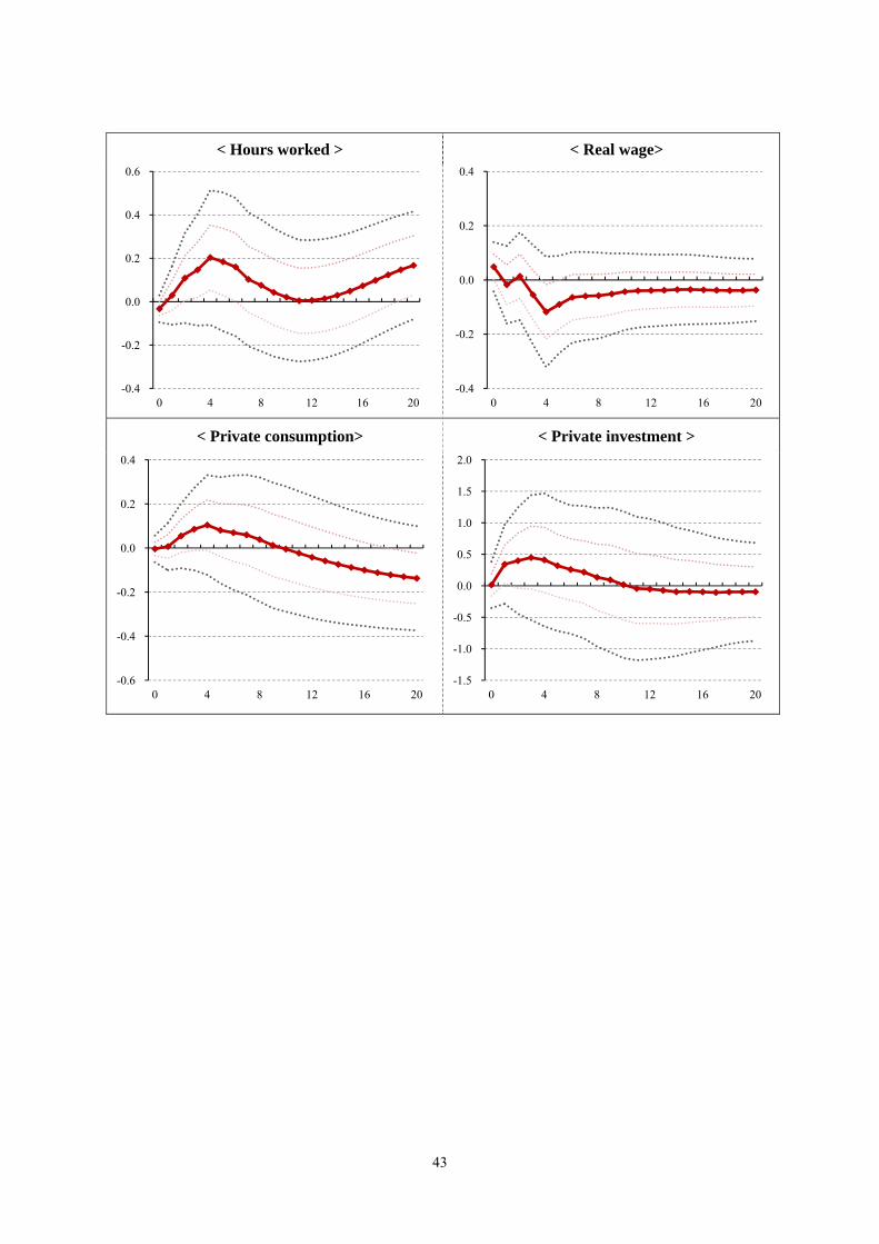
43
< Hours worked > < Real wage>
< Private consumption> < Private investment >
-0.4
-0.2
0.0
0.2
0.4
0.6
0 4 8 12 16 20-0.4
-0.2
0.0
0.2
0.4
0 4 8 12 16 20
-0.6
-0.4
-0.2
0.0
0.2
0.4
0 4 8 12 16 20-1.5
-1.0
-0.5
0.0
0.5
1.0
1.5
2.0
0 4 8 12 16 20
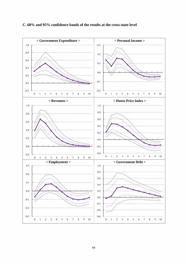
44
C. 68% and 95% confidence bands of the results at the cross-state level
< Government Expenditure > < Personal Income >
< Revenues > < House Price Index >
< Employment > < Government Debt >
-0.2
0.0
0.2
0.4
0.6
0.8
1.0
0 1 2 3 4 5 6 7 8 9 10-0.2
-0.1
0.0
0.1
0.2
0.3
0 1 2 3 4 5 6 7 8 9 10
-0.2
0.0
0.2
0.4
0.6
0.8
1.0
0 1 2 3 4 5 6 7 8 9 10
-0.4
-0.2
0.0
0.2
0.4
0.6
0.8
1.0
0 1 2 3 4 5 6 7 8 9 10
-0.3
-0.2
-0.1
0.0
0.1
0.2
0.3
0 1 2 3 4 5 6 7 8 9 10-0.6
-0.4
-0.2
0.0
0.2
0.4
0.6
0.8
1.0
0 1 2 3 4 5 6 7 8 9 10

45
References
Barro, R., and Redlick, C. (2011), “Macroeconomic effects from government purchases and taxes”, Quarterly Journal of Economics, 126, 51-102.
Bénétrix, A., and Lane, P. (2009), “The impact of fiscal shocks on the Irish economy”, Economic and Social Review, 40, 407-434. Blanchard, O., and Perotti, R. (2002), “An empirical characterization of the dynamic effects of changes in government spending and taxes on output”, Quarterly Journal of Economics, 119, 1329-1368.
Burnside, C., Eichenbaum, M. and Fisher, Jonas D.M. (2004), “Fiscal shocks and their consequence”, Journal of Economic Theory, 115, 89-117.
Cavallo, E., and Noy, I. (2010), “The economics of natural disasters- A survey”, IDB working paper, 124.
Congressional Budget Office (2010), “Estimated impact of the American recovery and reinvestment act on employment and economic output from October 2009 through December 2009”, CBO report 4136. Crespo Cuaresma, J., Hlouskova, J., and Obersteiner, M. (2008), “Natural disasters as creative destruction? Evidence from Developing Countries”, Economic Inquiry, 46, 214-226. Czerwinski, S. J. (1998), “Disaster assistance: Information on Federal costs and approaches for reducing them”, U.S. Accounting Office’s report. Fishback, Price V., and Kachanovskaya, V. (2010), “In search of the multiplier for federal spending in the states during the new deal”, NBER working paper, 16561. Giordano, R., Momigliano, S., Neri, S., and Perotti, R. (2007), “The effects of fiscal policy in Italy: Evidence from a VAR model”, European Journal of Political Economy, 23, 707-733. Ilzetzki, E., Mendoza, E. G., and Végh, C. A. (2011), “How big (small?) are fiscal multipliers?”, IMF working paper 11/52. Lis, E. M., and Nickel C. (2009), “The impact of extreme weather events on budget balances and implications for fiscal policy”, European Central Bank working paper, 1055. Loayza, N., Olaberría, E., Rigolini, J., and Christiaensen, L. (2009), “Natural disaster and growth –going beyond the averages”, World Bank Policy Research Working Paper, 4980. Lott, N., Smith, A., Houston, T., Shein, K., and Crouch, J. (2012), “Billion Dollar U.S. Weather/Climate Disasters, 1980-2011”, National Climatic Data Center (http://www.ncdc.noaa.gov/oa/reports/billionz.html). Love, I., and Zicchino, L. (2006), “Financial development and dynamic investment behavior:

46
evidence from panel VAR”, Quarterly Review of Economics and Finance, 46, 190-210. Melecky, M., and Raddatz, C. (2011), “How do governments respond after catastrophes? Natural disaster shocks and the fiscal stance”, World Bank Policy Research working paper, 5564. McCarthy, Francis X. (2011), “FEMA’s Disaster Declaration Process: A Primer”, CRS reports for Congress, 7-5700. Nakamura, Emi, and Steinsson, Jón (2011), “Fiscal stimulus in a monetary union: Evidence from U.S. regions”, Columbia University working paper, March. Noy, I. (2009), “The macroeconomic consequence of disasters”, Journal of Development Economics, 88, 221-23.1. Noy, I., and Nualsri, A. (2011), “Fiscal storms: public spending and revenues in the aftermath of natural disasters”, Environment and Development Economics, 16, 113-128. Perotti, R. (2005), “Estimating the effects of fiscal policy in OECD countries”, CEPR discussion paper, 4842. Raddatz, C. (2007), “Are external shocks responsible for the instability of output in low-income countries?”, Journal of Development Economics, 84, 155-187. Raddatz, C. (2009), “The wrath of God: Macroeconomic costs of Natural disasters”, World Bank Policy Research working paper, 5039. Serrato, Juan C. S., and Wingender, P. (2010), “Estimating local fiscal multipliers”, Berkeley working paper, November. Shoag, Daniel (2010), “The impact of government spending shocks: Evidence on the multiplier from state pension plan returns”, Job Market Paper. Skidmore, M., and Toya, H. (2002), “Do natural disasters promote long-run growth?”, Economic Inquiry, 40(4), 664-687. Ramey, V. A., and Shapiro, M. D. (1998), “Costly Capital Reallocation and the Effects of Government Spending”, Carnegie-Rochester Conference Series on Public Policy, 48, 145- 194.
Ramey, V. A. (2011a), “Identifying government spending shocks: it’s all in the timing”, Quarterly Journal of Economics, 126, 1–50.
Ramey, V. A. (2011b), “Can government purchase stimulate the economy?” Journal of
Economic Literature, 49:3, 673-685.