THESIS FOR THE DEGREE OF DOCTOR OF PHILOSOPHY

The impact of wind power variability on the least-cost dispatch of units in the electricity generation system

LISA GÖRANSSON

Department of Energy and Environment

CHALMERS UNIVERSITY OF TECHNOLOGY

Gothenburg, Sweden 2014

The impact of wind power variability on the least-cost dispatch of units in the electricity generation system LISA GÖRANSSON ISBN 978-91-7597-001-1 © LISA GÖRANSSON, 2014. Doktorsavhandlingar vid Chalmers tekniska högskola Ny serie nr 3682 ISSN 0346-718X Department of Energy and Environment Chalmers University of Technology SE-412 96 Gothenburg Sweden Telephone + 46 (0)31-772 1000 Chalmers reproservice Gothenburg, Sweden 2014

The impact of wind power variability on the least-cost dispatch of units in the electricity generation system LISA GÖRANSSON Department of Energy and Environment Chalmers University of Technology Abstract This thesis investigates the dynamics of electricity generation systems that involve high levels of wind power. Methods to account for wind power variability in electricity-dispatch models are explored, and the impact of wind power variability on the optimal output of the generation units, so as to meet the system load with the lowest possible cost (economic dispatch), is analyzed for several systems, for both regional and European cases. Systems that lack active variation management, as well as systems with variation management through storage, charging of plug-in hybrid electric vehicles, and trade with the hydropower-rich Nordic countries, are investigated. The work considers systems in which wind power supplies between 20 % and 40 % of the electricity demand on an annual basis.

From the work of this thesis, it is concluded that the inclusion of cycling costs can have significant impacts on the capacity factor of individual generation units obtained from modeling the regional dispatch of systems with 20 % wind power penetration (i.e., annual wind power generation relative to annual demand for electricity). Whether cycling costs need to be included in the systems analysis depends on the wind penetration level and the research question being posed, as well as the relationship between the cycling costs and running costs of the thermal units in the system.

Furthermore, it is shown that in a wind-thermal system, in which wind power generation corresponds to about 20% of the demand for electricity, the variations in net load (here defined as the demand for electricity reduced by wind power generation each hour) follow a diurnal pattern, and load shifting from day to night reduces the competition between wind power and thermal generation with poor cycling properties. However, in systems with about 40% wind power, the ability to store electricity or to shift the load over longer time periods (i.e., several days) confers significant advantages compared to load shifting from day to night, owing to the altered pattern of the variations in net load.

Finally, this thesis shows that the role of the Nordic electricity-generation system in the European context relies heavily on the balance between investments in interconnector capacity and investments in Nordic generation capacity. If planned interconnections between Norway and the rest of Europe are established, net export of electricity is likely from the Nordic countries to Germany and the UK, whereby hydropower-rich Norway would play a central role in redistributing electricity from high-wind events to peak-load events.

Keywords: Wind power, intermittency, variability, dispatch modeling, variation management, electricity generation system, wind-thermal system, cycling costs

List of papers

This thesis is based on the following appended papers:

I. Dispatch modeling of a regional power generation system - Integrating wind power L. Göransson and F. Johnsson, Renewable Energy (2009), 34 (4) pp. 1040–1049

II. Large scale integration of wind power: moderating thermal power plant cycling L. Göransson and F. Johnsson, Wind Energy (2011), 14 (1) pp. 91–105

III. Integration of plug-in hybrid electric vehicles in a regional wind-thermal power system L. Göransson, S. Karlsson and F. Johnsson, Energy policy (2010), 38 (10) pp. 5482–5492

IV. Cost-optimized allocation of wind power investments: a Nordic-German perspective L. Göransson and F. Johnsson, Wind Energy (2013), 16 ( 4 ) pp. 587–604

V. Linkages between demand-side management and congestion in the European electricity transmission system L. Göransson, J. Goop, T. Unger, M. Odenberger and F. Johnsson, Accepted for publication in Energy

VI. The role of Nordic hydropower to handle variations in the future European electricity system L. Göransson, J. Goop, M. Odenberger and F. Johnsson, Proceedings of the 12th Wind Integration Workshop (2013), 22-24 October, London, UK, pp. 293–297

Lisa Göransson is the main author of all six papers and conducted the modeling for these papers. Joel Goop contributed to the analysis and writing of Papers V and VI. Sten Karlsson, Thomas Unger, and Mikael Odenberger contributed to the discussion and to the editing of Papers III, V, and VI, respectively. Filip Johnsson contributed to the discussion and editing of all the papers.

Content 1 Introduction ................................................................................................................................. 1

1.1 Background ......................................................................................................................... 1

1.2 Aim and research questions ................................................................................................. 2

1.3 Outline of this thesis ............................................................................................................ 3

2 Scope and related work ............................................................................................................... 3

2.1 Scope and limitations .......................................................................................................... 3

2.2 Related work ....................................................................................................................... 5

2.3 Contribution of this thesis ................................................................................................... 9

2.4 Model overview ................................................................................................................. 10

2.5 Brief overview of the appended papers ............................................................................. 13

3 Methodology ............................................................................................................................. 15

3.1 Models applied in this thesis ............................................................................................. 15

3.1.1 Stand-alone regional model ....................................................................................... 15

3.1.2 BALMOREL ............................................................................................................. 15

3.1.3 EPOD ......................................................................................................................... 16

3.1.4 ELIN .......................................................................................................................... 17

3.2 Methods to account for wind power variability in dispatch models ................................. 17

3.2.1 General formulation of a dispatch model .................................................................. 19

3.2.2 Three ways to account for the flexibility-related properties of thermal generation .. 20

3.2.3 Time resolution and temporal scope .......................................................................... 33

3.2.4 Variation management strategies ............................................................................... 35

3.2.5 Modeling electricity exchange ................................................................................... 40

3.2.6 The impact of the unpredictability of wind power on the dispatch ........................... 47

4 Conclusions and Discussion ..................................................................................................... 49

4.1 The impact of wind power variability on the dispatch of thermal generation................... 49

4.2 Variation management ...................................................................................................... 51

4.3 The relationship between the Nordic electricity generation systems and the rest of Europe ……………………………………………………………………………………………52

5 Future work ............................................................................................................................... 53

6 References ................................................................................................................................. 54

Acknowledgements

Thanks to Thomas Unger, Mikael Odenberger, and Hans Ravn for sharing your models and your profound knowledge of modeling electricity generation systems. You let me take your time even when I, as a master’s degree student, was completely new to systems modeling and GAMS. Without your help, I would have been lost.

Thanks to Filip Johnsson for your apropos questions, which on more than one occasion have made me realize that some aspect deserves to be scrutinized. In addition, thank you for your patience. I have been on three periods of parental leave between my licentiate thesis and dissertation and this has not drawn as much as a sigh from you.

Thanks to Joel Goop for the fantastic collaboration on Papers V and VI. Logical reasoning is as natural to you as breathing.

Thanks to Tuan Le for answering my questions regarding power flows in the transmission grid. If your day was fully booked you would meet me over lunch!

Thanks to Ulrika Claeson-Colpier and Thomas Unger for patiently reading and commenting upon this summarizing chapter, as well as for encouragement throughout the writing of this thesis.

Thanks to my colleagues at the Department of Energy and Environment at Chalmers for broadening my perspective. Your interest in my research motivates me in my daily work.

Thanks to Jonas and Ville, Simon and Lukas. While you may take time from my work, without you this thesis would never have spanned as many dimensions. Parental leave is also a time for reflection. I love you.

1

1 Introduction

1.1 Background In 2010, electricity generation accounted for 41% of the annual global emissions of carbon dioxide (CO2) from fuel combustion (IEA, 2012a). Thus, to reduce the impact on global climate of human activities, significant restructuring of electricity generation systems is required. Wind power is often identified as a key technology in the drive towards a more sustainable electricity generation system. Currently, approximately 300 GW of wind power is installed around the world (GWEC, 2013). This level is expected to increase to around 1700 GW by 2035 (IEA, 2012b). By then, wind power will provide 14% of the world’s total electricity generation (IEA, 2012b). Due to large difference in conditions for wind power generation, it is likely that wind penetration levels in some parts of the world will be much higher than the global average.

Wind power differs from thermal generation in two important aspects: 1) it is associated with low running costs; and 2) it involves a level of electricity generation that varies depending on external elements (i.e., wind conditions). Due to its low running cost, there are strong economic incentives for the employment of wind power to supply the electricity demand once the wind power capacity has been put in place. However, the share of the load that can be supplied by wind power for a specific hour not only depends on the characteristics of the load and installed capacity, but also on prevailing wind speeds.

At present, electricity generation is based mainly on the combustion of fossil fuels. For fossil-fueled power plants, there is a trade-off between low running costs and flexibility. For example, large coal-fired power plants have low running costs but high start-up costs, whereas gas turbines have low start-up costs but high running costs. The electricity generation system is currently designed to manage the diurnally recurring load variations, so that there are power-generating units with low running costs to cover the demand for electricity which is continuous throughout the week whereas more flexible units with higher running costs meet the peak demand for electricity during working hours. Thus, running costs and the flexibility to follow load determine the dispatch of the electricity-generating units in the system. Since load variations follow a regular diurnal pattern, the period of time and extent to which each unit will supply the thermal system with power are known.

In contrast to load variations, wind power variations follow no specific pattern. Thus, in a wind-thermal power system, the combination of units that can supply the system with electricity at the lowest cost depends on the level of wind power generation and the load for that particular hour. Since there is a substantial cost associated with starting fossil-fueled power plants, the optimal combination must also reflect the levels of wind power generation and load several hours back in time as well as ahead in time.

Since fossil-fuelled power plants with low running costs typically are inflexible and are most efficient when operated continuously at rated power, there is an economic incentive for reducing

2

variations in the electricity generation system. Due to boundary conditions and the model setup, regional studies often give an export of variations in wind power generation to regions that lies outside the scope of the modeled system (for examples, see the work of Holttinen and Pedersen (2003), as well as Paper I in this thesis), and variations in wind power generation may indeed be reduced as the geographic scope increases (Holttinen et al., 2011). However, the extent to which variations can be managed by transmission and trade obviously depends on the transmission system in place, as well as the electricity system at the other end of the transmission line. Variations can also be reduced by adding active variation management, in the form of storage capacity or demand-side management (DSM) to the electricity system.

1.2 Aim and research questions The purpose of this thesis is to define and develop methods and models in order to analyze the impact of wind power variability on the economic dispatch of a given electricity generation system, i.e., the optimal output from electricity generation units to meet the system load at the lowest possible cost. The work seeks to refine and develop primarily existing dispatch models, so as to improve their abilities to analyze electricity generation systems that comprise high levels of wind power. The purpose of the research undertaken in this thesis is to address the same questions that are traditionally posed to dispatch models, but to do this in the case of there being substantial wind generation present in the modeled system. Dispatch models are expected to provide information regarding: total system running costs; the marginal costs to generate electricity; electricity trade volumes and trading patterns; full-load hours for different technologies; the fuel mix of the system; and the levels of CO2 emissions from electricity generation. The work has been carried out within a research group that investigates scenarios for the development of the European electricity generation system within the restriction of strict climate targets. In this context, the impacts of wind power variability, which may influence investment decisions, which include the full-load hours of different generation technologies in different system contexts (i.e., with and without storage, DSM etc.), are of particular interest.

To analyze systems that incorporate high levels of wind power, an understanding of the interactions between wind power and other generation units in the system is needed. The addition of active variation management (such as storage or DSM) can change the ways in which different units in the system interact, and there is a need to understand how the different properties of the variation management strategy influence system dynamics. In a system in which wind power generation is concentrated within a certain part of the system and flexible generation is concentrated in a different part, we need to understand the interactions between the different parts of the system.

The specific goal of this thesis is to answer the following question: How does wind power variability impact upon the economic dispatch, and which methods do we need in our dispatch models to account for the impact of wind power variability? Based on the reflections listed in the previous paragraph, this main question generates of the following supplementary questions: How does active variation management alter the impact of wind power variability on the electricity

3

generation system? How does wind power variability influence trade flows? How do regions with inherently extensive flexibility (e.g., regions supplied by hydropower with storage) influence the impact of wind power variability on the electricity generation system? In this thesis, some of these questions are assigned general answers, while others are answered in a system-specific context only.

1.3 Outline of this thesis This thesis encompasses six papers (referred to as Papers I to VI) and this summarizing chapter, which includes an introduction to the field of research, as well as the main findings. This summarizing chapter is also intended to place the work in context, by providing information on related studies and creating a general overview of the models described in the literature, which could be used to address questions similar to those posed in this thesis. In addition, this chapter presents a critical evaluation and comparison of the different methods applied in the papers to account for the impacts of wind power variability on dispatch models.

2 Scope and related work

2.1 Scope and limitations This thesis highlights some dynamics of electricity generation systems subject to wind power variability and provides methods which are able to capture this dynamics. The work described in this thesis focus on electricity generation systems in which wind power generation corresponds to between 20% and 40 % of the annual demand for electricity. The geographic scope of the studies presented in this thesis ranges from a small region, as represented by western Denmark, to the whole of Europe, and the impacts of wind power variations on both the operation of individual units and the trading patterns between regions are evaluated. A range of variation management strategies are considered, such as DSM, storage and trade with the hydropower-rich Nordic countries. The papers included in this thesis analyze thermal generation and the transmission system at different levels of detail, applying different modeling tools, depending on research question.

The systems analyzed in this thesis use data from existing systems as the starting point. For the European analysis, the electricity generation systems are based on the detailed description of the European power plant fleet given in the Chalmers Power Plant Database (Kjärstad and Johnsson, 2007)0F

1, while the constraints on trade flows between regions are based on data for the three synchronous systems in the Nordic countries, continental Europe, and the UK. In the European analysis, wind power generation and its geographic interrelations are based on data from the ERA interim reanalysis (ECMWF, 2010). The impact of wind power variability on the economic dispatch is dependent upon the system context. The system dynamics highlighted in this thesis are generalizable to some extent, whereas the quantitative estimates are highly system-specific.

1 The database has been continuously updated since 2007.

4

The models applied in this thesis are designed to reflect the physical constraints on the generation and transmission systems rather than reflecting true electricity market behavior, which includes among other things market uncertainties, such as uncertainties in price responses. Therefore, the work presented in this thesis is more explorative or normative in nature than predictive. The consistent objective of the models is to minimize system costs, rather than maximizing revenues for different actors. The present thesis does not cover electricity-market design issues, such as the ongoing discussion on introducing capacity markets in certain EU Member States so as to facilitate the integration of variable renewable electricity.

Wind power increases both the variability and unpredictability of the electricity generation system. This thesis concerns itself with the variability of wind power and its impact on the operation of other units in the system, trading patterns, and costs. The time resolution of the modeling is hourly or longer, and issues regarding the frequency and inertia, which are captured at much higher time resolutions, are not investigated in the present thesis. The impact of intra-hourly variations is also outside the scope of this thesis. Variations within the hour are met by changes in the output levels of thermal units that are already in operation or by units with very short start-up times, such as gas turbines or hydropower installations. The ramp rates of thermal units may be of relevance with respect to responses to intra-hourly variations. In models that have at the most hourly time resolution, intra-hourly variations are typically accounted for by the reserve requirements. This thesis does not provide any method to calculate reserve requirements, but instead applies methods or values provided by other researchers in the field.

Storage and DSM are modeled in a simplified manner, with the aim of capturing the general impact on dynamics of the electricity generation system. Key properties, such as storage capacity, power rating, and demand delay times, are varied to elucidate the influences that these properties have on system dynamics. However, this thesis does not provide detailed methods to include particular storage technologies or DSM strategies in dispatch models. Moreover, this thesis does not list the cost-supply relationships of different energy storage technologies or DSM strategies. In the work presented in this thesis, variation management is added exogenously to the system. Thus, the levels of profitability of these measures have not been evaluated. Furthermore, this thesis does not assess, nor does it provide the methods to assess, the upper limit of the variation management that hydropower can provide.

In this work, the major bottlenecks in the transmission system are accounted for, while the distribution systems, as well as parts of the transmission systems, are assumed to be congestion-free. If a large proportion of the wind investments is connected to the distribution systems, part of the wind power could be curtailed already at the local level. This would reduce the variability of wind power, as perceived from the generation units connected to the transmission grid, and thus exert an impact on the dispatch.

5

2.2 Related work Several papers have been published on the operation of regional systems with high levels of wind power (e.g., Holttinen and Pedersen (2003); Meibom et al. (2011); Ummels et al. (2007)), and it is a well-established method to apply integer programming to account for the cycling costs1F

2 of thermal units, as performed in Papers I–III. Holttinen and Pedersen (2003) assessed the value of wind power in western Denmark already in 2003, and they accounted for reduced fuel costs, as well as increased cycling costs, by applying the SIVAEL model. For the scenarios in which trade outside the modeled scope was allowed, they found that a large fraction of the wind power added to the system, and the associated variations, were exported to surrounding systems. Paper I of this work, which also analyzes the situation in western Denmark, present similar results for the winter season. Substantial wind-correlated export may be a consequence of the inability of the regional model to capture the impacts of variations on electricity systems outside the scope of the model. Consequently, western Denmark was isolated in Papers II and III, in that trading with surrounding regions was not included in the modeling.

The report of Meibom et al. (2011) involves a regional study that has received much attention because it, despite a relatively large geographic scope (Ireland), includes the costs of thermal cycling while treating wind power as stochastic production. Investigating the Irish electricity generation system by applying the WILMAR planning tool, which was originally designed for the north European electricity generation system (Meibom et al., 2006), these authors analyzed the need for reserves based on forecast accuracy. The main finding from the Irish study was that 34% of the Irish electricity demand could be supplied by wind power without reduced reliability (Meibom et al. 2011). The possibilities to integrate high levels of wind and solar power into the electricity system of the western USA (WECC) were explored in a study conducted by NREL (National Renewable Energy Laboratory, 2010). They found that for a system in which 30% of the electricity demand was supplied by wind and solar power, the supplementary cycling costs of thermal units would reduce the value of wind and solar power by 0.1–2.4% (Jordan and Venkataraman, 2012). The study concluded that “While the additional cycling costs are by no means trivial when viewed from the perspective of the individual impacted thermal units, they are relatively small from an overall system perspective. From the individual generator perspective, in general, the loss in net revenue due to reduced dispatch and reduced spot prices far outweighed the impact of the increased cycling costs.” This conclusion is in line with the results described in Paper I of this thesis, which analyzes the case of western Denmark with similar penetration levels and finds that the most important consequence of including cycling costs is not the impact on the total system cost but rather the impact on competition between power-generating units.

The transition from detailed regional models to multi-regional models is continuous, i.e., although it may be possible to model a small subset of regions in great detail, as the geographic

2 The term “cycling costs” is sometimes used to describe the costs associated with the start-up and shut-down of an electricity generating unit only. In this thesis, “cycling costs” represent the cost of operating at part-load and the costs of start-ups and shut-downs.

6

scope increases the level of detail declines. The work of Barth et al. (2006) is an example of this continuous transition. In their work, which covered the Nordic countries and Germany, the unpredictability of wind power generation was modeled using a stochastic, rolling planning horizon approach and cycling costs (start-up costs and part-load costs) were included in a relaxed integer programming approach. They found that the avoided fuel costs per additional unit of wind power production were reduced due to increased cycling costs as the level of wind power penetration increased from 10% to 20%. They also detected hours with zero marginal costs for electricity in Northern Germany. Paper VI applies the same approach to include cycling costs as that used in the study of Barth et al., although Paper VI omits forecasting errors. Paper VI includes the DC load flow constraints on trade.

In comparison to Papers I–III, Papers IV–VI have wider geographic scopes and focus on modeling transmission and trade rather than the detailed operation of individual units in the power plant fleet. The work performed in the Trade Wind Project (van Hulle, 2009) and in the European Wind Integration Study (EWIS, 2010), as well as the work carried out by EWI and Energynautics (Fürsch et al., 2013), all focus on transmission and trade in systems that have high levels of wind power. The Trade Wind project analyzes a European system in which by Year 2020, renewables are expanded according to national plans, and they report that the capacity factor of wind power in Europe could reach 14% if all the bottlenecks in the transmission system were removed. While the EWIS project uses the same electricity generation system as the Trade Wind project, it reports in detail on the challenges facing the transmission system. The work of Fürsch et al. (2013) optimized investments in generation capacity in parallel with investments in the transmission grid in Europe up to Year 2050. The resulting electricity generation system has more wind power in, for example, Norway (with good wind conditions but modest wind power investment plans) than in the scenario applied by the Trade Wind and EWIS projects. Fürsch et al. (2013) found that strong expansion of transmission would allow investments in generation capacity at the sites with the best conditions, which would be highly beneficial from a least-cost perspective. The Trade Wind project, the EWIS project, and the joint study carried out by EWI and Energynautics all apply power transfer distribution factors (PDTFs) or DC load flow (these methods are explained in Section 3.2.5), so as to include load flow constraints on electricity exchange.

The IEA Wind Task 25 collects and shares information on wind generation impacts, and in a summary article they address the following issues: increase in the short-term reserve requirements due to wind power; balancing costs; transmission planning and costs; and the capacity value of wind power (Holttinen et al., 2011). They show that the cost of wind power variability and uncertainty is 1–4 €/MWh. In addition, they conclude that lower end-costs are achieved in areas with strong grids and well-integrated markets, where the requirements in terms of net load and balancing reserves can be met in a joint effort over a large geographic area. Intra-day trading and good forecast systems reduce the cost associated with the uncertainty of wind power (Holttinen, 2008). Furthermore, the IEA Wind Task 25 group finds that for systems with a

7

wind power penetration level of 10%–20%, the variability of wind power within the range of 1–6 hours is a significant challenge, whereas problems linked to frequency control and inertia response (issues that govern the size of the primary reserve) are less crucial at these penetration levels (Holttinen et al., 2009).

The IEA Wind Task 25 group stresses the diverse methodologies used in wind-integration studies, and there have been efforts to formulate guidelines for methodologies that are appropriate for the calculation of wind power integration cost (Holttinen et al., 2013; Söder and Holttinen, 2008). The present thesis focuses on the properties of the electricity system as a whole; the costs immediately associated with wind power are not a priority. The complicated process of allocating costs between wind power and other parts of the system is not considered here. This does not mean that the work summarized by the IEA Wind Task 25 group is without relevance to the research presented in this thesis. Indeed, both the work summarized by the IEA and work included in the present thesis apply methods to describe the operation of systems with high levels of wind power. Söder and Holttinen (2008) have given a thorough description of the set of methods that should be applied to estimate accurately the operation of systems with high levels of wind power, and they have concluded that given the many ways in which the variability and unpredictability of wind power can influence the electricity generation system, it is not possible to construct a model that takes all the aspects into account. Therefore, all studies on this topic will have certain limitations. Their conclusion supports the approach applied in this thesis work, whereby the levels of detail with which different parts of the system are modeled differ across the individual papers depending upon the research question that is addressed.

Table 1 gives some examples of investigations into the impacts of variability and unpredictability on the dispatch. It also illustrates the development of this field of research over time. The first attempts to account for the impact of wind power variability and unpredictability on the dispatch were made in dedicated integration studies that investigated regional systems (e.g., Holttinen and Pedersen (2003)). The regional studies were followed by studies with inter-regional scopes (e.g., Kiviluoma and Holttinen (2006) and Paper IV in this thesis), which accounted for the smoothing effects of wind power generation and flexibility already in place in the system (such as Nordic hydropower). The inter-regional studies, which included the benefits of trade, spurred studies that fully accounted for the limitations in trade (i.e., load flow limitations rather than capacity limitations) and the cost of transmission reinforcements (e.g., Fürsch et al. (2013)). Recent efforts have included the variability and unpredictability of wind power also in investment models (Spiecker and Weber (2014)). Table 1 also illustrates how important modeling aspects (variability, unpredictability, and trade) have been prioritized differently in different system contexts.

8

Table 1. Examples of investigations into the impacts of the variability and unpredictability of wind power on the dispatch of units in electricity generation systems.

Scope Methods applied to account for:

Reference Temporal Spatial Wind variability

Wind unpredictability Trade

(Holttinen and Pedersen, 2003)

Hourly Year 2010 Denmark

Dynamic cycling costs

Deterministic Forecasts -

(Ummels et al., 2007)

15 min Year 2012

The Netherlands Ramping

constraints Deterministic Forecasts -

(Meibom et al., 2011)

Hourly Year 2020 Ireland

Integer cycling costs

Stochastic Scenario trees -

(Mc Garrigle et al., 2013)

30 min Year 2020 Ireland

Integer cycling costs

Deterministic Forecasts -

(Kiviluoma and Holttinen, 2006)

Hourly Year 2010

Nordic countries plus Germany

Unknown Deterministic NTC2F

3-values

(Barth et al., 2006)

Hourly 2 months Year 2010

Nordic countries plus Germany

Non-integer cycling costs

Stochastic

NTC-values

(Lew et al., 2013) 5 min Year 2020

Western inter-connect (U.S.A.)

Integer cycling costs

Deterministic Forecasts Unknown

(Fürsch et al., 2013)

Hourly every fifth year to Year 2050

Europe Ramping constraints and costs

Unknown Optimal power flow

(Spiecker and Weber, 2014)

7 hours × 8 days to Year 2050

Europe Non-integer cycling costs

Stochastic Scenario trees

NTC-values

3 Net Transfer Capacity values are estimations of the seasonal transmission capacities assessed by the local TSOs.

9

2.3 Contribution of this thesis As exemplified by the work summarized by IEA Wind Task 25, much of the work in the field of wind integration is aimed at quantifying the integration cost of wind power. For systems with up to 20% wind power penetration, the general conclusion is that the integration cost is low relative to either the total system cost (Holttinen et al., 2011) or the value of wind power (Jordan and Venkataraman, 2012). The focus of this thesis is on the relationships between the different parts of electricity systems for wind power penetration levels between 20% and 40% wind power. The starting point of the work of this thesis has been systems with wind power already in place, without any motivation of the wind power investment in monetary terms. Thus, the cost of the integration is not in focus. Rather than assigning a cost for wind power variability and unpredictability, this thesis adds to the understating of the interplay between different parts of electricity systems that have substantial levels of wind power. This thesis shows that whereas cycling costs are low for systems with 20% wind power, the variability of wind power can have a significant impact on system dynamics, already at these levels. The impacts of various variation management strategies on system dynamics are also evaluated in this thesis, revealing that the ability of a variation management strategy to reduce system costs and emissions relies on the wind power penetration level.

Söder and Holttinen (2008) concluded that as wind power could affect the system in so many respects, the model approach would have to reflect the research question. As a consequence, models applied to wind integration are always the result of priorities made by the researcher. By applying and evaluating different methods for analyzing electricity generation systems with substantial levels of wind power, this thesis facilitates the choice of methods to be applied to different problem contexts.

As indicated above, the work presented in this thesis was carried out within a research group that analyzes different pathways for the European electricity generation system subject to strict climate targets. This research group carries out extensive and detailed analyses of the entire European electricity system in the timeframe of the coming 40 years. The analysis of the development of the electricity generation system encompasses many dimensions, such as the demand-side development of households and industry, the possible electrification of the transportation sector, biomass-related land-use questions, and issues as to how one can combine different generation and variation management technologies for cost-optimal electricity generation with low impact on climate. The work of this thesis addresses wind power variability in the context of future pathways for the European electricity generation systems, and the findings have been used by other researchers in the team who are focusing on other components of the European electricity system. Models that have been developed or refined in the course of this thesis work have, for example, been applied to analyze European electricity generation systems by Year 2020, as generated by an investment model (Papers V and VI), as well as to analyze the impact of electrification on segments of the transportation sector (Paper III).

10

2.4 Model overview Many different types of models can be used to analyze the electricity system, e.g., dispatch models, investment models, electricity market models, unit commitment models, and power system simulation models. Table 2 lists typical features of the various models. As the model features determine the nature of the results, the choice of appropriate model depends on the research question. In this respect, there is an important distinction between optimization (normative) models and simulation (descriptive) models. Dispatch models, investment models, and unit commitment models are typically optimization models, i.e., there is an objective function that maximizes or minimizes something that is quantifiable. Typically, this involves minimizing system costs. In contrast, simulation models try to reflect a behavior that is typically derived from statistical evaluation. The constraints and equations in optimization models reflect known limitations and relations, whereas simulation models can be of more “black-box” in nature, with constructed relations that provide the desired output known from the data. Power system models are by their nature “white-box” simulation models, since the power flow is a physical consequence of the load and generation at each node in an electrical power system. Market models can be either more simulating or more optimizing in form. Moreover, models are often a mixture of different model types; for example, a model can be a combination of market, dispatch, and unit commitment models. In addition, the features of the same model can often change depending on the choices made by the user. Thus, an optimization model may be run in “simulation” mode, provided that it is tuned appropriately to reflect, to the greatest extent possible, the true and/or the most likely behavior of the system. Brief descriptions of the different model types that are often applied when analyzing electricity systems are given below.

All the models applied in this thesis are dispatch models. In the US Energy Policy Act of 2005, the term “dispatch” is defined as "…the operation of generation facilities to produce energy at the lowest cost to reliably serve consumers, recognizing any operational limits of generation and transmission facilities”. A dispatch model is thus typically a cost-minimizing model that includes the constraint that the level of generation should match the demand for electricity in each time-step. Generation technologies are subject to a set of constraints, including the upper limits of generation, and coupled to some running costs.

Investment models typically minimize investment costs and running costs over long time periods, typically until Year 2050 (or even Year 2100), during which period power plants in the existing fleet are decommissioned and investments in new plants are made to meet the constraints defined by the scenario investigated. Investment models are often used to evaluate the consequence of different policy measures. Most investment models are dispatch models to some extent in that they account for the running costs of the system. The investment model at EWI, DIMENSION (Ritcher, 2011), can for example have up to 8760 time-steps per year. The ELIN investment model (Odenberger et al., 2009), which is applied for scenario generation in this thesis, has a time horizon up to Year 2050, with each year being represented by 16 time-steps. BALMOREL (Ravn, 2001a), with the WAll add-on developed in this thesis, is a dispatch model

11

with investment features. The results from investment models can be evaluated using dedicated dispatch models with higher temporal resolution, to derive the capacity factors of different technologies and the marginal costs of electricity generation, as well as to assess the ability of the system generated by the investment model to meet variations in load and variable generation, as in the ELIN-EPOD modeling package (see Section 3.1.3 for more information on the modeling package applied in this thesis).

Electricity market models include market constraints, such as market closure times. The purpose of market models is to reflect real-world behaviors or to evaluate different market structures. WILMAR (Meibom et al., 2006) and DIMENSION (Ritcher, 2011) are examples of market models. The models in this thesis do not include market constraints, instead they minimize system costs with regards to physical constraints only.

Saravanan et al. (2013) define unit commitment as “an optimization problem used to determine the operation schedule of the generating units at every hour interval with varying loads under different constraints and environments”. Unit commitment models thus represent a type of dispatch model in which units are described individually with specific properties, such as start-up costs, part-load costs, and minimum load-level. Reserve requirements are normally part of the optimization, and scheduling is often carried out based on forecasts, i.e., the models often have limited foresight. BALMOREL with the BALWIND add-on is a unit commitment model with perfect foresight, in similarity to the stand-alone pre-BALWIND model. The use of unit commitment models to analyze electricity generation systems with high percentages of wind power has expanded rapidly in recent years. Searching for “wind power” and “unit commitment” in Scopus returns 398 publications (as of September 2013), of which 94 papers were published in 2012, and 71 were published in 2011.

Power system simulation models, such as Power World, investigate the power flows in the power system given certain levels of load and generation. The purpose of the simulation is typically to investigate potential overloading of the transmission lines. Recent concerns regarding wind power-related congestion have stimulated interest in the physical power flow. Snapshots taken at specific time-points using dispatch models are, for example, evaluated in power simulation models to assess the potential of transmission system to realize the solution generated by the dispatch model and to indicate needs for investments. The combination of an electricity market model and a transmission grid simulation model has been applied by EWI and Energynautics to analyze the importance of grid extensions in Europe (Fürsch et al., 2013).

12

Table 2. Typical features of the different types of models.

Type Example Typical feature(s)

Dispatch model EPOD (Unger and Odenberger, 2011), BALMOREL (Ravn, 2001b), WILMAR (Meibom et al., 2006)

Minimize running costs

Investment model

MARKAL (Loulou et al., 2004), TIMES (Loulou et al., 2005), ELIN (Odenberger et al., 2009), DIMENSIONS (Ritchers, 2011), BALMOREL (Ravn, 2001b), REEDS (Short et al., 2011)

Minimize running costs and investment costs

Market model WILMAR (Meibom et al., 2006), DIMENSIONS (Ritchers, 2011)

Market constraints, such as market closure times.

Unit commitment model BALWIND, Irish WILMAR (Meibom et al., 2011)

Constraints on operation at the unit level.

Power simulation model Power World (Power World, 2014)

Power flows as consequence of given loads and generation and load flow constraints.

In summary, the choice of model type depends on the research question being posed and, depending on the complexity of that question, different model types may need to be combined. This is usually the case when analyzing the development of electricity generation systems. In this context, a combination of models has been used by NREL in the Western Wind and Solar study, whereby the investment model REEDS was used together with the power market simulation model Grid View. The collaboration between Energynautics and EWI described above is another example of the use of model combinations. In Papers V and VI, a technology mix up to year 2050 is generated by the ELIN investment model within a scenario of future fuel prices and technology costs, which is then analyzed in the EPOD dispatch model. At VTT, the BALMOREL model is used to generate scenarios, which are further evaluated in WILMAR. As these examples indicate, soft-linking and iteration between models are often preferred to a single model that accounts for all the aspects. In some instances, soft-linking may be justified on the basis that different aspects are provided by different models and separate models may be required to create a complete picture. However, for the above examples, the reasons are more technical and practical in nature. From a technical perspective, transmission investments cannot be optimized while applying load flow constraints in a linear model, so one model typically handles the investments and a different model analyzes the trade flows. In practical terms, the computer capacity and calculation times to generate results become onerous if variations and variation management are to be modelled satisfactorily up to Year 2050. System dynamics also become more difficult to trace.

13

2.5 Brief overview of the appended papers This thesis encompasses six papers that report the impact of wind power variability on the economic dispatch of electricity generation in different system contexts. All six papers include significant model refinements that were required to perform the analyses. This section provides a short summary of each paper; the models and methods applied will be described in subsequent sections.

Paper I suggests an integer programming approach to define the economic dispatch of a wind-thermal power system. The method is designed to include start-up costs and minimum-load level constraints in the optimization and is evaluated in a regional system, which is based on the electricity generation system of western Denmark. The results from this model are compared to the results obtained from a model in which start-up costs and minimum-load level constraints are omitted. It is shown that the capacity factors (i.e., actual annual generation levels relative to annual generation levels if operated at rated power) of the thermal units derived from the two model runs differ significantly. As more wind power is introduced in a step-wise manner in the thermal system, the capacity factor of the thermal units is obviously reduced. It is demonstrated that if start-up costs and minimum-load level constraints are part of the optimization, the capacity factor of the largest unit in the system with the lowest running costs is reduced to a greater extent than those of the other thermal units in the system. If start-up costs and minimum-load level constraints are omitted, this effect is lost.

Paper II investigates the benefits of including general storage capacity in a wind-thermal system, and assesses these benefits in light of the costs and emissions associated with different storage technologies. The comparison is made for the same regional wind-thermal system as in Paper I, although in Paper II the system is analyzed in isolation. Part-load costs, as well as start-up costs and minimum-load level constraints, are accounted for using integer programming, and part of the heating sector is included in the optimization. It is shown that the ability to store electricity or to shift the demand over one week rather than one day is particularly relevant for systems with high levels of wind penetration, i.e., for the studied 40% wind penetration. Weekly storage is particularly effective at reducing curtailment in the 40% wind penetration system. However, if wind power supplies 20% of the electricity demand, curtailment becomes very low and the ability to store electricity over one week contributes only slightly more to variation management than does the ability to store electricity over one day.

Paper III investigates the impact that charging strategies for plug-in hybrid electric vehicles (PHEVs) have on the regional wind-thermal system described in Papers I and II, with wind power supplying 20% of the electricity demand. The modeling approach is the same as that used in Paper II. In Paper III, the costs linked to variations are identified as: start-up costs; part-load costs; cost of curtailment; and cost of a change in fuel mix. It is found that uncontrolled charging may, due to driving patterns, add to the afternoon peaks in load and thereby increase the cost of variations in the system, as compared with a system without PHEVs. However, it is sufficient to

14

delay PHEV charging to late at night and early in the morning to accrue variation management benefits from PHEV integration.

Paper IV compares a cost-optimal allocation of wind power in northern Europe to a policy-constrained allocation based on national plans for wind investments. The analyzed electricity system includes the Nordic countries and Germany. Total system costs, herein defined as total running costs and the costs of investments in wind power and transmission capacity, are minimized. It is found that although the difference in total system costs is small, there is a large difference between the policy-constrained and the cost-optimal cases in terms of transmission reinforcements connecting northern and southern Germany. This is the case because the cost-optimal allocation allows for more wind power capacity in Norway with good prerequisites for local variation management. In this study, it is the low wind power penetration level in Norway relative to that in northern Germany that makes the Norwegian system more efficient in terms of local variation management. Taking cycling costs into account would have strengthened these outcomes. In addition, Norwegian wind power shows a low level of correlation with existing wind power generation in Denmark and northern Germany. The total wind power generation north of the German north-south bottleneck is thus subject to less variation in the cost-optimal case, and the transmission capacity in place can be better utilized.

Paper V investigates the linkages between DSM and congestion reduction in Europe around Year 2020. The model covers the EU-27, Norway and Switzerland, with generation capacity derived from previous runs of the ELIN investment model. The transmission system is assumed to remain the same as the current system. The optimization includes a minimum cost for bringing thermal capacity into operation (the “effective generation” method given in Section 3.2.2). Load-flow relations for electricity exchange between regions within the same synchronous system are included by applying a DC load flow approach. DSM is, in this study, modeled to represent load shifting of up to 20% of the load for up to 24 hours. It is found that while DSM is able to reduce load-related congestion, wind-related congestion persists. This is because wind-related congestion typically occurs at high levels of wind penetration. In such systems, both the capacity of the load that could be delayed in time, as well as the time period for which it could be delayed are not sufficient to manage adequately the variations in wind power.

Paper VI investigates the role of Nordic hydropower in managing variations in Europe for a scenario around Year 2020 with planned renewable generation, as well as planned transmission reinforcements between Norway and continental Europe being in place. The model covers the EU-27, Norway and Switzerland and includes load-flow relationships between regions in the same way as in Paper V. Cycling costs are included in the optimization by applying a two-variable approach, separating heated capacity and actual generation (the “two-variable” approach explained in Section 3.2.2). It is found that if the planned interconnections between Norway and the UK and Germany are brought into operation, Norway will serve as a redistributor of electricity in both spatial and temporal terms. In the time dimension, Norway acts as a general storage node, importing power during high-wind and/or low-load events and exporting power

15

during low-wind and/or high-load events. The UK, Germany and Denmark are net importers of electricity from Norway, while Sweden and Denmark are net exporters of electricity to Norway at a corresponding magnitude. It is found that the trade patterns depend strongly on hydrologic conditions. For the scenario investigated, the marginal costs of electricity generation in Norway correspond to the marginal costs incurred during low-load hours in the UK.

3 Methodology This section begins with a summary of the models applied and developed within the work of this thesis. There follows a thorough description of the methods applied in the different models to improve the analysis of electricity generation systems that have significant levels of wind power. Since different methods are applied towards similar goals in the papers in this thesis, this chapter describes a comparison of these methods and discusses the impacts on outcomes of choosing a particular method.

3.1 Models applied in this thesis The results presented in Papers I–VI are based on work with optimization models. For Paper I, a regional dispatch model was constructed. In Papers II–VI, the existing dispatch models BALMOREL and EPOD were applied but were modified to account for the impact of wind power variability. This section presents a brief description of the different models applied in the papers. All the models were implemented in GAMS3F

4.

3.1.1 Stand-alone regional model The results in Paper I are based on work with a model that was constructed within the frame of this thesis, hereinafter referred to as the “Stand-alone regional model”. The aim was to identify the crucial parameters for wind power variability in dispatch models. The model applies an integer programming approach to account for cycling costs in thermal units (described in detail in Section 3.2.2). The model uses as its basis the western Denmark power system, for which each large-power generating unit is described individually. Time resolution in the model is hourly, and the model runs typically optimize parts of the year at a time. Units in the system that generate both heat and power have running costs that are dependent upon temperature and the alternative cost to produce heat in pertaining district heating system. The model is static in the sense that wind power is added to the system exogenously, while the remainder of the generation fleet remains unchanged and marginal costs in neighboring systems are assumed not to be affected.

3.1.2 BALMOREL The BALMOREL model is a welfare-maximizing dispatch model of the electricity and heat sectors in the countries bordering the Baltic Sea. The model was constructed by Ravn (2001b) and is distributed as open source code. Countries are subdivided into regions based on existing major bottlenecks in the transmission system. Moreover, the regions are subdivided into areas that represent different district heating systems. The BALMOREL model has a flexible time 4 The General Algebraic Modeling System (GAMS) is a high-level modeling system for mathematical programming and optimization.

16

structure and can be used for both long-term investments analysis and hourly dispatch. Trade with regions outside the geographic scope of the model can be managed either by price signals or by annual net trade flows. At the time BALMOREL was applied in the research presented in this thesis, a so-called ‘bb3 version’ with hourly time resolution was just about to be launched. The bb3 version has been applied in Papers II–IV. Currently, there is available an official unit commitment add-on to the BALMOREL model (Ravn, 2001a).

For the purpose of modeling a regional wind-thermal system, an add-on to the BALMOREL model was developed within the work for this thesis. The BALWIND add-on applies integer programming to include start-up costs, part-load costs, and minimum-load levels constraints in the optimization. Similar to the stand-alone regional model used in Paper I, the scope of the model is restricted to western Denmark, for which the aggregated generation units in the BALMOREL model are subdivided into individual units. As is the case for the general BALMOREL model, BALMOREL with the BALWIND add-on covers both the electricity and heat sectors. In similarity to the stand-alone regional model, the electricity generation system is static, except for some scenarios with exogenously added wind power. In Papers II and III, the BALWIND model is applied to western Denmark in isolation, to avoid the variations being exported to regions that are not within the scope of the analysis.

The results presented in Paper IV are also based on work conducted with the BAMOREL model. To investigate cost-optimal wind allocation, the WAll add-on was developed within the work of this thesis. The WAll add-on provides possibilities to invest in wind power and transmission capacity in BALMOREL bb3 (hourly time resolution). The add-on is implemented for the Nordic countries and Germany. The WAll add-on includes five wind-power investment classes in each BALMOREL region, whereby each investment class corresponds to a fixed range of full-load hours. Transmission investments consider both overhead lines and HVDC cables with AC/DC converters. However, the load-flow dynamics of the synchronous Nordel system4F

5 is omitted. Existing transmission is limited by net transfer capacity constraints, while new transmission capacity that is added endogenously is subject only to thermal constraints. In this add-on, thermal generation capacity is aggregated and cycling costs for thermal generation are neglected.

3.1.3 EPOD EPOD is a cost-minimizing dispatch model that was constructed within the research group in parallel with the work for this thesis (Unger and Odenberger, 2011). EPOD was originally designed to complement the ELIN investment model (see Section 3.1.4). Thus, the EPOD model typically analyzes electricity generation systems for a certain year, i.e., the current year or some year in the future, and provides information on the operational pattern, trade, and marginal costs of the system based on inputs from the ELIN investment model. The original EPOD model analyzes Europe with national subdivision and net transfer capacity (NTC) limitations on the

5 The Nordel system is a synchronous transmission system that encompasses Sweden, Norway, Finland, and eastern Denmark.

17

interconnectors between countries. Hydropower is subject to capacity and energy constraints. In the original EPOD model, the cycling costs of thermal units are not taken into account.

To account for the impact of wind power variability in the EPOD model, the following features were implemented within the frame of this thesis: 1) Europe was regionalized based on major bottlenecks in the transmission system; 2) load-flow dynamics in the synchronous systems was included by applying a DC load-flow approach (more on this method in Section 3.2.5); 3) two optional methods to include the cycling costs for thermal aggregates were included in the model, i.e., the effective generation method and the two-variable method; 4) reservoir constraints were implemented for Nordic hydropower; and 5) DSM equations were added as an option. The EPOD model that includes these modifications is referred to as ‘EPOD Regional’. The methods used to implement the above features in EPOD Regional are described in Section 3.2.

3.1.4 ELIN The ELIN model was not applied directly to derive the results presented in Papers I–VI. However, as indicated above, ELIN generates the overall technology mix for a possible future European electricity generation system in Year 2022, as analyzed in Papers V and VI. The ELIN model is a long-term investment model that was constructed within the research group (Odenberger et al., 2009). It is a linear cost-minimizing model that can be applied to analyze the development of the European electricity generation system in the context of different policy measures, such as the introduction of a cap on CO2 emissions or a common European green-certificate system. The ELIN model relies on the information in the Chalmers Power Plant database (Kjärstad and Johnsson, 2007) to account for the capacity, location, efficiencies, and age structure of the existing power plant fleet in Europe. The temporal resolution of the ELIN model is 16 time-steps per year, and the spatial resolution is at the national level. To analyze the technology mix provided by ELIN in EPOD Regional, it was necessary to have information that was at the regional rather than the national level. Therefore, ELIN was regionalized within the scope of this thesis. The principles underlying this regionalization are described in Section 3.2.5

3.2 Methods to account for wind power variability in dispatch models All electricity generation systems are designed to manage load variations, and the strategies in place to manage load variations can also be applied to manage wind variations. However, there are of course differences between variations in wind power generation and variations in load. From a dispatch perspective, an important difference is that the load variations are recurring with a diurnal pattern, while wind variations in general follow no recurring pattern on either an hourly or daily time-scale (although for some geographic locations, wind generation does follow diurnal patterns, and seasonally recurring patterns for wind power are common). Figure 1 gives the load and the net load, i.e., the load reduced by the wind power generation in western Denmark in January 2013. It is clear that the variations in load follow a regular pattern, whereas the variations in net load are irregular. Traditional dispatch models typically apply several simplifications, which can be motivated by the recurring diurnal pattern of the demand for electricity. These demand-related simplifications were targeted as the EPOD dispatch model was

18

adapted to account for wind variations as well as demand variation (i.e., work that formed the basis for the outcomes in Papers V and VI). One typical demand-related simplification is the temporal scope. Since demand variations recur with a diurnal pattern, it is sufficient to analyze a set of representative hours (e.g., one workday peak-load hour, one workday low-load hour etc.). However, in combination with wind variations that lack a recurring pattern, each hour is a unique combination of wind power generation and electricity demand. Thus, to obtain a representative result, one simply needs to analyze a many such combinations. The temporal scope for analyzing electricity exchange is affected in a similar manner. Congestion in the transmission system is traditionally evaluated based on critical snapshots in time. With a recurring diurnal load, the critical situations are relatively simple to identify, namely the peak load hours (whereby the top-load hour of the year obviously can occur at different hours for different parts of the system, so even in the absence of wind, there may be a need to analyze a small set of peak hours). However, with wind power in the system there are, as mentioned above, numerous combinations of load and wind situations that deserve to be evaluated (e.g., high-wind, low-load hours may be as critical as peak-load hours, and high-wind hours are likely to be different in different parts of large systems, such as Europe). In addition, wind variations contribute an additional important aspect to the choice of temporal scope for the modeling. With wind variations, the hours analyzed need to be consecutive. This is due to the modeling of other generation units in the systems and their related costs for cycling. When analyzing a system that has variations in load only, it is known beforehand which units will partake in load-following operation and which units will run continuously. Thus, it is possible to specify constraints that will force the generation aggregates in the model to follow this known behavior. However, when there are wind variations in the system, the set of units that will meet the variations in net load will depend not only on the size and duration of the net-load variation, but also on the preceding and subsequent variations. Since there are many possible combinations of variations in load and wind power generation, such specific constraints on the operation of units is not effective with respect to modeling. One method to handle the numerous combinations of variations is to include the flexibility-related properties of the thermal units, i.e., the cycling costs, in the dispatch. The inclusion of cycling costs obviously requires a temporal scope with ordered time-steps (i.e., the hours in the model must follow the same order as the hours in reality).

19

Figure 1. Loads and net loads (i.e., load minus wind generation) in western Denmark during the first week of January 2013 (Energinet, 2013).

The following sections describe how the work within this thesis has addressed the above-mentioned issues, which require different methods when modeling systems that are subject to wind variations, as compared to a situation in which the systems are subject to load variations only. Thus, the work deals with inclusion of the flexibility-related properties of thermal generation, time resolution, and the constraints on electricity exchange. As an alternative to meeting variations in net load using other generation units in the system, variations can be mitigated by employing an active variation management strategy, such as DSM or storage. One of the following sections is dedicated to the modeling of such variation management options. In those cases for which several different methods have been applied to tackle the same issues, comparisons between the methods are provided. The methods are compared for only a small number of cases, so the comparison should be regarded as an example that provides indications as to, rather than a full scientific evaluation of, the relationships between the methods.

3.2.1 General formulation of a dispatch model To place the methods presented in the following sections in a mathematical context, this section provides the two equations that form the backbone of any dispatch model:

1) The cost-minimizing objective function:

𝐶𝑡𝑜𝑡 = ∑ ∑ ∑ 𝑐𝑝,𝑡𝑔𝑝,𝑡𝑡∈𝑇𝑝∈𝑃𝑖 ,𝑖∈𝐼 (1)

where 𝑇 is the set of all time-steps, 𝐼 is the set of all regions, 𝑃𝑖 is the set of power plant aggregates in region 𝑖, 𝑐𝑝,𝑡 is the total variable cost of plant aggregate 𝑝 at time 𝑡 (the running

20

cost may change with time depending on the demand for heat from combined heat and power plants), and 𝑔𝑝,𝑡 is the generation of 𝑝 in time-step 𝑡.

2) The constraint that generation must meet the load in each time-step and region, which for each region 𝑖 ∈ 𝐼 and 𝑡 ∈ 𝑇 gives the constraint:

𝐸𝑖,𝑡𝑖𝑚𝑝 − 𝐸𝑖,𝑡

𝑒𝑥𝑝 + ∑ 𝑔𝑝,𝑡 = 𝐷𝑖,𝑡,𝑝∈𝑃𝑖 (2)

where 𝐸𝑖,𝑡𝑖𝑚𝑝 and 𝐸𝑖,𝑡

𝑒𝑥𝑝 are the imported and exported electricity, respectively, in region 𝑖 at time-step 𝑡, 𝐷𝑖,𝑡 is the demand for electricity in region 𝑖 at time 𝑡, and 𝑔𝑝,𝑡 is the electricity generated by plant 𝑝 at time 𝑡.

Equations 1 and 2 may differ slightly between dispatch models. For example, the BALMOREL model is welfare-maximizing rather than cost-minimizing, which implies that demand is cost-sensitive. Thus, the right-hand side of Equation 2 is a variable rather than a parameter. The equations listed in the following sections are assumed to be part of a dispatch model that includes Equations 1 and 2.

3.2.2 Three ways to account for the flexibility-related properties of thermal generation

The load-following ability of thermal units has technical limitations. The cycling of thermal units is also associated with additional costs and additional emissions. The cycling properties of thermal units, i.e., start-up costs and emissions, minimum-load level, and efficiency at part-load, depend on the fuel, unit size, and technology used. In models of electricity generation systems in which demand is the main varying parameter, limitations regarding the flexibility of thermal units can be included by constraints that require the output to be stable over a period of one day (e.g., fossil-fueled, base-load power plants) or one week (for units that are kept in operation during weekends, e.g., nuclear power plants), or by designating limits to the ramp rates of the thermal units. These methods do not account for the impact of wind power variability. Since wind power generally has no recurring diurnal pattern, days and weeks cease to be logical entities during which production should be stable. In models with a time resolution of one hour or lower, the ramp rates are not actual technical constraints for most thermal units. Rather, it is a modeling approach to reduce the cycling of thermal units to the levels observed in real systems without including start-up costs. Since the size and duration of demand variations are known and recurring and it is known how different types of thermal capacity respond to these variations, the ramp rates can be adjusted to mimic the behavior. However, since wind power variations differ in magnitude and duration, it is not possible to predict how each type of thermal unit will react to the variations, and this means that suitable ramp rates cannot be specified.

Therefore, a cost that is associated with cycling the capacity needs to be part of the optimization, so as to allow modeling of the cost of thermal flexibility in systems with high levels of wind power. In this thesis, two methods to include this cost have been applied: 1) an integer

21

programming approach (herein simply referred to as the ‘IP approach’); and 2) a non-integer approach (herein referred to as the ‘two-variable approach’). A third approach, which defines a lower limit for running costs if idle thermal capacity is put into operation (herein referred to as the ‘effective generation approach’) has been applied as an alternative way to account for the impact of variability on the dispatch (to some extent) without including cycling costs. All three approaches are described and compared below. The integer programming formulation applied in BALWIND and the Stand-alone regional model were designed by Schaeffer and Cherene (1989) for the purpose of investigating the impact of load variations on an electricity generation system. This method has been applied in Papers I–III. The non-integer inclusion of cycling costs applied in Paper VI, the two-variable approach, was first suggested by Weber (2005), and the effective generation-method applied in Paper V was constructed within the work of this thesis. The integer programming approach and the effective generation approach are explained in Papers I and V, respectively, and are restated here to give a full overview of the different methods applied within this thesis to account for wind power variability in modeling the dispatch of thermal generation.

Data regarding cycling costs are generally difficult to acquire. The plant owners themselves may not know the full cost of starting the unit or operating it at part-load, since part of the cost is due to thermal stress on materials and is manifested years later as increased operational and maintenance costs. Recent work by NREL and Kumar et al. (2012) provides a good overview of the start-up costs for coal- and gas-fired units. In this thesis, the start-up cost corresponds to the fuel cost during the start-up period, during which it is assumed that the unit operates at minimum-load level without delivering any electricity to the grid. If this assumption is applied to the units evaluated by Kumar et al. (2012), the calculated start-up costs correspond quite well to the lower end costs specified by NREL. This indicates that the start-up costs applied in this work are reasonable.

The IP approach By applying integer programming, it is possible to include the true technical limitations of each thermal unit in the optimization. The method relies on detailed data regarding the thermal units in the system, such as installed capacity, minimum-load level, and start-up costs. Models that apply integer programming generally provide results that include the number of start-ups of the individual units and the changes in the relative competitiveness

22

Figure 2. Capacity factors of the single largest thermal unit in the generation system of western Denmark with and without the inclusion of start-up costs and minimum-load level constraints, as wind power supplies an increasing share of the demand for electricity. The results are from the stand-alone regional model presented in Paper I.

of the units, which are dependent upon the exact composition of the system. With integer programming, the sizes of the thermal units influence the generation pattern. Due to the nature of integer programming or due to the fact that units have a minimum-load level for electricity generation, it is difficult to foresee the impact of a change in the system on the unit dispatch. Figure 2 gives the capacity factors of the power plant Enstedsverket in western Denmark, as derived from the stand-alone regional model with and without the inclusion of cycling costs in the form of start-up cost and minimum-load level. When cycling costs are omitted, there is a general trend towards lower capacity factors due to the increased wind penetration in the system. However, when cycling costs are included (by applying an integer programming approach), the impact of wind penetration levels on the capacity factors is not as clear. As wind power generation corresponding to 24% of the electricity demand is added to the system (as in Paper I), the capacity factor of Enstedtsverket is drastically reduced from 64% to 40%. At a capacity factor of 40%, Enstedsverket is generating electricity only during low-wind periods, during which period a substantial net load remains despite the additional wind capacity in the western Denmark system. Thus, the capacity factor does not decrease as the wind penetration level increases from 24% to 34%.

When applying the IP approach, the start-up cost 𝑐𝑜𝑛𝑝,𝑡 of the thermal unit p in time t is added to Equation 1. In the formulation of Schaeffer and Cherene (1989), a binary variable is used to indicate whether a thermal unit is ready to run (1) or is turned off (0). This binary variable will be referred to as 𝑠𝑝𝑖𝑛𝑝,𝑡. In order to be ready to run, the thermal unit must have been turned on one time period earlier. A time period is defined as the number of time units required for the thermal

23

unit to start. That a thermal unit has started is indicated by the variable 𝑜𝑛𝑝,𝑡 (Equation 3), which then switches from zero to one. Each time the variable 𝑜𝑛𝑝,𝑡 takes the value of “1” a start-up cost,𝐶𝑜𝑛𝑝, is added to the cost equation (Equation 1). As mentioned above, the start-up cost applied in this thesis represents the cost of the fuel required to run the plant at minimum load during the time it takes to start the plant. As the start-up time is included in the start-up cost, 𝑜𝑛(𝑖, 𝑡) only takes the value of “1” when the thermal unit has started. Thus, the cost to start a unit is:

𝑐𝑜𝑛𝑝,𝑡 = 𝑜𝑛𝑝,𝑡 ∙ 𝐶𝑜𝑛𝑝 (3)

Equations (4) to (7) give the value of the variable 𝑠𝑝𝑖𝑛𝑝,𝑡. The thermal unit can only be spinning if it was spinning in the time-step before or started 𝑇𝑜𝑛𝑝 time units earlier, where 𝑇𝑜𝑛𝑝 equals the start-up time. Thus, we can write:

𝑠𝑝𝑖𝑛𝑝,𝑡 ≤ 𝑠𝑝𝑖𝑛𝑝,𝑡−1 + 𝑜𝑛𝑝,𝑡−𝑇𝑜𝑛𝑝. (4)

If the thermal unit was started 𝑇𝑜𝑛𝑝 time units earlier, the unit must be spinning. It holds that:

𝑠𝑝𝑖𝑛𝑝,𝑡 ≥ 𝑜𝑛𝑝,𝑡−𝑇𝑜𝑛𝑝 . (5)

A thermal unit with a start-up time 𝑇𝑜𝑛𝑝 ≠ 0, cannot be spinning at the same time as it is started. This means that:

𝑠𝑝𝑖𝑛𝑝,𝑡 + 𝑜𝑛𝑝,𝑡 ≤ 1. (6)

If the unit is not spinning, the model sets the generation to zero. However, if the unit is running, the generation, 𝑔(𝑖, 𝑡), is limited by the generation limits of the unit:

𝑔𝑝,𝑡 ≤ 𝑠𝑝𝑖𝑛𝑝,𝑡 ∙ 𝐺𝑢𝑝𝑝,𝑡 (7)

𝑔𝑝,𝑡 ≥ 𝑠𝑝𝑖𝑛𝑝,𝑡 ∙ 𝐺𝑙𝑜𝑤𝑝,𝑡 (8)

where 𝐺𝑢𝑝𝑝,𝑡 is the upper limit on electricity generation and 𝐺𝑙𝑜𝑤𝑝,𝑡 is the lower limit on electricity generation.

The main downside of this method is the calculation time, which severely limits the number of thermal units that can be included in the model, thereby limiting the geographic scope of the analysis. Furthermore, for analyses of future systems, specific details, such as the sizes of units, may be difficult to assess.

Even though the IP approach is designed to reflect the technical constraints of the thermal units, the method as it was applied in Papers I–III relies on a number of assumptions. First, only the immediate costs associated with the start-up or part-load operation of a unit, i.e., additional costs of fuel and emissions, were included when the IP approach was applied in Papers I–III. Second,

24

the downtime (i.e., the number of hours that the unit is idle) was approximated to 8 hours and the efficiency decrease due to part load was approximated to be linear. The linearization of the part-load costs generally has little impact on the results, since part-load costs are relatively small. (Part load costs are omitted in Paper I). The generalization of the downtime can have an impact on the results and add to the uncertainty of the start-up cost.

The two-variable approach As explained above, the IP approach entails long calculations times due to the individual unit descriptions and the binary variables. Using the formulation devised by Weber (2005), thermal units can be aggregated and binary variables can be avoided. The formulation suggested by Weber is a two-variable approach, with one variable for the generation, 𝑔𝑝,𝑡, and one variable for the “hot capacity” available for generation, 𝑔𝑠𝑝,𝑡. The “hot capacity” gives time-dependent upper and lower limits for the electricity generation:

𝑔𝑝,𝑡 ≤ 𝑔𝑠𝑝,𝑡 (9) 𝑟𝑝𝑔𝑠𝑝,𝑡 ≤ 𝑔𝑝,𝑡 (10)

Where 𝑟𝑝 is the minimum-load level of aggregate p and t is time. The total cost of cycling, 𝑐𝑐𝑝,𝑡, depends on the increase in hot capacity, 𝑔𝑜𝑛𝑝,𝑡, and the deviation of the actual generation from the hot capacity (part load). The total cycling cost is defined by:

𝑐𝑐𝑝,𝑡 ≥ 𝑔𝑜𝑛𝑝,𝑡𝐶𝑜𝑛𝑝 + �𝑔𝑠𝑝,𝑡 − 𝑔𝑝,𝑡�𝐶𝑝𝑙𝑝 (11)

where

𝑔𝑜𝑛𝑝,𝑡 ≥ 𝑔𝑠𝑝,𝑡 − 𝑔𝑠𝑝,𝑡−1 (12)

The aggregate specific start-up cost, 𝐶𝑜𝑛𝑝 , represents the cost to run technology p at minimum-load level throughout the start-up time, in analogy to how it is defined in the IP approach. The part-load cost, 𝐶𝑝𝑙𝑝, is in this thesis calculated as:

𝐶𝑝𝑙𝑝 = � 1𝐺𝑝−𝐺𝑝𝑟𝑝

� � 𝐶𝑓𝑝,𝑡

𝜇𝑚𝑖𝑛,𝑝− 𝐶𝑓𝑝,𝑡

𝜇𝑚𝑎𝑥,𝑝� (13)

Where 𝐶𝑓𝑝,𝑡 represents the running cost, which includes fuel costs, as well as operational and maintenance costs. 𝐺𝑝,𝑡 is the upper limit of production for aggregate p, and 𝜇𝑚𝑖𝑛,𝑝 and 𝜇𝑚𝑎𝑥,𝑝 are the efficiencies at minimum-load level and at rated power, respectively. The possibility to change the level of the hot capacity is limited by relating the maximum start-up of capacity to the spin k hours backwards in time, according to:

𝑔𝑜𝑛𝑝,𝑡 ≤ 𝐺𝑝 − 𝑔𝑠𝑝,𝑡−𝑘,∀𝑘 ∈ 𝐾 (14)

25

In this thesis, k is taken as the start-up time. Thus, capacity that has, in previous time-steps, been generating electricity but that is taken out of operation has a minimum down time that corresponds to the time it takes to start-up the capacity before it can generate electricity once again.

The two-variable approach delivers technically feasible production patterns for aggregates without underestimating the flexibility of the units in operation. Using this linear method for aggregates rather than the IP approach for individual units obviously reduces substantially the number of variables and computational effort required. The two-variable approach has been applied on a full European scale for 672 time-steps with solution times of about 2 hours on a modern stationary PC.

The aggregation of units with the same properties reduces the level of detail of the results. Thus, capacity factors and the number of start-ups of individual units can no longer be deduced from the results. The capacity factors of individual units can differ significantly from the capacity factor of the aggregate, since the absolute size of the unit affects the competitiveness. Information on unit level is less relevant for future electricity systems for which the sizes of the units are not known. However, a consequence of the inability of the two-variable approach to take size into account is that it cannot be used to balance unit size in a cost-optimal way for future installations (i.e., cycling costs promote small unit size, as shown in Paper I, while large infrastructural investments around CCS power plants, for example, are strong promoters of large unit size).

Even though the two-variable approach is linear, the interpretation of the marginal costs of electricity generation is not straightforward. If the load increases with one unit, some thermal unit may need to be started, which implies that the start-up costs for this unit will affect the marginal cost for the system in that time-step. Since cycling costs typically are much higher (100–400 €/MW for the hour during which the additional capacity is taken into operation, which gives a marginal cost of 100–400 €/MWh) than the marginal cost (typically <100 €/MWh), these will influence the average marginal cost of the system or congestion analysis. Cycling costs typically show up as marginal costs for one peak-load hour at a time.

The effective generation approach With the effective generation approach, thermal aggregates are subject to a lower boundary on running costs if capacity is taken into operation. This is achieved by replacing generation 𝑔𝑝,𝑡 with effective generation 𝑔𝑐𝑝,𝑡 in the cost equation (Equation 1). With the effective generation approach, the running costs of thermal aggregates are governed by the constraints:

𝑔𝑐𝑝,𝑡 ≥ 𝑔𝑝,𝑡, (15)

and

𝑔𝑐𝑝,𝑡 ≥ 𝑁 × 𝑔𝑝,𝑡−𝑘 ∀𝑘 ≤ 𝐾, (16)

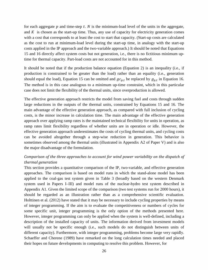
26

for each aggregate 𝑝 and time-step 𝑡. 𝑁 is the minimum-load level of the units in the aggregate, and 𝐾 is chosen as the start-up time. Thus, any use of capacity for electricity generation comes with a cost that corresponds to at least the cost to start that capacity. (Start-up costs are calculated as the cost to run at minimum-load level during the start-up time, in analogy with the start-up costs applied in the IP approach and the two-variable approach.) It should be noted that Equations 15 and 16 directly affect system costs but not generation, i.e., there is no fictitious minimum up-time for thermal capacity. Part-load costs are not accounted for in this method.

It should be noted that if the production balance equation (Equation 2) is an inequality (i.e., if production is constrained to be greater than the load) rather than an equality (i.e., generation should equal the load), Equation 15 can be omitted and 𝑔𝑐𝑝,𝑡 be replaced by 𝑔𝑝,𝑡 in Equation 16. The method is in this case analogous to a minimum up-time constraint, which in this particular case does not limit the flexibility of the thermal units, since overproduction is allowed.

The effective generation approach restricts the model from saving fuel and costs through sudden large reductions in the outputs of the thermal units, constrained by Equations 15 and 16. The main advantage of the effective generation approach, as compared with full inclusion of cycling costs, is the minor increase in calculation time. The main advantage of the effective generation approach over applying ramp rates is the maintained technical flexibility for units in operation, as ramp rates limit flexibility regardless of whether units are in operation or idle. However, the effective generation approach underestimates the costs of cycling thermal units, and cycling costs can be avoided altogether through a step-wise reduction in generation. This behavior is sometimes observed among the thermal units (illustrated in Appendix A2 of Paper V) and is also the major disadvantage of the formulation.

Comparison of the three approaches to account for wind power variability on the dispatch of thermal generation This section provides a quantitative comparison of the IP, two-variable, and effective generation approaches. The comparison is based on model runs in which the stand-alone model has been applied to the coal-gas test system given in Table 3 (broadly based on the western Denmark system used in Papers I–III) and model runs of the nuclear-hydro test system described in Appendix A1. Given the limited scope of the comparison (two test systems run for 2000 hours), it should be regarded as an illustration rather than as a comprehensive scientific evaluation. Holttinen et al. (2012) have stated that it may be necessary to include cycling properties by means of integer programming. If the aim is to evaluate the competitiveness or numbers of cycles for some specific unit, integer programming is the only option of the methods presented here. However, integer programming can only be applied when the system is well-defined, including a description of the installed capacity of units. The information derived from investment models will usually not be specific enough (i.e., such models do not distinguish between units of different capacity). Furthermore, with integer programming, problems become large very rapidly. Schaeffer and Cherene (1989) have remarked on the long calculation times needed and placed their hopes on future developments in computing to resolve this problem. However, for

27

Table 3. Composition of the coal-gas test system in terms of individual units (for the IP approach) and in terms of aggregates (for the two-variable and effective generation approaches).

performing calculations on a single stationary PC, integer programming remains confined to the evaluation of regions of limited geographic scope, such as western Denmark (as used in the present research). Since wind power integration is relevant not only for the regional electricity system, but also involves cooperation between electricity systems for electricity exchange, there are incentives to look for other methods.

An increase in wind power production in an electricity generation system where no active strategy for variation management is applied can be managed by; 1) part load operation in thermal units, 2) stopping electricity generation units or 3) curtailing wind power. Consequently, an increase in variations will be reflected as 1) an increase in start-up costs, 2) an increase in part load costs, 3) a shift from base load to peak load generation (in order to reduce start-up costs or

Max power [MWe]

Min power [% of max]

Run cost [€/MWh]

Fuel Start time [h]

Enstedverket_B3 660 35 % 33.4 coal 6

Fynsverket_B3 266 20 % 36.2 natural gas 6

Fynsverket_B7 374 35 % 33.4 coal 6

Nordjyllandsverket_B2 295 35 % 33.4 coal 6

Nordjyllandsverket_B3 411 35 % 33.4 coal 6

Skerbeverket_B3 392 20 % 36.2 natural gas 6

Studstrupverket_B3 350 35 % 33.4 coal 6

Studstrupverket_B4 350 35 % 33.4 coal 6

Esbjergverket_B3 377 35 % 33.4 coal 6

Herningeverket 89 20 % 36.2 natural gas 6

Peak 1000 0 44.1 natural gas 0

Gas steam 747 20 % 36.2 natural gas 6

Coal 2817 35 % 33.4 coal 6

Gas turbines 1000 0 44.1 natural gas 0

28

part load costs) or 4) an increased curtailment. The comparison of the three approaches to account for flexibility related properties of thermal generation is therefore based on an evaluation of the cycling costs, including start-up costs and part load costs, and the capacity factors of different generation technologies, which reflect a shift from base load to peak load generations and wind power curtailment. The total system costs reflect the economic impact of both cycling costs and capacity factors for different technologies and is the variable to be minimized in the optimization (Eq. 1). Table 4 gives the modeled productions for wind-power plants, gas turbines, and coal- and gas-fired steam power plants relative to the demand for electricity for the coal-gas test system when applying the three above-mentioned methods to model thermal generation. The three tables (Table 4a–c) represent three different levels of wind-power penetration (i.e., total possible wind power generation relative to the total load for the 2000 hours). The wind power penetration levels correspond to wind generation data derived from: 1) existing statistics for the present western Denmark system (26% wind penetration); 2) doubling the present wind generation (51% wind penetration); and 3) tripling the present wind generation (77% wind penetration)5 F

6. The results from model runs applying the three different methods to account for the costs of flexibility are compared to a reference case in which no cycling costs are included.

If cycling costs are not included, curtailment will only take place when wind-power generation exceeds the load. With the costs of cycling included (i.e., in the effective generation, two-variable, and IP approaches), the extent to which wind power is curtailed to avoid cycling costs obviously depends on the difference in running costs between wind power and thermal generation given by fuel prices and costs for emitting CO2. As indicated by the results presented in Table 4a–c, curtailment is slightly higher if cycling costs are fully accounted for, i.e. if either the IP approach or the two-variable approach is applied instead of applying the effective generation approach or if omitting cycling costs. If cycling costs are not accounted for, the load is met by wind-power generation and generation in coal-fired units, since the coal-fired units have lower running costs than gas-fired units (applying the costs of coal and gas assumed here). However, with cycling costs included, gas-fired generation is put into operation and the share of the load supplied by gas-fired generation increases as wind generation increases.

For the coal-gas test system, the two-variable approach provides estimates of the cycling costs, as well as the total system cost (cf. Table 4), which are well in line with the estimates provided by the IP approach. For this test system, the capacity factors of the gas turbines and the wind power are almost identical when applying the IP approach and the two-variable approach at all wind-penetration levels. However, assuming that the IP approach delivers solutions that most accurately reflect reality, the two-variable approach overestimates the capacity factor of coal capacity at the expense of gas steam capacity. In contrast, the effective generation approach generally overestimates the capacity factor of gas steam capacity, owing to the low-minimum

6 If wind power generation is doubled or tripled this would obviously affect the system configuration, i.e., some thermal generation would be terminated. The systems analyzed here do not represent credible future developments but merely test the methods.

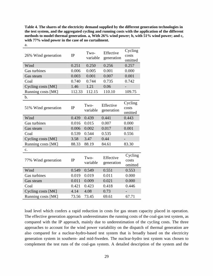
29

Table 4. The shares of the electricity demand supplied by the different generation technologies in the test system, and the aggregated cycling and running costs with the application of the different methods to model thermal generation. a, With 26% wind power; b, with 51% wind power; and c, with 77% wind power in the case of no curtailment. a.

26% Wind generation IP Two-variable

Effective generation

Cycling costs omitted

Wind 0.251 0.250 0.256 0.257 Gas turbines 0.006 0.005 0.001 0.000 Gas steam 0.003 0.001 0.007 0.001 Coal 0.740 0.744 0.735 0.742 Cycling costs [M€] 1.46 1.21 0.06 - Running costs [M€] 112.33 112.15 110.10 109.75 b.

51% Wind generation IP Two-variable

Effective generation

Cycling costs omitted

Wind 0.439 0.439 0.441 0.443 Gas turbines 0.016 0.015 0.007 0.000 Gas steam 0.006 0.002 0.017 0.001 Coal 0.539 0.544 0.535 0.556 Cycling costs [M€] 3.58 3.47 0.44 - Running costs [M€] 88.33 88.19 84.61 83.30 c.

77% Wind generation IP Two-variable

Effective generation

Cycling costs omitted

Wind 0.549 0.549 0.551 0.553 Gas turbines 0.019 0.019 0.011 0.000 Gas steam 0.011 0.009 0.021 0.000 Coal 0.421 0.423 0.418 0.446 Cycling costs [M€] 4.14 4.08 0.73 - Running costs [M€] 73.56 73.45 69.61 67.71

load level which confers a rapid reduction in costs for gas steam capacity placed in operation. The effective generation approach underestimates the running costs of the coal-gas test system, as compared with the IP approach, mainly due to underestimation of the cycling costs. The three approaches to account for the wind power variability on the dispatch of thermal generation are also compared for a nuclear-hydro-based test system that is broadly based on the electricity generation system in southern- and mid-Sweden. The nuclear-hydro test system was chosen to complement the test runs of the coal-gas system. A detailed description of the system and the

30

results from the model runs (corresponding to Tables 3 and 4) can be found in Appendix A1. The two-variable approach generally provides a good estimate of the running costs also for this system, while the effective generation approach generally underestimates the running costs. For the nuclear-hydro test system with 69 % wind power the running cost of the system is 16% lower if cycling costs are omitted compared to if the IP approach is applied. With the two-variable approach or the effective generation approach, running costs are only 1% or 3% lower than the running costs generated by the IP approach, respectively.

Figure 3 gives the resulting generation patterns of the units in the test system for 1 week in the summer with wind power penetration levels of 77% (i.e., about 55% after curtailment) for the different approaches to model cycling costs for the system defined in Table 3. In all the cases (a–d), wind power alone supplies the system with electricity for the first 2 days (Hours 1 to 47). The applied model was designed to compare the three different methods to account for cycling costs of thermal generation and does not include requirements for reserves that are available to respond to changes in frequency and cover for uncertainties or variations within the hour. Figure 3a shows the generation pattern for the case without any cost for thermal cycling. This results in that the coal-fired aggregate meets the peaks in thermal load even when the peaks are of short duration, while it reduces production to zero during other times (see, for example, Hour 85 in Figure 3a). However, the model demonstrates that this generation pattern is no longer optimal from a system cost perspective if cycling costs are taken into account. When the effective generation approach is applied (Figure 3b), the more extreme peaks (Hour 75) and troughs (Hour 85) in the generation levels in the coal power plants are removed. In this case, generation corresponding to 35% of the peak (the minimum-load level) in the modeling has to be paid for during a period of at least 6 hours, whereas the need for thermal generation is rapidly reduced after the peak. Rather than paying for thermal capacity that is not put in operation, some of the generation produced by coal-fired power plants is replaced by generation from gas-fired steam power plants (with a lower minimum-load level) and gas turbines (with no cycling costs in the model). Figure 3b shows a step-wise decrease in generation during hours 75 to 85 that is provoked by the modeling method itself rather than any physical constraints. Figure 3c gives the generation pattern of the test system when the two-variable approach is applied. With this method, the peaks in coal generation are flattened. The roof on generation in coal-fired power plants, as illustrated in Figure 3c, corresponds to the heated thermal capacity for which a start-up cost has been paid. The modeling avoids additional start-up costs by maintaining the minimum level of generation at 35% of this roof. The level of the heated capacity reflects a balance between curtailment during high-wind, low-load hours and gas turbine operation during low-wind, high-load hours. The generation in the coal-fired aggregate (Figure 3c) is similar to the aggregated generation of the coal -fired units modeled individually in Figure 3d, which illustrates what happens when the IP approach is applied. However, on an individual level, the IP approach gives very different generation patterns for different units within an aggregate due to differences in the sizes of the thermal units. Two of the coal-fired units are not taken into operation at all during the week depicted in Figure 3d.

31

Figure 3. Production patterns modeled for the system specified in Table 4, applying the stand-alone regional model of this work. Wind power alone supplies the system with electricity the first 2 days (Hours 1-47). a. Generation pattern without the costs associated with thermal cycling. b. Generation pattern when the effective generation strategy is applied. c. Generation pattern from the use of the two-variable approach. d. Generation pattern when the IP approach is used.

32

Figure 4. Marginal costs for electricity generation in the test system with 77 % wind power penetration as given by the model when applying the effective generation approach, the two-variable approach and when omitting cycling costs.

Figure 4 shows the marginal cost for generating electricity for the week illustrated in Figure 3a–c for the test system with 77% wind power, as given by the regional model applying the two-variable approach, the effective generation approach, and omitting cycling costs. The marginal costs for electricity generation given by the model applying the IP approach are without relevance, since a change in load may change fundamentally the dispatch. When cycling costs are omitted, the marginal cost is either the running cost of wind farms or the running cost of coal-fired power plants, as expected. With the effective generation approach, there are two peaks in marginal costs (Hours 79–81 and Hour 92), corresponding to electricity generation in gas turbines, which supply the peaks in net load prior to low-load events. There is an additional event with very low marginal costs (Hour 98), as compared with the case in which cycling costs are omitted. The low marginal costs in Hour 98, applying the effective generation approach, is due to the constraint of paying a running cost that corresponds at least to the start-up cost of the thermal capacity, despite a low net load. With the two-variable approach, marginal costs are low in Hours 94-99 due to the minimum-load level of the coal-fired aggregate, which exceeds the net load. During the two temporary reductions in marginal costs, in both the effective generation and two-variable strategies, the thermal generation in operation has running costs that exceed the marginal cost. The application of gas turbines to cover the peak load indicated in Figure 3c is reflected in the marginal costs of electricity generation in the two-variable case. Since start-up costs of gas turbines in the test system are omitted, there are no start-up costs reflected in the marginal costs for electricity with the two-variable approach.

The impact of including cycling costs has also been investigated on a European level. The electricity generation system analyzed in Paper V, in which 17% of the electricity demand is

33

supplied by variable renewables, was analyzed with the two-variable approach, the effective generation approach, and without accounting for cycling costs. It was found that the total system costs using the two-variable approach were 5.4% higher than when cycling costs were not accounted for in the model. The impacts of cycling costs on the fuel mix were concentrated to a few regions that typically have large amounts of nuclear power capacity installed (e.g., regions of France and Sweden) or high levels of wind power penetration (e.g. regions in the UK and Germany) or are connected to such regions. In these regions, the level of nuclear power generation was up to 16 TWh/year higher (corresponding to up to 23% more nuclear power supplying the regional demand for electricity) if cycling costs were excluded, as compared with a situation in which cycling costs were accounted for using the two-variable approach. With the two-variable approach, gas-fired generation mainly replaces nuclear power in the modeling. For the ten regions in which cycling costs have significant impacts, the effective generation approach generates capacity factors for the aggregates that lie intermediate to the capacity factors from the model applying the two-variable approach and the capacity factors from the model in which cycling costs are not included.

Shortt et al. (2013) have investigated the impact of accounting for variability by comparing results from a unit commitment dispatch model (similar to the IP approach in this thesis) and a dispatch-only model (similar to the cycling costs omitted approach in this thesis). They conclude that the impact of accounting for variability is highly system specific and that the presence of nuclear power increases the importance of accounting for variability due to its strong influence on start-up costs and dispatch order, which is in line with the findings of this thesis.

3.2.3 Time resolution and temporal scope Several approaches can be used to reduce the time dimension in models of the electricity generation system, so as to reduce model run times and computing requirements. One common approach, which is applied in ELIN, REEDS, and TIMES in Table 2, involves the subdividing of time into weighted load hours (i.e., workday peak load, workday low load, weekend etc.). However, for systems with high levels of wind power, defining representative hours is problematic. The number of combinations of availability of variable generation and load situations is infinite and thus, the problem of reducing the time dimension becomes a problem of accounting for a sufficient number of situations to generate a complete picture. If limitations regarding the flexibility of thermal units (i.e., start-ups) are to be included, there is also a need for consecutive time-steps, whereby an individual time-step is no longer than the start-up time. The step frequency also has to be sufficiently high to give a good representation of the load and wind-power variations (the frequency that is required here is dependent upon the research question posed). Increasing the time-steps from 1 hour to 3 hours is thus one of the few feasible ways to reduce the time dimension in models that are intended to investigate systems with high levels of wind power. Assuming that it would be sufficient to take one third of the time-steps into account, the optimization problem could be drastically reduced and computational times shortened (or other dimensions could be expanded). Another reason for evaluating the impact of applying a

34

lower time resolution is data availability. The European wind dataset applied in Papers IV–VI has a 3-hour time resolution. For this reason, a 3-hour time resolution has been applied in Papers V and VI. (Paper IV applies an hourly time resolution with linear interpolation between the 3-hour data-points. Papers I–III use a wind dataset with hourly time resolution and applies an hourly time resolution.)

Comparison: 1-hour and 3-hour time resolutions Table 5 compares model runs with time resolutions of 1 hour and 3 hours applied to the coal-gas test system described in the previous section, modeled for 2000 hours and 666 hours, respectively. The three methods to account for thermal cycling (described in the previous section) are applied to account for thermal cycling. The comparison is made at the highest wind penetration level of 77% prior to curtailment, since variations have greatest impact on the system at high levels of wind penetration. A comparison with a lower level of wind penetration, i.e., 26 %, which is more in line with the systems analyzed in Papers I–VI, is given in Appendix A2. As shown in Table 4, the impact on the total system cost of reducing the time resolution from 1 hour to 3 hours is ≤1% in all cases. Total system running costs are generally slightly underestimated when the lower time resolution is applied. Figure 5 illustrates the dispatch of the coal-gas test system at a 3-hour time resolution when applying the IP approach to model thermal cycling. The figure is more “coarse” in nature than Figure 3d, where hourly resolution has been applied. The need for gas turbines around Hour 75 cannot be identified with the 3-hour time resolution and a small amount of coal-fired generation is replaced with gas steam (Hours 100-140). Still, the dispatch in Figure 3d and Figure 5 is very similar. As given in Table 5, wind power curtailment and the capacity factor of coal are slightly underestimated with the 3h time resolution. However, in general, the impact of reducing the time resolution has little impact on the capacity factor.

Table 5. Shares of the electricity demand supplied by different generation technologies, as given by the stand-alone regional model and applying the three different methods to account for flexibility and a time resolution of 1 hour or 3 hours.

77% Wind generation IP 1h IP 3h Two-variable 1h

Two-variable 3h

Effective generation 1h

Effective generation 3h

Wind 0.549 0.551 0.549 0.551 0.551 0.553 Gas turbines 0.019 0.019 0.019 0.016 0.011 0.010 Gas steam 0.011 0.012 0.009 0.011 0.021 0.022 Coal 0.421 0.419 0.423 0.421 0.418 0.415 Cycling costs [M€] 4.14 4.12 4.08 4.16 0.73 0.78 Running costs [M€] 73.56 72.81 73.45 72.80 69.61 69.01

35

Figure 5. Cost-optimal dispatch of the test system for 1 week in summer, as given by the stand-alone regional model with the IP approach and with a 3-hour time resolution being applied. Wind power alone supplies the system with electricity on the first 2 days (Hours 1–47).

Thus, it can be concluded that for the coal-gas test system, it is possible to account for thermal cycling by applying the IP method, the two-variable method or the effective generation method at a 3-hour time resolution. For the analysis of this system, the choice between applying the two-variable approach or the effective generation approach has a greater impact on the results than the choice between the 1-hour and 3-hour time resolution. There are two characteristics of the coal-gas test system that may lessen the impact of reducing the time resolution from 1 hour to 3 hours for this particular system: 1) the start-up time of the units in the test system is 6 hours, which is evenly divisible by three; and 2) the wind-power data series from western Denmark represents wind power that is well-distributed geographically. Wind power that is concentrated within a smaller geographic area is likely to be subject to greater variability within each 3-hour period.

3.2.4 Variation management strategies When modeling the operation of an electricity generation system that is subject to wind-power variability, the inclusion of limits and the costs of variation management is of major concern. Section 3.2.2 describes methods to include the costs of cycling thermal units. Other parts of the electricity generation system are often mentioned as being more suitable for variation management than steam power plants, such as hydropower, DSM, and storage. Variation management through the use of hydropower is included in Papers IV–VI, and Paper II investigates storage as a form of variation management. DSM is addressed in general terms in Paper V, while Paper III evaluates DSM with respect to the charging of PHEVs. There follows a description of how these components, and their limits as to flexibility, have been included in the models applied in this thesis.

36

Hydropower Similar to wind power, hydropower relies on a resource that has varying levels of availability. Run-of-river hydropower can be modeled in the same way as wind power, with a varying upper limit on generation that depends on the resource availability and installed capacity. However, generation of hydropower with storage is not directly dependent upon the inflow. Nevertheless, resource constraint is also of high importance for hydropower with storage. The work within this thesis applies two common, basic ways of modeling hydropower with storage. In the first strategy, all hydropower is assumed to comprise two types: run-of-river hydropower; and hydropower with storage. The power ratings of the two types are taken from statistics on hydropower generation; therefore, this method will be referred to as the “statistical method”. When hydropower with storage is exposed to flooding in springtime, as happens in the Nordic countries, the fraction that cannot be stored due to storage limitations is taken as run-of-river hydropower in the statistical method. In contrast, hydropower generation that can be stored is only limited by the capacity and total yearly production. In the second strategy, using the “aggregated dynamics method”, hydropower stations within the same region, 𝑖, are aggregated, and storage is modeled with storage limitations and an equation that links the aggregated storage level 𝑙𝑖,𝑡 with the aggregated hydropower inflow 𝐻𝑖,𝑡and the regional hydropower generation, 𝑔ℎ𝑦𝑑𝑟𝑜,𝑖,𝑡 , as follows:

𝑙𝑖,𝑡++1 ≤ 𝑙𝑖,𝑡 + 𝐻𝑖,𝑡 − 𝑔ℎ𝑦𝑑𝑟𝑜,𝑖,𝑡 (17)6F

7

This aggregated dynamics method is, for example, applied in the BALMOREL model (Ravn, 2001b). The statistical method does not require ordered time-steps and can be acceptable for operational situations that resemble the present one, i.e., when modeling the present system or a near-term future system with no change that immediately affects hydropower scheduling. The aggregated dynamics method is an approximation of the actual limitations of flexibility of hydropower and can therefore be applied to future scenarios, although this requires ordered time-steps and information on storage limitations. However, the aggregated dynamics method disregards certain properties, such as per-station-defined reservoir limits (according to a water-rights court ruling) and the hydrologic coupling of two power stations on the same river. In Papers IV, V and VI, Nordic hydropower is modeled with the aggregated dynamics method, while the statistical method is applied to hydropower in the rest of Europe (Papers V and VI) owing to the lack of detailed data regarding hydropower outside the Nordic countries. The aggregated dynamics method was implemented in the EPOD model within the work of this thesis, to better account for the variation management that hydropower can provide. Figure 6 gives the total share of storage that is filled in the Nordic system, and compares weekly and

7 The expression ++ is a circular lag operator in GAMS. The term “++1” gives the subsequent member in the set, and if the current member is the last member of the set it gives the first member of the set. The hydropower storage level at the end of the year is thus required to be equal to the storage level at the beginning of the year: However, the determination of this level is part of the optimization process.

37

Figure 6. Hydropower reservoir levels in the Nordic countries, as obtained from the EPOD model (weekly and hourly model runs), as compared with the data from Nord Pool for Years 2011 and 2012 (Nord Pool, 2013).

hourly runs of the EPOD model to data obtained from Nord Pool. As shown in the figure, the aggregated storage levels given by model runs that apply the aggregated dynamics method follow the same trends as the real storage data for the Nordic system. Therefore, the aggregated dynamics method can be taken as a reasonable approximation of hydropower when assessing the general properties of electricity generation systems, such as marginal costs for generating electricity and trade patterns. However, owing to the simplifications made in the aggregated dynamics method, it cannot be considered an appropriate method for assessing the upper limits of hydropower as a balance resource or for answering other specific questions regarding hydropower.

When modeling parts of a year, as in Papers V and VI, the hydropower resource is distributed over the year in a model run with weekly time resolution. Inspired by the BALMOREL model (Ravn, 2001b), the results from the weekly model run fix storage levels in the first and last hour of the 3-week periods which are analyzed in greater detail. The hydropower generation within each 3-week period is optimized, with storage and capacity constraints taken in consideration. The distribution of the hydropower resource in the weekly model run is mainly based on the load and wind resource distribution over the year and the hydro inflow, with a large hydropower outtake during the high-load winter period.

Storage and Demand Side Management In an electricity generation system that is supplied exclusively by variable generation (i.e., run-of-river hydropower, solar power and/or wind power), either the generation or load will have to be shifted in time to meet the balance constraint (Equation 2). Generation can be shifted in time using a storage technology, typically in the form of pumped hydropower or compressed air energy storage, and the load can be shifted in time using a DSM strategy, such as flexible charging of PHEVs or through the use of flexible heating and cooling devices. In a system in which, in addition to variable generation, thermal generation is present, it depends on the running

38

costs and cycling costs of the thermal units whether investments in storage and/or DSM will reduce the total system costs. The benefits of introducing some DSM strategy or storage also depend on which variations occur in the system and the ability of the chosen strategy to manage different types of variations.

The size, duration, and frequency of the variations to be managed give indications as to the desired power rating and storage capacity of the storage technology. Different storage technologies have different costs associated with power rating and storage capacity. For DSM, the power rating and “storage capacity” that can be provided obviously depend on both the characteristics of the electricity consumption and how much it can be shifted in time; the electricity for space heating can only be delayed as long as the temperature in the building is above some given limit.

In Paper II, a variation moderator (i.e., storage, trade or DSM) was introduced to a regional wind-thermal system. The moderator was limited to shift generation within predefined periods of time, i.e., days and weeks. This approach was chosen because the objective was to evaluate a general system service without specifying the technology. However, the approach is mainly valid for cases for which the variation pattern is known, for example, if load variations dominate the net load variations or if the moderator is DSM with a diurnal usage pattern. Theoretically, the daily balanced moderator could, for example, be found to be of no use in a system with constant load and 24 hours of good wind conditions followed by 24 hours with no wind-power generation. In contrast, a storage technology with the same power rating and storage capacity, but without the day as a temporal restriction, would be able to shift a substantial amount of energy from one day to the next. In the same case, an electrical load without a diurnal usage pattern that could be shifted 24 hours could also be very helpful in matching load to generation.

In Paper V, which investigates the relationship between DSM and congestion, efforts were therefore taken to define a set of constraints that would capture the limits in flexibility while allowing flexibility with respect to the time periods of load shifting or storage. The final constraints, applied in Paper V, resemble the constraints applied to model the hydropower reservoirs, as described in Equation 17, although in the case of DSM, the “reservoir level” , is dynamic and depends on the size of the load during the hours concerned. The DSM constraints are given by:

, , , , . (18)

, ∑ , , (19)

, ∑ , , (20)

where is the total demand put on hold in region at time . In Paper V, has a positive value, which implies that load shifting is only possible through delaying demand. In Equations 18–20, is the delayed demand and is that part of the delayed demand that is supplied at

39

time 𝑡. The delayed demand, 𝑑𝑑, is limited to a certain share of the load in the hour investigated. In other words, it is assumed that the demand that can be delayed follows the same pattern as demand in general. The upper limit of the supplied demand, 𝑑𝑠, is given as a share of the highest level of demand of the day investigated, since demand that has been delayed at different time-steps can be supplied in the same hour, whereas the capacities of the appliances that supply the delayed demand are limited. In Paper V, there is just one aggregated DSM strategy and one relationship between supplied and delayed demand. In the model setup for Paper V, 𝑑ℎ is required to be a positive value, so demand cannot be supplied prior to the actual load hour. While this is a sensible approach with regards to a dishwasher or a washing machine, a heat pump may “over-supply” the heating system to some extent before the occurrence of a low-wind, high-load event (negative 𝑑ℎ). The setup described in Paper V should be considered as a first approach, and future work could use Equations 18–20 as a starting point for a more detailed description of DSM and to differentiate between DSM technologies by applying different relationships between supplied and delayed demand (e.g., allowing only positive or also negative 𝑑ℎ values or different limitations on 𝑑𝑑 and 𝑑𝑠). Such a detailed description could also give technology-specific delay times 𝐿.

Figure 7 gives the load for 1 week in UK1 (England) without delayed demand, with the possibility to delay 10 % of the demand for up to 6 hours, and with the possibility to delay 20% of the demand for up to 24 hours. As is shown in Figure 7, afternoon peaks in load are removed already with 10% 6-hour load shifting, whereas the load pattern is completely altered (to fit better to the generation system) with 20% 24-hour load shifting.

Figure 7. Load shifting for 1 week in early spring in UK1 (England). From the results in Paper V, as given by the EPOD model.

40

Charging of plug-in hybrid electric vehicles In Paper III, the charging of PHEVs provides variation management to various degrees depending on the charging strategy used. The most flexible charging strategy applied in Paper III is referred to as ‘S-FREE’. With the S-FREE charging strategy, the decision as to whether to charge parked vehicles is made by the dispatch model (taking an alternative cost for fuel into account). S-FREE in Paper III uses a modified version of the hydropower storage equation from BALMOREL to account for electricity storage in the PHEV fleet:

𝑝𝑠𝑖,𝑡++1 = 𝑝𝑠𝑖,𝑡 − 𝑝𝑑𝑐𝑖,𝑡 + 𝜂𝑖𝑝𝑐𝑖,𝑡 − 𝑝𝑑𝑖,𝑡 (21)

where 𝑝𝑠𝑖,𝑡is the aggregated storage level of the batteries, 𝑝𝑑𝑐𝑖,𝑡is the discharging of PHEVs to supply the electricity generation system, 𝑝𝑐𝑖,𝑡 is the charging of PHEVs with efficiency 𝜂𝑖 , and 𝑝𝑑𝑖,𝑡 is the discharging of batteries through driving the vehicle. Charging electric vehicles is associated with an economic benefit for the electricity generation system that corresponds to avoided fuel costs (i.e., the cost of the gasoline that the vehicles would otherwise have used), whereas discharging (vehicle-to-grid) is associated with a corresponding fuel cost (i.e., the cost of gasoline that the vehicles will have to use for driving when the electricity in the battery is delivered to the grid). The upper limit of storage, 𝑝𝑠𝑖,𝑡 , is the total capacity of the batteries in the PHEVs, and the upper limit of the discharge from driving, 𝑝𝑑𝑖,𝑡 , is the total energy consumed through driving during time 𝑡. The aggregation of PHEVs implied by this approach over-estimates the flexibility that the vehicles can deliver. For example, while some vehicles may be parked only during the night and other vehicles may be parked only during the day, with this aggregated approach, night-time charging can supply vehicles that are parked only during the day as long as the battery capacity of the vehicles parked during the night is respected. In Paper III, the similarities in commuting habits ensure that the error due to aggregation remains small. When analyzing the entire vehicle fleet, rather than just vehicles used for commuting, errors caused by aggregation may need to be re-evaluated.

3.2.5 Modeling electricity exchange A good description of the transmission system is of particular relevance when modeling systems with high levels of wind power for the following reasons: 1) the geographic allocation of wind power is different from that of thermal generation units and 2) variations in wind-power generation are reduced as the geographic scope increases. Since new wind power has other points of connection than the power plants which reduce their levels of operation during high-wind events or which are replaced by wind power on a permanent basis, bottlenecks may arise in previously uncongested parts of the grid. The latter point indicates that the description of the transmission system has an impact on the variations that need to be addressed by the modeled generation system. An analysis of the impact of wind -power variability on the cost-optimal dispatch of generation units will thus be affected by the description of the transmission system.

Models of the electricity generation system always relate in some way to the electricity transmission and distribution system. In its basic form, one simply assumes a transmission

41

system without congestion until some geographic border is reached (Papers I–III). The resulting regions, which are defined by the major transmission system bottlenecks, can then be connected to each other. The level of detail that is included for the transmission system in the model of the electricity generation system is defined by the sizes of the uncongested regions and the relationships between these regions. The following sections describe the regionalization of the European transmission system and the relationships between the regions, as applied in Papers V and VI.

Regionalization The regionalization of the European electricity generation system that is applied in Papers V and VI uses the existing transmission system as its starting point. Regions are separated from each other based on congestion in the transmission grid (both existing congestion and expected congestion in the near future). Thus, the regions can have any geographic area. The optimal choice of number of regions to include in a model involves a trade-off between accuracy and calculation time. Each additional region adds an additional generation-load balance equation (Equation 2) and a whole range of aggregates of generation units (these would otherwise have been incorporated into other aggregates).

In Papers V and VI, the regionalization is based on congestion in the high-voltage transmission grid (200 kV and 400 kV) only, thus disregarding congestion at the low-voltage and medium-voltage levels. This is a straightforward approximation with regards to the operation of large thermal generation units, which typically are connected to the high-voltage grid. However, wind power and solar power are often connected at lower-voltage levels and if peaks in wind power and solar power are systematically curtailed due to congestion in the distribution systems (it may simply be more economical from a system perspective to dimension the distribution system in this way), this approximation may introduce some errors.

Since the introduction of wind power may cause congestion in previously uncongested parts of the grid, a perfect model would revise the regionalization to facilitate analysis of a future system. However, as this is not straightforward, it is not applied in this work. Alternatively, regionalization could be carried out by taking expected congestion into account. Thus, in Papers V and VI, the regionalization was carried out assuming development of the transmission system according to the ENTSOE-E 10-year plans (ENTSO-E, 2010). In some cases, the 10-year plans were complemented by more detailed information from local transmission system operators (ensg, 2009; German TSO:s, 2009). Figure 8 shows the regionalization of Europe applied in Papers V and VI. Future congestion can also be assessed based on resource (wind, solar, and biomass power) and infrastructural (gas and CCS) evaluations.

42

Figure 8. The regionalization of Europe applied in Papers V and VI. The regions are here colored according to wind and solar penetration levels for the system investigated in Paper V.

The description of the regions in the model should include generation aggregates (i.e., electricity generation units that share the same main properties, such as fuel, technology, and efficiency) and a region-specific load. The regions applied in Papers V and VI, each consists of a set of NUTS II units7F

8. The use of NUTS II units to specify regions facilitates the assessment of regional load and generation. In the case of load, we used the gross domestic product given with NUTS II resolution by Eurostat (Eurostat, 2012a) to weight the national load to regional loads. In the case of generation, we used the geographic definitions of NUTS II for ArcGIS and the coordinates of generation units given in the Chalmers Power Plant database (Kjärstad and Johnsson, 2007) to link capacity to each region in ArcGIS. When future scenarios were analyzed, thermal generation was allocated to old sites (i.e., sites of decommissioned capacity) and motivated by existing infrastructure (i.e., gas pipelines and docks for coal) and contracts (environmental assessments etc.). 8 The NUTS (Nomenclature of Territorial Units for Statistics) classification is a hierarchical system for dividing up the economic territory of the EU defined by EUROSTAT for the collection, development, and harmonization of EU regional statistics, socio-economic analyses of the regions, and the framing of EU regional policies. Eurostat, 2012b. NUTS - Nomenclature of territorial units for statistics, http://epp.eurostat.ec.europa.eu/portal/page/portal/nuts_nomenclature/introduction.

43

Relationships between regions -electricity exchange Electricity exchange between two modeled regions is subject to some constraint. In its simplest form, the constraint is a thermal limit on capacity or, if available, the NTC8F

9 value. NTC values constrain electricity exchange in Paper IV. However, electricity exchange between two nodes in the transmission system also depends on the generation and load situations. In a three node system (nodes 1–3), with connections 1-2, 2-3, and 1-3, a given electricity exchange across 1-2 and 1-3 implies that the electricity exchange for 2-3 is a given. In linear models of the electricity generation system, this dynamics is governed by the constraint:

𝑃𝑖,𝑗,𝑡 = 1𝑋𝑖,𝑗

× �𝜃𝑖,𝑡 − 𝜃𝑗,𝑡�, (22)

where 𝑃𝑖,𝑗,𝑡is the power transferred from node i to node j in time t, 𝑋𝑖,𝑗is the reactance of the connection between node 𝑖 and 𝑗, and 𝜃𝑖,𝑡is the phase angle at node 𝑖 in time 𝑡. The power transfer is linked to generation and load by Equation 2, which states that the sum of the generation and imported electricity must equal the sum of the exported electricity and load. The link between Equations 2 and 22 is given by:

𝐸𝑖,𝑡𝑖𝑚𝑝 − 𝐸𝑖,𝑡

𝑒𝑥𝑝 = ∑ 𝑃𝑖,𝑗,𝑡∈𝐽,𝑗≠𝑖 (23)

where 𝐽 contains all the nodes connected to 𝑖. Thus, Equation 23 simply states that the power flow in and out of a region equals the import into the region and the export from the region.

𝑃𝑖,𝑗,𝑡 is normally assigned an upper limit that corresponds to the thermal upper limit on electricity exchange over the connection. For the regionalization performed in Paper V, the thermal upper limit of the connections was not known and 𝑃𝑖,𝑗,𝑡was constrained based on 𝑋𝑖,𝑗 (a detailed description of how this is done is given in Paper V).

The linearized load-flow constraints given by Equation 22 are referred to as the DC load-flow constraints. This is a widely used method and is described for example in the text book on power systems by Wood and Wollenberg (1996). The linear load flow constraint is a simplification of the non-linear optimal power flow constraints on active and reactive power, as given by:

𝑃𝑖,𝑗,𝑡 = �𝑉𝑖,𝑡��𝑉𝑗,𝑡� �𝐺𝑖,𝑗𝑐𝑜𝑠�𝜃𝑖,𝑡 − 𝜃𝑗,𝑡� + 𝐵𝑖,𝑗𝑠𝑖𝑛�𝜃𝑖,𝑡 − 𝜃𝑗,𝑡�� (24)

𝑄𝑖,𝑗,𝑡 = �𝑉𝑖,𝑡��𝑉𝑗,𝑡� �𝐺𝑖,𝑗𝑠𝑖𝑛�𝜃𝑖,𝑡 − 𝜃𝑗,𝑡� + 𝐵𝑖,𝑗𝑐𝑜𝑠�𝜃𝑖,𝑡 − 𝜃𝑗,𝑡�� (25)

where �𝑉𝑖,𝑡�is the voltage magnitude at node 𝑖, 𝐺𝑖,𝑗 and 𝐵𝑖,𝑗is are the real (conductance) and imaginary (susceptance) parts, respectively, of admittance 𝑌 on the connection between 𝑖 and 𝑗.

9 The Net Transfer Capacity (NTC) is an estimate of the possible power flow over an interconnection made by the TSO taking the n-1 security criterion into account. The NTC value depends on the generation and load situation. However, ENTSO-E publishes typical NTCs for interconnections per season.

44

The admittance is the inverse of the impedance, 𝑍, which consists of the resistance, 𝑅𝑖,𝑗, and the reactance, 𝑋𝑖,𝑗 .

To obtain the linear load-flow constraint (Eq. 22), the following approximations and assumptions are made:

1) Resistance on the connection is negligible, which means that 𝐺𝑖,𝑗 ≈ 0 and 𝐵𝑖,𝑗 ≈1𝑋𝑖,𝑗

;

2) There is a flat voltage profile, and all voltages are put to 1 p.u. (per unit); and 3) The phase angle differences are small, which means that 𝑐𝑜𝑠�𝜃𝑖,𝑡 − 𝜃𝑗,𝑡� ≈ 1 and

𝑠𝑖𝑛�𝜃𝑖,𝑡 − 𝜃𝑗,𝑡� ≈ �𝜃𝑖,𝑡 − 𝜃𝑗,𝑡�.

In Papers V and VI, where load-flow constraints are applied, Equation 22 is simply added as a boundary constraint. In this form, the load-flow constraint adds one variable per region and time-step (the phase angle) to the model. Since the total sum of power flows relative to one node can be expressed by the generation and load in the same node (Equations 2 and 23), it is possible to replace the phase angle in Equation 22 with a generation and load matrix. The elements in the matrix are combinations of generation and load at the nodes in the system, referred to as Power Transfer Distribution Factors (PTDFs), and are recalculated for each operational situation investigated. PDTFs have been used, for example, in the Trade Wind project (Van Hulle et al., 2009).

Impact of including load-flow relations on trade in a modeled Europe The papers included in this thesis use approximately the same approach with regards to regionalization, i.e., the regions in both BALMOREL and regional EPOD define regions based on major bottlenecks in the transmission grid. However, the papers apply different constraints on electricity exchanges between these regions. In Paper IV, electricity exchange is limited by NTC values, whereas load-flow relations are included in Papers V and VI by applying the DC load-flow approach. The inclusion of the DC load-flow constraints increases significantly the calculation times, and with limited computational resources these constraints may require restriction of the geographic or temporal scope. This section investigates whether the additional computational efforts are motivated when analyzing a regionalized Europe. The investigation is carried out by comparing trade flows in the European electricity generation system, as given by EPOD, while applying the DC load-flow approach (Equation 22) to trade flows given by EPOD when electricity exchange is limited by thermal constraints only (i.e., the capacity constraint available if the NTC value is not known). The modeling was performed for three 4-week periods (with a 3-hour time resolution, this entails 672 time-steps). The upper thermal limits on the connections were the same in the two cases.

The model results indicate that the load-flow constraints have a low impact (0.5%) on total system costs for the system investigated. The impact of load-flow constraints on exports from one region to another was also compared. With the regionalization applied in EPOD, there are 76

45

connections in the investigated system and thus, 152 export possibilities (i.e., one in each direction). Figure 9 shows the frequencies of differences in annual exports between the unconstrained and the constrained case. A positive value indicates that export through the connection is increased when load-flow constrains are omitted, while negative values indicate that export is decreased. As shown in the figure, the export levels are similar in most cases, although there are some outliers with significantly higher or lower yearly export levels as load-flow relations are included.

The results from the modeled example indicate that exports within Germany and around to neighboring countries are particularly affected by including load-flow constraints. Figure 10 illustrates levels of trade in the constrained and unconstrained cases for one of the internal German connections (export from DE2 to DE1). In the unconstrained case, exports reach the upper thermal limit on several occasions, whereas this level is never attained in the constrained case, i.e., dynamics resulting from the inclusion of Equation 22 to constrain the power flow at levels below the thermal limit.

Figure 9. Additional yearly exported electricity without flow constraints, relative to the constrained case (i.e., Equation 22 is included). Distributions across the connections included in the modeling are shown (total of 152 export possibilities).

46

Figure 10. Exported electricity between DE1 and DE2 with and without load flow relations.

It should be noted that the level of congestion in the present system is known and investments have been guided by this information. In contrast, for the analysis of scenarios for future systems, congestion levels will remain unknown as long as load-flow constraints are omitted. From an analysis of the present system, the above comparison thus gives a lower limit to the differences in trade between a constrained case and an unconstrained case (i.e., with or without Equation 22). When analyzing future electricity systems, the role of load-flow relations is not only to generate physically possible trade flows, but also to allow congestion to influence investment decisions.

The DC load-flow approach, which is used in the example above, as well as in Papers V and VI, includes relationships between regions in the same synchronous system, although it is still only an approximation of the full power-flow constraints (see Equations 24 and 25). Purchala et al. (2005) started from the approximations made in the DC load-flow approach and defined operational limits within which the method gives less than a 5% error. They found that the vast majority of networks that they tested had properties within these operational limits, but that there are systems for which the DC load-flow method gives errors that are >5% of the line flow. Thus, based on their research, it appears that the DC load-flow approach is a sufficiently good approximation, especially when considering modeling that is primarily directed towards energy policy issues and covering a wide geographic scope.

Duthaler et al. (2008) discussed the usability of the PTDF method (explained briefly above) for the UCTE network9F

10. They found that owing to the highly meshed network, small differences in the choice of zones could have large impacts on the PTDF matrix. They also found that internal

10 The UCTE (Union for the Co-ordination of Transmission of Electricity) network is the synchronous transmission system of continental Europe.

47

bottlenecks in the UCTE system were of great importance for the network analysis. The work conducted by Duthaler et al. (2008) confirms the need for regionalization beyond national borders, although it also indicates that, given the importance of the choice of regions, the regionalization may require revisions that reflect future invesments in tranmsisison and generation capacity.

Transmission limitations in future systems In Papers V and VI, the electricity generation system is modeled for Year 2020. With such a short time perspective, the transmission system can be approximated with the present system. (Planning and constructing a new transmission line is a time-consuming process, and there are lines that are currently in the planning phase that will first enter operation by Year 2020). A DC load-flow description of the transmission system for studies that have a longer time perspective is challenging due to the non-linear relationship between load-flow equations and transmission line investments. Investment models with thermal constraints or approximated NTC constraints on transmission can, and often do, include transmission investments and remain linear. However, investments in transmission in models with thermal- or NTC-constrained transmission indicate economic benefits from increased trade rather than propose grid upgrades, and it is uncertain as to whether trade across the new capacity can be realized physically.

If transmission investments and load-flow constraints are combined in the same model, the model becomes non-linear. To maintain linearity, a separate grid or dispatch model, which includes DC load-flow constraints on transmission, can evaluate whether it is physically possible to use the new investments that have been suggested by a linear investment model. The NTC-value for the connections obtained by the dispatch model, or the overload of lines in the grid model, can be fed back as information to the investment model, which then re-evaluates the investment decision. This iterative approach can be continued until the investment decision is stable. Fürsch et al. (2013) have applied such an iterative approach to optimize transmission investments.

3.2.6 The impact of the unpredictability of wind power on the dispatch The unpredictability of wind power (i.e., the uncertainty of the actual wind-power production at the time of decision making) is outside the scope of this thesis, and methods to account for unpredictability have not been included in the models. This section discusses the possible consequences of omitting the unpredictability of wind power. The unpredictability of wind power affects the electricity generation system in two different ways: 1) the unit commitment decision is made based on imperfect information; and 2) the magnitude of the forecast inaccuracy influences the size of the reserves. All the models applied in this thesis have perfect foresight. Papers I–III apply static first and second reserve requirements. In Papers IV–VI, the need for reserves is not part of the modeling.

On many electricity markets, the dispatch of units is based on forecasts made 24–36 hours prior to the production hour. Thus, the units are scheduled based on a wind power forecast with rather a high level of uncertainty, and the dispatch of units may not be optimal with regard to the actual

48

wind-power production. The influence of the time between planning and production on systems with wind power has been investigated by Holttinen (2005). The models used in this thesis focus on the physical limitations of conventional power plants to cooperate with wind power rather than the market aspects. Nonetheless, the problem of planning errors remains, since the start-up time for large-scale combustion units is several hours and the planning of the operation of the unit still has to be based on wind-power forecasts.

The consequences of decision making based on imperfect information have been evaluated in this thesis by implementing a rolling planning horizon on the regional western Denmark model, BALWIND (see Section 3.1.2 for details of the model), for 12 weeks evenly distributed over the year. The applied forecast method was persistence, i.e., the forecast is that wind-power generation will remain at the current level and forecasts are updated hourly. The results (not shown here) are compared to the outcomes of model runs in which forecasting errors are ignored (i.e., perfect foresight). It is found that the scheduling of large coal- and gas-fired units based on wind-power generation forecasts available 5 hours prior to the hour of production has little impact on total system costs, i.e., the forecasting errors imply an increase in total system costs of 1% compared to the perfect foresight situation. Scheduling thermal units based on wind-power forecasts provided by the persistence approach results in an increase in wind-power curtailment of about 4.5 GWh/week in the western Denmark system with 20% wind power (share of total demand in the case of no curtailment), as compared with a hypothetical situation with perfect forecasting. Wind power is curtailed to make way for coal-fired units, which are already scheduled to enter production, and the switch from wind to coal accounts for the vast majority of the increase in total system costs (fuel costs and the cost of CO2 emissions, here assumed to be 20 €/tonne). An increase in the number of start-ups of thermal units (with associated costs and emissions) is also noted.

The unpredictability of wind power results in a dynamic reserve allocation, whereby requirements for reserves are higher during time periods for which high-wind power generation is forecasted and lower during time periods for which low-wind power generation is forecasted (Kiviluoma et al., 2011). Depending on the flexibility of the generation units and their status (“hot capacity” or idle), they have different abilities to contribute to fulfilling the reserve constraints. Therefore, the capacity of the reserves required in the constraints can also have an impact on the decision to start generation capacity or to keep it idle.

The WILMAR model (Meibom et al., 2006) is designed to examine many possible scenarios, each of which is associated with different wind-power generation outcomes and associated reserve constraints. The scenarios are weighted according to the probability of the respective wind generation development and the total system cost of all the scenarios is minimized. Tuohy et al. (2009) investigated, using the stochastic rolling planning horizon approach of WILMAR, the consequences of making a decision regarding unit commitment based on perfect information on future wind and load situations, as compared to basing this decision on forecasts (“state-of-the-art” forecasts in Year 2009). They found that the total system costs were underestimated by

49

0.8%–1.5% depending on the forecast update frequency for the Irish system with 34% wind power. This can be compared to the 5% difference in total running costs for the western Denmark system with 24 % wind power if start-up costs are excluded (Paper I).

In summary, the uncertainty of wind power stimulates an increased need for reserves during high-wind events and a sub-optimal scheduling of thermal units. The uncertainty of wind-power generation can have an impact on the dispatch and cause wind-power curtailment and give higher capacity factors to inflexible base load units. The reasons for this are: 1) the forecasting applied for scheduling thermal units may underestimate or overestimate the wind generation, and in a case in which wind generation is underestimated, some thermal units are, sub-optimally, scheduled to start. Depending on the thermal units in operation and wind generation forecasts for the forthcoming hours, the start-up of additional thermal capacity may cause curtailment. In a situation in which the forecast underestimates wind generation, some thermal unit with shorter start-up times will be entered into operation in a subsequent time-step; and 2) units with start-up times in the range of hours can only provide reserves if the units are in operation, and if base-load units are in operation the running costs of these units are generally low compared to more flexible units. For systems with between 20% and 40% wind power, the impact of unpredictability on the dispatch is likely to be lower than the impact of variability. As markets are developed to be more suited to variable generation (e.g., though intra-day trading) and forecasting improves, the impact of unpredictability on the dispatch will be reduced.

4 Conclusions and Discussion Methods to analyze the impact of wind-power variability on the dispatch on both regional and European levels are provided. This section provides conclusions and discussions on the methods developed and evaluated to account for wind-power variability in dispatch models, as well as on the outcomes from dispatch modeling of systems with various variation management strategies. Below, the main findings of the research presented in Papers I–VI are summarized and discussed, including some results from the evaluation of the methods applied in the papers presented in this summarizing chapter.

4.1 The impact of wind power variability on the dispatch of thermal generation From the modeling work in Papers I, V and VI it can be concluded that the impact of wind power variability on regional dispatch increases with:

• an increase in wind power penetration level; • the fraction of generation capacity subject to small variations in running costs, whereby

the capacity with relatively low running costs has relatively high start-up costs or a high minimum-load level (e.g., as in Paper I, which applies units with the same technology and fuel but with different power rating);

• the fraction of generation capacity with high start-up costs and high minimum-load level but low running costs (e.g., systems with substantial amounts of nuclear power, as in Paper V and VI).

50

The interrelationships between cycling costs and these three factors can be understood by the following observations. Since variations in net load increase with the level of wind-power penetration, cycling costs are more relevant in systems with high levels of wind-power penetration. As variations in the system increase, low cycling costs represent an increasingly relevant competitive advantage. If the units with the lowest running costs do not have the lowest cycling costs in the system, greater variations in net load will change the relative competitiveness of the units. For systems in which the differences in cycling costs between the generation units are large but the differences in running costs are small, the impact on the capacity factors of the generation units will be evident already at low levels of wind-power penetration. For the coal-gas test system, which was used in Section 3.2.2 to compare different approaches to account for cycling costs, the gas steam power plants had only slightly better cycling properties than the coal power plants but they had higher fuel costs per unit of generated power. Thus, wind-penetration levels have to be very high if the model results are to indicate a substantial shift in utilization from coal to gas steam when increasing the wind penetration (c.f. Table 4). An increase in net load variations changes the relative competitiveness of units of the same type but with different power ratings. Large thermal units typically have relatively low running costs, whereas small units have relatively low start-up costs and low minimum-load levels. With the integer programming approach, which takes the unit power rating into account, cycling costs can have a strong impact on the operation of individual thermal units already at 20% wind-power penetration, as shown in Paper I. For regions with generation technologies that have high start-up costs and high minimum-load levels, such as nuclear power, curtailment is likely to be more cost efficient than starting and stopping these units. For these systems, significant curtailment can occur already at relatively low levels of wind-power penetration (as indicated by regions in Germany and France in the model runs for Europe, as in Papers V and VI). In systems that encompass capacity with good cycling properties and low running costs, such as hydropower with storage, this capacity will obviously maintain a high capacity factor, and the capacity factors will be accurately estimated even if cycling costs are disregarded.

In analyzing the European system for Year 2020 with 17% variable generation (the model setup used in Paper V), the inclusion of cycling costs was found to have a significant impact on the dispatch for 10/50 regions. With cycling costs, wind-power curtailment is significantly higher (i.e., at least 100 GWh/year) in Germany, Denmark, France, and Ireland, as compared with the results obtained when cycling costs were omitted. If the cycling costs are taken into account, the capacity factors of nuclear power in Germany and Scotland are significantly lower (by 4 TWh/year and 16 TWh/year, respectively) and the capacity factors of gas-fired generation capacity in England, Ireland, Poland, Italy, and Spain are significantly higher (i.e., by 1–10 TWh/year). In Germany, Denmark, Scotland, and Ireland, impacts on the dispatch are observed mainly due to high levels of wind penetration (i.e., up to 100 % on an annual basis). For France, an impact is observed due to the large share of nuclear power generation. It is necessary to include cycling costs in the modeling of all regions in the system to see the full impact of variations in the 10 regions mentioned above, since otherwise the variations could be exported to

51

neighboring regions. However, it is possible to draw relevant conclusions regarding the fuel mix in any of the other 40 regions without taking cycling costs into consideration.

An integer programming approach to cycling costs is necessary to assess the competitiveness and capacity factors of individual units. For information on an aggregate level, such as the relationships between base-load and peak-load generation, the comparison given in Section 3.2.2 indicates that the two-variable approach, which accounts for cycling costs for aggregates of units by distinguishing between heated capacity and actual generation, could provide a reasonable approximation.

4.2 Variation management Taking together, Papers II, III and V give that in a wind-thermal system in which wind power generation supply 20% of the demand for electricity on an annual basis, load shifting from daytime to nighttime provides efficient variation management, whereas such load shifting is inefficient in systems with 40% wind power.

Papers II, III, and V all include active variation management strategies, such as storage and DSM. Papers II and III evaluate the impact of general storage capacity and the charging of PHEVs on a regional wind-thermal system. For the wind-thermal system investigated in Papers II and III, in which wind power supplies 20% of the electricity demand, cycling costs due to wind variations are mainly caused by nighttime wind-power generation. This is the case because only units with poor cycling properties (but low running costs) are in operation during the night, whereas units with good cycling properties designed to meet variations in load are in operation during the day. Thus, by shifting the load to the nighttime (or by storing electricity to the daytime), competition between inflexible base-load generation and wind-power generation can be avoided and the cycling costs of the system are efficiently reduced. This result can be expected for any system that includes units in which low running costs come at the expense of cycling properties (i.e., units that either have low running costs and poor cycling properties or higher running costs and better cycling properties). DSM in the household sector offers an opportunity to reduce the competition between wind-power and base-load units. In the case of charging PHEVs, it has been found that if charging starts as the vehicle is parked in the evening, the PHEV load is likely to coincide with a high household load and costs related to variations (i.e., the sum of the part-load costs, cycling costs, curtailment costs, and costs due to fuel shifting) increase. However, if the charging is delayed to late at night and early in the morning the charging of PHEVs could reduce costs related to the variations. It should be noted that since the cycling costs for wind-thermal systems with ≤20% wind power are low, these costs are not likely to drive the development of DSM.

As the level of wind-power generation increases relative to the level of electricity demand the importance of the diurnal load variations for total variations in the system are reduced. Irregular wind variations influence system operation and high-wind events can last several days. Paper II shows how variation management of a wind-thermal system with 20% wind power can reduce

52

system emissions by reducing thermal cycling, while the level of emissions in a system with 40% wind power can be further reduced if curtailment can be avoided. However, the results shown in Paper II also propose that curtailment in the 40% wind system cannot be substantially reduced by storing electricity during nighttime for use in daytime or by shifting the load from daytime to nighttime. To achieve a substantial reduction in curtailment in the system with 40% wind power, there is a need for storage times in the range of several days.

Paper V shows that, in a Europe where wind and solar supply 17% of the annual demand for electricity, congestion is usually more severe during peak-load hours than during low-load hours. However, congestion can also be severe during the night in the case of interconnections between regions where a large proportion of demand in one of the connected regions is supplied by wind power. In Paper V, both the relatively low capacity of shiftable load in regions with a high share of wind relative to demand and the time constraint on load-shifting strategies (i.e., up to 20% of the load can be delayed up to 24 hours) strictly limit the ability to reduce wind-related congestion in the transmission system DSM in the form of load shifting is thus not an alternative to transmission investments if the regions involved are largely supplied by wind power. In contrast, peak-load congestion is efficiently reduced through load shifting.

4.3 The relationship between the Nordic electricity generation systems and the rest of Europe

The role of the Nordic electricity-generation system in a European context depends on the balance between investments in interconnector capacity and investments in Nordic generation capacity. It is concluded from this work that if investments are directed towards interconnections, the Nordic generation system manages production and demand variations in continental Europe. If investments are directed towards Nordic generation capacity, the Nordic generation system tends to become a base-load supplier of electricity whereby variations in production and demand are balanced domestically within the Nordic countries.

In Paper IV, which investigates cost-optimal allocation of wind power in northern Europe, the Nordic system is a bulk supplier of electricity to continental Europe, i.e., electricity is constantly exported without any significant variation. For the system investigated, Sweden and Norway are subject to large wind-power expansions. Trade between the Nordic system and continental Europe is almost all one-directional, and the support from the Nordic system to manage variations in continental Europe (seen in current trading patterns as night-time imports and daytime exports by the Nordic system relative to continental Europe) is lost. Paper VI investigates a scenario that includes investments in HVDC lines that stretch from Norway to the UK and Germany. The line from Norway to Denmark is reinforced and HVDC connections within the UK and Germany are put into operation. In Paper VI, Norway acts as re-distributor of power geographically and in time, and manages the load and wind variations in Germany, Denmark, the Netherlands, the UK, and Sweden.

53

Variation management with the hydropower-rich southern Norway region follows the simple principle that power imported from Europe supplies the Norwegian load during hours of low load and/or high winds, while Norway uses hydropower both to cover domestic electricity demand and electricity export during periods of peak load and/or low winds. For the Year 2020 scenario investigated in Paper VI, trade between Norway and the UK, Sweden, and the Netherlands is mainly governed by load variations, while trade between Norway and Germany and Denmark is governed to a large extent by wind power generation.

For the system investigated, with planned reinforcements between Norway and the rest of Europe up to Year 2020, the exchange capacity only provides a minor contribution to variation management for all regions, with the exception of Denmark. Nevertheless, the total capacity of the connections between south Norway and neighboring regions that host ≥20% wind power capacity is 6.4 GW, which can be compared to a local recurring minimum load in south Norway of around 6 GW. Therefore, there may be instances when Norway cannot harness all the low-cost electricity offered by the neighboring regions, and variations will be passed on from one trading partner with relatively low marginal costs via Norway to some other trading partner with relatively high marginal costs. If there is an increase in the exchange capacity between Norway and the rest of Europe, these situations will occur more frequently.

From the work carried out in Papers IV and VI, it can be concluded that, for the Nordic system, low investments in interconnector capacity relative to investments in wind-power and hydropower capacities will result in reduced marginal costs. Low marginal costs are attractive to electricity-intensive industries and the general public but are less attractive to the power industry. Large investments in transmission relative to investments in capacity for wind power and hydropower give marginal costs in the Nordic system that correspond to the marginal costs during low-load hours in the UK or south Germany. Thus, wholesale prices for electricity are higher in the Nordic market than in the case with large investments in capacity in the Nordic countries everything else being constant. This is an attractive scenario for the power industry and in particular for the power industry in Norway, which will be able to “buy low and sell high” due to the storability of hydropower.

5 Future work As wind power and solar power are the main options for sustainable electricity generation, they will be key technologies in future electricity generation systems. Which technologies should complement wind and solar power generation is less clear. Most of the previous work in the field of variation management has been dedicated to regional wind or solar power integration, applying one variation management strategy at a time. A key issue for future work is to find a balance between centralized (e.g., transmission investments and trade with hydropower-rich Nordic countries) and decentralized (e.g., regional storage and DSM) efforts to manage variations.

54

With the introduction of some improvements, the EPOD and ELIN models could be applied to identify a balanced variation management strategy. The communication between the investment model (ELIN) and the dispatch model (EPOD) would have to be improved, so that the capacity factors for transmission investments, as well as thermal generation could be returned to the investment model and investment decisions could be re-evaluated with this information until convergence. The modeling package would also need some specific improvements, such as boundary conditions on reserve requirements and an evaluation of the performance of the hydropower formulation in systems with a high willingness to pay for variation management.

6 References Barth, R., Brand, H., Meibom, P., Weber, C., 2006. A Stochastic Unit-commitment Model for the Evaluation of the Impacts of Integration of Large Amounts of Intermittent Wind Power, 9th International Conference on Probabilistic Methods Applied to Power Systems, KTH, Stockholm.

Duthaler, C., Emery, M., Andersson, G., Kurzidem, M., 2008. ANALYSIS OF THE USE OF PTDF IN THE UCTE TRANSMISSION GRID, EPFL.

ECMWF, 2010. ERA-Interim u- and v-components of horizontal wind, surface solar radiation downward, skin temperature, http://www.ecmwf.int/research/era/do/get/era-interim.

Energinet, 2013. www.energinet.dk.

ensg, 2009. Our electricity transmission network: a vision for 2020, in: group, t.e.n.s. (Ed.).

ENTSO-E, 2010. TEN-YEAR NETWORKDEVELOPMENT PLAN 2010-2020, in: EuropeanNetworkofTransmissionSystemOperatorsforElectricity (Ed.), Brussels.

Eurostat, 2012a. Gross domestic product (GDP) at current market prices by NUTS 2 regions, http://epp.eurostat.ec.europa.eu/portal/page/portal/region_cities/regional_statistics/data/database.

Eurostat, 2012b. NUTS - Nomenclature of territorial units for statistics, http://epp.eurostat.ec.europa.eu/portal/page/portal/nuts_nomenclature/introduction.

EWIS, 2010. European Wind Integration Study (EWIS), in: Winter, W. (Ed.). transpower stromubertragungs gmbh, Brussels.

Fürsch, M., Hagspiel, S., Jägemann, C., Nagl, S., Lindenberger, D., Tröster, E., 2013. The role of grid extensions in a cost-efficient transformation of the European electricity system until 2050. Appl Energ 104, 642-652.

German TSO:s, 2009. Übersicht über die installierte Kraftwerksleistung und die Leistungsflüsse in den Netzgebieten der deutschen Übertragungsnetzbetreiber (Regionenmodell Stromtransport 2009), in: Amprion, EnBW, Transpower, Vattenfall (Eds.).

GWEC, 2013. Global Wind Statistics.

Holttinen, H., 2005. Optimal electricity market for wind power. Energ Policy 33, 2052-2063.

Holttinen, H., 2008. Estimating the impacts of wind power on power systems - summary of IEA Wind collaboration. Environ Res Lett 3.

55

Holttinen, H., Meibom, P., Orths, A., Lange, B., O'Malley, M., Pierik, J., Ummels, B., Tande, J.O., Estanqueiro, A., Matos, M., Gomez, E., Soder, L., Strbac, G., Shakoor, A., Ricardo, J., Smith, J.C., van Hulle, F., Milligan, M., Ela, E., 2009. Design and operation of power systems with large amounts of wind power, IEA Wind task 25, Finland.

Holttinen, H., Meibom, P., Orths, A., Lange, B., O'Malley, M., Tande, J.O., Estanqueiro, A., Gomez, E., Soder, L., Strbac, G., Smith, J.C., van Hulle, F., 2011. Impacts of large amounts of wind power on design and operation of power systems, results of IEA collaboration. Wind Energy 14, 179-192.

Holttinen, H., O'Malley, M., Dillon, J., Flynn, D., Keane, A., Söder, L., 2013. Steps for a complete wind integration study, 46th Hawaii International conference on System Sciences, Hawaii.

Holttinen, H., O'Malley, M., Dillon, J., Flynn, D., Milligan, M., Söder, L., Orths, A., Abildgaard, H., Smith, J.C., Van Hulle, F., 2012. Recommendations for Wind Integration Studies, in: Betancourt, U., Ackermann, T. (Eds.), 11th international workshop on large-scale integration of wind power into power systems as well as on transmission networks for offshore wind power plants. Energynautics GmbH, Lisbon, Portugal, pp. 343-350.

Holttinen, H., Pedersen, J., 2003. The effect of large-scale wind power on thermal system operation, 4th International workshop on large-scale integration of wind power and transmission networks for offshore wind farms, Billund, Denmark.

IEA, 2012a. CO2 emissions from fuel combustion -highlights.

IEA, 2012b. Renewable Energy Outlook.

Jordan, G., Venkataraman, S., 2012. Analysis of Cycling Costs in Western Wind and Solar Integration Study, National Renewable Energy Laboratory

Kiviluoma, J., Holttinen, H., 2006. Impacts of wind power on energy balance of a hydro dominated power system, EWEC. EWEA, Athens.

Kiviluoma, J., O'Malley, M., Tuohy, A., Meibom, P., Milligan, M., Lange, B., Holttinen, H., Gibescu, M., 2011. Impact of Wind Power on the Unit Commitment, Operating Reserves, and Market Design. Ieee Pow Ener Soc Ge.

Kjärstad, J., Johnsson, F., 2007. The European power plant infrastructure - Presentation of the Chalmers energy infrastructure database with applications. Energ Policy 35, 3643-3664.

Kumar, N., Besuner, P., Lefton, S., Agan, D., Hilleman, D., 2012. Power Plant Cycling Costs. Intertek APTECH, Sunnyvale, California.

Lew, D., Brinkman, G., Kumar, N., Lefton, S., Jordan, G., Venkataraman, S., 2013. Finding flexibility: Cycling the conventional fleet. IEEE Power and Energy Magazine 11, 20-32.

Loulou, R., Goldstein, G., Noble, K., 2004. Documentation for the MARKAL Family of Models. ETSAP.

Loulou, R., Remne, U., Kanudia, A., Lehtila, A., Goldstein, G., 2005. Documentation for the TIMES Model - PART I 1–78.

Mc Garrigle, E.V., Deane, J.P., Leahy, P.G., 2013. How much wind energy will be curtailed on the 2020 Irish power system? Renew Energ 55, 544-553.

56

Meibom, P., Barth, R., Hasche, B., Brand, H., Weber, C., O'Malley, M., 2011. Stochastic Optimization Model to Study the Operational Impacts of High Wind Penetrations in Ireland. Ieee T Power Syst 26, 1367-1379.

Meibom, P., Barth, R., Norheim, I., Ravn, H., Sørensen, P., 2006. Wind power integration in a liberalised electricity market (WILMAR), Risᴓ National Laboratory

National Renewable Energy Laboratory, 2010. Western wind and solar integration study, GE Energy, Colorado.

Nord Pool, 2013. Reservoir Content for Electrical Exchange Area.

Odenberger, M., Unger, T., Johnsson, F., 2009. Pathways for the North European electricity supply. Energ Policy 37, 1660-1677.

Power World, 2014. Power World, www.powerworld.com.

Purchala, K., Meeus, L., Van Dommelen, D., Belmans, R., 2005. Usefulness of DC power flow for active power flow analysis, Power Engineering Society General Meeting, 2005. IEEE, pp. 454-459.

Ravn, H., 2001a. Balmorel -Energy system model.www.eabalmorel.dk

Ravn, H., 2001b. Balmorel: A Model for Analyses of the Electricity and CHP Markets in the Baltic Sea Region.

Ritchers, J., 2011. DIMENSION – A Dispatch and Investment Model for European Electricity Markets. Institute of Energy Economics at the University of Cologne (EWI).

Saravanan, B., Das, S., Sikri, S., Kothari, D.P., 2013. A solution to the unit commitment problem -a reveiw. Front Energy 7, 223-236.

Schaeffer, P., Cherene, L., 1989. The inclusion of “spinning reserves” in investment and simulation models for electricity generation. European Journal of Operational Research 42, 178-189.

Short, W., Sullivan, P., Mai, T., Mowers, M., Uriarte, C., Blair, N., Heimiller, D., Martinez, A., 2011. Regional Energy Deployment System (ReEDS). National Renewable Energy Laboratory.

Shortt, A., Kiviluoma, J., O'Malley, M., 2013. Accomodating variability in generation planning. Ieee T Power Syst 28, 158-168.

Spiecker, S., Weber, C., 2014. The future of the european electricity system and the impact of fluctuating renewable energy - A scenario analysis. Energ Policy 65, 185-197.

Söder, L., Holttinen, H., 2008. On methodology for modelling wind power impact on power systems. International Journal on Global Energy Issues 29, 181-197.

Tuohy, A., Meibom, P., Denny, E., O'Malley, M., 2009. Unit Commitment for Systems With Significant Wind Penetration. Ieee T Power Syst 24, 592-601.

Ummels, B.C., Gibescu, M., Pelgrum, E., Kling, W.L., Brand, A.J., 2007. Impacts of wind power on thermal generation unit commitment and dispatch. IEEE Transactions on Energy Conversion 22, 44-51.

57

Unger, T., Odenberger, M., 2011. Dispatch modelling of the European electricity supply: the EPOD model, in: Johnsson, F. (Ed.), Methods and Models used in the project Pathways to Sustainable European Energy Systems, Mölndal, pp. 97-101.

Van Hulle, F., Tande, J.O., Uhlen, K., Warland, L., Korpås, M., Meibom, P., Sørensen, P.E., Morthorst, P.E., Cutululis, N.A., Giebel, G., 2009. Integrating wind: Developing Europe's power market for the large-scale integration of wind power. European Wind Energy Association.

Weber, C., 2005. Uncertainty in the electric power industry: methods and models for decision support. Springer.

Wood, A.J., Wollenberg, B.F., 1996. Power generation, operation and control. John Wiley & Sons.

58

Appendix A1. Comparison of the three approaches to account for wind power variability on the dispatch thermal generation in the nuclear-hydro test system

Table A1.1 Composition of the nuclear-hydro test system in terms of individual units (for the IP approach) and in terms of aggregates (for the two-variable and effective generation approaches).

Max power [MW]

Min power [% of max]

Run cost [EUR/MWh] Fuel Start

time [h]

O1 473 80% 24.6 nuclear 24

O2 638 80% 24.6 nuclear 24

O3 1400 80% 24.6 nuclear 24

R1 859 80% 24.6 nuclear 24

R2 866 80% 24.6 nuclear 24

R3 1045 80% 24.6 nuclear 24

R4 950 80% 24.6 nuclear 24

F1 987 80% 24.6 nuclear 24

F2 1120 80% 24.6 nuclear 24

F3 1170 80% 24.6 nuclear 24

hydro 7300 0 1 hydro 0

peak 1000 0 44.1 natural gas 0

nuclear 9508 80% 24.6 nuclear 24

hydro 7300 0 1 hydro 0

peak 1000 0 44.1 natural gas 0

59

Table A1.2 The shares of the electricity demand supplied by the different generation technologies in the test system, and the aggregated cycling and running costs with the application of the different methods to model thermal generation. a, With 26% wind power; b, with 51% wind power; and c, with 77% wind power in the case of no curtailment.

23% Wind generation IP two-variable

effective generation

cycling costs omitted

Wind 0.228 0.228 0.231 0.234 Gas turbines 0.001 0.001 0.000 0.000 Hydro 0.285 0.284 0.285 0.284 Nuclear 0.486 0.487 0.483 0.482 Cycling costs [MEUR] 1.03 1.15 0.00 - Running costs [MEUR] 290.64 291.30 287.44 286.39

46% Wind generation IP two-variable

effective generation

cycling costs omitted

Wind 0.419 0.419 0.419 0.427 Gas turbines 0.003 0.003 0.003 0.000 Hydro 0.285 0.284 0.285 0.282 Nuclear 0.293 0.293 0.293 0.292 Cycling costs [MEUR] 15.31 15.50 9.05 - Running costs [MEUR] 201.89 202.18 195.02 182.42

69% Wind generation IP two-variable

effective generation

cycling costs omitted

Wind 0.536 0.536 0.534 0.541 Gas turbines 0.003 0.004 0.004 0.000 Hydro 0.285 0.282 0.281 0.284 Nuclear 0.176 0.178 0.181 0.175 Cycling costs [MEUR] 19.05 19.36 12.21 - Running costs [MEUR] 141.61 143.35 138.05 118.56

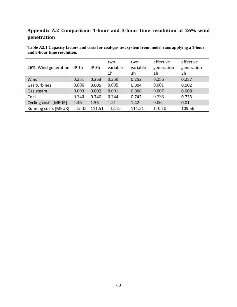
60

Appendix A.2 Comparison: 1-hour and 3-hour time resolution at 26% wind penetration

Table A2.1 Capacity factors and costs for coal-gas test system from model runs applying a 1-hour and 3-hour time resolution.

26% Wind generation IP 1h IP 3h two-variable 1h

two-variable 3h

effective generation 1h

effective generation 3h

Wind 0.251 0.253 0.250 0.253 0.256 0.257 Gas turbines 0.006 0.005 0.005 0.004 0.001 0.002 Gas steam 0.003 0.002 0.001 0.006 0.007 0.008 Coal 0.740 0.740 0.744 0.742 0.735 0.733 Cycling costs [MEUR] 1.46 1.53 1.21 1.42 0.06 0.01 Running costs [MEUR] 112.33 111.51 112.15 111.51 110.10 109.56