The Impact of the Manufacturer-hired Sales Agent

on a Supply Chain with Information Asymmetry

Neda Ebrahim Khanjari

University of Illinois

neda.khanjari@gmail.com

Seyed Iravani

Northwestern University

s-iravani@northwestern.edu

Hyoduk Shin∗

University of California - San Diego

hdshin@ucsd.edu

May 20, 2013

Abstract

This paper studies the impact of a manufacturer-hired sales agent on a supply chain

comprising a manufacturer and a retailer. The sales agent is working mainly at the re-

tailer’s location in order to boost the demand. We focus on a wholesale price contract,

under which the retailer decides how much to order from the manufacturer. The infor-

mation structure within the supply chain and the efficiency of the sales agent affect the

supply chain members’ expected profits. We show that, due to the agency issue between

the sales agent and the manufacturer, when the retailer’s demand forecast accuracy is

similar to the manufacturer’s and the wholesale price is fixed, the retailer’s profit is

decreasing in his demand forecast accuracy. We also illustrate that when the retailer’s

forecast accuracy is much better than the manufacturer’s and the wholesale price is

endogenous, his expected profit is decreasing in his forecast accuracy. Moreover, we

demonstrate that having a more efficient sales agent is beneficial for the retailer when

the wholesale price is fixed, whereas it is not always the case when the wholesale price

is determined depending on the efficiency of the sales agent.

∗The authors thank Steve Graves, the anonymous Associate Editor and the three anonymous referees for theirdetailed and extremely helpful comments and suggestions. They also thank Mark Daskin and Terry August forvaluable comments and discussions.

1 Introduction

Upstream manufacturers often sell their products to consumers through downstream retailers.

Many factors influence this relationship between a manufacturer and a retailer in a supply chain.

One such factor is a sales agent as an independent entity that can substantially alter the dynamics

within the supply chain. Sales agents are widely employed in the industry. According to Zoltners

et al. (2001), nearly twelve percent of the total workforce in the US is employed in full-time sales

occupations. Furthermore, firms’ average expenditure on salesforce typically ranges between ten

percent to forty percent of their sales revenues (Albers and Mantrala 2008). In addition, enhanced

salesforce management often can increase sales revenue by more than ten percent (Zoltners et al.

2008).

There are different types of sales agents depending on who hires them within a supply chain.

In this paper, we focus on sales agents hired by upstream manufacturers. U.S. Department of

Labor (2012b) has estimated that wholesale and manufacturing sales representatives held about

two million jobs in the U.S. in 2010. Specifically, in the automobile industry, sales agents are often

hired by auto manufacturers to boost demand at the dealer site. For example, these sales agents

are called area sales managers in Toyota. Based on the job description of these sales agents in

Toyota Financial Services (2012) and U.S. Department of Labor (2012a), the manufacturer-hired

sales agents increase demand by improving sales techniques of the retailer and/or marketing. In

this paper, we focus on the impact of a manufacturer-hired sales agent on the supply chain, in

which the primary task of the sales agent is to boost demand.

We focus on two influential factors: (i) the sales agent’s efficiency and (ii) the accuracy of the

available demand information at the downstream level. The first factor is how efficient the sales

agents are in fostering demand. A more efficient sales agent can increase demand by the same

amount as the less efficient one but using a smaller amount of effort. The second factor is the

degree to which information about local demand available at the downstream level (e.g., at the

retailer site) and not available to the manufacturer. Our primary research question is how the

expected profits of the manufacturer and the retailer depend on these two factors. For example, do

the manufacturer and the retailer always benefit from a more efficient sales agent or more informed

downstream parties?

1

To answer this research question, we examine a supply chain in which a manufacturer employs

a wholesale price contract with a retailer for a single product and hires a sales agent to boost

consumer demand. In this paper, we study both a fixed wholesale price model, and an endogenous

wholesale price model in which the manufacturer sets the wholesale price optimally.

We first characterize the optimal linear compensation contract for the manufacturer-hired sales

agent, and then demonstrate that even though more accurate demand information at the down-

stream level has a direct benefit to the supply chain, it can sometimes hurt the manufacturer, the

retailer, or both due to strategic interaction between the manufacturer and the sales agent. Fur-

thermore, we show that the impact of demand forecast accuracy at the downstream level on the

retailer’s expected profit depends critically on whether the wholesale price is fixed or set endoge-

nously. In addition, we illustrate that the retailer benefits from a more efficient sales agent if the

wholesale price is fixed. However, under an endogenous wholesale price model, the retailer may be

hurt by a more efficient sales agent.

This paper proceeds as follows: In Section 2, we review the related literature. We then present

the model in Section 3. We analyze the model with exogenous wholesale price, and endogenous

wholesale price in Sections 4 and 5, respectively. Furthermore, we discuss extensions of our paper

in Section 6. Finally, we provide our concluding remarks in Section 7.

2 Literature Review

Our paper explores the impact of a sales agent on operational decisions within a supply chain.

One of the important problems related to a sales agent is how to structure the compensation

scheme, which has been studied in marketing and economics literature. Coughlan (1993) provides

a comprehensive review of salesforce management and compensation. For the compensation of

the sales agent, we consider a menu of linear contracts and focus on the impact of sales agent

contracting on the firm’s operational decisions, i.e., production and inventory choices, which has

been underexplored in the literature of marketing and economics.

The operations literature related to sales agents has studied the impact of sales agent com-

pensation on a firm’s operational decisions, e.g., inventory planning. Chen (2000) proposes a sales

agent compensation package to induce the agent to exert an effort in a way that smooths out con-

2

sumer demand across time. In practice, in particular at IBM, the compensation scheme proposed

by Gonik (1978) has been implemented. This scheme intends to provide incentives to the agent to

truthfully reveal what it knows about demand, based on the premise that the sales agent has more

accurate demand information, and to work hard also. Studying Gonik’s scheme and comparing it

with a menu of contracts, Chen (2005) shows that Gonik’s solution can be dominated by a menu of

linear contracts when the firm also determines the inventory level. Analyzing sales agent contract-

ing when demand information is censored by the inventory level, Chu and Lai (2012) demonstrate

that the optimal contract with the agent takes the form of a sales-quota based bonus contract, and

the optimal service level under this contract is always higher than the first-best level.

The new angle that we take in this paper is to understand the impact of a manufacturer-hired

sales agent on a supply chain, whereas the previous literature has focused mostly on the impact to

a single member of a supply chain (either a manufacturer or a retailer). One exception is Chen and

Xiao (2012), who study the impact of the retailer’s forecasting accuracy on both the manufacturer

and the retailer in the presence of a sales agent. They focus on a retailer-hired sales agent without

inventory consideration, whereas we analyze a manufacturer-hired sales agent with consideration

of the retailer’s inventory decision.

Among the few works that study the impact of a manufacturer-hired sales agent on the supply

chain, Hopp et al. (2010) is the most relevant paper to this study. They consider a supply chain

with a manufacturer-hired sales agent in a setting in which demand is deterministic. We also study

the impact of a manufacturer-hired sales agent, which corresponds to their wholesale-salesperson,

but under stochastic demand. Considering the demand uncertainties and information asymmetry,

we can then answer our research question, which cannot be answered using the prior model in

Hopp et al. (2010); we specifically develop a model to investigate how the impact of the sales agent

depends on the forecast accuracy of uncertain demand.

3 The Model

We consider a supply chain in which a manufacturer (she) employs a wholesale price contract with

a retailer (he), and she hires a sales agent (it) to boost demand. In Section 4, we study the fixed

wholesale price case (e.g., because of a prior long term contract between the manufacturer and

3

the retailer, or due to competition among potential manufacturers). In Section 5, we extend the

model to allow the manufacturer to set the wholesale price optimally. We restrict attention to

a wholesale price contract between the manufacturer and the retailer, which is common and the

simplest contract form employed between firms.

3.1 Demand and Information Structure

Consumer demand is random and depends on the market condition Θ, and the effort e that the

sales agent makes; specifically, consumer demand D is given as D = Θ+e, where market condition

Θ is normally distributed with mean θ and variance σ2 (or, accuracy h ≡ 1σ2), i.e., Θ ∼ N(θ, σ2).

Furthermore, the sales effort e can be interpreted as the amount of work that a sales agent needs

to exert to increase demand by e units.

At the retail site, information about regional demand is available due to the direct contact

with consumers and the potential availability of past sales data (see, e.g., Lee et al. 2000). Since

this information is often not available upstream, the retailer as well as the sales agent, who works

closely with the retailer to boost demand at the retail site, have an informational advantage about

regional demand compared to the manufacturer. For example, according to the job description of

the sales agent in Toyota, sales agents spend 75% of their work hours at the dealer site (Toyota

Financial Services 2012). Consequently, the retailer’s demand forecast is likely to be shared with

the sales agent. To model this informational advantage, we assume that the sales agent and the

retailer observe a private signal of demand, Ψ, that the manufacturer cannot obtain; specifically,

the retailer and the sales agent observe a noisy signal that is normally distributed with a mean

equal to the market condition, i.e., Ψ|(Θ = θ̂) ∼ N(θ̂, σ̃2). We define the accuracy of this signal for

the downstream parties as h̃ ≡ 1σ̃2.1 Lastly, all parameter values and the information structure are

common knowledge, and ψ is the only private information in our model.

3.2 The Sales Agent’s Cost and Payoff

We assume an increasing and convex cost function for the sales agent’s effort, reflecting the increas-

ing marginal cost of effort; specifically, the cost of effort is C(e) = 12ke

2, with k > 0 (see, e.g., Chen

and Xiao 2012). Note that k can be interpreted as the efficiency, or the competency, of the sales

1We acknowledge that our model and the results are limited to the normal distribution for signals.

4

agent. If k is higher, the sales agent can boost demand at a lower cost. Without loss of generality,

we normalize the sales agent’s reservation payoff to zero.

The effort of the sales agent includes improving sales techniques of the retailer by providing

him (i) more detailed product information, and (ii) marketing recommendations such as how to

lay out advertising materials within the retail location (Toyota Financial Services 2012). Note that

the sales agent’s effort directly involves or requires permission of the retailer. As a result, this effort

becomes observable by the retailer.2

For the compensation scheme of the sales agent, we focus on the form of a linear commission

in the observed outcome combined with a constant salary. This form of payment is (i) widely used

in practice (U.S. Department of Labor 2012b) as well as in research (see, e.g., Chen 2005) for sales

agent compensation schemes, (ii) easy to implement, and (iii) an optimal contract form in a broad

range of circumstances, as McAfee and McMillan (1987) have shown.

We consider the sales agent’s compensation to be contingent on the manufacturer’s demand (i.e.,

on the order quantity of the retailer). Note that the sales agent’s effort is usually not contractible,

which precludes the manufacturer from making the sales agent’s compensation directly contingent

on the effort.3 Specifically, in this paper, a sales agent’s compensation can be written as P (q) =

αq + β, where q is the retailer’s order quantity; α is the commission rate, and β is the constant

salary. Moreover, the manufacturer may offer a menu of linear contracts, {Pψ(q) = αψq+βψ : ∀ψ},

which will be self-selected by the sales agent, where ψ is the realization of the noisy signal Ψ. One

way to implement a menu of contracts is to employ a nonlinear compensation scheme, which has

been observed in practice (see, e.g., Oyer 2000). Furthermore, the sales agent has the option not

to engage in a contract.

3.3 The Retailer’s and the Manufacturer’s Profit Functions

We consider a single-period problem in which the manufacturer produces each unit of product at

a constant unit-production cost c, and sells it to the retailer at a wholesale price w. The product

is sold in the consumer market at retail price p and has zero salvage value. The insights in the

2However, in Section A.2 of the online supplement, we provide formal analysis of the case in which the effort ofthe sales agent is not observable by the retailer. We show that, in such a case, the sales agent does not exert anyeffort, and hence it does not have any impact on the supply chain.

3This assumption is also consistent with the field study of Hopp et al. (2010).

5

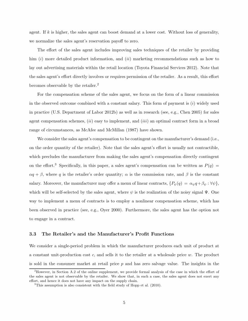
Downstreamparties observea market signal

Manufacturer (sets awholesale price and)offers contracts tosales agent

Sales agent choosesa contract andmakes an effort

Retailerdeterminesorder quantity

Demand isrealized

Figure 1: The sequence of events.

paper are preserved under a positive salvage value as long as it is less than the wholesale price. We

assume p > w > c > 0.

The retailer’s profit under order quantity q and realized demand x is ΠR = p min{x, q}−w q =

(p − w) q − p (q − x)+, where y+ ≡ max{y, 0}. Similarly, the manufacturer’s profit can be written

as ΠM = (w− c) q−Pψ(q), where Pψ(q) is the compensation to the sales agent when she observes

signal ψ and the retailer orders q. We refer to the sum of the retailer’s and the manufacturer’s

profits as the supply chain’s profit.

3.4 Sequence of Events

As illustrated in Figure 1, at the beginning, the downstream parties, i.e., the retailer and the

sales agent, observe a signal Ψ of the market condition and update their belief about the market

condition Θ. Then, the manufacturer offers a menu of linear contracts to the sales agent (and a

wholesale price contract to the retailer under endogenous wholesale pricing in Section 5). The sales

agent subsequently chooses a contract from the menu or rejects participating. Next, the sales agent

makes an effort to increase consumer demand. After observing the sales agent’s effort, the retailer

submits his order quantity to the manufacturer.4 The manufacturer then compensates the sales

agent and delivers the order quantity to the retailer, and lastly demand is realized.

4 Exogenous Wholesale Price

In this section, we focus on the case in which it is very costly for the manufacturer to change the

terms of her contract with the retailer; that is, we assume that the wholesale price is fixed at w.

We relax this assumption in Section 5 and explore the case in which the wholesale price is set by

the manufacturer.

4In Section 6, we discuss the case in which the sales agent makes an effort after the retailer places his order to themanufacturer.

6

4.1 Equilibrium Analysis

We use backward induction to obtain the equilibrium. First, we analyze the retailer’s problem of

his optimal order quantity. Note that since the retailer and the sales agent observe a signal of

the market condition, their belief about the market condition is updated according to Bayes rule.

Specifically, from the retailer’s and the sales agent’s perspective, given their observed signal ψ, the

market condition is Θ|(Ψ = ψ) ∼ N(hθ+h̃ψh+h̃

, 1

h+h̃).

The retailer observes the effort of the sales agent e. Therefore, the retailer’s expected profit

can be written as:

E[ΠR(q)] = (p− w)q − p

∫ q

−∞Φ

y − e− hθ+h̃ψ

h+h̃1√h+h̃

dy ,

where Φ(·) is the CDF of the standard normal distribution. The retailer’s objective function is

concave in q; thus, from the first order condition, we obtain the retailer’s optimal order quantity

as q∗(ψ, e) = q0 + e+ hθ+h̃ψ

h+h̃, where q0 satisfies Φ

(q0√h+ h̃

)= p−w

p .

Next, given the retailer’s optimal order quantity and the compensation scheme (α, β), we then

derive the sales agent’s optimal effort level e∗. The sales agent’s net payoff when exerting effort e

is

πs(e, α, β|Ψ = ψ) = α(q0 + e+

hθ + h̃ψ

h+ h̃

)+ β − 1

2ke2 . (1)

This is a concave function of e; consequently, the sales agent’s optimal effort is e∗(α) = k α.

Finally, we study the manufacturer’s problem of designing an optimal menu of linear contracts

to offer to the sales agent. Let (αψ, βψ) be the designated contract from the menu for the sales agent

who observes Ψ = ψ as a signal of the market condition. Then, we can write the manufacturer’s

problem as follows:

maxαψ≥0, βψ

Eψ

[(w − c− αψ

)(q0 + kαψ +

hθ + h̃ψ

h+ h̃

)− βψ

]

s. t. πs(kαψ, αψ, βψ |Ψ = ψ) ≥ πs(kαψ′ , αψ′ , βψ′ |Ψ = ψ) , ∀ψ,∀ψ′ , (IC)

πs(kαψ, αψ, βψ |Ψ = ψ) ≥ 0 , ∀ψ . (IR)

7

Constraint (IC) is the incentive-compatibility constraint to ensure that the sales agent with signal ψ

chooses the designated contract, i.e., contract (αψ, βψ) is preferred over any other contract (αψ′ , βψ′)

by the sales agent when observing signal ψ. Constraint (IR) is the individual-rationality constraint

that requires the sales agent to gain at least as much as its reservation value. We now present the

optimal menu of linear contracts to offer to the sales agent:

Proposition 1. Denote ψ as the unique solution to k(w − c)H(ψ) = A, where A ≡√

h̃

h(h+h̃).

Then, the optimal menu of linear contracts offered to the sales agent is {Pψ(q) = αψq + βψ : ∀ψ},

where

αψ =A

k

1

H(ψ)− 1

H(

ψ−θ√σ2+σ̃2

)

+

, and (2)

βψ =h̃

h+ h̃

∫ ψ

−∞ay dy − αψ

(q0 +

hθ + h̃ψ

h+ h̃+k

2aψ

). (3)

H(·) ≡ φ(·)1−Φ(·) is the hazard rate of the standard normal distribution, and φ(·) is the PDF of the

standard normal distribution.

Given the market signal ψ, the corresponding order quantity of the retailer qψ, the effort level

eψ, the expected effort of the sales agent Eψ[eψ], and the expected profits of the retailer E[ΠR], and

the manufacturer E[ΠM ], in equilibrium, are as follows:

qψ = q0 +hθ + h̃ψ

h+ h̃+ kαψ, eψ = k αψ , (4)

E[eψ] = k(w − c)(1− Φ(ψ)

) (1−H(ψ)2 + ψH(ψ)

), (5)

E[ΠR] = (p− w) (q0 + θ + E[eψ])− p

∫ q0

−∞Φ

(√h+ h̃ y

)dy , (6)

E[ΠM ] = (w − c)(q0 + θ) +1

2kE[e2ψ] . (7)

As shown in (2), the commission rate αψ of the sales agent depends on both how well it knows

consumer demand, which is measured by h + h̃, and how much better it knows demand than

the manufacturer, which is measured by h̃h . The commission rate αψ is increasing in the absolute

measure of the sales agent’s information (i.e., h+ h̃), whereas it is decreasing in the relative measure

of the sales agent’s information to the manufacturer (i.e., h̃h). Furthermore, the more efficient the

8

sales agent is (the larger k), the higher the commission rate of the sales agent becomes.

When there is information asymmetry between the manufacturer and the sales agent, the

manufacturer does not induce the sales agent who observes a signal of a very poor market condition

to exert any effort. This is because the manufacturer cannot verify whether the sales agent is

truthful in selecting a contract that is designed for a poor market condition signal. It could be that

the sales agent who observes a prosperous market condition signal selects a contract designed for a

poor market condition signal so that it can collect a larger payoff after the retailer’s order quantity

is realized. Therefore, there is a threshold such that the commission rate of the sales agent is zero if

it observes a market condition signal lower than that threshold. From Proposition 1, this threshold

on ψ is given by θ + ψ√σ2 + σ̃2.

Note that from (4), the retailer orders what he would have ordered if there had been no sales

agent, q0 + hθ+h̃ψ

h+h̃, plus the extra demand that the sales agent has promoted, kαψ. The effort

of the sales agent is proportional to the commission rate, and is increasing as it becomes more

efficient (larger k). In the following sections, we discuss the expected effort of the sales agent and

the expected profits of the manufacturer and the retailer in detail.

4.2 Impact of Downstream Signal Accuracy on Supply Chain

In this section, we analyze how the decisions and expected profits of supply chain members depend

on the accuracy of the downstream parties’ signal of demand. More specifically, in the presence

of a manufacturer-hired sales agent, we study how the expected profits of the manufacturer and

retailer depend on the availability of market demand information at the downstream level.

4.2.1 Impact on the Effort of the Sales Agent

First, we examine how the sales agent’s effort changes if the downstream parties observe a more

accurate demand forecast.

Proposition 2. The expected effort of the sales agent decreases in the accuracy of the downstream

signal of demand h̃.

As the accuracy of downstream signal improves, the retailer relies more on the demand signal

when he decides his order quantity; specifically, from the retailer’s perspective, the expected demand

9

is written as h

h+h̃θ + h̃

h+h̃ψ. As the accuracy h̃ increases, the weight h̃

h+h̃that the retailer puts on

his signal ψ in calculating the expected demand increases, whereas the weight h

h+h̃that he puts on

the prior expected demand θ decreases. As a result, the order quantity of the retailer is influenced

more by his forecast. In other words, because the manufacturer does not know the downstream

forecast, she sees greater variability in the retailer’s order quantity. Given that the payment of

the sales agent depends on the order quantity of the retailer, when the manufacturer decides on

the menu of contracts to offer to the sales agent, it becomes more difficult for the manufacturer

to determine how the sales agent values a certain contract and whether that contract satisfies the

agent’s reservation utility. Consequently, the manufacturer has to pay a larger information rent

to incentivize the sales agent to participate. Therefore, the marginal cost of inducing the sales

agent to put a certain amount of effort increases for the manufacturer; thus, in equilibrium, the

manufacturer offers a contract that induces less effort.

4.2.2 Impact on the Retailer’s Expected Profit

If we consider the relationship between the manufacturer and the retailer under the fixed wholesale

price contract, ignoring the presence of a manufacturer-hired sales agent, a retailer should benefit

from having more accurate demand information because he can better match his order quantity

with demand. In this section, we show that if we take the manufacturer-hired sales agent into

consideration, the retailer’s expected profit can decrease in the accuracy of his demand forecast.

Proposition 3 characterizes how the retailer’s expected profit changes as a function of his forecast

accuracy h̃, and provides conditions under which the retailer’s expected profit decreases as more

information about demand becomes available at the downstream level.

Proposition 3. There exists a threshold h̃1 such that the retailer’s expected profit is decreasing

in h̃, if and only if h̃ < h̃1. Furthermore, h̃1 is the unique solution to

√h

h̃1

∫ ∞

v(h̃1)

(1− Φ(x)

)dx =

p

p− wφ(Φ−1(

p− w

p)),

and v(y) = H−1(

1k(w−c) ·

√y

h(h+y)

).

If the supply chain is integrated, the supply chain surplus would be higher as more information

10

becomes available at the downstream level. However, this proposition implies that when supply

chain is disintegrated, it may not be beneficial for the retailer to know more about market demand,

especially if the downstream parties do not know much more about demand than the manufacturer.

This insight is particularly helpful when the wholesale price is fixed, for example, due to competition

among manufacturers.

The drivers of this result are (i) the lower expected effort of a sales agent with a more accurate

demand forecast and (ii) better prediction of demand. The retailer’s expected profit depends on

both the effort of the sales agent and his ability to predict demand. When more information about

demand is available at the downstream level, the sales agent’s effort becomes lower, as shown in

Proposition 2. Therefore, the retailer’s expected profit can decrease because of the reduced sales

agent’s effort. On the other hand, a retailer with a more accurate demand forecast can better

predict demand and, thus, better match his order quantity with demand; that is, the retailer’s

expected profit can be higher if he knows more about demand. When the downstream signal

of demand is less accurate and below a threshold (h̃ < h̃1), the first driver (lower effort of the

sales agent) dominates the trade-off; in other cases (h̃ ≥ h̃1), the second driver (a better demand

prediction) dominates.

Furthermore, the reason the first driver (the effect of sales effort) dominates the second driver

(the effect of a better demand predictor) under less forecast accuracy, i.e., h̃ < h̃1, can be explained

as follows. When h̃ is very small, there is very little information asymmetry between the manufac-

turer and the sales agent; thus, the information rent paid to the sales agent is small. By increasing

h̃, this information rent increases considerably. Consequently, as h̃ increases, the manufacturer

reduces the commission rate paid to the sales agent substantially to avoid paying large information

rent. This strategy results in a significant decrease in the sales agent’s effort. The ability of the

retailer to predict demand, however, does not change much if h̃ increases in this range. Hence,

when h̃ is small, the impact of lower effort dominates the impact of better prediction.

Taylor and Xiao (2010) show that the retailer’s expected profit can be decreasing in the accuracy

of retailer’s demand forecast. Their reason is that as downstream parties learn more about demand,

the manufacturer increases the wholesale price, which hurts the retailer. We complement this work

by providing another reason why the retailer may not be willing to invest in improving his demand

forecast. In our model, although the wholesale price is fixed, the retailer’s expected profit can

11

decrease as his forecasting accuracy increases due to contracting considerations involving the sales

agent’s effort.

4.2.3 Impact on the Manufacturer’s Expected Profit

Does the manufacturer benefit from the retailer’s more accurate demand forecast? In a supply chain

without a sales agent, one can show that when the wholesale price is fixed, the manufacturer’s

expected profit is monotone (increasing or decreasing) in the accuracy of the retailer’s demand

forecast. In this section, we show that in the presence of a manufacturer-hired sales agent, there

exists a threshold above which the manufacturer’s expected profit increases in the accuracy of the

downstream parties’ signal of demand, and below which it decreases.

Proposition 4. The manufacturer’s expected profit is quasi-convex in the accuracy of the down-

stream parties’ demand signal. Technically, there exists a threshold h̃2, such that the manufacturer’s

expected profit decreases in h̃, if and only if h̃ < h̃2. Furthermore, for w > p/2, h̃2 < ∞ is the

unique solution of

∫ ∞

v(h̃2)

√h

h̃2

(1− Φ(x)

)(k(w − c)−

√h̃2

h(h+ h̃2)

1

H(x)

)dx = −k(w − c)Φ−1(

p− w

p) ,

and for w < p/2, the manufacturer’s expected profit monotonically decreases in the accuracy of the

downstream signal (i.e., h̃2 = ∞).

When the wholesale price is small (precisely, when w < p/2), the expected profit of the man-

ufacturer decreases in the accuracy of the downstream signal for the following two reasons. First,

the safety stock of the retailer, i.e., the quantity ordered above the expected demand, decreases.

Specifically, when the retailer’s demand forecast is normally distributed with mean µ and standard

deviation σ, the order quantity of the retailer is µ + z × σ, where z is a fractile solution that

depends on the underage and overage costs. The value of z is positive when w < p/2, and does not

change as the accuracy of the demand forecast improves. Therefore, as the standard deviation of

the demand forecast decreases (i.e., demand forecast improves), z × σ decreases; thus, the retailer

orders less safety stock. Second, the manufacturer has to pay a larger information rent to the

sales agent, which leads to a smaller demand-promoting effort on the part of the sales agent as the

information accuracy of the downstream parties’ signal increases, as discussed in Section 4.2.1. In

12

summary, when the wholesale price is low, the manufacturer’s expected profit decreases both due

to the decrease in the retailer’s safety stock and the decrease in the expected demand as a result

of the decrease in the resulting effort of the sales agent.

On the other hand, when the wholesale price is high (i.e., w > p/2), the retailer orders less

than the expected demand (i.e., z < 0). Consequently, as the downstream parties learn more

about the demand, (i) the retailer orders more, given the effort level, and (ii) the expected demand

decreases due to the smaller induced effort level as explained previously. The former effect benefits

the manufacturer, whereas the latter hurts her. When the information accuracy is large (h̃ > h̃2),

the first driver dominates; thus, the manufacturer’s expected profit increases as the downstream

signal becomes more accurate. When the downstream signal is inaccurate (h̃ < h̃2), the second

driver dominates the first one, and a more accurate downstream signal hurts the manufacturer.

4.3 Impact of Sales Agent Efficiency on the Supply Chain

When hiring a sales agent, most companies would seek to hire a more efficient one. As a result,

one would expect that the manufacturer’s expected profit increases if a more efficient sales agent

is hired. But, would the retailer also benefit from a more efficient sales agent?

Proposition 5. The expected profits of the retailer and the manufacturer and the demand-

promoting efforts of the sales agent are increasing in the efficiency of the sales agent, k, under a

fixed wholesale price contract.

As the agent becomes more efficient, it becomes easier for the sales agent to boost demand.

With a specific commission contract, a more efficient sales agent consequently makes more effort

to increase her net payoff. Knowing this behavior of the sales agent, the manufacturer induces

the more efficient sales agent to increase effort, while it pays the agent less for each unit of effort.

Therefore, demand increases at a lower cost, and both the retailer and the manufacturer benefit.

However, under an endogenous wholesale price model, the manufacturer’s optimal wholesale price

may differ for sales agents with different efficiencies. In Section 5, we study the impact of an

endogenous wholesale price on the supply chain.

Remark. Based on Propositions 3 and 4, we find that when h̃ < min{h̃1, h̃2}, both the retailer’s

and the manufacturer’s expected profits decrease in h̃.

13

When the contract between the manufacturer and the retailer is fixed due to long term contracts

or competitive factors, the above remark implies that if the downstream forecast information lacks

accuracy substantially, the manufacturer should not provide her retailer or sales agent with technol-

ogy/training to improve the forecast, because it can hurt both the manufacturer and the retailer.

Rather, as Proposition 5 demonstrates, the manufacturer should focus more on hiring a cost efficient

sales agent in this case.

5 Endogenous Wholesale Price

If the manufacturer hires a more efficient sales agent, she may charge a higher wholesale price to the

retailer because the sales agent may increase the retailer’s demand more. In order to incorporate

this decision of the manufacturer, in this section, we allow the manufacturer to set the wholesale

price optimally.

Proposition 6. The equilibrium wholesale price w∗ is the solution to the following equation:

q0(w∗) + θ + Eψ[eψ(w

∗)] +∂q0(w

∗)∂w

(w∗ − c) = 0 , (8)

where

Eψ[eψ(w)] = k(w − c)(1− Φ

(ψ(w)

))(1−H(ψ(w))2 + ψ(w)H(ψ(w))

), (9)

ψ(w) = H−1

(A

k(w − c)

), and q0(w) =

1√h+ h̃

Φ−1

(p−w

p

). (10)

The expression q0(w∗) + θ + Eψ[eψ(w

∗)] in (8) is the expected order quantity of the retailer

from the manufacturer’s perspective, and ∂q0(w∗)∂w is the marginal change in the order quantity of

the retailer if the wholesale price increases, which is negative. The manufacturer sets the wholesale

price in such a way that the marginal expected profit gain from charging a higher wholesale price

on the order quantity of the retailer, i.e., q0(w∗) + θ + Eψ[eψ(w

∗)], offsets the marginal expected

profit loss from the decrease in the retailer’s order quantity. Equation (9) shows the expected effort

of the sales agent given the wholesale price w, and equation (10) illustrates the safety stock of the

retailer given the wholesale price w.

14

5.1 Impact of Downstream Signal’s Accuracy on the Supply Chain

When the wholesale price is fixed, we demonstrated that the retailer’s expected profit is quasi-

convex in the accuracy of his forecast. However, in this section, we illustrate that the opposite

holds if the manufacturer sets the wholesale price endogenously. We further investigate how the

wholesale price, the demand-promoting effort of the sales agent, and the manufacturer’s expected

profit change as the downstream parties learn more about demand.

5.1.1 Impact on the Wholesale Price and Expected Effort

The effort of the sales agent and the wholesale price of the manufacturer affect the expected profits

of all supply chain members. For example, a larger demand-promoting effort on the part of the

sales agent may result in larger profits for the manufacturer and the retailer. In order to gain

insights into how the accuracy of the downstream signal impacts the retailer and the manufacturer,

we first investigate how these decisions (the manufacturer’s wholesale price, and the sales agent’s

effort) change as the accuracy of the downstream signal improves.

Proposition 7.

(i) There exists a threshold T 0 such that if h̃ < T 0, the optimal wholesale price and the expected

effort of the sales agent decrease as the accuracy of the downstream parties’ demand forecast

improves (i.e., as h̃ increases).

(ii) There exists another threshold T 0 such that if h̃ > T 0, the optimal wholesale price and the

expected effort of the sales agent increases as the accuracy of the downstream parties’ demand

forecast improves.

Two different factors determine the optimal wholesale price, as h̃ increases: (i) the order

quantity of a retailer with a more accurate demand forecast is less sensitive to the wholesale price;

therefore the manufacturer would be willing to charge a higher wholesale price to a retailer with a

more accurate demand forecast; (ii) the information rent paid to a sales agent with a more accurate

forecast is substantially larger when h̃ is small which creates an incentive for the manufacturer to

charge a lower wholesale price for small values of h̃.

15

With respect to the second factor, the optimal contract to be offered to the sales agent depends

on both the profit margin of the manufacturer and on the information rent. A manufacturer with a

larger profit margin has a greater incentive to pay a higher commission rate to the sales agent. In this

case, the sales agent exerts more effort; consequently, the demand increases more. This incentive

of the manufacturer does not directly depend on the accuracy of the downstream parties’ demand

forecast. However, with a higher commission rate offered to the sales agent, the manufacturer also

pays a larger information rent; this information rent depends on h̃. When downstream parties do

not know much more about demand than the manufacturer (i.e., for small h̃), the sales agent cannot

collect large information rents. However, in this case, a small change in h̃ affects the information

rent considerably. Hence, a decrease in the wholesale price reduces the commission rate, which, in

turn, substantially decreases the information rent that needs to be provided. Therefore, when h̃ is

small, the manufacturer has a large incentive to decrease the wholesale price.

These two factors also explain why the expected effort of the sales agent decreases in h̃ for

small values of h̃, and increases for large values of h̃. For small values of h̃, the substantial increase

in the information rent by an increase in h̃ motivates the manufacturer to decrease the commission

rate; consequently, the expected effort of the sales agent decreases. For large values of h̃, the first

factor, the order quantity effect, dominates; hence, the wholesale price increases. As a result, the

expected effort of the sales agent increases in h̃.

One of the interesting implications is that the sales agent’s effort can be increasing in the accu-

racy of the downstream demand forecast; in other words, larger information asymmetry increases

the agent’s effort. This result seems counter-intuitive based on the result of a typical principal-agent

model. However, our model includes the retailer in addition to the principal (the manufacturer)

and the agent (the sales agent). Furthermore, the relationship between the manufacturer and the

retailer through an endogenous wholesale price also affects the dynamics between the principal and

the agent to reverse the conventional result.

5.1.2 Impact on the Retailer’s Expected Profit

In the fixed wholesale price model, we showed that the expected profit of the retailer is quasi-

convex in the accuracy of his demand signal (h̃); this implies that if the retailer knows only a little

more than the manufacturer about demand (under small h̃), he should not invest in improving his

16

forecast accuracy. The following proposition, however, demonstrates that this result dramatically

changes if the wholesale price is endogenously set by the manufacturer.

Proposition 8. Under the endogenous wholesale price model,

(i) there exists a threshold T r such that if h̃ > T r, the retailer’s expected profit decreases, as the

accuracy of the downstream demand forecast h̃ increases;

(ii) there exists another threshold T r such that if h̃ < T r, the retailer’s expected profit is monotone

(increasing or decreasing), as the accuracy of the downstream demand forecast h̃ increases.

Unlike the exogenous wholesale price model, for broad parameter ranges, the retailer’s expected

profit is quasi-concave in h̃; this implies that a retailer with less accurate demand information is

better off compared to a retailer with more accurate demand information, if he already knows much

more than the manufacturer about demand (under a large h̃). In Proposition 8, we demonstrate this

result analytically under a small h̃ and a large h̃. However, for intermediate h̃ regions, the retailer’s

expected profit remains quasi-concave in h̃, as suggested by our extensive numerical studies. Similar

arguments also apply to the manufacturer’s expected profit being quasi-convex in Section 5.1.3.

When the downstream demand forecast is accurate (i.e., when h̃ is large), the manufacturer

charges a higher wholesale price, as discussed previously. This increase in the wholesale price has

a significant, adverse effect on the retailer’s expected profit; hence, the retailer’s expected profit

decreases as the forecast accuracy increases.

When the downstream demand forecast is less accurate (i.e., under a small h̃), with an in-

crease in h̃, the retailer can better match his order quantity with demand. Moreover, as seen in

Proposition 7, the optimal wholesale price and the expected effort of the sales agent decrease in

h̃, due to the agency issue between the manufacturer and the sales agent. The effects of the order

quantity and the lower wholesale price favor the retailer, whereas the lower sales agent’s effort hurts

the retailer. Therefore, when h̃ is small, the expected profit of the retailer can either increase or

decrease as the accuracy of the downstream parties’ forecast improves, depending on which effect

dominates. When the forecast accuracy of the retailer is similar to that of the manufacturer, the

wholesale price decreases as the retailer’s forecast accuracy improves due to a more severe agency

issue between the sales agent and the manufacturer; this decrease in the wholesale price can in turn

17

increase the retailer’s profit. Consequently, the retailer can actually benefit from the agency issue

between the manufacturer and the sales agent.

This result provides managerial implications on the impact of the retailer’s forecast accuracy.

The direct benefit of more accurate forecasting for the retailer is that he can better match his

order quantity with demand. However, the retailer should be also aware that (i) the sales agent

working with him will also have more accurate demand forecast, which implies reduced effort by

the sales agent, and hence the benefit of the sales agent to the retailer is smaller; and (ii) with a

more accurate demand forecast, he faces a higher wholesale price. These two intricate implications

of a more accurate demand forecast having a negative impact on the retailer convey that a net loss

can result.

5.1.3 Impact on the Manufacturer’s Expected Profit

We showed in Proposition 4 that the manufacturer’s expected profit is quasi-convex in the accuracy

of the downstream parties’ forecast if the wholesale price is fixed. Would an endogenous wholesale

price change the impact of the accuracy of the downstream parties’ forecast on the manufacturer’s

expected profit? The following proposition answers this question:

Proposition 9. Under the endogenous wholesale price model,

(i) there exists a threshold Tm such that if h̃ < Tm, the manufacturer’s expected profit decreases,

as the accuracy of the downstream demand forecast improves;

(ii) there exists another threshold Tm such that if h̃ > Tm, the manufacturer’s expected profit

increases, as the accuracy of the downstream demand forecast improves.

From Proposition 7 and our extensive numerical study, we demonstrated that under the en-

dogenous wholesale price model, the wholesale price and the sales agent’s effort are quasi-convex

with respect to the accuracy of downstream parties’ demand forecast. Since the manufacturer’s

expected profit is increasing with respect to the wholesale price and the sales agent’s effort, we

must have that the manufacturer’s expected profit is also quasi-convex with respect to the accu-

racy of the downstream demand forecast. In other words, when the forecast of the downstream

parties is less accurate (h̃ is small), the manufacturer’s expected profit is decreasing in the accuracy

18

of the downstream parties’ forecast. In addition, when the forecast of the downstream parties is

more accurate (h̃ is large), the manufacturer’s expected profit is increasing in the accuracy of the

downstream parties’ forecast.

This result addresses the question of how the manufacturer should perceive an improvement

in the retailer’s forecast, or equivalently, when should the manufacturer provide her retailers with

technology/training that improve their forecast accuracy? The forecast accuracy of the retailer di-

rectly impacts the forecast accuracy of the sales agent who is assigned to him by the manufacturer.

Consequently, the improvement in the forecast accuracy of the retailer can impact the manufac-

turer directly through the retailer as well as indirectly through the sales agent. Specifically, the

improvement in the accuracy of the downstream demand forecast has the following impact on the

manufacturer:

(i) If the wholesale price is high, the order quantity of the retailer increases, and if the wholesale

price is low, the order quantity of the retailer decreases;

(ii) The retailer’s order quantity depends more on his forecast, and consequently, less on the

wholesale price. Thus, the manufacturer can charge a higher wholesale price;

(iii) Information asymmetry between the manufacturer and the sales agent increases, and hence

it becomes more expensive for the manufacturer to encourage the sales agent to exert effort.

The last effect is exclusively relevant when the manufacturer employs sales agents who work at the

retail location. For low retail margin products, i.e., for the products whose profit margin of the

manufacturer is higher than the profit margin of the retailer, the first two effects suggest that the

manufacturer should be willing to provide the retailer with the training and technology support in

order to improve the retailer’s forecasts. However, in doing so, the manufacturer should not ignore

the indirect consequence of the third effect. Proposition 9 suggests that if the improvement in the

forecast is substantial enough, then the benefits of improving the retailer’s forecast outweigh the

indirect negative impacts stemming from sales agent contracting.

5.2 Impact of Sales Agent Efficiency on the Supply Chain

When the sales agent is more efficient, each unit of her effort is less costly, and, thus, the manu-

facturer can easily motivate the sales agent to exert more effort. Under the fixed wholesale price

19

contract, we consequently demonstrated that a more efficient sales agent exerts more effort, which

benefits both the manufacturer and the retailer. The following proposition demonstrates that

when the manufacturer sets the wholesale price, the retailer does not necessarily benefit from a

more efficient sales agent.

Proposition 10. As the sales agent becomes more efficient, i.e., as k increases, the optimal

wholesale price, the expected effort of the sales agent, and the manufacturer’s expected profit in-

crease. However, the retailer’s expected profit increases only when the sales agent is less efficient

than a threshold level, and then it decreases afterwards.

As the sales agent becomes more efficient, the manufacturer finds it cheaper to provide the sales

agent with an incentive to boost demand than to motivate the retailer to order more by reducing

the wholesale price. The manufacturer, therefore, increases the wholesale price to afford offering a

higher commission rate to the sales agent.

The efficiency of the sales agent has two effects on the retailer’s expected profit. The first effect

is the change in the wholesale price. As discussed above, the wholesale price is higher when the sales

agent is more efficient. The higher wholesale price leads to a lower retailer’s expected profit. Thus,

the more efficient sales agent can hurt the retailer due to this higher wholesale price. The second

effect is the change in the effort of the sales agent. The more efficient sales agent exerts more effort

for two reasons: (i) with the given commission rate, it costs less for the agent to exert effort; thus

the more efficient the sales agent, the greater the effort it makes; (ii) since the manufacturer sets a

higher wholesale price under a more efficient sales agent, it can afford to offer a higher commission

rate to the sales agent, which increases the effort of the sales agent even further. Hence, a more

efficient sales agent can benefit the retailer because of its increased effort.

Considering both effects, whether the retailer prefers a more efficient sales agent or a less

efficient one depends on which of the two effects, i.e., the increase in the wholesale price or the

increase in the effort of the sales agent, is dominant. When the sales agent is not efficient (i.e., k is

less than a threshold), the resulting effort level is small. Consequently, the manufacturer’s wholesale

price does not change much as a function of the efficiency of the sales agent. Hence, the first effect

is negligible, and the second effect becomes dominant, which increases the retailer’s expected profit.

However, if the sales agent is relatively efficient (i.e., k is greater than the threshold), the wholesale

20

price depends critically on the efficiency of the sales agent. Moreover, this change in the wholesale

price impacts the retailer through all his order quantities. Therefore, the first effect dominates,

and it decreases the retailer’s expected profit as the sales agent becomes more efficient.

In Section 4.3, we confirmed that the profits of the manufacturer and the retailer increase as the

sales agent becomes more efficient, when the wholesale price is fixed. However, if the wholesale price

depends on the efficiency of the sales agent, e.g., if the contract is short-term and changing over

time, the benefit that comes with an efficient sales agent is not always greater than the loss due to

the higher wholesale price. Our result does not suggest that the retailer should choose a less efficient

sales agent if he has the option to choose a sales agent after he contracts with the manufacturer

and/or if the wholesale price is fixed via a long-term contract. The retailer should nonetheless

understand the consequences of the contract depending on the efficiency of the manufacturer-hired

sales agent.

6 Discussion and Extensions

We have studied the impact of a manufacturer-hired sales agent on the supply chain, focusing on (i)

the accuracy of the downstream parties’ demand forecast and (ii) the efficiency of the sales agent.

We have considered two cases: the exogenous wholesale price model in which the wholesale price is

fixed, and the endogenous wholesale price model in which the manufacturer sets the wholesale price.

We illustrated that the retailer’s expected profit is quasi-convex (quasi-concave) with respect to

the accuracy of the downstream parties’ forecast under the exogenous wholesale price model (the

endogenous wholesale price model). Furthermore, we demonstrated that the retailer’s expected

profit increases in the efficiency of the sales agent under the fixed wholesale price model whereas it

is quasi-concave under the endogenous wholesale price model. Table 1 summarizes our results.

Our work can be extended in several dimensions. In Section 6.1, we discuss a different sequence

of events. We also compare the impact of a manufacturer-hired sales agent to that of a retailer-hired

agent on the supply chain in Section 6.2. Finally, in Section 6.3, we study the case in which the

sales agent has more accurate demand information than the retailer.

21

Expected Wholesale Retailer’s Manufacturer’s

effort price expected profit expected profit

Exogenous Accuracy of downstream ↓ – x ↑x

wholesale price forecast increases

Sales agent’s efficiency ↑ – ↑ ↑increases

Endogenous Accuracy of downstream x x

y ↓ x

wholesale price forecast increases

Sales agent’s efficiency ↑ ↑ y ↑increases

Table 1: Summary of the comparative statics results. Note that

x

or y indicates that thecorresponding expression is quasi-convex or quasi-concave, respectively.

6.1 Different Sequence of Events

We assumed that the sales agent makes its effort before the retailer places his order to the man-

ufacturer. However, there could be other examples in which the sales agent makes an effort after

the retailer orders. To investigate how robust our results are with respect to this assumption, we

analytically study the case in which the effort of the sales agent is made after the retailer determines

his order quantity.

In such a setting, if the sales agent is paid based on the retailer’s order quantity, it does not

have any incentive to make an effort to boost demand. The reason is that the retailer has already

submitted his order before the agent makes an effort; thus the sales agent’s effort incurs only the

cost without any additional payoff. This finding implies that with this new sequence of events, in

order to have any impact on the supply chain, the sales agent’s compensation should be based on a

criterion other than the order quantity of the retailer. For example, consider the case in which the

sales agent is paid based on the realized consumer demand and it makes its effort after the retailer

orders from the manufacturer. In this case, we find that there is no difference in equilibrium–except

the fixed salary of the sales agent, which does not play a major role in our analysis–between our

original sequence of events and this new sequence of events, and all of our results remain valid

(please see Proposition A.1 and the corresponding proof in Section A.2 of the Online Supplement).

Intuitively, the reason that the above two different timings result in the same equilibrium is

due to two facts: (i) the level of information asymmetry between the manufacturer and the sales

22

agent is the same under the two scenarios; and (ii) the manufacturer can adjust the constant salary

of the sales agent (without changing the commission rate and thus incentive of the sales agent) to

make any payment scheme based on demand ex-ante equivalent to another payment scheme based

on the order quantity of the retailer. Consequently, the two scenarios result in the same outcome.

6.2 Manufacturer-hired Sales Agent vs. Retailer-hired Sales Agent

One question related to our paper is how and whether the impact of a sales agent on the supply

chain is different if it is hired by the retailer (see, e.g., Chen and Xiao 2012) compared to the

case in which it is hired by the manufacturer. For comparison, we focus on the case in which the

primary task of the sales agent, regardless of who hires it, is to boost the market demand. We

analytically study a problem (please see Section A.2 of the Online Supplement) similar to what

we discussed previously, with the difference being that the retailer hires the sales agent and that

the compensation of the retailer-hired sales agent is contingent on the retailer’s sales quantity, i.e.,

the actual unit sold by the retailer. After solving the problem, we numerically compare the supply

chain under the retailer-hired sales agent with that under the manufacturer-hired sales agent.

We observe the following: (i) the manufacturer is better off with a manufacturer-hired sales

agent than with a retailer-hired agent as illustrated in panel (b) of Figure 2; (ii) the manufacturer’s

expected profit is quasi-convex in the efficiency of the retailer-hired sales agent; and (iii) the retailer

is better off under a manufacturer-hired sales agent than a retailer-hired agent, when the sales agent

is not efficient enough (i.e., in region A of panel (a) in Figure 2).

Interestingly, as also illustrated in panel (a), the retailer’s expected profit can decrease as the

retailer-hired sales agent becomes more efficient (i.e., as k increases). In this case, the optimal

wholesale price set by the manufacturer is quasi-concave in k; as the retailer-hired sales agent

becomes more efficient, the sale agent exerts more effort, which increases the marginal benefit of

increasing the wholesale price. Consequently, the manufacturer sets a higher wholesale price as

k increases. However, as k increases further, the manufacturer decreases the wholesale price to

incentivize the retailer to induce more sales agent’s effort. When the sales agent’s efficiency is low

(under a small k, i.e., between 0 and 6 in panel (a) of Figure 2), the wholesale price increases in k,

which hurts the retailer. This finding interestingly implies that in such a case, the retailer is better

off if he does not have the option of hiring a sales agent; that is, the retailer’s expected profit is

23

Sales agent’s efficiency (k)

E[ΠR]

(a) Retailer’s expected profit

Retailer-hired sales agentManufacturer-hired sales agent

A B

0 5 10 15 202.7

2.8

2.9

3

3.1

3.2

3.3

Sales agent’s efficiency (k)

E[ΠM]

(b) Manufacturer’s expected profit

Retailer-hired sales agentManufacturer-hired sales agent

0 5 10 15 2023.4

23.6

23.8

24

24.2

24.4

24.6

24.8

Figure 2: The expected profits of the retailer (panel (a)) and the manufacturer (panel (b)) as afunction of the sales agent’s efficiency (k) under the retailer-hired sales agent (solid line) and themanufacturer-hired sales agent (dashed line). Parameters values are: p = 10, θ = 50, c = 9,h = 0.0036, and h̃ = 0.0063.

higher under the manufacturer-hired sales agent than under the retailer-hired agent in this region.

6.3 Additional Information of the Sales Agent

We assumed that the retailer and the sales agent share the same consumer demand information.

Due to its job characteristics of gathering market demand information, the sales agent may have a

more accurate demand forecast than the retailer (e.g., from the demand of the national market).

Even in that case, all of our results remain valid (please see Section A.2 of the Online Supplement

for the exact statement and the proof).

To understand this result, note that any information that does not impact the sales agent’s

payoff cannot impact the sales agent’s effort, and consequently equilibrium of the game. Given that

the sales agent’s payoff is based on the order quantity of the retailer, if this extra information about

demand helps the sales agent to boost the retailer’s order quantity, then the equilibrium outcome

may change due to this additional information. In order to impact the retailer’s order quantity,

the sales agent should credibly communicate its information with the retailer. Unless the retailer

trusts the sales agent potentially due to behavioral reasons or repeated interactions, the sales agent

cannot credibly communicate its information with the retailer to convince him to order more. The

retailer has no reason to believe the sales agent’s information about demand because he knows that

24

the sales agent has an incentive to inflate its forecasts to induce the retailer to order more. As a

result, the sales agent’s additional information does not change the retailer’s order quantity, and

hence, the equilibrium outcome remains the same.

7 Concluding Remarks

Our paper helps to understand whether a retailer with a more accurate demand forecast is better

off compared to a retailer with a less accurate demand forecast, specifically in a supply chain where

sales agents are employed by the manufacturer. In this regard, we investigate the question of what

is the impact of improvement in the retailer’s forecast accuracy on his expected profit? The direct

benefit for the retailer to have more accurate demand forecasting is that he can better match his

order quantity with demand. However, more accurate demand forecasting by the retailer impacts

him in other less obvious ways: if more information about demand is available at the downstream

level, (i) the agency issue between the manufacturer and the sales agent is more severe and thus

the manufacturer would not offer a high commission rate to the sales agent which means the

sales agent’s effort would be lower; (ii) the retailer would be less sensitive to the wholesale price

and consequently, the manufacturer is more likely to charge a higher wholesale price. These two

implications of improved forecasting at the retail level have a negative impact on the retailer, and

may result in a net loss. Consequently, we suggest that if the manufacturer wants to encourage

the retailer to improve his forecast accuracy, she may want to consider committing to a long-term

wholesale price contract. In this fashion, the second negative impact of improved forecast accuracy

to the retailer can be mitigated.

This paper addresses the question of how a manufacturer should perceive an improvement

in the retailer’s forecast, or equivalently, when the manufacturer should provide her retailer with

technology/training that improve his forecast. The forecast accuracy of a retailer directly impacts

the forecast accuracy of the sales agent who is assigned to him by the manufacturer. Consequently,

an improvement in the forecast accuracy of the retailer impacts the manufacturer both through the

retailer and through the sales agent. Specifically, an improvement in the accuracy of the retailer’s

forecast has the following impact on the manufacturer: (i) for low retail margin products, the order

quantity of the retailer increases, and vice versa for high retail margin products; (ii) the retailer

25

becomes less sensitive to the wholesale price, and thus the manufacturer charges a higher wholesale

price; and (iii) information asymmetry between the manufacturer and the sales agent increases,

and as a result, the manufacturer induces less effort from the sales agent.

This paper discusses the impact of an improvement in the efficiency of a manufacturer-hired

sales agent on the retailer and the manufacturer. We confirm that the manufacturer always benefits

from a more efficient sales agent. However, we show that the retailer can be hurt by the presence

of such a sales agent in the supply chain. With a more efficient sales agent, the manufacturer also

charges a higher wholesale price to the retailer, which can lead to a net loss for the retailer. The

implication of this result is that if the efficiency of the sales agent can be improved by collaborating

with the retailer, commitment to a long-term contract, i.e., to a fixed wholesale price, by the

manufacturer can help encourage this collaboration and lead to better outcomes for the entire

supply chain.

References

Albers, S. and M. Mantrala (2008). Models for sales management decisions. In B. Wierenga (Ed.),Handbook of marketing decision models, pp. 163–210. Berlin: Springer.

Chen, F. (2000). Salesforce incentives and inventory management. Manufacturing & Service Op-erations Management 2 (2), 186–202.

Chen, F. (2005). Salesforce incentives, market information, and production/inventory planning.Management Science 51 (1), 60–75.

Chen, Y.-J. and W. Xiao (2012). Impact of reseller’s forecasting accuracy on channel memberperformace. Forthcoming in Production and Operations Management.

Chu, L. Y. and G. Lai (2012). Salesforce contracting under demond censorship. Forthcoming inManufacturing & Service Operations Management.

Coughlan, A. (1993). Salesforce compensation: A review of MS/OR advances. J. Eliashberg and G.Lilien, eds. Handbooks in Operations Research and Management Science: Marketing 5, 992–1007.

Gonik, J. (1978). Tie salesmen’s bonuses to their forecasts. Harvard Business Review 56, 116–123.

Hopp, W., S. M. R. Iravani, and G. Yuen (2010). The role of wholesale-salespersons and in-centive plans in promoting supply chain performance. Working Paper, Department of Indus-trial Engineering and Management Science, Northwestern University, Evanston, IL. Available athttp://users.iems.northwestern.edu/~iravani/Wholesale%20Salespersons.pdf.

Lee, H. L., K. C. So, and C. S. Tang (2000). The value of information sharing in a two-level supplychain. Management Science 46 (5), 626–643.

26

McAfee, P. R. and J. McMillan (1987). Competition for agency contracts. RAND Journal ofEconomics 18 (2), 296–307.

Oyer, P. (2000). A theory of sales quotas with limited liability and rent sharing. Journal of LaborEconomics 18 (3), 405–426.

Taylor, T. A. and W. Xiao (2010). Does a manufacturer benefit from selling to a better-forecastingretailer? Management Science 56 (9), 1584–1598.

Toyota Financial Services (2012). Area Sales Manager - Middletown DSSO-TFS000LD. Availableat https://tmm.taleo.net/careersection/10020/jobdetail.ftl (visited February 18, 2012)as well as from Online Supplement.

U.S. Department of Labor (2012a). Bureau of labor statistics, occupa-tional outlook handbook, 2012-13 edition, sales managers. Available athttp://bls.gov/ooh/Management/Sales-managers.htm (visited March 20, 2013).

U.S. Department of Labor (2012b). Bureau of labor statistics, occupational outlook hand-book, 2012-13 edition, wholesale and manufacturing sales representatives. Available athttp://bls.gov/ooh/sales/wholesale-and-manufacturing-sales-representatives.htm

(visited March 20, 2013).

Zoltners, A., P. Sinha, and G. Zoltners (2001). The complete guide to accelerating sales forceperformance. Amacom Books.

Zoltners, A. A., P. Sinha, and S. E. Lorimer (2008). Sales force effectiveness: A framework forresearchers and practitioners. Journal of Personal Selling and Sales Management 28 (2), 115–131.

27

Online Supplement for

The Impact of the Manufacturer-hired Sales Agent

on a Supply Chain with Information Asymmetry

A.1 Proof of Propositions

Proof of Proposition 1. Consider any ψ > ψ′. We know from (IC), that

πs(kαψ, αψ, βψ |Ψ = ψ) ≥ πs(kαψ′ , αψ′ , βψ′ |Ψ = ψ)

πs(kαψ′ , αψ′ , βψ′ |Ψ = ψ′) ≥ πs(kαψ, αψ, βψ |Ψ = ψ′) .

Therefore, using (1), we find that αψ > αψ′ . Using this fact and (1), we can rearrange (IC), to get

πs(kαψ, αψ, βψ |Ψ = ψ)− πs(kαψ, αψ, βψ |Ψ = ψ′) ≥ h̃

h+ h̃(ψ − ψ′)αψ′ ∀ψ,∀ψ′ . (A.1)

Consider any ψ and ψ′ such that ψ > ψ′. From (A.1) and similar inequality in which the role of ψ

and ψ′ is reversed, we obtain

h̃

h+ h̃(ψ − ψ′)αψ ≥ πs(kαψ , αψ, βψ |Ψ = ψ)− πs(kαψ′ , αψ′ , βψ′ |Ψ = ψ′) ≥ h̃

h+ h̃(ψ − ψ′)αψ′ .

Dividing these inequalities by (ψ − ψ′) and converging ψ close to ψ′, we obtain

∂πs(kαψ, αψ , βψ|Ψ = ψ)

∂ψ=

h̃

h+ h̃αψ . (A.2)

After we integrate both sides, it follows

πs(kαψ , αψ, βψ|Θr = ψ) = L+h̃

h+ h̃

∫ ψ

−∞αy dy . (A.3)

where L is a constant that the manufacturer can decide. However, IR (Individual Rationality)

constraint should be satisfied for all ψ, which restricts the value of L. Using (1), we can substitute

(A.3) in the objective function of the manufacturer, and after simplification, the manufacturer’s

OS.1

problem can be written as

maxαψ≥0, L

(− L+ (w − c)(q0 + θ)

+

∫ ∞

−∞

(k(w − c)αψ − k

2α2ψ

)√hh̃

h+ h̃φ

(ψ − θ√σ2 + σ̃2

)− h̃

h+ h̃

(1− Φ

(ψ − θ√σ2 + σ̃2

))αψ

dψ

),

s.t. πs(kαψ, αψ , βψ|Θr = ψ) ≥ 0, for all ψ .

Therefore, from the IR constraint and αψ ≥ 0, we obtain L = 0. Furthermore, from the first order

condition, it follows that

α∗ψ =

(w − c)− A

kH

(ψ−θ√σ2+σ̃2

)

+

,

where A =

√h̃

h(h+h̃). Let ψ be the unique solution to k(w − c)H(ψ) = A, i.e., α∗

ψ = 0 at ψ = ψ.

Then we have the results.

Proof of Proposition 2. Note that the hazard rate function H(x) for the standard normal

distribution is monotone increasing, and therefore, it is invertible. From Proposition 1, it follows

that

E[e(ψ)] = k(w − c)(1− Φ(ψ)

) (1−H(ψ)2 + ψH(ψ)

),

where ψ is the unique solution of k(w − c)H(ψ) = A. Taking the first derivative of E[e(ψ)] with

respect to h̃ and simplifying, we have ∂E[e]

∂h̃= − h

2h̃(h+h̃)k(w − c)φ(ψ)

(H(ψ)− ψ

)< 0; that is,

expected effort is decreasing in h̃.

Proof of Proposition 3. From Proposition 1, the expected profit of the retailer is E[ΠR] =

(p−w)(q0+θ+E[e(ψ)])−p∫ q0−∞Φ(u

√h+ h̃) du. Therefore, we can derive the first order derivative

of the E[ΠR] with respect to h̃ and after simplification we have

∂E[ΠR]

∂h̃=

1

2(h+ h̃)3/2

(pφ(q0

√h+ h̃

)− (p− w)

√h

h̃

∫ ∞

ψ

(1− Φ(x)

)dx).

This implies that ∂ΠR∂h̃

< 0, if and only if√

h

h̃

∫∞ψ

(1 − Φ(x)

)dx > p

p−wφ(Φ−1(p−wp )). Note that

the right hand side of the inequality is constant and given. Furthermore, the left hand side of the

inequality is decreasing in h̃ and limh̃→0

√h

h̃

∫∞ψ

(1 − Φ(x)

)dx = ∞ and lim

h̃→∞

√h

h̃

∫∞ψ

(1 −

OS.2

Φ(x))dx = 0. Therefore, there exists h̃1 such that for h̃ = h̃1 the inequality holds as equality and

for h̃ < h̃1, the inequality is satisfied and the expected profit of the retailer is decreasing in h̃.

Proof of Proposition 4. From proposition 1, the expected profit of the manufacturer is

E[ΠM ] = (w − c)(q0 + θ) + k2

∫∞ψ

(w − c− A

kH(x)

)2φ(x) dx . Therefore, it follows

∂E[ΠM ]

∂h̃= − 1

2k(h+ h̃)3/2

(k(w − c)Φ−1(

p− w

p) +

∫ ∞

ψ

√h

h̃(1− Φ(x))

(k(w − c)− A

H(x)

)dx).

Note that for w < p/2, Φ−1(p−wp ) is positive. Also for x > ψ, k(w − c) − AH(x) > 0 (recall that

k(w − c)H(x) = A). Therefore, when w < p/2, ∂E[ΠM ]

∂h̃< 0 which implies that the expected profit

of the manufacturer is decreasing and quasi-convex.

On the other hand, when w > p/2, the expected profit of the manufacturer is decreasing in h̃, if

and only if

∫ ∞

ψ

√h

h̃(1− Φ(x))

(k(w − c)− A

H(x)

)dx > −k(w − c)Φ−1(

p − w

p) .

The right hand side of the above inequality is constant and given. The left hand side of the inequality

is decreasing in h̃ and positive when w > p/2. Furthermore, limh̃→0

∫∞ψ

√h

h̃(1−Φ(x))

(k(w − c)−

AH(x)

)dx = ∞ , and lim

h̃→∞∫∞ψ

√h

h̃(1 − Φ(x))

(k(w − c) − A

H(x)

)dx = 0. Therefore, there is a

unique solution h̃2 such that for h̃ = h̃2, (i) the inequality holds as equality, (ii) for h̃ < h̃2, the

above inequality is satisfied and thus the expected profit of the manufacturer is decreasing in h̃,

and (iii) for h̃ > h̃2, the expected profit of the manufacturer is increasing in h̃. Thus, we conclude

that the manufacturer’s expected profit is quasi-convex.

Proof of Proposition 5. The effort at equilibrium is∫∞ψ (k(w − c) − A

H(x))φ(x) dx. The first

derivative of the effort with respect to k is (w− c)(1−Φ(ψ)) > 0. That is, effort is increasing in k.

The expected profit of the manufacturer is (w− c)(q0 +µ) + k2

∫∞ψ

((w− c)− A

kH(x)

)2φ(x) dx. The

first derivative of the manufacturer’s expected profit with respect to k is

1

2

∫ ∞

ψ

((w − c)− A

kH(x)

)2φ(x) dx+

∫ ∞

ψ

A

kH(x)

((w − c)− A

kH(x)

)φ(x) dx > 0 .

That is, the manufacturer’s expected profit is increasing in k.

The retailer’s expected profit is (p − w)(q0 + µ+ E[e])− p∫ q0−∞Φ(x) dx. Since E[e] is increasing in

k, and both q0 and w are independent of k, the retailer’s expected profit is increasing in k.

OS.3

Proof of Proposition 6. First note that the expected profit function of the manufacturer is

continuous and differentiable in w. Therefore, the optimal wholesale price should either satisfy the

first order condition which is q0 + θ+Eψ[e(ψ)] +∂q0∂w (w− c) = 0 or it should be in the boundaries,

i.e., either at p or 0. Note that for w = 0, the expected profit function of the manufacturer is zero.

Furthermore, for w ≥ p, the order quantity of the retailer is zero, and thus the manufacturer’s

expected profit is also zero. Therefore, the optimal wholesale price should satisfy q0+θ+Eψ[e(ψ)]+∂q0∂w (w − c) = 0.

Proof of Propositions 7, 8, and 9, when h̃ is small.

From now on, to simplify the notation, we represent q0(w∗) by q0 and ψ(w∗) by ψ. The proof is con-

sisted of several major steps, presented as claims. Claims (2) and (4) together establish Proposition

7, for small h̃. Claims (5) and (6) establish Propositions 8, and 9, for small h̃, respectively.

Claim 1. limh̃→0

ψ = −∞, limh̃→0

w∗ exists, c < limh̃→0

w∗ < p, limh̃→0

E[e] = limh̃→0

k(w∗ − c),

and limh̃→0

q0 and limh̃→0

∂q0∂w are finite.

To show this claim, let g(w) = (w − c)

(1√h+h̃

Φ−1(p−wp

)+ θ

). Then one can show that g(w)

is concave in w and thus g(·) has a unique maximizer. Let w0(h̃) be the maximizer of g(·)when accuracy of the downstream parties’ signal is h̃. Then by Berge’s maximum theorem,

w0(h̃) is continuous and has limit when h̃ → 0. Note that limh̃→∞w0(h̃) > c, because other-

wise limh̃→0

g′(w0(h̃)) > 0 (assuming θ is large enough so that a retailer, when there is no sales

agent or information asymmetry in the supply chain, would order a positive amount from the man-

ufacturer). Since w0(h̃) is increasing in h̃, w0(h̃) > c for all h̃. Also, let w̃(h̃), represent any w

that satisfies the first order condition of the manufacturer’s problem of finding optimal wholesale

price, when the accuracy of the downstream parties’ signal is h̃. Note that w̃(h̃) > w0(h̃), because

otherwise by concavity of the g(·), the first order condition of the manufacturer’s problem is not

satisfied at w̃(h̃). Therefore, we have w̃(h̃) > w0(h̃) > c. Let ψ(w̃(h̃)) = H−1( A

k(W̃ (h̃)−c)). Since

limh̃→0

H−1( A

k(w∗(h̃)−c)) < limh̃→0

H−1( A

k(w0(h̃)−c)) = −∞, we have lim

h̃→0ψ(w̃(h̃)) = −∞. There-

fore, limh̃→0

k(1−Φ(ψ(w̃(h̃))))(1−H(ψ(w̃(h̃)))2 +ψ(w̃(h̃))H(ψ(w̃(h̃))))− k(1−Φ(ψ(w̃(h̃)))) = 0.

One can show that, this implies that for any w such that the first order condition of the manufac-

turer’s expected profit is satisfied, the first order condition is decreasing in w. Therefore, the man-

ufacturer’s expected profit function is quasi-concave when h̃→ 0. Therefore, by Berge’s maximum

theorem limh̃→0

w∗ exists. Suppose limh̃→0

w∗ = p, then limh̃→0

q0 = limh̃→0

1√h+h̃

Φ−1(p−wp

)=

−∞ and thus limh̃→0

q0 + E[e] + θ = −∞. That is, the order quantity of the retailer is negative,

which is a contradiction. Therefore, limh̃→0

w∗ < p. Note that Since limh̃→0

w∗ < p, limh̃→0

q0 and

limh̃→0

∂q0∂w are finite.

OS.4

Claim 2. limh̃→0

∂w∗

∂h̃= −∞ and lim

h̃→0∂w∗

∂h̃/

−ψ2h√h̃∂2E[ΠM ]

∂w2

= 1.

First, from first order condition of the manufacturer’s optimization, one can show that

∂w∗

∂h̃=

1

2(h + h̃)∂2ΠM∂w2

(−E[e]− θ +(1− Φ(ψ))(H(ψ)− ψ)

A(h+ h̃)) .

Therefore,

limh̃→0

∂w∗

∂h̃/

−ψ2h√h̃∂

2E[ΠM ]∂w2

= 1

because

limh̃→0

∂2E[ΠM ]

∂w2= lim

h̃→02∂q0∂w

+ k + (∂q0∂w

)2(h+ h̃)q0(w∗ − c)

is finite and negative.

Claim 3. limh̃→0

∂q0∂h̃

= +∞ and limh̃→0

∂q0∂h̃/∂w

∗

∂h̃= lim

h̃→0∂q0∂w .

∂q0

∂h̃=∂q0∂w

∂w∗

∂h̃− q0

2(h + h̃).

Since limh̃→0

q0 is finite and limh̃→0

∂q0∂w is finite and negative, lim

h̃→0∂q0∂h̃

= limh̃→0

∂q0∂w

∂w∗

∂h̃= +∞.

Claim 4. limh̃→0

∂E[e]

∂h̃= −∞ and lim

h̃→0∂E[e]

∂h̃/∂w

∗

∂h̃= lim

h̃→0k − ∂2E[ΠM ]

∂w2 .

The proof of the claim is as follows: We know that

∂E[e]

∂h̃= (1− Φ(ψ))(k

∂w∗

∂h̃−H(ψ)− ψ

2A(h + h̃)) .

Therefore,

limh̃→0

∂E[e]

∂h̃= lim

h̃→0

∂w∗

∂h̃(k − ∂2E[ΠM ]

∂w2) = −∞

Claim 5. limh̃→0

∂E[ΠR]

∂h̃/∂w

∗

∂h̃= lim

h̃→0−∂q0∂w

((p −w∗)− (w∗ − c) + (p− w∗)(1 + ∂q0

∂w (h+ h̃)q0(w∗ − c))

).

The proof of this claim is as follows: we know

∂E[ΠR]

∂h̃=∂w∗

∂h̃

∂q0∂w

(w∗ − c) + (p − w∗)∂E[e]

∂h̃− p

2(h+ h̃)

∫ q0

−∞xφ

(√h+ h̃ xdx

)

Therefore,

limh̃→0

∂E[ΠR]

∂h̃/∂w∗

∂h̃= −∂q0

∂w

(((p− w∗)− (w∗ − c)) + (p− w∗)(1 +

∂q0∂w

(h+ h̃)q0(w∗ − c))

).

OS.5

Note that, if p− w∗ > w∗ − c, then lim ∂E[ΠR]

∂h̃= −∞.

Claim 6. limh̃→0

∂E[ΠM ]

∂h̃= −∞.

Taking the derivative of E[ΠM ] in (7) with respect to h̃ after substituting the equilibrium effort

level eψ using αψ in Proposition 1 and simplifying, we obtain

∂E[ΠM ]

∂h̃= − q0

2(h+ h̃)(w∗ − c)− 1

2(h + h̃)

∫ ∞

ψ

1H(ψ) − 1

H(x)

H(x)φ(x) dx .

Define g(y) ,∫∞y

1H(y)

− 1H(x)

H(x) φ(x) dx. It then follows that

g′(y) = −∫ ∞

y

H(y)− y

H(x)H(y)φ(x) dx < 0 ,

which shows that g(y) is strictly decreasing in y. Furthermore, we also obtain

g′′(y) =H(y)− y

H(y)2φ(y) +

∫ ∞

y

1− yH(y) + y2

H(x)H(y)φ(x) dx > 0 ,

i.e., g(y) is strictly convex in y. Using the fact that g(ψ) is strictly convex and strictly decreasing

in ψ, and taking the limit, we then obtain that limψ→−∞ g(ψ) = ∞. Therefore, by using this claim

together with Claim 1 above, it follows that limh̃→0

∂E[ΠM ]

∂h̃= −∞.

Proof of Propositions 7, 8, and 9, when h̃ is large. The proof is consisted of several major

steps, presented as claims. Claims (5) and (7) together establish Proposition 7, for large h̃. Claims

(8) and (9) establishes Propositions 8 and 9, for large h̃, respectively.

Claim 1. limh̃→∞w∗ = p.

To show this claim, let g(w) = (w − c)

(1√h+h̃

Φ−1(p−wp

)+ θ

). Then one can show that g(w)

is concave in w and thus g(·) has a unique maximizer. Let w0(x) be the maximizer of g(·) when

h̃ = x. Then by Berge’s maximum theorem, w0(x) is continuous and has limit when h̃ → +∞.

Note that limh̃→∞w0(h̃) = p, because otherwise lim

h̃→∞ g′(w0(h̃)) > 0 which is a contradiction.

Now let w∗(h̃) be the maximizer of the manufacturer’s expected profit function when the accuracy

of the downstream parties’ signal is h̃. Note that by concavity of g(w), we have, for w < w0(h̃), the

first order condition of the manufacturer’s problem to find the optimal wholesale price is positive.

Thus w∗(h̃) > w0(h̃). Since w∗(h̃) < p, by sandwich theorem, we have that lim

h̃→∞w∗(h̃) = p.

Claim 2. limh̃→∞ ψ is finite. Also lim

h̃→∞ E[e] is finite and positive.

OS.6

Note that limh̃→∞ ψ = lim

h̃→∞H−1

√h̃

h+h̃

k(w∗−c)

which is finite, since lim

h̃→∞k(w∗−c)√

h̃

h(h+h̃)

= k√h(p −

c) > 0 is finite and positive. Furthermore, E[e] = k(w∗ − c)(1−Φ(ψ))(1−H(ψ)2 + ψH(ψ)). Since

limh̃→∞ ψ is finite, lim

h̃→∞ E[e] is finite and positive.

Claim 3. lim ∂q0∂w is finite and lim

h̃→∞ q0 = 0.

To show this, first note that since q0 and ∂q0∂w are continuous functions of h̃, their limit exist in the

extended real line. Also note that

limx→0+

Φ−1(x) +√

− log(− 2πx2 log(2πx2)

)= 0 .

Therefore, limh̃→∞ q0 = lim

h̃→∞1√h+h̃

Φ−1(p−w∗

p

)≤ 0. Furthermore, since lim

h̃→∞ E[e] is finite

and since limh̃→∞ q0 + E[e] + θ should be positive (order quantity of retailer should be positive),

we must have limh̃→∞ q0 > −∞. Suppose, −∞ < lim

h̃→∞ q0 < 0, then

limh̃→∞

∂q0∂w

= limh̃→∞

− 1

p√h+ hrφ(

√h+ h̃q0)

= −∞ ,

which implies that limh̃→∞ q0 + E[e] + θ + ∂q0

∂w (w∗ − c) = −∞. That is, the first order condition

of the manufacturer’s optimization is negative, which is a contradiction. Therefore, we must have

limh̃→∞ q0 = 0. In this case, by the first order condition of the manufacturer’s optimization, we

must have limh̃→∞

∂q0∂w = −E(e)−θ

p−c which is finite and negative.

Claim 4. limh̃→∞

∂2E[ΠM ]∂w2 = −∞ and lim

h̃→∞∂2E[ΠM ]∂w2 /

(∂q0∂w

)2(h+ h̃)q0(w

∗ − c) = 1.

The proof of this claim is as follows: One can show that ∂2E[ΠM ]∂w2 = 2∂q0∂w + k(w∗ − c)(1 − Φ(ψ)) +

(∂q0∂w )2(h + h̃)q0(w∗ − c). Since lim

h̃→∞∂q0∂w and lim

h̃→∞ k(w∗ − c)(1 − Φ(ψ)) is finite, and since

limh̃→∞(h+ h̃)q0 = lim

h̃→∞

√h+ h̃Φ−1

(p−wp

)= −∞, the claim follows.

Claim 5. limh̃→∞

∂w∗

∂h̃= 0+ and lim

h̃→∞∂w∗

∂h̃/ E[e]+θ

−2(∂q0∂w

)2(h+h̃)2q0(w∗−c)

= 1.

Applying envelope theorem on the first order condition of the manufacturer’s optimization problem,

one can show that

∂w∗

∂h̃=

1

2(h+ h̃)∂2E[ΠM ]∂w2

(−E[e]− θ +

(1− Φ(ψ))(H(ψ)− ψ)

A(h+ h̃)

). (A.4)

Therefore using the previous claims, we have the result.

Claim 6. limh̃→∞

∂q0∂h̃

= 0+ and limh̃→∞

∂q0∂h̃/ −q02(h+h̃)

= 1.

OS.7

First, one can show that∂q0

∂h̃=∂q0∂w

∂w∗

∂h̃− q0

2(h + h̃).

Therefore,

limh̃→∞

∂q0

∂h̃/

E[e] + θ

−2(∂q0∂w

)2(h+ h̃)2q0(w∗ − c)

= limh̃→∞

∂q0∂w

+

(∂q0∂w

)2(h+ h̃)q20(w

∗ − c)

E[e] + θ.

Since limh̃→∞(h+ h̃)q20 = lim

h̃→∞Φ−1(p−wp

)2= −∞ and lim

h̃→∞∂q0∂w is finite, the result follows.

Claim 7. limh̃→∞

∂E[e]

∂h̃= 0+ and lim

h̃→∞∂E[e]

∂h̃/(k(1− Φ(ψ))∂w

∗

∂h̃

)= 1.

The following argument proves this claim. One can show that

∂E[e]

∂h̃= k

(1− Φ(ψ)

)∂w∗

∂h̃−

H(ψ)− ψ

2k

√h̃

h(h+h̃)(h+ h̃)2

. (A.5)

Therefore,

limh̃→∞

∂E[e]

∂h̃/

E[e] + θ

−2(∂q0∂w

)2(h+ h̃)2q0(w∗ − c)

= limh̃→∞

k(1−Φ(ψ)

)1 +

H(ψ)− ψ

k

√h̃

h(h+h̃)(E[e] + θ)

(∂q0∂w

)2

q0(w∗ − c)

= limh̃→∞

k(1−Φ(ψ)

).

Claim 8. limh̃→∞

∂E[ΠR]

∂h̃= 0−.

First note that

∂E[ΠR]

∂h̃= −∂w

∗

∂h̃(q0+θ+E[e])+(p−w∗)

∂E[e]

∂h̃− 1

2(h + h̃)

((p − w∗)q0 − p

∫ q0

−∞Φ

(√h+ h̃ x

)dx

).

OS.8

Therefore,

limh̃→∞

∂E[ΠR]

∂h̃/∂w∗

∂h̃= lim

h̃→∞k(1− Φ(ψ))(p − w∗)− (q0 + θ + E[e])

+(∂q0∂w )2(h+ h̃)q0(w

∗ − c)

E[e] + θ

((p− w∗)q0 − p

∫ q0

−∞Φ

(√h+ h̃ x

)dx

)

= limh̃→∞

(θ + E[e]) .

The last equality is because limh̃→∞w∗ = p, lim

h̃→∞ q0 = 0 and limh̃→∞

√h+ h̃ q0 = 0.

Claim 9. limh̃→∞

∂E[ΠM ]

∂h̃= 0+.

Notice that

∂E[ΠM ]

∂h̃=∂w∗

∂h̃(q0 + θ) +

∂q0

∂h̃(w∗ − c)+

∫ ∞

ψ

∂w∗

∂h̃− 1

2(h+ h̃)2k

√h̃

h(h+h̃)H(ψ)

k(w

∗ − c)−

√h̃

h(h+h̃)

H(x)

φ(x) dx .

Therefore,

limh̃→∞

∂E[ΠM ]

∂h̃/

E[e] + θ

−2(∂q0∂w

)2(h+ h̃)2q0(w∗ − c)

= limh̃→∞

(q0 + θ)− q0(w∗ − c)

2(h + h̃)

+ limh̃→∞

∫ ∞

ψ

1 +

(∂q0∂w

)2q0(w

∗ − c)

k

√h̃

h(h+h̃)H(ψ)(E[e] + θ)

k(w

∗ − c)−

√h̃

h(h+h̃)

H(x)

φ(x) dx

= limh̃→∞

(q0 + θ + E[e])− q0(w∗ − c)

2(h+ h̃)= lim

h̃→∞θ + E[e] .

Proof of Proposition 10. Let f(x) = 1−Φ(x)H(x)

(1−H(x)2+xH(x)

). By definition of q0 and E(e),

we know ∂q0∂k = ∂q0

∂w∂w∗

∂k , ∂2q0∂w∂k = ∂w∗

∂k∂2q0∂w2 , and

∂E[e]∂k = ∂w∗

∂k∂E(e)∂w − Af ′(ψ)

k(H(ψ)−ψ) .

By the first order condition to find the optimal wholesale price (equation (8)), ∂w∗

∂k =Af ′(ψ)

k(H(ψ)−ψ)∂2E[ΠM ]

∂w2

>

0. That is, the wholesale price is increasing in efficiency of the sales agent.

OS.9

This implies that ∂q0∂k = ∂q0

∂w∂w∗

∂k < 0. Furthermore, ∂E[e]∂k = − 1∂2E[ΠM ]

∂w2

(1−Φ(ψ))(w∗ − c)(k(w∗ − c)−∂2E[ΠM ]∂w2 ) > 0. In other words, the expected effort of the sales agent is increasing in the efficiency

of the sales agent.

Next, we show that the retailer’s expected profit function is quasi-concave in the efficiency of the

sales agent. One can show that ∂E[ΠR]∂k = ∂w∗

∂k∂q0∂w (p − w∗)w

∗−cp

(1

Φ(√h+h̃q0)

+

√h+h̃q0

φ(√h+h̃q0)

− 2 pw∗−c

).

Since ∂w∗

∂k∂q0∂w (p−w∗)w

∗−cp is negative, to show that the retailer’s expected profit function is quasi-

concave in k, it is enough to show

(1

Φ(√h+h̃q0)

+

√h+h̃q0

φ(√h+h̃q0)

− 2 pw∗−c

)is increasing in k. Further-

more, since∂(−2 p

w∗−c)

∂k >∂(−2 p

w∗ )∂k >

∂(− pw∗ )

∂k > 0, we only need to show

(1

Φ(√h+h̃q0)

+

√h+h̃q0

φ(√h+h̃q0)

− pw∗

)

is increasing in k. In addition, since ∂q0∂k < 0 and w∗ = p(1− Φ(

√h+ h̃q0)), we only need to show

g1(x) =1

Φ(x) +x

φ(x) −1

1−Φ(x) is decreasing in x.

Note that g′1(x) = φ(x)g2(x) where g2(x) = − 1Φ(x)2

+ 1+x2

φ(x)2− 1

(1−Φ(x))2. Also g′2(x) =

1φ(x)2

(2H(−x)3−2H(x)3 − x2). Since 2H(−x)3 − 2H(x)3 − x2 is decreasing in x, g2(x) is quasi-concave and its

maximum is obtained at x = 0, with the value 2π − 8. Therefore, g2(x) < 0 for all x and hence,

g1(x) is decreasing in x. In conclusion, the retailer’s expected profit is quasi-concave in k.

Next, we show that the manufacturer’s expected profit is increasing in k. Let k1 < k2, and w1 and

w2 be the optimizer of the manufacturer’s expected profit when k = k1 and k = k2, respectively.

Also let E[ΠM (k,w)] be the optimal expected profit of the manufacturer when the wholesale price

is w and efficiency of the sales agent is k. Then we have

E[ΠM (k1, w1)] = (w1 − c)(q0(w1) + θ) +k12

∫ ∞

ψ(k1,w1)((w1 − c)− A

k1H(x))2φ(x) dx

< (w1 − c)(q0(w1) + θ) +k22

∫ ∞

ψ(k2,w1)((w1 − c)− A

k2H(x))2φ(x) dx

≤ (w2 − c)(q0(w2) + θ) +k22

∫ ∞

ψ(k2,w2)((w2 − c)− A

k2H(x))2φ(x) dx

= E[ΠM (k2, w2)] .

That is, the manufacturer’s expected profit function is increasing in efficiency of the sales agent.

A.2 Extensions of the Model Setup

In this section, we provide the technical statements and outline the proofs of the results discussed

in the extensions in Section 6 of the paper. We first present the results related to the observability

and the sequence of events for the sales agent’s effort:

OS.10

Proposition A.1.

(i) If the effort of the sales agent is not observable by the retailer, the agent’s equilibrium effort

level is equal to zero.

(ii) If the sales agent exerts an effort after the retailer makes the order quantity decision, the

agent’s effort level is zero in equilibrium.

(iii) If the sales agent’s compensation scheme depends on the realized consumer demand, the equi-

librium commission rate, effort, order quantity, payoff of the sales agent, and expected profits

of the retailer and the manufacturer are the same as the one presented in Proposition 1.

Furthermore, in this case, the sequence of events for the sales agent’s effort does not affect

this equilibrium outcome; that is, whether the sale agent exerts an effort before or after the

retailer orders does not influence the equilibrium outcome.

Proof of Proposition A.1. First, for part (i), consider the case in which the effort of the sales

agent is not observable by the retailer. Suppose that the equilibrium effort of the sales agent is

e0(ψ), which could be a mixed strategy. In equilibrium, the retailer has a consistent belief about

the sales agent’s effort level, e0(ψ). Therefore, the retailer maximizes his expected profit given this

consistent belief; that is, he solves the following optimization problem

E[ΠR(q)] = (p− w)q − p

∫ q

−∞E

Φ

y − e0(ψ)− hθ+h̃ψ

h+h̃1

h+h̃

dy ,

where the expectation in the right hand side of the equation is with respect to the strategy of the

sales agent. Maximizing this expected profit, we obtain that the optimal order quantity q∗ satisfies

p− w

p= E

Φ

q∗ − e0(ψ) − hθ+h̃ψ

h+h̃1

h+h̃

.

Then the sales agent maximizes its expected payoff given as

πs = α(q∗) + β − 1

2ke2 .

Note that the retailer’s order quantity q∗ does not depend on the actual effort of the sales agent

(which cannot be observed by the retailer). It only depends on the belief of the retailer from the

sales agent effort e0(ψ) which is consistent with the equilibrium effort of the sales agent. Con-

sequently, the first order condition of this expected profit function becomes − 1ke < 0. In other

words, the sales agent’s expected payoff function is decreasing in its effort. Thus, it follows that

OS.11

the equilibrium sales agent’s effort level is zero.

Second, for part (ii), suppose that the sales agent is paid based on the order quantity of the retailer

but makes its effort after the retailer places his order. This implies that the sales agent is the

last player to decide in this model. Therefore, by solving backwards, we consider the sales agent’s

problem first. The payoff function of the sales agent given that it has accepted a contract with

constant salary β and commission rate α on order quantity of the retailer is:

πs = αq + β − 1

2ke2 .

This expected payoff function is again decreasing in e, and thus the optimal effort is e∗ = 0.

Finally, for part (iii), consider the case that the sales agent is paid based on the realized consumer

demand and makes its effort after the retailer places his order. The sales agent determines its effort

at the last step of the game. Therefore, we solve the sales agent’s problem first. Notice that from

the sales agent’s perspective D|(e,Ψ = ψ) ∼ N(e + hθ+h̃ψ

h+h̃, 1

h+h̃). The payoff function of the sales

agent who has accepted a contract with constant salary β and commission rate α on the realized

demand is:

πs = αD + β − 1

2ke2 .

Therefore,

E[πs(e, α, β)] = α(e+hθ + h̃ψ

h+ h̃) + β − 1

2ke2 .

It follows that the optimal strategy of the sales agent is e∗(α) = kα, which is the same as the one

presented in Proposition 1.

Next, we focus on the retailer’s expected profit to find his optimal order quantity. The retailer’s

expected profit function can be simplified to

E[ΠR(q)] = (p − w)q − p

∫ q

−∞Φ

y − kα− hθ+h̃ψ

h+h̃1

h+h̃

.

Then the optimal order quantity of the retailer becomes q∗(ψ,α) = q0 + kα + hθ+h̃ψ

h+h̃, where q0 =

1√h+h̃

Φ−1(p−wp

).

The manufacturer’s expected profit function is then:

E[ΠM ] = Eψ

[(w − c− αψ)(q0 + kαψ +

hθ + h̃ψ

h+ h̃+ αψq0 − βψ)

].

From the revelation principle, it follows that the manufacturer maximizes her expected profit given

OS.12

that she should satisfy the following to constraints:

πs(kαψ , αψ, βψ|Ψ = ψ) ≥ πs(kαψ′ , αψ′ , βψ′ |Ψ = ψ) , ∀ψ,∀ψ′ ,

πs(kαψ , αψ, βψ|Ψ = ψ) ≥ 0 , ∀ψ .

Next, similar to the proof of Proposition 1, we show that πs(kαψ, αψ , βψ|Ψ = ψ) ≥ πs(kαψ′ , αψ′ , βψ′ |Ψ =

ψ) is equivalent to∂πs(kαψ ,αψ ,βψ|Ψ=ψ)

∂ψ = h̃

h+h̃αψ. Fix ψ and consider any ψ′ < ψ. We must have

πs(kαψ, αψ, βψ |Ψ = ψ) ≥ πs(kαψ′ , αψ′ , βψ′ |Ψ = ψ)

πs(kαψ′ , αψ′ , βψ′ |Ψ = ψ′) ≥ πs(kαψ, αψ, βψ |Ψ = ψ′) .

Equivalently,

αψ

(k

2αψ +

hθ + h̃ψ

h+ h̃

)+ βψ ≥ αψ′

(k

2αψ′ +

hθ + h̃ψ

h+ h̃

)+ βψ′ ,

αψ′

(k

2αψ′ +

hθ + h̃ψ′

h+ h̃

)+ βψ′ ≥ αψ

(k

2αψ +

hθ + h̃ψ′

h+ h̃

)+ βψ ,

which implies that αψ > αψ′ for ψ > ψ′. Therefore, we have:

πs(kαψ, αψ, βψ |Ψ = ψ)− πs(kαψ, αψ, βψ |Ψ = ψ′) ≥ h̃

h+ h̃(ψ − ψ′)αψ′ ∀ψ,∀ψ′ . (A.6)

By following similar lines of proofs as in Proposition 1, it follows that∂πs(kαψ ,αψ ,βψ|Ψ=ψ)

∂ψ = h̃

h+h̃αψ.

Note that any αψ and βψ that satisfy∂πs(kαψ ,αψ ,βψ|Ψ=ψ)

∂ψ = h̃

h+h̃αψ also satisfy πs(kαψ, αψ, βψ |Ψ =

ψ) ≥ πs(kαψ′ , αψ′ , βψ′ |Ψ = ψ). Therefore, the manufacturer’s problem becomes

maxαψ≥0, L

(− L+ (w − c)(q0 + θ)

+

∫ ∞

−∞

(k(w − c)αψ − k

2α2ψ

)√hh̃

h+ h̃φ

(ψ − θ√σ2 + σ̃2

)− h̃

h+ h̃

(1− Φ

(ψ − θ√σ2 + σ̃2

))αψ

dψ

)

s.t. πs(kαψ , αψ, βψ|Ψ = ψ) ≥ 0 .

OS.13

It then follows that

α∗ψ =

(w − c)− A

kH

(ψ−θ√σ2+σ̃2

)

+

,

β∗ψ =h̃

h+ h̃

∫ ψ

−∞αy dy − αψ

(hθ + h̃ψ

h+ h̃+k

2α∗ψ

),

where A =

√h̃

h(h+h̃). Note that the commission rate of the sales agent remains the same as in

Proposition 1 and the analysis following Proposition 1 carry out. As a result, the equilibrium

outcome is equivalent to that presented in Proposition 1. Furthermore, for the case in which the

sales agent makes its effort before the retailer orders, the analysis remains the same as long as the

compensation scheme of the sales agent depends on the realized demand. This completes the proof.

Next, we present the equilibrium outcome of the case in which the sales agent has more accurate

demand information than the retailer. Specifically, as in the original model, both the sales agent

and the retailer observe a noisy signal that is normally distributed with a mean equal to the market

condition, i.e., Ψ|(Θ = θ̂) ∼ N(θ̂, σ̃2). Note that the accuracy of this signal is denoted by h̃ ≡ 1σ̃2.

In addition, only the sales agent observes another additional independent noisy signal that is also

normally distributed with a mean equal to the market condition, i.e., Ψs|(Θ = θ̂) ∼ N(θ̂, σ̃2s). We

denote the accuracy of this signal by h̃s ≡ 1σ̃2s. All other structure and the sequence of events are

the same as the one in the original model.

Proposition A.2. If the sales agent observes additional independent market condition signal Ψs,

the equilibrium outcome remains the same as the one presented in Proposition 1 in which the sales

agent does not observe Ψs.

Proof of Proposition A.2. Suppose the sales agent observes an additional signal Ψs ∼ N(Θ, 1

h̃s).

Consider the following system of beliefs for the retailer:

Ψs ∼ N(Θ,1

h̃s) .

Together with this belief system, we show that the following strategies, which are the same as the

one presented in Proposition 1, are a Perfect Bayesian equilibrium of the game:

q(e, ψ) = q0 + e+hθ + h̃ψ

h+ h̃,

OS.14

e(α, β, ψ, ψs) = kα ,

α(ψ,ψs) =A

k

1

H(ψ)− 1

H(

ψ−θ√σ2+σ̃2

)

+

,

β(ψ,ψs) =h̃

h+ h̃

∫ ψ

−∞ay dy − α(ψ,ψs)

(q0 +

hθ + h̃ψ

h+ h̃+k

2aψ

).

First, note that the specified system of beliefs is consistent with the equilibrium strategies and prior

belief of the retailer. We use the backward induction to show that these strategies are sequentially

rational. Suppose that the retailer observes e = A

1H(ψ) − 1

H

(ψ−θ√σ2+σ̃2

)

+

. With the specified

system of beliefs D|(Ψ = ψ, e) ∼ N(e + hθ+h̃ψ

h+h̃, 1

h+h̃). Therefore, the retailer’s expected profit can

be written as:

E[ΠR(q)] = (p− w)q − p

∫ q

−∞Φ

y − e− hθ+h̃ψ

h+h̃1√h+h̃

dy ,

Note that q(e, ψ) = q0 + e+ hθ+h̃ψ

h+h̃= argmaxq E[ΠR(q)]. Therefore, the retailer would not deviate

from this strategy.

Next, assume that the sales agent, who has observed ψ and ψs, has chosen a contract with com-

mission rate α and fixed salary β. In such a case, the sales agent’s payoff is

πs(e, α, β|Ψ = ψ) = α(q0 + e+

hθ + h̃ψ

h+ h̃

)+ β − 1

2ke2 . (A.7)

Notice that k α = argmaxe πs(e, α, β|Ψ = ψ). Therefore, the sales agent would not deviate from

this strategy, either.

Lastly, the manufacturer’s expected profit function can be written as

Eψ,ψs

[(w − c− αψ

)(q0 + kαψ +

hθ + h̃ψ

h+ h̃

)− βψ

].

By the revelation principle, there exists a payoff-equivalent revelation mechanism that has an

equilibrium where the players truthfully report their types. Therefore, in order to find a commission

rate and a constant salary that are sequentially rational for the manufacturer, we solve the following

OS.15

constrained optimization problem:

maxαψ≥0,βψ

Eψ,ψs

[(w − c− αψ,ψs

)(q0 + kαψ,ψs +

hθ + h̃ψ

h+ h̃

)− βψ,ψs

]

s. t. πs(kαψ,ψs , αψ,ψs , βψ,ψs |Ψ = ψ,Ψs = ψs) ≥ πs(kαψ′,ψ′

s, αψ′,ψ′

s, βψ′,ψ′

s|Ψ = ψ,Ψs = ψs) ,

∀ψ,∀ψ′,∀ψs,∀ψ′s , (IC ′)

πs(kαψ,ψs , αψ,ψs , βψ,ψs |Ψ = ψ,Ψs = ψs) ≥ 0 , ∀ψ,∀ψs . (IR′)

Now fix ψ and ψs. Suppose αψ,ψs and βψ,ψs satisfy (IC ′) against αψ′,ψs and βψ′,ψs as follows:

πs(kαψ,ψs , αψ,ψs , βψ,ψs |Ψ = ψ,Ψs = ψs) ≥ πs(kαψ′,ψs , αψ′,ψs , βψ′,ψs |Ψ = ψ,Ψs = ψs) , ∀ψ′ < ψ .

Note that αψ′,ψs and βψ′,ψs should also satisfy (IC ′). Therefore, we obtain:

πs(kαψ′,ψs , αψ′,ψs , βψ′,ψs |Ψ = ψ′,Ψs = ψs) ≥ πs(kαψ,ψs , αψ,ψs , βψ,ψs |Ψ = ψ′,Ψs = ψs) , ∀ψ′ < ψ .

Using (A.7), we find that αψ,ψs > αψ′,ψs for all ψ > ψs. Using this fact and (A.7), we then obtain:

πs(kαψ,ψs , αψ,ψs , βψ,ψs |Ψ = ψ,Ψs = ψs)− πs(kαψ′,ψs , αψ′,ψs , βψ′,ψs |Ψ = ψ′,Ψs = ψs)

≥ h̃

h+ h̃(ψ − ψ′)αψ′,ψs ∀ψ,∀ψ′ . (A.8)

From (A.8) and similar inequality in which the role of ψ and ψ′ is reversed, it follows that

h̃

h+ h̃(ψ − ψ′)αψ,ψs ≥

πs(kαψ,ψs , αψ,ψs , βψ,ψs |Ψ = ψ,Ψs = ψs)− πs(kαψ′,ψs , αψ′,ψs , βψ′,ψs |Ψ = ψ′,Ψs = ψs)

≥ h̃

h+ h̃(ψ − ψ′)αψ′,ψs .

Dividing these inequalities by (ψ − ψ′) and converging ψ close to ψ′, we obtain

∂πs(kαψ,ψs , αψ,ψs , βψ,ψs |Ψ = ψ,Ψs = ψs)

∂ψ=

h̃

h+ h̃αψ,ψs . (A.9)

After we integrate both sides, it follows

πs(kαψ,ψs , αψ,ψs , βψ,ψs |Ψ = ψ,Ψs = ψs) = L+h̃

h+ h̃

∫ ψ

−∞αy,ψ dy , (A.10)

where L is a constant that the manufacturer can decide. This implies that any commission rate

OS.16

αψ,ψs and constant salary βψ,ψs that satisfy (IC ′) should satisfy (A.10). One can also verify

that any commission rate αψ,ψs and constant salary βψ,ψs that satisfy (A.10) would satisfy (IC ′).

Therefore, (IC ′) constraint is equivalent to (A.10). We then replace this into objective function of

the manufacturer and solve for optimal commission rate αψ,ψs and constant salary βψ,ψs . We find

that the optimal solutions are:

α∗ψ,ψs =

(w − c)− A

kH

(ψ−θ√σ2+σ̃2

)

+

,

where A =

√h̃

h(h+h̃). Let ψ be the unique solution to k(w − c)H(ψ) = A. Consequently, the

manufacturer does not want to deviate either, and hence these strategies are an equilibrium of this

game. This completes the proof. One might wonder whether a separating equilibrium in which the

sales agent can signal its type to the retailer exists. We next provide sketch of a proof that shows

no separating equilibrium in which the sales agent signals its effort exists.

Suppose to the contrary that from the sales agent’s effort, the retailer can infer ψs by observing

effort e. In such case, there must be a function f such that f(e, ψ) = ψs. Equivalently, there must

be a function g such that g(e, ψ) = hθ+h̃ψ+h̃sψsh+h̃+h̃s

. By Berge maximum theorem, one can show that

g is continuous. Also since the effort is informative, g must be bijection and surjective.

Then, the retailer’s optimal strategy is

q(ψ, e) = argmaxq>0

(p− w)q − p

∫ q

−∞Φ

y − e− g(e, ψ)

1√h+h̃+h̃s

= q0 + e+ g(e, ψ) .

Therefore, the sales agent optimal strategy is

e(ψ,ψs) = argmaxeα(ψ,ψs)(q0 + e+ g(e, ψ)) + β(ψ,ψs)−

1

2ke2 .

The optimal strategy of the sales agent should satisfy the first order condition. The first order

condition of this optimization is

α(ψ,ψs) =1

k(1 + g1(e(ψ,ψs), ψ))e(ψ,ψs) ,

where g1 is the derivative of g with respect to its first argument. The optimal payoff of the sales

OS.17

agent is then

πs(e(ψ,ψs), ψ, ψs) =1

2ke2(ψ,ψs)(

1− g1(e(ψ,ψs), ψ)

1 + g1(e(ψ,ψs))) +

1

k

e

1 + g1(e(ψ,ψs), ψ)(q0 + g(e(ψ,ψs), ψ)) .

(A.11)

The manufacturer’s optimization is then

maxαψ,ψs≥0,βψ,ψs

(w − c)(q0 + e+ g(e, ψ)) − πs(e, ψ, ψs)−1

2ke2

s.t. πs(eψ,ψs , ψ, ψs) ≥ πs(eψ′,ψ′

s, ψ, ψs) ∀ψ,ψs, ψ′, ψ′

s (A.12)

πs(eψ,ψs , ψ, ψs) ≥ 0

α(ψ,ψs) =1

k(1 + g1(e(ψ,ψs), ψ))e(ψ,ψs) .

Fix ψ and choose ψs and ψ′s. Suppose πs(eψ,ψs , ψ, ψs) > πs(eψ,ψ′

s, ψ, ψs). By (A.12), we must

have πs(eψ,ψ′

s, ψ, ψ′

s) ≥ πs(eψ,ψs , ψ, ψ′s). Summing these two inequalities and using (A.11), we must

have 0 > 0, which is a contradiction. Therefore, we must have πs(eψ,ψs , ψ, ψs) ≤ πs(eψ,ψ′

s, ψ, ψs).

By switching the role of ψs, and ψ′s in this argument, we must also have πs(eψ,ψs , ψ, ψs) ≥

πs(eψ,ψ′

s, ψ, ψs). Therefore, πs(eψ,ψs , ψ, ψs) = πs(eψ,ψ′

s, ψ, ψs) for all ψ.

This implies eψ,ψs = eψ,ψ′

s. That is, the effort of the sales agent is independent of ψs. Hence the

effort is not informative.

OS.18

A.3 Reference to the Toyota Area Sales Managers Job Description

Welcome. You are not signed in. | My Account Options My Job Cart | Sign In

Job 4 out of 5 Previous1 2 3 4 5 Next

Apply Online Add to My Job Cart

Job Description

Description

Toyota Financial Services

Our people are the driving force behind our success and we're moving forward! Join a dynamic company known for rapid growth and solid success.

As an Area Sales Manager, you will create impact by:

Planning and conducting regularly scheduled dealership visits to maintain or improveexisting dealer relationships, sign and activate new TFS dealers and facilitateincreased salesClearly communicating finance and insurance product/service offerings anddeveloping promotional plans and programs to meet or exceed sales objectives,including contract volume and market shareProviding day-to-day and ongoing support and training to assigned dealerships topromote product understanding, improve sales and provide "best in class" customerserviceProviding effective communication and training to credit associatesMonitoring competitor rates and programs and preparing analyses for DSSOManager to ensure DSSO maintains a competitive position in all market areasObtaining proprietary business financial information from dealership owners andproviding consultation in order to obtain compliance with TFS standards

Qualifications

TFS is looking for individuals with strong business sense and practical expertise. Successfulcandidates must have:

Minimum 4 years experience in a captive finance and/or insurance environmentB.A./B.S. Degree or equivalent finance/business experienceDealer contact and successful record of credit, collection and wholesale preferredExcellent verbal and written communication skills and the ability to interface with alllevels of dealership personnelStrong verbal and written communication skillsStrong organizational skills and an attention to detailsWorking knowledge of Microsoft Office applications (Word, Excel, PowerPoint, etc.)and Lotus Notes strongly preferred

Turn toward great benefits:

Work/Life benefits (flextime, 9/80 work schedules offered where applicable, tuition

Send this job to a friendSend this job description to a friend byemail. All the relevant details will beincluded in the message.

Send this job to a friend

Job Search My Jobpage

| Advanced Search | Jobs Matching My Profile | All JobsBasic Search

Area Sales Manager - Middletown DSSO-TFS000LD

Job Description - Area Sales Manager - Middletown DSSO (TFS000LD) https://tmm.taleo.net/careersection/10020/jobdetail.ftl

1 of 2 2/18/2012 8:52 AM

OS.19

reimbursement) Vehicle lease and purchase (Associates are eligible date of hire, access to favorablerates and more incentives!)Medical, dental and vision insurance (Associates are eligible date of hire & premiumsare paid by Toyota)Matching 401(k) and fully funded Pension PlanPaid time off (vacation, sick, personal, holidays)

About Toyota Financial ServicesHeadquartered in Torrance, Calif., Toyota Financial Services (TFS) is the finance andinsurance brand for Toyota in the United States, offering retail auto financing and leasingthrough Toyota Motor Credit Corporation (TMCC) and extended service contracts throughToyota Motor Insurance Services (TMIS). Lexus Financial Services is the brand for financialproducts for Lexus dealers and customers. TFS currently employs over 3,000 associatesnationwide, and has managed assets totaling more than $79 billion. It is part of a worldwidenetwork of comprehensive financial services offered by Toyota Financial ServicesCorporation, a wholly-owned subsidiary of Toyota Motor Corporation. EOE. M/F/D/V.

Job Field SalesPrimary LocationUS-NY-New York-New YorkOrganization TFS - Toyota Financial ServicesTravel Yes, 75% of the time

Apply Online Add to My Job Cart

Job 4 out of 5 Previous1 2 3 4 5 Next

Powered by

Job Description - Area Sales Manager - Middletown DSSO (TFS000LD) https://tmm.taleo.net/careersection/10020/jobdetail.ftl

2 of 2 2/18/2012 8:52 AM

OS.20