The Impact of Special Economic Zones on Exporting Behavior

The Impact of Special Economic Zones onExporting Behavior∗

Ronald B. Davies(University College Dublin)

Arman Mazhikeyev†

(University of Lincoln)

January 9, 2019

Abstract

Using firm level data from Africa and Asia, we estimate the impact of being ina special economic zone (SEZ) on a firm’s probability of exporting, export intensity,and value of exports. At the extensive margin, we find that SEZ firms in openeconomies are 25% more likely to export than their non-SEZ counterparts, with alarge negative effect in closed economies. At the intensive margin, we find that SEZsincrease the value of exports, but only in countries with barriers to imports wherethe estimate increase is 3.6%. Thus, the estimated effect of introducing an SEZ canbe meaningful, but is heavily contingent on the local economic environment.

JEL classification: F14; F13.

Keywords: Exporting; Trade Barriers; Special Economic Zones.

∗We thank the editor, three referees, and participants at the 2016 European Trade Study Group, 2016International Institute of Public Finance, 2016 Society for International Trade Theory, and 2017 Irish Eco-nomics Association conferences. This project has received funding from the European Union’s SeventhFramework Programme for research, technological development and demonstration under grant agree-ment no. 613504. All errors are our own.†Corresponding author: Postal Address: Lincoln International Business School, David Ched-

dick building (R3101), University of Lincoln, Lincoln, UK. Telephone: +44 01522 835629. Email:[email protected].

1

Review of Economic Analysis, forthcoming, 11 (2019)

1 Introduction

With the link between exports and economic growth well established, numerous govern-ment policies have sought to encourage exports as a method of increasing productivityand growth. One such policy that has been widely utilized is the special economic zone(SEZ).1 According to the World Bank (2008), as of 2008 there were over 3500 SEZs whichamounted to 68 million jobs and over $500 billion in trade-related value added. As of2015, the number of SEZs stood at more than 4000 (The Economist, 2015; Nazarczuk,2017). As described in Farole (2011), an SEZ is a defined geographic area in whichspecial incentives and/or policies apply that are not available elsewhere in the country.Zeng (2015) notes that common SEZ features include streamlined processing of goodsready for export, lower export fees, and reductions in taxes and import tariffs on inter-mediates, all of which aim to make SEZ firms more competitive on world markets. Assuch, they are intended to be areas that encourage development via increased export-ing, innovation, and investment. That said, setting up a production in an SEZ involveshigh fixed costs followed by uncertainty over the stability of the benefits SEZ residentswill receive.2 Furthermore, the usefulness of SEZ production is obviously contingent onthe economic conditions a firm operates in and therefore changes in investment climate,institutional quality, or trade policy in the SEZ-granting country or overseas can impacttheir usefulness to firms (Aggarwal, 2012). As such, even if the polices announced inan SEZ are attractive on the surface, this may not be enough to induce changes to firmbehavior.

Although there is a large body of case studies that provide often contradictory find-ings about the impact of SEZs on firm choices, there is little rigorous evidence on theireconomic impacts, particularly with respect to their main goal of promoting exporting.3

With this in mind, this paper uses data on 11,161 firms across 21 Asian and Africancountries to test whether SEZs affect exports at either the extensive margin (i.e. whetherto export at all) and/or the intensive margin (that is, how much to export conditionalon exporting at all).4 Specifically, we use an exporter dummy variable for our extensivemargin analysis and both the logged share of exports in total sales the logged value oftotal exports as measure of the intensive margin.5 We find that the estimated impact isconditional on the local economic environment. In open economies, SEZs increase the

1In the literature, several types of SEZs are discussed, including freeports, free trade zones, exportpromotion zones and industrial parks. Nevertheless, there is no clear-cut distinction between these withthe definitions depending on the study at hand (see Akinci and Farole (2011) for discussion). Since ourdata do not distinguish among types of SEZs, we combine all of these under this single heading.

2See Yang, et al. (2011) for a discussion of the costs of operating in an SEZ. Nazarczuk (2015) andMadani (1999) describe the uncertainty over the stability and longevity of SEZ provisions.

3See Zeng (2015), Farole and Akinci (2011), and Farole (2011) for examples and surveys of the literature.4In particular, Zeng (2015) notes the lack of analysis of African SEZs. Aggarwal (2005) provides a

review the main EPZs (Export Processing Zones) of India, finding that exports from EPZs have growndramatically and now account for 50% of Indian manufacturing exports and 80% of their exports ofelectrical products. Note that Indian firms make up roughly half of our data.

5Intensive margin changes would result from SEZ effects on marginal costs (such as export dutiesor VAT rates) whereas changes at the extensive margin would also include changes in the fixed cost ofexporting (such as red tape costs).

2


probability of exporting by 25% but have no marked effect on the intensive margin oftrade. In closed economies, SEZs appear to lower the probability of exporting, poten-tially due to increased scrutiny by trade officials. That said, they do appear to increasethe value of trade by as much as 42%. Thus, in order to anticipate the potential effects ofan SEZ, it is necessary to consider them in context of the local economic environment.

Alongside the rise of SEZs, an economic literature has grown to examine the link be-tween SEZs, trade, and economic growth. On the theory side of this discussion, the focushas been on describing when and how to best use SEZs to improve exports and growth.6

On the empirical side, the large majority of the literature is descriptive, discussing theexperience of areas with SEZs via aggregated data. Examples here include Brautigamand Tang (2014), Aggarwal (2005), Ge (1999), Amirahmadi and Wu (1995), and the con-tributions collected by Farole and Akinci (2011) and Farole (2011). On the whole, theindications from this literature are best described as mixed, with some suggesting thatSEZs have sizable impacts on trade, investment, and welfare while others find the oppo-site. In any case, this literature does not employ regression analysis, instead relying onsummary statistics for evaluating the impact of SEZs on exports.

There are, however, exceptions to this rule.7 Leong (2013), in a regression estimatingthe impact of trade and foreign direct investment (FDI) on growth in Chinese and Indianregions, uses SEZs as an instrument for these endogenous variables.8 However, he doesnot report the first stage results, and thus the impact of SEZs on exports, from his esti-mation. Also using Chinese regional data, Wang (2013) estimates the impact of factorssuch as FDI and exports on regional capital investment and productivity growth, findingthat after the introduction of an SEZ, both variables have larger effects than before theSEZ was instituted. Likewise, Jensen and Winiarczyk (2014) consider the impact of SEZson the development of Polish regions. They find that although SEZs there have attractedFDI, they have contributed little to employment or wage improvements. Closer to ourlevel of analysis, Ebenstein (2012) utilizes firm-level information for China to examinethe impact of SEZs on firm employment, productivity, and wages, finding positive ef-fects on the first two. However, despite the stated SEZ goal of export promotion, noneof these studies estimate the effect of SEZs on exports themselves.9 10

To our knowledge, only a handful of studies specifically examine SEZs and exportsusing regression analysis. Johansson and Nilsson (1997) estimate the impact of SEZson aggregate exports for eleven developing countries over 13 years. While they tend to

6Examples include Klein (2010), Chaudhuri and Yabuuchi (2010), Schweinberger (2003), Yabuuchi(2000), Devereux and Chen (1995), Din (1994), Miyagawa (1992, 1986), and Hamilton and Svennson (1982).

7Beyond the studies discussed here specifically related to SEZs, Busso, Gregory, and Klien (2013) esti-mate the effect of empowerment zones in the US (a place specific policy comparable to a SEZ without theSEZ’s international focus) on local employment and wage growth.

8When not using an instrumental variables estimator but including SEZs as a control variable, Leong(2013) found that SEZs had no clear-cut effect on growth, with the coefficient ranging from significantlypositive to insignificant or even significantly negative depending on the controls and sample used.

9Although not a regression based analysis, Defever and Riano (2015) calibrate Chinese data to a modelwith SEZs, inferring that SEZs have a sizable impact on exports.

10Yang, et al. (2011) focus on Cross-Border SEZs (CB-SEZs) around Chinese border which promotescross-border trade with neighbors. However, they do not analyze exporting but rather various measuresof firm performance.

3


find a positive effect, the country-specific results indicate a great deal of heterogeneity,leading them to conclude that the export promotion effects are potentially positive onlyfor generally export-oriented economies something which, due to the exclusion of fixedeffects, they cannot control for. In contrast, by using firm-level data we can do preciselythat. In particular, by doing so, we are able to illustrate that the conditionality hinted atby Johansson and Nilsson (1997) is a driving factor in the effect of SEZs. Most similar toour analysis are the various single country, firm-level studies that examine SEZ influenceon exporting at the extensive and intensive margins. Examples here include Nazarczukand Uminski (2018) (Poland) and Defever, et al. (2017) (Dominican Republic). One issueissue for these studies is that they do not address the potential endogeneity of SEZs (i.e.that they may be established in areas where FDI or productive firms are already present).As found in the single country studies of Steenbergen and Javorcik (2017) (Rwanda) andNazarczuk and Uminski (2018) (Poland) matching across firms is the standard methodof doing so, a practice we also use.11 Our results complement all of these by usingcross-country data as opposed to that for a single country. In particular, it is worthnoting that some find positive effects on exporting (e.g. Nazarczuk and Uminski (2018))whereas others find no effect (including Steenbergen and Javorcik (2017)). One possiblereason for this is that, as suggested by Johansson and Nilsson (1997), underlying countryheterogeneity may have an important effect. By using cross-country data, we are able toexamine how the SEZ effect depends on trade policy, offering a potential rationale forthe different effects in the literature.

Using our firm-level data covering 21 African and Asian countries, we begin by com-paring firms in SEZs to non-SEZ firms. We find that SEZ firms are generally moreexport oriented at the extensive and intensive margins, being both more likely to exportand exporting greater values, although the share of revenue generated from exports issomewhat smaller. This mirrors the data of Johansson and Nilsson (1997). However, wealso find that, among other differences, SEZ firms are more productive, larger, and morelikely to be foreign-owned, all things found in the literature to be positively associatedwith exporting. Nazarczuk (2017) finds the same pattern in Polish data by looking atKernel densities of firm characteristics of SEZ and non-SEZ firms. Turning to regressionanalysis where we can control for fixed country, sector, and year effects, we find that itindeed these other firm-specific factors that explain the greater export activity of SEZfirms. This result, however, is an average effect. We proceed by allowing the impactof the SEZ to vary with local country-level characteristics which are intended to reflectthe types of barriers SEZs supposedly mitigate, namely export costs, taxes, regulatoryburdens, weak institutions, and barriers to imports. Here, we find two results. First,when exporting and/or importing is relatively easy, firms in SEZs do indeed seem morelikely to export. In contrast, when a country is closed, we find a negative impact of SEZson the extensive margin. This may be due to closed countries’ trade authorities heavily

11Note that Steenbergen and Javorcik (2017) performs the propensity score matching with difference-in-difference option and find that if a firm chooses to move to a SEZ that fact doubles its output and itsimports but no real impact of exporting. Nazarczuk (2017) uses a matching estimator on Polish firms butexporting status is a control, not a dependent variable in the analysis of firm productivity. It is also worthnoting the contribution of Wang (2013) who uses a matching estimator across Chinese regions rather thanfirms. Alder, et al. (2013) do not use matching, but follow Wang (2013) by using Chinese cities.

4


monitoring activities with SEZs, reflective of the possibilities raised by Johansson andNilsson (1997). Both of these effects are large; the first suggests a 25% increase in theprobability of exporting whereas the second implies a nearly 100% decrease. Second,for firms that do export, SEZs lead to higher export values when importing is difficult,with export sales rising approximately 42%. This is consistent with the notion that SEZsoften permit importing at lower cost. Thus, although throughout our analysis we findno significant effect at the mean, we do find important effects depending on the coun-try’s openness to trade. Although our data do not allow us to distinguish whether thesedifferences are due to cross-country differences in the SEZs themselves or arise fromtheir interactions with other policies that vary across countries, it does point to a strongconditionality of their effects.

The rest of the paper is organized as follows. In the next section, we provide anoverview of our data, including a discussion of its overarching features. Section 4 de-scribes our econometric approach and provides our results. Section 5 concludes.

2 Data and Summary Statistics

2.1 Data Sources and Construction

Our firm-level data come from the World Bank’s Enterprise Surveys.12 Note that our datacome from the more recent, unstandardized surveys as only these included a questionon whether or not a firm was in an SEZ.13 This also limits the country coverage relativeto the standardized surveys, leaving us with 21 African and South Asian countries, withtheir surveys being carried out between 2007 and 2014. The data are cross-sectional, withsurveys taking place once in each country.14 Although the data include observations onservices and retail/wholesale firms, as these firms do not face the same types of exportbarriers manufacturers do, we restrict the data to manufacturing.15 After cleaning andharmonizing across the countries, the surveys have a similar layout and were conductedusing a common methodology of random stratified sampling.16 In all surveys, the WorldBank defines the survey universe as “commercial, service or industrial business estab-lishments with at least five fulltime-employees”. The list of countries in our sample, theyear of their survey, the number of observations, and the number of observations withinan SEZ is provided in Table 1. In total, the sample contains 11,161 firms, 58% of whichare in SEZs.17

12These can be found at http://www.enterprisesurveys.org/13To our knowledge, ours is the first analysis of these more recent data.14A handful of countries have been surveyed twice, however, as we cannot tell which firms were sur-

veyed more than once, we cannot use this aspect of the data and therefore only use the largest surveyround for each country. Similar approach has been used by Davies and Jeppesen (2015).

15Specifically, we use firms in industries 15 to 37 using the ISIC 3.1 Rev. Classification.16 Specifically, it uses strata on firm size (with three categories: <20 employees, 20-99 employees, and

100+ employees).17This sample is the one for which all of our country-level controls were available. In unreported results,

depending on the country level controls included, we were able to increase the number of firms to 12,279over 31 countries. This, however, did not affect the nature of the estimates. These are available on request.

5


http://www.enterprisesurveys.org/

Table 1: Countries in the Sample

Country Num. of Firms Num. of SEZ Firms YearAngola 111 22 2010Bangladesh 1138 172 2013Botswana 88 49 2010Burkina Faso 61 28 2009Cameroon 65 18 2009Chad 57 16 2009Ethiopia 177 61 2011India 6834 4523 2014Lesotho 43 27 2009Madagascar 116 30 2009Mali 283 283 2007Mauritius 126 29 2009Mozambique 253 253 2007Nepal 243 162 2013Nigeria 45 15 2009South Africa 506 506 2007Sri Lanka 310 12 2011Tanzania 229 2013Togo 13 2009Uganda 233 2013Zambia 243 243 2007Total 11161 6449

During the preparation of the unstandardized surveys we extracted several firm-specific variables. In particular, we have three measures of firm exporting behaviour: aexporter dummy variable indicating whether or not the firm exports, the log of the shareof sales generated by exporting (referred to as export intensity), and the log of the valueof exports. These variables are standard ones used by the literature to describe a firm’sexporting behaviour at the extensive and intensive margins.18 In addition, we collectedseveral control variables identified by the literature as correlated with exporting. First,we include labour productivity, measured as the log of sales relative to employment.19

Note that, although this measure does not control for other inputs, and is thereforenot productivity itself, it is commonly employed as such in the literature (see Pavnick,2002). Second, as a measure of firm size, we use the logged value of employment. Inaddition, we use the log of the firm’s age. Third, we include five dummy variablesrespectively indicating whether or not a firm is foreign-owned, has an internationallyrecognized quality certificate, is a multi-product firm, licenses foreign technology, orimports intermediate inputs. Previous work using the standardized surveys finds that all

18Further, these have the best cross-country coverage in the surveys.19All monetary values are reported in local currencies, which we deflate using the annual consumer

price index from the World Bank Development Indicators (World Bank, 2006-2014) and thereafter convertto US dollars using the annual average exchange rate from the same source.

6


of these are positively correlated both with the probability of exporting and the volumeof exports, thus our priors are that the same holds true in our data.20 Finally, and mostimportantly for our purposes, we have information on whether or not the firm self-identifies as being located in an SEZ.21 If, as is generally believed, firms in SEZs findexporting both easier (due to lowered export barriers) and more profitable (due to lowertaxes and barriers to imported intermediates), we expect that firms in SEZs would bemore likely to export, have greater export sales, and have a higher export intensity.22

To explore this notion further, we introduce five country-level variables which rep-resent measures of the types of barriers SEZs supposedly overcome. First, we create ameasure of policy-driven exporting costs, using the Trading Across Border data from theWorld Bank Doing Business database (World Bank 2014).23 More specifically, we com-bine three variables, the number of documents needed to export, the average numberof days before a container is cleared for export, and the average cost of containerizedexport. We use these three measures precisely because the reflect the types of exportbarriers SEZs are intended to reduce. Across all three, there is a relatively high cross-country variation. The cost of exporting ranges from $560 in Sri Lanka to $6615 in Chad,while the number of documents required range from 4 in Mauritius to 11 in Cameroon,the Congo, and Nepal. Mauritius is also the country where it takes the least time to clearcargo for exporting, with an average of 10 days. At the other end of the distribution isAfghanistan, with an average of 86 days. That said, within a country, all three measuresare relatively highly correlated. Because of this, we follow Davies and Jeppesen (2015)use principal component analysis to construct a source-specific export cost index. De-tails from this construction are found in Table 2. If SEZs help firms by lowering exportbarriers, we expect a positive coefficient from an interaction between the firm’s SEZ vari-able and the country’s export cost variable since it is in those countries with the greatestbarriers that SEZs might provide the greatest benefits.

Second, we use a cross-country index that identifies the extent to which local busi-ness owners find the level of taxes to be a barrier to work and investment. This wasrescaled so that higher numbers indicate more burdensome taxes.24 Third, we includean index on the local perception of the quality of government institutions, with highernumbers meaning lower institutional quality. Both of these were obtained from theWorld Economic Forum (2014). From the Fraser Institute (2014), we obtained two addi-

20Examples include Davies and Jeppesen (2015) and Davies and Mazhikeyev (2015).21The earlier surveys in our data only ask whether or not a firm is in an SEZ; some later ones further

break this down into whether the firm is located in an export processing zone or an industrial park.We do not make use of this distinction here for two reasons. First, the World Bank do not provide anyinformation in the surveys or the implementation notes detailing the difference between the two, thus, it isnot clear whether or not this distinction is comparable across surveys. Furthermore, the existing literatureis itself at odds over the difference (if any) between the two (see Madani (1999) for discussion). Second,using this information severely limits the sample size.

22For a discussion of the tax exemptions in African SEZs, see Brautigam and Tang (2014).23Note that as we do not have data on the export destination, we cannot control for destination-varying

trade costs, only for origin export costs.24Specifically, in all the indices described here, we use the closest year available to the year of a given

country’s survey and when needed rescaled the variable so that higher numbers mean greater burdens.See the relevant source for discussion on the construction of the particular index.

7


tional indices: one measuring the burden of government regulation and one indicatingthe extent to which non-tariff barriers (NTBs) reduce the ability of imported goods tocompete in local markets. Both of these were scaled so that higher numbers indicatedgreater restrictions. As with the export cost variable, we expect the interactions betweenfirm i’s SEZ dummy and the local index to be positive, i.e. SEZ do more to promoteexports when local barriers are large. Summary statistics for all variables are in Table 3.

Table 2: Construction of Export Costs

Panel A: 1 2Number of obs. 11161Retained factors 1No. parameters 3Panel B: Eigenvalue ProportionFactor1 1.9578 0.6526Factor2 0.8639 0.288Factor3 0.1781 0.0594Panel C:Variables Factor1 Loadings UniquenessDocuments to export 0.5221 0.7274Time to export 0.9416 0.1134Cost to export 0.8937 0.2013

Table 3: Summary Statistics

Variable Obs Mean Std. Dev. Min MaxExporter 11161 0.205 0.404 0.000 1.000Export Share 2291 -1.126 1.162 -5.298 0.000Sales 2291 13.848 2.423 4.541 23.250Productivity 11161 9.868 1.735 1.902 20.280Employment 11161 3.699 1.335 0.000 11.074Age 11161 2.680 0.803 0.000 5.242Foreign Owned 11161 0.052 0.222 0.000 1.000Quality Cert. 11161 0.377 0.485 0.000 1.000Multi-product 11161 0.380 0.485 0.000 1.000Import 11161 0.146 0.354 0.000 1.000License 11161 0.130 0.336 0.000 1.000Export Cost 11161 0.000 1.000 -1.883 5.958Taxes 11161 -3.943 0.605 -4.800 0.000Regulations 11161 -5.603 0.561 -6.598 -3.136Institutions 11161 5.317 0.911 0.000 5.900NTBs 11161 -5.991 0.637 -6.913 -3.529

8


2.2 SEZ vs. Non-SEZ firms

Before proceeding to regression analysis, it is useful to make some simple comparisonsbetween SEZ and non-SEZ firms. Table 4 presents the means of our firm-level variablesfor SEZ and non-SEZ firms. The third column presents the coefficient from the SEZdummy when regressing the variable in question on the SEZ dummy and a set of indus-try, country, and year dummies. Beginning with the exporter dummy variable, 20.8%of SEZ firms export, whereas 20.1% of non-SEZ firms do. After controlling for country,industry, and year effects in what amounts to a linear probability model, we find thatSEZ firms are roughly 0.7% more likely to export with this difference highly significant.Likewise, SEZ firms export a greater value, where the result in column 3 indicates thatSEZ firms export values are 37% higher than comparable firms.25 The mean of the ex-port intensity, however, is 35.4% lower for SEZ firms. Thus, these results suggest thatSEZs may well increase exporting, if not the export intensity. However, it must be re-membered that other factors also influence export activity and, as the rest of the tableindicates, these differences are also significant.

In particular, SEZ firms are markedly more productive and larger, two variables thatare typically positively correlated with exporting. 26 On a top of that, we find that SEZfirms are 11.2% younger than their non-SEZ counterparts which would generally makesthem less export-oriented. Beyond these differences, we find that SEZ firms are slightlymore likely to be foreign-owned, import intermediates, and license a foreign technology.The are also 21.4% more likely to have a quality certification. Finally, we find that theyare slightly less likely to be multi-product firms. Thus, just as we find SEZ firms aremore export oriented, we find that many of their characteristics also predispose them toexporting. In order to simultaneously control for all of these differences, we now turn toour regression analysis.

Table 4: SEZ Versus non-SEZ Firms

Variable SEZ non-SEZ Difference % ChangeExporter 0.208 0.201 0.007*** 0.7%Export Share -1.307 -0.869 -0.437*** -35.4%Export Sales 13.979 13.663 0.315*** 37.0%Productivity 10.210 9.401 0.809*** 124.6%Employment 3.779 3.589 0.190*** 20.9%Age 2.633 2.744 -0.112*** -10.6%Foreign Owned 0.058 0.044 0.014*** 1.4%Quality Cert. 0.467 0.253 0.213*** 23.7%Multi-product 0.352 0.418 -0.066** -6.4%Import 0.146 0.147 0.000*** 0.0%License 0.149 0.104 0.044*** 4.5%Obs. 6449 4712Notes: SEZ coefficient comes from a regression using SEZ,country, sector, and year dummies.***, **, and * on difference denote significance at the 1%, 5%, and 10% levels respectively.Percent change is 100(eβ − 1) where β is the SEZ coefficient. The export intensity and exportvalue results only use exporting firms.25Recall that when interpreting a coefficient β on a dummy variable in a log-linear equation, the per-

centage impact of going from 0 to 1 is 100 ∗ (eβ − 1).26Using data on Polish firms, Nazarczuk (2017) also finds that SEZ firms are more productive than

non-SEZ firms on average and that SEZ firms have greater value added per employee.

9


3 Empirical Strategy

Our empirical strategy makes use of both regression analysis and propensity scorematching. In Section 2, we found significant differences in the exporting behavior ofSEZ and non-SEZ firms. However, before attributing the differences to being in an SEZ,it must be remembered that there were other significant differences as well which areoften found to be correlated with exporting choices. Therefore, we turn to regressionanalysis that begins with a baseline specification (as specified below) to examine the rela-tionship between SEZ status and exporting at the extensive and intensive margins whilecontrolling for other factors. Following this, because the presumption is that SEZs im-pact exporting via lower trade barriers, we extend our regression specification by takinginto account a number of important obstacles firms face, namely export costs, non-tariffbarriers, taxes, institutional quality, and regulatory burden. We do so to investigate thepotential conditionality suggested by Johansson and Nilsson (1997). Finally, we addressthe concern over the potential endogeneity in the SEZ variable, i.e. firms located in SEZsare there precisely because they intend to export (or the opposite). Ebenstein (2012), forinstance, finds that in China, foreign-owned firms (many of which export) are indeedmore likely to open in SEZs than elsewhere (with no impact on the location of domesticfirms). Following, e.g. Nazarczuk and Uminski (2018), we therefore apply a propensityscore matching methodology.

3.1 The Regression Model

In our baseline specification, we estimate for firm i in country j in sector s surveyed inyear t:

EXPi = β0 + β1SEZi + β2Xi + θj + θs + θt + εi (1)

where EXPi is one of three measures of firm i’s export behavior (i.e. the exporterdummy, logged export intensity, or logged export value), SEZi is a dummy equal to 1 ifthe firm is in an SEZ, Xi is a vector of controls as discussed above, and the θs are a set ofcountry, sector, and year dummy variables. These latter then control for unobservablescommon across firms in a given country (which are all observed for the same year),common across firms in a given sector, and common to all firms surveyed in a partic-ular year. Because the data come from a stratified survey, we weight the observationsaccording to the strata in the survey, specifically employment in three categories (under20, 20-99, and 100+) and country.27 Further, we cluster the standard errors by country.

The firm level controls come from the same firm-level surveys. As noted above, wetake the log of continuous control variables (i.e. firms’ productivity level, the number offull-time employees and age) before including them in regression/matching work. Theother firm characteristics such as ownership, quality certificates and importing statusare binary dummy variables. The choice of this set of control variables is based on theircommon use in the literature (e.g. Nazarczuk and Uminski (2018), Davies and Jeppesen

27See http://www.enterprisesurveys.org/methodology for discussion on the survey stratification.

10


http://www.enterprisesurveys.org/methodology

(2015), McCann (2013), Nesterenko (2003), and Pavnic (2002)) where those studies werein turn motivated by the heterogeneous firms theory popularized by Melitz (2003) andOttaviano and Melitz (2008). Overall, the literature suggests that the firms engage inexport/import activities more if they are found to be more productive, bigger in size,older, and have a certificate or license. As differences were found in these betweenSEZ and non-SEZ firms (Table 4) it is therefore important to control for them in ourregression.

To this baseline specification, we introduce additional controls intended to proxy forthe differential impact of export costs, taxes, NTBs, regulation and institutional qualityattributes across SEZ and non-SEZ firms, where for country measure Yj we estimate:

EXPi = β0 + β1SEZi + α1SEZi ∗Yj + β2Xi + θj + θs + θt + εi. (2)

The standard presumption is that SEZs promote exporting as firms located in SEZsface lower tariffs (or none in imported intermediates), lower non-tariff barriers to ex-porting, less intrusive regulations, and/or pay lower taxes. Therefore we include thesein our expanded regression.28 Thus, these are the variables we turn to to examine theconditionality of SEZ effects. To our best knowledge, there is no study which looksspecifically at trade costs/barrier variables and interacts them with SEZ variable.29 Notethat with the inclusion of the additional variables, the marginal effect of being in an SEZis a function of β1 + α1 ∗Yj. As our country controls are negative at the mean in the datawith a maximum value of zero (with the exception of export costs which are mean zeroby construction), if α1 is estimated to be negative, this means that α1 ∗ Yj is positive, i.e.being in an SEZ increases exporting with an impact that approaches zero as the barrierrises.

3.2 Propensity Score Matching

As an alternative estimation strategy, we employ propensity score matching approach.The general idea behind this approach is to find a match for SEZ firms (treatment group)from non-SEZ firms (control group) based on similarities in characteristics (productivity,employment size, age, ownership etc.). This ensures that the firms in our comparedgroups are alike and by that it reduces any selection bias which may be effecting theresults from regression. With this matching approach, the goal is to estimate the follow-ing:

τATT = ESEZ=1,p(X)(E(EXP(1)|SEZ=1,p(X))− E(EXP(0)|SEZ=1,p(X))) (3)

which is the difference in the exporting variable E (here, the exporter dummy, exportintensity, or export value) when the firm is in an SEZ (i.e. is treated) versus when itis not, holding the probability of the firm being in the SEZ constant (see Caliendo andKopeinig, 2008).30 As any remaining differences in the productivities of the matched

28Summary statistics for these are in Table 3.29Yang, et al. (2011) include controls such as financial services, tax incentives, and land price variables

in their export performance analysis, but do not condition the SEZ effect on them.30Note that we continue to control for country, sector, and year dummies in this.

11


sample of SEZ and non-SEZ firms is attributed to the treatment, it is paramount to en-sure that all observable factors influencing the firm’s selection into a given treatmentas well as the firm’s exporting behaviour, are controlled for. Although several match-ing approaches are available, using a caliper of .0001 worked best with respect to thetests of appropriateness (see Panel B of Table 6, discussed momentarily). This, however,comes at the cost of the number of firms for which a match could be found, resultingin only 4250 non-SEZ firms and 2645 SEZ firms for which there was common support(i.e. slightly over half the sample). Nazarczuk and Uminski (2018) also use the samematching approach like ours as a robustness check.31

4 The Results

4.1 Regression Analyses: The Extensive Margin of Trade

In Table 5 we present our estimates for the probability of exporting, i.e. on the exten-sive margin. Here, we use a logit estimator due to the binary nature of the dependentvariable.32 Column 1 presents the results using only the standard set of controls, all ofwhich are positive and significant as expected with the exceptions of the multi-productand license dummies which are insignificant.33 Note that we are not claiming causa-tion, but merely correlation due to the lack of time series data needed for improvedidentification. In column 2, we introduce the SEZ dummy variable. As can be seen,after controlling for the other differences across firms, we find no significant impact ofthe SEZ variable. This is comparable to results Nazarczuk and Uminski (2018) obtainfrom Polish data and Steenbergen and Javorcik’s (2017) estimates from Rwanda data.Note that these two papers are also able to use time-series information, and thereforehave more robust identification. Thus, the finding in Table 4 indicating a difference inthe probability of exporting seems to be the result of other differences across firms, notwhether or not they are in an SEZ.

31 In addition, they also employ the propensity score matching using a difference in difference methodwhich compares changes over time after a firm becomes located in an SEZ (see Guo and Fraser (2014),Heckman, et al. (1997)). This was also done by Steenbergen and Javorcik (2017). This is not possible inour case due to our reliance on cross-sectional data.

32Note that as a firm either exports or does not, we do not suffer from violations of the Independence ofIrrelevant Alternatives assumption. Further, as we need to control for country, sector, and year dummies,we cannot use a probit estimator.

33Elliott and Virakul (2010) find a similar result for multi-product firms when using developing coun-tries.

12


Table 5: Probability of Exporting

Variables (1) (2) (3) (4) (5) (6) (7) (8)Productivity 0.185*** 0.184*** 0.188*** 0.184*** 0.185*** 0.184*** 0.187*** 0.191***

(0.0227) (0.0227) (0.0228) (0.0227) (0.0227) (0.0227) (0.0227) (0.0228)Employment 0.601*** 0.601*** 0.604*** 0.601*** 0.601*** 0.601*** 0.602*** 0.603***

(0.0250) (0.0250) (0.0251) (0.0250) (0.0250) (0.0250) (0.0250) (0.0251)Age 0.191*** 0.192*** 0.196*** 0.191*** 0.192*** 0.190*** 0.194*** 0.194***

(0.0396) (0.0399) (0.0401) (0.0399) (0.0399) (0.0399) (0.0400) (0.0402)Foreign Owned 0.467*** 0.466*** 0.480*** 0.460*** 0.470*** 0.455*** 0.484*** 0.450***

(0.135) (0.135) (0.135) (0.135) (0.135) (0.135) (0.135) (0.137)Quality Cert. 0.752*** 0.751*** 0.744*** 0.752*** 0.750*** 0.752*** 0.750*** 0.748***

(0.0690) (0.0694) (0.0695) (0.0695) (0.0694) (0.0694) (0.0696) (0.0695)Multi-product 0.0392 0.0397 0.0454 0.0394 0.0397 0.0389 0.0410 0.0461

(0.0649) (0.0651) (0.0651) (0.0651) (0.0651) (0.0651) (0.0651) (0.0651)License 0.0262 0.0254 0.0147 0.0265 0.0245 0.0271 0.0187 0.0125

(0.0809) (0.0812) (0.0814) (0.0812) (0.0812) (0.0813) (0.0813) (0.0817)Import 1.139*** 1.139*** 1.150*** 1.137*** 1.140*** 1.134*** 1.148*** 1.144***

(0.0781) (0.0781) (0.0781) (0.0781) (0.0781) (0.0781) (0.0782) (0.0785)SEZ 0.0115 -0.0155 0.516 -0.280 0.639 -1.979** 2.058

(0.0757) (0.0778) (0.621) (0.783) (0.538) (0.964) (1.575)Export costs*SEZ -0.317*** -0.543***

(0.108) (0.160)Taxes*SEZ 0.124 0.212

(0.151) (0.379)Regulation*SEZ -0.0517 -0.102

(0.138) (0.384)Institutions*SEZ 0.113 0.470**

(0.0958) (0.187)NTBs*SEZ -0.326** -0.130

(0.156) (0.377)Constant -8.320*** -8.321*** -8.223*** -8.460*** -8.298*** -8.493*** -8.404*** -9.196***

(0.509) (0.509) (0.524) (0.548) (0.513) (0.542) (0.507) (0.796)Net SEZ effect=0 0.84 0.72 0.89 0.64 0.72 0.43Observations 11,161 11,161 11,161 11,161 11,161 11,161 11,161 11,161Notes: ***, **, and * on difference denote significance at the 1%, 5%, and 10% levels respectively. All specifications include country,

sector, and year dummies. Net SEZ Effect = 0 reports the p value at the sample mean.

One feature of this result, however, is that it assumes that the impact of SEZs isthe same everywhere. As discussed in the introduction, SEZs are often intended toaid firms in overcoming trade barriers. Thus, it may be that the positive effect of anSEZ is found in a country where exporting is expensive. With this in mind, column 3introduces an interaction between the SEZ dummy and the export cost variable (recallthat since the export cost is a country-level variable and each country is surveyed in asingle year, the country dummy absorbs the non-interacted export cost variable).34 IfSEZs aid in overcoming export costs and therefore play a role mostly in high exportcost countries, we expect this coefficient to be positive. In contrast, we find that it issignificantly negative, i.e. in a high export cost country an SEZ firm is less likely to

34Although the surveys contain some firm-level information on exporting, as this is available reportedonly by exporters, we cannot make use of these data as they are missing for non-exporting firms.

13


export. This may reflect the findings of Johansson and Nilsson (1997), where they arguethat SEZs encourage exports in primarily export-oriented (i.e. low export cost) countries.As reported at the bottom of the table, at the sample mean for export costs, the estimatedmarginal effect is insignificant.

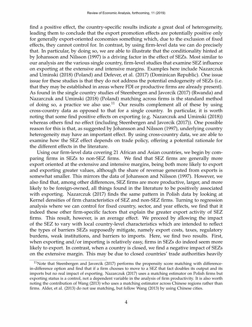
This should not, however, be interpreted as no significant effect since at the samplemean export costs are zero (by construction). Instead, this should be interpreted asin Figure 1 which plots the difference in the estimated probability of exporting for anSEZ firm relative to a non-SEZ firm (vertical axis), all else equal, across the spectrumof export cost values (horizontal axis). The figure indicates that if in a country exportcosts are low (i.e. the left upper corner) SEZ firms are more likely to export with thereverse found when exporting is expensive (i.e. right bottom corner). At the minimum ofthe export cost measure, the estimated marginal effect is positive and highly significant(with a probability value of 0.004). Likewise, for the maximum export costs, the impactis significantly negative (with a probability value of 0.004). This seemingly paradoxicalresult may be driven by the constrained optimization of trade authorities. When aneconomy is closed, relatively little funding may be available to the officials regulatingexports. Therefore they would have an incentive to focus their efforts in locations wherethe values of production, productivity and exports are particularly high, i.e. SEZs.35

This greater scrutiny within an SEZ may then increase the probability of inspection,increasing the expected need for the appropriate export permits which, particularly inthese countries, are costly. As such, while some aspects of exporting may be reduced bythe SEZ, the fixed cost of doing so may rise. In more open and better funded countries,however, this effect would be smaller as the trade authority casts a wider inspectionnet, allowing the export promoting aspects of SEZs to dominate. Furthermore, theseeffects are economically large. Approximately 40% of firms in low export cost countriesexport. As such, the nearly 0.1 increase for low export cost countries in Figure 1 is a 25%increase in the probability of exporting. At the other end, in high export cost countries,only about 20% of firms export. Therefore the roughly 0.2 reduction would reduce theprobability of exporting by nearly 100%.

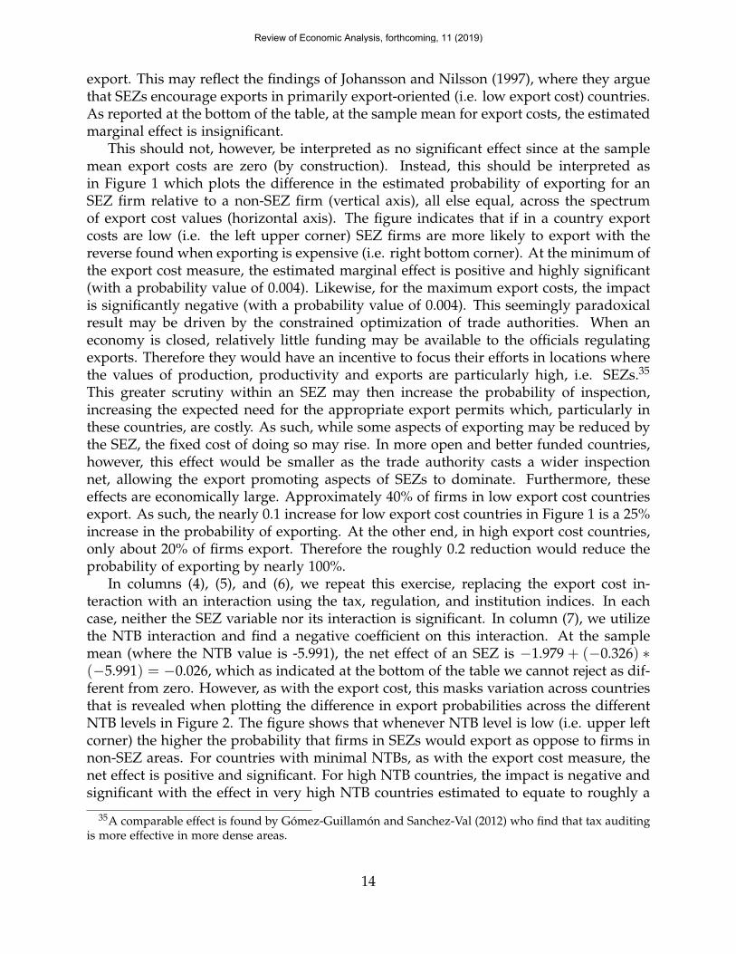
In columns (4), (5), and (6), we repeat this exercise, replacing the export cost in-teraction with an interaction using the tax, regulation, and institution indices. In eachcase, neither the SEZ variable nor its interaction is significant. In column (7), we utilizethe NTB interaction and find a negative coefficient on this interaction. At the samplemean (where the NTB value is -5.991), the net effect of an SEZ is −1.979 + (−0.326) ∗(−5.991) = −0.026, which as indicated at the bottom of the table we cannot reject as dif-ferent from zero. However, as with the export cost, this masks variation across countriesthat is revealed when plotting the difference in export probabilities across the differentNTB levels in Figure 2. The figure shows that whenever NTB level is low (i.e. upper leftcorner) the higher the probability that firms in SEZs would export as oppose to firms innon-SEZ areas. For countries with minimal NTBs, as with the export cost measure, thenet effect is positive and significant. For high NTB countries, the impact is negative andsignificant with the effect in very high NTB countries estimated to equate to roughly a

35A comparable effect is found by Gomez-Guillamon and Sanchez-Val (2012) who find that tax auditingis more effective in more dense areas.

14


Figure 1: Change in the Probability of Exporting - Export Costs

−.2

−.1

0.1

Diff

eren

ce in

Pro

babi

lity

of E

xpor

ting

−2 0 2 4 6Export Costs

95% CI Fitted values

50% reduction in the probability of exporting. Thus, again we see that closed economiesare those where NTBs seem to lower the probability of exporting. Finally, column (8)includes all five interactions where only the export cost and institution coefficients aresignificant. Here, we find that SEZs increase the export probability in countries withweak institutions. In addition, we again find that they reduce the export probabilityin countries with high export costs. Finally, as in column (3), we find a significantlypositive net effect for low export cost countries (with a probability value of 0.001) anda significantly negative effect for high export cost nations (with a probability value of0.0007).

4.2 Propensity Score Matching: Probability of Exporting

Table 6 displays the results of propensity score matching. In Panel A of the table resultswith the unmatched sample indicates that SEZ firms are significantly more likely to ex-port (as in Table 4). However, after matching, i.e. ensuring that probability of treatmentis controlled for, the difference between SEZ and non-SEZ firms is insignificantly nega-tive with a value of τATT = −0.0159. This is in line with the results of Steenbergen andJavorcik (2017) but in contradiction to the matching results from Nazarczuk and Umin-ski (2018) who report τATT = 0.184 which is statistically significant at 1% level. Beyondthe obvious differences in data sets, it should be noted that export barriers in Rwandaare likely large in comparison to the countries in our sample whereas Polish barriers arelikely relatively low. Coming back to our result, the negative differences in the proba-bility of exporting are driven not by a firm being in an SEZ, but by the characteristicsof firms in SEZs. In order to support the validity of this test, Panel B presents threepost-estimation checks, discussed in Caliendo and Koeinig (2008). The first of these is atwo-sample t-test, which works by comparing the means of the covariates between theSEZ and non-SEZ firms, before and after matching. If the matching is of a high qual-

15


Figure 2: Change in the Probability of Exporting - NTBs

−.1

−.0

50

.05

Diff

eren

ce in

Pro

babi

lity

of E

xpor

ting

−7 −6 −5 −4 −3NTBs


ity (i.e. the distribution of treated and control groups are quite similar), no significantdifferences should be found after matching. As the table indicates, it is indeed the case.The second test involves re-estimating the propensity score using the matched sampleand comparing the Pseudo R-squared obtained from the probit estimation before andafter matching. Again, if the matching is of a high quality, the distribution of the co-variates should be similar across treated and untreated firms, resulting in a relativelylow pseudo-R2 after matching has taken place. Again, this holds. Finally, we perform alikelihood test on the joint significance of all the variables included in the probit modelbefore and after matching. Following the same logic, we should expect to reject thistest on the matched sample only (Caliendo and Kopeinig, 2008) which is again the case.Thus, these tests support the validity of the matching.

Combining these results, we see that the impact of SEZs on the probability of export-ing is a nuanced one. In open economies, particularly those generally open to exports,SEZs seem to increase exporting at the extensive margin. For those that are closed toexports and/or imports, however, the opposite effect is found. This is consistent withJohansson and Nilsson (1997) and may be reflective of differences between open andclosed economies with respect to the effectiveness of trade authorities.

16


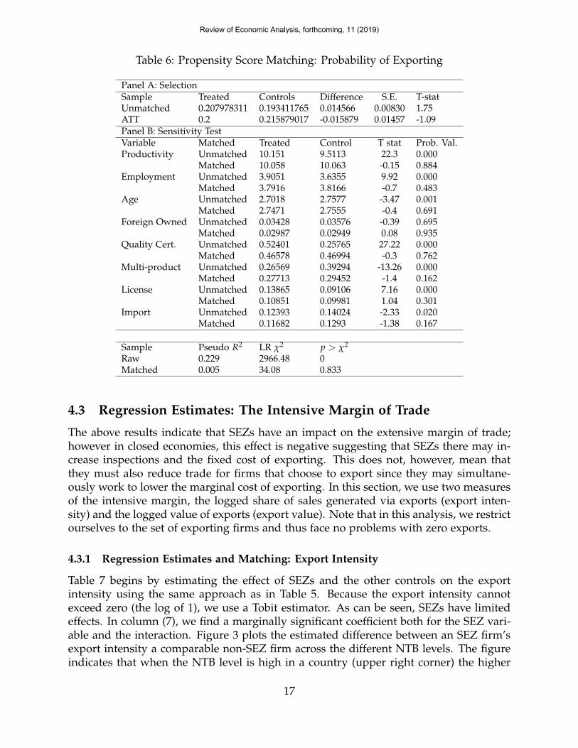
Table 6: Propensity Score Matching: Probability of Exporting

Panel A: SelectionSample Treated Controls Difference S.E. T-statUnmatched 0.207978311 0.193411765 0.014566 0.00830 1.75ATT 0.2 0.215879017 -0.015879 0.01457 -1.09Panel B: Sensitivity TestVariable Matched Treated Control T stat Prob. Val.Productivity Unmatched 10.151 9.5113 22.3 0.000

Matched 10.058 10.063 -0.15 0.884Employment Unmatched 3.9051 3.6355 9.92 0.000

Matched 3.7916 3.8166 -0.7 0.483Age Unmatched 2.7018 2.7577 -3.47 0.001

Matched 2.7471 2.7555 -0.4 0.691Foreign Owned Unmatched 0.03428 0.03576 -0.39 0.695

Matched 0.02987 0.02949 0.08 0.935Quality Cert. Unmatched 0.52401 0.25765 27.22 0.000

Matched 0.46578 0.46994 -0.3 0.762Multi-product Unmatched 0.26569 0.39294 -13.26 0.000

Matched 0.27713 0.29452 -1.4 0.162License Unmatched 0.13865 0.09106 7.16 0.000

Matched 0.10851 0.09981 1.04 0.301Import Unmatched 0.12393 0.14024 -2.33 0.020

Matched 0.11682 0.1293 -1.38 0.167

Sample Pseudo R2 LR χ2 p > χ2

Raw 0.229 2966.48 0Matched 0.005 34.08 0.833

4.3 Regression Estimates: The Intensive Margin of Trade

The above results indicate that SEZs have an impact on the extensive margin of trade;however in closed economies, this effect is negative suggesting that SEZs there may in-crease inspections and the fixed cost of exporting. This does not, however, mean thatthey must also reduce trade for firms that choose to export since they may simultane-ously work to lower the marginal cost of exporting. In this section, we use two measuresof the intensive margin, the logged share of sales generated via exports (export inten-sity) and the logged value of exports (export value). Note that in this analysis, we restrictourselves to the set of exporting firms and thus face no problems with zero exports.

4.3.1 Regression Estimates and Matching: Export Intensity

Table 7 begins by estimating the effect of SEZs and the other controls on the exportintensity using the same approach as in Table 5. Because the export intensity cannotexceed zero (the log of 1), we use a Tobit estimator. As can be seen, SEZs have limitedeffects. In column (7), we find a marginally significant coefficient both for the SEZ vari-able and the interaction. Figure 3 plots the estimated difference between an SEZ firm’sexport intensity a comparable non-SEZ firm across the different NTB levels. The figureindicates that when the NTB level is high in a country (upper right corner) the higher

17


the relative export intensity of an SEZ firm (note that in this and subsequent figures,confidence intervals are included but that they are difficult to see due to the precisenessof the estimates). For open economies (left-hand side of the graph), the point estimate ofthis difference is negative but economically small. For high NTB countries, however, theeffect is significantly positive (with a probability value of 0.049 at the maximum NTB).However, when we also control for export costs in column (8), this effect disappears tobe replaced by a marginally negative coefficient on the interaction between SEZ statusand trade costs. This results in a pattern similar to Figure 1; however it is only for highexport cost countries that we find a significant net effect. That said, as the significanceof the coefficients is not particularly strong, we do not wish to make too much of theseresults, preferring to instead say that the evidence of an SEZ effect on export intensity isat best limited. Other controls do, however, have a strong impact on the export intensity.In particular, younger, single-product, non-importers earn a greater share of sales fromexporting.

Table 7: Export Intensity

VARIABLES(1) (2) (3) (4) (5) (6) (7) (8)

Productivity -0.0349 -0.0368 -0.0364 -0.0369 -0.0377* -0.0369 -0.0392* -0.0396*(0.0224) (0.0225) (0.0225) (0.0225) (0.0225) (0.0225) (0.0225) (0.0227)

Employment 0.0311 0.0314 0.0314 0.0314 0.0322 0.0312 0.0322 0.0342(0.0250) (0.0250) (0.0250) (0.0250) (0.0249) (0.0250) (0.0249) (0.0249)

Age -0.166*** -0.161*** -0.160*** -0.161*** -0.163*** -0.162*** -0.163*** -0.161***(0.0383) (0.0384) (0.0384) (0.0384) (0.0384) (0.0384) (0.0383) (0.0382)

Foreign Owned 0.0858 0.0819 0.0811 0.0836 0.0659 0.0795 0.0748 0.0622(0.116) (0.116) (0.116) (0.117) (0.116) (0.117) (0.116) (0.118)

Quality Cert. -0.0883 -0.0943 -0.0947 -0.0944 -0.0961 -0.0946 -0.0959 -0.102(0.0674) (0.0675) (0.0675) (0.0675) (0.0673) (0.0674) (0.0673) (0.0674)

Multi-product -0.216*** -0.212*** -0.212*** -0.213*** -0.211*** -0.212*** -0.213*** -0.209***(0.0639) (0.0637) (0.0638) (0.0637) (0.0637) (0.0637) (0.0637) (0.0641)

License 0.0769 0.0736 0.0728 0.0733 0.0772 0.0737 0.0768 0.0760(0.0780) (0.0779) (0.0779) (0.0780) (0.0781) (0.0779) (0.0780) (0.0779)

Import -0.121* -0.123* -0.122* -0.122* -0.127* -0.124* -0.128* -0.124*(0.0669) (0.0667) (0.0668) (0.0668) (0.0666) (0.0667) (0.0666) (0.0664)

SEZ 0.0940 0.0904 0.00687 1.026 0.226 1.454* 2.895*(0.0730) (0.0728) (0.477) (0.652) (0.497) (0.782) (1.515)

Export costs*SEZ -0.0339 -0.224*(0.0691) (0.131)

Taxes*SEZ -0.0214 -0.0765(0.117) (0.373)

Regulation*SEZ 0.165 0.134(0.114) (0.360)

Institutions*SEZ 0.0240 -0.0615(0.0884) (0.155)

NTBs*SEZ 0.222* 0.445(0.126) (0.317)

Constant -0.822** -0.852** -0.821** -0.811** -1.006** -0.911** -0.764** -0.295(0.363) (0.367) (0.365) (0.390) (0.391) (0.413) (0.365) (0.420)

Net SEZ effect=0 0.21 0.21 0.17 0.19 0.11 0.23Observations 2,291 2,291 2,291 2,291 2,291 2,291 2,291 2,291Notes: ***, **, and * on difference denote significance at the 1%, 5%, and 10% levels respectively. All specifications include country,sector and year dummies. Net SEZ Effect = 0 reports the p value at the sample mean.

As with the extensive margin, one might worry about the endogeneity of the SEZvariable, thus in Table 8 we employ the same matching technique described above (but

18


Figure 3: Change in Intensity of Exporting - NTBs

0.2

.4.6

.8D

iffer

ence

in E

xpor

t Int

ensi

ty

−7 −6 −5 −4 −3NTBs


Note: 95% Confidence Intervals are extremely narrow andhence indistringuishable from the line.

replacing the exporter dummy with the export intensity variable). Here, as we havefewer exporting firms we are forced to rely on a set of 821 non-SEZ firms and 158SEZ firms for which we had common support. As in the extensive margin results,after matching we estimate an insignificant τATT = 0.1433 with the post-estimation testssupporting the quality of the matches. That is in line with Nazarczuk and Uminski(2018). Thus, after other important firm characteristics are matched, the export intensityof SEZ and non-SEZ firms are statistically the same.

4.3.2 Regression Estimates and Matching: Export Value

Table 9 turns to the Export Value (again for the set of exporting firms). As with theexport intensity results, we find limited impact of SEZs. That said, we do find a rela-tively robust impact from the NTB interaction which is significantly positive, both onits own in column (7) and when used alongside the other interactions in column (8).Figure 4 illustrates the estimated impact. The figure indicates that whenever NTB levelis high (i.e. closed economies) the higher the difference in export sales level betweenfirms in SEZs,and those in non-SEZ parts (upper right corner). Comparable to Figure3, we find no economically significant effect for low NTB countries but an economicallyand statistically significant positive effect in high NTB countries. At that end of the NTBdistribution, the expected difference in exports is 0.5 which, relative to the mean exportvalue of 13.7 in high NTB countries, is a 3.6% increase. This may be evidence of the factthat it is possible for SEZ firms to import intermediates under reduced duties, increas-ing production and therefore exports. In addition, column (5) provides some marginalevidence that SEZ increase export volumes in strong regulation countries, with the ef-

19


fect illustrated in Figure 5. The figure suggests that at highly regulated economies thedifference in export volumes become more apparent between firms in SEZs and thosein non-SEZ parts where SEZ firms making more export sales. Again, it is only for theheavily regulated countries where we estimate an economically significant net effect, onewhich indicates that SEZ firms in these nations export a greater value. Beyond the SEZvariable, unsurprisingly, more productive, larger, and foreign firms export higher values.Younger, single-product, and non-importing firms also export greater values.

Finally, Table 10 again explores the possibility that our results are driven by endo-geneity of the SEZ variable. Nevertheless, we again find an insignificant effect aftermatching, with τATT = 0.0212. As with the extensive margin, this is consistent withexport value results of Steenbergen and Javorcik (2017) but differs from those Nazarczukand Uminski (2018). Note that, as this is the same set of firms as in Table 8 with a dif-ferent export outcome variable, the post-estimation tests from matching are the same asreported there.

Table 8: Propensity Score Matching: Export Intensity

Panel A: SelectionSample Treated Controls Difference S.E. T-statUnmatched -1.17866516 -0.823489372 -0.355175786 0.052534604 -6.76ATT -1.14432697 -1.28757787 0.143250898 0.141142051 1.01Panel B: Sensitivity TestVariable Treated Control T stat Prob. Val.Productivity Unmatched 10.46 9.7555 10.68 0.000

Matched 10.357 10.496 -0.89 0.375Employment Unmatched 4.7738 4.9919 -3.41 0.001

Matched 4.884 4.6757 1.40 0.164Age Unmatched 2.8231 2.9316 -3.04 0.002

Matched 2.8858 2.9854 -1.20 0.232Foreign Owned Unmatched .10056 .07186 2.19 0.029

Matched .10759 .06329 1.41 0.160Quality Cert. Unmatched .69646 .4933 9.17 0.000

Matched .72152 .64557 1.45 0.148Multi-product Unmatched .26536 .42144 -7.24 0.000

Matched .25949 .24684 0.26 0.797License Unmatched .19646 .19732 -0.05 0.963

Matched .23418 .20886 0.54 0.589Import Unmatched .3473 .36784 -0.93 0.355

Matched .3481 .33544 0.24 0.813

Sample Pseudo R2 LR χ2 p > χ2

Raw 0.232 601.61 0Matched 0.092 39.18 0.179

20


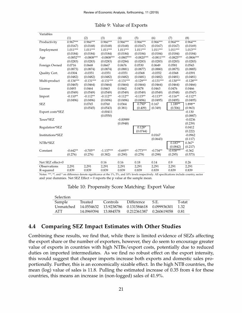
Table 9: Value of Exports

Variables(1) (2) (3) (4) (5) (6) (7) (8)

Productivity 0.967*** 0.966*** 0.966*** 0.966*** 0.966*** 0.966*** 0.964*** 0.964***(0.0167) (0.0168) (0.0168) (0.0168) (0.0167) (0.0167) (0.0167) (0.0169)

Employment 1.011*** 1.011*** 1.011*** 1.011*** 1.011*** 1.011*** 1.011*** 1.013***(0.0184) (0.0184) (0.0184) (0.0184) (0.0184) (0.0184) (0.0184) (0.0184)

Age -0.0852*** -0.0808*** -0.0808*** -0.0807*** -0.0820*** -0.0811*** -0.0825*** -0.0806***(0.0283) (0.0283) (0.0283) (0.0284) (0.0283) (0.0283) (0.0283) (0.0283)

Foreign Owned 0.0716 0.0668 0.0667 0.0676 0.0530 0.0649 0.0581 0.0543(0.0873) (0.0874) (0.0874) (0.0881) (0.0877) (0.0880) (0.0875) (0.0885)

Quality Cert. -0.0304 -0.0351 -0.0351 -0.0351 -0.0368 -0.0352 -0.0368 -0.0391(0.0482) (0.0482) (0.0482) (0.0482) (0.0481) (0.0482) (0.0481) (0.0481)

Multi-product -0.134*** -0.131*** -0.131*** -0.131*** -0.129*** -0.131*** -0.130*** -0.128***(0.0465) (0.0464) (0.0464) (0.0464) (0.0464) (0.0464) (0.0464) (0.0466)

License 0.0493 0.0464 0.0463 0.0462 0.0478 0.0463 0.0476 0.0466(0.0549) (0.0549) (0.0549) (0.0549) (0.0549) (0.0549) (0.0548) (0.0547)

Import -0.110** -0.112** -0.112** -0.112** -0.115** -0.113** -0.116** -0.112**(0.0496) (0.0496) (0.0496) (0.0496) (0.0496) (0.0495) (0.0495) (0.0495)

SEZ 0.0765 0.0760 0.0364 0.790* 0.167 1.189** 1.898**(0.0545) (0.0543) (0.381) (0.409) (0.349) (0.506) (0.963)

Export costs*SEZ -0.00411 -0.130(0.0550) (0.0887)

Taxes*SEZ -0.00989 -0.0236(0.0948) (0.239)

Regulation*SEZ 0.128* 0.0412(0.0744) (0.222)

Institutions*SEZ 0.0167 -0.0962(0.0643) (0.117)

NTBs*SEZ 0.183** 0.367*(0.0842) (0.217)

Constant -0.642** -0.705** -1.137*** -0.695** -0.773*** -0.734** -0.938*** -0.362(0.276) (0.276) (0.382) (0.290) (0.278) (0.298) (0.295) (0.573)

Net SEZ effect=0 0.16 0.16 0.18 0.14 0.9 0.26Observations 2,291 2,291 2,291 2,291 2,291 2,291 2,291 2,291R-squared 0.839 0.839 0.839 0.839 0.839 0.839 0.839 0.839Notes: ***, **, and * on difference denote significance at the 1%, 5%, and 10% levels respectively. All specifications include country, sectorand year dummies. Net SEZ Effect = 0 reports the p value at the sample mean.

Table 10: Propensity Score Matching: Export Value

SelectionSample Treated Controls Difference S.E. T-statUnmatched 14.0554632 13.9238786 0.131584618 0.099936301 1.32ATT 14.0969394 13.884578 0.212361387 0.260619058 0.81

4.4 Comparing SEZ Impact Estimates with Other Studies

Combining these results, we find that, while there is limited evidence of SEZs affectingthe export share or the number of exporters, however, they do seem to encourage greatervalue of exports in countries with high NTBs/export costs, potentially due to reducedduties on imported intermediates. As we find no robust effect on the export intensity,this would suggest that cheaper imports increase both exports and domestic sales pro-portionally. Further, this is an economically sizable effect. In the high NTB countries, themean (log) value of sales is 11.8. Pulling the estimated increase of 0.35 from 4 for thesecountries, this means an increase in (non-logged) sales of 41.9%.

21


Figure 4: Change in Value of Exports - NTBs

−.2

0.2

.4.6

Diff

eren

ce in

Exp

ort V

alue

−7 −6 −5 −4 −3NTBs



Because the interaction with these trade barrier measures is our innovation, there areno comparable results in the literature for us to compare ourselves to. Nevertheless, it isinstructive to compare what is comparable (the non-interacted SEZ dummy in column2 of Tables 5 (probability of exporting) and 9 (export value)). In Table 11, we compareour estimates with those in Nazarczuk and Uminski (2018), Steenbergen and Javorcik(2017), and Nesterenko (2003). While there are differences across the studies, all, usefirm-level data, employ and exporter dummy (using a Logit estimator) or logged ex-port values (with OLS), and include an SEZ dummy as the variable of interest. However,there are differences in terms of time, country coverage and the size of samples as shownin the table. Despite these difference, as reported, the various studies all find positivecoefficents for the SEZ dummy at both level extensive and intensive margins. Overall,the magnitude of our estimates fall somewhere in the middle with those reported byNazarczuk and Uminski (2018) notably higher which might be due to the overall open-ness of Poland compared to the countries in the other three studies. In general, we findthat our estimates are generally in line with those found elsewhere which suggests that,across the literature while SEZs do not negatively impact firms’ exporting behavior, theirvalue as an export-promoting policy tool can be questioned.

22


Figure 5: Change in Value of Exports - Regulation

−.1

0.1

.2.3

.4D

iffer

ence

in E

xpor

t Val

ue

−7 −6 −5 −4 −3Regulation



Table 11: Extensive and Intensive Margin Estimates Compared

Nazarczuk Steenbergena Nesterenkob (2003) Ourc

& Uminski (2018) & Javorcik (2017) Results

Dep. Var. — Exporter (dummy) Exporter (dummy) Exporter (dummy) Exporter (dummy)

SEZ — 1.124 0.0079 0.48311*** 0.0115

Dep. Var. — Export Value (log) Export Value (log) Export Value (log) Export Value (log)

SEZ — 1.740*** 0.159 0.067*** 0.0765

Data — Firm-level Firm-level Firm-level Firm-levelObs. — 518 179,149 23,649 11,161/ 2,291Period(s) — 2004-2014 2008-2016 1996-1999 2007-2014Sector(s) — Mnfc. Mnfc & Srvs Mnfc. 22 Mnfc.Country(ies) — Poland Rwanda Ukraine 21 African/AsianEst. method — Logit/OLS-FE Logit/OLS-FE-DiD Logit/OLS-FE Logit/OLS-FENotes: ***, **, and * on difference denote significance at the 1%, 5%, and 10% levels.a They use quarterly firm reports in and outside of SEZs in Kigali, Rwanda.b Dataset covers 24 counties in Ukraine.c Our dataset is a cross-sectional one consolidating surveys conducted at some point in 2007-14 period

4.5 Additional Regressions

To explore the data further, we examined several alternative samples. First, rather thanmanufacturing, we considered agricultural products. There, as in manufacturing, we

23


found only occasionally significant impacts of SEZs and when this was the case, theywere typically negative and then for the extensive margin. Second, we considered differ-ent subsamples of manufacturing, specifically food, transport equipment, and textiles.Although the significance of the coefficients was markedly weaker, potentially due tothe smaller sample sizes, when the SEZ variables were significant, they were compara-ble to those found here. As a further test of the endogeneity of the SEZ variable, fol-lowing the results of Ebenstein (2012), we split the sample between foreign-owned anddomestically-owned firms since he found that the first group was more likely to locate inan SEZ than elsewhere. Nevertheless, we found the same results in these subsamples asin the combined sample, again suggesting that endogeneity is not driving the result. Weestimated the effect of SEZs separately for Asian and African countries (the two groupsin our data) and excluding India (which represents a large share of the sample). In bothcases, neither the SEZ variable itself nor its interactions were significant. We also tried tointeract importer dummy with the NTB and export cost variables.36 When doing so, wefind that importers in SEZs have a smaller impact from NTBs on their exporting behaviorat both margins, suggestive that SEZs might help to mitigate some of the trade barriersfelt by importers who also wish to export. Finally, in our intensive margin regressions,we explored the potential role of the WTO’s Export Share Requirement (ERS) policy.37.This policy demands that, to be consistent with WTO rules, firms in SEZs should berequired to achieve a minimum export intensity (Defever and Riano, 2017). In Table 4,we show that the export share of SEZ firms is instead smaller than for non-SEZ ones,suggesting a contradiction of the ERS policy. Delving deeper, this difference is driven bytwo countries, Zimbabwe and South Africa.38 That said, after dropping these two coun-tries, our results do not change significantly. All of these additional results are availableon request.

5 Conclusion

Special economic zones have long been touted as a method of increasing exports and,as a result, improving the level of development in a region. While there are numer-ous case studies on the issue, there is scant econometric evidence testing the notion.We contribute to the debate by providing the first firm-level, cross-country econometricstudy testing whether SEZs do in fact increase exports at either the extensive or inten-sive margins. The resulting pattern is a nuanced one. At the extensive margin, SEZsincrease the likelihood of exporting by as much as 25%, but only for firms in relativelyopen economies. In closed economies, we find the opposite effect, something that mightbe consistent with differing patterns of enforcement across countries. At the intensivemargin, we find little evidence suggesting that SEZs affect the share of sales earned

36This was motivated in part by Yang, et al. (2011) who find that firms choose to move to SEZs inChina because they import raw materials and intermediates. Thus, the import duty reductions in the SEZsignificantly lower importers’ production costs.

37We thank one of our reviewers for suggesting this.38Those countries might have removed the ERS policy to attract more FDI to their SEZs as done by the

Dominican Republic (Defever, et al. 2017).

24


from exporting. They do, however, seem to markedly increase the value of exports incountries with import barriers, something that suggests that SEZs may reduce the costof intermediate inputs, encouraging both domestic and foreign sales. Combining theseeffects, if the goal is to increase exporting, it is likely that policy makers will need toconsider SEZs in light of the local economic environment before choosing to use them.This is consistent with the other single-country studies on SEZs and, as indicated inYang, et al. (2011), it may suggest that the additional costs of being in an SEZ (e.g.higher fixed setup costs) can outweigh their benefits. That said, our results do indicate aconditional effectiveness of SEZs and future research with access to panel data can helpto fill out the policy environment for which they do (or do not) promote exporting. Inparticular, our estimates suggest that in open economies, SEZs affect the extensive mar-gin positively with little effect on the intensive margin whereas for closed economies,introducing SEZs may mean greater exports spread across fewer firms. As these havedistributional consequences across firms and regions, such factors should be consideredwhen creating SEZs. As such, we hope that our results provide a stepping stone to thedevelopment of a framework under which SEZs play a useful role in a general overhaulof a country’s policies.

25


References

[1] Aggarwal, A. (2004), Export Processing Zones in India: Analysis of the ExportPerformance. Working Paper No 148, Indian Council for Research on InternationalEconomic Relations.

[2] Alder, S., Shao, L. and Zilibotti, F. (2013), The Effect of Economic Reform and In-dustrial Policy in a Panel of Chinese Cities. Working Paper N 207, University ofZurich.

[3] Amirahmadi, H. and Wu, W. (1995), Export Processing Zones in Asia. Asian Survey,35(9), 828-849.

[4] Brautigam, D. and Tang, X. (2014), Going Global in Groups: Structural Transforma-tion and China’s Special Economic Zones Overseas. World Development, 63, 78-91.

[5] Busso, M., Gregory, J., Patrick, K. (2013), Assessing the Incidence and Efficiency ofa Prominent Place Based Policy. American Economic Review, 103(2), 897-947.

[6] Caliendo, M. and Kopeinig, S. (2008), Some Practical Guidance for the Implemen-tation of propensity Score Matching. Journal of Economic Surveys. 22(1), pp. 31-72.

[7] Chaudhuri, S. and Yabuuchi, S. (2010), Formation of Special Economic Zones, Liber-alized FDI Policy and Agricultural Productivity. International Review of Economicsand Finance, 19, 779-788.

[8] Davies, R.B. and Jeppesen, T. (2015), Export Mode, Trade Costs, and ProductivitySorting. Review of World Economics, 151(2), 169-195.

[9] Davies, R.B. and Mazhikeyev, A. (2015), The Glass Border: Gender and Exportingin Developing Countries. Mimeo.

[10] Defever, F., Reyes, J., Riano, A. and Sanchez-Martin, M. E. (2017), Special EconomicZones and WTO Compliance: Evidence from the Dominican Republic. CEP Discus-sion Paper No 1517, Centra for Economic Performance.

[11] Defever, F. and Riano, A. (2015), Protectionism Through Exporting: Subsidies withExport Share Requirements in China. Mimeo.

[12] Devereux, J. and Chen, L. L. (1995), Export zones and welfare: Another look. OxfordEconomic Papers, 47, 704-713.

[13] Din, M. (1994), Export Processing Zones and Backward Linkages. Journal of Devel-opment Economics, 43, 369-385.

[14] Ebenstein, A. (2012), Winners and Losers of Multinational Firm Entry into Develop-ing Countries: Evidence from the Special Economic Zones of the Peoples Republicof China. Asian Development Review, 29(1), 29-56.

26


[15] The Economist. (2015), Special Economic Zones: Not So Special. April 3, 2015.

[16] Elliott, R. and Virakul, S. (2010), Multi-Product Firms and Exporting: A DevelopingCountry Perspective. Review of World Economics, 146, 635-656.

[17] Farole, T. (2011), Special Economic Zones in Africa: Comparing Performance andLearning from Global Experiences. The World Bank: Washington D.C.

[18] Farole, T. and Akinci, G. (2011), Special Economic Zones: Progress, Emerging Chal-lenges, and Future Directions. The World Bank: Washington D.C.

[19] Fraser Institute. (2014), Economic Freedom of the World. Fraser Institute: Vancou-ver.

[20] Ge, W. (1999), Special Economic Zones and the Opening of the Chinese Economy:Some Lessons for Economic Liberalization. World Development, 27(7), 1267-1285.

[21] Gomez-Guillamon, A. and Sanchez-Val, M. (2012), The Geographical Factor in theDetermination of Audit Quality. Revista de Contabilidad, 15(2), 287-310.

[22] Hamilton, C. and Svennson, L. (1982), On the Welfare Effects of a Duty-Free Zone.Journal of international Economics, 13, 45-64.

[23] Jensen, C. and Winiarczyk, M. (2014), Special Economic Zones: 20 Years Later. Cen-ter for Social and Economic Research Working Paper No. 467.

[24] Johansson, H. and Nilsson, L. (1997), Export Processing Zones as Catalysts, 25(12),2115-2128.

[25] Kline, P., (2010), Place based policies, heterogeneity, and agglomeration. AmericanEconomic Review: Papers and Proceedings, 100 (2), 383-387.

[26] Leong, C.K. (2013), Special economic zones and growth in China and India: anempirical investigation. International Economics and Economic Policy, 10(4), 549-567.

[27] Madani, D. (1999), A Review of the Role and Impact of Export Processing Zones.World Bank Policy Research Working Paper 2238.

[28] McCann, F. (2013), Indirect Exporters. Journal of Industry, Competition and Trade,13(4), 519-535.

[29] Melitz, M. and Ottaviano, G. (2008), Market Size, Trade and Productivity. Reviewof Economic Studies, 75(1), 295-316.

[30] Melitz, M. (2003), The Impact of Trade on Intra-Industry Reallocations and Aggre-gate Industry Productivity. Econometrica, 71(6), 1695-1725.

[31] Miyagiwa, K. (1986), A reconsideration of the welfare economics of the free tradezone. Journal of International Economics, 21, 337-350.

27


[32] Miyagiwa, K. (1993), The locational choice for free trade zones: Rural versus urbanoptions. Journal of Development Economics, 40, 187-203.

[33] Nazarczuk, J. M. and Uminski, S. (2018), The Impact of Special Economic Zones onExport Behavious. Evidence from Polish Firm-level Data. Ekonomie. XXI(3), 1-22.

[34] Nazarczuk, J. M. (2017), Do operations in SEZs improve a firm’s productivitiy?Evidence from Poland. New Trends and Issues Proceedings on Humanities andSocial Sciences, [Online]. 4(10), 256-264. Available from: www.prosoc.eu

[35] Nesterenko, A. (2003), The Determinants of Firms’ Export Behavior. MSc Thesis, Na-tional University of “Kyiv-Mohyla Academy” Economics Education and ResearchConsortium.

[36] Pavcnik, N. (2002), Trade liberalization, exit and productivity improvements: evi-dence from Chilean plants. The Review of Economic Studies, 69(1), 245276.

[37] Schweinberger, A. G. (2003), Special Economic Zones in Developing and/or Transi-tion Economies: A Policy Proposal. Review of International Economics, 11, 619-629.

[38] Steenbergen, V. and Javorcik, B. (2017), Analysing the impact of the Kigali SpecialEconomic Zone on firm behaviour. Working Paper F-38419-RWA-1, InternationalGrowth Centre.

[39] Wang, J. (2013), The economic impact of Special Economic Zones: Evidence fromChinese municipalities. Journal of Development Economics, 101, 133-147.

[40] World Bank. (2008), Special Economic Zones: Performance, Lessons Learned, andImplications for Zone Development. The World Bank: Washington D.C.

[41] World Economic Forum. (2014), The Global Competitiveness Report. PalgraveMacMillan: Geneva.

[42] Yabuuchi, S. (2000), Export processing zones, backward linkages, and variable re-turns to scale. Review of Development Economics, 4, 268-278.

[43] Yang, X., Wang, Z., Chen, Y. and Yuan, F. (2011), Factors Affecting Firm-level In-vestment and Performance in Border Economic Zones and Implications for Devel-oping Cross-Border Econmic Zones between the People’s Republic of China andits Neighboring GMS Countries. Research Report Series, Volume 1, Issue 1, AsianDevelopment Bank.

[44] Yucer, A. and Siroen, J-M. (2017), Trade Performance of Export Processing Zones.The World Economy, doi: 10.1111/twec.12395

[45] Zeng, D.Z. (2015), Global Experiences with Special Economic Zones: Focus onChina and Africa. The World Bank: Washington D.C.

28
