THE PERFORMANCE OF RENEWABLE PORTFOLIO STANDARDS

IN THE UNITED STATES

By

Binlei Gong

A THESIS

Submitted to

Michigan State University

in partial fulfillment of the requirements

for the degree of

MASTER OF SCIENCE

Agricultural, Food and Resource Economics

2011

ABSTRACT

THE PERFORMANCE OF RENEWABLE PORTFOLIO STANDARDS

IN THE UITED STATES

By

Binlei Gong

The Renewable Portfolio Standard (RPS) is a renewable energy policy that ensures a minimum

amount of renewable energy in the portfolio of electric-generating resources serving a state. This

article first analyzes theoretically expected effects of RPS on renewable energy quantities,

electricity price, and emissions. With a balanced panel of 48 states for 1990-2008, this paper

estimates causal impact of RPS through an econometric model. During these regressions, a new

measure for RPS indicator has also been introduced to deal with the heterogeneity problem. This

paper also account for the partial effect and the different trends of outcomes in the absence of RPS

across states. The estimators imply that RPS on average are effective in having a positive impact

on renewable energy share but not that efficient since significantly increasing the electricity price.

This research also finds that strengthening RPS can reduce carbon and other emissions but these

benefits cannot fully compensate the consumer surplus loss caused by RPS, which finally implies a

national-wide RPS is likely to be inefficient even with emission concern. Finally, the

breakeven price is estimated, which implies the policies‘ cost of reducing the emissions. This

paper also does same analysis on regional level and concludes that RPS is likely to be efficient in

Midwest and in West but not that efficient in Northeast and in South with emission concern.

Copyright by

Binlei Gong

2011

iv

This thesis is dedicated to my dear parents and to my grandfather in heaven.

谨以此文献给我亲爱的父母以及远在天堂的爷爷。

v

ACKNOWLEDGEMENTS

The completion of this thesis is a perfect ending for my two years graduate study at

Michigan State University. It is my honor to be a member of the big family in the Department

of Agricultural, Food and Resource Economics. I will never forget my friends and professors

who studied and worked with me during the past 700 days.

First and foremost, I would like to especially thank my major professor, Dr. Jinhua Zhao,

for his guidance to my research. I appreciate the initial research idea that he provided in 2009

as well as his continuous support since then.

I‘d like to also thank members of my thesis committee, Dr. Soren Anderson and Dr.

Thomas Dietz. They are the top researchers in Economics and Sociology, respectively. Dr.

Anderson taught me a lot in the AEC835 econometrics class and gave me many suggestions on

the empirical model in Section 4 of this thesis. Dr. Thomas Dietz provided me a whole page of

study on climate change in the ESP 891 climate change and society course and the thoughts of

environment concern of evaluating the policy in Section 4 and 6.

I am also grateful to the help of Dr. David Schweikhardt, who introduced the SSP analysis

in EC 810 Institutional Economics class and instructed its specific application in my research in

Section 3, Dr. Wooldridge, who gave suggestions on the econometric model with a different

trends concern, and Dr Lindon Robison, who helped build my mathematical foundation to do the

thesis through the calculus and statistics classes.

vi

Thank you to David Perry for offering the Sierra Club member statistics information.

Thank you to Dr. Lester Yuan from EPA for providing useful advice about my model. Thank

you to Dr. Min Wang for being an amazing source of inspiration and comments.

Finally, I thank you to my family especially my father and mother for being my base, both

mentally and financially. I miss you so much and would like to see you as soon as possible. I

also give my best wish to my grandfather who passed away at the end of 2009 when I was in

United States.

vii

TABLE OF CONTENTS

LIST OF TABLES ......................................................................................................................... ix

LIST OF FIGURES ........................................................................................................................ x

LIST OF ABBREVIATIONS ....................................................................................................... xii

CHAPTER 1: INTRODUCTION ................................................................................................... 1

CHAPTER 2: BACKGROUND ..................................................................................................... 5

2.1 Overview of RPS policies in the United States ........................................................................... 5

2.2 Features of RPS Policies ................................................................................................................. 9

2.3 How It Works: Rights and Duties in RPS Institution ............................................................... 11

2.4 Previous Literature on RPS Impacts and Effectiveness............................................................ 12

2.5 Development of RPS and Selected Variables ............................................................................ 15

2.5.1 Northeast vs. Midwest vs. South vs. West ................................................................... 17

2.5.2 Early-RPS States vs. Late- RPS States vs. Non-RPS States ........................................ 19

2.5.3 Low vs. Medium vs. High States in Renewable Energy Potentials ............................. 23

2.5.4 Before vs. After the deployment of RPS ...................................................................... 33

2.5.5 Features in Each States ................................................................................................. 36

2.6 Other Policies for Renewable Energy ......................................................................................... 38

CHAPTER 3: CONCEPTUAL MODEL...................................................................................... 39

3.1 Effect on Renewable Energy Share in Capacity and Generation ............................................ 40

3.1.1 Situation: Renewable Energy as Economies of Scale Good ........................................ 40

3.1.2 Structure and Performance: A1, A2, A3 and P1, P2, P3 .............................................. 40

3.2 Effect on Electricity Price ............................................................................................................. 44

3.2.1 Situation: Air as an Incompatible Use Good ................................................................ 44

3.2.2 Structure and Performance: A4, A5, A6 and P4, P5, P6 .............................................. 45

3.3 Effect on Emissions ....................................................................................................................... 48

3.4 Conclusion and Hypotheses ......................................................................................................... 50

CHAPTER 4: EMPIRICAL MODEL .......................................................................................... 52

4.1 Effect on Renewable Energy Share and Electricity Price ........................................................ 52

4.1.1 Basic LSDV Model ...................................................................................................... 52

4.1.2 Potential Problem of the Basic Model and Solutions ................................................... 55

4.1.3 Prediction of RPS Impacts ............................................................................................ 60

4.1.4 Conclusion .................................................................................................................... 61

viii

4.2 RPS Impacts on Consumer Surplus, Emissions, and Total Consumer Welfare .................... 62

4.2.1 Effect on Consumer Surplus ......................................................................................... 64

4.2.2 Effect on Emissions ...................................................................................................... 67

4.2.3 Conclusion .................................................................................................................... 71

CHAPTER 5: DATA DESCRIPTION ......................................................................................... 74

CHAPTER 6: ESTIMATION RESULTS .................................................................................... 81

6.1 Prediction on Renewable Energy share and Electricity Price .................................................. 81

6.1.1 Estimations for All the 48 Lower States ....................................................................... 81

6.1.2 Estimations for Each of the Four Regions .................................................................... 90

6.1.3 Conclusion .................................................................................................................... 97

6.2 Prediction on Consumer Surplus Loss ........................................................................................ 99

6.2.1 Demand Elasticity for Electricity Market ..................................................................... 99

6.2.2 Consumer‘s Surplus Loss ........................................................................................... 101

6.3 Prediction on Reduced Emission and Its Value .......................................................................102

6.3.1 Reduced Emissions Amount ....................................................................................... 102

6.3.2 The Value of Reduced Emissions ............................................................................... 106

6.4 Total Welfare for Consumers .....................................................................................................109

6.4.1 Estimations for All the 48 Lower States ..................................................................... 109

6.4.2 Estimations for Each of the Four Regions .................................................................. 111

CHAPTER 7: CONCLUSION ................................................................................................... 114

APPENDIX ................................................................................................................................. 116

Appendix 1: Equations for every column of Table 6.1, Table 6.2, and Table 6.3 .....................117

Appendix 2: Testing for Serial Correlation of Equation (2) in Appendix 1 ...............................118

Appendix 3: Testing for Serial Correlation of Equation (2*) in Appendix 1 ............................119

Appendix 4: Testing for Serial Correlation of Equation (2**) in Appendix 1 .........................120

Appendix 5: Testing for Serial Correlation of Equation (5*) in Appendix 1 ............................121

Appendix 6: Testing for Serial Correlation of Equation (3) in Appendix 1 ...............................122

Appendix 7: Testing for Serial Correlation of Equation (3*) in Appendix 1 ............................123

Appendix 8: Testing for Serial Correlation of Equation (3**) in Appendix 1 .........................124

Appendix 9: Testing for Serial Correlation of Equation (6*) in Appendix 1 ............................125

Appendix 10: Testing for Serial Correlation of Equation (4) in Appendix 1 .............................126

Appendix 11: Testing for Serial Correlation of Equation (4*) in Appendix 1 ..........................127

Appendix 12: Testing for Serial Correlation of Equation (4**) in Appendix 1 .......................128

Appendix 13 Testing for Serial Correlation of Equation (7*) in Advanced Model .................129

BIBLIOGRAPHY ....................................................................................................................... 130

ix

LIST OF TABLES

Table 1.1 State mandatory RPS schedule and target ....................................................................... 2

Table 2.1 Groups that each state belongs to .................................................................................. 36

Table 3.1 SSP analysis matrix: renewable energy as Economies of Scale Goods ........................ 43

Table 3.2 SSP analysis matrix: Air as an Incompatible Use Good ............................................... 47

Table 3.3 Caparison among non-RPS states, RPS states without and with REC market ............. 50

Table 5.1 Summary statistics ........................................................................................................ 74

Table 6.1 OLS regression results of the capacity equations for all the 48 states .......................... 82

Table 6.2 OLS regression results of the generation equations for all the 48 states ...................... 84

Table 6.3 OLS regression results of the price equations for all the 48 states ............................... 86

Table 6.4 OLS regression results for Northeast and for Midwest ................................................. 91

Table 6.5 OLS regression results for South and for West ............................................................. 94

Table 6.6 Conclusion of the OLS estimators ................................................................................ 97

Table 6.7 OLS and TSLS estimates for demand function with RPS annual target as an IV ...... 100

Table 6.8 Energy share and unit emission estimates in electricity industry by source ............... 104

Table 6.9 Consumer welfare change and breakeven price for carbon for all the states ............... 110

Table 6.10 Consumer welfare change and breakeven price for carbon for each region .............. 112

Table A.1 Equations for every column of Table 6.1, Table 6.2, and Table 6.3 ............................ 117

x

LIST OF FIGURES

Figure 2.1 State Renewable Portfolio Standard and renewable portfolio goals ............................. 6

Figure 2.2 State RPS timeline and coverage of population and electricity generation ................... 8

Figure 2.3 RPS annual target and key variables for 48 lower states ............................................. 16

Figure 2.4 RPS annual target and key variables for each region .................................................. 18

Figure 2.5 RPS annual target and key variables for early-RPS, late-RPS, and non-RPS state .... 20

Figure 2.6 Comparison in key variables among early-, late-, and never-adopters ....................... 21

Figure 2.7 RPS annual target and key variables for low-, medium-, and high-solar states .......... 25

Figure 2.8 Comparison in key variables among low-, medium-, and high-solar states ................ 26

Figure 2.9 RPS annual target and key variables for low-, medium-, and high-biomass states ..... 28

Figure 2.10 Comparison in key variables among low-, medium-, and high-biomass states ........ 29

Figure 2.11 RPS annual target and key variables for low-, medium-, and high-wind states ........ 31

Figure 2.12 Comparison in key variables among low-, medium-, and high-wind states ............. 32

Figure 2.13 RPS annual target and key variables before and after the deployment of RPS ......... 35

Figure 3.1 Energy generation as economy of scale goods ............................................................ 41

Figure 3.2 Demand and supply of electricity market before and after the deployment of RPS ... 48

Figure 4.1 Procedures of estimating consumer‘s total welfare ..................................................... 63

Figure 4.2 Pie Chart of Energy Consumption by Fuel Source ..................................................... 69

Figure 4.3 Energy Consumption Ratio Tendency by Fuel Source from 1990 to 2008 ................. 70

xi

Figure A.1 The relation between residuals and their lagged values in equation (2) .................... 118

Figure A.2 The relation between residuals and their lagged values in equation (2*) ................. 119

Figure A.3 The relation between residuals and their lagged values in equation (2**) .............. 120

Figure A.4 The relation between residuals and their lagged values in equation (5*) ................ 121

Figure A.5 The relation between residuals and their lagged values in equation (3) ................... 122

Figure A.6 The relation between residuals and their lagged values in equation (3*) ................ 123

Figure A.7 The relation between residuals and their lagged values in equation (3**) .............. 124

Figure A.8 The relation between residuals and their lagged values in equation (6*) ................ 125

Figure A.9 The relation between residuals and their lagged values in equation (4) ................... 126

Figure A.10 The relation between residuals and their lagged values in equation (4*) .............. 127

Figure A.11 The relation between residuals and their lagged values in equation (4**) ............ 128

Figure A.12 The relation between residuals and their lagged values in equation (7*) .............. 129

xii

LIST OF ABBREVIATIONS

ACP Alternative Compliance Payment

ARP Acid Rain Program

BFIN Bioenergy Feedstock Information Network

CDC Centers for Disease Control and Prevention

CDM Clean Development Mechanism

CERs Certified Emission Reductions

CO2 Carbon Dioxide

DSIRE Database of State Incentive for Renewables & Efficiency

EIA Energy Information Administration

EPA Environmental Protection Agency

ESG Economy of Scale Good

EUAs EU allowances

GHG Green House Gas

GWh GigaWatt-Hour

IUG Incompatible Use Good

LAUS Local Area Unemployment Statistics

LCV League of Conservation Voters

xiii

MWh MegaWatt Hour

NCHS National Center for Health Statistics

NOX Nitrogen Oxide

NREL National Renewable Energy Laboratory

NVSS National Vital Statistics System

OLS Ordinary Least Square

PBF Public Benefit Funds

PSM Propensity Score Matching

REC Renewable Energy Credits

RECLAIM Regional Clean Air Incentives Market

RPS Renewable Portfolio Standards

SCAQMD South Coast Air Quality Management District

SO2 Sulfur Dioxide

SSP Situation-Structure-Performance

TSLS Two Stage Least Square

WTP Willingness To Pay

1

CHAPTER 1: INTRODUCTION

Renewable energy sources have been supported and subsidized in the electricity industry for

decades because of the environmental benefits they bring despite their relatively high cost. As

the electricity industry becomes more and more competitive and liberalized, public support for

renewable energy nowadays is facing many challenges and changes. Thus, how to give

incentives for the deployment of renewable energy sources while maintaining a competitive

market is an issue many governments face in drafting policies.

Espey (2001) concludes that there are many options for promoting the use of renewable

energies for electricity generation in the market economy including 1) support of voluntary

measures such as dissemination of knowledge and information, 2) regulatory frameworks such as

environmental standards or energy taxes, and 3) direct support mechanisms aimed at the regulation

of prices or quantities. However, when competition is introduced, most of those support

mechanisms may have distorting effects on competition and hence not efficient. Lack of

efficient policy to deal with the new challenges limits the deployment of nation-level regulation on

renewable energy.

Given this background, the past decade saw more and more states in the United States

enacting state-level Renewable Portfolio Standards1 (RPS). An RPS is a policy that ensures that

a minimum amount of renewable energy (such as wind, solar, biomass, or geothermal energy but

this mix varies state by state) is included in the portfolio of electric-generating resources serving a

1 RPS policies are sometimes called ―Renewable Energy Standards,‖ ―Quota Systems,‖ or

―Renewable Obligations.‖

2

state. As of March 2011, 29 states2 and the District of Columbia have mandatory renewable

portfolio standards while 7 other states3 have voluntary renewable portfolio goals. Table 1.1

presents the year of enactment, first year of requirement, final target and final year for all states

with mandatory RPS policies.

Table 1.1 State mandatory RPS schedule and target

State Year Enacted First Year of

Requirement Final Target Target Year

Arizona 1996 1999 15% 2025

California 2002 2003 33% 2020

Colorado 2004 2007 30% 2020

Connecticut 1998 2000 27% 2020

Delaware 2005 2007 25% 2026

Hawaii 2004 2005 20% 2020

Illinois 2007 2008 25% 2025

Iowa 1983 1999 105 MW (≈2%) 1999

Kansas 2009 2011 20% 2020

Maine 1997 2000 40% 2017

Maryland 2004 2006 22.5% 2020

Massachusetts 1997 2003 4% 2009

Michigan 2008 2012 10% 2015

2 These 29 states are AZ, CA, CO, CT, DE, HI, IA, IL, KS, MA, MD, ME, MI, MN, MO, MT, NC,

NH, NJ, NM, NV, NY, OH, OR, PA, RI, TX, WA and WI.

3 These 7 states are ND, OK, SD, UT, VA, VT and WV.

3

Table 1.1 (cont‘d)

Minnesota 1994 2002 25% 2025

Missouri 2008 2011 15% 2021

Montana 2005 2008 15% 2015

Nevada 1997 2001 20% 2015

New Hampshire 2007 2008 24% 2025

New Jersey 1999 2001 25% 2021

New Mexico 2000 2002 20% 2020

New York 2004 2006 24% 2013

North Carolina 2007 2010 12.5% 2021

Ohio 2008 2009 25% 2025

Oregon 2007 2011 25% 2025

Pennsylvania 1998 2001 18% 2021

Rhode Island 2004 2007 16% 2020

Texas 1999 2002 5880 MW (≈4.4%) 2015

Wisconsin 1998 2000 10% 2015

Washington 2006 2012 15% 2020

Washington D.C. 2005 2007 11% 2022

Source: Database of State Incentive for Renewables & Efficiency (DSIRE) on www.dsireusa.org

However, although this trend of state energy policymaking aims to assist the development

and deployment of renewable energy, few studies have examined the effect of RPS on renewable

energy investment until recently. The existing papers overlooked or chose to ignore the

4

heterogeneity problem of RPS indicator using either RPS dummy variable (Carley 2009; Olher

2009) or nominal RPS annual target (Kneifel 2008). No research has been found to deal with

the different trends of outcomes in absence of RPS across states. Moreover, these studies have

ignored the impacts on emissions, focusing only on prices and quantities, even though one of the

primary purposes in enacting RPS is to respond to climate change. State-level RPS in the United

States can be significant on the global scale because if its states were treated as countries, they

would represent 35 of the world‘s top emitters (Marland et al., 2003; Peterson and Rose 2006).

Therefore, it is important to take the impact of RPS on emissions into consideration.

The goal of this article is to examine the performance of these state-level RPS along three

criteria: (1) renewable energy shares in the energy portfolio of both electricity capacity and

generation; (2) average price which is related to consumer surplus in electricity market; and (3)

emissions of carbon dioxide, nitrogen oxide, and sulfur dioxide from the electricity generation

sector.

The remainder of this paper is structured as follows. Section 2 provides background

information on RPS policies and previous literature in this field. Section 3 analyzes the

theoretical impacts of RPS policies on renewable capacity and generation, electricity price, and

emissions. Section 4 presents the empirical models for estimating these effects. Section 5

describes the data and gives summary statistics. Section 6 presents the estimation results and

predicts changes in consumer welfare. Section 7 provides remarks and policy implications,

while highlighting limitations and possible extensions.

5

CHAPTER 2: BACKGROUND

2.1 Overview of RPS policies in the United States

The popularity of state-level RPS policies has grown in recent years and they are increasingly

common in the United States. These policies aim to facilitate the diversification of electricity

capacity, speed renewable energy deployment, lessen reliance on fossil fuels, decrease renewable

energy costs and reduce emissions (Carley 2009). However, policy objectives and the design of

RPS programs vary considerably in structure, size, application, eligibility, and administration

(Wiser et al 2007). This article explains these differences of RPS across states in Section 2.2.

As is mentioned in Section 1, 29 states and District of Columbia have mandatory RPS while 7

other states have voluntary renewable portfolio goals (see Figure 2.1). From this figure, it is clear

that most of the states with the largest populations have enacted RPS, including California, Illinois,

New York, Pennsylvania, and Texas. Non-RPS states are mainly located in the South and

Mountain regions. This pattern might imply RPS policies in some states influence choices of

other states in same region, or simply that states in the same region have similar incentive to

enact RPS.

6

Figure 2.1 State Renewable Portfolio Standard and renewable portfolio goals

For interpretation of the references to color in this and all other figures, the reader is referred to the electronic version of this thesis.

Source: www.dsireusa.org / March 2011

7

Figure 2.2 shows the state RPS timeline of enforcement and coverage of population and

electricity generation, presenting both the year of initial enactment (in parentless) and the years of

first requirement for RPS, as well as fraction of US population and electricity generation subject

to state RPS from 1998 to 2012. This article assumes the population and generation ratio for

each state maintain its 2009 level during the next three years because of lack of data for 2010,

2011, and 2012. For example, Wisconsin has 1.5% of US generation and 1.8% of US population

in 2009. This article uses the same ratio for Wisconsin when calculating RPS coverage in

population and generation in 2010, 2011, and 2012. Since the percentage of national population

and generation for each state change slowly over short time scales, this assumption won‘t

produce substantial error.

In this figure, it is clear that RPS have rocketed up since 1999. All the current RPS states

have enforced or will enforce the policies before the end of 2012 when RPS will cover 70% of

U.S. population and 62% of U.S. electricity generation. The difference between coverage of

population and electricity generation is mainly caused by the enforcement of California in 2003,

which has more than 12% of U.S. population but only produces about 5% of U.S. electricity.

Moreover, this figure shows that RPS deployments come in two main phases before and

after the end of 2003. All the states enacted RPS before the end of 2003 also first enforced it

before the end of 2003. There is no state that deployed RPS in 2003 and no states enforced

RPS in 2004. These facts make the population and generation coverage curves in figure 2.2

maintain the same level around 2004 and increase again since 2005.

8

Figure 2.2 State RPS timeline and coverage of population and electricity generation

Source: EIA, Lawrence Berkeley National Laboratory and DSIRE

9

2.2 Features of RPS Policies

The key feature of RPS policies is the renewable energy share target required for every year

or for a certain period. These targets vary across states and years. For example, the RPS in

Massachusetts has an annual target that has increased each year since 2003, while the RPS in

Washington has annual target that has increased every four years. However, the real effect of

RPS is also dependent on other features of the policy besides the nominal target. One feature is

the coverage of RPS, or the percentage of retail sales in a state-year that are required by law to

comply with the RPS annual target. In some states, such as Minnesota and North Carolina, all the

utilities must meet the target. In other states, such as Arizona and Illinois, some utilities are

exempt from obligatory RPS. To some extent, the coverage of the policy would influence the final

result. A second feature is the eligibility of renewable energy capacity that existed prior to the

enactment of the RPS policy is determining compliance with the RPS requirement. In the 25

states4 that have effective mandatory RPS before 2008, 20 credited existing capacity while the

other 5 states can only use new capacity to meet the requirement. A third feature is the types of

energy sources that are considered renewable energy. For example, wind, photo-voltaics, and

biomass are regarded as renewable energy in most states, while geo-thermal, fuel cells, and

land-fill gas are regarded as renewable energy only in some states. A fourth feature is the system

of penalty for non-compliant power producers. Some states have explicit financial penalties for

noncompliance, while some other states allow providers to pay an Alternative Compliance

4 These 25 states are included in the 29 states in footnote but KS, MI, MO and OH.

10

Payment (ACP) in lieu of renewable generation. Other states have no such systems (Yin and

Powers, 2010).

The coverage of RPS and the treatment of existing capacity vary across states, which,

however, will lead to a heterogeneity problem when using only the nominal annual target to

estimate the impact of RPS without controlling those two features. For example, Colorado and

Massachusetts both have 5% nominal RPS annual target in 2010. But this requirement (5%)

covers 94% of state sales in Colorado and 86% of state sales in Massachusetts, which makes the

real effect of RPS different and thus it cannot be reflected by the nominal annual target. Yin

and Powers (2010) creates a new variable to solve the heterogeneity problem. Therefore, our

article proposes a new variable based on their study which indicates the combined effects of

nominal annual target, RPS coverage, and the treatment of existing capacity. We assume that the

existing renewable energy capacity will keep the same existing annual generation after the

deployment of RPS. Then, the effective indicator of RPS level is given by:

(1)

where ITGETNOMINALTAR is the nominal annual target shown in RPS policies for state I in

year T, ITCOVERAGE represents the fraction of statewide load ultimately obligated by existing

RPS policies for state I in year T, ITESALE is the total retail sales in all sector for state I in year T,

and ITENONELIGIBL is the generation from renewable energy capacity prior to RPS enactment

but not eligible in meeting the requirement for state I in year T. Thus ITRPS represents the

effective renewable energy share in retail sales implicitly required by RPS in state I in year T.

IT

ITITITITIT

ESALE

ENONELIGIBLESALECOVERAGEGETNOMINALTARRPS

11

This variable quantifies the effective stringency of a state RPS in a certain year. Compared with

the indicator in the research of Yin and Powers, this paper adds non-eligible existing generation

rather than subtracting eligible existing generation because the effective target is an annual

requirement rather than an incremental requirement.

However, it is widely admitted that simply making a percentage requirement for all the

individual local utilities to invest in renewable energy systems would be an inefficient way to

achieving a state-wide target. Thus, all the RPS states expect California, Iowa, Hawaii, and

New York are enforced through a credit-trading mechanism, such as renewable energy credits

(RECs) or renewable energy certificates, to help utilities who generate more renewable energy

than requirement to make benefits and to help utilities who cannot generate enough renewable

energy to meet requirement to comply with their renewable energy obligations. Renewable

energy producers are credited with one REC for every 1,000 KWh of electricity they generates in

states with REC market. A certifying agency gives each REC a unique identification number to

make sure it does not get double-counted. The green energy is then fed into the electrical grid (by

mandate), and the accompanying REC can then be sold on the open market.

2.3 How It Works: Rights and Duties in RPS Institution

According to RPS, selected electric utilities have the duty to maintain their sales of eligible

renewable energy resources no less than the minimal requirement, which is usually a percentage of

the entire electric-generating energy package. However, some states‘ RPS policies cover only

some kinds of utilities, which means some utility companies are exempt. For example, in

12

Arizona, investor-owned utilities and electric power cooperatives serving retail customers in

Arizona must comply, while distribution companies with more than half of their customers outside

Arizona are exempt.

Moreover, some states have RPS policies that are enforced through credit-trading mechanism.

If a utility produces more renewable-generated electricity than its individual requirements, the

utility can either sell the extra REC to another utility or instead retain it for future use. If the

utility generates less renewable energy than required, the utility has the duty to buy the credits to

meet the requirement. At the end of every compliance year, the administrators calculate whether

or not the utility has met the requirement. If it has not, the utility has the duty to compensate the

shortage in a specified period but also the right to choose whether it will meet this requirement by

its own production or purchasing RECs from other producers. Otherwise, the utility will be fined

in states with a financial penalty system.

2.4 Previous Literature on RPS Impacts and Effectiveness

As many U.S. states and other countries have RPS policies, both economists and

policymakers are interested in the effectiveness and efficiency of these policies. Research first

focused on these renewable energy policies in the 1990s. Deregulation and liberalization in

industrialized countries has led to the introduction of competition in the formerly strongly

regulated power markets. As a result, using price regulation mechanisms to favor renewable

energies is considered inappropriate, because they distort the competitive market. It is under this

situation that some economists offered theoretical analyses of the Renewable Portfolio Standards

13

(Rader and Norgaard 1996) and compared RPS with traditional regulations (Espey 2001). These

researchers analyzed the advantages and disadvantages of RPS theoretically without empirical

evidence.

Many case studies (Gouchoe et al. 2002, Langniss and Wiser 2003, Olher 2010) examine the

experience of some RPS states. Langniss and Wiser (2003) report positive results on the

deployment of RPS in Texas, which is one of the biggest energy producing states with large

amounts of potential wind energy. Gouchoe and his colleagues (2002) examined ten state

financial-incentive programs in six states using a case-study approach in order to clarify the key

factors—both internal and external to the program—that influence their effectiveness at

stimulating deployment of renewable energy technologies. Olher (2010) emphasizes the indirect

impacts associated with Illinois‘ RPS (enacted in 2007) including a change in the laws concerning

the planning and zoning for wind energy, development of a market for renewable energy credits,

and awareness of problems with the transmission grid.

As experience has accumulated, historical data after the deployment of RPS is available for

research. Ohler (2009) uses data from 1990-2006 that covers the sixteen states that enacted and

began enforcing an RP standard to evaluate the impact of RPS policies on renewable shares and

electricity prices. He attempts to estimate impact of RPS separately for each state, finding that the

direction and magnitude varies across states. For some states, RPS policies have positive effects

on renewable energy shares and prices, while the effect is negative in other states.

Other researchers (Carley 2009, Powers and Yin 2010) use state-level panel data to evaluate

the average impact of RPS. Carley (2009) uses a variant of a standard fixed effects model,

14

referred to as fixed effects vector decomposition, with state-level data from 1998 to 2006. His

findings indicate that RPS implementation has positive effect on the total renewable energy

generation but is not a significant predictor of the renewable energy share. In contrast, Yin and

Powers (2010) suggest a significant and positive effect of RPS on renewable energy share. They

introduce a new measure for the stringency of RPS that explicitly accounts for some RPS design

features that may have a significant impact on the strength of an RPS. However, they only

estimate the effect on renewable energy share in capacity rather than in generation. The Energy

Information Administration (EIA) altered its definition of renewable energy in 2000, which makes

it difficult to collect annual renewable generation data under the same statistical standard within

their panel data from 1993 to 2006. Our article solves the problem by recalculating the annual

renewable generation under the same definition of renewable energy during this period. Yin

also collaborated with Lyon to study the determinants of RPS adoption (Lyon and Yin 2007).

They find that states with poor air quality, strong environmental preferences among the public and

the state legislature, and the presence of organized renewable developers are more likely to adopt

RPS policies.

Apart from the impact on renewable energy shares, some papers evaluate the impact of RPS

policies on electricity prices. Palmer and Burtraw (2005) conclude that RPS policies could raise

economic costs and electricity prices. Bernow and his colleagues (1997) suggest a national RPS

with tradable credits would have little impact on market prices of electricity. Elliot et al (2003),

however, predicts a lower price after the enactment of RPS policies. Fischer (2006) argues that it

is the relative elasticities of electricity supply from both fossil and renewable energy sources, as

15

well as the availability of other baseload generation, that leads to the different directions of effects

in previous studies.

2.5 Development of RPS and Selected Variables

Olher (2009) and Carley (2009) both indicated that RPS policies have demonstrated positive

returns in some states while other states might still struggle in developing renewable energy. It is

predictable that the trend of these variables varies across state. This article compares between

states with different features to exploit in what kinds of state do RPS work well.

In order to briefly explore the possible different effect of RPS in different states, this

subsection graphs the trend of adjusted RPS annual target and other variables from 1990 to 2008

for groups of states with different features and compares those variables across the groups. The

selected variables include the renewable energy shares in electricity capacity and electricity

generation that is non-hydro renewable, and the average retail real electricity price in all sectors

(2008 cent/KWh). The data sources of these variables are explained in Section 5.

Before comparing states with different characteristics, Figure 2.3 graphs the average level of

adjusted RPS annual target and selected variables for all the contiguous 48 states year by year from

1990 to 2008.

16

Figure 2.3 RPS annual target and key variables for 48 lower states

According to the graph, both the renewable energy shares in capacity and in generation keep

constant during 1990‘s but both apparently start increasing since the beginning of 21 century when

more and more states enact RPS that increases the average adjusted RPS annual target year by year.

The growth rate in capacity is higher than that in generation. However, both the growth rates of

renewable energy share in capacity and generation are lower than the growth rate of annual RPS

target, which implies that one percentage increase in annual RPS target can cause less than one

percentage increase of in capacity and generation. The real electricity price first decreases in the

1990‘s, then keep constant at the beginning of the 2000‘s, and finally start to increase since 2005.

17

2.5.1 Northeast vs. Midwest vs. South vs. West

States in the same region have something in common such as energy potential, industry

distribution, REC market and so on. Therefore, it is possible that RPS are more likely to be

relatively attractive renewable energy policies in some regions while unattractive policies in other

regions.

Figure 2.4 gives the average level of adjusted RPS annual target and selected variables for

each of the four regions, including the Northeast, Midwest, South, and West. First, the

Northwest has the highest average RPS annual target level and the highest electricity price among

all the regions. However, both the real renewable energy share in capacity and generation did not

witness apparent increase within these 19 years. Second, the RPS annual target is not that strict

in the Midwest but the renewable energy share in both the capacity and generation increases very

fast, especially in recent years. At the same time, the price increase is slower than that in other

regions. Third, it is easy to conclude that RPS policies are not that popular in South by Figure 2.4.

The average RPS annual target is zero until 2005 and still under 1 percentage in 2008. And the

renewable energy share in capacity and generation both stay around 2 percentage during these 19

years without significant increase. Finally, the West is another region that has strict RPS on

average. However, in contrast to the Northeast, renewable energy share in capacity and

generation grew quickly following 2000.

18

Figure 2.4 RPS annual target and key variables for each region

19

This figure implies that it is more likely that RPS policies functioned well in Midwest and

West. States in Northeast have promoted the strictest policies but might not be on track to meet

their RPS requirement. The problem of estimating the effect of RPS in the South is that RPS

policies have not been adopted widely in those states.

2.5.2 Early-RPS States vs. Late- RPS States vs. Non-RPS States

Section 2.1 mentions there are two phases when many states enacted RPS intensively. This

article divides the 48 lower states into three groups: 13 early-RPS states that enacted and enforced

RPS no later than 2003; 15 late-RPS states enacted and enforced the policies since 2004; 20

non-RPS state that never adopt RPS.

Figure 2.5 graphs the selected variables for each of the three groups. It is clear that even

without RPS policies, renewable energy share would likely have increased since renewable

energy shares increased in non-RPS states. On the other hand, the incentive of RPS is not

significant until around 2004 because early adopted states have no significant increase in

renewable energy share in capacity and generation before 2004.

Figure 2.6 gives another perspective by directly comparing each of the features including

renewable energy share in capacity, renewable energy share in generation, adjusted RPS annual

target, and real electricity prices cross these three groups over time, respectively.

20

Figure 2.5 RPS annual target and key variables for early-RPS, late-RPS, and non-RPS state

21

Figure 2.6 Comparison in key variables among early-, late-, and never-adopters

22

Figure 2.6 - I and II show the renewable energy share in capacity and generation from 1990 to

2008, respectively. According to the figure, ―early adopters‖ are significantly different from ―late

adopters‖ and ―never adopters‖ in three aspects: 1) they have higher renewable energy during the

period; 2) develop faster with a larger gap in 2008 than in 1990; and 3) the ratio fluctuates up and

down with a bigger standard deviation. The difference between ―late adopters‖ and ―never

adopters‖ is not that obvious before 2005. However, the average renewable energy shares of ―late

adopters‖ increases faster than that of ―never adopters‖ since 2004 when ―late adopters‖ started

enacting and enforcing RPS one by one. These findings imply that RPS policies are likely to

significantly encourage the development of renewable energy industry since 2004 and ―early

adopters‖ have a better foundation of renewable energy investment than ―late adopters‖ and

―never adopters‖. On the other hand, the different trends in generation during the 1990‘s across

groups when most states have no RPS implies that states might have different trends in absence

of the policies in later years.

Figure 2.6 - III and IV show the annual RPS target and real electricity price from 1990 to

2008, respectively. ―Early adopters‖ on average has the highest electricity price while ―never

adopters‖ on average has the lowest price during this period. However, the average real price first

decreases and then increases with almost the same trend among groups. The tiny little increasing

gap between RPS states (―early adopters‖ and ―late adopters‖) and non-RPS states (―never

adopters‖) might indicate that enacting RPS could slightly increase electricity price.

23

2.5.3 Low vs. Medium vs. High States in Renewable Energy Potentials

The development of renewable energy industry and the incremental renewable energy share

in a state might be based on the renewable energy potential, mainly solar, biomass, and wind.

This article assumes states with higher renewable energy potential will have more incentive for

renewable energy producers to invest renewable energy installment, which might increase the

renewable energy share in capacity and generation. The following three subsections compare

states by their potential in solar, biomass, and wind, respectively.

2.5.3.1 Solar Energy Potential

National Renewable Energy Laboratory (NREL) developed a sun index which is defined as

an index of the amount of direct sunlight received in each state and accounts for latitude and cloud

cover5. This article derives a new solar energy index, SOLAR with a mean of 1 for 48 states.

48 lower states have been divided into three groups according to their ranks in SOLAR: 16

low solar states with the lowest value of this solar index; 16 medium solar states in the middle of

the ranking list; and 16 high solar states with the highest value of solar index.

Figure 2.7 and Figure 2.8 gives the comparison of key variables of low-, medium-, and

high-solar states from different perspectives. They show that the effect of RPS is more

significant in medium and high solar states with a richer solar energy index. The renewable

energy share in capacity and generation in the early 1990‘s is all around 2 percent across group.

This implies that high solar states have no obvious incentive to invest on renewable energy at that

5 The amount of direct sunlight was derived from the Renewable Resource Data Center. The sun

index was calculated as the average hours of peak direct sunlight hours per year for 1960-1990.

24

time. The average adjusted RPS annual targets in rich solar states are not higher than low solar

states, which imply rich solar states have no significant incentive to enact or strengthen this

renewable energy policy. However, the growth rate of renewable energy share is lower, equal,

and higher than the growth rate in RPS annual target in low-, medium-, and high solar states

respectively. Therefore, a possible reason is that the magnitude of RPS effect on renewable

energy share is based on its solar energy potential.

25

Figure 2.7 RPS annual target and key variables for low-, medium-, and high-solar states

26

Figure 2.8 Comparison in key variables among low-, medium-, and high-solar states

27

2.5.3.2 Biomass Energy Potential

Biomass energy is another important renewable energy source. Bioenergy Feedstock

Information Network (BFIN) collected data of an Estimated Annual Cumulative Biomass

Resources Available (dry million ton/year) when delivery cost is less than $50. Based on the

variable, this article develops a biomass energy density, BIOMASS, which indicates the biomass

resource per unit area with a mean of 1 for 48 states.

Similar as section 2.5.3.1 about solar energy, 48 lower states here have been divided into

three groups according to their ranks in BIOMASS: 16 low biomass states with the lowest value of

this biomass index; 16 medium biomass states in the middle of the ranking list; and 16 high

biomass states with the highest value of biomass index.

Figure 2.9 and Figure 2.10 gives the comparison of key variables of low-, medium-, and

high-biomass states from different perspectives. They show that states with low biomass energy

density have higher renewable energy level during 1990‘s and higher RPS annual target.

However, after the deployment of RPS, high biomass states with highest biomass density have

higher growth rate in renewable energy share. This result also shows that biomass energy

potential might not be an incentive for renewable energy share without the deployment of RPS.

But states with higher biomass energy potential can benefit more on renewable energy

development once they enacted RPS.

28

Figure 2.9 RPS annual target and key variables for low-, medium-, and high-biomass states

29

Figure 2.10 Comparison in key variables among low-, medium-, and high-biomass states

30

2.5.3.3 Wind Energy Potential

The U.S. Department of Energy‘s Wind and Water Power Program published Wind Potential

Annual Generation6 for each state. Based on this variable, a wind energy potential density index,

WIND, can be derived to show the wind potential per unit area with a mean of 1 for 48 states.

48 lower states again have been divided into three groups according to their ranks in WIND:

16 low wind states with the lowest value of this wind index; 16 medium wind states in the middle

of the ranking list; and 16 high wind states with the highest number of wind index.

Figure 2.11 and Figure 2.12 gives the comparison of key variables of low-, medium-, and

high-wind states from different perspectives. They show that renewable energy industries in

states with highest wind potential density are almost zero until 1998. States with middle level of

wind potential density develops renewable energy earlier in the 1990‘s and the RPS policies are

stricter with a higher average annual target but renewable energy shares do not witness significant

increase. States with poor wind potential also haven‘t received big benefit from RPS. However,

although the average annual target in states with highest wind potential are not very high, the

renewable energy industry witness big improvement after 2000 when more and more states enact

RPS.

6 Wind Potential Annual Generation (GWh) for areas>=30% capacity factor at 80 m. Data is

available at http://www.windpoweringamerica.gov/wind_maps.asp.

31

Figure 2.11 RPS annual target and key variables for low-, medium-, and high-wind states

32

Figure 2.12 Comparison in key variables among low-, medium-, and high-wind states

33

2.5.3.4 Conclusion on Renewable Energy Potential

According to the analyses above, states with rich renewable energy potential have no

significant incentive for earlier investment of renewable energy industry and earlier deployment of

RPS policies. But once those states have the policies, they are more likely to see greater

improvement of the renewable energy industry. Therefore, it is likely that the effect of RPS

partially depends on the renewable energy potentials. Therefore, adding the interactions

between the policies and the renewable energy potential is an eligible concern to catch the partial

effect of RPS.

However, this fact could be the result of trends that would have happened anyway. More

specifically, the RPS might have no effect and the underlying trend is different across states. If

this is the case, the different trend in renewable energy development might depend on renewable

energy potential since the average trend increases faster in states with high renewable energy

potentials. One possible reason is that the technology for renewable energy is improving over

time and hence the advantages of states with high renewable energy potentials can be expend in

recent years, which leads to a faster increase in renewable energy development in absence of

RPS. Thus, the interactions between renewable energy potential and time could also be added

into the model to observe this possible assumption.

2.5.4 Before vs. After the deployment of RPS

This article has compared selected variables between states with different features above.

However, states in the same group did not enact RPS in the same year in those comparisons. In

34

order to reflect the effect of RPS more precisely, Figure 2.13 graphs the simple relationship

between key variables and the deployment of RPS. The bottom axis shows the years before and

after each state enacted RPS, and year 0 is the first year in which each state deployed the policy.

Though some caution is needed in reading Figure 2.13 because nothing else is being controlled

for across state, it shows on average the economic performance before and after the deployment

of RPS.

It shows that the real electricity price stops decreasing after the deployment of RPS.

Compared with OLS regression line derived by the last four years‘ data before the enactment of

RPS which can estimate the future price if nothing changes, the real world real electricity price

after the deployment of RPS is above the OLS regression line. This implies that enacting RPS

might increase the price of electricity. Renewable energy share in capacity increases but the

renewable energy share in generation has no significant increase after the enactment of RPS.

Again, compared with what the OLS regression line estimated if each state doesn‘t pass RPS, the

real renewable energy share in capacity after RPS is higher than expected while the real renewable

energy share in generation is almost the same as predicted, which implies RPS might have positive

effect on renewable energy share in capacity but have no significant or even negative effect on

renewable energy share in generation.

35

Figure 2.13 RPS annual target and key variables before and after the deployment of RPS

Notes: a) This figure shows the average of 18 states including AZ, CA, CT, ME, MA, MN, NV, NJ,

NM, PA, TX, and WI (Early Adopters) and CA, CO, DE, MD, MT, NY, and RI (Late Adopters). IA,

IL, KS, MI, MO, NH, NC, OR, OH, WA are not in the group because the dataset from 1990 to 2008

cannot cover some of eight years around the deployment for those states. b) The horizontal axis

shows the years before and after each state enacted RPS. Year 0 is the first year in which each state

deployed the policy. c) the dotted lines represent the OLS regression lines for ONLY the last four

years before the deployment of RPS, which implies the trend in absence of RPS.

To sum up, when other factors not controlled, the correlation between RPS and electricity

price is significantly positive. On the other hand, renewable energy share in capacity is also very

likely to increase because of RPS while renewable energy share in generation might not be

stimulated by the policies. However, the effect of RPS might vary across region. What‘s more,

36

although more renewable energy potential cannot directly encourage the development of

renewable energy industry and the deployment of RPS, states with rich renewable energy potential

might be more likely to achieve their primary goal and develops renewable energy investment

when they passed their RPS policies.

2.5.5 Features in Each States

Section 2.5 groups states based on features including region, adoption time, solar potential,

biomass potential, and wind potential and compares the key variables across groups. Table 2.1

gives the groups that each state belongs to in this section.

Table 2.1 Groups that each state belongs to

Feature

State Region Enactment Solar Biomass Wind Included

Section # 2.5.1 2.5.2 2.5.3.1 2.5.3.2 2.5.3.3 2.5.4

Alabama South Non-RPS Medium High Low No

Arizona West Early-RPS High Low Medium Yes

Arkansas South Non-RPS High High Medium No

California West Early-RPS High Low Medium Yes

Colorado West Late-RPS High Low High Yes

Connecticut Northeast Early-RPS Low Medium Low Yes

Delaware South Late-RPS Medium Medium Low Yes

Florida South Non-RPS High Low Low No

Georgia South Non-RPS High Medium Low No

Idaho West Non-RPS High Low Medium No

Illinois Midwest Late-RPS Low High High No

Indiana Midwest Non-RPS Low High High No

Iowa Midwest Early-RPS Medium High High No

Kansas Midwest Late-RPS High Medium High No

Kentucky South Non-RPS Medium High Low No

37

Table 2.1 (cont‘d)

Louisiana South Non-RPS Medium High Low No

Maine Northeast Early-RPS Medium Low Medium Yes

Maryland South Late-RPS Medium Medium Medium Yes

Massachusetts Northeast Early-RPS Low Medium Medium Yes

Michigan Midwest Late-RPS Low Medium Medium No

Minnesota Midwest Early-RPS Medium High High Yes

Mississippi South Non-RPS High High Low No

Missouri Midwest Late-RPS Medium High High No

Montana West Late-RPS Medium Low High Yes

Nebraska Midwest Non-RPS Medium High High No

Nevada West Early-RPS High Low Low Yes

New Hampshire Northeast Late-RPS Low Medium Medium No

New Jersey Northeast Early-RPS Low Low Low Yes

New Mexico West Early-RPS High Low High Yes

New York Northeast Late-RPS Low Medium Medium Yes

North Carolina South Late-RPS Medium Medium Low No

North Dakota Midwest Non-RPS Medium High High No

Ohio Midwest Late-RPS Low High Medium No

Oklahoma South Non-RPS High Medium High No

Oregon West Late-RPS Low Low Medium No

Pennsylvania Northeast Early-RPS Low Medium Low Yes

Rhode Island Northeast Late-RPS Low Low Low Yes

South Carolina South Non-RPS High High Low No

South Dakota Midwest Non-RPS Medium Medium High No

Tennessee South Non-RPS Medium High Low No

Texas South Early-RPS High Low High Yes

Utah West Non-RPS High Low Medium No

Vermont Northeast Non-RPS Low Low Medium No

Virginia South Non-RPS Medium Medium Low No

Washington West Late-RPS Low Medium Medium No

West Virginia South Non-RPS Low Medium Medium No

Wisconsin Midwest Early-RPS Low High High Yes

Wyoming West Non-RPS High Low High No

38

2.6 Other Policies for Renewable Energy

Besides Renewable Portfolio Standards, there are some other rules, regulations and policies

that have been implemented in some states that might change the incentives for renewable

electricity investment including:

Public Benefit Funds (PBF): Many states have funds, often called ―Public Benefit Funds,‖

which typically are state-level programs developed to support energy efficiency and renewable

energy projects. The funds are collected either through a small charge on the bill of every electric

customer or through specified contributions from utilities. There are recently 17 states have

PBF to partly subsidize renewable generation.

Net Metering: Net metering is an electricity policy for consumers who own (generally

small) renewable energy facilities and produce more electricity than self-consumed and feed the

extra electricity back onto the grid. Thus this is a state-level consumer-based renewable energy

incentive that in 43 states encourages consumers to invest in renewable energy capacity and then

sell the RECs from this generation to earn benefit.

Mandatory Green Power Option: Eight states have passed legislation that requires certain

electric utilities to offer customers the option of buying electricity generated from renewable

resources, commonly known as green power. Retail providers are allowed to charge extra for

the ―clean‖ electricity that is either self-generation or the renewable energy credits (RECs)

brought from other renewable energy providers.

39

CHAPTER 3: CONCEPTUAL MODEL

This section provides a substantive framework to understanding the effect of RPS on 1)

renewable energy share in both capacity and generation; 2) real price of electricity; and 3)

emissions. Then, three related hypotheses of the effect on those three aspects are given for

further testing. A Situation-Structure-Performance (SSP) analysis is used to identify the main

sources of interdependences, the relevant structures required to sort out these interdependences,

and their corresponding performance in the context of RPS.

In the impact analysis of SSP theory (see Schmid, 1987; 2001 for details), institutional

alternatives (with and without RPS in this research) are an independent variable. The dependent

variable is some measure of substantive performance (change in renewable energy share in

capacity and generation, electricity price, and emissions in this case). Schmid (2004) in his book

explains that the set of independent variables with which institutional variables interact contains

those aspects of the environment (character of goods) that create human interdependence. This

will be termed the ―Situation.‖ The ―Structure‖ of institutional variables then sort out and order the

interdependence and influence the outcome or ―Performance.‖ The functional form and

diagrammatic form are also given in the book as:

Performance = function of institution X, or institution Y, holding situation constant.

and

Situation → institutional structure → performance

40

3.1 Effect on Renewable Energy Share in Capacity and Generation

3.1.1 Situation: Renewable Energy as Economies of Scale Good

As with fossil fuels, Economies of Scale also exists in generating renewable energy. Both

fossil and renewable energy need large capital investment including land, warehouses, and

equipment. However, the huge amount of existing fossil fuels capacity decreases its average cost

and marginal cost. Compared with conventional energy firms that started their business one or

two hundred years ago, renewable energy firms nowadays start business in a more competitive

market with more low-price substitutes. Therefore there might be less space for renewable

energy to expand production and enjoy the economy of scale to be market competitive without

policy promotion. Even when periodic energy crises lead to significant fluctuations in fossil fuels

price, which have provided renewable energy industry with some opportunities, firms still hesitate

to invest in solar and wind energy even when current energy prices make the investment look

profitable because they can‘t be sure if the price will last.

3.1.2 Structure and Performance: A1, A2, A3 and P1, P2, P3

Figure 3.1 provides the hypothesized average cost of conventional energy and renewable

energy as Economy of Scale Goods (ESG) as well as the weighted average cost of a generation

portfolio that includes both conventional energy and renewable energy. The specific Alternatives

(A1, A2, and A3) and Performances (P1, P2, and P3) mentioned in this subsection is listed in Table

3.1.

41

Figure 3.1 Energy generation as economy of scale goods

In this graph, the fossil fuels providers choose the equilibrium E with quantity Q and average

cost AC before the support of renewable energy since curve 1 is below all the other curves. This

is also the structure of non-RPS state as A1. Therefore, equilibrium E is the allocation of

performance P1. This equilibrium is more likely to be unchanged without policy support because

the average cost of a small generation of renewable energy is much higher than AC.

After the deployment of a mandatory RPS policy that requires 20% (assumed) of

renewable-generated electricity, the electricity suppliers can only make the choice above the Curve

2. Then the new average cost will be higher than AC, which will change the supply curve of

electricity market and decrease the electricity consumed to Q’ with a new average cost of AC’ if

utilities choose to include exactly 20% of renewable energy in their energy portfolio. Without a

REC market as A2, RPS policy only protect the renewable energy generated within the minimal

42

requirement from direct compete with fossil fuels. Therefore, the performance P2 is that no one

would be likely to produce more than the minimal required amount of renewable energy.

However, if there is a REC market in the RPS state (structure A3), a firm‘s decision of

whether to produce renewable energy over the minimal requirement dependent on the other firms‘

renewable energy cost and the market price rather than its own conventional energy cost. If the

average cost of renewable energy for a firm is lower than the market average level which is the

REC price, it might actually choose to produce at E’’ with a renewable energy share of 25% and

sell the renewable energy over the minimal requirement (5%*Q’’) to other companies through

REC market. This system can help further reduce the average cost of renewable energy by

Economy of Scale character in intensive production of renewable energy. Therefore, the

performance P3 is that RPS might increase the renewable energy share even more than the

minimal requirement.

In short, RPS can divide self-generated conventional energy and renewable energy into two

markets without direct competition within the minimal requirement. What‘s more, the credit

trading system (REC) could further help avoid self-generated renewable energy from direct

competing with self generated conventional energy over the minimal requirement but competes

with renewable energy generated by other utilities. To sum up, the enactment of RPS especially

with a promised increasing annual target for a long-run gives renewable energy firms incentives to

invest, research and develop, which increase the renewable energy generated in the energy

portfolio. Table 3.1 gives Situation, Structure, and Performance (SSP) Analysis of both

conventional and renewable energy as Economies of Scale Goods (ESG).

43

Table 3.1 SSP analysis matrix: renewable energy as Economies of Scale Goods

Situation: Physical

Characteristics of goods /

services that create

unavoidable human

interdependence.

ECS: Generation of

renewable energy has

declining cost for another

physical unit of

production. Generation

of traditional energy has

the same characteristic.

Example: Electric

utilities – cost of

electricity generated by

conventional energy is

declining cost good; cost

of electricity generated

by renewable energy is

declining cost good. The

positive effect of ESG

mainly exists ONLY

within the same energy

source.

Structure: Alternative institutions (rules) that

determine relative rights/duties of parties.

A1: No renewable energy requirement.

Allow convention energy and renewable

energy to compete as two inputs, which means

one can fully substitute the other.

( It‘s the rule of non-RPS states)

A2: Require a minimal share of input as

renewable energy with self generated price.

It implies self-generated renewable energy is

prevented from direct competition with fossil

fuels but ONLY within the minimal

requirement.

(It‘s the rule of RPS states without REC

market)

A3: Require a minimal share of input as

renewable energy with market price. It

makes self-generated renewable energy

competing with renewable energy generated

by other utilities rather than conventional

energy BOTH within and over the minimal

requirement.

(It‘s the rule of RPS states with REC market)

Performance: Economic performance consequence of

institutional alternatives.

P1: Renewable energy cannot provide a competitive

price to conventional price under existing capacity and

technology. Renewable energy share is supposed to keep

in a low level in the energy portfolio.

P2: Increase of renewable energy share will most likely

to keep the same space as the increase in RPS minimal

requirement. Exempt from direct competition with

traditional energy within the minimal requirement, the

increase speed of renewable energy share should be

faster than P1.

P3: Utilities whose self-generated price is lower than the

market price can produce more renewable energy and sell

the credit beyond the their minimal requirements while

utilities whose self-generated price is higher than market

can produce less renewable energy and buy the credit to

meet the minimal requirement. The more INTENSITY of

renewable energy generation than P2 makes the market

price is lower than the weighted average self-generated

price in P2 because of economies of scale. Renewable

energy is more competitive and its share will develops

faster than P2 and P1.

44

3.2 Effect on Electricity Price

3.2.1 Situation: Air as an Incompatible Use Good

Air is an Incompatible Use Good. If the power plants use the air for the disposal of carbon and

other emissions, residents cannot maintain the quality of atmosphere and prevent climate change.

Therefore, a negative externality is inevitable. Schmid (2004) notes there are two methods to

define externalities. Some scholars view externality as a by-product of some production process.

In this case, emission is a by-product when generating electricity. Alternatively, air may be seen

as another input necessary to produce electricity rather than a by-product. The Coase Lesson

emphases if rights are fully specified and transaction costs are positive, the assignment of rights to

one party or another impact the allocation of resources and thus has clear efficiency implications

(Mercuro, Steven 2006). Schmid (2004) mentioned that it is rights that determine whose interests

are a cost to others. It is these rights that make it possible for one person‘s interests to become a

cost to another. Given human interdependence and conflicting interests, there necessarily are

winners and losers. To have a right of the air is to have the opportunity to require others to pay

you to give it up. Samuels speaks of the ―inevitability of non-compensated losses.‖ Therefore,

the question in the electricity sector is who owns the air, or what is the initial location of the

property right of air? Without this prerequisite, transaction cannot start.

45

3.2.2 Structure and Performance: A4, A5, A6 and P4, P5, P6

Table 3.2 gives the SSP chart when air is regarded as Incompatible Use Good. Alternatives

(A4, A5, and A6) and Performances (P4, P5, and P6) in this chart will be explained as follows:

For states without RPS, A4 implies that utilities have the right to use air for disposal of carbon

and other emissions as much as they want. Without the regulation and penalty, air is a free input

and utilities would like to use more input to replace other expensive inputs such as land and labor.

This structure will lead to performance P4, which keeps a high share of free air in the input

portfolio and hence a low level of the average cost. The decreasing cost shifts the supply curve

and lead to a lower market price of electricity.

Renewable energy produces less emission but on average cost more than fossil fuels, thus

RPS could be regarded as a policy to charge producer for using more air. Under this policy as A5,

producers have to change their input portfolio by using less air because it is not free anymore.

However, the increased price of air will lead to inevitable higher cost of electricity when the prices

of other inputs keep constant, which could decrease the electricity supply and increase the

electricity price. This is the performance P5 under A5.

In RPS states with REC market as A6, there is a market price of air that is the same for each

utility and usually is lower than the weighted average level in A5 because of economies of scale.

As a new input, RECs can perfectly substitute air in the input portfolio with a lower price for some

utilities. The cost function then transfers from C=F(land, labor, …, air) to C=(land, labor, …, air,

RECS). The price of electricity of P6 is more likely to be lower than P5 but higher than P4 since

RECs is cheaper than the weighted average price of air in A5 but not equal to zero as in A4.

46

According to whether a state has RPS policy and REC market, all the states can be divided

into three groups that differ on the property right allocation of air. Regardless of other emission

limit policies, those three groups imply three different structures (A4, A5, and A6) that determine

relative rights/duties of parties, which will then lead to different economic performance in

electricity price (P4, P5, and P6). Table 3.2 gives Situation, Structure, and Performance (SSP)

Analysis of air as an Incompatible Use Good (IUG).

47

Table 3.2 SSP analysis matrix: Air as an Incompatible Use Good

Situation: Physical

Characteristics of goods /

services that create unavoidable

human interdependence.

IUG: Two or more uses of air

that are incompatible. If utility

uses atmosphere for the disposal

of carbon and other emissions,

residents cannot use it for

prevention of climate change.

Key issue(s): Is the use right

assigned to utility or residents?

Example: Utility intends to use

the air for the disposal of carbon

and other emissions in the

production of electricity.

Residents intend to limit the

carbon and other emissions in

the air and prevent climate

change.

Structure: Alternative institutions (rules) that

determine relative rights/duties of parties.

A4: Alienable use right assigned to Utility.

Duty of noninterference assigned to residents.

(It‘s the rule of non-RPS states)

A5: Utility has the regulatory duty to meet the

minimal requirement of renewable energy in

the portfolio only through self-producing.

There is no right of alienation to residents.

(It‘s the rule of RPS states without REC

market)

A6: Utility has the regulatory duty to meet the

minimal requirement of renewable energy in

the portfolio through either producing by itself

or buying credits in the market. At the same

time, Utility can also choose to sell the credit

on the market if its renewable energy share is

beyond the minimal requirement. There is no

right of alienation to Residents. (It‘s the rule of

RPS states with REC market)

Performance: Economic performance

consequence of institutional alternatives.

P4: Price of electricity that assumed should be

lower than P2 and P3 because utility has the right

of air and can use it as a free input. Therefore,

utility‘s input portfolio includes more air and has

a lower average cost. The supply of electricity is

larger than P2 and P3, which leads to a lowest

electricity price.

P5: Price of electricity that assumed should be

higher than P4 and P6 because utility bears the

cost of carbon and other emissions only by

self-produced renewable energy, which means

utility has to pay for the air as an input. This

implies a higher cost and less supply of electricity

no matter how utility changes its input portfolio.

P6: Price of electricity that assumed should be

lower than P5 but higher than P1 because the

price of air as an input is not free but utility has an

additional choice of RECs as an input which can

perfectly substitute air.

48

3.3 Effect on Emissions

The U.S. National Academies7 regards RPS as examples of measures that overlap with a

Green House Gas (GHG) pricing policy, in the sense that they are intended to reduce GHG

emissions. It means as a renewable energy policy, state authorities enact RPS mainly for the

purpose of limiting climate change. However, effects of RPS on carbon and other emissions are

through its effect on renewable energy share and its effect on electricity price which are explained

in the two subsections above. This article assumes point E with price P and quantity Q is the

electricity market equilibrium for a state without RPS in Figure 3.2 and uses this graph to explain

how the change in renewable energy share and electricity price could lead to a change in carbon

and other emissions in this subsection

Figure 3.2 Demand and supply of electricity market before and after the deployment of RPS

7 U.S. National Academies of Science Panel on Advancing the Science of Climate Change. 2010.

Limiting the Magnitude of Future Climate Change. Washington, D.C.: National Academies Press.

49

On one hand, this article predicts a higher price of electricity if this state enacts RPS in Table

3.2 when air is regarded as IUG. This is because after the deployment of RPS, Supply curve of

electricity market in Figure 3.2 will shift northwest to Supply’, which will result a new

equilibrium with a higher price P’ and a fewer quantity Q’. The utilities will then reduce their

production from Q to Q’. In Figure 3.2, the difference between Q and Q’ will never be generated

after the enactment of RPS. Therefore, the carbon and other emissions that used to be discharged

for this amount of electricity could be saved and never be disposed into air.

On the other hand, for the generation Q’ that still exists, the renewable energy share in this

amount is supposed to increase after the deployment of RPS when renewable energy is considered

as ESG in Table 3.1. Therefore, the existed generation Q’ has fewer emissions compared with the

emissions from the same amount of electricity generated before the enactment of RPS.

To sum up, compared with the emissions before the deployment of RPS, part of the electricity

(Q-Q’) will never be generated and hence no emissions discharged while the amount left (Q’) will

produce fewer emissions. Therefore, the total reduced carbon and other emissions are the result

of both renewable energy share increase and electricity price increase. If this RPS state then

builds a REC market while keeping the annual target constant, the renewable energy share in

capacity and generation will increase, which will reduce the emission based on the SSP analysis in

Table 3.1. On the other hand, however, the electricity price will decrease compared with the

condition of the same RPS but no REC market, which will stimulate consumption and increase

emissions according to the SSP analysis in Table 3.2 if the speed of reducing per unit emissions by

increase renewable energy share cannot keep up with the increasing speed of consumption and

50

generation. Therefore, whether having a REC market will finally increase or decrease the

emission dependent on the relative magnitude of its effect on electricity price and renewable

energy share.

3.4 Conclusion and Hypotheses

According to the analysis above, this paper compares and concludes the performances

(renewable energy share, price of electricity, and carbon and other emissions) among non-RPS

states, RPS states without REC market, and RPS states with REC market in Table 3.3.

Table 3.3 Caparison among non-RPS states, RPS states without and with REC market

Renewable

Energy Share

Electricity Price Carbon and Other

Emissions

non-RPS states LOW LOW HIGH

RPS states without REC market MIDDLE HIGH ?

RPS states with REC market HIGH MIDDLE ?

Table 3.3 concludes that among the three types of states, non-RPS states are expected to

have the lowest renewable energy share and electricity price but the highest carbon and other

emissions. RPS states without REC market are more likely to have the middle-level renewable

energy share and highest electricity price. RPS states with REC market are predicted to have the

highest renewable energy share and middle-level of electricity price. The comparison on

carbon and other emissions for states with and without REC market depends on the related

51

magnitude of their difference in renewable energy share and electricity price.

This article mainly focuses on RPS rather than REC. Hence the comparison in Table 3.3

can be simplified to the comparison between states with and without RPS by combining RPS

states with and without REC market. Then it is clear than RPS states on average are expected

to have higher renewable energy share and electricity price but fewer carbon and other emissions

than non-RPS states.

On the other hand, the comparison results between non-RPS states and RPS states can also

be applied to the comparison between lax-RPS states with lower targets and strict-RPS states

with higher targets. In other words, the direction of changes in renewable energy share,

electricity price, and carbon and other emissions after the deployment of RPS is supposed to be

the same as strengthening RPS by increasing the annual target. Therefore, this paper gives three

hypotheses as follows:

Hypothesis 1: Renewable energy share in both capacity and generation will INCREASE

when deploys or strengthens RPS.

Hypothesis 2: Average price of electricity in all sectors will INCREASE when deploys or

strengthens RPS.

Hypothesis 3: Carbon and other emissions including in electricity sector will DECREASE

when deploys or strengthens RPS.

52

CHAPTER 4: EMPIRICAL MODEL

In this section, empirical model is given for the purpose of testing the three hypotheses at

the end of Section 3 and estimating the magnitudes of these effects of RPS. Then this section

shows the approach to estimate the change in consumer surplus and evaluate the value of the

change in emissions when enacting or strengthening RPS. Finally, the equations to derive the

effect of RPS on the total welfare of consumers are built. All the estimations are under the

assumption that the adjusted RPS annual target will increase by 1 percentage.

4.1 Effect on Renewable Energy Share and Electricity Price

This subsection attempts to answer the question: what is the impact of RPS on: 1) renewable

energy share in capacity; 2) renewable energy share in generation; and 3) electricity prices through

a Least Square Dummy Variable (LSDV) model using Ordinary Least Square (OLS) approach on

a balanced panel data of 48×19=912 observations (one for each state-year from 1990 to 2008 in

the contiguous United States).

4.1.1 Basic LSDV Model

As more and more states deploy RPS, many studies prefer to use panel data. This is because

Panel data are particularly useful in answering questions about the dynamics of change such as

long-term or cumulative effects of RPS which are normally hard to analyze by using

cross-sectional data. This paper uses a balanced panel of 48×19=912 observations for the

LSDV model, which is consisted of equation (2), (3), and (4):

53

(2)

(3)

(4)

where ITR represents the percentage of electric power industry capacity that is non-hydro

renewable for state I in year T, ITRR represents the percentage of electric power industry

generation that is non-hydro renewable for state I in year T, and ITP represents the average price

of electricity across all sectors (2008 cent / MWh) for state I in year T. RITε , RRITε and PITε

are random error items for equation (2), (3) and (4), respectively. All of the dependent variables

in the three equations depend on: 1) ITRPS , the percentage of adjusted RPS annual target for state

I in year T; 2) ITW' vector various social and economic variables that might have an effect on

renewable energy share and electricity price; 3) Y' and I' vector 18 year dummies and 47 state

dummies other than the default year (1990) and state (Arizona), respectively.

This article includes the social and economic variables in the regression analysis including

governor‘s political party, natural gas price, electricity import ratio, annual electricity sales,

population density, unemployment rate, and personal income.

a. Governor‘s Political Party: the Republic Party and the Democratic Party have different

environmental policies and preference. They not only affect the deployment of such

environmental policies through personal power but also through affecting public attitude by news

RITITITIT εI'Y'W'RPSR 1413121110

RRITITITIT εI'Y'W'RPSRR 2423222120

PITITITIT εI'Y'W'RPSP 3433323130log

54

media such as MSNBC on the Left8 and FOX News on the Right

9., (McCright, Dunlap, 2010),

which allow Americans to obtain their news from outlets that reinforce their political beliefs (e.g.,

Hindman 2009; Iyengar and Hahn 2009). This paper induces the dummy variables

DEMOCARTIC and OTHERPARTIES to indicate if the state governor is a Democrat and from other

parties than Republic Party and Democratic Party, respectively.

b. Natural Gas Price: The difference between price of renewable energy and conventional

energy to some extent decides the development of renewable energy. If the conventional energy

price increases, it is easier for renewable energy to be profitable given a certain technology. This

article uses real price of natural gas, INPUTPRICE, as an independent variable because renewable

energy is likely to replace the natural gas based on former studies (Olher 2009).

c. Electricity Import Ratio: This article also includes IMPORT, a measure of percentage

electricity a state imports or exports, as the independent variable because states with high

electricity import rate might spend more funding on investing renewable energy in order to

diversify the energy pool and generates more electricity for self-consumption.

d. Retail Sales of Electricity: If a state has high annual retail sales of electricity, ESALE,

electricity price might be high since the demand of electricity is high. Then the utilities have

8 environmental organizations, science advocacy organizations, and Democratic policy-makers on

the Left which believe the negative environmental consequences of industrial capitalism

represented by climate change

9 conservative think tanks, industry associations, and Republican policy-makers on the Right

which is defending the economic system from such charges

55

more incentives to invest on renewable energy to increase supply.

e. State Population Density: State population density, POPDENSITY, in a state might also

affect the real renewable energy share since high population density states might need more energy

diversity and supply. On the other hand, the electricity price might be higher in those states

because of a higher demand.

f. Unemployment Rate: States with higher unemployment rate, UNEMPLOY, might more

likely to attract renewable energy industry because it needs a lot of labor input. At the same time,

this industry can provide more job opportunities, which might receive some preferential treatment

such as tax relief by the state authorities.

g. Personal Income: The average generation cost of renewable energy is higher than that of

conventional energy, which may lead to higher electricity price if one state makes strict RPS policy

to develop renewable energy industry. It is easier for state with higher average personal income to

accept RPS because richer residents may have higher willingness to pay for green energy and can

afford higher utility fee. Therefore, real 2008 thousand dollars of income per capita in each state

and year, INCOMELEVEL, has been added.

4.1.2 Potential Problem of the Basic Model and Solutions

There are several potential problem of the basic model that could bias the estimated effects

of RPS and their Standard Error. This article discuss the effects of other RPS features and other

renewable energy policies, the concerns with partial effect of RPS, different trends in the absence

of RPS across states, and the potential serial correlation to violate standard errors. Econometric

56

technologies are used to improve the basic model for the purpose of deriving unbiased estimation

and correct standard errors.

4.1.2.1 Other RPS features and other renewable energy policies

Although this article induces the effective RPS target combining features of RPS including

nominal annual target, coverage among utilities, and the eligibility of existing renewable

capacity to deal with the concern that RPS policies are heterogeneous, there are still other

features of RPS which vary across states but cannot include into the adjusted RPS annual target.

This article also adds the REC market dummy, REC, and some other RPS features including

RECATEGORY, the number of sources that are considered renewable energy and PENALTY,

financial penalty dummy into the new equations to control those characters when estimating the

effects of RPS annual target.

Johnson (2010) controls some other renewable policies in order to estimate the unbiased

effect of RPS. This article creates the three dummy variables into the basic model including: 1)

PBF to measure if a state has state-level Public Benefit Funds; 2) NM to measure if a state has

state-level Net Metering system; and 3) MGPO to measure if a state has state-level Mandatory

Green Power Option.

4.1.2.2 Different Trends Concern in Absence of RPS

This article wants to estimate the causal effect of RPS using non-experimental data. The

―Identification Assumption‖ for the basic model above is that states with and without RPS would

have the same trend in outcomes in the absence of RPS. In other word, the growth rate of

57

renewable energy share and electricity price won‘t vary across state if all the states didn‘t enact

RPS, which is clearly not realistic. The pre-2000 trends for ―early adopters‖ in Figure 2.6 were

quite different from that in ―late adopters‖ and ―never adopters‖, which suggests that the ―same

trend‖ assumption is difficult to be hold in the post-2000 data. Therefore, this paper worries that

a simple comparison of outcomes for all the RPS and non-RPS states using the basic model will

give a biased estimate of the causal effect even after adding interactions.

To account for the problem of different trends of outcomes in the absence of RPS, this paper

uses the ―fixed effects‖ (basic model) regression with state-specific linear trends added as control

variables, where each state has its own linear trend in the absence of the program. The method is

to add the interactions between each of the state dummy variables (expect for Arizona) with

linear time trends (year #) besides the state dummies and year dummies in the basic model.

4.1.2.3 Interaction Effect Concern

Graphs in Section 2.5 have provided an image that RPS might affect renewable energy share

and electricity price differently depending on other variables such as renewable energy potential.

In other words, there might be some partial effects of the dependent variables with respect to the

adjusted RPS annual target to depend on the magnitude of yet other variables. In order to estimate

the partial effect of RPS, this article adds some interactions into the basic model.

According to the graphs and analysis in Section 2.5.3, it makes sense to have the resource

base variables (SOLAR, BIOMASS and WIND) interact with the adjusted RPS annual target,

ITRPS . This article assumes an additional increase in annual target yields a higher renewable

energy share increase and a lower electricity price increase for states with richer renewable energy

58

potential.

The different economic performances of RPS on renewable energy share and electricity price

across region that emerged in Section 2.5.1 makes the interactions between the adjusted annual

target and region dummies a necessary consideration. This article assumes an additional increase

in annual target yields a higher renewable energy share for states in the Midwest and West.

Figure 2.2 in Section 2 shows that there are two main phases when states intensively enforced

PRS, first from 1999 to 2003 and second since 2005. This article assumes the condition changed

between those two phases and thus defines a new dummy, TIME1, to measure whether the year is

before 2004 and cross this variable with the RPS policy variable.

Moreover, the effects of RPS requirements also depend on whether there is a REC market

and whether there is a financial penalty mechanism since these two systems could change the

difficulty to meet a certain requirement and the willingness to meet a certain requirement,

respectively. Hence, the interaction between RPS and REC as well as the interaction between

RPS and PENALTY are both added in to the new equations.

As is known, renewable energy base in a state significantly influence the development of

in-state renewable energy industry and this impact might be through not only the annual RPS

target but also varies in state with and without REC market and across years. Besides the

interactions related to RPS, this article hence also includes 1×3 interactions between REC with

each of the three renewable energy potential variables (SOLAR, BIOMASS, and WIND) and 18×3

interactions between each of the 18 year dummy variables (from 1991 to 2008) and each of the

three renewable energy potential variables (SOLAR, BIOMASS, and WIND).

59

4.1.2.4 The New Model and Serial Correlation Test

After considering the effects of other RPS features and other renewable energy policies, the

concerns of partial effect of RPS, and different trends in absence of RPS, the new equations (5),

(6), and (7) are given:

(5)

(6)

(7)

Compared with equations (2), (3), and (4) in the basic model, equations (5), (6), and (7) add

four groups of independent variables (the last four items expect the error items in each of the

equations) including: 1) ITR' vector other RPS-related features including the number of eligible

renewable energy, RECATEGORY, financial penalty mechanism dummy variable, PENALTY, and

REC market dummy variable, REC, as well as three other renewable policies dummies including

PBF, NM, and MGPO that are discussed in Section 4.1.2.1; 2) ITIT ERPS * vector the RPS

related interactions. According to Section 4.1.2.2, ITE' vector 9 variables including three

renewable energy potential indices (SOLAR, BIOMASS, and WIND), three region dummies

including region2 (Midwest), region3 (South), and region4 (West), period dummy variable,

TIME1, financial penalty mechanism dummy variable, PENALTY, and REC market dummy

variable, REC; 3) ITIT MZ * vector other interactions related to renewable energy indices which

are also mentioned in Section 4.1.2.2. In this item, ITZ' vector three renewable energy potential

indices (SOLAR, BIOMASS, and WIND), while ITM' vector REC market dummy variable, REC,

and 18 year dummies (1991-2008); 4) TI * vector the interactions between state dummies and

RITITITITITITITITIT λTIγMZγERPSR'I'γY'γW'γRPSR *** 181716151413121110

RRITITITITITITITITIT λTIγMZγERPSR'I'γY'γW'γRPSRR *** 282726252423222120

PITITITITITITITITIT λTIγMZγERPSR'I'γY'γW'γRPSP ***log 383736353433323130

60

year that are mentioned in Section 4.1.2.3 for the purpose of controlling state-specific trends.

This article worries that the CLR assumption of 0),(corr 1 TT is broken when using

the panel data. The error terms are then not independently distributed across the observations

and are not strictly random. This article tests the CLR assumption and corrects for the potential

serial correlation in the standard errors if 0),(corr 1 TT . This paper regresses the

residuals of the new equations on their lagged values and tests to see if the coefficient of RPS is

significant. If it is, this paper will ―cluster‖ standard errors by state.

4.1.3 Prediction of RPS Impacts

After running OLS regression on equation (5), (6), and (7), the estimated partial effects of

RPS annual target are: 1) ITE1611 ˆˆ on renewable energy share in capacity; 2)

ITE2621 ˆˆ on renewable energy share in generation; 3) ITE3631 ˆˆ on electricity price.

However, the interesting value of IE' should be plugged in order to derive the effect of RPS.

Since the focus is on the average effect of RPS, this article is interested in estimating the average

RPS impact with a mean level of IE' and hence should put the mean value of IE' . However,

this process cannot tell if the estimates are statistically different from zero since no standard error

information has been given. This article reruns the revised regression (equation (5*), (6*), and

(7*)) which replace ITIT ERPS * by ITIT EfeRPS * ( )(* ITITIT EERPS ) in the equations (5), (6),

and (7). In this process, I'E vector the mean value for each of the nine variables in IE' for the

balanced panel of 48×19=912 observations. The new coefficients on REC ( 11ˆ , 21ˆ , and

31ˆ ) also predict the estimated average effect of RPS, which should be the same as the estimation

61

of ITE1611 ˆˆ , ITE2621 ˆˆ , and ITE3631 ˆˆ , respectively. But the revised

regressions also provide the standard error information to show if the estimates are significantly

different from zero.

Besides the national average effect of RPS, this article also estimates the regional average

effect of RPS for each of the four regions to predict the different performance across regions.

In order to estimate the average RPS impacts for the states in Northeast, this article reruns the

equation (5), (6), and (7) but replace ITIT ERPS * by ITIT EfeRPS * ( )(* ITITIT EERPS ).

However, I'E here vector the mean value of the states in Northeast rather than the mean of all

the 48 lower states. The estimated average effects of RPS for Midwest, South, and West can be

predicted in the same method.

4.1.4 Conclusion

The effects of RPS on renewable energy share in capacity, renewable energy share in

generation, and electricity price can be estimated by OLS regressions. Section 6 reports all the

estimation results of the OLS estimators.

This article assumes that 1 percentage increase in adjusted RPS annual target can 1) increase

the renewable energy share in capacity by α percentage; 2) increase the renewable energy share in

generation by β percentage; and 3) increase the electricity price by γ percent at this point to make

the following analysis easier to be understood.

62

4.2 RPS Impacts on Consumer Surplus, Emissions, and Total Consumer Welfare

The empirical model of renewable energy share and electricity price can give an answer of the

first two hypotheses in the conceptual model. The estimators can predict what the changes in

renewable energy share and electricity price are if the adjusted RPS annual target increased by 1

percentage. However, these predictions seems too abstract to readers since it is very hard for

them to imagine the effect if electricity price increased by certain percentages. This article uses

these estimators to further predict the effect of RPS on electricity consumers. After strengthening

the RPS by 1 percentage, the change in electricity price can change the electricity consumed and

also the consumer surplus, which explicitly relates to consumers‘ total benefit and welfare. One

the other hand, the conceptual model also notes the change in both renewable energy share and

electricity price can lead to change in emissions, which can implicitly affect consumers‘ total

benefit and welfare such as breathing the fresh air and enjoying beautiful scenery. Therefore, the

effect of RPS on consumers‘ welfare is the summation of its effect on consumer surplus and

emissions. The following two subsections will analyze the change value in consumer surplus and

emissions when the adjusted RPS annual target increased by 1 percentage, respectively. The brief

procedures of the effect on consumer welfare are summarized in Figure 4.1.

63

Figure 4.1 Procedures of estimating consumer‘s total welfare

64

4.2.1 Effect on Consumer Surplus

Renewable Portfolio Standards are a state-level regulations that requires retail electricity

providers to use a fraction of their electricity from renewable sources. Thus it is a policy on the

supply side of the electricity retail market, which means the RPS annual target is a determinant of

electricity supply. On the other hand, the homogeneity of electricity generated by renewable

energy and conventional energy results no shift on the electricity demand curve when enacting or

strengthening RPS. Therefore, Figure 3.2 in section 3.3 can be used again to analyze the change

in consumer surplus when adjusted RPS annual target increased by 1 percentage.

This article assumes the adjusted RPS annual target increased from σ percentage to σ +1

percentage. Point E with price P and quantity Q is the electricity market equilibrium when the

adjusted RPS annual target is σ percentage in Figure 3.2. This article uses the average real

electricity price and electricity sales from 1990 to 2008 as price P and quantity Q.

After the increase in RPS annual target, Supply curve of electricity market will shift

northwest to Supply’ while Demand curve remains the same. The movement could lead to a

higher price P’ and a smaller quantity Q’, which makes a consumer surplus loss of the area b+c in

the Figure 3.2. According to the assumption in Section 4.1, P’ is γ percent higher than P. The

consumer surplus loss, area b+c, can be derived if the demand elasticity can be estimated to predict

the new quantity Q’ through equation (8). The electricity consumers in this article refer to all the

individuals, firms, organizations that use electricity in all sectors including residential,

commercial, industrial, transportation, and other sectors.

65

(8)

where PQe , is the demand elasticity of the electricity market.

In order to estimate the demand elasticity, this paper establishes the demand - supply model

of U.S. electricity market in demand equation (9) and supply equation (10)

(9)

(10)

where ITQ is the electricity quantity sale for state I in year T, ITP represents the all sectors

average price of electricity (2008 cent / MWh) for state I in year T. 1ω is the demand elasticity

PQe , in U.S. electricity market that this paper tries to estimate. T' and I' vector 18 year

dummies and 47 state dummies, respectively.

It is clear in equation (9) and (10) that market price for electricity is jointly determined by

the intersection of supply curve with demand curve. If the demand curve shifts (i.e. the popularity

of home appliances can increase electricity demanded holding price fixed), then price will change.

So the error term in the demand function without controlling the popularity of home appliances is

correlated with the market price, which is an independent variable in the equation. Therefore,

price in the demand equation could be an endogenous variable. Another way to think about the

endogeneity concern is the following: shifts in the demand curve only lead to market price and

quantity pairs that trace out the slope of the supply curve. Shifts in the supply curve lead to

market price and quantity pairs that trace out the slope of the demand curve. In general, the

simple correlation between market prices and quantities will neither trace out the slope of the

DITITIT ξI'ωT'ωPωωQ 3210 loglog

PITITITIT ξI'νT'νRPSνQP 33210 loglog

PinchangeedemandedQinchangePinchange

demandedQinchangee PQPQ

%%

%

%,,

66

demand curve nor the slope of the supply curve; it will be some mixture of the two. The goal with

Two-Stage Least Square (TSLS) regression using a pure supply shifter to be the instrument is to

identify variation in market prices that we are pretty sure is coming from the supply curve shifting.

By focusing only on variation in prices that can be predicted by an eligible instrument, and then

correlating quantities with this variation, this article can estimate unbiased demand elasticity.

Because RPS can only affect the supply side rather than the demand curve directly, the

adjusted RPS annual target appears in the supply equation rather than the demand equation. This

characteristic makes adjusted RPS annual target an eligible instrument for the electricity price in

the demand equation. The TSLS approach can estimate unbiased demand elasticity 1̂ in the

equation (9). In order to test the robustness of the estimator, this article also then adds more

controls including governor‘s political party, natural gas price, electricity import ratio, population

density, and unemployment rate.

However, in a very short run, rigid demand of electricity is an eligible concern, which

implies the demand elasticity is perfectly inelastic in a short term. Therefore, besides the

estimated demand elasticity, this article also estimate the consumer surplus and consumer

welfare under the assumption that demand elasticity is 0 in Section 6.

Then this article derives the consumer surplus loss (area b+c in the Figure 3.2) when adjusted

RPS annual target increased by 1 percentage through equation (11):

(11)

where ΔCS represents the change in consumer surplus when adjusted RPS annual target

increased by 1 percentage. Q and P are the average annual electricity sales and electricity

2/ˆˆˆˆ/2ˆ()ˆ()/2ˆ( 21 PωPQPQQ'-PP'QQΔCS ）

67

price for the contiguous United States, respectively. 'Q̂ and 'P̂ are the estimated annual

electricity sales and electricity price for the 48 lower RPS states if all these states increase their

adjusted RPS annual target by 1 percentage. 1̂ is the average estimated demand elasticity from

1990 to 2008 for those 48 RPS states.

4.2.2 Effect on Emissions

U.S. National Academies of Science10

notes that limiting the magnitude of future climate

change will require significant reductions in climate forcing, and Greenhouse Gas (GHGs) as well

as other air pollutions emitted by the energy sector, which is the single largest contributor. Hence,

strategies to limit climate change typically focus on reducing emissions from the energy sector is

not a preference but a necessity. These strategies can be grouped into four major categories: (a)

reductions in demand quantity; (b) efficiency improvements; (c) replace ―dirty‖ energy by ―clean‖

energy that emits few GHGs and other pollutions; and (d) direct capture of CO2 or other GHGs

during or after fossil fuel combustion.

Renewable Portfolio Standards could be regarded as a regulation to limit GHGs and other air

pollution through method (a) and (c). Followed by Figure 3.2 in section 3.3 and the story in

section 4.2.1, 1 percentage increase in RPS annual target reduces carbon and other emissions

through cutting the electricity consumed, Q-Q’, by method (a) and improving the renewable

energy share for the remained quantity, Q’, by method (c). Since Energy Information

10 U.S. National Academies of Science Panel on Advancing the Science of Climate Change. 2010.

Advancing the Science of Climate Change. Washington, D.C.: National Academies Press.

68

Administration (EIA) only gives the annual ―Electric Power Industry Emissions Estimates‖ for

each energy source for carbon dioxide, sulfur dioxide, and nitrogen oxide, this article only

estimates the reduced amount of these three emissions although RPS can also reduce other

emissions.

Therefore, the reduced emissions of carbon dioxide, sulfur dioxide, and nitrogen oxide can be

shown in equation (12), (13), and (14), respectively:

(12)

(13)

(14)

where 2ΔCO , 2ΔSO , and xΔNO refers to the change in carbon dioxide, sulfur dioxide, and

nitrogen oxide emissions in electricity industry, respectively. Q is the average annual electricity

sales for the contiguous United States from 1990 to 2008 from 1990 to 2008. 'Q̂ is the

estimated annual electricity sales for the all the states if all these states increase their adjusted RPS

annual target by 1 percentage.

1X , 2X , 3X , 4X , 5X , and 6X represent the average share of non-hydro renewable energy,

natural gas, other gas, coal, petroleum, and other resource in the electricity package from 1990 to

2008, respectively. The share of different energy source in this package ( 1X , 2X , 3X , 4X , 5X ,

and 6X ) is assumed to be the same as the average level for the lower 48 states from 1990-2008,

which is given in the Figure 4.2.

6

1

6

12 )ˆ(ˆ)ˆ(i iiiii ii XX'X'QXQ'QΔCO

6

1

6

12 )ˆ(ˆ)ˆ(i iiiii ii XX'X'QXQ'QΔSO

6

1

6

1)ˆ(ˆ)ˆ(

i iiiii iix XX'X'QXQ'QΔNO

69

Figure 4.2 Pie Chart of Energy Consumption by Fuel Source

1X̂ , 2X̂ , 3X̂ , 4X̂ , 5X̂ , and 6X̂ represent the estimated new average share of non-hydro

renewable energy, natural gas, other gas, coal, petroleum, and other resource in the electricity

package if all these states increase their adjusted RPS annual target by 1 percentage, respectively.

Renewable energy is produced to replace fossil fuels. Figure 4.3 shows that coal and petroleum

decreased year by year while RE and natural gas increased. Therefore, this article assumes the

incremental RE substitutes coal and petrol in proportion. The share of coal and petroleum in the

portfolio decreased by 4.3% (from 52.7% in 1990 to 48.3% in 2008) and 3.0% (from 3.9% in 1990

to 0.9% in 2008), respectively. Thus in assumption 1, this paper replaces coal and petroleum by

incremental share of renewable using the ratio of 1.465 to 1, which is the same as 4.3% to 3.0%.

70

Figure 4.3 Energy Consumption Ratio Tendency by Fuel Source from 1990 to 2008

However, Olher (2009) notes that renewable generation will replace natural gas generation

instead of coal generation. Therefore, this paper assumes the β percentages increased renewable

energy share makes the natural gas share decreased by β percentages while the share of other gas,

coal, petroleum, other resource in the electricity package keeps the same when RPS annual target

increased by 1 percentage as assumption 2.

71

1 , 2 , 3 , 4 , 5 , and 6 represent the per unit carbon dioxide emission by

non-hydro renewable energy, natural gas, other gas, coal, petroleum, and other resource,

respectively. 1 , 2 , 3 , 4 , 5 , and 6 represent the per unit sulfur dioxide emission

by non-hydro renewable energy, natural gas, other gas, coal, petroleum, and other resource,

respectively. 1 , 2 , 3 , 4 , 5 , and 6 represent the per unit Nitrogen oxide

emission by non-hydro renewable energy, natural gas, other gas, coal, petroleum, and other

resource, respectively.

In order to evaluate the value of the reduced emissions, this article tries to find the monetary

value of per unit carbon dioxide, sulfur dioxide, and nitrogen oxide emissions. Then the effect on

emission can be quantified as equation (15):

(15)

where 2ΔCO , 2ΔSO , and xΔNO refers to the difference in carbon dioxide, sulfur dioxide,

and nitrogen oxide emissions in electricity industry before and after 1 percentage increase in RPS

annual target, respectively. 1 , 2 , and 3 represent per unit monetary value of carbon

dioxide, sulfur dioxide, and nitrogen oxide emissions. Therefore, ΔEmission is the value of the

difference in emissions before and after 1 percentage increase in RPS annual target.

4.2.3 Conclusion

Section 4.2.1 and Section 4.2.2 gives the approach to estimate the effect of RPS on consumer

surplus and emission value, respectively. Finally, equation (16) represents the change in total

consumer welfare when adjusted RPS annual target increased by 1 percentage.

32212 xΔNOΔSOΔCOΔEmission

72

(16)

where elfareΔConsumerW is the total consumer welfare change when adjusted RPS annual

target increased by 1 percentage. ΔCS and ΔEmission represent the change in consumer

surplus and emission value of carbon dioxide, sulfur dioxide, and nitrogen oxide when adjusted

RPS annual target increased by 1 percentage, respectively. This article indicates a negative ΔCS

since price increase leads to loss in consumer surplus and a negative ΔEmission since emissions

are likely to be reduced.

If elfareΔConsumerW is positive, it means the monetary value of emission is big enough to

fully compensate the consumer‘s surplus loss. Then this policy is efficient when environmental

concerns are considered. However, since this paper only estimates the reduced amount and

value of carbon dioxide, sulfur dioxide, and nitrogen oxide emissions while ignores the reduced

amount and value of other emissions like mercury, this research only conclude RPS on average

are not that efficient or more likely to be inefficient rather than a flat statement that RPS are

inefficient if the value of reduced carbon dioxide, sulfur dioxide, and nitrogen oxide emissions

cannot fully compensate the consumer surplus loss.

However, it is very hard, actually almost impossible, to find the real monetary value of

carbon dioxide, sulfur dioxide, and nitrogen oxide emissions. This article tries to use market

price of the emissions to predict the value of reduced emissions although the estimation is very

likely to be biased. On the other hand, since carbon is the most crucial emission in climate

change and is likely to account for very great proportion of all the reduced emissions, this article

ΔEmissionΔCSelfareΔConsumerW

73

estimates the breakeven price for carbon dioxide that can make the value of reduced carbon

emissions equal to the loss in consumer surplus. Equation (17) gives the method to derive the

breakeven price for carbon dioxide:

(17)

where ΔCS represents the change in consumer surplus when adjusted RPS annual target

increased by 1 percentage, 2ΔCO refers to the difference in carbon dioxide before and after 1

percentage increase in RPS annual target. Therefore, 2$CO is the breakeven price for carbon

dioxide.

If the real monetary value of carbon dioxide is higher than the breakeven price, RPS can be

efficient renewable energy policies. On the other hand, this breakeven price to some extent can

be regarded as a reference when U.S. policymakers price carbon emissions.

This paper also estimates RPS‘s impacts on the consumer surplus, emissions, and consumer

welfare for each of the four regions based on the estimated effect of RPS on renewable energy

share and electricity price for each of the four regions. The procedures are all the same as the

procedure to estimate RPS‘s impacts for the 48 lower states but using the regional average Q̂

and P̂ .

22 / ΔCOΔCS$CO

74

CHAPTER 5: DATA DESCRIPTION

Table 5.1 provides descriptive statistics for the key variable of interest and other variables

used in the equations in section 4.1 with a total balanced panel of 48 × 19 = 912 observations.

The statistics for some other variables in section 4.2 are given in Table 6.3 in Section 6.

Table 5.1 Summary statistics

Mean Std. Dev. Min Max Unit

I. Independent variables

1. RPS annual target

NOMINALTARGET 1.0456 3.887 0 35 percentage

RPS 1.0201 3.646 0 32.55 percentage

2. other RPS feature

COVERAGE 18.197 35.99 0 100 percentage

NONELIGIBLE .03518 .2570 0 2.146 1,000 gigawatt-hour

RECATEGORY 1.4539 2.968 0 9 --

REC .10855 .3112 0 1 --

PENALTY .07675 .2663 0 1 --

3. other policies

PBF .1875 .391 0 1 --

NM .3662 .482 0 1 --

MGPO .0329 .178 0 1 --

4. other factors

DEMOCARTIC .44956 .4977 0 1 --

OTHERPARTIES .02412 .1535 0 1 --

IMPORT -23.198 55.22 -303.6 82.75 percentage

INPUTPRICE 5.2784 2.26 1.671 18.09 2008 cents/million Btu

ESALE 67.66 60.72 4.704 347 1,000 gigawatt-hour

POPDENSITY .18228 .2474 0.0047 1.171 people per square mile

UNEMPLOYMENT 5.0753 1.353 2.255 11.29 percentage

INCOMELEVEL 34.39 5.94 21.60 57.74 2008 thousand $

75

Table 5.1 (cont‘d)

5. interaction related

SOLAR 1.0000 .11819 .7601 1.350 --

BIOMASS 1.0000 .70501 0 2.925 --

WIND 1.0000 1.6002 0 5.313 --

REGION2 .25000 .43325 0 1 --

REGION3 .33333 .47166 0 1 --

REGION4 .22917 .42053 0 1 --

TIME1 .7368 .4406 0 1 --

II. Dependent variables

R 2.29758 3.3904 0 26.58 percentage

RR 2.5895 4.1459 0 37.14 percentage

P 9.1809 2.6782 5.026 17.79 2008 cents/KWh

III. Others

GENERATION 75.2 65.3 1.107 405 1,000 gigawatt-hour

REGENERATION 1.6849 3.459 0 25.1 1,000 gigawatt-hour

CAPACITY 17.516 15.799 .563 105 1,000 gigawatt

RECAPACITY .3762 .86362 0 7.71 1,000 gigawatt

No. of Obs. 912

NOMINALTARGET counts the nominal required percentage of eligible renewable energy in

the portfolio of electric-generating sources for a certain year11

, which is written in the RPS

policies. This article uses the data from Lawrence Berkeley National Laboratory and Database of

State Incentive for Renewables & Efficiency (DSIRE).

11 For those years that have no specific target after the enactment, we assume there is an implicit

requirement that increase equally year by year until to the year with an explicit requirement. For

example, in Rhode Island‘s case, the RPS law have been enacted in 2004 and targets 3% in 2007

and 3.5% in 2008. Thus we estimate the target percentage from 2003 to be: 0(2003), 0.75(2004),

1.5(2005), 2.25(2006), 3(2007) with a 0.75% annual incremental rate and 3.5(2008) as required.

To Iowa and Texas that have quantity rather than ratio requirement, this article estimates the

approximate ratio according to the RE quantity required and the total electricity capacity and

generation as previous studies did.

76

This paper lists other RPS feature variables in Table 5.1 in order to assess the difference

between states‘ RPS policies other than the nominal renewable ratio target: 1) REC is a dummy

variable that devotes whether a state has established credit trading mechanism; 2) COVERAGE is

the percentage of total retail sales in a state-year that are required by law to comply with the RPS

annual target; 3) NONELIGIBLE represents the generation (1×103 gigawatt-hour) of the

renewable energy capacity existed prior to the enactment of the RPS policy and not eligible to

meet the RPS requirement; 4) RECATEGORY refers to the number of energy source in the eleven

chosen categories12

that is regarded as renewable energy in the state; 5) PENALTY is a dummy

variable if the state has financial mechanism to incentive for compliance by either an explicit

financial penalty for noncompliance or an Alternative Compliance Payment. The three dummy

variables about other renewable energy policies including: 1) PBF to measure if a state has

state-level Public Benefit Funds; 2) NM to measure if a state has state-level Net Metering system;

and 3) MGPO to measure if a state has state-level Mandatory Green Power Option. All data for

these five variables are from Lawrence Berkeley National Laboratory and DISIRE.

ESALE is the annual retail sales (1×103 gigawatt-hour) in all sectors for each state.

GENERATION is the total Electric Power Industry Generation (1×103 gigawatt-hour) for each

state. This article also includes IMPORT, a measure of percentage electricity a state imports or

exports13

. In other words, it is an index to tell the difference between electricity sales, ESALE,

12 these nine energy sources include wind, photovoltaic, solar thermal, biomass, geothermal,

small hydroelectric, fuel cells, land fill gas, tidal/ocean, wave/thermal, and energy efficiency.

13 IMPORT = (ESALE - GENERATION) × 100 / ESALE.

77

and in-state generation, GENERATION. Data about electricity sales and in-state generation is

provided by the Energy Information Administration (EIA). According to equation (1), RPS can be

derived after having the data for NOMINALTARGET, COVERAGE, ESALE, and NONELIGIBLE.

EIA also provides data for the following variables: 1) Electric Power Industry Generation

(1×103

gigawatt-hour) from non-hydro renewable energy, RENEWABLEGEN; 2) total annual

Electric Power Industry Capacity (1×103

gigawatt), CAPACITY; 3) Electric Power Industry

Capacity (1×103

gigawatt) from non-hydro renewable energy, RECAPACITY; 4) Average Retail

Prices (cents/KWh) for all sectors in a state. This article uses the inflation calculator14

to transfer

the nominal Retail Prices into real currency values of Retail Prices (2008 cents/KWh), P.

Previous studies focus more on the effect on capacity since EIA revised its definition of renewable

energy in 2000, which makes generation not a suitable dependent variable (Yin 2010). Beginning

with 2001 data in EIA, non-biogenic municipal solid waste and tire-derived fuels are reclassified

as non-renewable energy sources and included in ―Other‖. In order to make a consistent

statistical standard for the renewable energy generation data, this article revises the data before

2001 by deleting the non-biogenic municipal solid waste and tire-derived fuels out of the

renewable energy generation. However, EIA only has the data of total municipal solid waste

rather than non-biogenic municipal solid waste. This article estimates the non-biogenic

municipal solid waste using the annual non-biogenic ratio in municipal solid waste15

. Therefore,

14 http://www.usinflationcalculator.com/

15 Ratio is 0.34-0.42 for 1990-2000, which is available in Table 1 of the report ―Methodology for

78

this article revises RENEWABLEGEN to REGENERATION, which is under the same definition of

renewable energy for data from 1990 to 2008. The renewable energy share in capacity, R, and

renewable energy share in generation, RR, can be derived through RECAPACITY divided by

CAPACITY and REGENERATION divided by GENERATION, respectively.

The data of nominal natural gas price (cents per million Btu) is also provided by the Energy

Information Administration (EIA). Thus, INPUTPRICE can be derived by the same inflation

calculator as the one used in retail electricity price. This article also calculate division average

price according to the same database. For those missing and unpublished data, I estimate them

the same as the division16

average price which those states belong to.

UNEMPLOY represents state‘s unemployment rate in population. This article assumes

previous year‘s employment information will affect recent year‘s investment of renewable energy

installment. The Local Area Unemployment Statistics (LAUS) program17

provides annual

unemployment rate for each county. This article uses this county-level database and take the

weighted average unemployment rate for each state.

Real 2008 thousand dollars of income per capita in each state and year, INCOMELEVEL,

could be collected from U.S. Dept. of Commerce, Bureau of Economic Analysis.

In order to control the impact of various political parties, this paper regards Republic Party as

Allocating Municipal Solid Waste to Biogenic and Non-Biogenic Energy‖ from EIA.

16 The nine divisions include New England, Mid-Atlantic, East North Central, West North Central,

South Atlantic, East South Central, West South Central, Mountain, and Pacific.

17 Data is available on http://www.bls.gov/lau/

79

the base and defines the dummy variables DEMOCARTIC and OTHERPARTIES to indicate if the

state governor is a Democrat and from other parties than Republic Party and Democratic Party,

respectively. The name of all the governors and their term of office for all the states are

available from Wikipedia under the topics of ―Political party strength in (State Name)‖. This

paper verifies this information through each state government‘s website.

Based on the state population data18

and state land area (square miles) data19

both from U.S.

Census Bureau, the population density (people per square mile), POPDENSITY can be derived.

This article creates a solar index, a biomass, index and a wind index to indicate the renewable

energy potential in a state. Renewable energy index includes: 1) Solar energy potential, SOLAR,

is derived by sun index20

. This article divides this sun index by its mean in the 48 states to make

SOLAR, a new solar energy potential index with a mean of 1; 2) Biomass density can be calculated

through biomass resources21

divided by state land area. This article divides this biomass density

index by its mean in the 48 states to make BIOMASS, a new biomass energy potential index with a

18 Source: Population Estimates Program, Population Division, U.S. Census Bureau, Washington,

DC 20233. http://www.census.gov/popest/archives/1990s/ST-99-03.txt

19 2000 Geography and Environment, Source: QuickFacts: US Census Bureau Land area, 2000

(square miles). http://www.datamasher.org/user-data-sets/state-land-area-square-miles

20 The sun index is defined as an index of the amount of direct sunlight received in each state and

accounts for latitude and cloud cover. California is indexed at 1. The amount of direct sunlight was

derived from numbers provided by the Renewable Resource Data Center. The sun index was

calculated as the average annual number of hours of peak direct sunlight hours from 1960 to 1990.

21 Estimated Annual Cumulative Biomass Resources Available (dry ton/year) when delivery cost

is less than $50. Data is from Bioenergy Feedstock Information Network (BFIN).

80

mean of 1; 3) Wind density can be calculated through wind generation22

divided by state land area.

This article divides this wind density index by its mean in the 48 states to make WIND, a new wind

energy potential index with a mean of 1.

22 Wind Potential Annual Generation (GWh) for areas>=30% capacity factor at 80 m. Data from

The U.S. Department of Energy‘s Wind and Water Power Program.

81

CHAPTER 6: ESTIMATION RESULTS

6.1 Prediction on Renewable Energy share and Electricity Price

6.1.1 Estimations for All the 48 Lower States

According to the testing for serial correlation in Appendix 2-13, this article should ―cluster"

the standard errors by state for both the basic model and the advanced ones. Table 6.1, Table

6.2, and Table 6.3 reports the estimation of the basic model and the advanced ones. Each table

is the estimation of the same dependent variable, first renewable energy share in capacity (Table

6.1), second renewable energy share in generation (Table 6.2), and third log of electricity price

(Table 6.3). Within each of the three tables, the first column is the estimation of the basic

model; the second column is the estimation when adding other RPS features and other renewable

energy policies into the basic model as discussed in Section 4.1.2.1; the third column is the

estimation when adding the interactions between each of the state dummy variables (expect for

Arizona) with linear time trends (year #) with different trends concern as discussed in Section

4.1.2.2 into the equation in the second column; and the fourth column is the estimation of the

final advanced model (one of the equation (5*), (6*), and (7*)) when adding all the interactions

mentioned in Section 4.1.2.3 into the equation used in the third column. This article lists each

equation for each column of the three tables in Appendix 1. In these three tables, ―fe( ITX )‖

refers to the variable X minus its mean ( ITIT XX ) of all the 48 × 19 = 912 observations for all the

48 lower states.

82

Table 6.1 OLS regression results of the capacity equations for all the 48 states

Column # (1) (2) (3) (4)

Equation # 2 2* 2** 5*

RPS -0.0392 -0.0437 0.0203 0.390*

(0.047) (0.038) (0.037) (0.194)

RPS*feSOLAR -- -- -- -1.895**

-- -- -- (0.740)

RPS*feBIOMASS -- -- -- 0.125

-- -- -- (0.245)

RPS*feWIND -- -- -- 0.194

-- -- -- (0.196)

RPS*feREGION2 -- -- -- -0.141

-- -- -- (0.588)

RPS*feREGION3 -- -- -- -0.0332

-- -- -- (0.166)

RPS*feREGION4 -- -- -- 0.62***

-- -- -- (0.167)

RPS*feTIME1 -- -- -- 0.0288

-- -- -- (0.025)

RPS*feREC -- -- -- -0.0887

-- -- -- (0.088)

RPS*fePENALTY -- -- -- -0.39***

-- -- -- (0.092)

REC -- 1.59* 1.228** 1.671

-- (0.859) (0.548) (4.915)

PENALTY -- -2.086** -1.939** 0.018

-- (0.998) (0.910) (0.900)

RECATEGORY -- 0.0493 0.0664 -0.0325

-- (0.051) (0.041) (0.023)

PBF -- 0.643** 0.133 -0.0986

-- (0.308) (0.359) (0.219)

NM -- -0.714** 0.0158 0.142

-- (0.286) (0.158) (0.141)

MGPO -- 3.42*** 1.623** 0.913*

-- (1.247) (0.662) (0.491)

83

Table 6.1 (cont‘d)

DEMOCARTIC 0.370* 0.197 0.215** 0.186**

(0.207) (0.147) (0.100) (0.077)

OTHERPARTIES 1.451** 1.29*** 0.95 -0.114

(0.641) (0.461) (0.569) (0.215)

INPUTPRICE -0.163** -0.125** -0.117** -0.0699*

(0.069) (0.062) (0.048) (0.039)

IMPORT 0.017** 0.02*** 0.0128 -0.00027

(0.008) (0.006) (0.009) (0.004)

ESALE 0.0004 0.0119 0.0148 0.0107

(0.015) (0.011) (0.030) (0.014)

POPDENSITY -0.03*** -0.02*** -0.00178 -0.00553

(0.010) (0.007) (0.007) (0.008)

UNEMPLOY 0.112 0.164 -0.139 -0.0188

(0.149) (0.101) (0.109) (0.085)

INCOMELEVEL 0.26*** 0.30*** 0.0406 -0.00701

(0.090) (0.073) (0.113) (0.088)

SOLAR*REC -- -- -- 0.186

-- -- -- (3.720)

BIOMASS*REC -- -- -- -0.867

-- -- -- (0.818)

WIND*REC -- -- -- -0.23

-- -- -- (0.223)

Y’* SOLAR -- -- -- yes

Y’* BIOMASS -- -- -- yes

Y’* WIND -- -- -- yes

T*state dummies -- -- yes yes

year fixed effects yes yes yes yes

state fixed effects yes yes yes yes

cons_ -6.084* -8.71*** 0.523 0.189

(3.220) (2.522) (3.671) (3.130)

R-square 0.8707 0.9024 0.9451 0.9746

No. of Obs. 912 912 912 912

* p<0.1, ** p<0.05, *** p<0.01

84

Table 6.2 OLS regression results of the generation equations for all the 48 states

Column # (1) (2) (3) (4)

Equation # 3 3* 3** 6*

RPS -0.088*** -0.10*** -0.104 0.289*

(0.035) (0.030) (0.068) (0.162)

RPS*feSOLAR -- -- -- -1.79*

-- -- -- (1.000)

RPS*feBIOMASS -- -- -- 0.249

-- -- -- (0.208)

RPS*feWIND -- -- -- 0.00958

-- -- -- (0.160)

RPS*feREGION2 -- -- -- 0.421

-- -- -- (0.658)

RPS*feREGION3 -- -- -- 0.154

-- -- -- (0.314)

RPS*feREGION4 -- -- -- 0.65***

-- -- -- (0.144)

RPS*feTIME1 -- -- -- 0.00992

-- -- -- (0.023)

RPS*feREC -- -- -- -0.0696

-- -- -- (0.151)

RPS*fePENALTY -- -- -- -0.254

-- -- -- (0.166)

REC -- 0.556 -0.0314 -5.459

-- (0.611) (0.523) (5.150)

PENALTY -- -1.134 -0.611 1.558

-- (0.771) (0.794) (0.992)

RECATEGORY -- 0.0728* 0.0752* 0.0132

-- (0.042) (0.042) (0.035)

PBF -- 0.594* 0.0374 0.035

-- (0.313) (0.374) (0.350)

NM -- -0.533** -0.124 0.0542

-- (0.242) (0.203) (0.175)

MGPO -- 2.09*** 0.937** 0.676**

-- (0.617) (0.430) (0.330)

85

Table 6.2 (cont‘d)

DEMOCARTIC 0.180 0.0791 0.0645 0.072

(0.153) (0.134) (0.115) (0.088)

OTHERPARTIES 1.311 1.122 0.794 -0.00149

(0.990) (0.890) (1.088) (0.911)

INPUTPRICE -0.0679 -0.0427 -0.0751 -0.054

(0.049) (0.045) (0.055) (0.047)

IMPORT 0.0304* 0.033** 0.046** 0.041**

(0.014) (0.013) (0.020) (0.017)

ESALE -0.00175 0.00604 -0.0249 -0.0273*

(0.012) (0.009) (0.019) (0.014)

POPDENSITY -0.0164* -0.015** -0.0347 -0.0387

(0.009) (0.007) (0.022) (0.025)

UNEMPLOY 0.081 0.124 -0.106 -0.0573

(0.124) (0.099) (0.107) (0.075)

INCOMELEVEL -0.0101 0.00934 -0.093 -0.133

(0.081) (0.067) (0.091) (0.094)

SOLAR*REC -- -- -- 4.19

-- -- -- (3.880)

BIOMASS*REC -- -- -- 0.524

-- -- -- (0.602)

WIND*REC -- -- -- 0.119

-- -- -- (0.277)

Y’* SOLAR -- -- -- yes

Y’* BIOMASS -- -- -- yes

Y’* WIND -- -- -- yes

T*state dummies -- -- yes yes

year fixed effects yes yes yes yes

state fixed effects yes yes yes yes

cons_ 1.948 0.405 7.973* 8.843**

(2.892) (2.373) (3.555) (3.569)

R-square 0.9330 0.9416 0.9602 0.9712

No. of Obs. 912 912 912 912

* p<0.1, ** p<0.05, *** p<0.01

86

Table 6.3 OLS regression results of the price equations for all the 48 states

Column # (1) (2) (3) (4)

Equation # 4 4* 4** 7*

RPS 0.0053* 0.00226 0.00055 0.0264***

(0.003) (0.003) (0.003) (0.008)

RPS*feSOLAR -- -- -- -0.00545

-- -- -- (0.061)

RPS*feBIOMASS -- -- -- 0.0045

-- -- -- (0.014)

RPS*feWIND -- -- -- -0.0147**

-- -- -- (0.007)

RPS*feREGION2 -- -- -- 0.036

-- -- -- (0.034)

RPS*feREGION3 -- -- -- 0.0856***

-- -- -- (0.015)

RPS*feREGION4 -- -- -- -0.0139

-- -- -- (0.013)

RPS*feTIME1 -- -- -- 0.0015

-- -- -- (0.002)

RPS*feREC -- -- -- 0.00127

-- -- -- (0.007)

RPS*fePENALTY -- -- -- -0.0017

-- -- -- (0.006)

REC -- 0.00449 0.05 -0.481*

-- (0.056) (0.040) (0.285)

PENALTY -- 0.0391 -0.0312 0.0345

-- (0.062) (0.047) (0.058)

RECATEGORY -- 0.0043* -0.00004 -0.00126

-- (0.002) (0.004) (0.002)

PBF -- -0.011 -0.051** -0.061***

-- (0.031) (0.024) (0.019)

NM -- 0.0189 -0.00968 0.00219

-- (0.018) (0.014) (0.012)

MGPO -- 0.0732 -0.0207 0.047

-- (0.060) (0.020) (0.030)

87

Table 6.3 (cont‘d)

DEMOCARTIC -0.0149 -0.0176 -0.00012 0.00197

(0.013) (0.012) (0.006) (0.006)

OTHERPARTIES 0.00905 0.00983 0.0335* 0.0117

(0.023) (0.021) (0.019) (0.020)

INPUTPRICE -0.00102 0.00084 0.0043* 0.00346*

(0.004) (0.003) (0.002) (0.002)

IMPORT -0.001** -0.001** -0.0002 -0.00011

(0.000) (0.000) (0.000) (0.000)

ESALE -0.0009 -0.0008 -0.01*** -0.005***

(0.002) (0.001) (0.002) (0.001)

POPDENSITY 0.00076 0.00038 -0.00155 -0.00144

(0.001) (0.001) (0.001) (0.001)

UNEMPLOY 0.00808 0.0097 0.00796 0.0128*

(0.009) (0.008) (0.007) (0.007)

INCOMELEVEL 0.00418 0.00302 0.00454 0.000953

(0.004) (0.004) (0.004) (0.004)

SOLAR*REC -- -- -- 0.406*

-- -- -- (0.218)

BIOMASS*REC -- -- -- 0.0654*

-- -- -- (0.036)

WIND*REC -- -- -- -0.0157

-- -- -- (0.021)

Y’* SOLAR -- -- -- yes

Y’* BIOMASS -- -- -- yes

Y’* WIND -- -- -- yes

T*state dummies -- -- yes yes

year fixed effects yes yes yes yes

state fixed effects yes yes yes yes

cons_ 2.27*** 2.29*** 2.70*** 2.752***

(0.180) (0.154) (0.151) (0.160)

R-square 0.9361 0.9398 0.9753 0.9821

No. of Obs. 912 912 912 912

* p<0.1, ** p<0.05, *** p<0.01

88

Table 6.1 shows the effect of RPS on renewable energy share in capacity when using the

panel data. Column 1 and column 2 both indicate insignificantly negative effects of RPS on

renewable energy share in capacity for equation (2) and equation (2*) which adds other RPS

features and other renewable energy policies. However, column 3 predicts an insignificant

positive effect of RPS on renewable energy share in capacity with different trends concern in

equation (2**). Finally, column 4 estimates that RPS is a positive incentive of renewable

energy share in capacity in states on average when interaction effect concern is also included in

equation (5*). The estimation result predicts a significant 0.390 percentage increase in

renewable energy share in capacity if the adjusted RPS annual target increased by 1 percentage.

Table 6.2 shows the relation between RPS and renewable energy share in generation.

Without interaction effect concern and different trend concern, Column 1 and 2 both indicate

significantly negative effects of RPS on renewable energy share in generation for equation (3) and

equation (3*) which adds other RPS features and other renewable energy policies. But the

estimation becomes insignificant when adding the interactions between each of the state

dummies and the linear year number in column 3. However, after dealing with all the potential

problems, column 4 indicates 1 percentage increase in RPS annual target would significantly lead

to a 0.289 percentage growth in actual share of renewable energy generated electricity.

Table 6.3 focuses on the effect on electricity price when a state deploys a RPS, which leads to

a change in consumer surplus. Column 1 predicts a significant positive effect of RPS on

electricity price. Column 2 and 3 give insignificant effect of RPS on price when adding other

RPS features and other renewable energy policies as well as different trends concern. After

89

controlling the interactions and other independent variables, the estimated average effect on

electricity price becomes significant again in column 4. Therefore, this paper predicts a 2.64

percent price increase when strengthening the policy by 1 percentage in RPS.

This article is ―reweighting‖ the effect of RPS to be representative of all states in the last

column of Table 6.1, Table 6.2, and Table 6.3, not just states that implemented RPS, which is what

this paper gets without the interactions in the first three columns in those three tables. Thus, the

results in the last column of Table 6.1, Table 6.2, and Table 6.3 in theory are good for evaluating

the effects of a national RPS but very different with the estimation of the first three columns in

each of the three tables. It‘s important to realize that these estimates reflect an ―out of sample‖

prediction for the effect of RPS in states that did not actually implement RPS.

The analysis above verifies the assumption of RPS impacts predicted in the conceptual model.

The three hypotheses about RPS impacts in the conceptual model are all valid. This article has

assumed that 1 percentage increase in RPS annual target can: 1) increase the renewable energy

share in capacity by α percentages; 2) increase the renewable energy share in generation by β

percentages; 3) increase the electricity price by γ percent at the end of Section 4.1. Therefore, the

estimated , , and are 0.390, 0.289, and 0.0264×100=2.64, respectively. To sum up, all

the estimation results imply that RPS policies are effective since and are significantly

positive but will increase the electricity price because of the significant positive . This article

uses the estimated , , and in latter analysis that are discussed in Section 4.2.

90

6.1.2 Estimations for Each of the Four Regions

Table 6.4 and Table 6.5 give the estimated effect of RPS on renewable energy share and

electricity price for each of the four regions as discussed in Section 4.1.3. Each three-column is

the estimations for each region. The ―fe( ITX )‖ refers to the variable X minus its mean

( ITIT XX ) of: 1) 9 × 19 = 171 observations for the 9 states in Northeast in the first three

columns of Table 6.4; 2) 12 × 19 = 228 observations for the 12 states in Midwest in the second

three columns of Table 6.4; 3) 16 × 19 = 304 observations for the 16 states in South in the first

three columns of Table 6.5; and 4) 11 × 19 = 209 observations for the 11 states in West in the

second three columns of Table 6.5.

Table 6.4 and Table 6.5 give the estimated average effects of RPS for each region on

renewable energy share in capacity, renewable energy share in generation, and electricity price.

When RPS increase by 1 percentage, 1) renewable energy share in capacity on average will

increase 0.140 percentage and electricity price on average will increase 0.478 percent for states

in Northeast; 2) renewable energy share in capacity on average will increase 0.694 percentage

and renewable energy share in generation on average will increase 0.703 percentage for states in

Midwest; 3) electricity price on average will increase 8.72 percent for states in South; and 4)

renewable energy share in capacity on average will increase 0.608 percentage, renewable energy

share in generation on average will increase 0.280 percentage, and electricity price will decrease

2.21 percent for states in West.

91

Table 6.4 OLS regression results for Northeast and for Midwest

Region Northeast Midwest

Column # (1) (2) (3) (4) (5) (6)

Equation # 5* 6* 7* 5* 6* 7*

RPS 0.14*** -0.012 0.00478* 0.694*** 0.703*** 0.0059

(0.040) (0.052) (0.003) (0.140) (0.183) (0.009)

RPS*feSOLAR -1.9*** -1.79*** -0.00545 -1.9*** -1.79*** -0.00545

(0.486) (0.633) (0.032) (0.486) (0.633) (0.032)

RPS*feBIOMASS 0.125 0.249* 0.0045 0.125 0.249* 0.0045

(0.113) (0.147) (0.008) (0.113) (0.147) (0.008)

RPS*feWIND 0.19*** 0.01 -0.01*** 0.19*** 0.01 -0.01***

(0.064) (0.080) (0.004) (0.064) (0.080) (0.004)

RPS*feREGION2 -0.141 0.421 0.036*** -0.141 0.421 0.036***

(0.199) (0.260) (0.013) (0.199) (0.260) (0.013)

RPS*feREGION3 -0.0332 0.154 0.09*** -0.0332 0.154 0.09***

(0.151) (0.193) (0.010) (0.151) (0.193) (0.010)

RPS*feREGION4 0.62*** 0.65*** -0.0139* 0.62*** 0.65*** -0.0139*

(0.117) (0.152) (0.008) (0.117) (0.152) (0.008)

RPS*feTIME1 0.0288 0.00992 0.0015 0.0288 0.00992 0.0015

(0.019) (0.025) (0.001) (0.019) (0.025) (0.001)

RPS*feREC -0.0887 -0.0696 0.00127 -0.0887 -0.0696 0.00127

(0.061) (0.079) (0.004) (0.061) (0.079) (0.004)

RPS*fePENALTY -0.39*** -0.25*** -0.0017 -0.39*** -0.25*** -0.0017

(0.062) (0.080) (0.004) (0.062) (0.080) (0.004)

92

Table 6.4 (cont‘d)

REC 1.671 -5.459 -0.481** 1.671 -5.459 -0.481**

(2.881) (3.739) (0.195) (2.881) (3.739) (0.195)

PENALTY 0.018 1.558** 0.0345 0.018 1.558** 0.0345

(0.600) (0.708) (0.037) (0.600) (0.708) (0.037)

RECATEGORY -0.0325* 0.0132 -0.00126 -0.0325* 0.0132 -0.00126

(0.019) (0.025) (0.001) (0.019) (0.025) (0.001)

PBF -0.0986 0.035 -0.06*** -0.0986 0.035 -0.06***

(0.152) (0.194) (0.010) (0.152) (0.194) (0.010)

NM 0.142 0.0542 0.00219 0.142 0.0542 0.00219

(0.106) (0.139) (0.007) (0.106) (0.139) (0.007)

MGPO 0.9*** 0.676** 0.047*** 0.9*** 0.676** 0.047***

(0.244) (0.317) (0.016) (0.244) (0.317) (0.016)

DEMOCARTIC 0.19*** 0.072 0.00197 0.19*** 0.072 0.00197

(0.064) (0.084) (0.004) (0.064) (0.084) (0.004)

OTHERPARTIES -0.114 -0.00149 0.0117 -0.114 -0.00149 0.0117

(0.197) (0.149) (0.013) (0.197) (0.149) (0.013)

INPUTPRICE -0.07*** -0.054* 0.003** -0.07*** -0.054* 0.003**

(0.023) (0.030) (0.002) (0.023) (0.030) (0.002)

IMPORT -0.00027 0.04*** -0.0001 -0.00027 0.04*** -0.0001

(0.002) (0.003) (0.000) (0.002) (0.003) (0.000)

ESALE 0.0107 -0.0273* -0.005*** 0.0107 -0.0273* -0.005***

(0.012) (0.015) (0.001) (0.012) (0.015) (0.001)

POPDENSITY -0.00553 -0.04*** -0.001*** -0.00553 -0.04*** -0.001***

(0.006) (0.008) (0.000) (0.006) (0.008) (0.000)

93

Table 6.4 (cont‘d)

UNEMPLOY -0.0188 -0.0573 0.01*** -0.0188 -0.0573 0.01***

(0.049) (0.065) (0.003) (0.049) (0.065) (0.003)

INCOMELEVEL -0.00701 -0.13*** 0.001 -0.00701 -0.13*** 0.001

(0.039) (0.050) (0.003) (0.039) (0.050) (0.003)

SOLAR*REC 0.186 4.19 0.406*** 0.186 4.19 0.406***

(2.325) (2.972) (0.154) (2.325) (2.972) (0.154)

BIOMASS*REC -0.867** 0.524 0.0654** -0.867** 0.524 0.0654**

(0.423) (0.552) (0.029) (0.423) (0.552) (0.029)

WIND*REC -0.23 0.119 -0.0157 -0.23 0.119 -0.0157

(0.167) (0.216) (0.011) (0.167) (0.216) (0.011)

Y’* SOLAR yes yes yes yes yes yes

Y’* BIOMASS yes yes yes yes yes yes

Y’* WIND yes yes yes yes yes yes

T*state dummies yes yes yes yes yes yes

year fixed effects yes yes yes yes yes yes

state fixed effects yes yes yes yes yes yes

_cons 0.189 8.84*** 2.752*** 0.189 8.84*** 2.752***

(1.323) (1.723) (0.089) (1.323) (1.723) (0.089)

R-square 0.9746 0.9712 0.9821 0.9746 0.9712 0.9821

No. of Obs. 912 912 912 912 912 912

* p<0.1, ** p<0.05, *** p<0.01

94

Table 6.5 OLS regression results for South and for West

Region South West

Column # (1) (2) (3) (4) (5) (6)

Equation # 5* 6* 7* 5* 6* 7*

RPS 0.153 0.155 0.0872*** 0.6078*** 0.280*** -0.022***

(0.153) (0.199) (0.010) (0.081) (0.105) (0.005)

RPS*feSOLAR -1.9*** -1.79*** -0.00545 -1.9*** -1.79*** -0.00545

(0.486) (0.633) (0.032) (0.486) (0.633) (0.032)

RPS*feBIOMASS 0.125 0.249* 0.0045 0.125 0.249* 0.0045

(0.113) (0.147) (0.008) (0.113) (0.147) (0.008)

RPS*feWIND 0.19*** 0.01 -0.01*** 0.19*** 0.01 -0.01***

(0.064) (0.080) (0.004) (0.064) (0.080) (0.004)

RPS*feREGION2 -0.141 0.421 0.036*** -0.141 0.421 0.036***

(0.199) (0.260) (0.013) (0.199) (0.260) (0.013)

RPS*feREGION3 -0.0332 0.154 0.09*** -0.0332 0.154 0.09***

(0.151) (0.193) (0.010) (0.151) (0.193) (0.010)

RPS*feREGION4 0.62*** 0.65*** -0.0139* 0.62*** 0.65*** -0.0139*

(0.117) (0.152) (0.008) (0.117) (0.152) (0.008)

RPS*feTIME1 0.0288 0.00992 0.0015 0.0288 0.00992 0.0015

(0.019) (0.025) (0.001) (0.019) (0.025) (0.001)

RPS*feREC -0.0887 -0.0696 0.00127 -0.0887 -0.0696 0.00127

(0.061) (0.079) (0.004) (0.061) (0.079) (0.004)

RPS*fePENALTY -0.39*** -0.25*** -0.0017 -0.39*** -0.25*** -0.0017

(0.062) (0.080) (0.004) (0.062) (0.080) (0.004)

95

Table 6.5 (cont‘d)

REC 1.671 -5.459 -0.481** 1.671 -5.459 -0.481**

(2.881) (3.739) (0.195) (2.881) (3.739) (0.195)

PENALTY 0.018 1.558** 0.0345 0.018 1.558** 0.0345

(0.600) (0.708) (0.037) (0.600) (0.708) (0.037)

RECATEGORY -0.0325* 0.0132 -0.00126 -0.0325* 0.0132 -0.00126

(0.019) (0.025) (0.001) (0.019) (0.025) (0.001)

PBF -0.0986 0.035 -0.06*** -0.0986 0.035 -0.06***

(0.152) (0.194) (0.010) (0.152) (0.194) (0.010)

NM 0.142 0.0542 0.00219 0.142 0.0542 0.00219

(0.106) (0.139) (0.007) (0.106) (0.139) (0.007)

MGPO 0.9*** 0.676** 0.047*** 0.9*** 0.676** 0.047***

(0.244) (0.317) (0.016) (0.244) (0.317) (0.016)

DEMOCARTIC 0.19*** 0.072 0.00197 0.19*** 0.072 0.00197

(0.064) (0.084) (0.004) (0.064) (0.084) (0.004)

OTHERPARTIES -0.114 -0.00149 0.0117 -0.114 -0.00149 0.0117

(0.197) (0.149) (0.013) (0.197) (0.149) (0.013)

INPUTPRICE -0.07*** -0.054* 0.003** -0.07*** -0.054* 0.003**

(0.023) (0.030) (0.002) (0.023) (0.030) (0.002)

IMPORT -0.00027 0.04*** -0.0001 -0.00027 0.04*** -0.0001

(0.002) (0.003) (0.000) (0.002) (0.003) (0.000)

ESALE 0.0107 -0.0273* -0.005*** 0.0107 -0.0273* -0.005***

(0.012) (0.015) (0.001) (0.012) (0.015) (0.001)

POPDENSITY -0.00553 -0.04*** -0.001*** -0.00553 -0.04*** -0.001***

(0.006) (0.008) (0.000) (0.006) (0.008) (0.000)

96

Table 6.5 (cont‘d)

UNEMPLOY -0.0188 -0.0573 0.01*** -0.0188 -0.0573 0.01***

(0.049) (0.065) (0.003) (0.049) (0.065) (0.003)

INCOMELEVEL -0.00701 -0.13*** 0.001 -0.00701 -0.13*** 0.001

(0.039) (0.050) (0.003) (0.039) (0.050) (0.003)

SOLAR*REC 0.186 4.19 0.406*** 0.186 4.19 0.406***

(2.325) (2.972) (0.154) (2.325) (2.972) (0.154)

BIOMASS*REC -0.867** 0.524 0.0654** -0.867** 0.524 0.0654**

(0.423) (0.552) (0.029) (0.423) (0.552) (0.029)

WIND*REC -0.23 0.119 -0.0157 -0.23 0.119 -0.0157

(0.167) (0.216) (0.011) (0.167) (0.216) (0.011)

Y’* SOLAR yes yes yes yes yes yes

Y’* BIOMASS yes yes yes yes yes yes

Y’* WIND yes yes yes yes yes yes

T*state dummies yes yes yes yes yes yes

year fixed effects yes yes yes yes yes yes

state fixed effects yes yes yes yes yes yes

_cons 0.189 8.84*** 2.752*** 0.189 8.84*** 2.752***

(1.323) (1.723) (0.089) (1.323) (1.723) (0.089)

R-square 0.9746 0.9712 0.9821 0.9746 0.9712 0.9821

No. of Obs. 912 912 912 912 912 912

* p<0.1, ** p<0.05, *** p<0.01

97

6.1.3 Conclusion

Table 6.6 gives the conclusion of the RPS impacts for each state and all the 48 lower states.

The predicted direction of the consumer surplus, emissions, and consumer welfare are also listed

in the table.

Table 6.6 Conclusion of the OLS estimators

Effect on

Subjects Capacity Generation Price

Consumer

Surplus Emissions

Consumer

Welfare

Northeast (+) (×) (+) (-) (-) ?

Midwest (+) (+) (×) (×) (-) (+)

South (×) (×) (+) (-) (-) ?

West (+) (+) (-) (+) ? ?

All 48 states (+) (+) (+) (-) (-) ?

Notes: (+) refers to significantly positive effect; (-) refers to significantly negative effect; and (×)

refers to insignificantly effect.

In the Northeast, RPS on average could increase electricity price but no significant effect on

renewable energy share in generation, which will lead to consumer surplus loss and reduce

carbon and other emissions according to the analysis in Section 3.3. But it is hard to predict the

change in consumer welfare since it depends on the magnitude of consumer surplus loss and the

value of reduced carbon and other emissions. This is the same situation for South region.

In the Midwest, RPS on average could increase renewable energy share in generation but no

significant effect on electricity price, which will lead to no change in consumer surplus and

reduce carbon and other emissions according to the analysis in Section 3.3. Therefore,

98

consumer welfare on average will increase when states in Midwest strengthen RPS by 1

percentage, which implies that RPS on average is efficient with emission concern in Midwest.

Compared with the situation in Midwest, RPS on average also increases renewable energy

share in generation, which can reduce carbon and other emissions. On the other hand, the

decreased electricity price will increase consumer surplus but at the same time increase carbon

and other emissions. Therefore, whether the total carbon and other emissions will increase or

decrease depends on the relative magnitude of the increase in renewable energy share in

generation and the decrease in electricity price. As a result, the direction of consumer welfare

change is also hard to predict at this point.

For all the 48 lower states, RPS on average could increase electricity price which cause

consumer surplus loss. The carbon and other emissions will decrease since the renewable

energy share increase and price increase. Therefore, the change in consumer welfare depends

on the magnitude of consumer surplus loss and the value of reduced carbon and other emissions.

To sum up, this article can only predict that RPS in Midwest can lead to consumer welfare

increase and hence an efficient policy. The direction of effects on consumer welfare for each of

the other three regions and for all the 48 lower states is not clear at this point. This paper first

estimates the average effects for all the 48 lower states by the rest of the Section 6 and predicts

the average effects for each of the other three regions using the same method.

99

6.2 Prediction on Consumer Surplus Loss

6.2.1 Demand Elasticity for Electricity Market

Table 6.7 provides estimates of demand for elasticity - that is, the percentage change in

quantity demanded in response to a percentage change in price - first using ordinary least squares

and then using instrumental variables with adjusted RPS annual target as an instrument based on a

total balanced panel of 48 states × 19 years = 912 observations. Logically, a negative coefficient

with the absolute value less than 1 is expected because former studies and reports noted an

inelastic demand for US electricity market in this period. This table provides OLS estimators in

the first pair of columns, TSLS estimators in the second pair of columns, and the estimation

results about the first stage of the TSLS approaches when using RPS as instrument of electricity

price in the last pair of columns. In each pair of columns, the first column is the estimation of

demand equation (9) and the second column is the estimation when adding some other control

variables into equation (9). This paper uses the demand elasticity estimated in the table for the

following calculation in the rest of the section but also gives the final estimation results when

demand elasticity is assumed to be 0 at the end of the section in Table 6.9.

100

Table 6.7 OLS and TSLS estimates for demand function with RPS annual target as an IV

Depend. Variable log Q log Q log P

OLS TSLS First Stage

Column # (1) (2) (3) (4) (5) (6)

log P -0.4*** -0.3*** -0.81*** -0.558***

(0.025) (0.024) (0.148) (0.133)

RPS 0.01*** 0.01***

(0.001) (0.001)

DEMOCARTIC -0.02*** -0.02*** -0.01**

(0.004) (0.004) (0.006)

OTHERPARTIES -0.00101 0.00201 0.0072

(0.013) (0.013) (0.018)

INPUTPRICE 0.000399 0.000093 -0.0021

(0.002) (0.002) (0.002)

IMPORT 0.001*** 0.001*** -0.001***

(0.000) (0.000) (0.000)

POPDENSITY 0.0003 0.0004** 0.001***

(0.000) (0.000) (0.000)

UNEMPLOY 0.01*** 0.01*** 0.01*

(0.003) (0.003) (0.004)

year fixed effects yes yes yes yes yes yes

state fixed effects yes yes yes yes yes yes

_cons 4.74*** 4.68*** 5.82*** 5.22*** 2.45*** 2.35***

(0.063) (0.060) (0.361) (0.315) (0.199) (0.031)

R-square 0.9971 0.9975

No. of Obs. 912 912 912 912 912 912

* p<0.1, ** p<0.05, *** p<0.01

In the first column, an ordinary least squares regression has been given with log electricity

quantity as the explained variable and log electricity price as explanatory variable holding the year

fixed effects and state fixed effects. The second column shows that the coefficient of log price is

almost unchanged by adding more controls including governor‘s political party, natural gas price,

electricity import ratio, population density, and unemployment rate.

101

The third column then provides a two stage least square (TSLS) approach. That is, first a

regression is run with log electricity price as the predicted variable while RPS annual target, time

dummy variables and state dummy variables as the predictor variables. The purpose of the first

stage is to calculate the variation in price that is attributable to RPS annual target. The predicted

values of electricity could be calculated by the coefficients from the first stage regression. Finally,

the predicted price values have been inserted into the original equation instead of actual price to do

OLS regression the same as in the first column. This column estimates the impact of the predicted

electricity price on electricity quantity sale, which is twice that of OLS approach in column 1,

which has an absolute value still less than 1. This implies an inelastic demand curve in United

States electricity market during the latest two decades.

Adding the controls into the regression the same as column 2, as is done in the fourth column,

increases the coefficient of log price from -0.81 to -0.558, which also indicates an inelastic demand

with a higher absolute value than the OLS estimators..

According to regression result, this paper suggests a 0.558 percent decrease in quantity

demanded in response to 1 percent increase in electricity price.

6.2.2 Consumer‘s Surplus Loss

The same database has been used to estimate both the equilibrium price P and quantity Q in

Figure 3.2. has been defined as the estimated weighted average real electricity price for all

sectors also based on the same database, which is 9.1809 (2008 cents/KWh) while has been

defined as the estimated average annual electricity sale, which is 3.2475109 (MWh). As annual

102

target of RPS increased by 1 percentage, electricity price will increase by 2.64 percent to 9.4233

(2008 cents/KWh) based on the OLS estimators with interaction effects, which is in Figure 3.2.

Since the estimated demand elasticity is -0.558, is 3.1997109 (MWh) using equation (8).

Therefore, this article can predict the consumer surplus loss when annual RPS target increased by 1

percentage. Finally, 1 percentage increase in RPS for the contiguous United States can lead to

7.803 billion 2008 dollars consumer surplus loss on average through equation (11) when using the

OLS estimators with interaction effect concern about the effect on renewable energy share in

generation and electricity price.

6.3 Prediction on Reduced Emission and Its Value

6.3.1 Reduced Emissions Amount

According to equation (12), (13), and (14), the real share of different energy source in this

package of electricity generation, and the per unit emissions of carbon dioxide, sulfur dioxide, and

nitrogen oxide by each energy source are needed to estimate the reduced amount of emission when

RPS requirement changes.

EIA provides the annual generation from difference energy source as well as the total

generation by states. Hence, the share of the six types of energy, 1X , 2X , 3X , 4X , 5X , and

6X , can be estimated through dividing the average annual generation from non-hydro renewable

energy, natural gas, other gas, coal, petroleum, and other resource by the average total generation,

respectively. These estimations, 1X̂ , 2X̂ , 3X̂ , 4X̂ , 5X̂ , and 6X̂ represent the estimated

103

average share of non-hydro renewable energy, natural gas, other gas, coal, petroleum, and other

resource, respectively. These estimations are shown in Figure 4.2 as well as Table 6.8.

On one hand, this paper assumes the increased amount of renewable-generated electricity (β

percentages increased renewable energy share) displaces the electricity generated by coal and

petroleum in proportion (1.465:1), which is discussed in the assumption 1 in section 4.2.2, while

the share of natural gas, other gas and other resource in the electricity package stays the same ( 1X̂

= 1X̂ + , 2X̂ = 2X̂ , 3X̂ = 3X̂ , 4X̂ = 4X̂ - *1.465/(1.465+1), 5X̂ = 5X̂ - *1/(1.465+1), and 6X̂ =

6X̂ ) when the adjusted RPS annual target increased by 1 percentage.

On the other hand, based on the assumption 2, the increased amount of renewable-generated

electricity (β percentages increased renewable energy share) displaces the electricity generated by

natural gas while the share of other gas, coal, petroleum, other resource in the electricity package

stays the same ( 1X̂ = 1X̂ + , 2X̂ = 2X̂ - , 3X̂ = 3X̂ , 4X̂ = 4X̂ , 5X̂ = 5X̂ , and 6X̂ = 6X̂ ) when the

adjusted RPS annual target increased by 1 percentage.

The unit emissions of carbon dioxide, sulfur dioxide, and nitrogen oxide are different

depending on the energy source. This paper estimates the average unit emission from historical

data on the quantity of energy of various types consumed and their emissions. For example, the

carbon dioxide emission per MWh electricity generated by coal is estimated through dividing the

summation of carbon dioxide emission produced by coal in electric power industry from 1990 to

2008 by the summation of the electricity generated by coal from 1990 to 2008. The sulfur dioxide

emission per MWh electricity generated by non-hydro renewables is estimated through dividing

the summation of sulfur dioxide emission produced by non-hydro renewables in electric power

104

industry from 1990 to 2008 by the summation of the electricity generated by non-hydro

renewables from 1990 to 2008. Both the data of annual electric power industry emissions

estimates (including carbon dioxide, sulfur dioxide, and nitrogen oxide) by source for each state

from 1990 to 2008 and the annual electric power industry generation by primary energy source for

each state from 1990 to 2008 are available in Energy Information Administration (EIA). The

detailed estimated per unit carbon dioxide emission of the six energy sources ( 1̂ , 2̂ , 3̂ , 4̂ ,

5̂ , and 6̂ ), estimated per unit sulfur dioxide emission of the six energy sources ( 1̂ , 2̂ , 3̂ ,

4̂ , 5̂ , and 6̂ ), and estimated per unit nitrogen oxide emission of the six energy sources ( 1̂ ,

2̂ , 3̂ , 4̂ , 5̂ , and 6̂ ) are also listed in Table 6.8, which are needed to calculate the

reduced emission by equation (12), (13), and (14). This table also gives the explanation and unit

for every variable.

Table 6.8 Energy share and unit emission estimates in electricity industry by source

Variable Mean Explanation

Energy Share Unit: percentage

2.2327 average share of non-hydro renewable energy

15.9339 average share of natural gas

0.3631 average share of other gas

51.1120 average share of coal

2.6065 average share of petroleum

27.7517 average share of other resource

Assumption 1 Unit: percentage

2.5220 average share of non-hydro renewable energy

15.9339 average share of natural gas

0.3631 average share of other gas

50.9401 average share of coal

105

Table 6.8 (cont‘d)

2.4891 average share of petroleum

27.7517 average share of other resource

Assumption 2 Unit: percentage

2.5220 average share of non-hydro renewable energy

15.6446 average share of natural gas

0.3631 average share of other gas

51.1120 average share of coal

2.6065 average share of petroleum

27.7517 average share of other resource

Unit Emission Unit: KG/MWh

59.2758786 unit CO2 emission by non-hydro renewable energy

556.8041128 unit CO2 emission by natural gas

7.7500344a unit CO2 emission by other gas

998.0944135 unit CO2 emission by coal

983.3754856 unit CO2 emission by petroleum

7.7500344a unit CO2 emission by other resource

2.3622888 unit SO2 emission by non-hydro renewable energy

0.0353504 unit SO2 emission by natural gas

0.5350774 unit SO2 emission by other gas

6.0532769 unit SO2 emission by coal

8.1740150 unit SO2 emission by petroleum

0.0440054 unit SO2 emission by other resource

1.7502413 unit NOX emission by non-hydro renewable energy

0.8830420 unit NOX emission by natural gas

2.1039647 unit NOX emission by other gas

2.6267364 unit NOX emission by coal

2.4740300 unit NOX emission by petroleum

0.0279337 unit NOX emission by other resource

Notes: a. there is no a separate carbon emission data for other gases. This article includes it into

other resource and derives the same unit carbon dioxide emission for other gas and other resource.

106

According to the estimates from Table 6.8 and equation (12), (13), and (14), this article

predicts 1 percentage increase in RPS annual target can on average reduce: 1) 38.627 million tons

of carbon dioxide; 2) 0.204 million tons of sulfur dioxide; and 3) 0.084 million tons of nitrogen

dioxide under the assumption 1. Based on assumption 2, however, 1 percentage increase in RPS

annual target can on average reduce: 1) 34.597 million tons of carbon dioxide; 2) 0.140 million

tons of sulfur dioxide; and 3) 0.068 million tons of nitrogen dioxide.

6.3.2 The Value of Reduced Emissions

6.3.2.1 ARP Price of SO2

This article uses inflation data to adjust the real currency price (2008$) of sulfur dioxide price

based on the United States Environmental Protection Agency (EPA) average annual SO2

emissions permit price23

(also called SO2 Allowance price SUS) from 1995 to 2008 in the Acid

Rain Program (ARP). Established under Title IV of the 1990 CAAA, the ARP requires major

emission reductions of SO2 and NOX, the primary precursors of acid rain, from the electric power

industry. The weighted average SO2 emission permit price is 320.967 (2008$/ Metric Tons).

However, in contrast to the system established for SO2 emissions, the ARP does not establish

tradable emission allowances for NOX emission reductions. Thus NOX price cannot be estimated

from this program.

23 Prices are in nominal $US, and are the average EPA Acid Rain Program Permit price for a

particular year weighted by the number of permits in each successful bid.

107

6.3.2.2 RTC Price of SO2 and NOX

Data from Southern California‘s Regional Clean Air Incentives Market (RECLAIM) has

been used to estimate the price of nitrogen oxide. Each RECLAIM trading credit (RTC)

represents one pound of NOX emissions and is valid for one year. According to Annual RECLAIM

Audit Report24

from 1997 to 2008 Compliance Year, the Average Prices for Current-Years‘ NOX

RTCs from 1997 to 2008 is 12822.90 (2008$/ Metric Tons). What‘s more, California‘s South

Coast Air Quality Management District (SCAQMD) initiated the Regional Clean Air Incentives

Market (RECLAIM) to control not only nitrogen oxide (NOX) but also sulfur oxide emissions

(SOx)25

. An average price of 3377.28 (2008$/ Metric Tons) for Current-Years‘ SOX RTCs could

be derived by the same approach, which is 10 times bigger than the price calculated by the Acid

Rain Program data.

6.3.2.3 CER and ECX Price for CO2

This paper uses the ECX CER Futures Contracts and ECX EUA Futures Contract in the

Europe Market to estimate the trading price of carbon dioxide. As the leading global marketplace

for trading carbon dioxide (CO2) emissions, ICE Futures Europe currently offers derivative

contracts on two types of carbon credit: ICE ECX EU allowances (EUAs) and ICE ECX Certified

24 Available at California‘s South Coast Air Quality Management District website:

http://www.aqmd.gov

25 http://www.spectronenvironmental.com/california-reclaim/category552.html provides more

information about RECLAIM.

108

Emission Reductions (CERs)26

, which are launched in 2005 and 2008, respectively.

The ICE ECX EUA Futures Contract is a deliverable contract where each Clearing Member

with a position open at cessation of trading for a contract month is obliged to make or take delivery

of emission allowances to or from National Registries in accordance with the ICE Futures Europe

Regulations. This article takes the average of daily price for the nearest future contract from

04/22/2005 to 12/31/2008, which leads to a nominal price of $24.364 per Metric Tons or a real

price of 28.507 (2008$/ Metric Tons).

An ECX CER futures contract gives the holder the right and the obligation to buy or sell a

certain amount of a certain underlying instrument at a certain date in the future, at a pre-set price.

In the case of ICE ECX CER Futures Contracts, the underlying units of trading are CER units.

CERs are a tradable unit of greenhouse gas emission reductions by a project registered under the

Clean Development Mechanism (CDM) of the Kyoto Protocol. One ICE ECX CER Futures

Contract (―lot‖) represents 1,000 CER units. This article calculates the average of daily price for

the nearest future contract from 03/14/2008 to 12/31/2008. The nominal price is equal to real

price because all the price data is from 2008, which is $26.068 per Metric Tons.

Through the above two estimates, this article takes the average of CER and ECX price and get

the trading emission price to be 27.288 (2008$/ Metric Tons).

26 https://www.theice.com

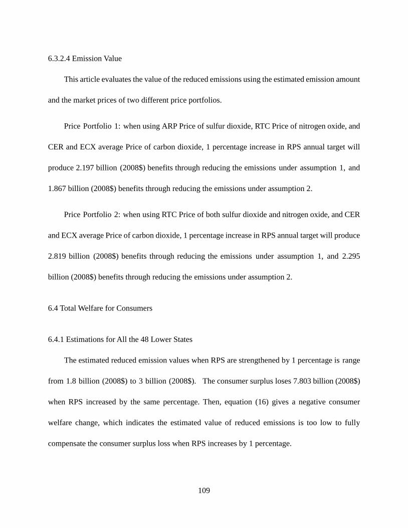
109

6.3.2.4 Emission Value

This article evaluates the value of the reduced emissions using the estimated emission amount

and the market prices of two different price portfolios.

Price Portfolio 1: when using ARP Price of sulfur dioxide, RTC Price of nitrogen oxide, and

CER and ECX average Price of carbon dioxide, 1 percentage increase in RPS annual target will

produce 2.197 billion (2008$) benefits through reducing the emissions under assumption 1, and

1.867 billion (2008$) benefits through reducing the emissions under assumption 2.

Price Portfolio 2: when using RTC Price of both sulfur dioxide and nitrogen oxide, and CER

and ECX average Price of carbon dioxide, 1 percentage increase in RPS annual target will produce

2.819 billion (2008$) benefits through reducing the emissions under assumption 1, and 2.295

billion (2008$) benefits through reducing the emissions under assumption 2.

6.4 Total Welfare for Consumers

6.4.1 Estimations for All the 48 Lower States

The estimated reduced emission values when RPS are strengthened by 1 percentage is range

from 1.8 billion (2008$) to 3 billion (2008$). The consumer surplus loses 7.803 billion (2008$)

when RPS increased by the same percentage. Then, equation (16) gives a negative consumer

welfare change, which indicates the estimated value of reduced emissions is too low to fully

compensate the consumer surplus loss when RPS increases by 1 percentage.

110

As is mentioned in Section 4, Table 6.9 includes consumer surplus loss, reduced amount and

estimated value of carbon dioxide, sulfur dioxide, and nitrogen oxide, consumer welfare, and

breakeven price for carbon dioxide when RPS annual target increased by 1 percentage under

different assumptions and price portfolios. This table also includes the estimations when

demand elasticity is assumed to be 0 using the same method in section 6.2 and section 6.3.

The table shows that all the estimates of total change in consumer‘s welfare are negative.

More specifically, 1 percentage increase in RPS annual target national wide can reduce consumer

welfare by 4.9 to 8 billion 2008 dollars according to different estimating approaches. Therefore,

strengthening RPS is no good to consumers even with an environmental concern.

Table 6.9 Consumer welfare change and breakeven price for carbon for all the states

Demand Elasticity= -0.558 Demand Elasticity= 0 Unit

assumption1 assumption2 assumption1 assumption2

△CS -7.803 -7.803 -7.861 -7.861 Billion 2008$

△CO2 38.627 34.597 8.764 4.674 Million tons

△SO2 0.204 0.140 0.043 -0.022 Million tons

△NOX 0.084 0.068 0.008 -0.008 Million tons

△Emissions1 -2.197 -1.867 -0.351 -0.016 Billion 2008$

△Benefit1 -5.606 -5.936 -7.510 -7.845 Billion 2008$

△Emissions2 -2.819 -2.295 -0.482 0.051 Billion 2008$

△Benefit2 -4.984 -5.508 -7.379 -7.912 Billion 2008$

$CO2 202.01 225.54 896.89 1681.64 2008$/Metric Ton

Notes: △Emissions1 and △Benefit1 uses the price in portfolio 1 including ARP Price of sulfur

dioxide, RTC Price of nitrogen oxide, and CER and ECX average price of carbon dioxide;

△Emissions2 and △Benefit2 uses the price in portfolio 2 including RTC Price of sulfur dioxide,

RTC Price of nitrogen oxide, and CER and ECX average price of carbon dioxide.

111

However, the value of reduced emissions is dependent on the price of the emission. If the

market prices of carbon dioxide, sulfur dioxide, and nitrogen oxide are underestimated, the real

effect of RPS on consumer welfare might be less negative or even positive.

One the other hand, the breakeven price for carbon dioxide is about 200 dollars in real 2008

price, which is much higher than the average of CER and ECX price for carbon dioxide ($27.288)

when demand elasticity is -0.558. When using zero demand elasticity, these breakeven prices

of carbon dioxide are even higher.

6.4.2 Estimations for Each of the Four Regions

Table 6.10 provides the related estimation results for each of the four regions including

original average electricity prices and sales, the consumer surplus change, reduced emission

amount and value, consumer welfare change, and breakeven price for carbon dioxide under

different assumptions of elasticity, renewable energy replaced sources, and price portfolios.

Table 6.10 shows that in the Northeast, 1 percentage increase in RPS can on average

decrease the consumer welfare by 0.2-0.3 billion dollars which implies RPS is more likely to be

inefficient policies in the Northeast. For the states in Midwest, 1 percentage increase in RPS

can on average increase the consumer welfare by 0.09-0.3 billion dollars which implies RPS is

an efficient policy in the Midwest. RPS is not that efficient in South since 1 percentage

increase in RPS can on average decrease the consumer welfare by 6-11 billion dollars. 1

percentage increase in RPS can on average increase the consumer welfare by 0.7-1.2 billion

dollars and hence an efficient policy in the states of West.

112

Table 6.10 Consumer welfare change and breakeven price for carbon for each region

Elasticity= -0.558 Elasticity= 0 Unit

assumption

1

assumption

2

assumption

1

assumption

2

Northeast

P 13.49 13.49 13.49 13.49 2008 cents/KWh

Q 0.457109 0.45710

9 0.45710

9 0.45710

9 MWh

△CS -0.294 -0.294 -0.294 -0.294 Billion 2008$

△CO2 0.764 0.764 0 0 Million tons

△SO2 0.004 0.004 0 0 Million tons

△NOX 0.002 0.002 0 0 Million tons

△Emissions1 -0.047 -0.047 0 0 Billion 2008$

△Benefit1 -0.247 -0.247 -0.294 -0.294 Billion 2008$

△Emissions2 -0.060 -0.060 0 0 Billion 2008$

△Benefit2 -0.234 -0.234 -0.294 -0.294 Billion 2008$

$CO2 384.61 384.61 -- -- 2008$/Metric Ton

Midwest

P 8.15 8.15 8.15 8.15 2008 cents/KWh

Q 0.780109 0.78010

9 0.78010

9 0.78010

9 MWh

△CS 0 0 0 0 Billion 2008$

△CO2 -5.118 -2.730 -5.118 -2.730 Million tons

△SO2 -0.025 -0.013 -0.025 -0.013 Million tons

△NOX -0.004 -0.005 -0.004 -0.005 Million tons

△Emissions1 -0.205 -0.009 -0.205 -0.009 Billion 2008$

△Benefit1 0.205 0.009 0.205 0.009 Billion 2008$

△Emissions2 -0.281 -0.009 -0.281 -0.009 Billion 2008$

△Benefit2 0.281 0.009 0.281 0.009 Billion 2008$

$CO2 -- -- -- -- 2008$/Metric Ton

South

P 8.26 8.26 8.26 8.26 2008 cents/KWh

Q 1.421109 1.42110

9 1.42110

9 1.42110

9 MWh

113

Table 6.10 (cont‘d)

△CS -9.987 -9.987 -10.236 -10.236 Billion 2008$

△CO2 43.412 43.412 0 0 Million tons

△SO2 0.234 0.234 0 0 Million tons

△NOX 0.111 0.111 0 0 Million tons

△Emissions1 -2.680 -2.680 0 0 Billion 2008$

△Benefit1 -7.307 -7.307 -10.236 -10.236 Billion 2008$

△Emissions2 -3.394 -3.394 0 0 Billion 2008$

△Benefit2 -6.593 -6.593 -10.236 -10.236 Billion 2008$

$CO2 230.05 230.05 -- -- 2008$/Metric Ton

West

P 8.12 8.12 8.12 8.12 2008 cents/KWh

Q 0.589109 0.58910

9 0.58910

9 0.58910

9 MWh

△CS 1.066 1.066 1.059 1.059 Billion 2008$

△CO2 -3.012 -3.739 1.539 0.821 Million tons

△SO2 -0.017 -0.028 0.008 -0.004 Million tons

△NOX -0.010 -0.013 0.001 -0.001 Million tons

△Emissions1 0.220 0.279 -0.062 -0.003 Billion 2008$

△Benefit1 0.846 0.787 1.121 1.062 Billion 2008$

△Emissions2 0.272 0.366 -0.085 0.009 Billion 2008$

△Benefit2 0.794 0.700 1.144 1.050 Billion 2008$

$CO2 353.88 285.07 -- -- 2008$/Metric Ton

To sum up, although RPS on average is not that efficient with emission concern for all the

48 lower states, the conclusion is different when doing regional level analysis. Table 6.10

shows that RPS is efficient in Midwest and in West but is not likely to be efficient in Northeast

and in South with emission concern. These findings are similar to the earlier prediction in

section 2.5.1 which implies RPS policies functioned well in Midwest and West while Northeast

and South are still struggling in how to make the policies on the track.

114

CHAPTER 7: CONCLUSION

Existing research on the effect of RPS policies in the United States assumes states have the

same trends of outcomes in absence of RPS, which is a hypothesis that is unlikely to hold in the

real world. What‘s more, no research estimates whether the value of reduced emissions from RPS

could compensate the negative effect of price increases, which might lead to positive consumer

welfare when enacts or strengthens RPS.

This article first uses Least Square Dummy Variable (LSDV) model to predict the effects of

RPS on renewable energy share in capacity, renewable energy share in generation, and price of

electricity. Then the basic model is advanced to control the effect of other RPS features and

other renewable energy policies, the concerns of partial effect of RPS, different trends of

outcomes in absence of RPS, and solve the serial correlation problem. The results imply RPS on

average are effective policies by estimating both significantly positive coefficients of RPS annual

target on renewable energy share in capacity and in generation but are not likely to be efficient

policies since RPS would significantly increase the electricity price, which makes for a serious

consumer surplus loss. Moreover, even with an emission concern, RPS still decrease total

welfare for consumers since the positive benefit on saving emissions cannot fully compensate the

consumer surplus loss in the electricity market if using the current market prices of carbon and

other emissions. But this conclusion might change if different per unit value of emissions is

applied. If the market prices used in this article underestimate the value of emissions to

consumers, it is still possible for RPS on average to be efficient policies with environmental

115

concern. The breakeven price for carbon dioxide is much higher than the market price, which

also means the cost of reducing the emission using this policy is too high. Finally, the regional

level analysis shows that RPS is efficient in Midwest and West but is not likely to be efficient in

Northeast and South with emission concern.

However, there is still point for further exploration especially the analysis and evaluation of

the emission value. This article uses the market trading price to evaluate the monetary value,

which always underestimates the emission value. The unit trading prices for CO2 in this article is

the price in European market rather than U.S. market. What‘s more, they are the prices for future

contracts and there is a gap between current price and futures even this article uses the nearest

contract prices. Even if the unit price this paper estimated is close to the real price, the current

price could be underestimated since there are other kinds of emissions reduced or increased due to

RPS that this article overlooked. Future studies could also estimate the emission value by

willingness to pay (WTP) approach, pollution capture cost approach or pollution damage

approach.

Moreover, there are other benefits if more renewable energy can substitute fossil fuels

which this paper doesn‘t take into account. For example, the reduced mercury emissions and

their effects on human health are also the benefit from RPS when using less coal. Even if we

consider all the costs and benefits of RPS and find they can increase consumer‘s welfare, it is

still hard to predict that RPS are the best renewable energy policies since they might not as

efficient as other policies.

116

APPENDIX

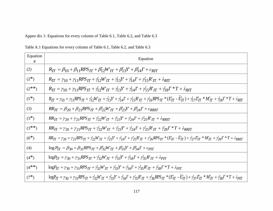
117

Appen dix 1: Equations for every column of Table 6.1, Table 6.2, and Table 6.3

Table A.1 Equations for every column of Table 6.1, Table 6.2, and Table 6.3

Equation

# Equation

(2)

(2*)

(2**)

(5*)

(3)

(3*)

(3**)

(6*)

(4)

(4*)

(4**)

(7*)

RITITITIT εI'Y'W'RPSR 1413121110

RITITITITIT λR'I'γY'γW'γRPSR 151413121110

RITITITITIT λTIγR'I'γY'γW'γRPSR *18151413121110

RITITITITITITITITITIT λTIγMZγEERPSR'I'γY'γW'γRPSR **)-(* 181716151413121110

RRITITITIT εI'Y'W'RPSRR 2423222120

RRITITITITIT λR'I'γY'γW'γRPSRR 252423222120

RRITITITITIT λTIγR'I'γY'γW'γRPSRR *28252423222120

RRITITITITITITITITITIT λTIγMZγEERPSR'I'γY'γW'γRPSRR **)-(* 282726252423222120

PITITITIT εI'Y'W'RPSP 3433323130log

PITITITITIT λR'I'γY'γW'γRPSP 353433323130log

PITITITITIT λTIγR'I'γY'γW'γRPSP *log 38353433323130

PITITITITITITITITITIT λTIγMZγEERPSR'I'γY'γW'γRPSP **)-(*log 383736353433323130

118

Appendix 2: Testing for Serial Correlation of Equation (2) in Appendix 1

Step One: Run the OLS regression for equation (2) and obtain the OLS residuals.

Step Two: Scatter graph reflects the relation between residuals and their lagged values in Figure

A.1.

Figure A.1 The relation between residuals and their lagged values in equation (2)

Step Three: Run the OLS regression of residuals on their lagged values, obtain the coefficient of

lagged residual and its t-value= 34.48 (p-value=0.000).

Conclusion: Serial Correlation is a problem in equation (2).

119

Appendix 3: Testing for Serial Correlation of Equation (2*) in Appendix 1

Step One: Run the OLS regression for equation (2*) and obtain the OLS residuals.

Step Two: Scatter graph reflects the relation between residuals and their lagged values in Figure

A.2.

Figure A.2 The relation between residuals and their lagged values in equation (2*)

Step Three: Run the OLS regression of residuals on their lagged values, obtain the coefficient of

lagged residual and its t-value= 26.65 (p-value=0.000).

Conclusion: Serial Correlation is a problem in equation (2*).

120

Appendix 4: Testing for Serial Correlation of Equation (2**) in Appendix 1

Step One: Run the OLS regression for equation (2**) and obtain the OLS residuals.

Step Two: Scatter graph reflects the relation between residuals and their lagged values in Figure

A.3.

Figure A.3 The relation between residuals and their lagged values in equation (2**)

Step Three: Run the OLS regression of residuals on their lagged values, obtain the coefficient of

lagged residual and its t-value= 17.57 (p-value=0.000).

Conclusion: Serial Correlation is a problem in equation (2**).

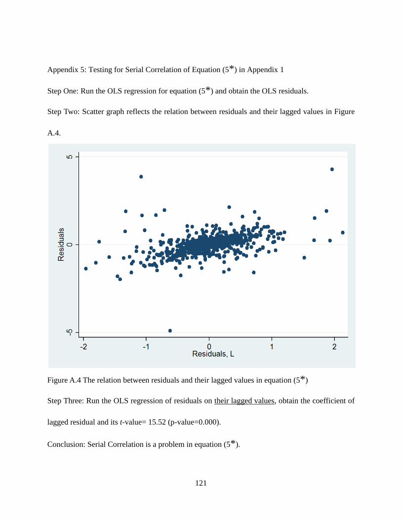
121

Appendix 5: Testing for Serial Correlation of Equation (5*) in Appendix 1

Step One: Run the OLS regression for equation (5*) and obtain the OLS residuals.

Step Two: Scatter graph reflects the relation between residuals and their lagged values in Figure

A.4.

Figure A.4 The relation between residuals and their lagged values in equation (5*)

Step Three: Run the OLS regression of residuals on their lagged values, obtain the coefficient of

lagged residual and its t-value= 15.52 (p-value=0.000).

Conclusion: Serial Correlation is a problem in equation (5*).

122

Appendix 6: Testing for Serial Correlation of Equation (3) in Appendix 1

Step One: Run the OLS regression for equation (3) and obtain the OLS residuals.

Step Two: Scatter graph reflects the relation between residuals and their lagged values in Figure

A.5.

Figure A.5 The relation between residuals and their lagged values in equation (3)

Step Three: Run the OLS regression of residuals on their lagged values, obtain the coefficient of

lagged residual and its t-value= 21.50 (p-value=0.000).

Conclusion: Serial Correlation is a problem in equation (3).

123

Appendix 7: Testing for Serial Correlation of Equation (3*) in Appendix 1

Step One: Run the OLS regression for equation (3*) and obtain the OLS residuals.

Step Two: Scatter graph reflects the relation between residuals and their lagged values in Figure

A.6.

Figure A.6 The relation between residuals and their lagged values in equation (3*)

Step Three: Run the OLS regression of residuals on their lagged values, obtain the coefficient of

lagged residual and its t-value= 18.40 (p-value=0.000).

Conclusion: Serial Correlation is a problem in equation (3*).

124

Appendix 8: Testing for Serial Correlation of Equation (3**) in Appendix 1

Step One: Run the OLS regression for equation (3**) and obtain the OLS residuals.

Step Two: Scatter graph reflects the relation between residuals and their lagged values in Figure

A.7.

Figure A.7 The relation between residuals and their lagged values in equation (3**)

Step Three: Run the OLS regression of residuals on their lagged values, obtain the coefficient of

lagged residual and its t-value= 10.54 (p-value=0.000).

Conclusion: Serial Correlation is a problem in equation (3**).

125

Appendix 9: Testing for Serial Correlation of Equation (6*) in Appendix 1

Step One: Run the OLS regression for equation (6*) and obtain the OLS residuals.

Step Two: Scatter graph reflects the relation between residuals and their lagged values in Figure

A.8.

Figure A.8 The relation between residuals and their lagged values in equation (6*)

Step Three: Run the OLS regression of residuals on their lagged values, obtain the coefficient of

lagged residual and its t-value= 2.95 (p-value=0.003).

Conclusion: Serial Correlation is a problem in equation (6*).

126

Appendix 10: Testing for Serial Correlation of Equation (4) in Appendix 1

Step One: Run the OLS regression for equation (4) and obtain the OLS residuals.

Step Two: Scatter graph reflects the relation between residuals and their lagged values in Figure

A.9.

Figure A.9 The relation between residuals and their lagged values in equation (4)

Step Three: Run the OLS regression of residuals on their lagged values, obtain the coefficient of

lagged residual and its t-value= 39.97 (p-value=0.000).

Conclusion: Serial Correlation is a problem in equation (4).

127

Appendix 11: Testing for Serial Correlation of Equation (4*) in Appendix 1

Step One: Run the OLS regression for equation (4*) and obtain the OLS residuals.

Step Two: Scatter graph reflects the relation between residuals and their lagged values in Figure

A.10.

Figure A.10 The relation between residuals and their lagged values in equation (4*)

Step Three: Run the OLS regression of residuals on their lagged values, obtain the coefficient of

lagged residual and its t-value= 37.43 (p-value=0.000).

Conclusion: Serial Correlation is a problem in equation (4*).

128

Appendix 12: Testing for Serial Correlation of Equation (4**) in Appendix 1

Step One: Run the OLS regression for equation (4**) and obtain the OLS residuals.

Step Two: Scatter graph reflects the relation between residuals and their lagged values in Figure

A.11.

Figure A.11 The relation between residuals and their lagged values in equation (4**)

Step Three: Run the OLS regression of residuals on their lagged values, obtain the coefficient of

lagged residual and its t-value= 17.19 (p-value=0.000).

Conclusion: Serial Correlation is a problem in equation (4**)

129

Appendix 13 Testing for Serial Correlation of Equation (7*) in Advanced Model

Step One: Run the OLS regression for equation (7*) and obtain the OLS residuals.

Step Two: Scatter graph reflects the relation between residuals and their lagged values in Figure

A.12.

Figure A.12 The relation between residuals and their lagged values in equation (7*)

Step Three: Run the OLS regression of residuals on their lagged values, obtain the coefficient of

lagged residual and its t-value= 13.64 (p-value=0.000).

Conclusion: Serial Correlation is a problem in equation (7*).

130

BIBLIOGRAPHY

131

Arthur, W. (1990). Positive Feedbacks in the Economy. Scientific American, February, 92–99.

Arthur, W. (1994). Path Dependence, Self-Reinforcement, and Human Learning. Increasing

Returns and Path Dependence in the Economy, Ann Arbor: University of Michigan Press,

133–58.

Bernow, S., Dougherty, W., & Duckworth, M. (1997). Quantifying the Impacts of a National,

Tradable Renewables Portfolio Standard. The Electricity Journal, 10 (4), 42-52

Burns, D. (2010). National Acid Precipitation Assessment Program Report to Congress: An

Integrated Assessment. Annual RECLAIM Audit Report for 2008 Compliance Year.

Carley, S. (2009). State Renewable Energy Electricity Policies: An Empirical Evaluation of

Effectiveness. Energy Policy 37(8), 3071-3081

Chen, C., Wider, R., Mills, A., & Bolinger, M. (2009). Weighing the Costs and Benefits of State

Renewable Portfolio Standards in the United States: A comparative Analysis of State-level

Policy Impact Projection, Renewable and Sustainable. Energy Reviews, 13, 552-566

Elliot, R., Anna M., Steven N., & Elizabeth B. (2003). Natural Gas Price Effects of Energy

Efficiency and Renewable Energy Practices and Policies. Report E032. Washington:

American Council for an Energy-Efficient Economy.

Elliott, D.L., Wendell, L.L., & Gower, G.L. (1991). An Assessment of the Available Windy Land

Area and Wind Energy Potential in the Contiguous United States. Technical Report, 08

Espey, S. (2001). Renewable Portfolio Standard: a Means for Trade with Electricity from

Renewable Energy Sources. Energy Policy 29 (7), 557–566.

Fischer, C. (2006). How Can Renewable Portfolio Standards Lower Electricity Prices? RFF

Discussion Papers 06-20.

Gouchoe, S., Everette, V., & Haynes, R. (2002). Case Studies on the Effectiveness of State

financial incentives for renewable energy. NREL/SR-620-32819, National Renewable

Energy Laboratory, Raleigh, NC.

Hindman, D. (2009). Mass Media Flow and Differential Distribution of Politically Disputed

Beliefs: The Belief Gap Hypothesis. Journalism and Mass Communication Quarterly 86,

790-808.

132

Ho, D., Kosuke, I., Gary, K., & Elizabeth, S. (2007). Matching as Nonparametric Preprocessing

for Reducing Model Dependence in Parametric Causal Inference. Political Analysis, 15 (3),

199-236.

Hodgson, G. (1998). The Approach of Institutional Economics. Journal of Economic Literature,

36(March), 166–192.

Iyengar, S, & Kyu, H. (2009). Red Media, Blue Media. Journal of Communication 59, 19-39.

Johnson, E. (2010). The Price Elasticity of Supply of Renewable Electricity Generation:

Evidence from State Renewable Portfolio Standards. Dissertation and Job Market Paper.

from http://www-personal.umich.edu/~johnsoep/docs/epjohnson_rps.pdf

Kneifel, J. (2008). Effects of State Government Policies on Electricity Capacity from

Non-Hydropower Renewable Sources. Mimeo, University of Florida.

Lahsen, M. (2005). Technocracy, Democracy, and U. S. Climate Politics. Science, Technology &

Human Values 30, 137-169.

Lahsen, M. (2008). Experiences of Modernity in the Greenhouse: A Cultural Analysis of a

Physicist ‗Trio‘ Supporting the Backlash against Global Warming. Global Environmental

Change, 18, 204-19.

Langniss, O., & Wiser, R. (2003). The Renewable Portfolio Standard in Texas: An Early

Assessment. Energy Policy 31 (6), 527–535.

Layzer, J. (2007). Deep Freeze: How Business Has Shaped the Global Warming Debate in

Congress. Business and Environmental Policy, Cambridge, MA: MIT Press.

Lyon, T., & Yin, H. (2007). Why Do States Adopt Renewable Portfolio Standards? An Empirical

Investigation. Available at SSRN: http://ssrn.com/abstract=1025513

McCright, A., & Riley, D. (2000). Challenging Global Warming as a Social Problem. Social

Problems, 47, 499-522.

McCright, A., & Riley, D. (2003). Defeating Kyoto: The Conservative Movement‘s Impact on

U.S. Climate Change Policy. Social Problems, 50(3), 348-73.

Mercuro, N., & Steven, M. (2006). Economics and the Law: From Posner to Post-Modernism

133

and Beyond. Second Edition. Princeton, NJ: Princeton University Press.

Nielsen, R., & Sheffield, J. (2009). Matching with Time-Series Cross-Sectional Data.

Conference on Political Methodology. from

http://polmeth.wustl.edu/conferences/methods2009/resources/papers/Nielsen-PanelMatch

ing2009-poster.pdf

Oreskes, N., & Erik, C. (2010). Merchants of Doubt: How a Handful of Scientists Obscured the

Truth on Issues from to Bacco Smoke to Global Warming. New York: Bloomsbury Press.

Palmer, K., & Dallas, B. (2005). Cost-Effectiveness of Renewable Electricity Policies. Energy

Economics, 27(6), 873-894.

Rabe, G. (2006). Race to the Top: The Expanding Role of U.S. State Renewable Portfolio

Standards. Prepared for the Pew Center on Global Climate Change.

Rader, N., & Norgaard, R. (1996). Efficiency and Sustainability in Restructured Electricity

Markets: The Renewables Portfolio Standard. The Electricity Journal, July 1996. 37-49

Schmid, A. A. (1987). Property, Power and Public Choice: An Inquiry into Law and Economics.

New York, Praeger.

Schmid, A. A. (2001). Institutional and Behavioral Economics. East Lansing, Walbridge Press.

Schmid, A. A. (2004). Conflict and Cooperation: Institutional and Behavioral Economics.

Malden, MA: Blackwell.

U.S. National Academies of Science Panel on Advancing the Science of Climate Change. (2010).

Advancing the Science of Climate Change. Washington, D.C., National Academies Press.

U.S. National Academies of Science Panel on Limiting the Magnitude of Future Climate Change.

(2010). Limiting the Magnitude of Future Climate Change. Washington, D.C., National

Academies Press.

Wiser, R., & Barbose, G. (2008). Renewable Portfolio Standards in United States: A Status

Report with Data through 2007. Lawrence Berkeley National Laboratory.

Wiser, R., Namovicz, C., Gielecki, M., & Smith, R. (2007). The Experience with Renewable

Portfolio Standards in the United States. The Electricity Journal, 20 (4).

134

Yin, H., & Powers, N. (2010). Do state renewable portfolio standards promote in-state renewable

generation ? Energy Policy, 38(2), 1140-114.