Embed Size (px)
Citation preview

THE I-70 GREENFIELD REST AREA WETLAND PROJECTS: REPORT ON INTERIM RESULTS
SPR-2456 Hydrology of Natural and Constructed Wetlands SPR-2455 Constructed Wetlands for INDOT Rest Stop Wastewater Treatment: Proof of
Concept Research SPR-2487 Constructed Wetland Systems for Wastewater Management
by
R. Sultana S.-C. Kao
T. Konopka S. Tripathi T. P. Chan
T. J. Cooper J. E. Alleman
R. S. Govindaraju
January, 2007
Purdue University West Lafayette, Indiana


i
ACKNOWLEDGEMENTS Gratitude is expressed to the Joint Transportation Research Program (JTRP) at Purdue University for providing the funds to conduct the research described here. Numerous people have been involved with this project in various capacities, and they have been listed below. Their help in this effort is acknowledged. SAC – Members for SPR-2487, 2455, and 2456
Fike Abasi INDOT Design Division Tony DeSimone FHWA Indiana Division Merril Dougherty INDOT Design Division Tom Duncan INDOT Pre-Engineering and Environment Division Clyde Mason INDOT Greenfield District Steve McAvoy INDOT Operations Support Division Joyce Newland FHWA Indiana Division Barry Partridge INDOT Office of Research and Development Steve Sperry INDOT Environment, Planning, and Engineering DivisionJerry Unterreiner INDOT Pre-Engineering and Environment Division Tom Vanderpool INDOT Greenfield District JoAnn Wooldridge INDOT Greenfield District
Outside Members Andrew Bender J. F. New T. Blahnik J. F. New Ed. Miller Indiana Department of Health Matt Moore RQAW Brian Morgan Heritage Industries Steve Land INDOT/PS David Latka J. F. New
Purdue Team Students T. P. Chan, S.-C. Kao, S. Khanal, T. Konopka,
N. Shah, S. Sharma, R. Sultana, S. Tripathi Laboratory and Field Research Coordinator
T. J. Cooper
Faculty J. E. Alleman, R. S. Govindaraju, R. Wukasch

ii
DISCLAIMER While this study has been funded by Joint Transportation Research Program (JTRP) at Purdue University, this report has not undergone a review by either the JTRP board or the Indiana Department of Transportation (INDOT). Hence, conclusions presented are only those of the authors. Use of trade names for various products in this report is for information purposes only, and no official endorsement is implied.

iii
TABLE OF CONTENTS
Page Acknowledgements…………………………………………………………………………i Disclaimer………………………………………………………………………………….ii Table of contents…………………………………………………………………………..iii Summary…………………………………………………………………………………...v Chapter 1. Introduction……………………………………………………………..............1
1.1. Background and motivation…………………………………………………………1 1.2. Previous work……………………………………………………………………….4 1.3. Scope of this report………………………………………………………………….8
Chapter 2. Basic concepts and definitions in wetlands……………………………………..9
2.1. Definition and classification of wetlands……………………………………………9 2.2. Hydrologic factors related to wetlands…………………………………………….12 2.3. Environmental factors in wetland treatment……………………………………….15
Chapter 3. Greenfield wetland system…………………………………………………….19
3.1. Project background………………………………………………………………...19 3.2. Treatment system design…………………………………………………………..21
3.2.1. Septic tanks……………………………………………………………………22 3.2.2. Subsurface wetland system……………………………………………………23 3.2.3. Wetland media………………………………………………………………...25 3.2.4. Dosing tanks…………………………………………………………………..25 3.2.5. Biofield………………………………………………………………………..27 3.2.6. Wetland plants………………………………………………………………...28
3.3. Wetland operation scheme…………………………………………………………29 3.4. Instrumentation at the Greenfield site……………………………………………...31
3.4.1. Flow measurements…………………………………………………………...31 3.4.2. Water quality sampling………………………………………………………..34 3.4.3. Weather station………………………………………………………………..36
3.5. Description of the data……………………………………………………………38 3.5.1. Flow meter data…………………………………………………………..........40 3.5.2. Magnetic flow meter data……………………………………………………..41 3.5.3. Weather station data…………………………………………………………...44

iv
Chapter 4. Hydrologic performance………………………………………………………45 4.1. Introduction………………………………………………………………………..45 4.2. Model description………………………………………………………………….45 4.3. Model calibration…………………………………………………………………..48 4.4. Model validation…………………………………………………………………...55 4.5. Limitations of the hydrologic model……………………………………………….59
Chapter 5. Wetland plants and treatment performance……………………………………61
5.1. Introduction………………………………………………………………………..61 5.2. Wetland plants……………………………………………………………………62 5.3. Visual trends in plant growth at Greenfield………………………………………66 5.4. Treatment performance…………………………………………………………….67
Chapter 6. Recommendations and future work……………………………………………71
6.1. Conclusions………………………………………………………………………..71 6.2. Recommendations…………………………………………………………………72 6.3. Future work……………………………………………………………………….73
References………………………………………………………………………………...74
Appendix A. Time line for wetland project……………………………………………….78

v
SUMMARY A constructed wetland system was built at the Greenfiield rest stop due east of Indianapolis on interstate highway I-70. Because of the high strength of wastewater generated at the rest stop, a wetland system was built with two parallel wetlands cells followed by a third wetland cell in series. Apart from the cells, the wetland complex contains one surge tank, two septic tanks, four lift stations, and two actuator chamber. The parallel wetland cells operate on alternate fill-and-drain cycle along with recirculation, while the third wetland operates like a conventional plug-flow reactor. The system was instrumented to evaluate the performance of the various components of the system. This report describes the wetland complex, data, initial modeling and analysis. It provides an assessment of the progress into the project. A hydraulic model was developed for the wetland complex. The logic behind the operations of the lift stations, wetland cells with the fill-and-draw scheme, and the actuator switches were incorporated in the model. Since, there was difficulty in obtaining good quality data for calibration and validation over sustained time periods, the model must primarily be viewed as a starting point. This model can be further improved by using more reliable sets of data. Model results show that hydraulic retention time (HRT) of parallel wetlands and polishing wetland are about 6 days, and 1 day, respectively. Data collected so far seem to indicate that health of plants in the wetland system is a key factor for achieving good treatment. Poor percentage removals were found to occur when plants were not functioning well. Based on the operation thus far (July, 2006), the wetland complex has not been able to achieve treatment levels that would allow for either surface or subsurface disposal into the environment. When the plants are healthy and the wetlands are functioning properly, significant ammonia, TSS, and BOD removals do occur, but we hypothesize that enough oxygen is not available for treating the waste despite the fill-and-draw procedure. The lessons learned so far are: (1) Maintenance of the wetland facility is a key factor for good performance. (2) The draw and fill timing needs to be monitored carefully. (3) Draining of septic tanks is required at about every 3 months.

vi
(4) Accurate recording of flow data will be needed. In future, following topics will be addressed: (1) A cost comparison (at least qualitatively) to evaluate wetlands versus other treatment
options such as packaged plants. (2) Assessment of HRT on treatment with better data, surge tank, and SCADA system. (3) Estimation of mass reductions along with percentages to quantify wetland
performance.

1
CHAPTER 1
INTRODUCTION 1.1 BACKGROUND AND MOTIVATION Until the mid twentieth century, wastewater generated from industries and consolidated areas were dumped into nearby lakes, rivers, and other water bodies. As a result, these water bodies became highly polluted and posed a serious threat to public health and safety. Some water bodies, such as Cuyahoga River in Ohio were so polluted that they burst into flames (http://drake.marin.k12.ca.us/stuwork/rockwater/The%20Clean%20Water%20Act/History%20and%20stories.html). These incidents raised public awareness about water quality issues. To address these concerns, the Federal Water Pollution Control Act (FWCWA) was enacted in 1946, and is the first legislative effort to deal with water quality problems. The act was amended numerous times until it was recognized and expanded in 1972, and formed the basis for the current Clean Water Act (CWA). This act made it unlawful for any person or entity to discharge any pollutants from a point source into navigational waters without a permit. It is because of such legislation that industries and municipalities are required to treat their waste water before discharging into nearby waterways. Since then, waste water treatment plants have become a very important part of our efforts to preserve the environment, and to provide waters that we can use everyday for drinking, swimming, and fishing. Conventional treatment plants are known to expend a lot of energy. In United States, for small communities (less than 10,000 population), construction costs vary on an average between $10 and $15 billion nationwide (Hammer, 1997). Moreover, complete sewage treatment for all the residents in United States is unlikely, and in some cases undesirable because of geographic, economic and sustainability reasons (Crites and Tchobanoglous, 1998). These reasons apply more to developing countries, where financial constraints are greater due to increased costs incurred because of unreliability of operation and maintenance services. In developing countries, decentralized sanitation in the form of septic tanks is used in all rural areas and in many parts of urban areas as well. Even in developed countries, where provision of centralized sewage treatment exists, decentralized sanitation still plays an important role (Metcalf and Eddy, 1991). In United

2
States alone, more than 60 million people live in homes that are served by decentralized collection and treatment systems (Crites and Tchobanoglous, 1998). Moreover, because of reduction in funding for large sewage treatment systems, many small communities in United States have turned to onsite sewage treatment technologies. All these reasons underscore the need for a continual effort to identify and encourage technologies that provide effective, environmentally friendly, on-site treatment at low cost. One of the low-cost technologies is the use of wetlands for wastewater treatment. In recent times, wetlands have gained popularity over conventional treatment options for small communities, and for businesses located at decentralized locations. In the past, natural wetlands have received wastewater from many sources, but they have been recognized as a cost effective treatment system only relatively recently. In 1952, perhaps the first experiment to evaluate the possibilities of using wetland plants for wastewater treatment was conducted by the Max Planck Institute in Ploen, Germany. Then, more than 20 years later, the first operational full-scale constructed wetland for municipal sewage was built in Germany. In 1973, United States’ first engineered constructed wetland (CW) treatment pilot systems were constructed in Brookhaven National Laboratory near Brookhaven, NY. Since then CWs have been used as a cost effective alternative in treating domestic, industrial, and municipal wastewater and also for storm water management. The goal of CWs is to use the natural treatment mechanisms of wetlands to reduce downstream pollutant discharges. In wetlands, the physical, chemical, and biological processes required for treatment occur in a natural environment instead of synthetic reactor tanks, or basins with artificial chemicals, as in conventional treatment plants. Wetland systems are touted as being low-maintenance technologies, as opposed to conventional treatment plants that require skilled personnel to be present on site. As a result, natural wetlands are often used for treatment of wastewaters. Wetlands are also constructed at desired locations so as to mimic the treatment mechanisms existing in natural wetlands. Because of the effectiveness of the wetlands at low cost, many developing and developed countries over the last 10 to 15 years have chosen to use them for wastewater treatment for small communities. A wetland system in Tanzania has improved the influent wastewater quality by reducing nitrogen concentration by 70%, chemical oxygen demand by 90%, and almost 100% reduction of total coliform (Mbuligwe, 2005). The final effluent is being used for irrigation. In India, a wetland system that was constructed for a school has successfully reduced the ammonia (66-73%), phosphorus (23-48%), and

3
biological oxygen demand (78-91%) (Juwarkar et al., 1995). A number of studies in United States have also shown significant removal efficiency by the wetland system (Steer et al., 2005; Huang et al., 2000). Wetlands have been found suitable for tropical climates (Kantawanichkul et al., 1999), and many European countries have found that wetlands can perform reasonably even in cold climates (Maehlum and Stalnacke, 1999; Maehlum et al., 1995; Haberl et al., 1995). These systems use either single or multiple wetland cells for treatment. In multiple-cell systems, each cell might have different treatment objectives, but their combined effect can improve performance over a single- cell system. Success of wetlands in these and other past studies have prompted the Indiana Department of Transportation (INDOT) to investigate the use of wetlands for the treatment of wastewater generated from highway rest areas. Wastewater treatment from a highway rest area often has some unique characteristics which have long posed significant challenges for highway engineers. So, INDOT undertook a set of three individual “long-range” research projects under the “Wetlands focus area theme” of the “JTRP-INDOT Strategic Environment Focus Area”. The three projects were:
(1) Constructed wetlands (CW) for INDOT rest stop wastewater treatment. (2) CW systems for wastewater management. (3) Hydrology of natural and constructed wetlands.
All these projects were developed to facilitate a coordinated experimental evaluation of a full scale, proof-of-concept, constructed wetland of an INDOT rest stop. It was decided to build a new CW at the Greenfield rest stop due east of Indianapolis on I-70. This rest stop is fairly new and was designed by RQAW, Inc. The rest stop toilets have low-flow faucets, consequently generating high strength of wastewater that had to be pumped to the local treatment plant in Greenfield, IN, greater than 3 miles away. The constructed wetland was built with an aim to reduce the pollutant concentrations (mainly ammonia) so that the Greenfield municipal treatment facility would not need to bear this load. This is perhaps the first wetland system in United States that has a network of cells and treats wastewater from a highway rest area. INDOT wants to treat this wetland system as a test site. To evaluate the performance of different parts of the system, it has been instrumented for flow and water quality measurements. It was hoped that if this wetland was successful in meeting the regulations for various effluents, then the wetland will be used as “reference

4
wetland” for other rest areas in the state. Moreover, the experience gained at this site could be used for designing and building similar facilities at other sites. The purpose of this report is to provide an assessment of the progress thus far. 1.2 PREVIOUS WORK Constructed wetlands are of two types: subsurface flow constructed wetlands (SFCW) are designed exclusively for stormwater/wastewater treatment, while the free water surface wetlands (FWS) are commonly used for wildlife habitat and public recreational opportunities. The focus of this section is on SFCW because the Greenfield rest area uses a network of SFCWs. When a SFCW is used for stormwater treatment, the main objective is to remove total suspended solids (TSS) and heavy metals from runoff. But, SFCWs for wastewater treatment are expected to remove not only TSS and heavy metals, but also fecal coliforms, biochemical oxygen demand (BOD), chemical oxygen demand (COD), ammonia- nitrogen (NH3-N), and phosphorus (P) from wastewater. The designs of SFCWs are dictated by treatment objectives. Wetland performance depends on factors like:
- Wetland soil type, soil chemistry, and the kind of reactions that occur between the soils and the contaminants.
- Operating water depths, hydraulic loading rate, physical configuration of the wetland systems (Wieder et al., 1989).
- Contaminant uptake by vegetation (Watson and Hobson, 1989). - Hydrology and hydraulic design of the wetland (Kadlec, 1989; Owen, 1995; Persson and Wittgren, 2003).
Wetland systems are usually designed to provide primary treatment to the wastewater stream through a single or multiple septic tanks or facultative ponds before the wastewater flows into the wetland systems. It has been found that wetlands are efficient in removing fecal colliforms, BOD, COD, and TSS (all around 90%) although showing low efficiency in NH3-N (50-60%), and P (25-45%) removal (Juwarkar et al., 1995; Kantawanichkul et al., 1999; Platzer, 1999; Manios et al., 2003; Mbuligwe, 2005; Steer et al., 2005). However, high removal rate of BOD, COD is influenced by organic loading

5
rate (Persson and Wittgren, 2003). With high loading rate, removal efficiency of BOD, and COD can even decrease to 70%. Unfortunately, not all studies cite influent organic loading rates. Another important factor influencing removal rate is how the influent is fed into the wetland system by vertical flow or by horizontal flow. Systems with horizontal flow can remove BOD, COD, TSS, and fecal coliforms significantly, but tend to have very low NH3-N, P removal efficiency (Juwarkar et al., 1995; Mbuligwe, 2005; Steer et al., 2005). On the other hand, systems with vertical flow show high percentage of removal of NH3-N (Kantawanichkul, 1999). Studies have shown that a combination of both types of flow is better than only vertical flow or only horizontal flow systems (White, 1995; Maehlum et al., 1999; Platzer, 1999). This is because vertical flow systems provide aerobic environments to enhance nitrification and horizontal flow systems provide anaerobic subsurface flow environments for denitrification, and nitrogen removal requires both the processes. Pollutant removal efficiency is also influenced by the type of media used in the cell. Studies show that gravel beds with gravel sizes between 5-30 mm are better to allow for roots to develop and offer sufficient surface area for physical, chemical, and microbiological processes to occur unhindered (Manios et al., 2003). Most studies showed that plants played little or no role in treatment. However, one study found that planted wetland cells had much greater removal efficiency than unplanted wetland cells (Juwarkar et al., 1995). In some systems, a portion of the effluent is recycled back to improve treatment efficiency. The percentage of effluent recycled back is also an important factor. White (1995) had studied 3 wetland systems where 0%, 100%, or 200% effluent was recycled back as the influent, and found that the system recycling 100% effluent was more effective than systems recycling 0%, or 200% effluent. Wetland modeling efforts have ranged from attempts to describe very specific wetland processes to detailed models of wetland hydrology and nutrient cycles. Mitsch (1983) classified wetland models into seven categories: (1) energy/nutrient models; (2) hydrological models; (3) spatial ecosystem models; (4) tree growth models; (5) process models; (6) causal models; and (7) regional energy models. Again, models that are developed for wetlands are very site and application specific, and models results have not been easily transferable.

6
Almost all models treat wetlands as an ideal plug-flow reactor or a continuously stirred tank reactor (CSTR), with the former being more popularly used. The models assuming ideal plug-flow behavior tend to overestimate the removal efficiency (Dahab et al., 2001). Assumption of ideal plug flow behavior implies that all the particles in the liquid advance in the tank or reactor with equal velocity while in case of CSTR all the particles in the liquid are perfectly mixed, and inflow and outflow rates are same. The CSTR models show some degree of success (Kadlec, 1994; Kadlec and Knight 1996). However, wetland hydraulics is neither completely plug-flow nor CSTR. In reality, a wetland behaves somewhere between the two extremes. So, it is better to model wetlands as a combination of plug-flow reactor along with a number of continuously stirred tank reactors (Kadlec and Knight, 1996). Wynn and Liehr (2001) developed a mechanistic model that simulates hydraulic behavior of a wetland by CSTR approach. They calibrated the model using the data from a constructed wetland in Maryland. The model requires estimation of 15 initial conditions and knowledge of 42 parameters which is not a convenient task. Recently, Martinez and Wise (2003) used United States Geological Survey’s (USGS) one dimensional transient inflow and outflow model (OTIS) in 17 Orlando Easterly Wetland cells to analyze wetland hydraulics. The transient model combines plug flow with dispersion equations, and the model results were found to agree well with field data. The model was calibrated first using tracer test results. Tracer test is a simple and often used tool for hydraulic analysis. Usually, a tracer is injected at the inlet of the system and collected at the outlet. The Greenfield wetland system is a rather complex network of 3 wetland cells with recirculation, and includes septic tanks and lift stations. Fig 1.1 shows a site plain view of this complex. A detailed hydraulic analysis of this system would be very complicated. So, a simple tracer test may not suffice to evaluate the performance of all units of the system. This hydraulic complexity necessitated the development of a separate model for the Greenfield wetland system.

7
Figure 1.1 – Plan view of the wetland complex at the Greenfield Rest Stop on I-70

8
1.3 SCOPE OF THE REPORT In Chapter 2, wetland types and factors that need consideration for wetland design are briefly discussed. Chapter 3 provides a detailed description of the Greenfield wetland system. Chapter 4 describes the hydrologic model of the Greenfield wetland system, and focuses on how the model was built and presents results for model corroboration. Chapter 5 deals with wetland plants and evaluation of the wetlands from a treatment perspective. Chapter 6 describes the lessons learned so far, and what future activities are planed for this project.

9
CHAPTER 2
BASIC CONCEPTS AND DEFINITIONS IN WETLANDS
2.1 DEFINITION AND CLASSIFICATION OF WETLANDS Wetlands are also known as slough, brackish marsh, freshwater swamp, and ponds (Hammer and Bastian, 1989; Persson and Wittgren, 2003). Wetlands can be defined as vegetated land areas that are wet during part or all the year, with the water surface in the wetlands near to the ground keeping the soil saturated (US EPA, 1988; Kadlec and Knight, 1996). The committee on Wetland Characterization defined wetlands as:
“.. an ecosystem that depends on a constant or recurrent, shallow inundation or saturation at or near the surface of the substrate. The minimum essential characteristics of a wetland are recurrent, sustained inundation or saturation at or near the surface and the presence of physical, chemical, and biological features…. Common diagnostic features of wetlands are hydric soils and hydrophytic vegetation except where specific physicochemical, biotic, or anthropogenic factors have removed them or prevented their development.”
Wetland soils lack oxygen as a result of being saturated for extended periods. For annual vegetation production, the soils typically contain a high proportion of organic matter. Because of anaerobic conditions and presence of thick litter layer, wetland soils provide an environment where several chemical and microbial processes can thrive. Wetlands provide ideal conditions for a wide variety of microorganisms which are the “workhorses” in the wetland treatment processes. Hammer (1997) classified wetlands into five different groups based on various criteria. These are:
Natural WetlandsThese are the wetlands where the substratum is periodically flooded throughout the
year. Some wetlands support a variety of plants and animal species. They are considered waters of the U.S. and are subject to discharge regulations.

10
Constructed WetlandsThese wetlands are created from non-wetland sites, with the primary purpose
commonly being wastewater treatment. Constructed wetlands treat wastewater by chemical, biological, and physical processes that are typical of natural wetlands. Physical entrapment and sedimentation of wastewater solids are also key processes aiding the removal of pollutants. Constructed wetlands themselves are not considered waters of the U.S. Discharges from constructed wetlands into the waters of the U.S. are regulated, and must adhere to NPDES permits.
Created wetlands These are wetlands created to replace destroyed habitat on site or elsewhere. They
are considered waters of the U.S., and are subject to discharge requirements. Restored Wetlands Several areas existed as natural wetland systems in the past, but were altered in such
a manner as to eliminate typical flora/fauna species. Subsequently, original conditions were reinstated in some instances creating conditions for natural flora/fauna to return to the system. These are called as restored wetlands, and are waters of the U.S. that are subject to discharge regulation.
Floating Aquatic Systems These are systems that support fully floating vegetation such as water hyacinth
(Eichhornia spp) and duckweed (Lemna spp). They are subject to NPDES permitting regulations. Constructed wetlands are further classified into two groups: free water surface systems (FWS), and subsurface flow constructed wetlands (SFCW). These are described briefly.
Free Water Surface (FWS) Systems FWS systems are designed as a basin to simulate natural wetlands. In this system,
water is generally introduced above the ground surface, is open to the atmosphere, and then it flows through the wetland. The depth of water in the wetlands varies from 6 to 12 inches. The wetlands are typically divided into cells by using earthen berms, concrete, or wood to ensure smooth flow and maximum contact between water and wetland plants. FWSs are frequently used to maximize wetland habitat values and reuse opportunities while improving water quality. Figure 2.1 shows a typical FWS system.

11
Figure 2.1 – Profile view of a free water surface wetland
(Source: http://www.extension.umn.edu/distribution/naturalresources/DD7671.html)
Subsurface Flow Constructed wetland systems (SFCW) SFCWs are usually shallow gravel beds where water passes horizontally below the
ground surface across the bed. Therefore odors, and other nuisance problems that are common in FWS wetlands are generally eliminated in SFCWs. Typically soil, sand, gravel, or crushed rocks are used to create this permeable medium that may be as much as 4 feet thick from the ground surface. The extensive root system growing in the gravel media provides a substrate for microbial communities responsible for pollutant reduction. Typically, these wetlands use impermeable liners to prevent groundwater contamination. SFCWs are designed and operated to improve water quality. Figure 2.2 shows a typical SFCW system.
Figure 2.2 – Profile view of Subsurface Flow system
(Source: http://www.extension.umn.edu/distribution/naturalresources/DD7671.html) It is believed that there are other benefits offered by SFCWs when compared to FWSs. Because of the porous media used in SFCWs, they offer more surface area for treatment

12
than FWS systems. As a result, treatment efficiency is higher. In addition, there is better thermal protection within SFCWs so that bacterial activity may continue at deeper locations of the wetland even during cold weather. 2.2 HYDROLOGIC FACTORS RELATED TO WETLANDS Important components of wetland hydrology are precipitation, infiltration, evapo- transpiration, water depth, and hydraulic loading rate. Kadlec and Knight (1996), Watson and Hobson (1989), Kadlec (1989), and Mitsch and Gosselink (1993) discussed wetland hydrology to varying degrees of detail. Some of the common terms and concepts associated with wetland hydrology are:
Hydraulic Loading RateUnder steady flow conditions, hydraulic loading rate (HLR) is defined as:
Aq
=HLR ( 2 .1 )
where is the inflow rate (Lq 3/T), and A is the wetland area (L2). Wetland inflows are time varying, so the HLR definition must be treated as a long term time average. For constructed wetlands, HLR varies from 0.6 to 7.0 cm/day (Wood, 1995).
Water depthsWetlands are wet during a large fraction of the time. This water is important for the
wetland to function properly. In natural wetlands, water depths cannot be controlled and any part of the wetland may be wet at a given time. But in constructed wetlands, the bottom is generally leveled so as to ensure a certain water depth over the entire wetland area. For natural surface wetlands, the average water depth is:
∫∫=A
dAyxhA
h ),(1 ( 2 .2 )
where is the depth of wetland at the coordinates , and ),( yxh ),( yx A is the total area. For subsurface constructed wetlands with time varying flow rates the average depth over

13
time is defined as: t
( ) ( ) τητ dA
qtht
∫= 0 ( 2 .3 )
where A is the area of the wetland from the plan view (L2), is the flow rate (Lq 3/T) into the wetland, and η is the porosity of the bed material. For constructed wetlands, an accurate estimation of η is difficult because this value may change with time based on vegetation growth.
Hydraulic Retention TimeNominal hydraulic retention time is defined as:
qV)
=τ ( 2 .4 )
where V
) is the volume of the wetland (L3) that can be occupied by the wastewater.
Because of the transient nature of inflow and outflow, a constant retention time cannot be easily estimated.
Volumetric balanceIf the wetland is considered as a single system, and assuming no changes in the
density of the water, the volumetric flow rate equation is
)()( tqtqdtVd
oi −=)
( 2 .5 )
where and are inflows and outflows of the wetland, respectively. )(tqi )(tqo
Hydrologic BudgetFor a constructed wetland, a simplified hydrologic budget can be expressed by a
more detailed volumetric flow equation as (US EPA, 1988):
( ) ( ) ( ) ( )dtVdtETtPtqtq oi
)
=−+− ( 2 .6 )
where and represent all the precipitation to and evapotranspiration from ( )tP ( )tET

14
the wetland system, respectively. These contribute to change in the volume of water in the
wetland system with time, dtVd)
. The ground water recharge and discharge are not
included in (2.6) as most constructed wetland systems have a liner or impermeable barrier at the bottom (Kadlec and Knight, 1996). However, it is difficult to estimate certain hydrologic components such as evapotranspiration. The water budget in equation (2.6) is a lumped-modeling approach. For a more detailed modeling of wetland hydraulics, compartmental models, such as FWETMOD (Earles, 1999) are used. Two major hydrologic parameters - the hydraulic retention time (HRT) (also known as hydraulic residence time) and permeability of the wetland media have the greatest influence on water treatment performance (Ranieri, 2003). Actual hydraulic residence time can be found by the following relationship:
QVeff
)
=τ ( 2 .7 )
where τ is hydraulic retention time (T), effV)
is the actual volume (L3) of the wetland
that can be occupied by water and is usually expressed as bulkV)
η , η is the effective
porosity and bulkV)
is the bulk wetland volume. Martinez and Wise (2003) have shown
that η can be estimated using tracer test data. On the other hand, Thackston et al. (1987) have carried out experiments on a number of shallow ponds of sizes varying from 60 to 60,000 m3 and developed an equation for η that depends on the length and width
of the wetland only. The Thackston et al. equation is: L
W
( )[ ]WLe /59.0184.0 −−=η ( 2 .8 ) Equation (2.8) is an empirical relationship that does not consider the time varying nature
of inflows and outflows affecting the value of effV)
. In (2.7), is the constant flow rate
through the system (US EPA, 1988; Watson and Hobson, 1989). The HRT defined in (2.7) increases with an increase in the total volume of the wetland system or a decrease in the hydrologic flow rate. The HRT in estimate (2.7) is a gross average measure.
Q

15
2.3 ENVIRONMENTAL FACTORS IN WETLAND TREATMENT Wetlands treat wastewaters by biological, physical, and chemical processes that depend on the surface area of the bed material, and the opportunity time for reactions to go to completion. So, a first step in designing a wetland is to determine a size to meet the discharge requirements. But available land is often a limiting factor. Kadlec and Knight (1996) recommend that a reasonable size of the wetland can usually be determined using
(1) Historical data (2) Microbial Growth model (3) Areal and volumetric loading rate
Historical data Empirical data collected from pilot scale and fully operational treatment wetlands
are used to determine the size required to meet the treatment goal. In this case, the data can only be used from wetlands with similar type of operational and climatic conditions.
Microbial growth model Conventionally, a horizontal plug flow model has been used to design the wetland
treatment systems, and it is assumed that microorganisms in the wetlands follow first order reaction kinetics. The first order kinetics model is
ktt CC −= exp0 ( 2 .9 )
where is the effluent pollutant concentration at time , and is the influent pollutant concentration at time
tC t 0C0=t . The constant in equation (2.9) is a first-order
reaction-rate constant that depends on temperature, and is time often taken as hydraulic retention time
kt
τ . The reaction rate constant in equation (2.9) can be found using the Arrhenius equation that is:
k
2020
−= Tkk Θ (2 .10)
where is the first order reaction rate constant at temperature of 20 , 20k Co Θ is the

16
empirical temperature coefficient, and is the actual temperature ( ). T Co
Areal and volumetric loading rateExisting wetlands can be used as a model to determine the size of new wetland
systems. Relationships between volume of water or mass of pollutants introduced in a system, its volume, and its surface area can be developed and used as a guideline for new systems. This type of method does not involve depth of the wetland and temperature of the system. Once the size of the wetland is determined using one of the above methods, the wetland is then designed to limit the discharge of pollutants to meet regulations. Generally, a wetland treatment system primarily works like a biological filter and is expected to reduce the following:
Biological Oxygen Demand (BOD) BOD is a measure of the amount of oxygen the wastewater will consume during
biological decomposition processes. Commonly, oxygen consumed in five days is used as a measure of BOD, and is known as BOD5. The higher the difference of the influent and effluent BOD5, the better is the performance of the treatment system.
Total Suspended Solids (TSS) TSS includes both organic and inorganic particles. Most of the removal in the
wetland occurs within the first few meters beyond the inlet under quiescent conditions. Controlled dispersion of the effluent flow can help to keep the velocity low to allow solid settling. A high concentration of suspended solids in the receiving water creates turbidity, which can further impede functions of aquatic life. Most wetland treatment systems are over-designed with respect to TSS removal, since treatment of other contaminants governs wetland design.
Nitrogen Nitrogen (N) is a major component of municipal wastewater, storm water runoff
from urban and agricultural lands, and wastewater from various types of industrial processes. Nitrogen can exist in a variety of forms in the environment, and can transform to other forms rapidly and frequently. Discharge of excessive amount of N causes environmental and health problems. Municipal and industrial wastewaters usually contain a significant amount of both organic and inorganic forms of N. Organic nitrogen is

17
typically associated with wastewater solids or algae. Inorganic nitrogen can exist in the form of ammonia, nitrate, nitrite, or nitrogen gas. Ammonia is easily captured by the clay particles in soil, whereas nitrates will move directly to groundwater. Therefore, as a design principle, nitrogen in the effluent at an on-site treatment system is preferred in the form of ammonia rather than nitrate. Much of the organic nitrogen will undergo decomposition or mineralization within the system. Inorganic nitrogen is formed as a result of biological nitrification and denitrification reactions. Substantial removal of N in the wetland may occur through the settling of particles containing N in the influent. In addition, since N is an essential plant nutrient, it can be removed through plant uptake of ammonium or nitrate and stored in organic form in wetland vegetation. Ammonium may be chemically bound in the soil on a short-term basis, while organic N from dead plant material can accumulate in the soil as peat, a long-term storage mechanism.
Phosphorus Phosphorus (P), like N, is a major plant nutrient; hence addition of P to the water
bodies can lead to noxious algal blooms. The primary mechanisms for removal of phosphorus in wetland systems are chemical precipitation and adsorption by the soil matrix. The degree of phosphorus removal in a wetland is dependent on the amount of contact time between the wastewater and the soil matrix. The key to long-term success of a wetland system depends on understanding and controlling the behavior of the wastewater as it flows through the wetland. Wetland hydraulics refers to the physical mechanisms of conveying the water. In constructed wetlands, hydraulics plays a very important role in influencing the hydrology of the system. According to Persson and Wittgren (2003), several design aspects can influence hydraulic conditions in wetlands. These are:
Profile (topography), i.e., flat or angled bottom Berm (topography) Island (topography) Depth Length to width ratio (horizontal plane) Meandering (horizontal plane) Form (horizontal plane), i.e., curved, circular, triangular or rectangular shape

18
Baffles Inlet and outlet Vegetation, i.e., plant characteristics, density, location
Persson et al. (1999) studied 13 hypothetical ponds to investigate influence of pond shape, inlet/outlet location, and inlet/outlet type. Their study showed that ponds with baffles, or spread inlet, or long elongated shapes provided good hydraulic efficiency. They have defined hydraulic efficiency λ by the following equation
n
p
tt
=λ (2 .11)
where is the time of peak outflow concentration, and is hydraulic retention time
as defined in equation (2.4). Ponds showing
pt nt
75.0>λ are considered to have good hydraulic efficiency.

19
CHAPTER 3
GREENFIELD WETLAND SYSTEM
3.1 PROJECT BACKGROUND Wastewater treatment from a highway rest area often poses some unique challenges. Some of these are (Chan et al., 2004):
(1) Remote location – The rest areas are usually located in remote locations. So, onsite treatment of the wastewater generated from such rest areas is preferred.
(2) High strength wastewater – The wastewater from rest areas originate mostly in toilets. Low flush toilets and flow restrictive faucets are used to conserve water. The reduced quantities of wash water cannot dilute the wastewaters. As a result, these wastewaters have high Biological Oxygen demand (BOD) and high nitrogen concentration.
(3) High variability in wastewater flow – During peak traffic hours and holidays, rest area usage increases because of an increase in traffic volume. Subsequently, high wastewater flow is generated. On the other hand, during slack periods, the wastewater flow is a small percentage of the peak flow. This high variability in the flow rate puts stress on the wastewater treatment system even if the system has been designed for a high discharge rate.
(4) Limited Personnel – Any conventional wastewater treatment system requires constant monitoring and maintenance. However, because of budget constraints, there is usually a lack of manpower in rest areas to ensure optimum function.
The Greenfield rest area due east of Indianapolis on I-70 was built fairly recently (see Figure 3.1 for location). This rest area faces all the common problems of other highway rest areas, along with some unique ones. This rest area was connected directly with a greater than three-mile long sewer line to the municipal wastewater treatment plant of the city of Greenfield. From personal communication from INDOT engineers, it was found that the wastewater takes on average three to four days to reach the lift station of the treatment plant. As a result of this long residence time, the nitrates in the wastewater turn into ammonia in absence of oxygen. Further, the strength of the wastewater is increased

20
by use of low flush toilets and flow-restrictive faucets that were installed to conserve water in the rest stop. There is a possibility that the city of Greenfield may impose surcharges in addition to the sewage bill as a result of the increased concentration of BOD and ammonia. The wastewater was also causing an odor problem at the city’s lift station.
Figure 3.1 – Location of the wetland system
In order to address the problems, a subsurface constructed wetland system was built in 2003 at the rest area site to provide pretreatment on site before discharging the wastewater to the municipal sewer. The wetland system was made operational from early 2004. This specific system was built to see if wetlands could serve as onsite treatment facilities for rest areas. The rest area was designed to treat an average flow rate of 5,000 gallons per day. The treatment system would receive wastewater generated from two separate buildings situated at opposite sides of the east and westbound lanes, respectively (Figure 3.2).
Figure 3.2 – West and Eastbound rest areas

21
This wastewater treatment and disposal system was proposed by RQAW and J. F. New and Associates. The evaluation of this project is described in the Appendix at the end of the report. 3.2 TREATMENT SYSTEM DESIGN The treatment system includes three wetland cells and a biofield (Figure 3.3). The wetland cells were expected to provide pretreatment to reduce BOD and nitrogen concentration. The biofield at the tail end of the treatment system was to provide further treatment and work as a subsurface disposal system. The biofield was added to see if subsurface disposal of wetlands effluent was possible.
W-3
M-1
ST-2 ST-1F-1
LS-3
LS-2
LS-1
M-2F-2
M-3
Wetland Cell(W-1)
Wetland Cell(W-2)
Biofield
AS-1
AS-4
AS-2
AS-3
F-3R
ecirc
ulat
ionACT-1
ACT-2
NNot to scale
LS-4(To city)
Lift station/Dosing Chamber
Automatic Sampling Station
M-4
Flume Flow meter
Effluent
Magnetic Flow meter
Weather station
V notch weir Flow meter Flow splitter
Surge(Inflow)
Surge / Septic Tank
Actuator
Wetland Cell
FS
Figure 3.3 – Schematic of the Greenfield wetland system The arrows in Figure 3.3 indicate the direction of wastewater flow in the system. Wastewater from the north rest stop (gravity feed) and south rest stop (pump feed) are collected and sent to the surge tank, pump to the first septic tank, ST-1 and almost

22
immediately sent to the second septic tank ST-2. The wastewater from the second septic tank flows to a lift station LS-1. Water is pumped to an actuator, ACT-1 that directs the wastewater to either of the two parallel wetland cells W-1 and W-2. Another actuator, ACT-2 at the tail end of the parallel wetland cells signals when the cells will be drained. The water is then directed to a flow splitter box FS. A part of the drained wastestream is recycled back to second septic tank by the pumps in LS-2, and the remainder of the wastewater flows to the third wetland cell W-3. Part of the wastewater from the third wetland cell is directed towards the biofield with pumps in LS-3 controlling the dosing, and the remaining wastewater is pumped by LS-4 to Greenfield’s municipal wastewater treatment plant. In Figure 3.3, AS-1 to AS-4 are automatic samplers, F-1 to F-3 are open channel flow meters, while M-1 to M-4 are magnetic flow meters. The following sections describe each component of the wetland system. 3.2.1 SEPTIC TANKS Two septic tanks ST-1 and ST-2 are placed in a series (see Figure 3.4) to provide primary treatment to the influent wastewater. The tanks were designed to remove and digest complex organic solids from entering the wetland cells.
Figure 3.4 – Septic tanks ST-1 and ST-2. Inset shows T. P. Chan using the ‘sludge-judge’
to estimate the quantity of the solids deposited in the septic tanks.

23
The tanks are also designed to remove suspended solids and begin breakdown of the complex organics in the wastewater. In addition, there is a filter at the outlet of the second septic tank ST-2, to remove large inorganic solids that would otherwise clog wetland units. The two tanks have a similar size and are capsule shaped. The maximum diameter of each tank is 8 ft with a length of about 31.5 ft. The capacity of each of the tanks is 10,000 gallons (37,850 L). The inlet and outlet pipes are 6 inches in diameter, and are placed at a height of 7 ft from the bottom of the tank. 3.2.2 SUBSURFACE WETLAND SYSTEM The wetland system has two parallel wetland cells, W-1 and W-2, designed to provide secondary treatment (see Figure 3.3). These two cells are similar, with base area of 56 ft by 56 ft and a depth of 3 ft, and with a side slope of 1 to 3. The cells have two distinct sections - a front and a back section. At the front (inlet) end, an elevated gravel mound covers the influent manifold system that distributes wastewater evenly across the front section of the cell (Figure 3.5). The manifold is located above the water level in the cell, and allows wastewater to trickle down the gravel medium and therefore acts as a vertical filter. The purpose of this vertical filter is to increase oxygen transfer and promote nitrification. Biochemical Oxygen Demand (BOD) is partially removed in this section.
Impervious liner
Influent
Effluent
Emergent plants
Plant root systems
Level controldevice
Clean out pipe
Coarsegravel
Medium gravel(1cm diameter) media
Pea gravel at inlet
o oo o
oooo
Subsurface Flow (SSF)Constructed Wetland
Impervious liner
Influent
Effluent
Emergent plants
Plant root systems
Level controldevice
Clean out pipe
Coarsegravel
Medium gravel(1cm diameter) media
Pea gravel at inlet
o oo oo oo oo oo o
oooooooooooo
Subsurface Flow (SSF)Constructed Wetland
Figure 3.5 – A typical subsurface flow constructed wetland
24
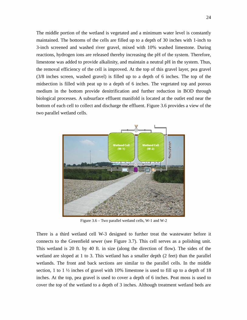
The middle portion of the wetland is vegetated and a minimum water level is constantly maintained. The bottoms of the cells are filled up to a depth of 30 inches with 1-inch to 3-inch screened and washed river gravel, mixed with 10% washed limestone. During reactions, hydrogen ions are released thereby increasing the pH of the system. Therefore, limestone was added to provide alkalinity, and maintain a neutral pH in the system. Thus, the removal efficiency of the cell is improved. At the top of this gravel layer, pea gravel (3/8 inches screen, washed gravel) is filled up to a depth of 6 inches. The top of the midsection is filled with peat up to a depth of 6 inches. The vegetated top and porous medium in the bottom provide denitrification and further reduction in BOD through biological processes. A subsurface effluent manifold is located at the outlet end near the bottom of each cell to collect and discharge the effluent. Figure 3.6 provides a view of the two parallel wetland cells.
Figure 3.6 – Two parallel wetland cells, W-1 and W-2
There is a third wetland cell W-3 designed to further treat the wastewater before it connects to the Greenfield sewer (see Figure 3.7). This cell serves as a polishing unit. This wetland is 20 ft. by 40 ft. in size (along the direction of flow). The sides of the wetland are sloped at 1 to 3. This wetland has a smaller depth (2 feet) than the parallel wetlands. The front and back sections are similar to the parallel cells. In the middle section, 1 to 1 ½ inches of gravel with 10% limestone is used to fill up to a depth of 18 inches. At the top, pea gravel is used to cover a depth of 6 inches. Peat moss is used to cover the top of the wetland to a depth of 3 inches. Although treatment wetland beds are

25
usually slightly sloped to allow a horizontal flow, the Greenfield wetlands have a horizontal bed and work like large storage buckets.
Figure 3.7 – Third wetland cell, W-3
3.2.3 WETLAND MEDIA Three different types of screened, river-washed gravel are used as wetland medium. A larger size of 1.5 to 3 inches gravel is used in the front section of the parallel wetlands in order to reduce the potential of clogging. A smaller size of 1 to 3 inches gravel is used in the middle section of the parallel wetlands. The front section of the polishing wetland is filled with 1 to 3 inches of gravel, but the middle section is filled with 1 to 1 ½ inches of gravel. Pea gravel is on the top of the middle section to support vegetation growth. The pea gravel layer is laid at 6 inches thickness. An additional thin layer (3 to 6 inches) of peat moss is placed on top of the pea gravel to provide thermal insulation over the winter months. All the gravel used is mixed in with 10% crushed limestone (by volume) to ensure adequate alkalinity for nitrification. The bottom of the wetland cells is lined with EPDM liners especially designed for pond liner application. Figure 3.8 shows different type of wetland gravels. 3.2.4 DOSING TANKS The wetland system has one surge tank and four dosing tanks or lift stations at different

26
Figure 3.8 – Wetland media
locations in the system (see Figure 3.3). The surge tank is located at the inflow part of the entire system collecting wastewater from both north and south part of the rest stop. The first dosing tank, LS-1, doses the parallel wetlands, W-1 and W-2. LS-1 receives inflow from the second septic tank, ST-2. The second dosing tank, LS-2, is placed following W-1 and W-2. LS-2 re-circulates part of the treated wastewater from W-1 and W-2 to ST-2. Dosing tank, LS-3, after the third wetland cell, transmits a portion of the wastewater to the biofield. The fourth dosing tank, LS-4, pumps wastewater from the third wetland cell back to the main westbound lift station, from where it is finally sent to the Greenfield wastewater treatment plant. Gravity flow exits from ST-2 to LS-1, from the two wetland cells to LS-2, and from W-3 to LS-3. Each of the lift stations have a cross-sectional area of 8.5 ft by 5.5 ft with a depth of 7 ft. Each lift station is equipped with two pumps. The pumps used in the lift stations are duplex pumps. Except for LS-3 being controlled by the SCADA system, the rest pumps operates on a level float control system. Wastewater inflow to these lift stations is not the same, and the level floats are set at different heights in each lift station to accommodate varying flow rates. For example, in LS-1, the ON/OFF floats within the tank are separated by a vertical elevation of approximately 24 inches that translates to 700 gallons per dose. The number of doses required will vary based on actual daily flow rate, precipitation, and recycle percentage. The pumps in the LS-1 have a capacity of 50 gpm (gallon per minute). An alarm is set approximately 6 inches above the ON float to signal the failure of the pump in the lift station. A lag is set above the alarm to initialize an “All ON” condition to ensure that the alternate pump functions while the other pump is out of service.

27
The wastewater flows from W-1 and W-2 to the distribution box that serves as a flow splitter (FS in Figure 3.3 and see Figure 3.9) from where 83 percent of the influent is directed to the recirculation dosing tank, LS-2. The recirculation percentage can be adjusted by plugging holes in the distribution box. The ON/OFF floats in LS-2 are separated by an approximate height of 30 inches that provides 875 gallons per dose. The pumps have a capacity of 50 gpm.
Figure 3.9 – Flow splitter FS
The rest of the 17 percent of the wastewater from the distribution box flows by gravity to the third wetland cell, W-3. There is a level adjust sump at the end of the wetland that controls flow out of the cell into the biofield lift station, LS-3. The pump within LS-3 needs to dose a small amount of water. Initially it was approximated as 100 gallons to the biofield on a timer-activated cycle at a frequency of four times a day - a total of 400 gallons per day. Between the two floats in the tank, the OFF float prevents the pump from running dry in the event of manual pumping, while the other float works as an alarm to the pump indicating high water in the tank. The floats are separated by approximately 39 inches. The biofield lift station, LS-3, overflows to the fourth lift station, LS-4. Pumps within LS-4 lift the treated water and send it through the force main to the original lift station that pumps water to the wastewater treatment plant. The floats within the LS-4 dosing chamber are separated by 18 inches. LS-4 is expected to dose 64 times a day for a total of 9000 gallons. 3.2.5 BIOFIELD

28
At the tail end of the wetland system, a biofield was constructed to provide treatment to a small amount of wastewater (see Figure 3.10). The biofield is essentially a sand mound with the top seeded with prairie grass. It has a base area of 1652 square feet with a bed area of 333 square feet. The biofield was expected to treat the wastewater by denitrification, and finally dispose the treated effluent by evapotranspiration and infiltration to the subsoil.
Figure 3.10 – Biofield
3.2.6 WETLAND PLANTS Wetland plants provide storage sites for carbon and nutrients and play a role in the movement of gases to and from the wetland substrate. Oxygen is transported from the air through the plant into the root zone. This ensures that aerobic respiration can be maintained in the non-photosynthetic portion of the plant tissues buried in the anoxic substrate. Recent research has shown that wetland plants do not increase oxygen transfer significantly and, thus, contributions in the treatment process are not substantial (Juwarkar et al., 1995, Huang et al., 2000). However, the wetland plants are still considered an important part of the system as they (1) increase the rate of water loss through evapotranspiration, (2) provide a large surface area for bacterial growth through an extensive root system, and (3) provide aesthetic value to the treatment facility. About 3,280 plants of 13 different species were planted in the three wetland cells. To promote diversity and maintain aesthetic value, a variety of perennial bulrushes, sedges,

29
grasses, and a number of flowering species were planted. Examples are shown in Figure 3.11. More details are available at the website (https://engineering.purdue.edu/Research Groups/Wetland) Wetland plants are discussed in more detail in Chapter 5 of this report.
Figure 3.11 – Examples of wetland plants (Left panel: Scirpus Cyperinus
[wool grass] ; Right panel: Helenium Autumnale[Sneezeweed]) 3.3 WETLAND OPERATION SCHEME Some preliminary tests conducted prior to construction of the wetlands indicated that wastewater from the rest area had the following characteristics:
- BOD5: 450 mg/L - NH3-N: 150 mg/L - TSS: 180 mg/L
The hydrology of a conventional SFCW was judged as being inadequate to provide significant primary and secondary treatment to such high strength wastewater. Conventional SFCWs are constructed as a horizontal plug-flow reactor. The treatment in the wetland is accomplished by the microorganisms that come in contact with the wastewater. In the saturated substrate of the wetland, the microorganisms break down the pollutants. Treatment efficiency depends mainly on reduction in BOD5, NH3-N, and TSS.

30
Microorganisms consume oxygen to break down organic carbon to carbon dioxide (CO2), and BOD5 is reduced. Microorganisms also reduce the NH3-N level by a two-step process - nitrification and denitrification. Nitrogen is usually present in the form of nitrate, nitrite, and ammonia or ammonium ion, with the predominant form being nitrate. In the first step of the two-step processes, nitrification-ammonia and ammonium ions are transformed into nitrate. In the second step, denitrification-nitrate is converted to nitrogen (N2) gas. So denitrificaion completes the nitrogen reduction/removal process. Nitrifying bacteria break up the pollutant in the presence of oxygen during nitrification. On the other hand, denitrification processes require an anoxic environment. Conventional wetlands have dissolved oxygen (DO) typically below 1.0 mg/L (US EPA, 2000; Behrends et al., 2001). This limited amount of oxygen can lead to a complete halt of nitrification. So nitrogen removal efficiency can be improved greatly by increasing the amount of oxygen present in the wetland substrate. Research (Wieder et al., 1989) shows that there are three features that can be incorporated in a conventional SFCW to improve treatment performance. These are (1) the wetland may be divided into segments (as plug flow systems) that can operate and drain separately, (2) arrangements to allow step feeding the influent into the wetland, and (3) arrangements to allow for effluent recycling (Wieder et al., 1989). Scientists at the Tennessee Valley Authority (TVA) have developed a unique and patented SFCW system that is filled and drained alternatively at a frequency of two hours per cycle (Behrends et al., 2001). This technology (illustrated in Figure 3.12) has shown high ammonia removal for a variety of wastewater streams (Behrends et al., 2001). This fill and drain concept (US EPA, 2000) has been applied to a three-cell SFCW system in the village of Minoa, NY, and has shown some success in producing effluent quality that is better than the conventional plug flow SFCW systems (e.g. three cells in series). The Minoa system also has two cells in parallel and is operating at an alternating fill and draw mode followed by a third cell designed as a conventional plug flow reactor, similar to the design adopted at the Greenfield site. The fill and drain scheme has shown some success as it can increase the amount of oxygen in the wetland substrate - a key component for removal efficiency. During the drain cycle, oxygen from the air diffuses through the thin film of water surrounding the plant roots and the biofilm on the wetland substrates. During the fill cycle, plant roots and biofilms on the substrate are filled by the anoxic wastewater (Figure 3.12), and the microorganisms get enough oxygen to break down the pollutants. Because of the large

31
O2
Drain cycle Fill cycle Figure 3.12 – Illustration of oxygen diffusion during fill and drain cycle
surface area present in the SFCW due to plant roots and substrates, the oxygenation of the rhizosphere and the substrate biofilms is substantial and rapid. This can potentially decrease the long HRT required for the nitrogen removal associated with the conventional SFCW systems. Two parallel wetlands operating under the fill and drain scheme and one conventional polishing wetland cell are being used in the Greenfield rest area. It was expected that the modified design would reduce the effluent concentration to meet permit limits. 3.4 INSTRUMENTATION AT THE GREENFIELD SITE Some of the objectives behind the construction of the Greenfield’s wetland treatment system were to provide an understanding of the function of the constructed wetlands, quantify pollutant removal, and develop management strategies. So the treatment facility has been instrumented to collect data at various locations in the system. These collected data are being used to model the system and to assess its performance. The following sections provide a description of the instruments installed within the wetland system. 3.4.1 FLOW MEASUREMENT

32
The system has both open channel flow as well as pressurized flow. For open channel flow measurements, two types of flow meters are in place - three ultrasonic flow meters (see Figures 3.13 and 3.14) and a V-notch weir (Figure 3.15) are used at specific locations in the wetland system.
Figure 3.13 – Ultrasonic flow meter
(Source: http://www.environmental-expert.com/technology/greyline/level.htm)
Figure 3.14 – Flow meter detecting the amount of flow in the open channel
(Source: http://www.greyline.com/pdf/SLT32.pdf)
A 22.5o V-notch weir (F-1 in Figure 3.3) is used along with an ultrasonic flow meter between the septic tanks (Figure 3.15). Both are used together to record the effluent flow rate from the first septic tank. This facility uses a Greyline OCF-IV flow meter. This non-contacting ultrasonic sensor is mounted above the liquid level. It has a user friendly calibration system and it is easy to set up the monitor to display measurements in specified units (ft, cm, gallons, liters, etc). Standard sensors can measure a depth of up to 32 ft. A picture of the V-notch weir is shown in Figure 3.15 for illustration purposes.

33
Figure 3.15 – Flow over the V notch weir is being measured by the flow meter F-1
Two other flow meters (F-2 and F-3 in Figure 3.3) are Palmer-Bowlus flumes equipped with ultrasonic level sensors. They are simple and effective flow measuring devices. Four inch size flumes are used on the site and are recommended for a flow range of 5-55 gpm. One flume, F-2, is located downstream from the parallel wetlands to measure the flow going to the third polishing wetland. The second flume F-3 is placed after the polishing wetland cell W-3. EMCO Unimag 4411e magnetic flow meter (Figure 3.16) is sued after the surge tank to measure the total inflow to the wetland system. Sparling FM657 magnetic flow meters (Figure 3.17) are being used after the dosing chambers to measure the flows. A magnetic flow meter is a volumetric flow meter that does not have any moving parts, and is ideal for wastewater application or any dirty liquid that is conductive or water-based.
Figure 3.16 – EMCO Unimag 4411e magnetic flow meter (Source: http://www.advancedflow.com/pdf/Data_Sheets/4411e_DS.pdf)

34
Figure 3.17 – Sparling FM657 magnetic flow meter
(Source: http://www.muellersales.com/pdf/spa_tigermag_fm657.pdf)
Figure 3.18 – Magmeter working principle
(source: http://www.ferret.com.au/Specsonline/files/212.pdf) Magnetic flow meters operate based on Faraday’s law of induction (Figure 3.18). In electromagnetic measurement, the flowing medium corresponds to a moving conductor whose induced velocity is proportional to the flow velocity, and is detected by two measuring electrodes and then transmitted to an amplifier. Flow volume is computed on the basis of the pipe’s diameter. The constant magnetic field is generated by a switched direct current of alternating polarity. The mag flow meters typically measure flow with velocity ranging from 0.01 to 10 m/s. 3.4.2 WATER QUALITY SAMPLING To understand how well each component of the wetland system is working, four automatic samplers (see Figure 3.19) were installed to collect wastewater samples at various points in the system. These samplers are the 6712R refrigerated samplers by

35
Teledyne Isco. The first sampler, AS-1 was installed before the septic tank, ST-2, to sample effluent from ST-1. The sampler AS-2 was placed after the second septic tank, while AS-3 is placed after the parallel wetlands on the recirculation branch. The fourth and the last sampler, AS-4 collects effluents from the third wetland cell. Their locations are schematically shown in Figure 3.3.
Figure 3.19 – Water Quality Sampler
(Source: http://www.isco.com/products/products3.asp?PL=201202010) The 6712FR refrigerated samplers are designed to withstand harsh indoor and outdoor environments. The cabinet of the refrigerator is corrosion proof, and molded from polyester resin fiberglass and supported by a stainless steel frame. A UV-resistant gel coating provides a smooth, non-porous finish for added protection and easy cleaning. The inside of the refrigerator is thick-foamed to provide insulation to preserve samples at EPA recommended 39oF (4oC). It also has built-in heater to automatically ensure that the samples will not freeze. The sampler components are
(a) Controller (b) Center section (c) Peristaltic pump (d) Liquid detector (e) Strainer (f) Suction line
36
(g) Stainless coupling (h) Pump tube (i) Bulkhead fitting (j) Discharge tube (k) Distributor arm and spring.
The controller in the sampler allows selecting between standard programming and extended programming mode. In standard programming mode, the controller allows a step by step sampling sequence. Extended programming mode can be used to choose more complex options including “smart sampling” notification triggered by any of up to 16 inputs. The strainer in the sampler prevents clogging of the suction side. Isco provides four different types of strainer to match application requirements. When the sampler takes a sample, it draws liquid through the strainer that is connected to the pump tube by a suction line. The sample passes the liquid detector, which senses the liquid. From the detector, the sample follows the pump tube through the pump to the bulkhead fitting and through the discharge tube to the sample bottle. All four samplers used in the wetland system have a 24 bottle sampling kit. A typical sampling cycle consists of
(1) The sampler moves the distributor arm over the bottle that is to receive the sample. The bottle number can be specified from the controller.
(2) The pump reverses for pre-sample purge. (3) The pump direction changes, filling the suction line. (4) When the detector senses liquid, the sampler begins measuring the sample. (5) After depositing the sample, the pump again reverses for a post-sample purge.
Samples from the four locations have been collected on an intermittent basis since the wetland system has been in operation. 3.4.3 WEATHER STATION A weather station was installed at the site to collect data on rainfall, wind speed, temperature, and evapotranspiration. These data are important to determine hydrologic balance within the wetland system. These data could also help to correlate reaction rates
37
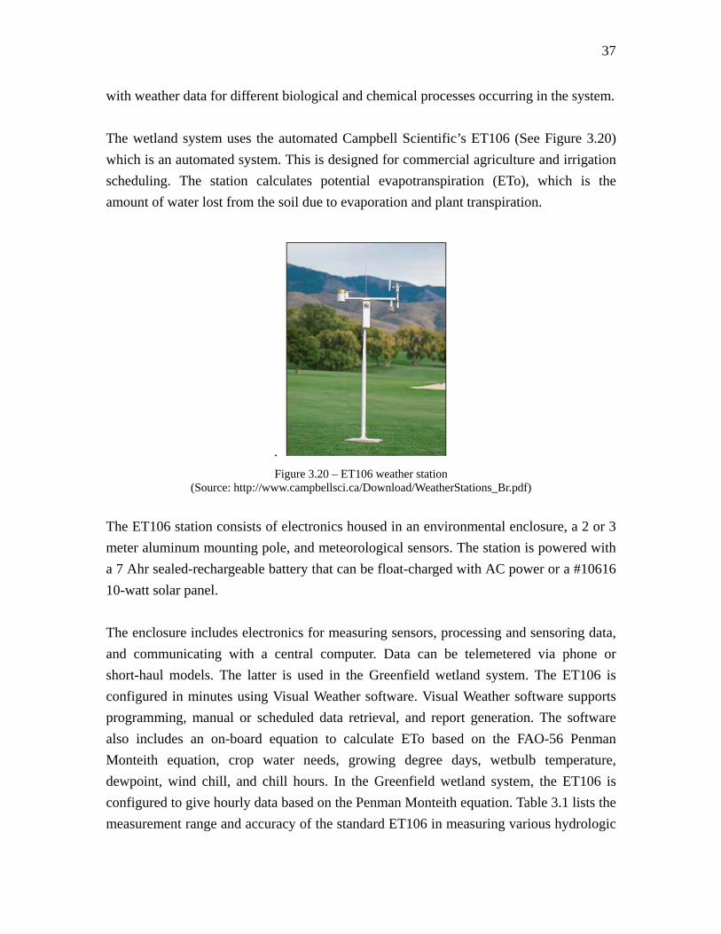
with weather data for different biological and chemical processes occurring in the system. The wetland system uses the automated Campbell Scientific’s ET106 (See Figure 3.20) which is an automated system. This is designed for commercial agriculture and irrigation scheduling. The station calculates potential evapotranspiration (ETo), which is the amount of water lost from the soil due to evaporation and plant transpiration.
. Figure 3.20 – ET106 weather station
(Source: http://www.campbellsci.ca/Download/WeatherStations_Br.pdf) The ET106 station consists of electronics housed in an environmental enclosure, a 2 or 3 meter aluminum mounting pole, and meteorological sensors. The station is powered with a 7 Ahr sealed-rechargeable battery that can be float-charged with AC power or a #10616 10-watt solar panel. The enclosure includes electronics for measuring sensors, processing and sensoring data, and communicating with a central computer. Data can be telemetered via phone or short-haul models. The latter is used in the Greenfield wetland system. The ET106 is configured in minutes using Visual Weather software. Visual Weather software supports programming, manual or scheduled data retrieval, and report generation. The software also includes an on-board equation to calculate ETo based on the FAO-56 Penman Monteith equation, crop water needs, growing degree days, wetbulb temperature, dewpoint, wind chill, and chill hours. In the Greenfield wetland system, the ET106 is configured to give hourly data based on the Penman Monteith equation. Table 3.1 lists the measurement range and accuracy of the standard ET106 in measuring various hydrologic

38
components. Table 3.1 – Operating range and measurement accuracy of the weather station ET106.
Hydrologic Component Operating Range Measurement Accuracy Solar Radiation-Silicon photocell sensor Absolute error in natural daylight is 5%
maximum, ±
± 3% typical. Rainfall-Tipping bucket rain gauge ± 1% accuracy at 2 inches per hour or less
rainfall.
Wind Speed-Cup anemometer 0 to 49.5 m/s (0 to 110 mph)
± 0.11 m/s (± 0.25 mph) when <10.1 m/s (22.7 mph); ± 1.1 of true when >10.1 m/s (22.7 mph).
Wind Direction- Weather vane 360o mechanical, 356o electrical. Accuracy ± 4o.
Relative humidity 0 to 98% RH. ± 3% for 0-90% RH, ± 5% for 90-98% RH. Air temperature -25 to 60oC ± 0.8oC accuracy.
(Source: http://www.campbellsci.ca/Download/WeatherStations_Br.pdf)
3.5 DESCRIPTION OF THE DATA Construction of the system started in the winter of 2002. Installations of all the instruments except the weather station were completed by February of 2004. The weather station was installed two months later in mid April. The data collection from the flow meters started in September 2003, a few months before the complete installation of instruments. From Dec 2003, drinking water data has been recorded. On Feb 10th, 2004, data from the INDOT datalogger were collected for the first time. On the same day, wastewater samples from different locations of the wetland system were also collected. But, later that month, LS-3 and M-2 had operation problems and it was found that INDOT datalogger was not grounded. The problems were quickly resolved. However, during the last two years of operation of the system, all the instruments except the weather station were out of service from time to time. They were repaired and soon put back to the system. Table 3.2 provides a time line describing when some of the measurement devices were not functional during wetland operations. Availability of data from various instruments is summarized in Table 3.3. The summary is prepared on 10-day intervals. The “P” in the table indicates the data are partly available during those entire 10 days. Complete availability of the data in the table is indicated by “O”. A preliminary analysis of the data shows that some of the recorded values are not reasonable and are designated by “?”. The table also shows that the flowmeters have recorded daily flow values rather than hourly flow values during the first few months of operation. From Feb

39
Table 3.2 - Wetlands Equipment Chronology Date Event
Feb. 3, 2004 Finished connecting magmeters M1 thru M4 to INDOT datalogger. Reset magmeter totalizers
Feb. 10, 2004 Site visit, collected data from INDOT datalogger and grab samples. Changed record interval to 1 Hr. on Greylines.
Feb. 23, 2004 LS3 shut down. INDOT datalogger found to be not grounded. M2 showed bad coils. Collected data from INDOT datalogger and Greylines. Reprogrammed magmeters and INDOT datalogger M1 Full Scale Output = 140GPM. Reset totalizer @ 2:46PM - was 3916 counts M2 Full Scale Output = 100GPM M3 Full Scale Output = 75 GPM M4 Full Scale Output = 200 GPM. Reset totalizer @ 2:51PM - was 3716 count
March 5, 2004 Grounded Telog datalogger. Collected trend and event data. April 15, 2004 Installed weather station. Wind direction not accurate (+/- 10o). Collected flow data. Magmeter
flow data diskette corrupted. May 19, 2004 Site visit, collected data from INDOT datalogger, weather station & open channel flowmeters.
Connected communication wires from weather station into water softener building. Noted that wetlands had been bypassed since March LS3 alarm was active and cell #3 was flooded.
June 7, 2004 Site visit, collected data from INDOT datalogger & open channel flowmeters. Installed CR10 on magmeters.
June 15, 2004 Site visit, collected data from CR10 on magmeters. July 23, 2004 Site visit, collected data from CR10 on magmeters and F1, F2, F3, and weather station. Pulled
monitor on F3 for repair. Sept. 22, 2004 Site visit, reinstalled F3. Oct. 21, 2004 Site visit, reinstalled M2. Nov. 23, 2004 Site visit, collected data from CR10 on magmeters and F1,& F3, and weather station. Pulled
monitor on F2 for repair. Pulled remote transmitter on M2 for repair. Dec., 2005 Started the setup for SCADA system. Flow data collection was temporally unavailable. July, 2006 Flow conditions and some other measurements were ready to be downloaded on the website.
Table 3.3 – Wetland Data Condition 2003
1 11 21 1 11 21 1 11 21 1 11 21 1 11 21 1 11 21 1 11 21 1 11 21 1 11 21 1 11 21 1 11 21 1 11 21M1M2M3M4F1 P D D D D D D D D DF2 P D D D D D D D D DF3 P D D D D D D D D D
Drinking O O OWeather P P
20041 11 21 1 11 21 1 11 21 1 11 21 1 11 21 1 11 21 1 11 21 1 11 21 1 11 21 1 11 21 1 11 21 1 11 21
M1 P 3 3 P 3 P ? ? ? P 5 5 P P P P O O O O O O O O O O O O O O O OM2 P 3 3 P ? ? ? ? ? P 5 5 P ? ? P O O PM3 P 3 3 P 3 P ? ? ? P 5 5 P P P P O O O O O O O O O O O O O O O OM4 P 3 3 P 3 P ? ? ? P 5 5 P P P P O O O O O O O O O O O O O O O OF1 D D D P O O O O O O O O O O O O O O O O O O O O O O O O O O O O O O O OF2 D D D P O O O O O ? ? ? O O O O O O O O P P O O O O O PF3 D D D P O O O O O O O O O O O O O O O O P P O O O O O P P O
Drinking P P O O O O O O O O O O O O O O O O O O O O O O O O O O O O O OWeather O O P P O O O O O O O O O O O O O O O O O O O O O O O O O
20051 11 21 1 11 21 1 11 21 1 11 21 1 11 21 1 11 21 1 11 21 1 11 21 1 11 21 1 11 21 1 11 21 1 11 21
M1 O P P O O P P O O O O P P PM2 P P O OM3 O P P O O P P O O O O P P P P O O PM4 O P P O O P P O O O O P P P P O O PF1 O O O O O O O O O O O O O P P O O O O O O O PF2F3 O P P O O O P
Drinking O O O O O O O PWeather O O O O O O O O O O O O O O O P P O O O O O O O P
M1, M2, M3, M4: Minimum Unit in Minute O: Full Data Available P: Partial Data Available ?: Questionable D
P
aF1, F2, F3, Drink., Weather: Minimum Unit in Hour 3: 3-Min Interval 5: 5-Min Interval D: Daily Interval
Sep Oct Nov DecMay June July AugJan Feb March April
Jan Feb March April May June July Aug Sep Oct Nov Dec
Jan Feb March April May June July Aug Sep Oct Nov Dec

40
2004, the flowmeters started collecting data on hourly basis. Similarly, magmeters though programmed to record flow data every minute, have recorded the data every 3 to 5 minutes during the first year of operation. Unfortunately, most of the time, magnetic flow meter M-2 was out of service. Flow meter F-2 has not recorded any data during the entire year of 2005. So, although a large data set is available from the system’s operation, there are only few instances when all the instruments provided uninterrupted data. In the following paragraphs, the data are further described. 3.5.1 FLOW METER DATA Flow meter data from F-1 corresponds to wastewater inflow rate in to the wetland system. Available F-1 data were compared with drinking water data each month to confirm the accuracy of flow meter readings because wastewater is generated from the drinking water or tap water. These two data sets should show similar trends and should be strongly correlated to each other. The drinking water data includes usage from both the north and south rest areas. Care needs to be exercised as wastewater from both sides was not always directed to the wetland system. The last drinking water and F-1 data set were recorded over a year ago (Table 3.3). Figure 3.22 shows drinking water and F-1 data recorded in June, September, and October-November of 2004. In September 2004 (Figure 3.22b), the flow meter data exceeded the drinking water values by a large difference indicating that the data recorded by F-1 was inaccurate. But, during October-November, the F-1 data matched very well with the drinking water data (Figure 3.22c). On other hand, the F-1 data in June of 2004 shows values that are about half the value of the drinking water data set (Figure 3.22a). During this time, the wetlands were receiving wastewater only from the north rest area. However, the wetlands had not received any wastewater for few days during this month (see flow rates of F-1 between day 12 to day 16 in Figure 3.22a). Data from the flow meters F-1, F-2, and F-3 were also compared to drinking water data, and some of these results are shown in Figure 3.23. Specifically, data from June and October 2004 are studied here. Since the inception of the flow meters, F-1 and F-2 data along with drinking water have been available without interruption during these periods. However, data from these flow meters are not always accurate. For instance, data

41
0
2000
4000
6000
8000
10000
12000
14000
0 5 10 15 20 25 30
Time (Days)
Flow
(gpd
)F1 dataDrinking Water
0
10000
20000
30000
40000
50000
60000
70000
80000
90000
100000
0 5 10 15 20 25 30
Time (Days)
Flow
(gpd
)
drinking waterF1 data
Figure 3.22(a) – Drinking water and Figure 3.22(b) – Drinking water and F-1 recorded data in June, 2004 F-1 recorded data in September, 2004
0
1000
2000
3000
4000
5000
6000
7000
8000
0 5 10 15 20 25 30 35
Time (days)
Flow
(gpd
)
F1 dataDrinking water
Figure 3.22(c) – Drinking water and F-1 recorded data from Oct 22 to Nov 22, 2004
recorded by F-2 exceed both F-1 data and drinking water data as shown in Figure 3.23a. Indeed, on some days the discrepancy between F-2 data and drinking water data is more than 700 gallons per hour. The data do show some similar trends in that the peaks and troughs are fairly consistent in time. Similarly, F-2 data are very high in Oct. 2004 as seen in Figure 3.23c, even though the timing of the peaks and troughs are again replicated. Data from F-3 were not always consistent either. Figure 3.23b is an example of F-3 data that does not track to drinking water data. For about eight days in October, 2004, F-3 data were reasonable but again rose to very high values (Figure 3.23d). Flow meters, F-2 and F-3 are expected to have fairly large errors, especially for low flows, but these data indicate that F-2 and F-3 data need to be viewed carefully. F-1 data tend to be more reliable when compared to drinking water data because F-1 is a V-notch weir, while F-2 and F-3 are Palmer Bowlus flumes. 3.5.2 MAGNETIC FLOW METER DATA

42
0
200
400
600
800
1000
1200
1400
0 5 10 15 20 25 30
Time (Days)
Flow
(gph
)
F2 data
dw data
F1 data
0
5000
10000
15000
20000
25000
30000
35000
0 5 10 15 20 25 30
Time (Days)
Flow
(gph
)
F3 Data
Dw data
Figure 3.23(a) – Drinking water and recorded Figure 3.23(b) – Drinking water and F-3 data from F-1 and F-2 in June, 2004 recorded data in June, 2004
0
100
200
300
400
500
600
700
800
0 2 4 6 8 10
Time (Days)
Flow
(gph
)
F2 data
Dw data
F1 data
0
5000
10000
15000
20000
25000
30000
0 2 4 6 8 10
Time (Days)
Flow
(gph
)
F3 data
Dw data
Figure 3.23(c) – Drinking water, F-1, and F-2 Figure 3.23(d) – Drinking water and F-3 recorded data in last 11 days in Oct., 2004 recorded data in last 11 days in Oct, 2004
Magmeters record the flow rates from the dosing tanks where the water flows under pressure. Since the operation of the wetland system, all the magmeters were simultaneously functional only during a short period from October 22nd to November 22nd, 2004. Magmeters M-1, M-2, and M-3 recorded data most of the time during 2004, while in 2005 these were in operation only for few months (see Table 3.2). Figure 3.24 shows some samples of magmeter readings, and needs to be interpreted in conjunction with Figure 3.3. The magmeters are located immediately downstream of lift stations and reflect the magnitudes of flowrates and intermittency of the pumps. For instance, Figure 3.24a shows data from M-1 for some days in April 2004. M-1 flow is dictated by pumping schedule of LS-1. The figure indicates the LS-1 pumps are operating a little over 50 gpm. Similarly, M-3 data in Figure 3.24b indicate that LS-3 pumps are operating at about 18 gpm in April of 2004. This data also indicates that the pumps in LS-3 switch on less frequently than LS-1. Figure 3.23c shows a sample of M-4 data that indicates LS-4 is operating at 22 gpm on an average. The data recorded by the magmeters is not always consistent. For instance, M-2 data in Figure 3.24d for a different time period

43
indicates an average pumping rate of 60 gpm for LS-2. This is in contrast to the 5 gpm pumping rate shown in Figure 3.24e. Given the high recycling rate, the data in Figure 3.24d for M-2 would seem to be reasonable, as even a continuous pumping rate of 5 gpm in Figure 3.24e from LS-2 cannot accommodate the recycle volume.
0
10
20
30
40
50
60
70
0 2 4 6 8 10
Time(Days)
Flow
(gpm
)
M1data
0
5
10
15
20
25
0 2 4 6 8 10
Time(Days)
Flow
(gpm
)
M3 data
Figure 3.24(a) – M-1 recorded data in April Figure 3.24(b): M-3 recorded data in April 21 to 30, 2004 21 to 30, 2004
0
5
10
15
20
25
30
35
40
45
50
0 2 4 6 8 10
Time(Days)
Flow
(gpm
)
M4 data
0
10
20
30
40
50
60
70
0 5 10 15 20 25
Time (Days)
Flow
(gpm
)
M2 data
Figure 3.24(c) – M-4 recorded data in April Figure 3.24(d) – M-2 recorded data in Nov 11 21 to 30, 2 004 to Dec 16, 2005
0
1
2
3
4
5
6
7
0 2 4 6 8 10
Time(Days)
Flow
(gpm
)
M2 data
Figure 3.24(e) – M-2 recorded data in last 10 days in Oct., 2 004

44
3.5.3 WEATHER STATION DATA Data had been recorded continuously by the weather station since its installation until the first week of June, 2005. Sample of rainfall data in October, 2004, are shown in Figure 3.25. Rainfall data is the primary component of the hydrologic budget that is produced by the weather station.
0
5
10
15
20
25
30
1 2 3 4 5 6 7 8 9 10 11 12 13 14 15 16 17 18 19 20 21 22 23 24 25 26 27 28 29 30 31
Time (Days)
Rai
nfal
l (m
m)
Rainfall
Figure 3.25 – Rainfall data recorded data in October, 2004
It would appear that the data have errors and inconsistencies that make interpretation more challenging.

45
CHAPTER 4
HYDROLOGIC PERFORMANCE
4.1 INTRODUCTION As described in the previous chapter, the entire system includes a pair of wetlands with alternate fill and draw scheme along with recirculation. This makes the system rather complex for the estimation of hydraulic retention time (HRT) - which is commonly used as a wetland performance index. HRT estimation is made more difficult because of transient nature of the system with the water level and flowrates fluctuating over time. The model estimates the volume of water in the wetland cells by simulating the performance of the entire system, and computes how depths vary in the wetland cells during fill and drain cycles. The hydraulic model of the Greenfield wetland system was built using a systems approach with the aid of Simulink in MATLAB. With the Simulink model editor, a block diagram representing the entire wetland system was created first. Model simulations were conducted for about 10 consecutive days starting from November 1st to November 10th, 2004. The model was then validated using a ten-day consecutive data set from October 2004. The model computations were based on one second time step. Subsequent sections in the chapter describe how each of the elements of the wetland complex was represented in the model. Topics covered in this chapter are validation using observations, and recognizing the limitations of the model. Details of the modeling effort are available in Sultana (2006). 4.2 MODEL DESCRIPTION Each part of the wetland system was modeled to mimic its operation as closely as possible. Description of each component follows: Septic Tanks: The two septic tanks are capsule-shaped containers. The maximum

46
diameter of the tank is 8 feet, and the inlet and outlet pipes are 6 inches in diameter that are placed at a height of 7 feet from the bottom of the tank. Consequently, the tanks are always full to a height of 7 feet, and the wastewater effluent coming through the inlet pipe passes out of the tank by the outlet pipe after a small time lag. As in Figure 3.22c, F-1 data was compared with drinking water data, and it was observed that the time series are nearly identical indicating a small time lag that is practically negligible. In the model, septic tanks are designed like a gate through which the wastewater flows out almost instantaneously towards the parallel wetlands. Lift Stations: The system has 4 lift stations (LS-1, LS-2, LS-3 and LS-4). The model includes all the four lift stations. LS-1, LS-2, LS-3 have a cross section of 8.5 feet by 5.5 feet with a full depth of 9 feet each. LS-4 has a circular cross section with diameter of 4 feet and a full depth of 9.5 feet. All the lift stations have two pumps each. During the completion of the wetland system, it was planned to run the pumps alternatively during slack hours in all the lift stations. But, because of increased usage of the rest area, both the pumps in LS-1 and LS-2 operated together to meet with the increased demand (see Figure 3.24a and d). On the other hand, the observed data shows that the demands on LS-3 and LS-4 were relatively small, and so the two pumps in those two stations operate alternatively (see Figues 3.24b and c). All the pumps stop pumping as the water depth falls to a height of 15 inches from bottom. In the model, LS-1 and LS-2 were modeled with two pumps operating together when the water depth rises to 39, and 45 inches respectively. The model was built to run with a single pump for LS-3 and LS-4 that operate when the water level rises to 50, 55 inches, respectively. Change of water level within the lift station was modeled by
LWtQ
dtdh
×=
)( ( 4 .1 )
where, is the width, and is the length of the base area of the lift station, is
the flow rate in the lift stations at time , and
W L )(tQ
tdtdh is the change of water level within
the lift station. Actuators: There are two actuator switches (ACT-1 and ACT-2) in the system. ACT-1 precedes the parallel wetlands and generates a signal to fill either of the parallel wetland cells, while ACT-2 is downstream of the two parallel wetland cells and controls emptying

47
of the cells. This ‘draw and fill’ scheme operates on a time-based switch such that while W-1 is filling, W-2 is draining and vice versa. The switch occurs once a day from Tuesday to Friday, but twice a day from Saturday to Monday to accommodate the higher flow rates expected during weekends. In the model, both the actuators were modeled as a single element that sends a signal to alternate cells once daily from Tuesday to Friday and twice daily from Saturday to Monday to drain and fill alternatively. Wetland cells: The two parallel wetlands and the third polishing wetland work like large buckets. The parallel cells have a depth of 3 feet but are designed to have maximum water level of 2.75 feet to ensure subsurface flow. When the water level rises above the depth of 2.75 feet, wastewater overflows immediately through a pipe of 4 inches diameter regardless of the drain signal. On the other hand, when the wetland receives the drain signal from ACT-2 during the draining cycle, a valve opens up and the effluent is drained through another 4 inch diameter pipe. The wetlands are drained until the water level in the cells drop to 1.25 feet. Thus, a draining and an overflow mechanism have to be incorporated. This minimum depth of water in the cells is maintained to ensure plants survival between drain and fill cycles. However, the polishing wetland cell operates differently when compared to the parallel wetland cells. This wetland has a depth of 2 feet and is designed to have a constant water depth of 1.5 feet. Whenever the water depth rises above this threshold, water is instantaneously drained out from the wetland through a 6 inch diameter pipe. The wetlands not only receive wastewater but also rainfall that is added to the wetland cells directly regardless of whether the cells are filling or draining. In the model, each wetland cell is designed as a container of trapezoidal cross section. The parallel wetlands are filled during their filling cycle and drained during the drainage cycle. The water level change in the wetland cell is determined by the following equation
η))(6))((6()(
thLthWtQ
dtdh
++= (4 .2)
where, is the difference in inflow ( ) to and outflow ( ) from the wetland, )(tQ inQ outQ
dtdh is the change of depth within the wetland, is the width of base, is the length
of the base of the wetland cell, and is the depth of water at time in the cell. The porosity,
W L
)(th tη , in equation (4.2) is used to reduce the volume of the wetland to effective
volume. For the parallel wetlands, is effluent flow rate from LS-1 along with rainfall rate, and is the overflow and draining rate through overflow and drain pipes
inQ
outQ

48
connected with the wetlands. Similarly, in the polishing wetland is the rainfall rate added with the small percentage of flow directed from the parallel wetlands. When the water level in the parallel wetland rises above 2.75 feet, then the excess water is drained out through a overflow pipe. Similarly, the excess water rising above 1.5 feet is drained out from the polishing wetland. The parallel wetlands are also drained through a drain pipe in response to a time-based switch. The quantity for overflow was modeled as:
inQ
outQ
)(2 max11 hhgACQ doutdoutout −= , for (4 .3) maxhh >
whereas, for draining was modeled as: outQ
)(2 min22 hhgACQ doutdoutout −= , for maxmin hhh ≤≤ (4 .4)
where, , are discharge coefficients, and are outlet pipe areas of the overflow pipes and draining pipes, respectively, and
1doutC 2doutC 1doutA 2doutAg is gravitational
acceleration. The discharge coefficients are introduced to account for the effects of all energy losses including friction losses in the pipes and within the wetland cells along with all other minor losses. in equation (4.3) was taken equal to 2.75 feet for parallel wetlands and 1.5 feet for polishing wetland. in equation (4.4) was taken equal to 1.25 feet.
maxh
minh
The third wetland cell is modeled as a horizontal flow reactor. The water level in the cell is maintained at a constant height of 1.5 feet. Response to overflow is instantaneous and effluent flows out through a 6-inch diameter pipe. 4.3 MODEL CALIBRATION The model was calibrated using the consecutive 10-day data starting from 1st to 10th November, 2004, recorded by different instruments within the wetland system. The inflows to the entire system are F-1 data at the V-notch weir and rainfall data from the weather station (Figure 4.1). Evapotranspiration data were not included at this stage as outflow from the entire wetland complex as it was found small compared to rainfall

49
intensities (See Figure 4.2). Note that the scales of y axis of the two graphs (Figure 4.2a and 4.2b) are different.
0
5
10
15
20
25
30
0 1 2 3 4 5 6 7 8 9 10
Time (Days)
Flow
Rat
e (g
pm),
Rai
nfal
l (gp
m)
F-1 dataRainfall
Figure 4.1 – F-1 data and Rainfall during November 1 to 10, 2004
0
2
4
6
8
10
12
0 1 2 3 4 5 6 7 8 9
Time (Days)
Rai
nfal
l (m
m/h
r)
Rainfall
0
0.05
0.1
0.15
0.2
0.25
0.3
0.35
0 1 2 3 4 5 6 7 8 9
Time (Days)
Evap
otra
nspi
ratio
n (m
m/h
r)Evapotranspiration
Figure 4.2(a) – Rainfall during the first 10 days Figure 4.2(b) – Evapotranspiration during of November, 2004 the first 10 days of November, 2004
The lift stations LS-1, LS-2 were modeled to have flow rates of 50 gallon per minute. These are shown in Figure 4.3a and b. LS-3 and LS-4 were modeled to have a flow rate of 15, 25 gallon per minute respectively (See Figure 4.3c and d). Although the observations from M-2 show that the pump is pumping constantly at an average rate of 5.25 gallon per minute, this value was not used in the simulation because it was determined that the M-2 flow data were erroneous (see discussion in section 3.5). After the wastewater flows out of the parallel wetlands, we note that 83 percent of the outflow is recycled back to the parallel wetlands while the remainder of the 17 percent was directed towards the third wetland cell, which was then compared with the F-2 data (Figure 4.4a). Since, the F-2 data also had problems with magnitude of flow, the model parameters were calibrated by matching the time to peak with the F-2 data set. The discharge coefficients and for the overflow and drain pipes in the parallel 1doutC 2doutC

50
0
10
20
30
40
50
60
70
0 1 2 3 4 5 6 7 8 9 100
10
20
30
40
50
60
0 1 2 3 4 5 6 7 8 9 1
Time (Days)
Flow
Rat
e(gp
m)
simulation result
0
M-2 dataSimulation result
M-1 data
Time (Days)
Flow
rate
(gpm
)
Figure 4.3(a) – M-1 data compared with Figure 4.3(b) – M-2 data compared simulation results with simulation results
0
5
10
15
20
25
0 1 2 3 4 5 6 7 8 9 10
Time (Days)
Flow
rate
(gpm
)
M-3Sim result
0
10
20
30
40
50
60
0 1 2 3 4 5 6 7 8 9 10
Time (Days)
Flow
rate
(gpm
) sim resultM-4
Figure 4.3(c) – M-3 data compared with Figure 4.3(d) – M-4 data compared simulation results with simulation results
wetland cells were selected as 0.6 and 0.04, respectively by calibration using F-2 data as seen in Figure 4.4a. The justification for this small value of of drain pipe is because of the flow through the porous media as well as the drain valve in the drain pipe that opens up during the drain cycle. The observed peaks (in Figure 4.4a) are due to the overflow rates and the troughs are due to the draining of the parallel wetland cells.
2doutC
Similarly, the outflow from the third wetland cell was compared with the F-3 data (Figure 4.4b) and for the overflow pipe in W-3 was chosen as 0.04. For LS-3, the time of pumping also depends on the fraction of the effluent from W-3 flowing to the biofield which was not known. So, in simulations, 17 percent of the effluent was directed towards the biofield while the rest flowed to the Greenfield’s municipal treatment plant.
doutC

51
0
2
4
6
8
10
12
14
16
0 1 2 3 4 5 6 7 8 9 100
2
4
6
8
10
12
14
16
18
20
0 1 2 3 4 5 6 7 8 9
Time (Days)
Flow
rate
(gpm
)
F-2 data
10
F-3 dataCdout=0.04Cdout=0.02
Cdout1=0.6 and Cdout2=0.04
Time (Days)
Flow
Rat
e (g
ph)
Figure 4.4(a) – F-2 data compared with Figure 4.4(b) – F-3 data compared with simulation results ( , 6.01 =doutC 04.02 =doutC ) simulation results ( ,and 0.04). A 02.0=doutC
value of 0.04 was chosen for from wetland cell W-3.
doutC
Sensitivity Analysis Given some of the discrepancy with F-2 data, a sensitivity analysis was conducted to calibrate the model parameters. In the sensitivity analysis, values of each of the parameters ( , , ) were varied by lowering or raising their magnitudes (ranging between 0.2 to 0.8). The sensitivity of the model was qualitatively compared by graphing model output from each run with F-2 data set. It was observed that the model output is sensitive to the initial water level of the lift stations (Figure 4.5c), and timing of drain signal (Figure 4.5a, b). During operation, the parallel wetlands were known to receive drain signals once at 7:30 am from Tuesday to Friday, while at 7:30 am and 7:30 pm from Saturday to Monday. As mentioned earlier, Figure 4.4a shows comparison of model results with F-2 data without any adjustment of this time. Almost all the observed peaks were estimated by the model except for the peaks during day 7 and 8. To analyze why the peaks on those two days could not be predicted, the time to drain/fill was varied. Figure 4.5 shows the model result when the drain/fill signal was activated approximately 3 (Figure 4.5a) and 2 hours (Figure 4.5b) earlier. This time shift was applied only over the duration indicated by the arrows in Figure 4.5a and b. Two of the peaks model simulated (as shown in Figure 4.4a) on day 7 and 10 were missed by the model (see Figure 4.5a, b) with a change in time of drain/fill signal. However, the peaks on day 9 were maintained for a longer duration in Figure 4.5a, b as compared to Figure 4.4a. Comparing Figures 4.4a, 4.5a and 4.5b it can be seen that the timing of the switching operation causes the magnitudes and timing of the peaks to change. Therefore, there might be a possibility that the wetland complex was not drained/filled everyday exactly at 7:30 am or 7:30 pm and
1dourC 2dourC dourC

52
on some days the complex might have had approximately 2 hours time delay of activating the drain/fill signals. Thus, it is necessary to know the exact time of fill/drain signal for accurate calibration of the model. Figure 4.5c shows the effect of initial water level in the lift station LS-3. With an initial depth of 4 feet, the timing of pumping by LS-3 estimated by the model closely matches with the timing of pumping recorded data by magmeter M-3. In figure 4.4d, M-3 data were compared with model results for different fractional amounts being diverted to the biofield as the exact amount towards the biofield was unknown. The model would seem to indicate that about 25 percent of wastewater from W-3 flows towards the biofield. At this percentage inflow towards biofield, the M-3 data shows that the pump is working 9 times within the 10 days period in November and the pump in the model is pumping 8 times within the same period.
0
2
4
6
8
10
12
14
16
0 1 2 3 4 5 6 7 8 9
Time (Days)
Flow
Rat
e(gp
m)
0
2
4
6
8
10
12
14
16
0 1 2 3 4 5 6 7 8 9
Time (Days)
Flow
Rat
e(gp
m)
10
F-2 dataSignal changed by 2.78 hrs
Time shift
10
F-2 dataSignal changed by 2.78 hrs
Time shift
Figure 4.5(a) – Simulation result with the first Figure 4.5(b) – Simulation result with the one drain signal 2.78 hours earlier of the drain signal about 1.94 hours earlier
0
5
10
15
20
25
0 1 2 3 4 5 6 7 8 9
Time (Days)
Flow
rate
(gpm
)
0
5
10
15
20
25
0 1 2 3 4 5 6 7 8 9 10
Time (days)
Flow
Rat
e (g
pm)
10
Initial water level=4.0 feetM-3 dataInitial water level=1.9 feet
M-3 dataSimulation with 17%Simulation with 25%
Figure 4.5(c) – Simulation results with different Figure 4.5(d) – Simulation results with
different initial water level in the LS-3 percentage of wastewater diverted towards
the biofield

53
Model Results Figure 4.6 shows the volume change in the wetlands as estimated by the model. There is an increase in volume of water in the parallel wetlands after day 1 (Figure 4.6a) caused by the rainfall event observed during day 2 (see Figure 4.1). The volume of water started to decrease on the third day but again increases for a low intensity rainfall at the end of 3rd day. By the end of 4th day, the effect of the rainfall diminishes and volume of water in the parallel wetlands almost reaches a constant value of 6500 cubic feet for the following 2 days (Figure 4.6a). Then on the 7th day, another increase in volume is observed due to the large inflow recorded by flow meter F-1. Although, there was no peak observed in drinking water data during this period when it was compared with the F-1 data, the F-1 recorded data was not corrected. The effect of this increased flow rate lasted for the following two days. Subsequently, the volume of water again reaches a constant value of 6300 cubic feet. On the other hand, the volume of water in W-3 is almost constant (see Figure 4.6b). There were small increases in volume estimated by the model on 2nd, 3rd, 4th, 5th, and 9th days. Two peaks were noted on the second day. The first one is due to the rainfall on the second day and the second peak is due to the fill/drain signal initiated by the actuator. The days when the parallel wetlands are filled/drained twice per day, there is no peak observed. But, on days with single fill/drain cycle an increase in volume of water in W-3 is indicated by the small peaks (Figure 4.6b). This is because during single fill/drain cycle per day, the wetland cells get more time to fill in with or drain out with wastewater than during two fill/drain cycle per day (see Figure 4.7a).
5500
6000
6500
7000
7500
8000
0 1 2 3 4 5 6 7 8 9 10600
620
640
660
680
700
720
740
760
780
0 1 2 3 4 5 6 7 8 9 1
Time (Days)
Volu
me
(Cub
ic fe
et)
0
Polishing wetland
Time (Days)
Volu
me
(Cub
ic fe
et) Parallel wetlands
Figure 4.6(a) – Estimated volume change by Figure 4.6(b) – Estimated volume change the model within both the parallel wetland by the model within the polishing wetland cells W-1 and W-2 cell W-3
The model calculated the depth change in the wetlands based on inflows and outflows.

54
When observing depths in W-1 and W-2 individually, the results show that when cell 1 is draining, cell 2 is filling and vice versa (Figure 4.7a). Between the 1st day (which is Monday), there was drain/fill signal twice and in the following 4 days, there was drain/fill signal only once per day. On the 6th, 7th, and 8th day, two drain signal are observed again. Figure 4.7b also shows the depth change in the third wetland W-3 that reflects the volume change results in Figure 4.6b. The increase in depth because of inflow from the flow splitter is transmitted rapidly by the overflow pipe.
0
0.5
1
1.5
2
2.5
3
0 1 2 3 4 5 6 7 8 9 101.4
1.5
1.6
1.7
1.8
1.9
2
0 1 2 3 4 5 6 7 8 9 1
Time (Days)
Dep
th (f
eet)
Time (Days)
Dep
th o
f wat
er (
feet
)
0
W-3
Cell 1Cell 2
Figure 4.7(a) – Estimated depth change by Figure 4.7(b) – Estimated depth change by the the model within the parallel wetland cells model within the polishing wetland cell W-3 in W-1 and W-2
The volume calculated by the model was used to measure volumetric efficiency of the wetlands which is one of the important hydraulic performance metrics. The volumetric efficiency was calculated using the equation:
∫=t
A
dttVtV
tEff0
)(1)()
) ηη
( 4 .5 )
where is the volumetric efficiency at time , )(tEff t η is the porosity, )(tV
) is the
volume of wastewater in the wetland at time , and t AV)
is the available wetland volume. The volumetric efficiency varies with time initially, but becomes almost constant when the transients die out. The long term efficiency for parallel wetlands is about 0.67, and a slightly higher efficiency of 0.70 for the polishing wetland (Figure 4.8) is noted by the model. Another important wetland performance index is Hydraulic retention time (HRT) that is calculated for the parallel and polishing wetlands using the volume estimated by the model. These values are shown in Table 4.1. Although volumetric efficiency of the

55
polishing wetland is higher than the parallel wetlands, its low HRT is indicative of its low treatment efficiency. Table 4.1 – Estimated HRT and volumetric efficiencies of the wetland cells during Nov 1 to Nov 10, 2004
Wetlands HRT Volumetric efficiency
Parallel wetlands W-1 and W-2
10.78 days (combined cells) 0.67
Polishing wetland W-3 1.1 days 0.7
0
0.1
0.2
0.3
0.4
0.5
0.6
0.7
0.8
0 2 4 6 8 10
Time (Days)
Volu
met
ric e
ffici
ency
Parallel WetlandsW-3
Figure 4.8 – Estimated volumetric efficiency of the wetlands
4.4 MODEL VALIDATION The model’s output was validated by comparing data from 10 consecutive days from October 22nd to October 31st, 2004. Figure 4.9 shows the input information (F-1 data and recorded rainfall) for those 10 days period. Recorded readings by different instruments are compared with model outputs (see Figure 4.10). F-2 recorded data were problematic and the model was calibrated earlier only to follow the trend of the F-2 data sets (see discussion in section 3.3). During the last 10 days of October, 2004 the model output that also followed the trend of F-2 data (Figure 4.10a). The peaks occurred at about the same time as indicated by the data recorded by F-2. The troughs generated by the model were about 2 gpm below the troughs of the recorded data, and the patterns are similar.

56
0
2
4
6
8
10
12
14
16
18
20
0 1 2 3 4 5 6 7 8 9 1
Time (days)
Flow
Rat
e (g
pm)
0
F-1 DataRainfall
Figure 4.9 – F-1 data and Rainfall from October 22 to 31, 2004
Figure 4.10b shows the model output from the lift station LS-1 that was modeled to pump at 50 gpm. The output is validated by comparing the model result with magmeter M-1 readings during this period. The model output matched fairly well with the M-1 data set. However, model output from the second lift station did not match with the magmeter M-2 recorded data (Figure 4.10c). Data recorded by M-2 were again found to be inaccurate and similar discrepancy persists as in the calibration results (discussed in section 3.3). In Figure 4.10d, model output from LS-3 was compared with the data recorded by M-3. Results show that the timing of the pumping in the model and in the recorded data agrees very well. During those 10 days of October, 2004, the pump in LS-3 pumped 8 times whereas observed data from M-3 shows that the pump was switched on one more time. In the model, the 4th lift station LS-4 was modeled to pump at 25 gpm and model output matched well with the observed data from magmeter M-4 during the 10 days period in Oct. of 2004 (Figure 4.10e). Model output of flow towards the third wetland cell W-3 was compared with the F-2 recorded data (see Figure 4.10f) and the output matched well with observed data for the first seven days. But, from the eighth day the observed data were found to be very high which is indicative of inaccurate recording by F-3 (see discussion in section 3.3).

57
0
10
20
30
40
50
60
70
0 1 2 3 4 5 6 7 8 9 10
Time(days)
Flow
Rat
e (g
pm)
0
2
4
6
8
10
12
14
0 1 2 3 4 5 6 7 8 9
Time(days)
Flow
rate
(gpm
)M-1 data
10
F2-dataSimulation result
M1-simulation result
Figure 4.10(a) – F-2 data compared with Figure 4.10(b) – M-1 data compared with simulation result simulation result
0
10
20
30
40
50
60
70
80
90
0 1 2 3 4 5 6 7 8 9 100
5
10
15
20
25
0 1 2 3 4 5 6 7 8 9
Time (Days)
Flow
Rat
es (g
pm)
10
M-3 DataSimulation Result
M2 dataSimulation result
Time (Days)
Flow
Rat
e (g
pm)
Figure 4.10(c) – M-2 data compared with Figure 4.10(d) – M-3 data compared with simulation result simulation result
0
5
10
15
20
25
30
35
0 1 2 3 4 5 6 7 8 9 10
0
50
100
150
200
250
300
350
400
450
500
0 1 2 3 4 5 6 7 8 9
Time (Days)
Flow
Rat
e (g
pm)
M-4 dataSimulation Result
Time (Days)
Flow
Rat
e (g
pm)
10
F-3 dataSimulation Result
Figure 4.10(e) – M-4 data compared with Figure 4.10(f) – F-3 data compared with simulation result simulation result
Figure 4.11a shows model estimation of the change in volume of water in the parallel wetlands W-1, and W-2. The sudden rise of volume of water in day 2 is due to the rainfall event observed during day 2 (Figure 4.1). This rainfall event is followed by 3 more rainfall events on days 5, 7, and 9. But, the duration and intensity of these rainfall events were much smaller compared to the rainfall on day 2. As a result, the effect of the first

58
rainfall lasted for the next 3 days but the effects of the latter rainfall events were smaller, and the increases in model estimates of volumes of water in W-1, W-2 were less. Similarly, the volume of water estimated in W-3 by the model shows an increase due to the rainfall events and inflows during the period (see the peaks in Figure 4.11b). The model estimates the change of depth of water in the parallel wetlands (are shown in Figure 4.12a). It can be seen from the figure that when cell 1 is filling, cell 2 is draining and vice versa. There are fill/drain signals from the actuator during the 2nd, 3rd, 4th days which were Saturday, Sunday, and Monday. Again on the 9th and 10th day (Saturday and
6000
6200
6400
6600
6800
7000
7200
7400
7600
0 1 2 3 4 5 6 7 8 9 10
640
660
680
700
720
740
760
0 1 2 3 4 5 6 7 8 9 10
Time (Days)
Volu
me
(Cub
ic fe
et)Parallel wetlands
Volu
me
(Cub
ic fe
et)
W-3
Time (Days)
Figure 4.11(a) – Model estimation of volume Figure 4.11(b) – Model estimation of volume changing in both the parallel wetlands of water changing in W-3
0
0.5
1
1.5
2
2.5
3
0 1 2 3 4 5 6 7 8 9 10
1.45
1.55
1.65
1.75
1.85
1.95
0 1 2 3 4 5 6 7 8 9
Time (Days)
Dep
th (f
eet)
10
Depth change in W3
Time(Days)
Dep
th (f
t)
Cell 1 depthCell 2 Depth
Figure 4.12(a) – Model estimation of change Figure 4.12(b) – Model estimation of change of depth of water within the parallel wetlands of depth of water within the polishing wetlands
Sunday, respectively), the drain signal was sent twice. The change of depth of water in W-3 estimated by the model during this period (Figure 4.12b) show the depth was almost constant at 1.5 feet. The peak observed on day 2 is larger than the other peaks because of the high intensity rainfall on day 2.

59
Efficiency of the parallel wetlands and polishing wetlands during these 10 days are calculated as 0.65 and 0.69, respectively (Figure 4.13), and close to the calibration results. 4.5 LIMITATIONS OF THE HYDROLOGIC MODEL
0
0.1
0.2
0.3
0.4
0.5
0.6
0.7
0.8
0 2 4 6 8 10
Time (days)
effic
ienc
y
12
Parallel wetlandsPolishing Wetland
Figure 4.13 – Volumetric efficiency in the wetlands during last 10 days in Oct, 2004
The model parameters were calibrated using the data recorded by different instruments installed within the wetland. But, the available flow meter F-2, F-3, and M-3 data sets showed inconsistent readings, and so some of the model parameters calibrated may not be accurate. For these reasons, the model could not be validated in a rigorous manner. Each of the components in the wetland system was modeled as a lumped unit in an approximate fashion. The internal mechanisms of each element were not considered. The effect of short circuiting, or dead zones observed in the wetlands were not considered. For the wetland system, a simplified hydrologic budget as in US EPA (1988) was used in equation (2.6). In the wetland system, the potential evapotranspiration (ET0) has been recorded by the weather station. The station estimate of ET0 is based on Penman- Monteith equation that uses the effects of radiation, humidity, temperature, and wind speed measured in real time. But, actual evapotranspiration is affected by many other factors such as type of vegetation, development stage of the vegetation, and type of soil and its cover (FAO UN, 1988). Typically, for a vegetated wetland, actual evapo-

60
transpiration is approximately 30 percent of the ET0 during non growing season but about 120 percent of the ET0 during the growing season (~ 3 months). Based on the preliminary data, a substantial amount of water loss is not expected by ET0 even during the summer season as it was offset easily by rainfall events (see Figure 4.2). So, the model includes only rainfall and wastewater data as inputs to the wetland system. The wetlands are reported to have ponding for some periods. However, those periods were not recorded. Model results using the November and October data show no ponding in the wetlands. Conclusions on efficiency and HRT should be viewed as reasonable estimates at this time. With the availability of future data, more confidence can be developed in the model results.

61
CHAPTER 5
WETLAND PLANTS AND TREATMENT PERFORMANCE 5.1 INTRODUCTION In this chapter, we assess the environmental aspects of the wetland, in conjunction with those results that were described in previous chapter. As discussed in the introduction, wastewater treatment may be difficult and costly at highway rest area facilities in Indiana, and thus is a topic of interest to both the Indiana Department of Transportation (INDOT) and Purdue University. Many methods of on-site treatment are currently in practice including dosing fields, aeration ditches, lagoons, ponds, and septic systems. The highway rest area in Greenfield has a working subsurface constructed wetland system that has been described in this report. Natural systems such as constructed wetlands have advantages and disadvantages over conventional technologies such as a wastewater treatment facility. These are summarized in Table 5.1. This chapter will focus on plant development and treatment performance. Table 5.1 – Comparison of conventional water treatment technologies to constructed wetland systems.
Conventional Technologies Constructed Wetland Systems Advantages:
Small foot print Proven technologies Ability to treat large volume and flow rate of
wastewater Is already in place
Advantages: Minimal energy requirement Common pollutants transformed to harmless
byproducts Relatively small operating and maintenance
costs Positive public perception Potential as an ecological habitat
Disadvantages: Depletion of nonrenewable resources and
the environmental consequences of burning of fossil fuel
Possible generation of undesirable byproducts
Disadvantages: Large foot print Relatively large capital costs Lacking thorough scientific understanding
of the technologies and natural processes

62
5.2 WETLAND PLANTS
Figure 5.1 – From left to right: Carex lacustris, Scirpus acutus,
Typha latifolia (U. Wisconsin Botany Dept.).
Figure 5.2 – Birds found at the constructed wetland in April of 2006.
Native vs. Non-native Native plants are the naturally occurring, indigenous plants that have evolved over thousands of years in a specific habitat of a specific biogeographic region (JFNew, 2006; US EPA, 2006). They have adapted to the geography, hydrology, and climate of that region and have evolved defenses to many diseases and insect pests (JFNew, 2006; US EPA, 2006). Non-native plants are plants that have been introduced into an environment in which they did not evolve. In general, aggressive, non-native plants have no enemies or controls to limit their spread. Wetlands infested with non-native species lose their original native plant populations. For example, purple loosestrife colonizes wetland areas, replacing native plants unable to compete for available sunlight, water, and nutrients. This limits the variety of food and cover available to native wildlife and may cause them to move or

63
disappear from a region altogether (US EPA, 2006). In a constructed wetland application, non-native (or invasive) species can replace native ones leading to loss not only in wildlife habitat but physical effort of plant maintenance and money spent. Use of native plants helps to create a self-sustaining, low maintenance habitat over time (JFNew, 2006). Native plants are drought and disease tolerant, require little maintenance once established, attract wildlife including beneficial insects, help restore plant diversity, and help stabilize and restore soil. They are hardier than many of their non-native, cultivated cousins. Many native species are long-lived perennials which survive for decades (JFNew, 2006).
Native plants save energy
Native plants are low-maintenance. Once established, they save time and money by eliminating or significantly reducing the need for fertilizers, pesticides, or other maintenance equipment (US EPA, 2006). Non-native plants will often require more care and maintenance than their native counterparts (JFNew, 2006).
Native plants provide a habitat for native wildlife Native plants attract a variety of birds, butterflies, and other wildlife by providing diverse habitats and food sources (US EPA, 2006). Native plants occur in communities, that is, they have evolved together with other plants. As a result, a community of native plants provides habitat for a variety of native wildlife species such as songbirds and butterflies (US EPA, 2006). Some birds were observed at the Greenfield wetlands in April of 2006 (Figure 4).
Native plants save money A study by Applied Ecological Services (Brodhead, WI) of larger properties estimates that over a 20 year period, the cumulative cost of maintaining a prairie or a wetland totals $3,000 per acre versus $20,000 per acre for non-native turf grasses (US EPA, 2006). For subsurface flow application, wetland plants must be purchased before they are planted. Plants that are deemed native to a given ecoregion are considerably cheaper than plants that are non-native (JFNew, 2006).
Native plants preserve ecoregion wellbeing

64
Although a constructed wetland in itself is not native or naturally occurring, the plants within it need to be to preserve the native diversity of plants that currently exist.
Conclusions drawn from Literature Unvegetated controls in all the studies consistently show the same results; they all had poorest removal capabilities in all aspects of wastewater treatment. Planted systems show enhanced nitrogen and phosphorus removal and improvements in disinfection, BOD, COD and TSS removal (Tanner, 2001). Thus, plants are shown to be valuable to the treatment processes that occur within a subsurface constructed wetland. Although Phragmites australis produces a large amount of biomass (Hill et al., 1997), it is not a native Indiana species (JFNew, 2006). Typha latifolia is a good native species because it has been shown to produce more biomass than Scirpus acutus and Sagittaria latifolia (Hill et al., 1997). However, Scirpus acutus produced only slightly more biomass than Typha latifolia, making it nearly as desirable. Although Typha latifolia was not effected by high NH3 concentrations (Hill et al., 1997) or by temperature (Riley et al., 2005), this species shows decreased removal of COD at cold temperatures as compared to warm, and poor year-round redox potential (Stein and Hook, 2005). Carex rostrata and Scirpus acutus showed improved removal of COD at cold temperatures as compared to warm temperatures (Hill et al., 1997). Carex rostrata has superior year-round organic carbon removal and increased root-zone oxidation over Typha latifolia as well as greater ammonium nitrogen removal in the winter than in the summer in the presence of COD (Riley et al, 2005). However, Scirpus validus is most effective in nitrogen and phosphorus reduction (Fraser et al., 2004). Carex lacustris has great dry biomass production with very effective removal of nitrogen and phosphorus as well. Typha latifolia, on the other hand, is slowest to establish and high nutrient inputs can stunt and kill those plants. The performance of Typha latifolia monocultures is similar performance to mixture of plants, overall (Fraser et al., 2004). The literature suggests that plants are important to subsurface flow constructed wetlands because of the following reasons:

65
(1) Roots provide a structure for microorganisms to adhere to and perform processes necessary for transformation of nutrients.
(2) Roots increase levels of oxygen, which provides for the oxidation of toxic substances such as ammonia and nitrates.
(3) Plants are aesthetically pleasing. Conclusions can also be drawn from literature regarding qualities of most desirable wetland plants to be used in a subsurface constructed wetland application:
(1) Selecting native wetland plants is essential. (2) More biomass production is favorable over less biomass production. Greater
root systems foster a greater metabolizing habitat for bacteria within the root zone.
(3) Seasonal temperatures effect oxygen presence for microbes in the root zone. The winter season is the limiting season, and plants with least effect in performance during this season are best.
Figure 5.3 – Indiana native plants by compiled by J. F. New with
Scirpus acutus and Carex lacustris highlighted

66
Plant species selection for a subsurface constructed wetland is crucial in order to be able to achieve desired effluent results. Literature suggests that the most desirable plant genuses for wastewater treatment through wetland technology are Carex and Scirpus. 5.3 VISUAL TRENDS IN PLANT GROWTH AT GREENFIELD The subsurface wetland cells of the system in Greenfield were originally planted with 13 species of plants (Table 5.2). Of these species, observations over the lifetime of the system have shown many of the species to become extinct. After the first winter (2003-04) some of the species planted did not grow in the following blooming season. After the subsequent winter (2004-05), a greater number of invasive species were found in the places of the missing wetland plants, and most recently this spring (2006), many invasive species were found mixed with the few remaining wetland species remaining to date.
Table 5.2 – Wetland plants originally planted in all wetland cells at the Greenfield site Scientific Name Common/Other Name
Actinomeris alternifolia Verbesin alternifolia Carex lacustris Lake sedge
Carex vulpinodea Fox sedge Helenium autumnale Helen’s Flower Iris virginica shrevei Blue flag iris
Physostegia virginiana Pontederia cordata Sagittaria latifolia Common arrowhead Scirpus cyperinus Wool-grass Scirpus fluviatilis River bulrush
Scirpus validus creber Soft-stem bulrush Spartina pectinata Prarie codgrass Verbena hastate Blue vervain
Certain plants in constructed wetland applications outperform others in the capacity of a wetland system for effluent treatment (Fraser et al., 2004; Hill et al., 1997; Stein and Hook, 2005; Riley, 2005). It is speculated that biomass production of certain plant species is important. Root-zone oxidation has been shown in studies to increase over cold weather seasons, thus allowing for greater microbial activity and organic carbon removal (Riley et al., 2005; ). Ammonia/ammonium removal is also improved by plant media presence (Riley et al., 2005).

67
The wetland cells were originally planted with a variety of wetland species. The plants are essential to the treatment capabilities of the wetland due to their aptitude as oxygen providers to the bacteria that live in the root zone and also as agents of evapotranspiration. Since the original construction of the system, the wetlands have undergone several changes with regard to plant media presence. As the system was modified and upgraded, variability in water flow rates put additional stress on the wetland plants. Many of the species have died and/or have been replaced by invasive species. The addition of a surge tank to the system in 2005 barred water flow to the wetland system for some time, resulting in possible further deterioration of plants in the wetland cells. Figure 5.4 shows a progression of the quality and quantity of wetland plants from 2003-2006 in wetland cell 1 (W-1). Beginning in the summer of 2005, a negative trend was observed in the quality of the wetland plants. As a surge tank was being installed to help control flow (and eliminate peak flows), water flow to the system was cut off. It was observed that the wetland plants were not blooming as well toward the end of the growing season of 2005 as they were in 2004. Many invasive species began growing in the cells. A photographic comparison of the cells from the dormant season (winter) of 2003-04, 2004-05, and 2005-06, with particular interest in the photos taken on 4/29/2005 and 4/15/2006, shows significant changes in the living biomass above ground. Although the blooming periods for most of the media within the cells begins in May, photographs of the short period preceding the start of the seasonal bloom indicate the quality and quantity of plants in the growing season. The pre-seasonal conditions of the wetland plants in the spring of 2004 and 2005, showing living biomass, were followed by good growing seasons, with sufficient water flow. Observations in spring 2006 at the rest area show poor vegetation. (Subsequently, there was replanting of vegetation by Clyde Mason in summer of 2006.) 5.4 TREATMENT PERFORMANCE Additionally, the water quality data has shown a downward trend of pollutant removal from the dormant period of 2005-2006 as compared to that from 2004-2005 (see Figure 5.5). Most recent quality data from 4/15/2006 (day 975) as compared to that of 5/17/2005 (day 641) shows significant and unfavorable change. The results of the samples taken from the station following treatment from cells W-1 and W-2 show decreased levels of

68
Day 102
11/22/2003
Wetlands planted 08/12/2003 (Day 0) Planting in the latter portion of the
blooming season Minimal growth during remainder of
blooming season
Day 259
4/29/2004
Cold temperatures prevented growth and development during winter months
Plants look healthy and ready for spring bloom
Some species are no longer present
Day 298
6/07/2004
Seasonal warmth and adequate water and nutrients allow vast growth
Some invasive species are present in the wetland cells
Day 434
10/21/2004
End of growing season is approaching Plants are unhealthy due to lack of
steady water flow
Day 674
6/17/2005
Plants flourish after winter season More species are no longer present Invasive species have increased
Day 777
9/28/2005
Flow was minimal/inconsistent during surge tank installation
Plants began dying earlier in this growing season than the previous year
Many dead plants and invasive species were pulled out of the wetland
Day 975
4/15/2006
Many wetland plants are missing Pre-blooming season inspection shows
much worse condition of plant media this season than the last
Figure 5.4 – Growth progression of wetland plants in wetland cell 1 (W-1).

69
NH3-N, BOD, and TSS removal. The quality data of the effluent wastewater can be correlated to the condition of the plant biomass within the wetlands. As the plants become increasingly unhealthier, the water quality becomes worse. Thus, the plants play a significant role within the wetland and are essential to the desired functionality of the system.
% Removal vs. Operational Days
0102030405060708090
100
0 100 200 300 400 500 600 700 800 900 1000 1100
Days since planting, 08/12/2003
% R
emov
al (A
S1-A
S4)
BOD TSS NH3 TSS NH3 BOD
Figure 5.5 – Percentage removal of key pollutants vs. operation days. The treatment data are also combined with the corresponding flow measurements. The average daily discharge is computed based on the F-1 measurements that serve as a surrogate for the total effluent wastewater input to the wetland system. The percentage removals of NH3-N, BOD, and TSS are plotted versus the inverse of average daily discharge shown in Figure 5.6. Referring to Eq. (2.7), the definition of hydraulic retention time (HRT) is the total wetland voids divided by discharge. Therefore, Fig 5.6 is able to represent the percentage removal versus HRT. With higher HRT, wastewater travels longer in wetland cells, and should show better treatment. However, no obvious trend is observed in Fig 5.6. From the data observed so far, the discharge of wetland system seems to play a less important role for wastewater treatment. However, before any definite conclusions can be reached in this regard, more careful future studies are needed.

70
% Removal vs. 1/Discharge
0
20
40
60
80
100
0 0.0005 0.001 0.0015 0.002 0.00251/Discharge (day/liter)
% R
emov
al (A
S1-
AS
4)
BOD
% Removal vs. 1/Discharge
0
20
40
60
80
100
0 0.0005 0.001 0.0015 0.002 0.00251/Discharge (day/liter)
% R
emov
al (A
S1-
AS
4)
TSS
% Removal vs. 1/Discharge
0
20
40
60
80
100
0 0.0005 0.001 0.0015 0.002 0.00251/Discharge (day/liter)
% R
emov
al (A
S1-
AS
4)
NH3
Figure 5.6 - Percentage removal of key pollutants vs. the inverse of daily discharge
71
CHAPTER 6
RECOMMENDATIONS AND FUTURE WORK
6.1 CONCLUSIONS The hydraulic model described in this report was developed by representing the overall behavior of each part of the wetland system. The logic behind the operations of the lift stations, wetland cells with the fill-and-draw scheme, and the actuator switches have been incorporated in the model. The wetland cells were modeled as discharging from a pipe, and orifice equations were used to simulate their behavior. With this conceptualization, the discharge coefficients had to be calibrated from the data. This model is very site specific. It is built with 4 lift stations, 2 septic tanks, 2 parallel wetlands along with a third polishing wetland cell, and two actuator switches. But, since the model was built using Simulink model editor, modifications to the system can be done easily to represent other wetland complexes and examine their behavior. Components that have different operational logic can also be included with little effort. Since, there was difficulty in obtaining good quality data for calibration and validation over sustained time periods, the model must primarily be viewed as a starting point. This model can be further improved by using more reliable sets of data. Model results using data from October to November of 2004 show that hydraulic retention time (HRT) of parallel wetlands and polishing wetland are about 6 days, and 1 day, respectively. Data collected so far seem to indicate that health of plants in the wetland system is a key factor for achieving good treatment. Poor percentage removals were found to occur when plants were not functioning well. A good correlation could not be achieved between residence time and percentage treatment. The fact that the plants were not performing uniformly may have contributed to this result. Subsequently, flow and performance results may also have been affected. It should be noted that this wetland system receives very high strength of wastes that make it rather unusual. Previous studies did not deal with such inflow streams, so the same results and performance levels may not be reached. Nevertheless, the percentage treatment achieved here is at par with that reported in previous studies.

72
Based on the operation thus far, the wetland complex has not been able to achieve treatment levels that would allow for either surface or subsurface disposal into the environment. When the plants are healthy and the wetlands are functioning properly, significant ammonia, TSS, and BOD removals do occur, but we hypothesize that enough oxygen is not available for treating the waste despite the fill-and-drain procedure. Early on, it was determined that the soil at this site has very poor infiltration properties to allow for subsurface disposal for final treatment. The current biofield is merely a sand mound and has no media to promote treatment. Consequently, current results indicate that the biofield offers little to no treatment benefits. Given that samples are only available at the deepest location, oxygen availability may be a limiting factor here as well. Therefore, the biofield may be only used for evapo-transpiring out the wetland effluent, and this limits the amount that can be diverted to the biofield. 6.2 RECOMMDATIONS Based on our experience thus far, the following recommendations are suggested for further work: (1) Maintenance of the wetland facility is a key factor for good performance. Previous
studies have touted wetlands as being maintenance-free, but that does not appear to be the case. Certainly, great care needs to be exercised until the desired vegetation is fully established. Even then, continued maintenance would be required to take care of weeds and undesirable plants.
(2) Continuing along the same lines, the draw and fill timing needs to be monitored
carefully. It is possible that the roots have not gone all the way into the wetland media. Thus when the water levels are pulled down, the plants are stressed. This aspect needs monitoring as well.
(3) Another maintenance issue is the draining of septic tanks every 3 months. Some
flow results suggest that filters in the second septic tank may also be clogging up and need periodic cleaning.

73
(4) To make strong conclusions, the flow data need to be recorded more accurately. The meters seem to work well in the labs under controlled conditions, but seem to perform erratically in the field. Proper calibration is required.
(5) Over the last two and half years, samples from different locations were collected
almost every month and were analyzed for various water quality parameters. These water quality results need to be combined with flow values to assess treatment performance of the wetland complex.
6.3 FUTURE WORK (1) A cost comparison (at least qualitatively) should be attempted to evaluate wetlands
versus other treatment options such as packaged plants. (2) With more accurate flow and treatment data in future, and added control offered by
surge tank and SCADA system, HRT influence can be assessed better, and guidelines can be offered for design of wetlands.
(3) As was pointed out, this wetland complex is rather unusual in that it receives very
concentrated high strength wastes, and that there is very large variability in daily flows. So far treatment has been assessed by percentage reduction alone. In future, mass reductions should also be estimated to obtain a more complete picture of wetland performance.
(4) The hydraulic flow model can be used to examine the effect of varying the inflow
rate to the wetlands, the timing to drain and fill cycles, and amount of recirculation. The outputs can be used to find out which combination gives maximum hydraulic retention time, and volumetric efficiency, and finally improved removal efficiency. At the beginning of 2006, a surge tank had been installed at the upstream of the wetland system to control the inflow rate to the complex. The model may be used to determine the inflow rate for the surge tank to achieve good performance.

74
REFERENCES
Behrends, L., L. Houke, E. Bailey, P. Jansen, and D. Brown (2001), Reciprocating constructed wetlands for treatment industrial, municipal and agricultural wastewater, Water Science and Technology, 44(11-12), 399-405.
Chan, T. P., V. Jain, T. J. Cooper, J. E. Alleman, and R. S. Govindaraju (2004), Wastewater treatment using constructed wetlands in highway rest areas: A demonstration project at I-70 near Greenfield, IN, World Water Congress, 138, 309.
Crites, R., and G. Tchobanoglous (1998), Small and decentralized wastewater management systems, McGraw-Hill, Boston, Massachusetts.
Dahab, M. F., R. Y. Surampalli, and W. Liu (2001), Performance modeling of subsurface- flow constructed wetlands systems, Water Science and Technology, 44(11-12), 231-235.
Earles, T. A. (1999), Mitigated wetlands for the treatment of stormwater runoff: monitoring and management, Ph.D. thesis, University of Virginia, Charlottesville, Washington, D.C.
FAO UN (1988), Crop Evapotranspiration: Guidelines for computing crop water requirements, FAO U. N. Irrigation and drainage paper 56, Rome, Italy.
Fraser, L. H., S. M. Carty, and D. Steer (2004), A test of four plant species to reduce total nitrogen and total phosphorus from soil leachate in subsurface wetland microcosms, Bioresource Technology, 94(2), 185-192.
Haberl, R., R. Perfler, and H. Mayer (1995), Constructed wetlands in Europe, Water Science and Technology, 32(3), 305-315.
Hammer, D. A. (1997), Creating Freshwater Wetlands, 2nd Edition, CRC Press Inc., Boca Raton, Florida.
Hammer, D. A. and R. K. Bastian (1989), Wetland ecosystems: Natural Water Purifier?, Constructed Wetlands for Wastewater Treatment – Municipal, Industrial, and Agricultural, ed. D. A. Hammer, 5-19, Lewis Publishers Inc., Michigan.
Hill, D. T., V. W. Payne, J. W. Rogers, and S. R. Kown (1997), Ammonia effects on the biomass production of five constructed wetland plant species, Bioresource Technology, 62(3), 109-113.
Huang, J., R. B. Reneau Jr, C. Hagedorn (2000), Nitrogen removal in constructed wetlands employed to treat domestic wastewater, Water Resources, 34(9), 2582-2588.
JFNew (2006), Native Plant Basics, JFNew Native Plant Nursery. <http://www.jfnew. com/plantbasics.asp> (Apr. 15, 2006)
Juwarkar, A. S., B. Oke, A. Juwarkar, and S. M. Patnik (1995), Domestic wastewater

75
treatment trough constructed wetland in India, Water Science and Technology, 32(3), 291-294.
Kadlec, R. H. (1989), Hydrologic factors in wetland water treatment, Constructed Wetlands for Wastewater Treatment – Municipal, Industrial, and Agricultural, ed. D. A. Hammer, 21-40. Lewis Publishers Inc., Michigan.
Kadlec, R. H. (1994), Detention and mixing in free water wetlands, Ecological Engineering, 3, 345-380.
Kadlec, R. H., and R. L. Knight (1996), Treatment Wetlands, CRC Press/Lewis Publishers, Boca Raton, Florida.
Kantawanichkul, S., S. Pilaila, W. Tanapiyawanich, W. Tikampornpittaya, and S. Kamkrua (1999), Wastewater treatment by tropical plants in vertical-flow constructed wetlands, Water Science and Technology, 40(3), 173-178.
Maehlum, T., and P. Stalnacke (1999), Removal efficiency of three cold climate constructed wetlands treating domestic wastewater: Effects of temperature, seasons, loading rates and input considerations, Water Science and Technology, 40(3), 273-281.
Maehlum, T., P. D. Jenssen, and W. S. Warner (1995), Cold climate constructed wetlands, Water Science and Technology, 32(3), 95-101.
Manios, T., E. I. Stentiford, and P. Millner (2003), Removal of Total Suspended Solids from Wastewater in Constructed Horizontal Flow Subsurface Wetlands, Journal of Environmental Science and Health Part A - Toxic/Hazardous Substances and Environmental Engineering, 38(6), 1073-1085.
Martinez, C. J., and W. R. Wise (2003), Analysis of constructed wetland treatment hydraulics with the transient storage model OTIS, Ecological Engineering, 20, 211-222.
Mbuligwe, S. E. (2005), Applicability of a septic tank/engineered wetland coupled system in the treatment and recycling of wastewater from a small community, Environmental Management, 35(1), 99-108.
Metcalf and Eddy (1991), Wastewater Engineering: Treatmnet and resuse, 3rd ed, Tata McGraw-Hill Book Co., New Delhi.
Mitsch, W. J. (1983), Ecological Models for Management of Freshwater Wetlands, Application of Ecological Modeling in Environmental Management, Part B, Jorgensen, S. E., and W. J. Mitsch (eds.), Elsevier, New York.
Mitsch, W. J. and J. G. Gosselink (1993), Wetlands, 2nd Edition, VanNostrand Reinhold, New York.
Owen, C. R. (1995), Water budget and flow patterns in an urban wetland, Journal of Hydrology, 169, 171-187.

76
Persson, J., and H. B. Wittgren (2003), How hydrology and hydraulic conditions affect performance of ponds, Ecological Engineering, 21, 259-269.
Persson, J., N. L. G. Somes, and T. H. F. Wong (1999), Hydraulics efficiency of constructed wetlands and ponds, Water science and Technology, 40(3), 291-300.
Platzer, C. (1999), Design recommendations for subsurface constructed wetlands for nitrification and denitrification, Water Science and Technology, 40(3), 257-263.
Ranieri, E. (2003), Hydraulics of sub-superficial flow constructed wetlands in semi arid climate conditions, Water Sciences and Technology, 47(9), 49-55.
Riley, K. A., O. R. Stein and P. B. Hook (2005), Ammonium removal in constructed wetland microcosms as influenced by season and organic carbon load, Journal of Environmental Science and Health, 40(6-7), 1109-1121.
Steer, D. N., L. H. Fraser, and B. A. Seibert (2005), Cell to cell pollution reduction effectiveness of subsurface domestic treatment wetlands, Bioresource Technology, 96, 969-976.
Stein, O. R., and P. B. Hook (2005), Temperature, plants, and oxygen: How does season affect constructed wetland performance?, Journal of Environmental Science and Health: Part A - Toxic/hazardous Substances and Environmental Engineering, 40(6-7), 1331-1342.
Sultana, R. (2006), Hydrologic performance evaluation of a wetland complex, Master Thesis, Civil Engineering, Purdue University, West Lafayette, Indiana.
Tanner, C. C. (2001), Plants as ecosystem engineers in subsurface-flow treatment wetlands, Water Science and Technology, 44(11-12), 9-17.
Thackston, E. L., F. D. Shields Jr., P. R. Schroeder (1987), Residence time distributions of shallow basins, Journal of Environmental Engineering, 113, 1319-1332.
US EPA (1988), Design manual: Constructed wetlands and aquatic plant systems for municipal wastewater treatment, EPA/625/1-88/022, US. EPA office Research and development, Cincinnati, OH.
US EPA (2000), Manual: Constructed wetlands and treatment of municipal wastewaters, EPA/625/R-99/010, US. EPA office Research and development, Cincinnati, OH.
US EPA (2006), Landscaping with Native Plants Factsheet, Great Lakes Environment: Greenacres. <http://www.epa.gov/greenacres/nativeplants/factsht.html> (Mar. 9, 2006)
Watson, J. T. and J. A. Hobson (1989), Hydraulic design considerations and control structures for constructed wetlands for wastewater treatment, Constructed Wetlands for Wastewater Treatment – Municipal, Industrial, and Agricultural, ed. D. A. Hammer, 379-391, Lewis Publishers Inc., Michigan.
Wieder, R. K., G. Tchobanoglous, and R. W. Tuttle (1989), Preliminary considerations

77
regarding constructed wetlands for wastewater treatment, Constructed Wetlands for Wastewater Treatment – Municipal, Industrial, and Agricultural, ed. D. A. Hammer, 297-305, Lewis Publishers Inc., Michigan.
White, K. D. (1995), Enhancement of nitrogen removal in subsurface constructed wetlands employing a 2 stage configuration, an unsaturated zone, and recirculation, Water Science and Technology, 32(3), 59-67.
Wood, A. (1995), Constructed wetlands in water pollution control: Fundamental to their understanding, Water science and technology, 32(3), 21-29.
Wynn, T. M. and S. K. Liehr (2001), Development of a constructed subsurface-flow wetland simulation model, Ecological Engineering, 16, 519-536.

78
APPENDIX –TIME LINE FOR WETLAND PROJECT Time Items Remarks June, 2000 Original JTRP proposals (Purdue)
The original research project was developed in a set of 3 proposals submitted to Joint Transportation Research Program (JTRP):
• Constructed Wetlands for INDOT Rest Stop Wastewater Treatment: Proof-of-Concept Research Investigation
• Constructed Wetland Systems for Wastewater Management
• Hydrology of Natural and Constructed Wetlands Biofield Cost Estimated by JF New -- $29,600
June, 2000 Feasibility study (JF New) Key points in the document:
• Proposed a horizontal plug-flow constructed wetland pretreatment system
• Average daily flow: 5,000 gpd; Peak daily flow: 15,000 gpd
• 11,000 ft² surface area • Acknowledged poor nitrogen removal efficiency
(17%) in winter months • Cost estimates: one 10,000 septic tank + 11,000 ft²
wetland cell $133,800
• Annual O/M cost: $1,200
Assuming a cell depth of 1.5 ft, HRT for the wetland is 3.4 days for peak flow and 7.4 days for average flow. Adding a 10,000-gal septic tank will increase the HRT by 0.7 day for peak flow and 2 days for average flow.
Aug, 2000 Combined proposal (Purdue) The 3 original proposals were consolidated into one master “INDOT Rest Stop Constructed Wetland Evaluation” project with 3 components:
• Biofield Unit Placement • Hydraulic Aspects • Environmental Aspects
However, for accounting purposes the three projects were still kept separately.
Aug, 2000 Evaluation of treatment options (Email from Mark L. Sneathen, RQAW, Aug. 14) Presented 3 options:
• Option 1: Paying surcharge and installing ozonatoro Cap. cost: $30,000 o Annual O/M: $3,000
• Option 2A: Wetland pretreatment with no biofield o Cap. cost: $222,000 o Annual O/M: $1,875
• Option 2B: Wetland with biofield o Cap. cost: $222,000 + $35,000 o Annual O/M: $510
• Option 3: Biomechanical pretreatment system o Cap. cost: > $270,000 o Annual O/M: $20,000
For Option 2B, it was assumed that all the effluent was discharged to the biofield.
Oct, 2000 SAC meeting (Oct. 23) • Purdue would pay for construction of the biofield • Estimated construction time: Spring 2001 • Barry Partridge would like to see the following
items discussed in the final report: o Cost comparisons

79
o Performance of wetland and biofield o Wetland vegetation o O/M of wetland system o Design guidelines
Nov, 2000 Batch system design (JF New) JF New proposed a design with an alternating drain-and-fill cycle between the two parallel wetland cells.
Feb, 2001 SAC meeting (Feb. 27) • Due to high ammonia loads, lime stone was
suggested to mix in with the gravel for the wetland medium to increase buffer capacity (alkalinity).
• Proposed instrumentation for the system was presented by Tom Cooper.
• Effluent filters were suggested for the septic tank. • Tentative construction schedule was discussed.
Construction permit had not been obtained. Expected completion date: July 4.
Apr, 2001 Construction cost estimate proposal (Apr. 26) (RQAW, Berns Construction Company, Heritage Industrial Servies) Entire construction cost was estimated to be: $418,975
May, 2001 Retrospective cost analysis (RQAW, JF New, Purdue) Comments from JF New:
• Drew Bender o Public job more expensive o Higher ammonia loading o Larger biofield (poor soil loading rate) o “Bell and whistles”
• Ted Blahnik o Design flow increase: 5,000 gpd 10,000 gpdo Additional effluent piping o Recirculation system o Aeration chamber o Sampling and monitoring equipement
Comments from RQAW (Mark Sneathen): • Essentially same design flow (smaller wetland
surface area) • One extra septic tank • Force main from softener building
Analysis by Purdue: • Reduced surface area but increase in depth (1.5 ft
2.75 ft) • Change of system operating mode: from
conventional plug-flow to batch cyclic drain-and-fill
• Apparent increase in cost due to non-competitive bidding
June, 2001 Strategic plan (Purdue, Jun. 7) A game plan was prepared to outline the steps leading to the construction of the wetland system.
July, 2001 Revised Design (Jul. 2, Purdue) In an effort to reduce construction cost and streamline treatment design, Purdue proposed a revised wetland system with the following items:
• Additional third wetland cell for effluent polishing

80
• A much smaller biofield • Recirculation to the second septic tank
Purdue would pay for the re-design costs of the system. Oct, 2001 SAC meeting (Oct. 11)
• Gary Duncan (RQAW) presented the revised wetland design.
Oct, 2002 SAC Meeting (Oct. 28) • Phase I monies ($100,000) to be used by December,
2002. Request for Phase II monies ($80,000) to be made to the JTRP board in November, 2002.
• Jim Alleman (Purdue) had a discussion with Ed Miller (ISDH) regarding a construction permit for the wetland system. This permit was still not attained.
Tentative meeting scheduled to resolve permitting issues, Nov. 6th.
Dec, 2002 Construction Begins June, 2003 Site Visit & Meeting (Jun. 5)
• Vanderpool and Mason (INDOT) were very concerned with overflow to cells and mentioned alarms needed.
• Neither septic tank had any level sensor or alarm • The access hatch for the flume box was not
gasketed, likely odor. • The issue of shallow side walls and rough
installation of wetland cells brought up the concern for membrane tears or punctures.
JF New was not concerned, claimed 3:1 slope was intended and appropriate.
Aug, 2003 Wetland Cells Planted (Aug. 12) • 3,820 plants, 13 different species.
Oct, 2003 SAC Meeting (Oct. 14) • Implementation time of SCADA system is still
unknown. • Clyde Mason (INDOT) suggested subsurface
discharge • Operation and Maintenance Manual was
discussed. o Responsibilities of Purdue, RQAW and
INDOT to be clearly spelled out. o Tom Vanderpool (INDOT) suggested
“decision tree” structure including emergency procedures and contacts.
• High flow rates from south side ostensible on October 11th caused surges in the first septic tank, preventing settling and submerging the V-notch weir in between septic tank 1 and 2. Discussion of clogged filters and wetland media led to immediate actions.
o South side flow was shut down, leaving only north side flow into the wetland system.
o A meeting with RQAW was requested to determine pump operation data from the south side.
• Installation of a surge tank upstream of septic tanks was discussed.
• Posters of the site were presented. Purdue agreed to
Tight clays make subsurface discharge very difficult.

81
send electronic versions and hard copies to INDOT, Greenfield.
Oct, 2003 Pre-Startup Meeting (Oct. 27) • The need for an emergency generator was
discussed. o Clyde Mason (INDOT) said power was
lost to the site often. o A high demand on the electric system
could cause problems including heat buildup in system panels.
• Flow sheets reviewed for September, 2003 showed 9k-10k maximum per-day average for the system.
• High pumping rate from south side. Discussed solutions included installing a smaller diameter force main, constructing a surge tank, or (ideally) putting a septic tank on the south side.
• Flow from the pumps (LS1) should have been around 72 GPM, but were measured at 38 GPM – it was determined that some kind of restriction was the problem, possibly a check valve problem.
• Heritage to sort out problems with pumps and outlets. Purdue to start looking at settleability from water samples. JF New to develop O & M draft. RQAW to develop surge tank design and cost estimate.
Existing demand is 44.5 kW, 2/3 of service (66 kW). Proposed generator to use natural gas to drop demand.• 100 kW generator
costs $20k-$24k • 200 amp breaker to
reduce load by ½ costs $40k-$65k
Nov, 2003 Pre-Startup Video Conference (Nov. 6) • The 38 GPM pumping rate from LS1 was still a
problem; a pipe was supposedly crushed. Brian Morgan was to fix the problem.
• Postponement of surge tank design was decided until LS1 becomes fully functional so that the surging problem can be re-examined.
• Discussion of the V-notch weir led to the conclusion that the septic tanks should be checked by a certified inspector.
• The O & M manual was to be completed by JF New by Nov. 25th.
Dec, 2003 (Dec. 22) Wastewater samples collected by Purdue for analysis.
Dec, 2003 30,000 GPD flow rate recorded (Dec. 29) System was temporarily shut down. Westbound wastewater was now fed into the wetland system while eastbound wastewater was sent back to the city. Recirculation was terminated.
Normal flow rate should be 5,000 GPD.
Mar, 2004 On-Site Meeting (Mar. 5) • Gary Duncan (RQAW) pointed out insufficient gas
line and suggested installation of new regulator, $25,000 cost.
• Decision reached to proceed with surge tank design (RQAW, JF New) based on estimated 400 GPM flow from south side.
• SCADA system cost estimate was to be determined by Gary Duncan. A meeting was suggested for further discussion.
• Magmeter M2 was not working (bad coil on the

82
sensor) and was given to Tom Cooper for repair. • Installation of a concrete base for the weather
station was to be provided by Bryan Morgan according to Tom Cooper’s spec’s.
Mar, 2004 SAC Meeting (Mar. 19) • T. P. Chan (Purdue) provided an update of activities
and problems that were encountered. Spikes in the flow data were discussed.
• The septic tanks had been pumped and cleaned. Sludge was about 2 ft. from the top. Costs were $530 per 400 gallons.
• Surge tank design had started (Gary Duncan). Clyde Mason (INDOT) suggested that any flow over 10,000 GPD be diverted to the city without flow through wetlands.
• Barry Partridge (INDOT) wanted to see the following in a report:
o Economics of having a wetland-biofield with and without access to city POTW.
o Impact of winter months. o Site properties conducive for this
technology.
May, 2004 SAC Meeting (May 25) • Voltage surges resulted in complete system
shutdown during the last week of March. • SCADA System – T. P. Chan (Purdue) suggested
that a 3-way valve is installed to control drainage to maximize system HRT.
• New generator designs will be sent to INDOT by RQAW.
• Discussion of a tentative surge tank design included:
o A 5,000 gallon tank, at least 5’ of free board.
o (2) 72 GPM grinder pumps (time controlled).
o Three floats – High, Low, Low-Low. o Located next to North side lift station. o Magmeter installed to monitor total
feeding flow. • Cell 3 plants were not doing well. Dave (JF New)
said there is a maintenance issue resulting in no warranty.
• Many invasive plants were found in the cells and wetland plant roots did not extend past the peat layer. Dave (JF New) suggested that water levels be lowered, said there was lack of nutrients.
• High groundwater table caused water pockets to form under cell liners. Flow data could have been affected by leaks in the system.
• F-3 Ultrasound sensor was damaged due to high water levels.
• Brian Morgan (Heritage) fixed the check valve problem; LS-4 functions at full capacity now.
• Gary Duncan resigned, Matt Moore new RQAW
Elec. Company lowered voltage to “fix” problem. Voltage problems caused flooding. If 30% or more plants die within 1 yr. of planting, more would be considered.
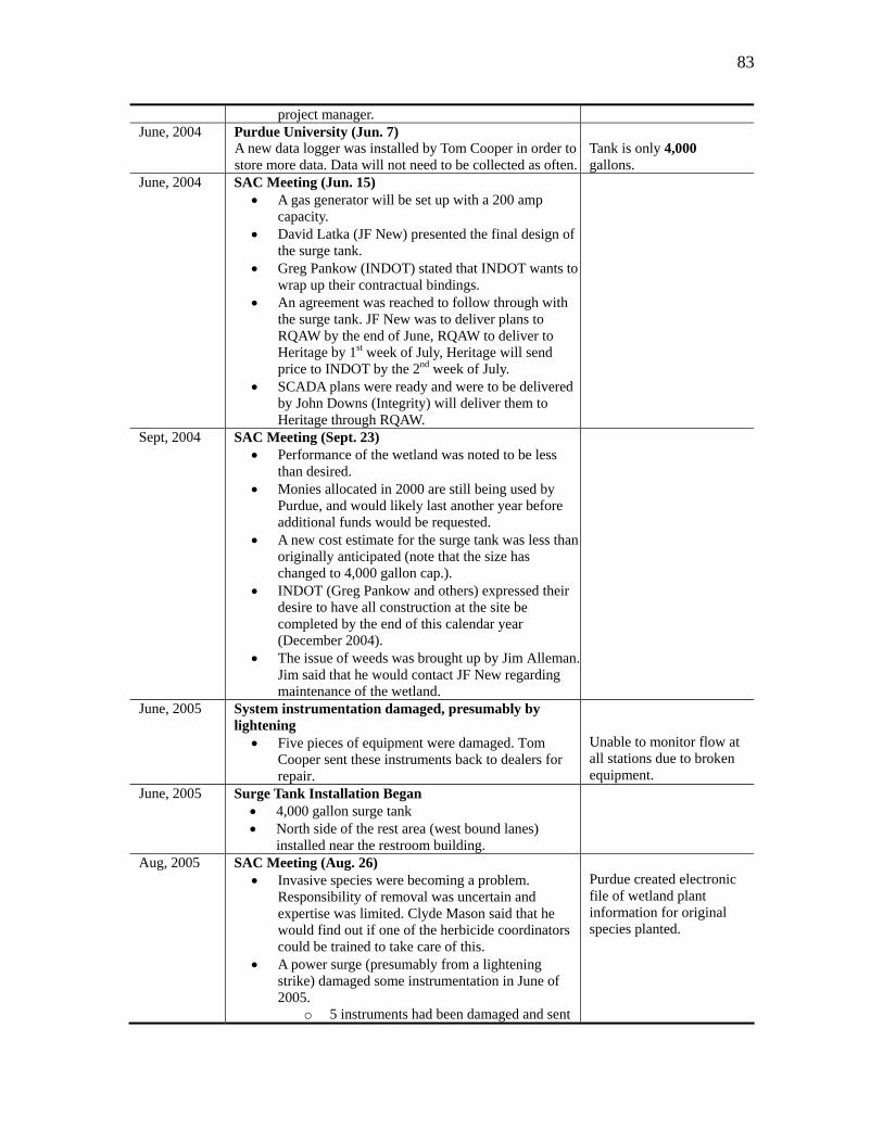
83
project manager. June, 2004 Purdue University (Jun. 7)
A new data logger was installed by Tom Cooper in order to store more data. Data will not need to be collected as often.
Tank is only 4,000 gallons.
June, 2004 SAC Meeting (Jun. 15) • A gas generator will be set up with a 200 amp
capacity. • David Latka (JF New) presented the final design of
the surge tank. • Greg Pankow (INDOT) stated that INDOT wants to
wrap up their contractual bindings. • An agreement was reached to follow through with
the surge tank. JF New was to deliver plans to RQAW by the end of June, RQAW to deliver to Heritage by 1st week of July, Heritage will send price to INDOT by the 2nd week of July.
• SCADA plans were ready and were to be delivered by John Downs (Integrity) will deliver them to Heritage through RQAW.
Sept, 2004 SAC Meeting (Sept. 23) • Performance of the wetland was noted to be less
than desired. • Monies allocated in 2000 are still being used by
Purdue, and would likely last another year before additional funds would be requested.
• A new cost estimate for the surge tank was less than originally anticipated (note that the size has changed to 4,000 gallon cap.).
• INDOT (Greg Pankow and others) expressed their desire to have all construction at the site be completed by the end of this calendar year (December 2004).
• The issue of weeds was brought up by Jim Alleman.Jim said that he would contact JF New regarding maintenance of the wetland.
June, 2005 System instrumentation damaged, presumably by lightening
• Five pieces of equipment were damaged. Tom Cooper sent these instruments back to dealers for repair.
Unable to monitor flow at all stations due to broken equipment.
June, 2005 Surge Tank Installation Began • 4,000 gallon surge tank • North side of the rest area (west bound lanes)
installed near the restroom building.
Aug, 2005 SAC Meeting (Aug. 26) • Invasive species were becoming a problem.
Responsibility of removal was uncertain and expertise was limited. Clyde Mason said that he would find out if one of the herbicide coordinators could be trained to take care of this.
• A power surge (presumably from a lightening strike) damaged some instrumentation in June of 2005.
o 5 instruments had been damaged and sent
Purdue created electronic file of wetland plant information for original species planted.

84
back to dealers for repair. o The instruments have since arrived and
will be reinstalled. • Tom Duncan said he would find out more about the
status of the SCADA system over the next week. • INDOT (Greg Pankow) expressed concern that
there had been no representative from FHWA in the past several meetings.
• Effluent quality was reported by Purdue: o High percentage removal in wetland cells.o Surface discharge standards are not yet
met, but the water may qualify for discharge to the city without surcharges.
• Biofield sampling is to be conducted in the future.• INDOT (Greg Pankow) stated that the project needs
to be closed soon. SCADA and generator still have not been paid for.
• Steve Land informed the group that there was a possibility of the first septic tank might have developed a crack; it may need repair.
Aug, 2005 Surge Tank Installation Completed • Presumably, flow restored to wetland through the
storage tank.
Feb, 2006 SAC Meeting (Feb. 24) • Presumably, the current state of the wetland was
discussed. o The wetland plant species in all cells were
affected by the surge tank installation where flow was restricted to the wetland system.
o Many plant species are no longer present, and the remaining plants appear to be dying.
o A vast amount of invasive species (weeds) are present in the cells.
• Presumably, JF New will decide whether or not to replant the wetland cells based on the wetland species’ ability to re-grow.
May, 2006 Wetland Cells replanted • Clyde Mason replanted all of the wetland cells with
a number of plants. After observation it was noted that not all original plant species were replanted, only a select few.
June, 2006 SAC Meeting (Jun. 7) • Presumably, water effluent quality was discussed. • A downward trend was noted in effluent quality.
TSS, NH3, and BOD removal have been decreased, possibly due to inconsistent flow to the wetlands, which may have caused the plants to die and decrease in quantity, thus causing the decreased removal.
o A possible need to replant the wetland cells may be justified.
• Presumably, water flow data was discussed. o There are gaps in the flow data.

85
• Equipment failure after the presumed lightening strike.
• The data logger was unplugged during surge tank construction and SCADA system installation.
• There are inherent measurement problems with the instruments.
o Rebeka Sultana has developed a hydraulic model of the wetland system.
• The SCADA system was discussed. o Data since January 2006 was in question
as to who had it and how it could be accessed.
o A training schedule for the SCADA system is needed.
o Web access of the system and/or data – is this possible?
• Recycle pumps are not working as of May 22, 2006.
• Data from the biofield was discussed. o Samples are only available from the
deepest well. o Samples show that treatment is not as
desired and flow to the biofield should be shut off.
• Data availability was discussed. Should raw data be put on a website or is data presented at meetings enough detail?