DIVISION OF THE HUMANITIES AND SOCIAL SCIENCES

CALIFORNIA INSTITUTE OF TECHNOLOGY PASADENA, CALIFORNIA 91125

AN EXPERIMENTAL STUDY OF THE CENTIPEDE GAME

Richard D. McKelvey and Thomas R. Palfrey

,... 0

0 'r

SOCIAL SCIENCE WORKING PAPER 732

May 1990 Revised August 1991

AN EXPERIMENTAL STUDY OF THE CENTIPEDE GAME

Richard D. McKelvey and Thomas R. Palfrey

Abstract

We report on a series of experiments in which individuals play a version of the centipede game. In this game, two players alternately get a chance to take the larger portion of a continually escalating pile of money. As soon a.s one person takes, the game ends with that player getting the larger portion of the pile, and the other player getting the smaller portion. If one views the experiment as a complete information game, all standard game theoretic equilibrium concepts predict the first mover should take the large pile on the first round. The experimental results show that this does not occur.

An alternative explanation for the data. can be given if we reconsider the game as a game of incomplete information in which there is some uncertainty over the payoff functions of the players. In particular, if the subjects believe there is some small likelihood that the opponent is an altruist, then in the equilibrium of this incomplete information game, players adopt mixed strategies in the early rounds of the experiment, with the probability of ta.king increasing as the pile gets larger. vVe investigate how well a version of this model explains the data observed in the centipede experiments.

AN EXPERIMENTAL STUDY OF THE CENTIPEDE GAME

Richard D. McKelvey and Thomas R. Palfrey*

1 Overview of the Experiment and the Results

This paper reports the results of severa.l experimental games for which the predictions of Nash equilibrium are widely acknowledged to be intuitively unsatisfactory. We explain the deviations from the standard predictions using an approach that combines recent developments in game theory with a parametric specification of the errors individuals might make. We construct a structural econometric model and estimate the extent to which the behavior is explainable by game-theoretic considerations. This model allows us to measure the amount of errors individuals make, and the amount of learning by subjects as they gain experience. Also, we can measure individuals' beliefs about the behavior of the other players, measure the amount of heterogeneity in those beliefs, and test whether these beliefs are consistent with the actual behavior of the other players.

In the games we investigate, the use of backward induction and/or the elimination of dominated strategies leads to a unique Nash prediction, but there are clear benefits to the players if for some reason, some players fail to behave in this fashion. Thus, we have intentionally chosen an environment in which we expect Nash equilibrium to perform at its worst. The best known example of a game in this class is the finitely repeated prisoners' dilemma. We focus on an even simpler and, we believe more compelling, example of such a game, the closely related alternating-move game that has come to be known as the "centipede game" (See Binmore (1987)).

The centipede game is-a finite move extensive form two person game in which each player alternately gets a turn to either terminate the game with a favorable payoff to itself, or continue the game, resulting in social gains for the pair. As far as we are aware,

*Support for this research was provided in part by NSF grants #IST-8513679 and #SES-878650 to the California Institute of Technology. We thank Mahmoud El-Gama! for valuable discussions concerning the econometric estimation, and we thank Richard Boylan, Mark Fey and Arthur Lupia for able research assistance. We thank the JPL-Caltech joint computing project for granting us time on the CRAY X-MP at the Jet Propulsion Laboratory. \i\Te also are grateful for comments from many seminar participants.

1

the centipede game was first introduced by Rosenthal (1982), and has subsequently been studied by Binmore (1987), Kreps (1990) and Reny (1988). The original versions of the game consisted of a sequence of a hundred moves (hence the name "centipede") with linearly increasing payoffs. More recently a concise version of the centipede game with exponentially increasing payoffs, called the "Sha.re or Quit" game, is studied by Megiddo (1986), and a slightly modified version of this game is analyzed by Aumann (1988). It is this exponential version that we study here.

In Aumann's version of the centipede game, two piles of money are on the table. One pile is larger than the other. There are two players, each of whom alternately gets a turn in which it can choose either to take the larger of the two piles of money or to pass. vVhen one player takes, the game ends, with the player whose turn it is getting the large pile and the other player getting the small pile. On the other hand, whenever a. player passes, both piles are multiplied by some fixed a.mount, and the play proceeds to the next player. There are a finite number of moves to the game, and the number is known in advance to both players. In Auma.nn's version of the game, the pot starts at $10.50, which is divided into a large pile of $10.00 and a small pile of $.50. Ea.ch time a. player passes, both piles a.re multiplied by 10. The game proceeds a total of six moves, i. e, three moves for each player.

It is easy to show that any Na.sh equilibrium to the centipede game involves the first player taking the large pile on the first move - in spite of the fact that in an eight move version of the game, both players could be multi-millionaires if they were to pass every round. Since all Na.sh equilibria. make the same outcome prediction, clearly any of the usual refinements of Na.sh equilibrium also make the same prediction. We thus have a situation where there is an unambiguous prediction made by game theory.

Despite the unambiguous prediction, game theorists have not seemed too comfortable with the above analysis of the game, wondering whether it really reflects the way in which anyone would play such a game (See e. g. Binmore (1987) and Aumann (1988)). Yet, there has been no previous experimental study of this ga.me. 1

In the simple versions of the centipede game we study, the experimental outcomes are quite different from the Na.sh predictions. To give an idea how badly the Na.sh equilibrium (or iterated elimination of dominated strategies) predicts outcomes, only 37 of 662 games encl with the first player ta.king the large pile on the first move, while 23 of the games encl with both players passing at every move! (The rest of the outcomes a.re scattered in between.) While these facts may be the most striking feature of the experiment to many readers, we believe· that the- real challenge is to come up with an internally consistent model to explain these data-a model which allows us to address Lhe issue of how badly (or perhaps how well) game theory predicts behavior in these difficult environments.

1There is related experin1ental vvork on the prisoner's dile1n1na ga1ne by Selten and Stoecker (1986) and on an ultin1atum bargaining ga1ne \vith an increasing cake by Guth et al. (1991). Also related experimental \York on inco1nplete information gan1es can be found in Ca.n1erer and \iVeigelt (1988), .Jung et al. (1989), and Neral and Ochs (1989).

2

One class of explanations for how such apparently irrational behavior could arise is based on reputation effects and incomplete information. 2 This is the approach we adopt. The idea is that players believe there is some possibility that their opponent has payoffs different from the ones we tried to induce in the laboratory. In our game, if a player places sufficient weight in its utility function on the payoff to the opponent, the rational strategy is to always pass. Such a player is labeled an altruist. 3 If it is believed that there is some likelihood that each player may be an altruist, then it can pay a selfish player to try to mimic the behavior of an altruist in an attempt to develop a reputation for passing. These incentives to mimic are very powerful, in the sense that a very small belief that altruists are in the subject pool can generate a lot of mimicking, even with a very short horizon.

The structure of the centipede game we run is sufficiently simple that we can solve for the equilibrium of a parametrized version of this reputational model. Using standard maximum likelihood techniques we can then fit this model. Despite the assumption of only a single kind of deviation from the "selfish" payoffs normally assumed in induced­value theory4 we are able to fit the data remarkably well, and obtain an estimate of the proportion of selfish players on the order of 95 percent of the subject pool. In addition to estimating the proportion of altruists in the subject pool, we also estimate the beliefs of the players about this proportion. Surprisingly, we find that subjects' beliefs are, on average, equal to the estimated "true" proportion of altruists, thus providing evidence in favor of a strong version of rational expectations. We also estimate a decision error rate to be on the order of 5%-10% for inexperienced subjects and roughly half that for experienced subjects, indicating two things: 1) a significant amount of learning is taking place, and 2) even with inexperienced subjects, only a small fraction of their behavior is unaccounted for by a simple game-theoretic equilibrium model in which beliefs are accurate.

Our experiments can be compared to those of Camerer and Weigelt (1988). In our experiments, we find that we can explain the data only if we assume that there is a belief that a certain percentage of the subjects in the population are altruists. This is equivalent to asserting that subjects did not believe that the utility functions we attempted to induce are the same as the utility functions that all subjects really use for making their decisions. I. e., subjects have their own personal beliefs about parameters of the experimental design that are at odds with those of the experimental design. This is very similar to the finding in Camerer and \"leigelt, who found that one way to account for behavior in their experiments was to introduce "homemade priors" -i.e., beliefs that there were more subjects who always act cooperatively similar to our (altruists) than were actually induced to be so in their experimental design. (They used a rule-of-thumb procedure to obtain a homemade prior point estimate of 17%.) Our analysis differs from

2See Kreps and Wilson (1982a), Kreps et al. (1982), Fudenberg and Maskin (1986), and Kreps (1990) pp. 536-543.

3 '¥e called them "irrationals" in an earlier version of the paper. The equilibriu1n implications of this kind of altruism has been explored in a. different kind of experin1ental gan1e by Palfrey and Rosenthal (1988). See also Cooper et al. (1990).

4 See Smith (1976).

3

Ca.merer and Weigelt partly in that we expand on this notion and integrate it into a. structural econometric model, which we then estimate using classical techniques. This enables us to estimate the number of subjects that actually behave in such a. fashion, and to address the question a.s to whether the beliefs of subjects a.re consistent.

Our experiments can also be compared to the literature on repeated prisoner's dilem­mas. This literature (see eg., Selten and Stoecker (1986) for a review) finds that expe­rienced subjects exhibit a pattern of "tacit cooperation' until shortly before the end of the game, when they start to adopt non-cooperative behavior. Such behavior would be predicted by incomplete information models like that of Kreps et al (1982). However, Selten and Stoecker also find that inexperienced subjects do not immediately adopt this pattern of play, but that it takes them some time to "learn to cooperate." Selten and Stoecker develop a learning theory model that is not based on optimizing behavior to account for such a learning phase. One could alternatively develop a. model similar to the one used here, where in addition to incomplete information a.bout the payoffs of others, all subjects have some cha.nee of ma.king errors, which decreases over time. If some other subjects might be ma.king errors, then it could be in the interest of all subjects to take some time to learn to cooperate, since they can masquerade as slow learners. Thus, a natural analog of the model used here might offer an alternative explanation for the data in Selten and Stoecker.

2 Experiments

Our budget is too constrained to use the payoffs proposed by Aumann. So we run a rather more modest version of the centipede game. In our laboratory games, we start with a total pot of $.50 divided into a. large pile of $.40 and a. small pile of $.10. Ea.ch time a player passes, both piles a.re multiplied by two. We consider both a two round (four move) and a three round (six move) version of the game. This lea.els to the extensive forms illustrated in Figures 1 and 2. In a.clclition, we consider a version of the four move game in which all payoffs a.re quadrupled. This "high payoff" experiment therefore produced a payoff structure equivalent to the last four moves of the six move game.

In each experimental session we used a total of twenty subjects. The subjects were divided into two groups a.t the beginning of the experiment, which we ca.lied the Reel and the Blue groups. In each game, the Reel player was the first mover, and the Blue player was the second mover. Ea.ch subject then participated in ten games, one with ea.ch of the subj eds in thecother group. 5 .· The experiments were all conducted through computer terminals. Subjects did not communicate with other subjects except through the strategy choices they ma.de. Before each game, ea.ch subject was matched with another subject, of the opposite color, with whom they had not been previously matched, and then the

50nly one of the three versions of the ga.111e \Vas played in a given session. In Experin1ents 2 and 6, not all subjects showed up for the experi1nent, so there \Vere only 18 subjects 1 \vith 9 in each group 1 and consequently each subject played only 9 ga1nes.

.40

.10

.40

.10 .20 .80

1.60 .40

.80 3.20

p 6.40 1.60

Figure 1: The Four Move Centipede Game.

.20

.80 1.60

.40 .80

3.20 6.40 1.60

3.20 12.80

Figure 2: The Six Move Centipede Game.

p 25.60

6.40

subjects who were matched with each other played the game in either Figure 1 or Figure 2 depending on the experiment.

All details described above were made common knowledge to the players, at least as much as is possible in a laboratory setting. For example, the instructions were read to the subjects with everyone in the same room (See Appendix A for the exact instructions read to the subjects). Thus it was common knowledge that no subject was ever matched with any other subject more than once. In fact we used a rotating matching scheme which insures that no player i ever plays against a player who has previously played someone who has played someone that i has already played. (Further, for any positive integer n, the sentence which replaces the phrase "who has previously played someone who has played someone" in the previous sentence with n copies of the same phrase is also true). In principle, this matching scheme should eliminate potential supergame or cooperative behavior, yet at the same time allow us to obtain multiple observations on each individual's behavior.

We conducted.11 total of seven sessions( see Table 1.) Our subjects were students from Pasadena Community College (PCC) and from the California Institute of Technology (CIT). No subject was used in more than one session. Sessions 1-3 involved the regular four move version of the game, session 4 involved the high payoff four move game, and session 5-7 involved the six move version of the game. This gives us a total of 58 subjects and 281 plays of on the four move game, and 58 subjects with 281 plays of on the six move game, and 20 subjects with 100 plays of the high payoff game. Subjects were paid in cash the cumulative a.mount that they earned in the experiment plus a fixed amount

5

for showing up($ 3.00 for CIT students and$ 5.00 for PCC students).6

Session 1 Subject

# Pool 1 PCC 2 PCC 3 CIT 4 CIT 5 CIT 6 PCC 7 PCC

# games/ total# subjects subject games

20 10 100 18 9 81 20 10 100 20 10 100 20 10 100 18 9 81 20 10 100

Table 1 Experimental Design

3 Descriptive Summary of Data

# High moves Payoffs

4 No 4 No 4 No 4 Yes 6 No 6 No 6 No

The data from the experiment is given in Appendix C. In Table 2, we present some simple descriptive statistics summarizing the behavior of the subjects in our experiment. Table 2a gives the raw outcomes for

the experiment, indicating how many games end a.t each of the terminal outcomes. Thus ni is the number of games ending after the ;th move i. e., with the subject who chooses TAKE at node i. Table 2b gives the implied probabilities, Pi of ta.king a.t the ;th

decision node of the game conditional on having reached that node. In other words, Pi is the proportion of games among those that reached node i, in which the subject who moves a.t node i chose TAKE. Thus, in a game with rn decision nodes, p; = 2.:"~+ 1 .

J=i n;

All standard game theoretic solutions (Na.sh equilibrium, iterated elimination of dom­inated strategies, maximin, rationalizability, etc.,) would predict Pi = 1 for all 1 S: i S: m. The weaker requirement of rationality that subjects not adopt dominated strategies would predict that Pm = l. As is evident from the table, we can reject out of hand either of these hypotheses of rationality. In only 73 of the four move games, 13 of the six move games and 153 of the high payoff games does the first mover choose TAKE on the first round. So the.subjects dearly·do not iteratively eliminate dominated strategies. Further, when the experiment reaches the last move, the player with the last move adopts the dominated strategy of choosing PASS roughly 253 of the time in the four move games7

153 in the six move games, and 313 in the high payoff games.

6The stakes in these ga.111es ¥-7ere very large by usual standards. Students earned fro1n a low of$ 7 .00 to a. high of$ 75.00, in sessions that averaged less than 1 hour - average earnings were $ 20.50 ($ 13.40 in the four inove, $ 30.77 in the six 111ove, and$ 41.50 in the high payoff four move version).

7It should be noted that 7 of the 14 cases in this category are attributable to two of the 29 subjects.

6

Session 111 112 113 114

1 Four 2 Moves 3

Total High Payoff 4 Six 5 Moves 6

7

Total

Session 1 (PCC)

Four 2 (PCC) Move

3 (CIT)

Total 1-3

High 4 (CIT) Payoff

5 (CIT)

Six 6 (PCC) Move

7 (PCC)

Total 5-7

(PCC) 6 26 44 20 (PCC) 8 31 32 9 (CIT) 6 43 28 14

20 100 104 43 (CIT) 15 37 32 (CIT) 2 9 39 (PCC) 0 2 3 (PCC) 0 7 14

2 18 56

Table 2a Raw Outcomes

P1 P2 p3 .06 .28 .65 (100) (94) (68) .10 .42 .76 (81) (73) ( 42) .06 .46 .55 (100) (94) (51) .07 .38 .65 (281) (261) (161) .15 .44 .67 (100) (85) ( 48)

.02 .09 .44 (100) (98) (89) .00 .02 .04 (81) (81) (79) .00 .07 .15 (100) (100) (93) .01 .06 .21 (281) (279) (261)

Table 2ba Implied Probabilities

for the Centipede Ga.me

11 28 37 43

108

p4 .83 (2L1) .90 (10) .61 (23) .75 (57) .69 (16)

.56 (50) .49 (76) .54 (79) .53 (205)

115 116 n1

4 1 9

14 5 20 1 1 28 9 2 23 12 1

71 22 4

Ps P6

.91 .50 (22) (2) .72 .82 (39) (11) .64 .92 (36) (13) .73 .85 (97) (26)

aThe number in parenthesis is the nun1ber of observations in the ga1ne at that node.

7

Game 111

Four Move 20 (Exp #1-3) 1-5 9 6-10 11 Six Move 0 (Exp #5-7) 1-5 0 6-10 2

Game Pt Four Move .07 (Exp #1-3) (281) 1-5 .06

(145) 6-10 .08

(136) Six Move .01 (Exp #5- 7) (281) 1-5 .00

(145) 6-10 .01

(136)

112 113 114 115

100 104 43 14

44 52 29 11 56 52 14 3 18 56 108 71

8 25 48 10 31 60

Table 3a Raw Outcomes

P2 p3 .38 .65 (261) (161) .32 .57 (136) (92) .49 .75 (125) (69) .06 .21 (279) (261) .06 .18 (145) (137) .07 .25 (134) (124)

Table 3b

48 23

p4 .75 (57) .75 ( 40) .82 (17) .53 (205) .43 (112) .65 (93)

116

22

13 9

Ps

.73 (97) .75 (64) .70 (33)

Implied Mixed Strategies Comparison of early versus late plays

in the low pa.yoff centipede game

8

117

4

3 1

PB

.85 (26) .81 (16) .90 (10)

The most obvious and consistent pattern in the data is that in all of the experiments, the probability of taking increases as we get closer to the last move (see Table 2b ). The only exception to this pattern is in Experiment 5 (CIT) in the last two moves, where the probabilities drop from .91 to .50. But here the figure at the last move is based on only two observations. Thus any model which we use to explain the data should make this basic prediction. In addition to this dominant feature, there are some less obvious patterns of the data, which we now discuss.

Table 3 indicates that there are some differences between the earlier and later plays of the game in a given treatment which are supportive of the proposition that as subjects gain more experience with the game, their behavior appears "more rational." Recall that with the matching scheme we use, there is no reason to expect players to play any differently in earlier games than in later games. Table 3 shows that in both the four and six move experiments, subjects chose TAKE with higher probability at all stages of the game (with the exception of node 5 of the six move games). Further, the number of subjects that adopt the dominated strategy of passing on the last move drops to 4 of 27, or 15%.

There is at least one other interesting pattern in the data. Specifically, if we look at individual level data, there are several subjects who PASS at every opportunity they have.8 Vve call such subjects altruists, because an obvious way to rationalize their behav­ior is to assume that they have a utility function that is monotonically increasing in the sum of the reel and blue payoffs, rather than a. selfish utility function that only depends on that players' own payoff. Overall, there were a total of 9 players who chose PASS at every opportunity. Roughly half (5) of these were reel players and half (5) were in 4-move games. At the other extreme (i.e. the Nash equilibrium prediction), only 1 out of a.ll 138 subjects chose TAKE at every opportunity. This indicates the strong possibility that players who will always choose PASS do exist in our subject pool, and also suggests that a theory which successfully accounts for the data will almost certainly have to admit the existence of a.t lea.st a small fraction such subjects.

Finally, there are interesting non-patterns in the data. Specifically, unlike the ten cases cited above, the preponderance of the subject behavior is inconsistent with the use of a single pure strategy throughout all ga.rnes they played. For example, subject #8 in experiment #1 (a. red player) chooses TAKE at the first chance in the second game it participates in, then PASS at both opportunities in the next game, PASS at both opportunities in the fourth game, TAKE at the first chance in the fifth game, and PASS at the first chance in the sixth game. Fairly common irregularities of this sort, which appear rather haphazard from a casual gla.nce, would seem to require some degree of randomness to explain. \"lhile some of this behavior may indicate evidence of the use of mixed strategies, some such behavior is impossible to rationalize, even by resorting to the possibility of altruistic individuals or Bayesian updating across games. For example, subject #16 in experiment #1 (a. blue player), chooses PASS at the la.st node of the

8Some of these subjects had as n1any as 24 opportunities to TAJ(E in the 10 ga.1nes they played! See Appendix C.

9

first game, but takes at the first opportunity a few games later. Rationalization of this subject's behavior as altruistic in the first game is contradicted by the subject's behavior in the later game. Rational play cannot account for some sequences of plays we observe in the data, even with a model that admits the possibility of a.ltruistic players.

4 The Model

In what follows, we construct a structural econometric model based on the theory of games of incomplete information that is simultaneously consistent with the experimental design and the underlying theory. Standard maximum likelihood techniques ca.n then be applied to estimate the underlying structural parameters.

The model we construct consists of an underlying incomplete information game to­gether with a specification of two sources of errors ~ errors in actions a.nd errors in beliefs. The model is constructed to account for both the time-series nature of our data and for the dependence a.cross observations, features of the data set that derive from a design in which every subject plays a sequence of games against different opponents. The model is able to account for the broad descriptive findings summarized in the pre­vious section. By parametrizing the structure of the errors, we can also address issues of whether there is learning going on over time, whether there is heterogeneity in beliefs, and whether individua.ls' beliefs are "rational".

We first describe the basic model, and then describe the two sources of errors.

4.1 The Basic Model

If, as appears to be the case, there are a substantial number of altruists in our subject pool, it seems reasonable to assume that the possible existence of such individuals is commonly known by all subjects. Our basic model is thus a game of two sided incomplete information where each individual can be one of two types (selfish or altruistic), and there is incomplete information about the number of altruists in the population.

In our model, a selfish individual is defined as an individual who derives utility only from its own payoff, and acts to maximize this utility. In analogy to our definition of a selfish individual, a natural definition of an altruist would be as an individual who derives utility not only-from its own payoff, but also from the payoff of the other player. For our purposes, to avoid having to make parametric assumptions about the form of the utility functions, it is more convenient to define an altruist in terms of the strategy choice rather than in terms of the utility function. Thus, we define an altruist as an individual who always chooses PASS. However, it is important to note that we could obtain an equivalent model by making parametric assumptions on the form of the utility functions. For example, if we were to assume that the utility to player i is a convex combination of its own payoff and tha.t of its opponent, then any individual who places

10

a weight of at least ~ on the payoff of the opponent has a dominant strategy to choose PASS in every round of the experiment. Thus, defining altruists to be individuals who satisfy this condition would lead to equivalent behavior for the altruists.

The extensive form of the basic model for the case when the probability of a. selfish individual equals q is shown in Figure 3. This is a standard game of incomplete informa­tion. There is an initial move by nature in which the types of both players a.re drawn. If a player is altruistic, then the player has a. trivia.I strategy choice (namely, it can PASS). If a. player is selfish, then it can choose either PASS or TAKE.

Player Player Player Player Player Player Player Player 1 2 1 2 1 n-2 n-1 n

! ! ! ! ! ! ! ! (1-q) 2 fa>----=p~~lt--=p~~.-~~p~~lt--=p~~-----,p,,-- • • • p~ p

q(l-q)

q(l-q)

/ / / / / / / / / / I I I I I I I I I I I I I I I I I I I I ' I ' I ' ' ' '

IP ' p

' I I I

T I I I I I

I az I ' b2

'

' ' T I I I I I

p p • • •

/ / I I I I I I

/ / I I I I ' '

I ' P I ' I T I I I I a I I n-2 I ' bn-2 I '

/ / I I I I I

' ' T I I I I I

p

' ' I p IP

I , P IP , P

' I '

• • • IP , P IP I ' I

I a

1 I

bl )

I I I I

/

I I I I I I I I I I I I

I a I I I bn-1 I I

a3

I I a I I I 5 I

b3 / / b5 / / n)/ /

r: , r: , r: , r: , r: • • • p

Figure 3: Centipede Game with Incomplete Information Dashed lines represent information sets and open

circles are starting nodes, with probabilities indicated.

4.1.1 Equilibrium of the Basic Model

p

Most of the formal analysis of the equilibrium appears in an appendix, but it is instruc­tive to provide a brief overview of the equilibrium strategies, and to summarize how

11

equilibrium strategies vary over the family of games indexed by E and q. We ana1ytically derive in the appendix the solution to the N-move game with E = 0, for arbitrary values of q (the common knowledge belief that a randomly selected player is an altruist) ranging from 0 to 1.

Given a level of altruism q, a strategy for the first player in a six move game is a vector, (p1,p3,p5), where Pi specifies the probability that RED chooses TAKE on move i conditional on RED being a selfish player. Similarly, a strategy for BLUE is a vector (pz,p4,p5) giving the probability that BLUE chooses TAKE on the corresponding move conditional that BLUE is selfish. Thus a strategy pair is a vector p = (p,,p2 , ... ,p6 ),

where the odd components are moves by RED and the even components are moves by BLUE. Similar notation is used for the four move game.

In Appendix A, we prove that there is a unique sequential equilibrium to the game, and solve for this equilibrium as a function of q. Let us write p( q) for the solution as a function of q. From the solution, we can compute the implied probabilities of choosing TAKE at each move, and the probability s(q) = (s 1 (q), ... ,s7(q)) of observing each of the possible outcomes, T, PT, PPT, PPPT, PPPPT, PPPPPT, PPPPPP. Thus, s1 (q) = qp1 (q), s2(q) = q2(1- p1(q))p2(q) + q(l - q)p2(q), etc. Figures 4 and 5 illustrate the probability of choosing TAKE at each node for the four and six move games respectively, and Figures 6 and 7 give the probabilities of the outcomes as a function of q.

The derivation of these strategies proceeds by verifying some properties of the equi­librium.

Property 1: For any q, in any equilibrium, BLUE assigns 0 probability of choosing PASS on its last move.

Property 2: If q = 0, the (essentially) unique equilibrium is for both RED and BLUE players to always choose TAKE.

Property 3: If q > ~, the unique equilibrium is for both players to always choose PASS, except on the last move, when BLUE chooses TAKE.

Property 4. If q E (0, ~) then there is no pure strategy equilibrium, but there does exist an equilibrium in mixed strategies.

It follows from the properties of the solution that the equilibrium predictions of game theory are extremely sensitive to the beliefs that players have about the proportion of altruists in the population. The basic intuition of what is going on is well-summarized in the literature on signalling and reputation building (for example, Kreps and Wilson (1982b), Kreps et al. (1982)) and is exposited very nicely for a one-sided incomplete information version of the centipede game more recently in Kreps (1990).

The guiding principle is very easy to understand, even if one cannot follow the technical details of the appendix. Because of the uncertainty in the game when it is not common knowledge that everyone is self-interested, it will generally be worthwhile for a selfish

12

p r..:I. tall.••

0 ••

0.'

0.4

0.2

p blue take•

Four move•, both type•

Four mov••• both type•

ep•ilon .. o

r=-:i L_j

epailon•O

o.•J~-------0 ••

0.4

0.2

r=-:i L_j

Figure 4: Implied Probabilities for Four Move Game.

13

p red takll•

0. I

0.6

o.•

[] ' 5

0.2

p bll.le t.ak••

Six 111ov••• both type•

o .• ~---------0 ••

o.• [] •

•

0.2

Figure 5: Implied probabilities for Six Move Game.

14

p of out=-•

0.0

0.6

0 ••

o .•

0 ••

0 ••

0.2

Four fftOvt•, both typ••

--------"~=====:~~========~-~:-------------

i

I I I J

0.05 0.1

---·····-·--··--·-----

I 0.15

,, "' "'' ---- pppp

I q 0.2

Figure 6: Outcome Probabilities for Four Move Game

epeilon•O

-----------------------------'~'-, , _______ :_:_._

..... -------- pppt ••• ---- ppppt

·········........ :::::::::::::::::.

'········ ... ••••• I

IJ..--X-~---+-------..... ------~'~'c...,,__ ______ ...... 0.05 0.1 o.1s 0 .2

Figure 7: Outcome Probabilities for Six Move Game

15

player to mimic altruistic behavior, in order to confuse the opponent as to whether or not it is an altruist. This is not terribly different from the fact that in poker it may be a good idea to bluff some of the time in order to confuse your opponent about whether or not you have a good hand. In our games, for any amount of uncertainty of this sort, equilibrium will involve some degree of imitation. The form of the imitation in our setting is obvious: selfish players sometimes pass, to mimic an altruist. By imitating an altruist one might trick an opponent into passing, thereby raising one's final payoff in the game. The amount of imitation depends directly on the beliefs about the likelihood of a randomly selected player being an altruist. The more likely players believe there are altruists in the population, the more imitation there is. In fact, if these beliefs are sufficiently high (at least ~, in our versions of the centipede game), then selfish players will always imitate altruists, thereby completely reversing the predictions of game theory when it is common knowledge that there are no altruists. Between 0 and ~, the theory predicts the use of mixed strategies by self-interested players.

4.1.2 Limitations of the Basic Model

The primary observation to make from the solution to the basic model is that this model can account for the main feature of the data noted in the previous section - namely that probabilities of taking increase as the game progresses. For any level of altruism above .f, in the four move game, and for any value above ./, in the six move game, the solution satisfies the property that Pi ~ Pi whenever i > j.

Despite the fact that the basic model accounts for the ma.in pattern in the data, it is just as obvious that the basic model cannot account for the remaining features of the data. It is apparent from Figures 6 and 7 that for any value of q, there is at least one outcome with a 0 or close to 0 probability of occurrence. So the model will fit poorly data in which all of the possible outcomes occur. Nor can it account for any consistent patterns of learning in the data, or some of the irregularities described earlier.

To account for these features of the data, we introduce two additionaI elements to the model - the possibility of errors in actions, and the possibility of errors in beliefs.

4.2 Errors in Actions ~ Noisy Play

One explanation of the apparently bizarre irregularities that we noted in the previous section is that players may "experiment" with different strategies in order to see what happens. Alternatively, subjects may simply "goof", either by pressing the wrong key, or by accidentally confusing which color player they a.re, or by failing to notice that it is the la.st round, or some other random event. Lacking a good theory for how and why this experimentation or goofing takes place, a natural way to model it is simply as noise. So we refer to it as noisy play.

16

We model noisy play in the following way. In game t, at node s, if p* is the equilibrium probability of TAKE that the player at that node attempts to implement, we assume that the player actually chooses TAKE with probability (1 - e,)p*, and makes a random move (i.e. TAKES or PASSES with probability .5) with probability e,. Therefore, we can view -',f as the probability that a player experiments, or, alternatively, goofs in the t'h game played. We call e, the error rate in game t. We assume that both types (selfish and altruistic) of players make errors at this rate at all nodes of game t, and that this is common knowledge among the players.

4.2.1 Learning

If the reasons for noisy play are along the lines just suggested, then it is natural to believe that the incidence of such noisy play will decline with experience. For one thing, as experience accumulates, the informational value of experimenting with alternative strategies declines, as subjects gather information about how other subjects are likely to behave. Perhaps more to the point, the informational value will decline over the course of the 10 games a subject plays simply because, as the horizon becomes nearer, there are fewer and fewer games where the information accumulated by experimentation can be capitalized on. For different, but perhaps more obvious reasons, the likelihood that a subject will goof is likely to decline with experience. Such a decline is indicated in a wide range of experimental data in economics and psychology, spanning many different kinds of tasks and environments. Vve call this decline learning.

We assume a particular parametric form for the error rate as a function of t. Specifi­cally, we assume that individuals follow an exponential learning curve. The initial error rate is denoted by e and the lea.ming pa.rameter is 5. Therefore,

Notice that, while according to this specification the error rate may be different for different t, it is assumed to be the same for a.II individuals, and the same at a.II nodes of the game. More complicated specifications a.re possible, but we suspect that such parameter proliferation would be unlikely to shed much more light on the data. \Nhen solving for the equilibrium of the game, we assume that players are aware that they experiment (or might goof) and learn, and are a.ware that other players experiment (or goof) and learn too. 9 Formally, when solving for the Bayesian equilibrium TAKE probabilities, we assume that E and 8 a.1-e conHnBn knowledge.

9 An alternative specification 'vould have subjects being a\.vare that others experiment and goof, but act as if they do not make these "errors." Such a n1odel is analytically more tractable and leads to very similar conclusions, but see1ns less appealing on theoretical grounds.

17

4.2.2 Equilibrium with errors in actions

For e > 0, we do not have an a.na1ytica.I solution for the equilibrium. The solutions were numerically calculated using GAMBIT, a computer algorithm for calculating equilibrium strategies to incomplete information games, developed by McKelvey (1990). For compar­ison, the equilibrium strategies as a. function of q, for e = .2 a.re illustrated graphically in Figures 8 to 11. These figures ca.n be com pa.red to Figures 4 to 7. Figures 8 and 9 illustrate the probability of choosing TAKE a.t at ea.ch node for the four and six move games respectively, and Figures 10 and 11 give the probabilities of the outcomes a.s a. function of q.

4.3 Errors in Beliefs - Heterogeneous Beliefs

In addition to assuming tha.t individuals can ma.ke errors in their strategies, we also assume tha.t there ca.n be errors in their beliefs. Thus, we assume that there is a true probability Q that individuals are selfish (yielding probability 1- Q of altruists), but tha.t each individual has a belief, q; of the likelihood of selfish players, which ma.y be different than the true Q rn

In particular individuals' beliefs can differ from ea.ch other, giving rise to heterogeneous beliefs.

For individual i, denote by q; the belief individual i holds that a randomly selected opponent is selfish. We assume that ea.ch incliviclua.l maintains its belief throughout all 10 games that it plays. Because this converts the simple centipede game into a. Bayesian game, it is necessary to make some kind of assumption about the beliefs a. player ha.s a.bout its opponent's beliefs, etc. etc. If there were no heterogeneity in beliefs, so tha.t q; = q for a.II i, then one possibility is that a player's beliefs a.re correct - that is, q is common knowledge, a.nd q = Q. We ca.II this rational expectations. One can then solve for the Bayesian equilibrium of the game played in a session (which is unique), as a function of e, fi, t, and q. An analytical solution is derived in Appendix A for the case of e = 0

To allow for heterogeneity, we make a para.metric assumption that the beliefs of the individuals a.re independently drawn from a Beta distribution with para.meters (o, /3), where the mean of the distribution, q, is simply equal to a~/3· There a.re several ways to specify higher order beliefs. One possibility is to assume it is common knowledge among the players that be1iefs are independently drawn from a Beta distribution with parameters ( o, (3) and that the pair ( o, (3) is also common knowledge among the players. This version of a "rational expectations" model of higher order beliefs lea.els to serious computational problems when numerically solving for the equilibrium strategies. Instead,

10This is related to the idea of homemade priors proposed by Camerer and Weigelt (1988), where they posit that subjects' beliefs about the distribution of types may differ from the distribution of types announced in the instructions of the experin1ent.

18

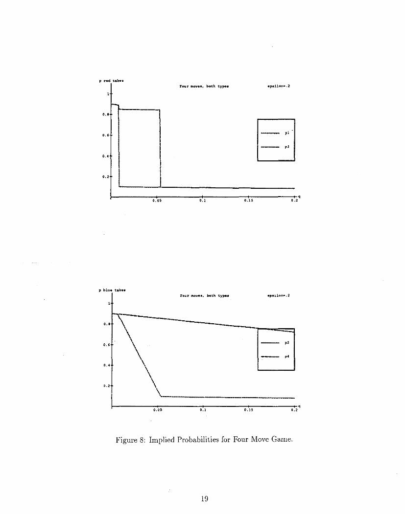
p red tak••

FO\I r 1110ve•, bot.h type• •p•ilon• .2

-0 .• ~

0 •• pl

pJ

o .•

0 .2

p blue tak•• Four mov••, both type• •p•ilon ... 2

0 •• '\ 0 .• \ p2

,. o .• \

\ .., \

\ q

0. 05 0.1 0 .15 0.2

Figure 8: Implied Probabilities for Four Move Game.

19

p red take•

Si• ,....,...., both tyr• ep•il.on ... 2

0.'

0 ••

0.4

0.2

0.005 0.01 0. 015 0. 02 0 .025 0.03

p blue. take•

Six move•, both type• epsilon•. 2

\ ---..._ ... __ ------[]------

0 ••

o.'

0 ••

0.'

Figure 9: Implied probabilities for Six Move Game.

20

p of 01.1tc:ome•

Four movee, both type• ep•ilon•.2

0.1

O.• ,,

\ -pp pt

o .. t \ , __ --_---PPPP

0.211------~ \::-1~-----:-<1-:-------+1-------+-1' 0.05 C.l 0.15 0.2

Figure 10: Outcome Probabilities for Four Move Game

p of outc:olftee

Sil( ll'ICIVe8, both typee epeilon•.2

0.8

,-r------- I . --~:'---------------~::::::::::::::; \ !

\

...... \'·... ! p~ l ---------- ::ptt

••• ,t ----- ppppt I "-.. 1 ---pppppl

I ....... L----------------------=~:::. ·. \ "·--------------------------------.-----------------------------------

0 ••

0 ••

0.2 t ____ ~-~------·--~·~~--~~--

Figure 11: Outcome Probabilities for Six Move Game

21

we use a simpler11 version of the higher order beliefs, which might be called an egotism model. Each player plays the game as if it were common knowledge that the opponent had the same belief. In other words, while we, the econometricians, assume there is heterogeneity in beliefs, we solve the game in which the players do have heterogeneous beliefs, but believe that everyone's beliefs are alike. This enables us to use the same basic techniques in solving for the Bayesian equilibrium strategies for players with different beliefs that one would use if there were homogeneous beliefs. \Ve can then investigate a weaker form of rational expectations: is the average belief equal to the true proportion f lt > • t ? (' . " - Q?) 0 a IUIS S. Le. IS a+/3 - .

Given the assumptions that we made regarding the form of the heterogeneity in beliefs, the introduction of errors in beliefs does not cha.nge the computation of the equilibrium for a given individual. It only changes the aggregate behavior we will expect to see over a. group of individuals. For example, at a.n error ra.te of Et = .2, a.nd parameters a, f3 for the Beta. distribution, we will expect to see aggregate behavior in period t which is the average of the behavior generated by the solutions in Figure 11, when we integrate out q with respect to the Beta. distribution B(a, (3).

5 Maximum Likelihood Estimation of (ex, f3, Q, E, 5)

5.1 Derivation of the Likelihood Function

Consider the version of the game where a player draws belief q. For every t, and for every Et, and for each of tha.t player's decision nodes, v, the equilibrium solution derived in the previous section yields a probability that the decision a.t tha.t node will be TAKE, condi­tional on the pla.yer a.t tha.t decision node being selfish, and conditional on that player not

ma.king an error. Denote that probability p,(e,, q, v). Therefore, the probability that a selfish type of that player would TAKE at 11 is equal to P, (Et, q, v) = % + ( 1- % )p, (Et, q, JJ J, and the probability tha.t a.n altruistic type of this player would tak~ is Pa(~,, q, v) = ~· For each individual, we observe a. collection of decisions tha.t a.re ma.de a.t all nodes reached in all ga.mes pla.yed by that player. Let N,; denote the set of decision nodes visited by player i in the t'h game played by i, and let Dti denote the corresponding set of deci­sions made by i a.t each of those nodes. Then, for a.ny given ( E, 5, q, v) with v E N,, we can compute P,( e,, q, JJ) from a.bove, by setting Et = Ee-S(t-l). From this we compute 1rt;(D,;; E, 5, q), the probability tha.t a. selfish i would have made decisions Dti in game t, with beliefs q, a.nd noise/learning parameters ( E, 5), and it equal the product of p,( e, q, v) over a.ll v reached by in game t. Letting D; denote the set of all decisions by player i, we define 7rf(D;; E, 5, q) to be the product of the 7rt;(Dtii e, 5, q) ta.ken over a.ll t. One ca.n similarly derive 7rf(D;; E, 5, q), the probability that an altruistic i would ha.ve ma.de that sa.me collection of decisions. Therefore, if Q is the true population parameter for the fraction of selfish players, then the likelihood of observing D;, without conditioning on

11\Vhile it is simpler, it is no less arbitrary.

22

i's type is given by:

1ri(Di; Q, E, 6, q) = Q7rf(Di; E, 6, q) + (1 - Q)7rf(Di; E, 6, q)

Finally, if q is drawn from the Beta distribution with parameters (a, [3), and density B( q; a, (3), then the likelihood of observing Di without conditioning on q is given by:

si(Di;Q,E,6,a,[3) = fo1

7r;(D;;Q,c,6,q)B(q;a,,6)dq

Therefore, the log of the likelihood function for a sample of observations, D is just

I

L(D;Q,E,6,a,(3) = Llog[si(Di;Q,E,6,a,[3)]. i=l

For any sample of observations, D, we then find the set of parameter values that maximize L. This was done by a global grid search using the Cray X-MP at the Jet Propulsion Laboratory.

5.2 Treatments and Hypotheses

Several estimations were performed. In our experimental design, there were 3 treatment variables:

(1) The length of the game (either 4-move or 6-move); (2) The size of the two piles at the beginning of the game (either high

payoff, ($1.60,$.40), or low payoff, ($.40, $.10)); (3) The subject pool (either Caltech undergraduates (CIT) or Pasadena

City College students (PCC)).

In addition to the statistical comparison of these, we were also interested in testing three other hypotheses:

(1) Rational Expectations. Is the estimated value of Q equal to the mean of the estimated distribution of priors, a~/3?

(2) Learning. Is the estimated value of 6 positive and significantly dif­ferent from O?

(3) Heterogeneity. Is the variance of the estimated distribution of priors significantly different from O?

23

5.3 Estimation Results

Table 4 reports the results from the estimations. Before reporting any statistical tests, we summarize several interesting features of the parameter estimates.

First, the mean of the distribution of beliefs about the proportion of altruists in the population in all the estimations was in the neighborhood of 5%. Second, the amount of heterogeneity of beliefs was estimated to be small in magnitude. Figures 12 and 13 graph the density function -of the estimated Beta distribution for the pooled sample of all experimental treatments for the four and six move experiments, respectively. Second, if one looks at the rational expectations estimates (which constrain fl = . 5

13 to equal Q),

~+

the constrained estimate of the Beta distribution is nearly identical to the unconstrained estimate of the Beta distribution. Consequently, the rational expectations estimates of µ are nearly identical across all treatments. Therefore, if we are unable to reject rational expectations, then it would seem that these beliefs, as well as the true distribution of altruists are to a large extent independent of the treatments. The biggest difference across the treatments is in the estimates of the amount of noisy play. While the estimates of fi are quite stable across treatments, the estimates of c are not. This is most apparent in the comparison of the 4-move and the 6-move estimates of c. We discuss this below after reporting statistical tests. Finally, observe that in the fi = 0 estimates (no heterogeneity of beliefs), the estimate ofµ is consistently much larger than the estimate of Q, and the recovered error rates are higher.

5.4 Statistical Tests

Table 5 reports likelihood ratio x2 tests for comparisons of the various treatments, and for testing the hypotheses of rational expectations, learning, and heterogeneity.

The test for rational expectations is not only unrejectable in most cases, but is impres­sively unrejectable. The one exception is for the CIT subject pool, where the difference is significant at the 5% level, but not the 13 level.

In the test for learning, the null hypothesis that fi = 0 is clearly rejected for all treatments, at essentially any level of significance. Results from these estimations are reported in Table 4. We conclude that learning effects are clea.rly identified in the data.. Subjects are experimenting less and/or making fewer errors as they gain experience. The magnitude of the para.meter estimates of fi indicate that subjects ma.ke roughly half as many errors in the last game, compared to the first game.

To test for heterogeneity, we estimate a model in which a single belief parameter, q, is estimated instead of estimating the two parameter model, er and f3 (See Table 4, rows marked fi = 0). vVhile this is not strictly nested in the Beta distribution model (since the Beta family does not include degenerate distributions), the homogeneous model can

24

Six l!IC>Ve q.,,,.

o .ooa

0. 006

0. 004

0 .002

-1-~~~~1-:"-~~~-+-~~-=::::;:::::::::::: .... ~--· 0.05 0.1 0.15 0.2

Figure 12: Estimated Distribution of Beliefs for Four Move Game

Four l!ICIV• qame

Figure 13: Estimated Distribution of Beliefs for Six Move Game

25

Treatment & $ µ Q f_ /j -lnL unconstrained 42 2.75 .939 .956 .18 .045 327.35

Four µ=q 44 2.75 .941 .941 .18 .045 327.41 Move 0=0 68 2.50 .965 .95 .21 .00 345.08

CJ= 0 - - .972 .850 .23 .02 371.04 unconstrained 40 2.00 .952 .904 .06 .03 352.07

Six µ=q 38 2.00 .950 .95 .06 .03 352.76 Move 8=0 34 1.75 .951 .908 .05 .00 371.01

CJ= 0 - - .976 .85 .22 .03 442.96 unconstrained 42 2.75 .939 .974 .14 .03 464.14

PCC µ=q 40 2.75 .936 .936 .11 .04 464.57 CJ= 0 - - .952 .882 .18 .05 508.60 unconstrained 42 1.25 .971 .880 .22 .04 340.27

CIT µ=q 28 1.00 .966 .966 .22 .04 342.57 CJ= 0 - - .994 .75 .27 .01 424.83 High Payoff 64 2.25 .966 .900 .22 .05 107.11 All 4-More 48 2.25 .955 .938 .22 .05 435.73 All Low 28 1.75 .941 .938 .14 .05 702.80 All Sessions 40 2.00 .952 .930 .18 .05 813.38

Table 4 Results from maximum likelihood estimation."

aRows marked µ = q report parameter esti1nates under the rational expectations restriction that a+%=Q. Rows marked 6 = 0 are parameter esti1nates under the hypothesis of no learning. Rows inarked

<r = 0 are parameter estin1ates under the assu1nption of no heterogeneity.

Hypothesis Treatment Rational expectations (µ = q) Ll-move

6-move Heterogeneity (CJ = 0) 4-move

6-move Lea.ming ( 8 = 0) L!-1nove

6-move 4-move vs 6-move 4-high vs '1-low (Payoff Treatment) PCC vs CIT All

4-move 6-move

Table 5 Likelihood ratio tests

'significant at 1 % level.

26

- 2 log likelihood d.f. ratio 1 .12 1 1.38 1 87.38* 1 181. 78* 1 35.46* 1 37.88*

5 51.16* 5 2.54 5 17.94* 5 9.63 5 8.42

be approximated by the Beta distribution model by constraining (a + (3) to be greater than or equal to some large number. In this sense, homogeneity is approximately nested in our heterogeneity model. Therefore, we treat the homogeneous model as if it is nested in the heterogeneous model, and report a standard x2 test based on likelihood ratios. All statistical tests were highly significant (see Table 6). Note that by setting Q and all qi to one, then one gets a pure random model where individuals TAKE with probability ~. Hence for any probability of taking less than or equal ~, the pure random model is a special case of the homogeneous model. Thus the above findings mean we can also reject the pure random model.

& f3 fl Q E fi PCC 4 74.0 3.75 .95 .996 .210 .04 CIT 4 All 36.0 1.5 .96 .866 .22 .05 PCC 6 CIT 6

40.0 2.5 80.0 2.25

.94 .906

.97 .902

Table 6 CIT-FCC

.06 .04

.06 .03

Estimates, broken down into 4-move and 6-move treatments.

-lnL 216.4 7 214.35 231.28 116.58

Parameter Treatment d.f. -2 log L ratio E 4-move vs 6-move 1 39.28a

CIT vs PCC 1 3.90 fi 4-move vs 6-move 1 5.76

CIT vs PCC 1 .02

Table 7 Chi-squared tests for differences in E and fi

across treatments (under assumption that µ = Q)

"significant at p = .01 level

The payoff level treatment variable is not significant. This is reassuring, as it indicates that the results are relatively robust.

The other treatment effects, CIT/PCC and 4-move/6-move, are both significant. One source of the statistical difference between the PCC and CIT estimates apparently derives from the fact that ~ of the CIT data was for 4-move games, while only ~ of the PCC data was for 4-move games. Consequently, we break down the statistical comparison between PCC and CIT into the 4- and 6-move game treatments (See Table 6). The subject pool affect is not significant in the 6-move treatment and is barely significant at the 10% level in the 4-move treatment (See Table 5).

27

N 00

Period 1 2 3 4 5 6 7 8 9 10 Total

n 58 58 58 58 58 58 58 58 58 40 562

Period 1 2 3 4 5 6 7 8 9 10 Total

E

.06

.06

.06

.05

.05

.05

.05

.05

.05

.05 -

Predicted Actual n E PI Pz p3 p4 p5 PI Pz p3 p4 p5 xz 58 .18 .106 .269 .291 .291 .042 .000 .276 .379 .241 .103 .0253 58 .17 .101 .292 .298 .271 .037 .103 .276 .345 .241 .034 .0033 58 .16 .097 .314 .316 .241 .032 .034 .310 .379 .172 .103 .0177 58 .16 .096 .314 .316 .241 .032 .103 .276 .379 .172 .069 .0116 58 .15 .100 .329 .320 .223 .028 .069 .379 .310 .172 .069 .0078 58 .14 .095 .349 .335 .197 .024 .103 .310 .414 .172 .000 .0090 58 .14 .095 .349 .335 .197 .024 .069 .414 .448 .069 .000 .0347 58 .13 .090 .369 .338 .181 .021 .069 .414 .345 .138 .034 .0046 58 .13 .090 .369 .338 .182 .021 .103 .483 .310 .069 .034 .0268 40 .12 .095 .380 .348 .159 .017 .050 .450 .400 .050 .050 .0227 562 - .097 .333 .324 .218 .028 .071 .356 .370 .153 .050 .0081

Table 8 Comparison of predicted (first) vs. actual (second) frequencies, four move.

Predicted Actual

PI pz p3 p4 p5 PB p7 PI Pz p3 P• p5 PB p7 xz .035 .078 .096 .435 .275 .072 .010 .000 .103 .103 .310 .345 .103 .034 .0239 .03.5 .077 .096 .435 .275 .072 .010 .000 .069 .172 .276 .379 .103 .000 .0442 .035 .077 .096 .435 .275 .072 .010 .000 .069 .103 .345 .345 .069 .069 .0177 .030 .076 .113 .432 .273 .068 .009 .000 .034 .241 .414 .207 .103 .000 .0252 .030 .076 .113 .432 .273 .068 .009 .000 .000 .241 .310 .379 .069 .000 .0494 .030 .076 .113 .432 .273 .068 .009 .000 .069 .172 .552 .138 .069 .000 .0372 .030 .076 .113 .432 .273 .068 .009 .000 .069 .276 .448 .172 .034 .000 .0392 .030 .076 .113 .432 .273 .068 .009 .000 .069 .276 .345 .241 .034 .034 .0379 .030 .076 .113 .432 .273 .068 .009 .000 .069 .172 .483 .207 .069 .000 .0116 .030 .076 .113 .432 .273 .068 .009 .100 .100 .250 .350 .050 .150 .000 .0879 .031 .076 .108 .433 .274 .069 .009 .007 .064 .199 .384 .253 .078 .014 .0120

Table 9 Comparison of predicted (first) vs actual (second) frequencies, six move.

In order to pin down the source of the treatment effects we performed several tests. The first one was to test for differences in learning effects across treatments. This test is done by simultaneously reestimating the parameters for each of the different treatments, subject to the constraint that 8 was the same for each treatment, and then conducting a likelihood ratio test. Second, we tested for differences in the noise parameter, E. The x2

tests are reported in Table 7. The results reflect the estimates in Tables 4 and 5. The only significant (1 % level) difference is the estimated error rate E in the 4-move versus 6-move games. The CIT /PCC difference in E is significant at the 5% level, but this is due to reasons given in the previous paragraph. The difference between D in the 6-move game and 4-move game is barely significant at the 5% level.

5.5 Fit

In order to get a rough measure of how well our model fits the data, we used the un­constrained parameter estimates from Table 4 to obtain predicted aggregate outcomes. Table 8 displays the predicted frequencies of each of the five possible outcomes of the 4-move game, and compares these frequencies to the observed frequencies. This compar­ison is also broken down into which period, t, t = 1 ... , 10, to a game was played. Table 9 displays similar numbers for the 6-move games. The obvious striking feature is that the model fits very well, and picks up the time trends nicely. One difference is that we seem to obtain a better fit to the 4-move data than to the 6-move data. The sum of squared errors for the 6-move games is 50% higher than for the 4-move games (.012 vs .008). The tables can also be used to help identify where the model seems to be doing badly. In the 4-move games, the model overestimates p1 and p4 and underestimates P2 and p3.

Basically, what happens over time is tha.t <la.ta. is becoming most heavily concentrated in the p2 ,p3 outcomes. This is being picked up in the model by "learning": a.s Et declines the model predicts more outcomes a.t these terminal nodes. However, our exponential decay specification does not allow Et to decay very much in the late rounds. We suspect other specifications of the learning curve (e.g. linear) might improve the fit.

In the 6-move games, the model underestimates p3 . One reason for this is fairly clear. In order to obtain a. high value of the likelihood function, the model is forced to estimate a. low error rate, simply because there a.re almost no observations at the first terminal node. 12 This suggests that one might do significantly better in fitting the 6-move data. using an error model where the error rate is dependent on the node~in particular, with a lower error rate at the first node. However, in the absence of a theoretically sound justification foLdoing_so, such.parameter proliferation at this stage of the analysis would seem to be of questionable value.

12In fact, there were no such observations in the first 9 periods and only 2 in the last period.

29

6 Conclusions

Overall, the data from the centipede game offers strong support for the theory of games. In addition, the version of rational expectations, or on average "correct beliefs" could not be rejected. While we observe some subject pool differences they are small in magnitude and barely significant. Learning is clearly going on and can be measured. Subjects make roughly half as many mistakes with experience then they made in early play. The payoff treatment had no significant effect-suggesting that our results are reliable. The model could still probably be improved by letting the error rate depend on the node. Homogeneity of beliefs is strongly rejected.

Recall that the only significant difference between the four and the six move experi­ments was that the estimated error was significantly lower in the six move experiments than in the four move experiments. A model in which the error rate is a function of the expected utility difference between the choices an individual is forced to make might well account for the observed behavior in both the four and the six move experiments. This might be a promising direction for future research.

30

Appendix A

In this appendix, we prove that there is a unique sequential equilibrium to the N move centipede game with two sided incomplete information over the level of altruism.

There are N nodes, numbered i = 1, 2, ... , N. Player 1 moves at the odd nodes, and Player 2 moves at the even nodes. We use the terminology "player i" to refer to the player who moves at node i. Let the payoff if player i takes at node i be (a;, bi) where ai is payoff to player i and bi is payoff to player i -1 (or i + 1). Also, if i = N + 1, then (ai, bi) refers to the payoff if player N passes at the last node. Define 77i = a;-b't' . We

ai+2- 1+1

assume that ai+z > ai > bi+I, and that 77i is the same for all i. We write T) = 77i· (A similar solution can be derived when the 77i are different).

Now a strategy for the game can be characterized by a pair of vectors p = (p1 , ... , PN) and r = (r1 , ..• , rn ), where for any node i, Pi is the probability that a selfish type takes at that node, and ri is the conditional probability, as assessed by player i at node i, of the other player being selfish. Let q be the initial probability of selfishness. So r 1 = q.

Lemma 1 If pe1RN and rc1RN ai·e a sequential equilibrium, then

(a) For all i, Pi = 0 =;.Pi = 0 for all j '.C'. i. (b) PN = 1. Also, Pi = 1 =;. i = N or i = N - 1.

Proof (a) Assume Pi = 0. Clearly Pi-I = 0, because at node i - 1, the value

to player i - 1 of passing is at least ai+i, which is by assumption greater than ai-I, the payoff from taking.

(b) By dominance, PN = 1. Suppose Pi = 1 for i < N - 1. Then by Bayes rule Ti+r = 0, so Pi+I = 0 is the best response by player i + 1, since i's type has been revealed. But Pi+I = 0 =;. Pi = 0 by part (a), which is a contradiction.

Ill

Define k to be the first node at which 0 <Pi, and k to be the first node for which Pi = 1. Clearly k '.C'. k. Then k and k partition the nodes into at most three sets, which we refer to as the passing stage (i < k), the mixing stage (k '.C'. i < k), and the taking stage (k '.C'. i). From Lemma 1 it follows that there arc no pure strategies in the mixing stage. From Lemma 1 (b ), it follows that the taking sta.ge is at least one and at most two moves.

Lemma 2 In any sequential equilibrium (p, r), for 1 '.C'. i '.C'. N - l,

(a) 0 < Pi < 1 =;. "iPi+I = 1 - 77 (b) TiPi+I < 1 - T/ =;.Pi= 0 (c) riPi+1 > 1 - 77 =;.Pi = 1

31

Proof: (a) Assume 0 < Pi < 1. Let Vi be the value to player i at node i

given equilibrium play from node i on. \\Trite VN+i = aN+l· Now if i = N - 1, then Vi+2 = VN+i = aN+I = ai+2. If i < N - 1, then by Lemma 1, 0 < Pi =} 0 < Pi+2, which implies Vi+2 = ai+2· Now in both cases 0 <Pi implies Vi = ai = riPi+1bi+1 + (1 - riPi+i)ai+2·

Solving for riPi+t, we get T'iPi+1 = "'*'._~"' = 1 - 77. ,, a,+2 •+l

(b) If T'iPi+t < 1 - 77, then at node i, Vi ~ riPi+l bi+l + ( 1 - T'iPi+t )ai+2 = ai+2-riPi+1(ai+2-bi~·1 > ai+2-(ai+2-ai) = ai. So Vi> ai =>Pi= 0.

( c) If riPi+l > 1 - 77, then Pi+1 > 0 =} Pi+2 > 0 (by 1). Hence, Vi+2 = ai+2. By similar argument to (b), Vi < ai =} Pi = 1.

Lemma 3 Fo1· generic q, for any sequential equilibrium there are an even number of nodes in the mixing stage. I.e., k = !£ + 2I< for some integer 0 :S J( < ~. For any

k < ](, ( ) - 1 (1-q) a rk+2k - - -k-

- " (b) - 1 k+l

'k-1-2k - - 77

Proof: We first show (a) and (b), and then show k = !£ + 2[(. (a) For any node i, Bayes rule implies

(1 - ZJi+1 )ri Ti.i..? = ---------

' - (1 - Pi+i)ri +(I - r,) ri - Pi+ I ri

1 - Pi+1ri ( 1)

By assumption r 1 = q. And since in the passing stage Pi = 0, it follows that r1;_ = q. Now if both i and i + 2 are in the mixing stage, it follows from Lemma. 1 that i + 1 is also, implying 0 < Pi+i < 1. So by Lemma. 3, riPi+i = 1 - 77. Hence, (1) becomes

ri - ( 1 - 17) ( 1 - r i) ri+2 = = 1 - ~-~

l-(1-17) 77 (2)

By induction, it follows that a.s long as k < ~(k - k.), then k + 2k < k is in the mixing stage. So

1-'k 1-q 1'k+2k = 1 - -- = 1 - --k-.

- 17k 17

(b) As above, a.s long as both i and i - 2 a.re in the mixing stage, we get

(1 - T'i-2) r; = l - _,__ __ _ 77

32

Solving for ri_2, we get

ri-2 = 1 - 17(1 - ri)·

Now from Lemma 2, it follows, since Pk = 1,

1 -17 "k-1 = -- = 1 - 17·

Pk

Hence, by induction, as long as k < Hf - k.), we have

Finally, to show that there are an even number of nodes in the mixing stage, assume, to the contrary that there are an odd number. Then we can write k = 1£ + 2k + 1 for some k 2: 0. Thus 1£ = k - 1 - 2k. So by part (b) we have ry; = 1 - 17k+1. But by (a) we have ry; = 1 - (1 - q) = q, implying that q = 1 -17k+1. For generic q, this is a contradiction, implying that k = 1£ + 2k for some k 2: 0. If k 2: ~, then k 2: 1£ + N > N, which contradicts Lemma l(b ). Hence k = k. + 2k for some 0 ::; k < ~. I

Theorem 4 For generic q, there is a unique sequential equilibrium (p, r) which is char­acterized as follows: Let I be the smallest integer greater than or equal to ~. If l-q < 171,

set ]{ = I - 1,1£ = 1, and k = 21 - 1. If 1 - q > 171, let ]{ be the largest integer with 1 - q < 17K, k = N, and 1£ = k - 2I<. The solution then satisfies

(a) if i < 1£, then ri+l = q and Pi= 0

(b) if i 2: k, then r;+1 = 0 and Pi = 1

(c) if k::; i < k,

(.) f . k th 1 K d q+9I<-1 z z i = _, en ri+1 = - 17 , an Pi = q"K

(ii) if i = 1£ + 2k, with l:::; k <I<, then ri+l = 1 -17K-k, and 1-n

Pi == 1 _11

1{"+1-k

(iii) if i =ls..+ 2k + 1, with 0 ::; k :::; !{, then ri+l = 1 - ~.-:;.il, and

Proof: The formuli for r; and p; in parts (a)(b) and (c) follow by application of the previous Lemmas together with Bayes rule. In particular in (a), Pi= 0 follows from the definition of 1£, and ri+l = q follows from p; = 0 for j :::; i together with Bayes rule. In

33

(c), all the formuli for ri+l follow from Lemma 3. In (c) part (i), we set k = i + 1 in (1) and solve for Pk to get

But rk-l = q and rH1 = 1 - r/'. So

In parts (ii) and (iii) of (c), we apply Lemma 2a to get that Pi = ~;-=_';. Substituting in

for the values of ri-l give the required forrnuli.

Thus, it only remains to prove the assertions about k and /i.. We first prove two preliminary inequalities. First, note, k > 1 implies, by Lemma 2,

Hence,

1 - q < 1/'+1 =? k = 1 ( 1)

Second, note k = N - 1 implies, by Lemma 2

Hence,

1 - q > r/'+1 =? k = N (2)

Let I = f ~l- There are two cases.

Case I: 1 - q < r/

From Lemma 3, we have ]( < ~ _, ]( :'o: r ~l - 1 =? I :::> ]( + l.. Thus we have 1 - q < r/ :'o: 'l/K+l. But from (1), this implies k = 1. Now since k :::> N - 1, it follows

34

that K = I - 1, and k =ls_+ 2K = 2! - 1.

Case II: 1 - q > 1/ ]{

Now Pk> 0 =} '+" x-l > 0 =} 1 - q < l)K Suppose 1 - q < l)K+i. Then, from (1), we - '" have ls_ = 1, and by the same argument as Case I, J( = I - 1 =} 1 - q < l)K +i = l)I, a

contradiction. Hence we must ha.ve

So f{ is the largest integer with 1 - q < l)K But now, from (2), it follows that k = N. I

In the centipede games described in the text, the piles grow at a.n exponential rate: There are real numbers c > d > 1 with ai = cbi and ai+1 = dai for a.11 i. Sol) = c~-:;~d. In our experiments c = 4, and d = 2, so l) = ~. The figures in the text show the solution for the two and three inning games ( N = 4 and N = 6) for these parameters.

It is interesting to note that since the solution depends only on l), the above solution also applies if there are linearly increasing payoffs of the form ai+I = ai + c, and bi+I = bi + c (with c > 0), as long as Cli > b;+I = b; + c. Hence picking ai, b;, and c so that :;:::; = :::::;+~=~'(e.g., a1 = 60, b1 = 20, c = 30) one ca.n obtain a game with linearly increasing payoffs whose solution is exactly the same as the solution of the game with exponentially increasing payoffs treated in this pa.per.

35

Appendix B

Experiment Instructions

This is an experiment in group decision making, and you will be paid for your par­ticipation in cash, at the end of the experiment. Different subjects may earn different amounts. What you earn depends partly on your decisions, partly on the decisions of others, and partly on chance.

The entire experiment will take place through computer terminals, and all interaction between you will take place through the computers. It is important that you not talk or in any way try to communicate with other subjects during the experiments. If you disobey the rules, we will have to ask you to leave the experiment.

VVe will start with a brief instruction period. During the instruction period, you will be given a complete description of the experiment and will be shown how to use the computers. You must take a quiz after the instruction period. So it is important that you listen carefully. If you have any questions during the instruction period, raise your hand and your question will be answered so everyone can hear. If any difficulties arise after the experiment has begun, raise your hand, and an experimenter will come and assist you.

The subjects will be divided into two groups, containing 10 subjects each. The groups will be labeled the RED group and the BLUE group. To determine which color you are, will you each please select an envelope as the experimenter passes by you.

[EXPERIMENTER PASS OUT ENVELOPES]

If you chose BLUE, you will be BLUE for the entire experiment. If you chose RED, you will be RED for the entire experiment. Please remember your color, because the instructions are slightly different for the BLUE and the RED subjects.

In this experiment, you will be playing the following game, for real money.

First, you are matched with an opponent of the opposite color. There are two piles of money: a Large Pile and a Small Pile. At the beginning of the game the Large Pile has 40 cents and the Small Pile has 10 cents.

RED has the first move and can either "Pass" or "Take". If RED chooses "Take", RED gets the Large Pile of 40 cents, BLUE gets the small pile of 10 cents, and the game is over. If RED chooses "Pass", both piles double and it is BLUE's turn.

The Large Pile now contains 80 cents and the Small Pile 20 cents. BLUE can take or pass. If BLUE takes, BLUE ends up with the la.rge pile of 80 cents and RED ends up with the small pile of 20 cents and the game is over. If BLUE passes, both piles double and it is RED's turn again.

36

This continues for a tota.1 of six turns, or three turns for each pla.yer. On each move, if a player takes, he or she gets the large pile, his or her opponent gets the small pile, and the game is over. If the player passes, both piles double again and it is the other player's turn.

The last move of the game is move six, a,nd is BLUE's move (if the game even gets this far). The Large pile now contains $12.80 and the small pile contains $3.20. If BLUE takes, BLUE gets the large pile of $12.80 and RED gets the small pile of $3.20 cents. If BLUE passes, then the piles double again. RED then gets the Large Pile, containing $25.60 and BLUE gets the Small Pile, containing $6.L!O. This is summarized in the following table.

PAYOFF CHART FOR DECISION EXPERIMENT

Move# Large Small Reel's Blue's 1 2 3 4 5 6 Pile Pile Payoff Payoff T AO .10 .40 .10 p T .80 .20 .20 .80 p p T 1.60 .40 1.60 .40 p p p T 3.20 .80 .80 3.20 p p p p T 6.40 1.60 6.40 1.60 p p p p p T 12.80 3.20 3.20 12.80 p p p p p p 25.60 6.40 25.60 6.40

[EXPERIMENTER HAND OUT PAYOFF TABLE]

Go over table to explain what is in each column and row.

The experiment consists of 10 games. In each game, you are matched with a different player of the opposite color from yours. Thus, if you are a BLUE player, in each game, you will be matched with a RED player. If you are a RED player, in each game you are matched with a BLUE player. Since there are ten subjects of each color, this means that you will be matched with each of the subjects of the other color exactly once. So if your label is RED, you will be matched with each of the BLUE subjects exactly once. If you are BLUE, you will be matched with each of the RED subjects exactly once.

We will now begin the computer instruction session. Will all the BLUE subjects please move to the termina.ls on the left side of the room, and all the RED subjects move to the terminals on the right side of the room.

[SUBJECTS MOVE TO CORRECT TERMINALS]

During the instruction session, we will teach you how to use the computer by going through a few practice games. During the instruction session, do not hit any keys until you are told to do so, and when you are told to enter information, type exactly what you are told to type. You are not paid for these practice games.

37

Please turn on your computer now by pushing the button labeled "MASTER" on the right hand side of the panel underneath the screen.

[WAIT FOR SUBJECTS TO TURN ON COMPUTERS]

When the computer prompts you for your name, type your full name. Then hit the ENTER key.

[WAIT FOR SUBJECTS TO ENTER NAMES]

When you are asked to enter your color, type R if your color is RED, and B if your color is BLUE. Then hit ENTER.

[vVAIT FOR SUBJECTS TO ENTER COLORS]

You now see the experiment screen. Throughout the experiment, the bottom of the screen will tell you what is currently happening, and the top will tell you the history of what happened in the previous games. Since the experiment has not begun yet, the top part of the screen is currently empty. The bottom part of the screen tells you your subject number and your color. It also tells you the subject number of the player you are matched against in the first game. Is there anyone whose color is not correct?

[WAIT FOR RESPONSE]

Please record your color and subject number on the top left hand corner of your record sheet. Also record the number of the subject you are matched against in the first game.

Each game is represented by a row in the upper screen, and the player you will be matched with in each of the ten games appears in the column labeled "OPP" (which stands for "opponent") on the right side of the screen. It is important to note that you will never be paired with the same player twice.

We will now start the first practice game. Remember, do not hit any keys until you are told to do so.

[MASTER HIT KEY TO START FIRST GAME]

You now see on the bottom part of the screen that the first game has begun, and you are told who you are matched against. If you are a RED player, you are told that it is your move, and are given a description of the choices available to you. If you are a BLUE player, you are told that it is your opponents move, and are told the choices available to your opponent.

Will all the RED players now choose PASS by typing in P on your terminals now. [WAIT FOR SUBJECTS TO CHOOSE]

Since RED chose P, this is recorded on the top part of the screen with a P in the first RED column, and the cursor has moved on to the second column, which is BLUE, indicating that it is BLUE's move.

On the bottom part of the screen, the BLUE players are now told that it is their turn to choose, and are told the choices they can make. The RED players are told that it is

38

their opponent's turn to choose, and are told the choices that their opponent can make. Notice, that there is now a Large Pile of $.80 and a Small Pile of $.20.

Will all the BLUE players now please choose TAKE by typing T at your terminal now.

[WAIT FOR SUBJECTS TO CHOOSE]

Since BLUE chose T, the first game has ended. On the bottom part of the screen, you are told that the game is over, and that the next game will begin shortly. On the top part of the screen, BLUE's move is recorded with a Tin the second column. The payoffs from the first game for both yourself and your opponent are recorded on the right hand side of the screen in the columns labeled "Payoff". Your own payoff is in your color. That of your opponent is in the opponent's color.

Please record your own payoff on the record sheet that is provided. [WAIT FOR SUBJECTS TO RECORD PAYOFFS]

You are not being paid for the practice session, but if this were the real experiment, then the payoff you have recorded would be money you have earned from the first game, and you would be paid this amount for that game at the encl of the experiment. The total you earn over all ten real games is what you will be paid for your participation in the experiment.

We will now proceed to the second practice game. [MASTER HIT KEY TO START SECOND GAME]

You now see that you have been matched with a new player of the opposite color, and that the second game has begun. Does everyone see this?

[WAIT FOR RESPONSE]

The rules for the second game are exactly like the first. The RED player gets the first move.

[DO RED-P, BLUE-P, RED-P]

Now notice that it is BLUE's move. It is the last move of the game, The Large Pile now contains $3.20, and the Small Pile conta.ins $.80. If the BLUE player chooses TAKE, then the game ends. The BLUE player receives the Large Pile and the RED player receives the Small Pile. If the BLUE player chooses PASS, both piles double, and then the game ends. The RED player receives the Large Pile, which now contains $6.40, and the BLUE player receives the Small Pile, containing $1.60.

Will the BLUE player please choose PASS by typing P at your terminal now. [vVAIT FOR SUBJECTS TO CHOOSE]

The second practice game is now over. Please record your payoff on the second line of your record sheet.

[WAIT FOR PLAYERS TO RECORD PAYOFFS]

39

[MASTER HIT KEY TO START THIRD GAME]

We now go to the third practice game. Notice again that you have a new opponent. Will all the RED players please choose TAKE by typing T at your terminal now.

[WAIT FOR PLAYERS TO CHOOSE]

Since the RED player chose TAKE on the first move, that the game is over, and we proceed on to the next game. Since RED chose TAKE on the first move, BLUE did not get any chance to move.

Please record your payoff for the third game on the third line of your record sheet. [WAIT FOR PLAYERS TO RECORD PAYOFFS]

This concludes the practice session. In the actual experiment there will be ten games instead of three, and, of course, it will be up to you to make your own decisions. At the end of game ten, the experiment ends and we will pay each of you p1~vately, in cash, the TOTAL amount you have accumulated during a.II ten games, plus your guaranteed five dollar participation fee. No other person will be told how much cash you ea.med in the experiment. You need not tell any other participants how much you ea.med.

Are there any questions before we pass out the quiz? [EXPERIMENTER TAKE QUESTIONS]

0. K., then we will now have you take the quiz. [PASS OUT QUIZ]

[COLLECT AND MARK QUIZZES] [HAND QUIZZES BACK AND GO THRU CORRECT ANS\t\IERS]

We will now begin with the actual experiment. If there are any problems from this point on, raise your hand and an experimenter will come and assist you. When the computer asks for your name, please start as before by typing in your name. \t\la.it for the computer to ask for your color, then respond with the correct color.

[START EXPERIMENT] [CHECK THAT COLORS ARE OK BEFORE BEGINNING EXPERIMENT]

40

APPENDIX C

Experimental Data

The following tables give the data for our experiments. Each row represents a subject. The columns are

Col 1: Experiment number Col 2: Subject number Col 3: Subject color (l=Recl, 2=Blne)

Col 3 + j: Outcome of game j. Letting k be the entry in this column, and m be the number of moves in the game (m = 4 for Exp. 1-4, m = 6 for Exp. 5· 7), then

k-{ :Sm=> - =m+l=>

game ended with T on move k game ended with P on move m

We use the following matching scheme: In game j, Reel subject i is matched with Blue subject [(i + j - l)mocl n] + n, where n is the number of subjects of each color in the experiment. Thus, with ten subjects of each color, in the first game, Reel i is matched with Blue 10 + i. In the second game, Reel i is matched with Blue 11 + i, where 11 + 10 is subject 11.

1 1 1 3 3 3 3 1 2 1 4 2 4 4 1 3 1 3 3 2 2 1 4 1 4 3 3 4 1 5 1 2 1 3 1 1 6 1 5 3 4 3 1 7 1 4 2 2 3 1 8 1 2 1 5 4 1 9 1 3 3 4 3 1 10 1 4 2 4 2

2 3 2 4 4 2 3 3 3 3 2 3 3 3 3 5 4 4 4 3 2 1 3 3 2 2 3 3 1 3

2 2 3 1 4 4 2 1 4 J 2 1 3 3 2 1 3 2 2 1 3 ;3 3 1 3 2 3 1 4 3 3 1 1 3 2 1 3 2 5 1

Experiment 1 (Four move, PCC)

41

11 2 3 2 4 4 4 4 3 3 12 2 4 3 4 3 1 3 4 3 13 2 3 2 3 2 2 3 :2 3 14 2 4 3 4 3 3 2 3 3 15 2 2 3 2 4 2 1 3 4 16 2 5 1 3 2 4 3 3 1 17 2 4 3 3 4 3 4 2 3 18 2 2 2 L! 1 3 3 2 2 19 2 3 1 2 3 3 2 3 4 20 2 4 3 5 3 5 3 3 4

3 2 3 2 2 2 3 2 2 3 3 3 3 3 2 2 2 5 4 3

2 1 1 4 4 3 3 2 4 2 2 2 2 2 1 2 1 4 1 3 2 2 2 1 231332211111 2 4 1 3 3 3 3 3 2 3 2 3 2 5 1 3 4 2 3 2 3 3 2 3 2 6 1 3 3 3 2 3 3 2 3 2 2 7 1 2 4 3 4 5 2 3 2 2 2 8 1 3 2 3 3 2 3 2 3 2 2 9 1 2 4 2 3 4 2 3 2 2

2 10 2 4 4 3 4 3 3 3 1 1 2 11 2 2 4 2 3 5 3 3 2 1 2 12 2 3 1 3 3 2 2 2 2 3 2 13 2 3 3 4 3 4 3 3 3 3 2 14 2 3 3 2 1 2 2 2 2 2 2 15 2 3 4 3 2 3 4 3 3 2 2 16 2 2 3 2 3 1 2 2 2 2 2 17 2 3 4 3 3 3 1 2 2 2 2 18 2 2 2 3 2 2 2 1 2 2

Experiment 2 (Four move, PCC)

3 1 3 2 3 3 3 4 3 5

1 3 4 2 3 2 3 2 1 4 2 2 2 4 2 2

2 1 3 5 4 3

1 2 2 1 3 2 1 3 5

3 6 1 5 2 3 7 1 2 3 3 8 1 2 3

11211:3:32 3 2 2 3 3 3 3 2 2 2 3 4 3 3 2 3 2 5 4 4 4 2 2 2 5 4 2 3 2 2 2 1 3 3 3 2 2 2 5 2

3 9 1 5 4 5 5 2 3 10 1 4 4 3 2 2

2 2 3 3

4 2 4 2 2 3

3 11 2 3 4 5 3 2 4 3 3 3 3 3 12 2 4 4 3 5 3 3 4 3 3 2 3 13 2 2 2 2 2 2 2 2 2 2 2 3 14 2 3 2 2 3 2 2 2 2 2 3 3 15 2 3 2 1 2 2 3 2 2 2 2 3 16 2 5 5 3 1 4 3 3 4 5 1 3 17 2 2 2 2 2 2 2 2 2 2 2 3 18 2 2 3 2 2 2 1 2 2 2 4 3 19 2 5 3 5 5 3 3 1 5 1 3 3 20 2 4 4 3 4 4 4 3 3 4 3

Experiment 3 (Four move, CIT)

4 1 2 4 5 4 2 4 4 2 4 4 4 2 3 3 2 2 2 1 1 1 3 2 4 3 4 2 3 2 3 2 3 3 2 3 4 4 2 3 2 3 2 3 3 2 2 2 4 5 3 3 3 2 5 4 2 2 2 1 4 6 3 3 2 5 4 2 2 2 2 2 47 3354213211 4 8 3 5 4 2 3 3 2 2 2 3 4 9 3 3 3 3 3 2 2 3 3 2 4 10 3 2 1 1 1 1 1 1 1 1

4 11 2 2 3 2 2 2 2 2 2 2 4 12 3 4 1 3 3 1 2 2 2 3 4 13 4 3 5 1 3 3 3 2 2 2 4 14 2 2 2 4 1 2 2 2 2 l 4 15 3 3 3 2 2 1 2 2 l 2 4 16 3 3 2 2 2 4 1 3 2 l 4 17 3 3 3 3 3 1 4 l 3 3 4 18 3 3 2 2 2 2 l 2 l 2 4 19 3 5 5 5 5 3 3 l 4 l 4 20 3 3 4 4 4 4 3 3 3 4

Experiment 4 (Four move, High payoff, CIT)

42

5 1 1 5 5 7 4 4 2 4 2 4 3 5 2 1 3 3 3 3 3 4 2 3 2 2 5 3 1 5 4 4 3 4 3 3 3 3 5 5 4 1 3 3 3 3 3 3 3 3 3 3 5 5 1 5 4 4 3 5 4 4 5 5 1 56 14443433333 57 13333335442 5 8 1 5 5 4 4 3 3 3 3 2 1 5 9 1 5 5 5 5 5 4 4 2 4 4 5 10 1 5 4 5 5 4 5 2 4 4 6

5 11 2 5 4 5 4 3 3 4 3 3 2 5 12 2 3 5 5 5 3 3 3 5 3 5 5 13 2 5 3 7 5 5 3 5 3 5 3 5 14 2 3 4 3 4 4 4 3 4 3 1 5 15 2 5 3 4 3 4 5 4 3 4 3 5 16 2 4 4 3 3 3 2 2 2 2 2 5 17 2 3 4 4 3 4 4 4 4 4 1 5 18 2 5 3 4 3 3 3 2 2 4 4 5 19 2 5 5 3 3 5 3 3 3 4 6 5 20 2 5 5 4 3 4 4 3 3 2 3

Experiment 5 (Six move, CIT)

6 1 1 5 6 4 5 5 5 6 5 4 6 2 1 6 5 7 4 6 4 4 4 4 631455454445 6 4 1 5 5 5 4 5 4 4 5 5 6 5 1 4 5 6 6 4 4 5 4 5 661425444476 671464434354 6 8 1 2 5 4 5 4 5 4 6 5 6 9 l 5 4 5 4 5 4 4 3 4

6 10 2 5 4 4 4 4 4 4 4 4 6 11 2 6 6 5 5 3 4 5 5 5 6 12 2 4 5 4 4 4 4 4 4 5 6 13 2 5 5 7 5 5 5 3 7 5 6 14 2 4 5 5 4 5 4 4 5 6 6 15 2 4 5 5 4 6 5 4 6 4 6 16 2 4 2 6 4 5 4 6 3 5 6 17 2 2 6 5 6 5 4 4 5 4 6 18 2 5 5 4 4 4 4 4 4 4

(Experiment 6) Six move, PCC

7 1 1 4 4 4 3 3 4 3 3 3 3 7 2 1 2 5 4 2 5 4 3 5 3 4 7 3 1 5 3 2 5 5 4 5 5 4 4 7 4 1 4 2 5 4 6 6 5 4 4 4 7 5 1 2 5 5 4 5 6 4 4 4 4 7 6 1 7 6 6 6 5 4 4 4 4 6 7 7 1 6 4 4 6 4 4 4 4 6 6 7 8 1 4 5 5 4 4 5 5 4 5 4 7 9 1 4 3 5 5 5 4 4 5 4 4 7 10 1 6 4 2 4 3 2 3 3 4 3

7 11 2 4 4 5 4 4 4 4 4 4 4 7 12 2 2 4 2 5 4 4 4 4 4 4 7 13 2 5 5 4 4 5 5 4 4 4 4 7 14 2 4 3 4 3 3 4 5 4 4 4 7 15 2 2 2 2 2 3 2 4 4 6 6 7 16 2 7 5 5 5 5 4 3 5 5 6 7 17 2 6 6 5 4 5 4 3 3 4 4 7 18 2 4 4 6 4 6 4 3 3 4 4 7 19 2 4 5 4 6 5 6 5 5 3 3 7 20 2 6 3 5 6 5 6 5 5 3 3

Experiment 7 (Six move, PCC)

43

References

Aumann, R. 1988. Preliminary notes on integrating irrationality into game theory. Mimeo. International Conference on Economic Theories of Politics, Haifa.

Binmore, K. 1987. Modeling rational players. Economics and Philosophy 3:179-214.

Camerer, C. and K. -Weigelt. 1988. Experimental tests of a sequential equilibrium repu­tation model. Econometrica. 56:1-36.

Cooper, R., D. DeJong, R. Forsythe, and T. Ross. 1990. Selection criteria in coordination games. American Economic Review 80:218-233.

Fudenberg, D. and E. Ma.skin. 1986. The folk theorem in repeated games with discounting and incomplete information. Econometrica. 54:533-554.

Guth, W., P. Ockenfels, and M. Wendel. 1991. Efficiency by trust in fairness? multiperiod ultimatum bargaining experiments with an increasing cake. Technical report, J. W. Goethe Universitat, Frankfurt.

Jung, Y., J. Kagel, and D. Levin. 1989. On the existence of predatory pricing in the laboratory. Mimeo.

Kreps, D., P. Milgrom, J. Roberts, and R. 'vVilson. 1982. Rational cooperation in the finitely repeated prisoner's dilemma. Journal of Economic Theory 27:245-252.

Kreps, D. M. 1990. A course in microeconomic theory. New Jersey: Princeton University Press.

Kreps, D. M. and R. 'vVilson. 1982a. Reputation and complete information. Journal of Economic Theory 27:253-279.

Kreps, D. M. and R. \"lilson. 1982b. Sequential equilibria. Econometrica. 50:863-894.

Megiddo, N. 1986. Remarks on bounded rationality. Technical report. IBM Research Report RJ 54310, Computer Science.

Nera.l, J. and J. Ochs. 1989. The seqnentia1 equilibrium theory of reputation building: A further test. Mimeo.

Palfrey, T. R. and H. Rosenthal. 1988. Private incentives in social dilemmas: The effects of incomplete information and altruism. Journal of Public Economics 35:309-332.

Reny, P. 1988. Rationality, common knowledge, and the theory of games. Technical report, University of Western Ontario.

Rosenthal, R. 1982. Ga.mes of perfect information, predatory pricing, and the cha.in store paradox. Journal of Economic Theory 25:92-100.

44

Selten, R. and R. Stoecker. 1986. Encl behavior in sequences of finite prisoner's dilemma supergames. Journa.l of Economic Behavior and Organization 7:47-70.

Smith, V. 1976. Experimental economics: Induced value theory. American Economic Review 66:274-279.

45