Embed Size (px)
Citation preview
DIVISION OF THE HUMANITIES AND SOCIAL SCIENCES
CALIFORNIA INSTITUTE OF TECHNOLOGY PASADENA. CALIFORNIA 91125
ESTIMATION OF A NESTED LOGIT MODEL FOR APPLIANCE HOLDINGS
Jeffreyi A. Dub;i,n, �c:_,1\lUTf Ot:
�'t-'\ � )'�� � � � 'O ......, Cl 5 -<
�� (i��(\ I "flG- \ c..-;,
'.1'1y �� SHALL �I'�
SOCIAL SCIENCE WORKING PAPER 481 ·
July 1983
ABSTRACT
Th i s pape r e st imate s a di screte cho i ce model for room air
condi tioning, central air conditioning, spa ce heating, and wa ter
heating, using da ta from two recent surveys of energy consumpt i on by
households�the 1 9 7 8 National Interim Energy Consumption Survey
( NIECS) and the 1 9 80 Paci f i c Northw e st Energy Survey ( PNW) . Est i mation
f or these two data sets proceeds in paral l e l so that r e sul t s based on
the national l evel survey may be compared with those derived from
Pac i f i c Northwest regional da ta . We are thus abl e to addr e s s the
important i s sue of model transferab i l ity .
The e st i mated structure involves a ten a l te rnative l ogit mode l
of space hea t / a ir-conditi oning system choice . We f irst match a time
path of operating costs to each household us ing hi storical state l evel
energy price s and then analyze the role of price exp e ctati on formation
in the choice of heating and cool ing equipment for sing l e f am ily owne r
occup i e d dwe l l ings . We compare a basic static expe ctation mode l with
two al terna tive mode l s: perf e ct foresi ght over a l imited pl anning
horizon and adaptive expe ctation formation.
Final ly we cons i de r alternative conservation pol ic i e s and
al ternative scenarios for the pri c e s of e l e ctri c i ty, natural gas, and
fuel oil in orde r to predict the path of durabl e saturati ons f rom
pre sent to the year 2000 .
I.
II .
TABLE 0.1:' CONTENTS
INlRODUCTION
NESTED LOGIT MODEL OF APPLIANCE CHOICE
1 . Natural Gas Avai l ab i l ity
2 . Tree Extreme Value Mode l s
III. RESIDENTIAL HEATING AND COMFORT
IV. ROOM AIR-CONDITIONING CHOICE MODEL
V. WATER HEAT CHOICE MODEL
VI.
VII.
1. Water Heat Operating Costs
2 . Water Heat Capi tal Co sts
3 . Esti mati on of Water He at Choice Model
SPACE HEAT SYSTEM CHOICE
1 . Water Heat Fuel and Space Heat System Choice
2 . Nested Logit Model of Space Heat System Choice
3 . Spac e Heat System Choice - Income Effe c t s
4. The Rol e of Price Expectation Formation in the
Choice of Heating and Cool ing Equipment
CEN1RAL AIR-CONDITIONING CHOICE
VIII. 'IHE EFFECTIVENESS OF PROPOSED ENERGY POLICIES TO INFLUENCE
Tllli SELECTION OF HOUSEHOLD APPLIANCE STOCKS
FOOTNOTES
REFERENCES
1
3
1 1
1 4
2 0
3 1
65
6 8
7 9
81
ESTIMATION OF A NESTED LOGIT MODEL FOR APPLIANCE HOLDINGS1
Jef frey A. Dubin
I. INTRODUCTION
In this paper we e st imate a discrete choice mode l for room air
condi tioning, central air conditi oning, space heating, and water
heat ing using data from the National Interim Energy Consumpt i on Survey
( NIECS) of 197 8 and the Pac i f ic Northwest (PNW) survey conduct ed in
1 97 9-1980 by the Bonnev i l l e Power Adm ini strati on. The reade r i s
inv ite d t o consult the appendix f o r reference s t o the data sets and a
de tai l ed discus s i on of procedure s used t o prepare the data for
econometric analysi s . The use of such micro-level disa ggrega ted
survey data to e st imate di screte cho i ce mode l s of heating,
vent i l ating, and air-condition1ng ( HVAC) systems has been very recent ,
but one can f ind a few rel ated mode l s i n Dub in and McFadden ( 19 83 a ) ,
Brownstone ( 1980 ) , Goe tt ( 1979) , Hausman ( 197 9) , and McFadden, Pui g ,
and Kirschner ( 1977 ) . One of the v irtue s of the structure deve l oped
in thi s paper is that i � has b e en succe ssful ly embedded in a l arger
m icro-simul at i on system ( the Re sidential End-Use Energy Pol icy System
CREEPS ) ) for the purpo se s of pol icy foreca st1ng ( Goett ( 197 9) ) .
Throughout thi s pape r, we fol l ow an e st imat1on framework that
compares the r e sul ts base d on na ti onal l evel data with those obtainea
us ing regional data . Whil e the ( NIECS) and (PNW) data sets are
simil ar in content and s cope ( some 4000 households in each) , important
diff erence s remain. During the early sevent i e s , the Pac i f ic Northwest
2
region experienced average and marginal e l e ctricity pr i ce s which were
very low by nat i onal average standards . Early proj ecti ons ot
sustaine d growth in e l ectricity demand ne ce ssated increase s in base
l oad generating capa city . The de c i s i on to provide additional capa city
with nuc l ear pl ants has greatly increased incremental cost of
el ectricity and e l ectricity using durab l e s .
I t i s pl ausable to a s sume that e conom ic agents in a region
w ith an inexpens ive power sourc·e behave differently than consumers
faced w ith viab l e economic trade-off's among alternative fuel source s .
The compari son of re sul t s in the two data sets al lows u s to address
the important i s sue of model transferabil ity as well as l end support
to our preferred spe cif icati ons .
The paper begins with a di scus s i on ( in Section I I ) of the
ne sted l og i t model of app l i ance cho i ce and the particular tree extreme
value structure use d in our analysi s . Ten a l ternative HVAC systems
are conside red and matched w i th actual operating and capital costs
using an engine ering thermal model that predicts heating and cool ing
l oads . An important conne c t i on i s thus e stablished b e tween the
engineering and e conom ic aspe c t s o f the cho i ce prob l em .
Sect i on III then constructs a ut i l ity maximiz ati on problem, in
which ut il ity is a function of ambi ent tempe ratur e . This ana lysis
produce s a de f inition o f the " energy pri ce of comfort" and e stabl ishes
its rel ationship to normal ized operating c o st s . We then val idate the
util ity maxim iz ation hypothe s i s ( in sect i ons IV and V) with the
e st imation ot room air-conditioning and water heat fuel cho i ce
3
condit i onal on the out come s of HVAC sy stem cho i ce . We then dev e l op
( in se ction VI) a ne sted logit mode l of space heat system choice . We
consi de r the et fect of income on the di scount rate which annua l iz e s
capital cost and e xp l ore the r o l e o f price exp e ct ation formation i n
the choice o t HVAC system s . A time path o f operating c o s t s i s matched
to e a ch household using h i storical state l evel energy pr i ce s so that
perf ect, sta t i c , and adaptive e xpect ions may be contraste d.
Sec t i on VII e st imate s the ful l tree structure and discus s e s
the dete rminants of central air-conditi oning choi ce whil e sect ion VIII
consi ders alterna tive conservation po l ic i e s and alternative scenarios
for the pri ce s o f e l ectricity , natural ga s , and fuel oil to forecast
the path of durable good saturati ons f rom present t o the year 2000 .
II. NESTED LOGIT MODEL OF APPLIANCE CHOICE
This section de scribe s the discrete choi ce mode l of
alternative app l i ance portf o l i o comb inations e st imate d from the
Nat i onal Interim Ene rgy Consumpti on Survey and the Pac i f i c Northwest
Energy Survey. From the onse t we de sired to include as many of the
maj or household appl iance s in the choice sy stem as po ssib l e . We have
concentrated on the choi ce s of nine teen alternative space heating and
a i r-condi t ioning systems, three water heat fue l type s , and the choice
of room air-conditioning . The possible comb ina t i ons of app l i ance
portfol ios and the po s s ibl e number of tree structur e s which might
e xpl ain the observed choi ce s are e ssent i al ly l imit l e s s .
The empirical searches f o r ne sted logit f orms which would
4
produce sensibl e resul ts concentrated on a sub s e t of the nine teen
alte rnative space heating system s . These al ternative s form the trunk
of the tree structure whose branches determine room air conditi oning
choi ce and the type of water heating fue l . The NIECS data reve aled
two important ingredi ents in thi s choice proce ss: (1) the importance
of el imina ting gas heating system al ternatives from the cho i ce model
when gas is not available a s a fue l , and (2) the critical nature ot
sca�e e t f e c t s which mani f e st themselves in de l e terious
heterosceda s t i cy .
1 . Natural Gas Ava ilab i l ity
Whether natural gas is ava i l ab l e obviously de termine s whether
a household will insta l l a gas heating system . If w e include i n the
choice set an e conomically attract ive gas al terna tive which is in fact
unavailabl e , then we are sure to r i sk spe cif ication b i a s .
Unfortunately , measur e s o f gas availab i l ity were not availab l e
within the NIECS data b a s e . T o construct a measure of g a s
avai l ab i l ity w e fol l owed two dist inct procedur e s . First, w e ut i l iz ed
a mea sure of gas ava i l abil ity which did exist for the Washington
Center for Metropo l itan Stud i e s ( WCMS) cross-sectional data . Given
our abil ity to l ink l ocational information (at the l evel of pr imary
sampl ing uni t s ) from one survey to the other, we were abl e to match
the ga s availabil ity data from WCMS to NIECS. One probl em is that gas
avai l ab i l ity is l ikely to be de termine d a t the l evel of city bl ocks or
in areas corre sponding t o secondai-y sampl ing uni t s . This imparts a
coar sene ss to a variable which is to be used at the indiv idual l eve l .
A se cond diff icutly with thi s procedure is th�t the survey year for
WCMS was 1975 whi l e the NIECS survey was conducted in 197 8 . This gap
in t ime might eifect our information about households making choi ce s
after 1 97 5 .
Our se cond procedure use d natural g a s rel ated information in
two NIECS variab l e s . The f irst variab l e indicates whether the
5
household has gas appl iance s and i s an index of the i r cumul ative
consumpt i on. The se cond variab l e indi cate s whether the household use s
natural gas for any purpo se . We compute the percentage o f households
in e a ch se condary sampl ing unit with e i ther po s i tive gas index or
po s i t ive usage . Gas availab i l i ty is accordingly assigned to e ach
hous ehold in the rel evant secondary sampl ing uni t . The inherent
weakne ss of thi s procedure is that it doe s not provide requi s i te
historical information.
In e arly attempt s to puz z le through the tree structure of
appl iance cho i ce , we l ocated a few ca se s in which a hous ehold would
choose an o i l heating system or an e l ectric heating system when, in
fact, a gas system woul d have been l e s s expensive in terms of both
operating and capital cost s . For households in which w e had
prev iously assumed the ava i l ab i l ity of gas thi s posed an interest ing
prob l em : Why do households choose dom ina ted alternatives? The answer
m i ght be expl icab l e through variations in tastes yet it was most often
the case that gas was the dominating non-chosen al terna tive and not
other fue l s . We resolved thi s i s sue by as suming that our discrete
indi cator of gas availabil ity was incorrect for the household in
que stion.
6
To improve our measure of gas availabil ity we made two
mooif ications . The f irst change a s sume s that gas is ava i l able
( irrespe c�1ve of our prev ious a s s i gnment ) if a particular household
choose s ga s . Our secona modif i ca t i on works in quite the oppo s i te
direction and impo ses the conaiti on that g a s i s not ava i l able whenever
a household choose s an al terna tive which is dominated by a gas
al ternative .
The treatment oI dominated alterna tiv e s to modify our
assi gnment of gas avai l ab i l i ty may wel l introduce a de gree of
mea surement error. Fortuna tely, the Pac i f i c Northest l ocational
information did permit exact a ss i gnment of gas availab i l ity to e ach
household at the point of dwe l l ing construct i on.
In the e st imation oI a ne sted l og i t mode l of HVAC system
choice we regard the availab i l ity of gas as an e ssent i al ly discrete
phenomenom . We thus a ssume that when gas i s ava i l abl e , gas HVAC
systems are in the choice s e t . When ga s i s not availabl e , the chosen
al ternative is pre sumed s e l ected f rom al terna tiv e s which exclude gas
sy stem s . This approach differs from other rese archers who introduce
dummy interac t i on terms to indica te gas availabil ity.2
2 . Tree Extreme Value Mod e l s
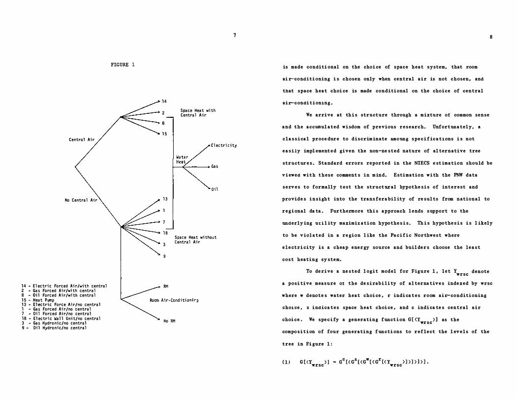
Fi gure 1 illustrate s the ne sted logit cho i ce model of four
spa ce heating sy stems with central air-conditi oning, six spa ce heating
systems without central air, water heat fuel choice , and room air
condi t1oning . The postulated structure assumes that water heat cho i ce
Central Air
No Central Air
14 - Electric Forced Air/with central 2 - Gas Forced Air/with central B - Oil Forced Air/with central 15 - Heat Pump 13 - Electric Force Air/no central l - Gas Forced Air/no central 7 - Oil Forced Air/no central l B - Electric Wa 11 Unit/no central 3 - Gas Hydronic/no central 9 - Oil Hydroni c/no central
FIGURE 1
7
14
2 Space Heat with Central Air
--, e
15 I
Electricity
Gas
Oil
I 13
l
7
18 Space Heat without
3 Central Air
RM
No RM
8
is made conditi onal on the choi ce of spac.e heat system, that room
ai r-conditi oning i s chosen only when central air is not chosen, and
that space heat choi ce is made conditional on the choice of central
air-condi tioning .
We arrive at thi s structure through a mixture of common sense
and the accumul ated wisdom of previous research. Unfortunately, a
c l a s s i cal proce dure to discrim inate amoung spe c i f ications i s not
e a s i ly impl ement e d given the non-ne sted nature of al ternative tree
structur e s . Standard errors reported in the NIECS e st imation should be
v i ewed with these comment s in m ind. Estimation with the PNW data
serv e s to formally test the structural hypothe sis of interest and
provide s insight into the trans ferabil ity of re sul ts from national to
r e g i onal da ta . Furthermore thi s approach l ends support to the
underly ing uti l ity maximiz ation hypothe s i s . Th i s hypothe s i s i s l ikely
to be v iol ated in a re gion l ike the Pac i f i c Northwest where
e l e ctri city is a cheap energy source and buil de r s choose the least
cost heating sy stem.
To de rive a ne sted l ogit model for Figure 1 , l e t Ywrsc denote
a posi tive measure ot the de sirab i l i ty of al terna tive s indexed by wrsc
where w denote s water heat choi ce , r indi ca tes room air-conditioning
choi ce , s indica tes space heat choi ce , and c indi ca te s central air
choi ce . We spe c i fy a generating funct i on G[<Ywrsc
)] as the
compo sition of four generating functi ons to reflect the l ev e l s of the
tree in Fi gure 1 :
( 1 ) G [ <Ywrsc
>) Gc
[<Gs
[<Gw
[<Gr
[<Y >1>1>1>]. wrsc
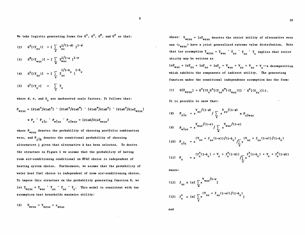
We take logistic generating forms for Ge, Gs. Gw, and Gr so that:
C2)
C3J
c 4)
CS)
Gr[<Y >l re = r [ y1/c1-d> 11-d re r
G"'[<Y >l = [ L yl/1-a 11-a WSC WSC w
1/1-"6 1-5 Gs [ <Y > 1 =C[Y cl c
SC SC s
Ge [ <Y > 1 = [ye c c
where d, a, and 5c are unobserved scale factors. It follows that:
9
P = [alnGc/alnGs1 • [alnGs/alnG"'l • [alnGw/alnGr1 • [CllnGr/alnY ] wrsc wrsc
P • P I · P I · P I = CCllnG/CllnY 1 c s c w sc r wsc wrsc
where Pwrsc denotes the probability of choosing portfolio combination
wrsc, and Pjlk denotes the conditional probability of choosing
alternative j given that alternative k has been selected. To derive
the structure in Figure 1 we assume that the probability of having
room air-conditioning conditional on HVAC choice is independent of
heating system choice. Furthermore, we assume that the probability of
water heat fnel choice is independent of room air-conditioning choice.
To impose this structure on the probability generating function G, we
let Y = Y • Y wrsc wsc re Y • Y . This model is consistent with the SC C
assumption that households maximize ntility:
c 6) u wrsc v + & wrsc wrsc
10
where: Vwrsc = lnYwrsc denotes the strict utility of alternative wrsc
and (&wrsc> have a joint generalized extreme value distribution. Note
that tne assumption Ywrsc utility may be written as
y wsc y re Ysc • Ye implies that strict
lnYwsc + lnYrc + lnYsc + lnYc = Vwsc + Vrc + Vsc + Vc�a decomposition
which exhibits the components of indirect utility. The generating
function under the conditional independence assumption has the form:
C7) G[Y 1 wrsc Gc[<Y Gs[<Y Gw[<Y >11 C SC WSC Gr[<Y >1>J. re
It is possible to show that:
c 8)
C9)
ClO)
prlc v /Cl-d) V /Cl-d) re / L re = e e =
P I r wsc r
V /Cl-a) V /Cl-a) p - wsc I L wsc
I - e e W SC w
p sic CV SC + J Cl-a))/Cl-5 ) CV + J Cl-al)/Cl-5 ) sc c /[ e sc sc c = e
s
CJsCl-5 ) + V + JrCl-5)) JsCl-5 ) + V + JrCl-d)) Cll) p c = e c c c c /[e c c c c
where:
Cl2)
Cl3)
and
J = ln[ L V wsc/1-a
SC e 1
w
c
JS = ln[ Le
CV sc + 1scCl-all/Cl-5 ) c 1 c s
( 14) Jr c � ln[ L evrJ<l-rJ)
r 1
The terms Js, Jr, and J are, respectively, the inclusive C C SC
11
values of space heat choice given central air choice, room air choice
given central air choice, and water heat choice given space heat and
central air choice; the symbols ( 1-d) , (l-6c)' and ( 1-a) are the
corresponding inclusive value coetficients.3 Here we allow the
inclusive value coefficient (l-6c) to be different depending on
central air choice to reflect a possible dissimilarity in the degree
of association in the space heat choice branches. Estimation ot the
central air conditioning choice model will identify the coefficients
6c.
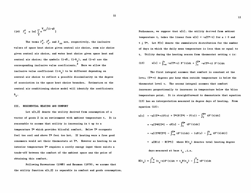
III. RESIDENTIAL HEATING AND COMFORT
Let u[t,Z] denote the utility derived from consumption of a
vector of goods Z in an environment with ambient temperature t. It is
reasonable to assume that utility is increasing in t up to a
temperature T• which provides blissful comfort. Below T* occupants
feel too cool and above T• feel too hot. If heating were a free good
consumers would set their thermostats at T*. However as heating to an
interior temperature T* requires a costly energy input there exists a
trade-off between the comfort of the ambient space and the price of
obtaining this comfort.
Following Brownstone ( 1 9 80) and Hausman ( 1979) , we assume that
the utility function u[t,Z] is separable in comfort and goods consumption.
Futhermore, we suppose that u[t], the utility derived from ambient
temperature t, takes the linear form u[t] = -a[T*-t] for a > 0 and
t � T*. Let F[t] denote the cummulat1ve distribution for the number
of days in which the daily mean temperature is less than or equal to
t. Utility during the heating season from thermostat setting T is:
( 1 5 ) u[T] = ('t' -a(T*-c) F'(t)dt + fT* -a(T*-t) F'(t)dt J-m J�
The first integral assumes that comfort is constant at the
leveJ. (T*-c) degrees per hour when outside temperature is below the
thermostat level T. The second integral assumes that comfort
increases proportionally to increases in temperature below the bliss
12
temperature point. It is straightforward to demonstrate that equation
( 1 5 ) has an interpretation measured in degree days of heating. From
equation ( 15 ) :
u[T] = -a[(T*-c)F(T) + T*(F(T*) - F(T)) - I!* tF'(t)dt]
H[t0]
= -a[T•F[T•] - TF[T] - J!* tF'(t)dt]
= -a[(T*F[T*] - s:: tF'(t)dt) - (TF(T) - t� tF'(t)dt)]
a[H(T) - H(T*)] where H(t0) denotes total heating degree
days measured at base t0 , i.e.
t f_� (t -t)F' (t)dt 0
t t F(t ) - f o tF'(t)dt 0 0 -Cl)
13
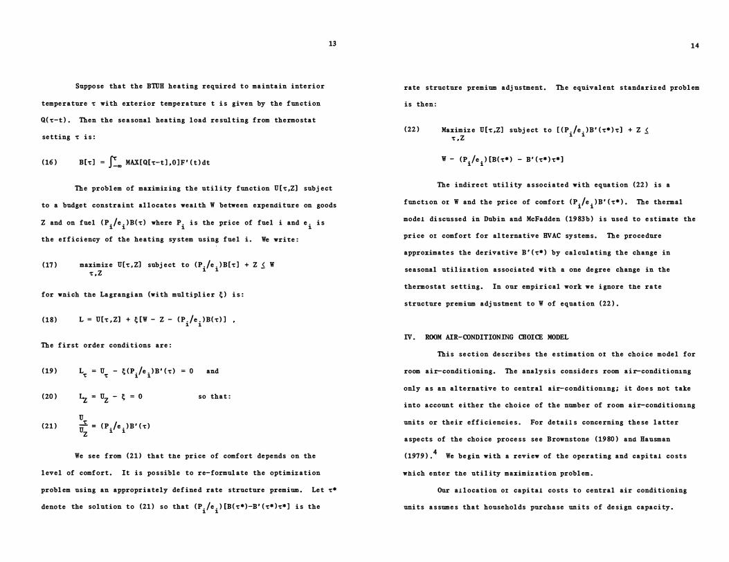
Suppose that the B'IUH heating required to maintain interior
temperature • with exterior temperature t is given by the function
Q(•-t). Then the seasonal heating load resulting from thermostat
setting • is:
(16) B[•] = .r::.= MAX[Q[•-t],O]F'(t)dt
The problem of maximizing the utility function U[•,Z] subject
to a budget constraint allocates wealth W between expenaiture on goods
Z and on fuel (P./e.)B(•) where P. is the price of fuel i and e. is i i i i the efficiency of the heating system using fuel i. We write:
(17) maximize U[•,Zl subject to (P./e.)B[•] + Z < W i i -•• z
for wnich the Lagrangian (with multiplier �) is:
(18) L = U[•,Z] + �[W - Z - (P./e.)B(•)] i i
The first order conditions are:
(19)
(20)
(21)
L = U -�(P./e.)B'(•) = 0 • • i i
Lz = Uz-�=O
u --!. = (P./e.)B'(•) uz i i
and
so that:
We see from (21) that the price of comfort depends on the
level of comfort. It is possible to re-formulate the optimization
problem using an appropriately defined rate structure premium. Let •*
denote the solution to (21) so that (P./e.)[B(•*)-B'(•*l•*] is the i i
14
rate structure premium adjustment. The equivalent standarized problem
is then:
(22) Maximize U[•,Z] subject to [(P./e.)B'(•*)•] + Z < i i -•• z
W - (P./e.)[B(•*) - B'(•*)•*] i i
The indirect utility associated with equation (22) is a
function or W and the price of comfort (P./e.)B'(•*). The thermal i i model discussed in Dubin and McFadden (1983b) is used to estimate the
price or comfort for alternative HVAC systems. The procedure
approximates the derivative B'(•*) by calculating the change in
seasonal utilization associated with a one degree change in the
thermostat setting. In our empirical work we ignore the rate
structure premium adjustment to W of equation (22).
IV. ROOM AIR-CONDITIONING CHOICE MODEL
This section describes the estimation or the choice model for
room air-conditioning. The analysis considers room air-conditioning
only as an alternative to central air-conditioning; it does not take
into account either the choice of the number of room air-conaitioning
units or their efficiencies. For details concerning these latter
aspects of the choice process see Brownstone (1980) ana Hausman
(1979).4 We begin with a review of the operating and capital costs
which enter the utility maximization problem.
Our allocation or capital costs to central air conditioning
units assumes that households purchase units of design capacity.
15
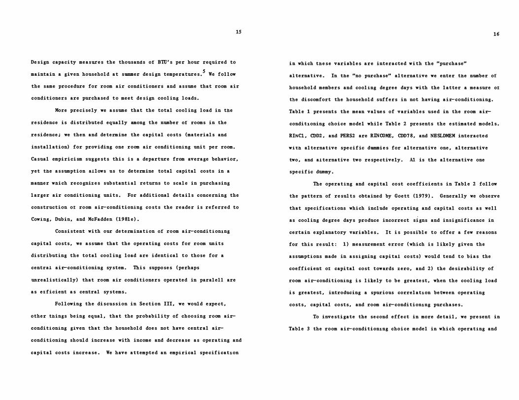
Design capacity measures the thousands of B'IU's per hour required to
maintain a given household at summer design temperatures. 5 We follow
the same procedure for room air conditioners and assume that room air
conditioners are purchased to meet design cooling loads.
More precisely we assume that the total cooling load in the
residence is distributed equally among the number of rooms in the
residence; we then and determine the capital costs (materials and
installation) for providing one room air conditioning unit per room.
Casual empiricism suggests this is a departure from average behavior,
yet the assumption allows us to determine total capital costs in a
manner wnich recognizes substantial returns to scale in purchasing
larger air conditioning units. For additional details concerning the
construction ot room air-conditioning costs the reader is referred to
Cowing, Dubin, and McFadden (1981e).
Consistent with our determination of room air-conditioning
capital costs, we assume that the operating costs for room units
distributing the total cooling load are identical to those for a
central air-conditioning system. This supposes (perhaps
unrealistically) that room air conditioners operated in paralell are
as exficient as central systems.
Following the discussion in Section III, we would expect,
other things being equal, that the probability of choosing room air
conditioning given that the household does not have central air-
conditioning should increase with income and decrease as operating and
capital costs increase. We have attempted an empirical specification
16
in which these variables are interacted with the "purchase"
alternative. In the "no purchase" alternative we enter the number of
household members and cooling degree days with the latter a measure ot
the discomfort the household suffers in not having air-conditioning.
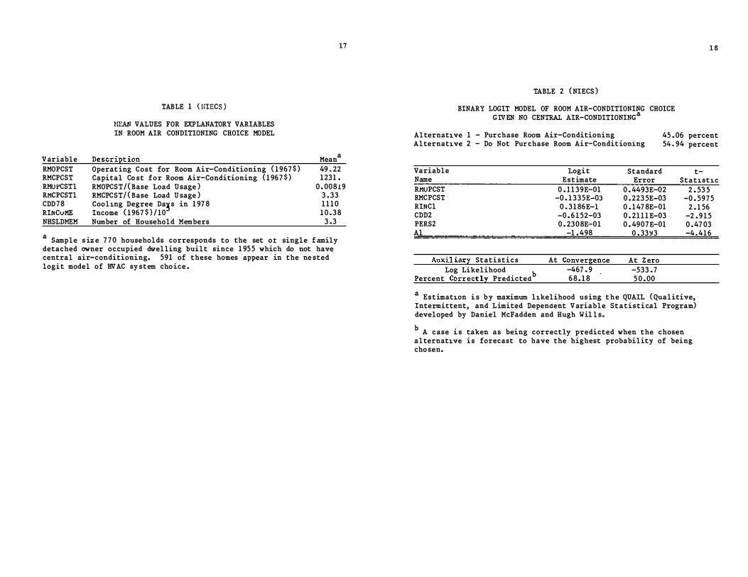
Table 1 presents the mean values of variables used in the room air-
conditioning choice model while Table 2 presents the estimated models.
RINCl, CDD2, and PERS2 are RINCOME, CDD78, and NHSLDMEM interacted
with alternative specific dummies for alternative one, alternative
two, and alternative two respectively. Al is the alternative one
specific dummy.
The operating and capital cost coefficients in Table 2 follow
the pattern of results obtained by Goett (1979). Generally we observe
that specifications which include operating and capital costs as well
as cooling degree days produce incorrect signs and insignificance in
certain explanatory variables. It is possible to offer a few reasons
for this result: 1) measurement error (which is likely given the
assumptions made in assigning capital costs) would tend to bias the
coefficient ot capital cost towards zero, and 2) the desirability of
room air-conditioning is likely to be greatest, when the cooling load
is greatest, introducing a spurious correlation between operating
costs, capital costs, and room air-conditioning purchases.
To investigate the second effect in more detail, we present in
Table 3 the room air-conditioning choice model in which operating and
V ariable RMOPCST RMCPCST RMUl'CSTl RMCPCSTl CDD78 RI.NCuME NHSLDMEM
TABLE 1 (UIECS)
MEAN VALUES FOR EXPLANATORY VARIABLES IN ROOM AIR CONDITIONING CHOICE MODEL
De s cript ion Operat ing Cost for Room Air-Conditioning ( 1 967$) Capital Co st for Room Air-Conditioning ( 1 967$) RMOPCST/( Base Load U sage ) RMCPCST/ ( Base Load U sage ) Cooling Degree Da!s in 1 97 8 Income ( 1 967 $ ) / 10 Number of Household Members
17
a Mean 49 . 22 1231 .
0 . 00819 3 . 33 1 1 1 0 1 0 . 3 8
3 .3
a Sample s iz e 7 7 0 households corresponds to the set ot single family detached owner occupied dwelling built since 1 95 5 which do not have central air-conditioning. 591 of these homes appear in the ne sted logit model of HVAC sy stem cho ice .
TABLE 2 ( NIECS )
BINARY LOGIT MODEL OF ROOM AIR-CONDITIONING CHOICE GIVEN NO CENTRAL AIR-CONDITIONINGa
18
Alternative 1 - Purchase Room Air-Conditioning Alternative 2 - Do Not Purchase Room Air-Conditioning
45 . 06 percent 54 . 94 percent
Variable Lo git Name Estimate RMUPCST 0 . 1 1 3 9E-01 RMCPCST -0 . 1 335E-03 RINCl 0 . 3 1 86E-l CDD2 -0 . 6 1 52-03 PERS2 0 . 23 0 8E-01 Al -1 . 498
Auxiliary Statistics At Convergence Log Likelihood b
-467 . 9 Percent Correctly Predicted 6 8 . 1 8
Standard Error
0 . 4493E-02 0 . 223 5E-03 0 . 147 8E-01 0 . 21 1 1 E-03 0 . 4907E-01
0 . 33Y3
At Z ero -533 .7 5 0 . 00
t-Statistic
2 . 53 5 -0 . 5975
2 . 1 56 -2 . 9 1 5 0 . 47 03 -4.416
a Estimation i s by maximum likelihood us ing the QUAIL ( Qualitive, Intermittent, and Limited Dependent V ariable Statistical Program) developed by Daniel McFadden and Hugh Wills.
b A case i s taken as being correctly predicted when the chosen alternative is forecast to have the highest probability of being cho sen.
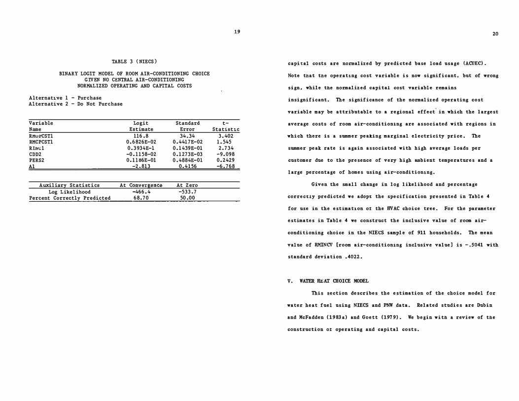
TABLE 3 (NIE CS )
BINARY LOGIT MODEL OF ROOM AIR-CONDITIONING CHOICE GIVEN NO CENTRAL AIR-CONDITIONING
NORMALIZED OPERATING AND CAPITAL COSTS
Alternative 1 - Purchase Alternative 2 - Do Not Purchase
Variable Name RMu!'CSTl RMCPCSTl R!J.11�1 CDD2 PERS2 Al
Lo git Estimate
116 . 8 0 . 6 826E-02 0 . 3 934E-l
-0 . 1 1 58-02 0 . 1 1 86E-01
-2 . 813
Auxil iary Stati st i cs At Conver�ence Log L ikelihood -466 . 4
Percent Correctly Predicted 6 8 . 7 0
Standard Error 34.34
0 .441 7E-02 0 . 1439E-01 0 . 1 273E-03 0 .4884E-01
0 .4 1 56
At Z ero -533 . 7 50 .00
19
t-Statistic
3 . 402 1 . 545 2 . 7 34
- 9 . 098 0 . 2429 -6 . 7 6 8
20
capi�al costs are normalized by predicted base load usage (ACUEC) .
Note that the operating cost variable is now significant, but of wrong
sign, while the normalized capital cost variable remains
insignificant. The significance of the normalized operating cost
variable may be attributable to a regional effect in which the largest
average costs of room air-conditioning are associated with regions in
which there is a summer peaking marginal electricity price. The
summer peak rate is again associated with high average loads per
customer due to the presence of very high ambient temperatures and a
large percentage of homes using air-conditioning.
Given the small change in log likelihood and percentage
correc�ly predicted we adop� the specification presented in Table 4
for use in the estimation ot the HVAC choice tree. For the parameter
estimates in Table 4 we construct the inclusive value of room air-
conditioning choice in the NIECS sample of 911 households. The mean
value of RMINCV [room air-conditioning inclusive value] is -.5041 with
standard deviation . 4022.
V. WATER H.t: AT CHOICE MODEL
This section describes the estimation of the choice model for
water heat fuel using NIECS and PNW data. Related studies are Dubin
and McFadden (1983a) and Goett (1979). We begin with a review of the
construction ot operating and capital costs.
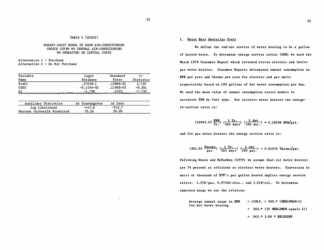
TABLE 4 ( NIECS )
BINARY LOGIT MODEL OF ROOM AIR-CONDITIONING CHOICE GIVEN NO CENTRAL AIR-CONDITIONING
NO OPERATING OR CAPITAL COSTS
Alternative 1 - Purchase Alternative 2 - Do Not Purchase
Variable Name RINCl CDD2 Al
Logit Estimate . 3 7 6 5E-l
-0 . 1 1 04-02 -1 . 7 96
Auxiliary Statistics At Convergence Log Likelihood -4/2 . 6
Percent Correctly Predict ed 70 . 26
Standard Error
. 1380E-01
. 1 1 90E-03 . 23 22
At Z ero -533 . 7 50 . 00
21
t-Statistic
2. 7 29 -9 . 281 -7 . 732
1. Water Heat Operating Costs
22
We define the end-use service of water heating to be a gallon
of heated water. To determine energy service ratios (ESR) we used the
March 1978 Consumer Report which reviewed eleven electric and twelve
gas water heaters. Consumer Reports determined annual consumption in
KWH per year and therms per year for electric and gas units
respectively based on 100 gallons of hot water consumption per day.
We used the mean value of annual consumption across models to
calculate ESR by fuel type. For electric water heaters the energy-
to-service ratio is:
KWH 1 Yr. ) ( 1 day ) (10434. 5 5 Yr.> C365 days 100 dal. 0 .285 88 KWH/ gal.
and for gas water heaters the energy service ratio is:
(502•33 Therms) ( 1 Yr. ) ( 1 day ) gas 365 days 100 gal. 0.01376 Therms/gal.
Following Duoin and McFadden (1979) we assume that oil water heaters
are 74 percent as efficient as electric water heaters. Conversion to
uni�s of thousand of B1U's per gallon heated implies energy service
ratios: 1. 376-gas, 0.97542-elec., and 1.318-oil. To determine
expec�ed usage we use the relation:
Average annual usage in KWH = (2819. + 360.* (NHSLDMHM-2) for hot water heating
+ 360.* (If NHSLDMEM equals 1))
+ 365.* 3.98 * HELDISHW
23
This equation is discussed in Dubin and McFadden (1983a).
Note tnat NHSLDMEM and HELDISHW are, respectively, the number of
household members and a dummy variable indicating that the household
has a dishwasher. Finally, operating costs by fuel type are the
product of (1) expected annual usage, (2) the ratio of the ESR of the
fuel under consideration to tne ESR of the electric water heater, and
(3) the price of the fuel at the point of house construction converted
to real 1967 dollars.
2. Water Heat Capital Costs
Construction ot water heating capital costs requires a
relationship between assumed capacity and structural characteristics
of the dwelling and family. We follow the recommended practice
(nHandbook of Buying 1978," Consumer Research Magazine) of relating
capacity utilization to the number of bathrooms and the number of
bedrooms (a proxy for number of persons). This relationship includes
allowance for recovery rate differentials that occur between fuel
types. Materials and installation costs for different capacity water
heaters are obtained from MEANS (1981). These estimates 4o not
include the vent costs for each water heater. We consulted the
National Construction Estimator (Craftsman Book Co. , Solano Beach, CA
1978) and determined that in 1981 dollars material costs would be $18 while installation costs would be $26. The National Construction
Estimator also indicated electrical contracting charges of $145 and
$161 for water heaters with capacity less than and greater than 40
gallons. These costs were included in the installation costs obtained
24
from MEANS (1981). Finally, we have included all cost components which
are conditional on the type of space heating system installed. When
space heating type is gas or electric, the cost for materials and
installation of an oil tank are included with the costs of oil water
heating. When space heating type is gas or oil, an additional charge
of $112 is added to the labor costs of the electric water heater due
to tne installation ot increased amp service (National Construction
Estimator, 1978). Other charges for all systems are assumed reflected
in tne cost of the heating systems.
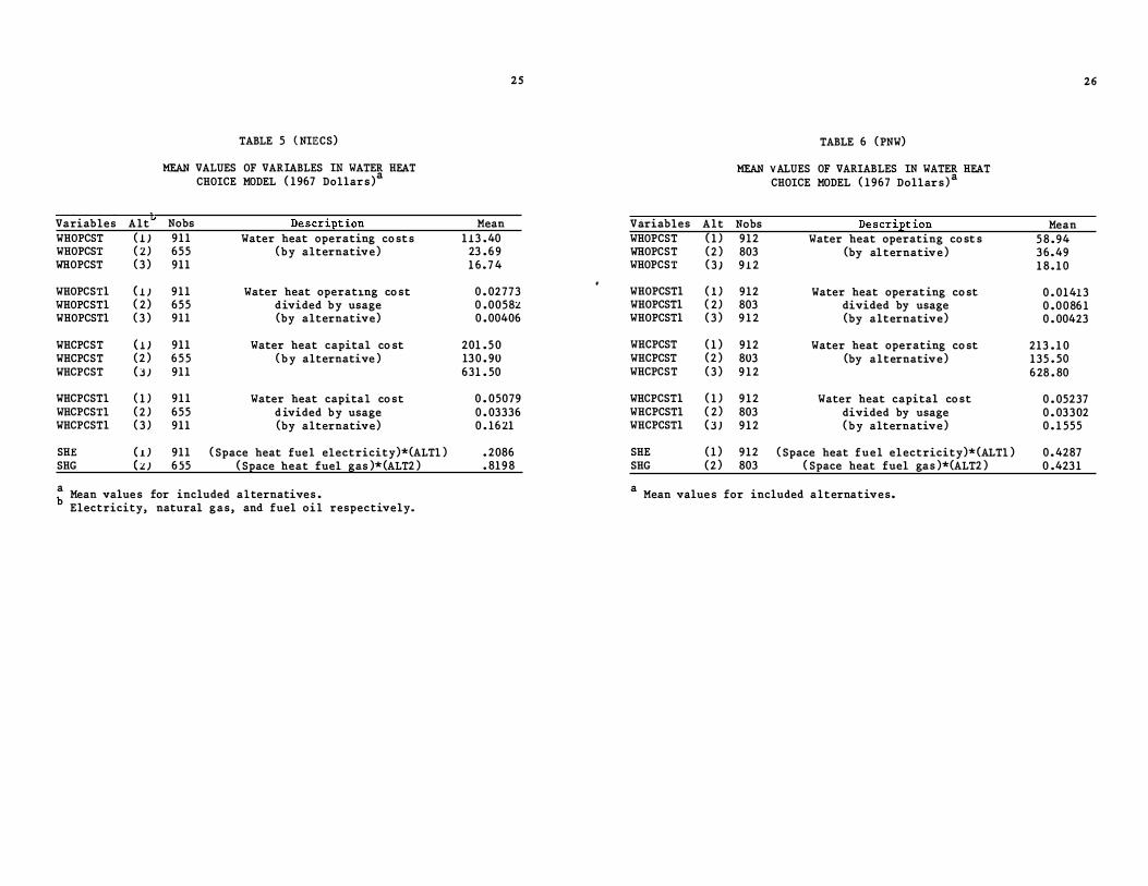
3. Estimation of Water Heat Choice Model
Tables 5 and 6 present the mean values of NIECS and PNW
variables used in the choice models as well as their descriptions.
Estimation is based on a sample of households who live in single
family owner occupied dwellings built since 1955 and who choose either
electric, gas, or oil water heaters. 6 As discussed above, the natural
gas alternative is eliminated from the choice set whenever gas is
unavailable to the household. Thus, in Table 5, the number of
includea ooservations drops from 911 in the electric and oil
alternatives to 655 in the natural gas alternative. A similar effect
is seen in Table 6.
We considered both binary and trinary specifications which
used water heat operating and capital costs as well as space heat
fuel-type dummies as explanatory variables. Models in which costs
were not aajusted for scale provided generally wrong signs on
variables and were difficult to interpret.
25 26
TABLE 5 (NIE CS) TABLE 6 (PNW)
MEAN VALUES OF VARIABLES IN WATER HEAT MEAN VALUES OF VARIABLES IN WATER HEAT CHOICE MODEL ( 1 967 Dollar s )a
CHOICE MODEL ( 1 967 Dollar s ) a
Variables Alt Nobs DescriEt ion Mean V ariables Alt Nobs De scriEtion Mean WHOPCST ( ! ) 911 Water heat operating co st s 1 !3 . 40 WHOPCST ( 1 ) 912 Water heat operating co st s 5 8 . 94 WHOPCST ( 2 ) 655 (by alternative) 23 . 6 9 WHOPCST ( 2 ) 803 (by al ternativ e ) 3 6 . 49 WHOPCST ( 3 ) 911 1 6 . 7 4 WHOPCST ( 3 ) 9 1 2 1 8 . 1 0
. WHOPCSTl (lJ 911 Water heat operating co st 0 . 02773 WHOPCSTl (1) 912 Water heat operating co st 0 . 01413 WHOPCSTl ( 2) 655 divided by usage 0 . 0058:.! WHOPCSTl ( 2) 803 divided by usage 0 . 0086 1 WHOPCSTl ( 3 ) 911 (by alternative) 0 . 00406 WHOPCSTl ( 3 ) 9 1 2 (by alternative) 0 . 00423
WHCPCST (lJ 911 Water heat capital co st 201 . 5 0 WHCPCST ( 1 ) 912 Water heat operating co st 213 . 1 0 WHCPCST ( 2 ) 6 5 5 ( b y alternative ) 13 0 . 90 WHCPCST ( 2 ) 803 (by alternative) 135 .so WHCPCST (jJ 911 631 . 50 WHCPCST ( 3 ) 9 1 2 6 28 . 80
WHCPCSTl ( 1 ) 911 Water heat capital co st 0 . 05079 WHCPCSTl ( 1 ) 9 1 2 Water heat capital co st 0 . 05237 WHCPCSTl ( 2 ) 655 d ivided by usage 0 . 03336 WHCPCSTl ( 2) 803 divided by usage 0 . 03302 WHCPCSTl ( 3 ) 911 (by alternative) 0 . 1621 WHCPCSTl (3) 9 1 2 ( b y alternative) 0 . 1 555
SHE (1) 911 ( Space heat fuel electricity)*(ALTl ) . 2086 SHE ( 1 ) 912 ( Space heat fuel el ectricity)*(ALTl ) 0 . 4287 SHG (:.!) 655 ( Space heat fuel gas )*(ALT2 ) . 81 9 8 SHG ( 2 ) 803 ( Space heat fuel gas )*(ALT2 ) 0 .423 1
� Mean value s for included alternatives . a Mean value s for included alternatives. Electricity, natural gas, and fuel oil respectively.
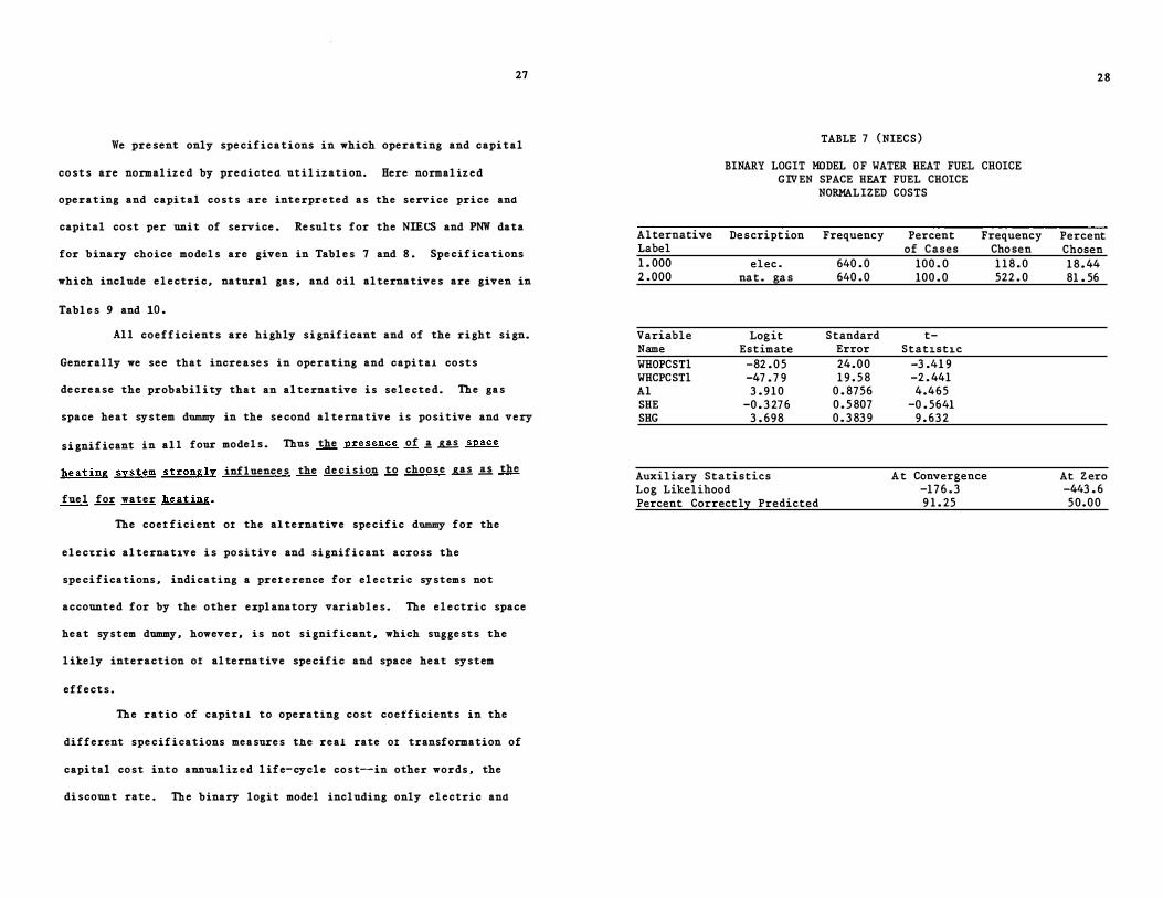
27
We present only specifications in which operating and capital
costs are normalized by predicted ntilization. Here normalized
operating and capital costs are interpreted as the service price and
capital cost per unit of service. Results for the NIECS and PNW data
for binary choice models are given in Tables 7 and 8 . Specifications
which include electric, natural gas, and oil alternatives are given in
Tables 9 and 10 .
All coefficients are highly significant and of the right sign.
Generally we see that increases in operating and capita! costs
decrease the probability that an alternative is selected. The gas
space heat system dummy in the second alternative is positive and very
significant in all four models. Thus the presence of � � space
heating system strongly influences the decision to choose � .!£ the
fuel for water heating.
The coetficient or the alternative specific dummy for the
elec�ric alternative is positive and significant across the
specifications, indicating a preterence for electric systems not
accounted for by the other explanatory variables. The electric space
heat system dummy, however, is not significant, which suggests the
likely interaction ot alternative specific and space heat system
effects.
The ratio of capital to operating cost coetficients in the
different specifications measures the real rate or transformation of
capital cost into annualized life-cycle cost--in other words, the
discount rate. The binary logit model including only electric and
TABLE 7 ( NIECS)
BINARY LOGIT MODEL OF WATER HEAT FUEL CHOICE GIVEN SPACE HEAT FUEL CHOICE
Alternative De script ion Label 1 . 000 elec . 2 . 000 nat . ga s
Variable Log it Name Estimate WHOPCSTl -82 . 0 5 WHCPCSTl -47 . 7 9 Al 3 . 9 1 0 SHE -0 . 3 276 SHG 3 . 698
Auxiliary Statistics Log Likelihood Percent Correctly Predicted
NORMALIZED COSTS
Frequency
640 . 0 640 . 0
Standard Error 24. 0 0 1 9 . 5 8
0 . 8756 0 . 5 807 0 . 3 83 9
Percent Frequency of Cases
100 . 0 100 . 0
t-Statistic
-3 .41 9 -2 . 441 4.465
-0 . 5641 9 . 63 2
A t Convergence -1 7 6 . 3 9 1 . 25
Cho sen 1 1 8 . 0 522 . 0
28
Percent Chosen 1 8 . 44 81 . 56
At Z ero -443 . 6 5 0 . 0 0
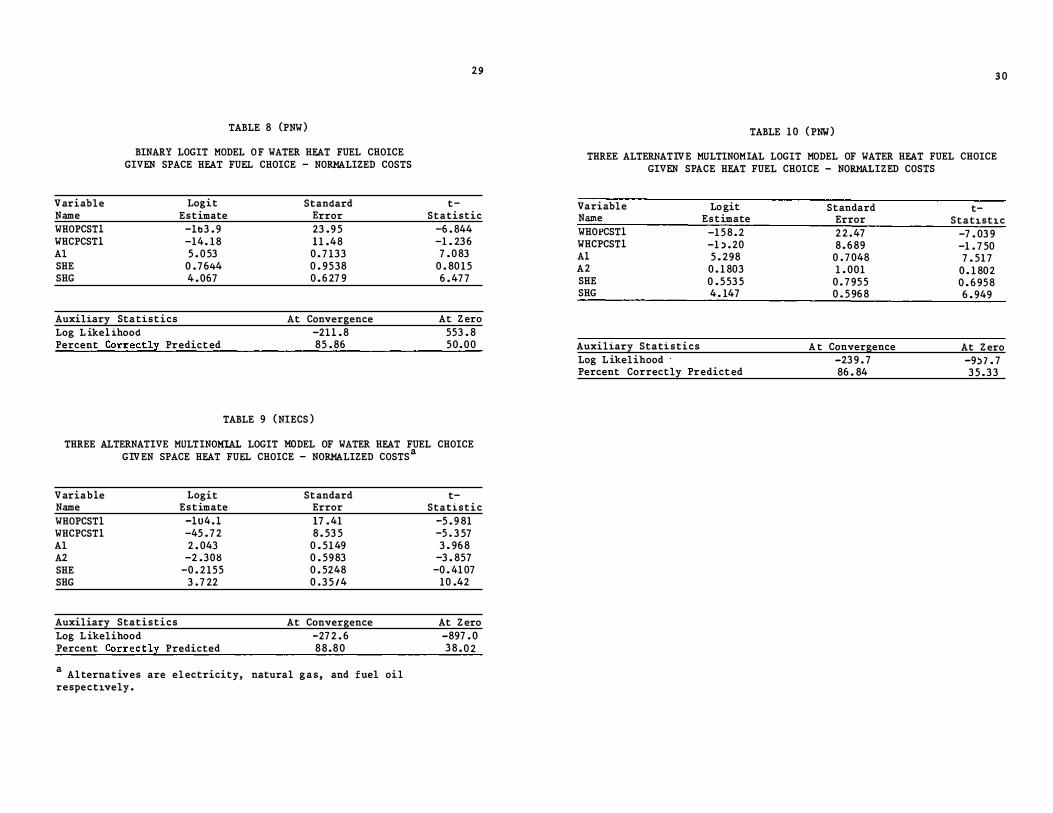
TABLE 8 (PNW)
BINARY LOGIT MODEL OF WATER HEAT FUEL CHOICE GIVEN SPACE HEAT FUEL CHOICE - NORMALIZED COSTS
V ariable Lo git Standard Name Estimate Error WHOPCSTl -lb3 . 9 23 . 9 5 WHCPCSTl -14. 1 8 1 1 .48 Al 5 . 0 53 0 . 7 133 SHE 0 . 7644 0 . 9538 SHG 4 . 067 0 . 6 27 9
Auxiliary Statist ics At Convergence Log L ikel ihood -2ll . 8 Percent Correctly Predict ed 85 . 86
TABLE 9 ( NIECS )
29
t-Statistic
-6 . 844 -1 . 23 6 7 . 0 83
0 . 80 1 5 6 . 47 7
At Z ero 553 . 8 5 0 . 0 0
THREE ALTERNATIVE MULTINOMIAL LOGIT MODEL OF WATER HEAT FUEL CHOICE GIVEN SPACE HEAT FUEL CHOICE - NORMALIZED COSTSa
V ariable Lo git Standard Name Estimate Error WHOPCSTl -lu4.l 17 . 41 WHCPCSTl -45 . 7 2 8 . 53 5 Al 2 . 043 0 . 51 49 A2 -2 .308 0 . 5983 SHE -0 . 2155 0 . 5248 SHG 3 . 7 22 0 . 3 5/4
Auxiliary Statistics At Convergence Log L ikelihood -27 2 . 6 Percent Correctly Predicted 8 8 . 8 0
a Alternatives are electricity, natural g a s , and fuel oil respectively .
t-Statistic
-5 . 9 81 -5 . 3 57 3 . 96 8
-3 . 857 -0 . 41 07
10 .42
At Z ero -897 . 0 3 8 . 0 2
3 0
TABLE 1 0 ( PNW)
THREE ALTERNATIVE MULTINOMIAL LOGIT MODEL OF WATER HEAT FUEL CHOICE GIVEN SPACE HEAT FUEL CHOICE - NORMALIZED COSTS
Variable Lo git Name Estimate WHOPCSTl -1 5 8 . 2 WHCPCSTl -1 ' . 20 Al 5 . 298 A2 0 . 1 803 SHE 0 . 5 53 5 SHG 4 . 147
Auxiliary Stati stics Log L ikelihood Percent Correctly Predict ed
Standard Error 2 2 . 47 8 . 6 89
0 . 7 048 1 . 001
0 . 7 95 5 0 . 5 96 8
A t Convergence -23 9 . 7 86 . 84
t-Statistic
-7 . 03 9 -1 . 7 50 7 . 51 7
0 . 1 802 0 . 6 95 8 6 . 949
At Z ero -9'.:>7 . 7 3 5 . 3 3
31
natural gas alternatives implies that these discount factors are 58.24
percent and 8.65 percent for the NIECS and PNW data respectively. The
trinary muae1s imply discount factors of 43.92 percent and 9.61
percent for the NIECS and PNW data respectively.
These differences in estimated discount rates are too large to
be explained away through minor changes in the modeling assumptions.
One likely explanation is that the historically low price of
electricity in the Pacific Northwest lead to a high saturation of
elec�ric water heat systems with much smaller attention paid to
ini�ial capital costs. This effect is further seen in the
coefficients of capital costs in Tables 8 and 10 . Although the
qualitative results are very similar, it would not appear that the
national results are directly transferable to a region such as the
Pacific Northwest, where energy prices have had such a profoundly
different history.
We use the choice model in Table 9 in the estimation of the
HVAC nested logit model. The calculation ot inclusive values correctly
accounts for the availability of natural gas. Thus, when gas is not
available, the inclusive value corresponds to the electric and oil
alternatives only.
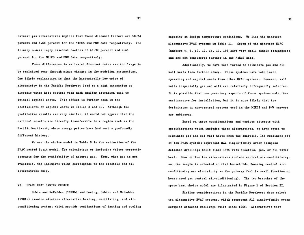
VI. SPACE HEAT SYSTEM CHOICE
Dubin and McFadden (1983b) and Cowing, Dubin, and McFadden
(1�8le) examine nineteen alternative heating, ventilating, and air
conditioning systems which provide combinations of heating and cooling
32
capacity at design temperature conditions. We list the nineteen
alternative HVAC systems in Table 11 . Seven of the nineteen HVAC
(numbers 4, 6, 1 0 , 12, 16, 17 , 19) have very small sample frequencies
and are not considered further in the NIECS data.
Additionally, we have been forced to eliminate gas ana oil
wall units from further study. These systems have both lower
operating and capital costs than other HVAC systems. However, wall
units (especially gas and oil) are relatively infrequently selectea.
It is possible that non-pecuniary aspects of these systems make them
unattractive for installation, but it is more likely that the
deiinitions ot non-central systems used in the NIECS and PNW surveys
are ambiguous.
Based on these considerations and various attempts with
specifications which included these alternatives, we have opted to
eliminate gas and oil wall units from the analysis. The remaining set
of ten HVAC systems represent 911 single-family owner occupiea
detached dwellings built since 1955 with electric, gas, or oil water
heat. Four oI the ten aiternatives include central air-conditioning,
ana the sample is selected so that households choosing central air
conditioning use electricity as the primary fuel (a small fraction of
homes used gas central air-conditioning). The two branches of the
space heat choice model are illustrated in Figure 1 of Section II.
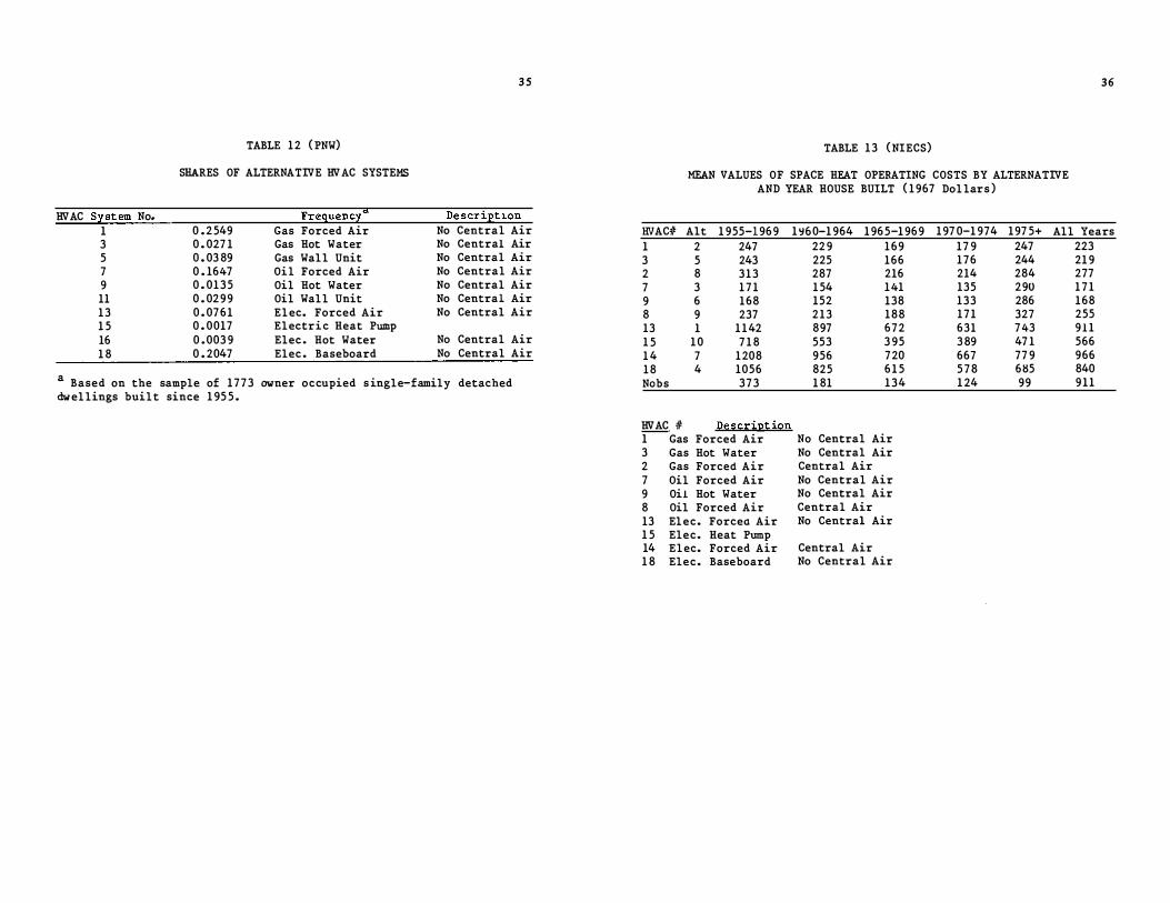
Similar considerations in the Pacific Northwest data select
ten alternative HVAC systems, which represent 912 single-family owner
occupied detached dwellings built since 1955. Alternatives that
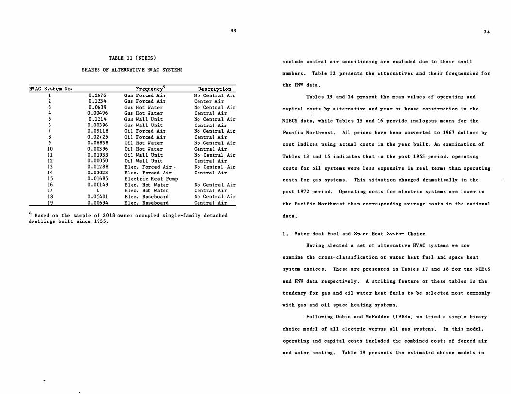
33
TABLE 1 1 ( NIECS )
SHARES OF ALTERNATIV E HVAC SYSTEMS
HVAC Szstem No. Freg,uencz a De s cri:etion 1 0 . 2676 Gas Forced Air No Central Air 2 0 . 1 23 4 Gas Forced Air Center Air 3 0 . 06 3 9 Gas Hot Water No Central Air 4 0 . 00496 Gas Hot Water Central Air 5 0 . 1214 Gas Wall Unit No Central Air 6 0 . 003 96 Gas Wall Unit Central Air 7 0 . 09 1 1 8 Oil Forced Air No Central Air 8 0 . 02/25 Oil Forced Air Central Air 9 0 . 06 83 8 Oil Hot Water No Central Air
1 0 0 . 003 96 Oil Hot Water Central Air 1 1 0 . 0 1 933 Oil Wall Unit No Central Air 12 0 . 00050 Oil Wall Unit Central Air 13 0 . 01288 Elec. Forced Air - No Central Air 14 0 . 03023 Elec. Forced Air Central Air 1 5 0 . 01 6 85 Electric Heat Pump 16 0 . 00149 Elec. Hot Water No Central Air 17 0 Elec. Hot Water Central Air 1 8 0 . 0 5401 Elec. Baseboard No Central Air 1 9 0 . 00694 Elec. Baseboard Central Air
a Based on the sample of 2018 owner o ccupied s ingle-family detached dwellings built since 1 9 5 5 .
34
include central air conaition1ng are excluded due to their small
numbers. Table 12 presents the alternatives and their frequencies for
the PNW data.
Tables 13 and 14 present the mean values of operating and
capital costs by alternative and year ot house construction in the
NIECS data, while Tables 15 and 16 provide analogous means for the
Pacific Northwest. All prices have been converted to 1967 dollars by
cost indices using actual costs in the year built. An examination of
Tables 13 and 15 indicates that in the post 1955 period, operating
costs for oil systems were less expensive in real terms than operating
costs for gas systems. This situation changed dramatically in the
post 1972 period. Operating costs for electric systems are lower in
the Pacific Northwest than corresponding average costs in the national
data.
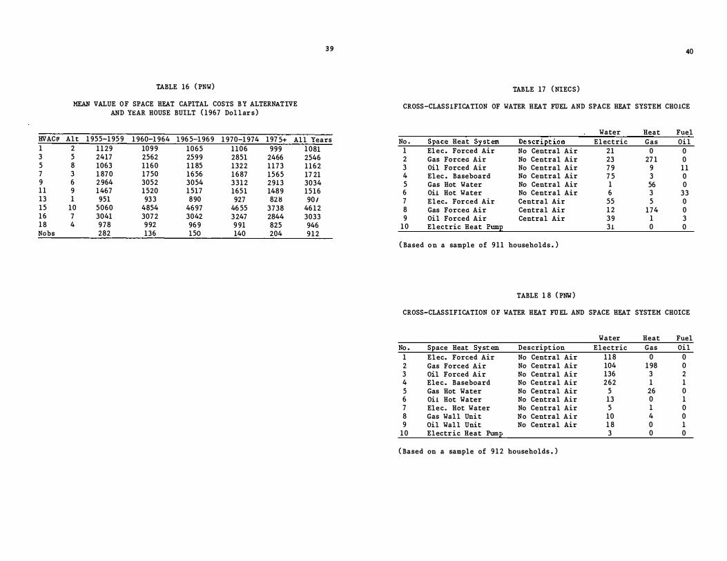
1. Water Heat Fuel and Space Heat System Choice
Having sleeted a set of alternative HVAC systems we now
examine the cross-classification ot water heat fuel and space heat
system choices. These are presented in Tables 17 and 18 for the NIE�S
and PNW data respectively. A striking feature ot these tables is the
tendency for gas and oil water heat fuels to be selected most commonly
with gas and oil space heating systems.
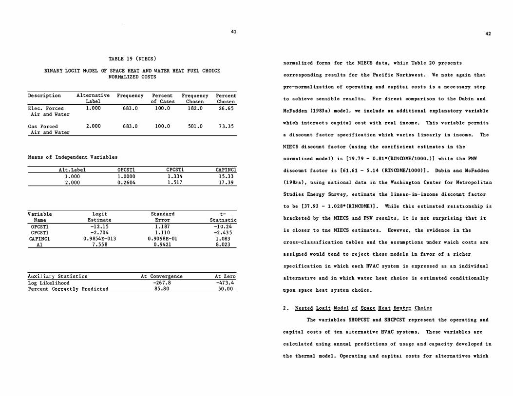
Following Dubin and McFadden (1983a) we tried a simple binary
choice model of all electric versus all gas systems. In this model,
operating and capital costs included the combined costs of forced air
and water heating. Table 19 presents the estimated choice models in
3 5
TABLE 12 ( PNW)
SHARES OF ALTERNATIVE HVAC SYSTEMS
HVAC S:z:st em No. Freg,uenc:z: a DescriEti.on 1 0 . 2549 Gas Forced Air No Central Air 3 0 . 027 1 Gas Hot Water No Central Air 5 0 . 03 89 Gas Wall Unit No Central Air 7 0 . 1647 Oil Forced Air No Central Air 9 0 . 01 3 5 Oil Hot Water No Central Air 11 0 . 0299 Oil Wall Unit No Central Air 13 0 . 07 6 1 Elec. Forced Air No Central Air 1 5 0 . 0017 Electri c Heat Pump 16 0 . 0039 Elec . Hot Water No Central Air 1 8 0 . 2047 Elec . Baseboard No Central Air
a Based on the sample of 1773 owner occupied s ingle-family detached dwellings built since 195 5 .
TABLE 13 ( NIECS)
MEAN VALUES OF SPACE HEAT OPERATING COSTS BY ALTERNATIVE AND YEAR HOUSE BUILT ( 1967 Dollars )
3 6
l:NAC# Alt 1955-1969 1!:160-1964 196 5-1969 197 0-1974 197 5+ All Years 1 2 247 3 5 243 2 8 313 7 3 1 7 1 9 6 168 8 9 237 13 1 1 1 42 1 5 1 0 7 1 8 1 4 7 1208 1 8 4 1056 Nabs 373
HVAC # Des cri2t ion 1 Gas Forced Air 3 Gas Hot Water 2 Gas Forced Air 7 Oil Forced Air 9 Oil Hot Water 8 Oil Forced Air 13 Elec. Forcea Air 1 5 Elec. Heat Pump 14 Elec. Forced Air 1 8 Elec. Baseboard
229 169 179 247 223 225 166 176 244 219 287 216 214 284 277 1 54 141 135 290 1 7 1 152 138 133 286 168 213 188 171 327 255 897 672 631 743 911 553 395 3 89 47 1 566 956 720 667 779 966 825 6 1 5 5 7 8 685 840 1 81 134 1 24 99 911
No Central Air No Central Air Central Air No Central Air No Central Air Central Air No Central Air
Central Air No Central Air
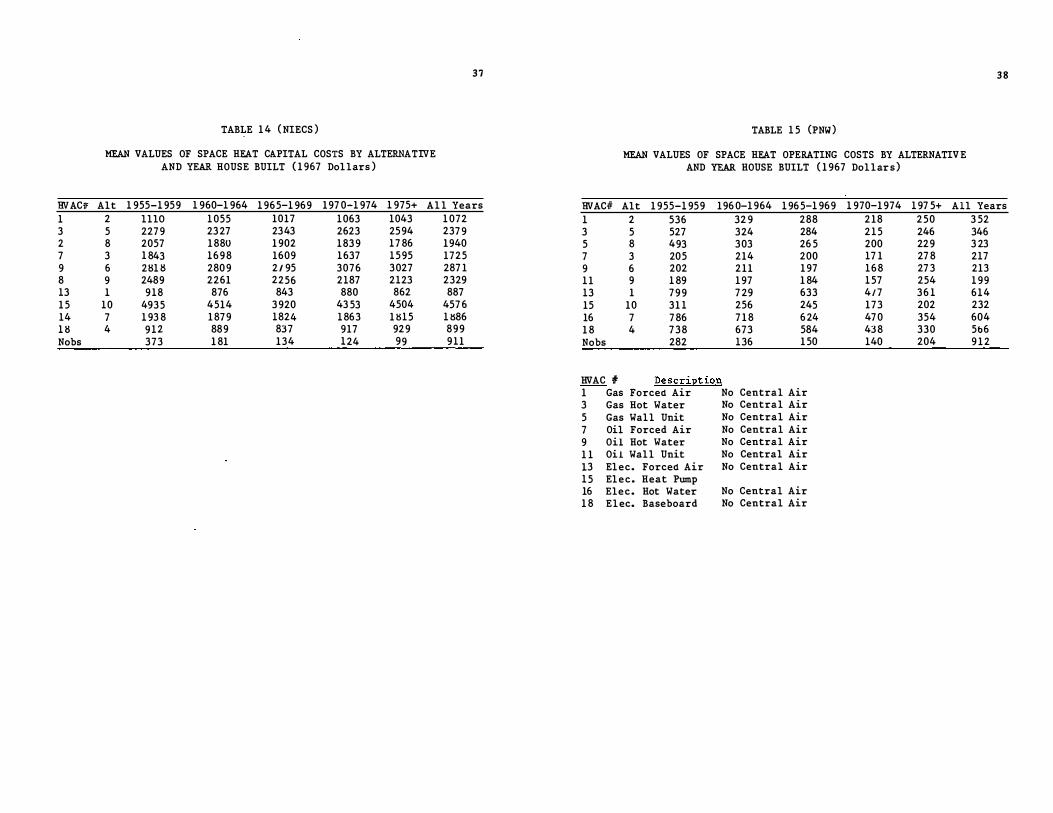
TABLE 1 4 ( NIECS )
MEAN VALUES OF SPACE HEAT CAPITAL COSTS BY ALTERNATIVE AND YEAR HOUSE BUILT (1967 Dollars )
37
RVACtF Alt 1955-1959 1960-1964 1965-1969 197 0-1974 1975+ All Years 1 2 lllO 1055 1017 1063 1043 1072 3 5 2279 23 27 2343 2623 2594 2379 2 8 2057 1 880 1902 1839 17 86 1940 7 3 1 843 169 8 1609 1637 1595 1725 9 6 2!:11!:1 2809 2/95 3076 3027 287 1 8 9 2489 2261 2256 2187 2123 2329 13 1 918 876 843 880 862 887 1 5 10 4935 4514 3920 43 53 4504 457 6 14 7 193 8 1 879 1824 1863 1!:115 1!:186 18 4 912 889 837 917 929 899 Nobs 373 1 81 134 124 99 911
TABLE 15 (PNW )
MEAN VALUES OF SPACE HEAT OPERATING COSTS BY ALTERNATIV E AND YEAR HOUSE BUILT (1967 Dollar s )
3 8
RVACifo Alt 1955-1959 196 0-1964 196 5-1969 1970-1974 197 5+ All Years 1 2 536 329 288 3 5 527 324 284 5 8 493 303 26 5 7 3 205 214 200 9 6 202 211 197 11 9 189 197 1 84 13 1 799 7 29 633 15 10 311 256 245 16 7 7 86 7 1 8 6 24 1 8 4 7 3 8 673 584 Nobs 282 136 1 50
HVAC # Description 1 Gas Forced Air 3 Gas Hot Water 5 Gas Wall Unit 7 Oil Forced Air 9 Oil Hot Water 1 1 Oil Wall Unit 13 Elec. Forced Air 15 Elec. Heat Pump 16 Elec. Hot Water 1 8 Elec. Baseboard
No Central Air No Central Air No Central Air No Central Air No Central Air No Central Air No Central Air
No Central Air No Central Air
218 250 3 52 215 246 346 200 229 3 23 17 1 27 8 217 16 8 27 3 213 157 254 199 417 361 614 173 202 232 47 0 354 604 43 8 330 5b6 140 204 9 1 2
3 9 40
TABLE 16 ( PNW) TABLE 17 ( NIE CS)
MEAN VALUE OF SPACE HEAT CAPITAL COSTS BY ALTERNATIVE CROSS-CLASSIFICATION OF WATER HEAT FUEL AND SPACE HEAT SYSTEM CHOICE AND YEAR HOUSE BUILT ( 1967 Dollar s )
Water Heat Fuel HVAC�r Alt 19SS-19S9 1960-1964 l 96 S-l 969 1970-1974 197 S+ All Years No . SEace Heat S1stem Descri:etion Electric Gas Oil 1 2 1 1 29 1099 106S 1106 999 1 081 1 Elec. Forced Air No Central Air 21 0 0 3 s 2417 2S62 2S99 28Sl 2466 2S46 2 Gas Forcea Air No Central Air 23 27 1 0 s 8 1063 1160 1 1 8S 1322 1173 1162 3 Oil Forced Air No Central Air 79 9 1 1 7 3 1 87 0 17SO 16S6 1 6 87 1S6S 17 21 4 Elec . Baseboard No Central Air 7 S 3 0 9 6 2964 30S2 30S4 3312 2913 3034 s Gas Hot Water No Central Air 1 S6 0 1 1 9 1467 1S20 1 Sl7 16Sl 1489 1Sl6 6 Oil Hot Water No Central Air 6 3 33 13 1 9Sl 93 3 890 927 82 8 90/ 7 Elec. Forced Air Central Air SS s 0 lS 10 S060 48S4 4697 46 SS 3738 46 12 8 Gas Forcea Air Central Air 1 2 174 0 16 7 3041 307 2 3042 3 247 2844 3033 9 Oil Forced Air Central Air 39 1 3 1 8 4 978 992 969 991 82S 946 1 0 Electric Heat Pum:e 31 0 0 Nabs 282 136 lSO 140 204 9 1 2
( Based o n a sample of 9 1 1 households . )
TABLE 1 8 ( PNW)
CROSS-CLASSIFICATION OF WATER HEAT FUEL AND SPACE HEAT SYSTEM CHOICE
Water Heat Fuel No . Space Heat S1stem Descript ion Electric Gas Oil
1 Elec. Forced Air No Central Air 1 1 8 0 0 2 Gas Forced Air No Central Air 104 198 0 3 Oil Forced Air No Central Air 136 3 2 4 Elec. Baseboard No Central Air 262 1 1 s Gas Hot Water No Central Air s 26 0 6 Oil Hot Water No Central Air 13 0 1 7 Elec. Hot Water No Central Air s 1 0 8 Gas Wall Unit No Central Air 10 4 0 9 Oil Wall Unit No Central Air 1 8 0 1
1 0 Electr ic Heat Pum 3 0 0
( Based on a sample of 9 1 2 households . )
41
TABLE 19 ( NIECS )
BINARY LOGIT MUDEL OF SPACE HEAT AND WATER HEAT FUEL CHOICE NORMALIZED COSTS
De script ion Alternative Label
Elec. Forcea 1 . 000 Air and Water
Gas Forced 2 . 000 Air and Water
Frequency
683 . 0
6 83 . 0
Percent of Case s
1 00 . 0
100 . 0
Frequency Chosen 1 82 . 0
501 . 0
Means o f Independent V ariables
V ariable Name
OPCSTl CPCSTl
Alt . Label 1 . 000 2 . 000
Log it Estimate
-1 2 . 1 5 -2 . 704
CAPINCl 0 .9 854E-013 Al 7 . 55 8
Auxil iary Statistics Log Likel ihood Percent Correctl y Predicted
OPCSTl 1 . 0000 0 . 2604
CPCSTl 1 . 334 1 . 517
Standard Error 1 . 1 87 1 . 1 1 0
0 .9098E-01 0 .9421
At Convergence -26 7 . 8 85 .80
Percent Cho sen 26 . 6 5
7 3 . 3 5
CAPINCl 1 5 .33 17 . 39
t-Stat1stic
-1 0 . 24 -2 .43 5 1 . 083 8 . 023
At Zero -47 3 . 4 50 . 0 0
42
normal iz ed forms for the NIECS da ta, while Tabl e 20 pre sents
corre sponding r e sul ts for the Pac i f i c Northw e st . We note again that
pre-normal ization of operating and capital costs i s a ne ce ssary step
to achieve sensib l e re sul t s . For direct compari son to the Dubin and
McFadden ( 1 9 83 a) mode l , we include an addi tional exp l anatory variab l e
whi ch interact s capital co st with real incom e . This variable permits
a di scount f actor spe c i f ication which vari e s l ine arly in incom e . The
NIECS di scount f actor (us ing the coe t f i c i ent e st imate s in the
normal ized mode l ) i s [19 . 7 9 - O . Sl * (RINCOME/ 1000 . ) ] whi l e the PNW
di scount f actor i s [61 . 6 1 - 5 . 1 4 ( RINCOME/1000) ] . Dub in ana McFadden
( 1 9 83 a ) , using nati onal data in the Washington Center for Metropo l itan
Studi e s Energy Survey, estimate the l ine ar- in- income di scount f actor
to be [ 37 .93 - 1 . 028* (RINCOME ) ] . While thi s e st imated re1 at1 onship i s
bracke ted by the NIECS and PNW resul t s , i t i s not surpri sing that i �
i s closer t o the NIECS e s t imate s . However, the evidence i n the
cross-cl ass1f ication tabl e s and the a s sumptions unde r wnich cost s are
a s s i gned would t end to rej e ct these mode l s in favor of a ri cher
spe c i f ication in which each HVAC system is e xpressed as an individual
alternat1ve and in which water heat choi ce is e st imated conditionally
upon space heat system choi ce .
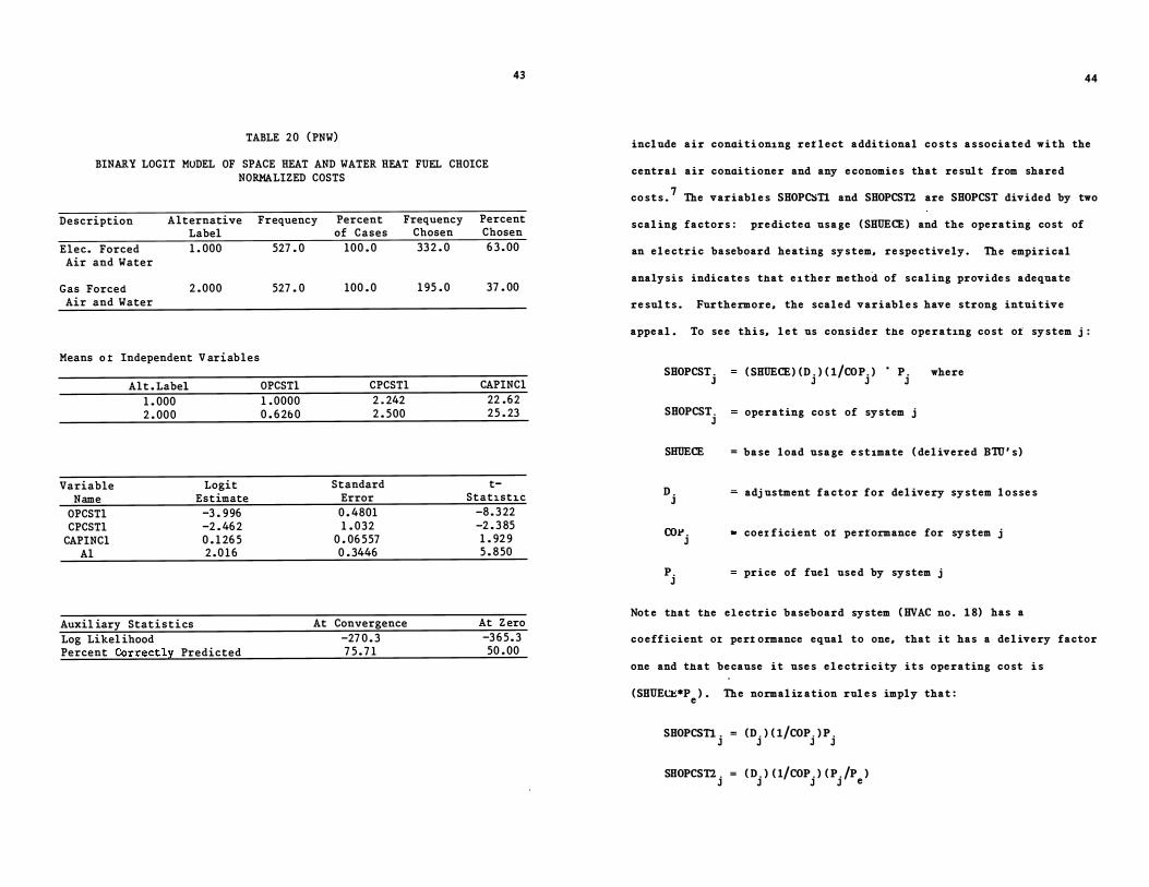
2 . Nested Logit Model o f Spac e H e a t System Choice
The variab l e s SHOPCST and SHCPCST repre sent the operating and
capital cost s of ten alternative HVAC system s . These variabl e s are
calculated using annual predicti ons of usage and capacity deve l oped in
the thermal mode l . Ope rating and capital costs for alterna tives which
43
TABLE 20 (PNW)
BINARY LOGIT MUDEL OF SPACE HEAT AND WATER HEAT FUEL CHOICE NORMALIZED COSTS
Description
Elec. Forced Air and Water
Gas Forced Air and Water
Alternative Label 1 . 000
2 . 000
Frequency
527 . 0
527 . 0
Percent of Cases
100 . 0
100 . 0
Frequency Chosen 33 2 . 0
195 . 0
Means ot Independent V ariables
Variable Name
OPCSTl CPCSTl
CAPINCl Al
Alt . Label 1 . 000 2 . 000
Auxil iary Statistics Log Likel ihood
Logit Estimate
-3 . 996 -2 . 46 2 0 . 1 26 5 2 . 0 1 6
Percent Correctly Predicted
OPCSTl 1 . 0000 0 . 6 2b 0
CPCSTl 2 . 242 2 . 500
Standard Error 0 . 4801 1 . 032
0 . 06 557 0 . 3446
At Convergence -27 0 . 3 7 5 . 7 1
Percent Chosen 6 3 . 00
37 . 00
CAPINCl 22 .62 25 . 23
t-Statistic
-8 . 3 22 -2 . 3 85 1 .929 5 . 850
At Z ero -3 6 5 . 3 50 . 00
44
include air conaitioning retlect additional costs associated with the
central air conaitioner and any economies that result from shared
costs. 7 The variables SHOPC�Tl and SHOPCST2 are SHOPCST divided by two
scaling factors: predictea usage (SHUECE) and the operating cost of
an electric baseboard heating system, respectively. The empirical
analysis indicates that either method of scaling provides adequate
results. Furthermore, the scaled variables have strong intuitive
appeal. To see this, let us consider the operating cost ot system j :
SHOPCST . J
SHOPCST. J
SHUE CE
D . J
CO.I:'. J
P. J
(SHUECE)(D . )(1/COP .) • P . J J J
operating cost of system j
where
= base load usage estimate (delivered B1U's)
adj ustment factor for delivery system losses
coe1 ficient ot pertormance for system j
price of fuel used by system j
Note that the electric baseboard system ( HVAC no. 18) has a
coefficient oI pert ormance equal to one, that it has a delivery factor
one and that because it uses electricity its operating cost is
(SHUE�*Pe). The normalization rules imply that :
SHOPCSTl . = (D . )(1/COP . )P. J J J J
SHOPCST2 . = (D.)(l/COP .)(P./P ) J J J J e
45
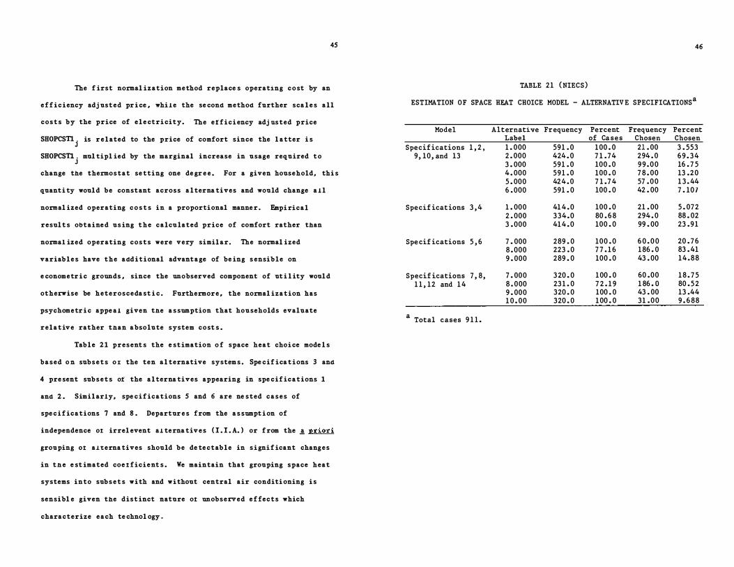
The f irst normal ization method replace s operating c o st by an
e f f i c iency adj usted pr i ce , whi l e the se cond method further sca l e s all
costs by the price of e l e ctri city. The e f f i c i ency adj nsted price
SHOPCS'D. . is r e l ated to the price of comfort since the l atter i s J SHOPCS'D. . mul tipl ied by the marginal increase in usage required t o
J change the thermostat se tting one de gr e e . For a given household, thi s
quanti ty woul d b e constant across a l terna tives and would change a l l
normal ized operating c o s t s in a proportional manne r . Empi rical
resul t s obtaine d us ing the calculated price of comfort rather than
normal ized operating costs were very simil ar. The normal ized
variab l e s have the additional advantage of be ing s ensib l e on
e conometr i c grounds , since the unobserved component of ut i l ity woul d
otherwise be heterosceda st i c . Furthermore , the normal ization has
psychometr i c appe al given tne a s sumption that households evaluate
relative rather tnan absolute system cost s .
Tab l e 2 1 present s the e st imation o f space heat choi ce mode l s
based o n sub s e t s o x the ten al ternative system s . Spe cif ica t i ons 3 and
4 pre sent sub s e t s ot the al terna tives appearing in spe cif ications 1
and 2 . Simil arly, spe c i f ications 5 and 6 are ne sted c a s e s of
spe c i f ications 7 and 8 . Departur e s from the a s sumpt i on of
independence ot irrel event al terna tives ( I . I . A. ) or f rom the .!! priori
grouping ot a1�erna tives should b e de te ctab l e in s i gni f icant changes
in tne e st imated coe t ficient s . We maintain that grouping space heat
systems into sub s e t s with and without central air conditi oning i s
sensibl e given the dist inct nature ot unobserved e f fects which
characterize each te chnol ogy .
46
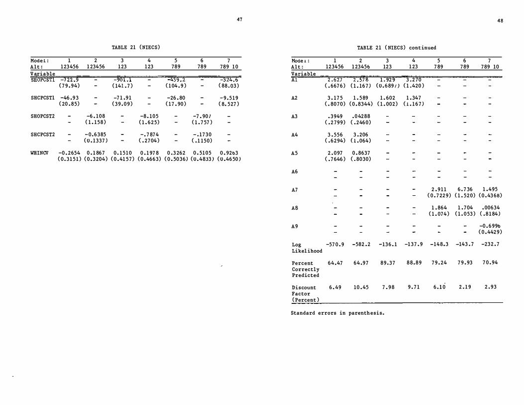
TABLE 21 ( NIECS)
ESTIMATION OF SPACE HEAT CHOICE MODEL - ALTERNATIV E SPECIFICATIONSa
Model Alternative Frequency Percent Frequency Percent Label of Ca ses Chosen Chosen
Specif ications 1 , 2 , 1 . 000 591 . 0 1 00 . 0 21 . 00 3 . 553 9, 10, and 13 2 . 000 424 . 0 7 1 .74 294 . 0 6 9 . 3 4
3 . 000 591 . 0 100 . 0 9 9 . 0 0 16 . 7 5 4 . 000 591 . 0 100 . 0 7 8 . 00 13 .20 5 . 000 424 . 0 7 1 .7 4 57 . 0 0 1 3 . 44 6 . 000 591 . 0 100 . 0 42 . 00 7 . 10 7
Specif ications 3 , 4 1 . 000 41 4 . 0 100 . 0 21 . 00 5 . 072 2 . 000 334.0 80 . 6 8 294 . 0 88 . 02 3 . 000 41 4 . 0 100 . 0 99 . 00 23 . 9 1
Spe cif ications 5 , 6 7 . 000 289 . 0 100 . 0 6 0 . 0 0 20 . 7 6 8 . 000 223 . 0 7 7 . 1 6 1 86 . 0 83 . 41 9 . 000 289 . 0 100 . 0 43 . 00 14.88
Specif ications 7 , 8, 7 . 000 3 20 . 0 1 00 . 0 60 .00 1 8 . 7 5 1 1 , 12 and 1 4 8 . 000 23 1 . 0 7 2 . 1 9 1 86 . o 80 . 5 2
9 . 000 320 . 0 100 . 0 43 . 00 13 .44 1 0 . 00 320 . 0 1 00 . 0 31 . 0 0 9 . 6 88
a Total cases 9 1 1 .
47 48
TABLE 21 ( NIECS) TABLE 21 ( NIECS) cont inued
Mode l : 1 2 3 4 5 6 7 Mooe 1 : 1 2 3 4 5 6 7 Alt : 123 456 1 23456 123 123 789 789 789 1 0 Alt : 123456 1 23456 123 1 23 7 89 7 89 7 89 10 V ariable Variable SHOPCSTl -722.9 - -901.1 - -439. 2 - -3z4.6 Al 2 .627 2 . 578 1 . 92 9 3 . 270
( 7 9 . 94) - ( 141 . 7 ) - ( 1 04 . 9 ) - ( 88 . 03 ) ( . 667 6 ) ( 1 . 16 7 ) ( 0 . 6 89 / ) ( 1 .420 )
SHCPCSTl -46 . 9 3 - -7 1 . 9 1 - -26 . 80 - - 9 . 5 1 9 A2 3 . 17 5 1 . 5 89 1 . 602 1 . 347 ( 20 . 85) - ( 3 9 . 0 9 ) - ( 17 . 90 ) - ( 8. 527 ) ( . 8070) ( 0 . 8344) ( 1 . 002) ( 1 . 1 6 7 )
SHOPCST2 - -6 . 108 - -8 . 105 - -7 . 90 7 - A3 . 3 949 . 0 4288 ( 1 . 1 5 8 ) - ( 1 . 6 25) - ( 1 . 7 57 ) - ( . 2799) ( . 246 0)
SHCPCST2 - - 0 . 6 3 85 - -. 7 874 - - . 17 3 0 - A4 3 . 556 3 . 206 ( 0 . 1337 ) - ( . 27 04) - ( . 1 150) - ( . 6 294) C l . 064)
WHINCV -0 . 2654 0 . 1 867 0 . 1 5 1 0 0 . 1 97 8 0 .3 262 0 . 5105 0 . 92b3 AS 2 . 0 97 0 . 8637 ( 0 . 3 1 5 1 ) ( 0 . 3 204) ( 0 . 41 5 7 ) ( 0 . 4663) ( 0 . 5036) ( 0 . 4833 ) ( 0 .46 50 ) ( . 7 646 ) ( . 8030)
A6 - - - - - - -
A7 - - - - 2 . 9 1 1 6 . 7 36 1 .495 ( 0 . 7 229) ( 1 . 520) ( 0 . 43 68)
AS - - - - 1 . 864 1 . 7 04 . 00634 ( 1 . 074) ( 1 . 0 53 ) ( . 8 1 84)
A9 - - - - - - -0 . 6 99b ( 0 . 4429)
Log -57 0 . 9 -582 . 2 -13 6 . 1 -1 3 7 . 9 -148.3 -143 . 7 -23 2 . 7 Likel ihood
Percent 64.47 64.97 8 9 . 3 7 8 8 . 8 9 7 9 . 24 7 9 . 93 7 0 . 94 Correctly Predicted
Discount 6 . 49 10 . 45 7 . 9 8 9 . 7 1 6 . 1 0 2 . 1 9 2 . 93 Factor ( Percent )
Standard errors in parenthesis.
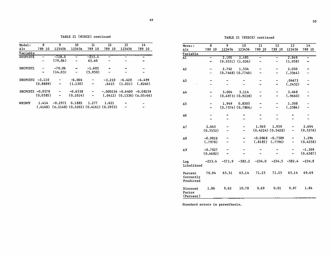
TABLE 21 ( NIECS ) cont inued
Model : 8 9 10 11 12 13 14 Alt 7 89 1 0 1 23 456 123456 789 1 0 789 10 1 23456 789 10 Variable ��F======1�2rllsr:-ou - - 233 •4 SHOPCSTI
( 7 9 . SG ) _ 65 .40
SHCPCSTl -7 0 . 06 ( 14 . 0 3 )
-1 . 603 ( 5 . 9 50)
49
SROPCST2 -3 . 1 1 0 ( 0 . 8889)
-6 . 06 6 ( 1 . 1 3 0 )
- 2 .210 -6 . 420 -4 . 499 . 6415 ( 1 . 03 1 ) ( . 8240 )
SHCPCST2 -0 . 0 57 8 ( 0 . 0 5 85 )
-0 . 6 538 ( 0 . 1014)
- . 000234 -0 . 6 400 -0 . 0 8259 ( . 0412) ( 0 . 1336) C u . 05 1 6 6 )
WHINCV 1 .414 -0 . 2971 0 . 1 883 1 . 277 1 . 621 ( .41 68) ( U . 3 148) ( 0 . 3 203 ) ( 0 . 41 6 1 ) ( 0 . 3 9 5 3 )
TABLE 21 ( NIECS) cont inued
Mocte 1 : 8 9 1 0 11 12 Alt 7 89 10 123456 123456 7 89 10 7 89 10 Variable Al - 2 . 100 2 .485 - -
( 0 . 55 5 1 ) ( 1 . 03 6 ) - -
A2 - 2 . 742 1 . 534 - -( 0 . 7 46 8) ( 0 .7740 ) - -
A3 - - - - -
A4 - 3 . 004 3 . 1 1 4 - -( 0 .497 3 ) ( 0 . 9228) - -
AS - 1 . 949 0 . 8305 - -( 0 . 7 574) ( 0 . 7 80 6 J - -
A6 - - - - -
A7 2 . 045 - - 1 . 56 0 1 . 9 5 9 ( 0 . 5552) - - ( 0 . 4224) ( 0 . 5428)
AS -0 . 9816 - - -0 . 0 86 8 -0 . 7 589 ( . 7 97 8 ) - - ( . 81 85 ) ( . 7796)
A9 -0 .7 027 - - - -( 0 .46 82 ) - - - -
Log -23 3 . 4 -57 1 . 9 -582 . 2 -234 . 0 -23 4 . 5 Likelihood
Percent 7 0 . 94 6 5 . 3 1 6 5 . 1 4 7 1 . 2 5 7 1 .25 Correctly Predicted
Discount 1 . 86 9 . 62 1 0 . 7 8 0 . 6 9 0 . 01 Factor (Percent )
Standard error s in parenthe s i s .
50
13 14 123456 7 89 10
2 . 868 ( 1 . 058)
2 . 030 ( . 3 564)
. 04673 ( . 2452)
3 . 46 8 ( . 9660)
1 . 3 0 8 ( . 2586 )
- -
- 2 . 694 - ( 0 . 5376)
- 1 . 296 - ( 0 . 43 5 8 )
- -1 . 309 - ( 0 .43 87 )
-582 .4 -23 ':1 . 8
6 5 . 1 4 6 9 . 6 9
9 . 97 1 . 84
The re sul ts of the e st imation are quite sensib l e in t erms of
s i gn i f icance and s i gn. Nor do there appear to be any obv ious
departur e s from our sel ected groupings of al ternatives. Without
extensive spe c i f ication te sting it would be diff icult to rej e ct the
a s sumpt i on of I . I . A. or evaluate i t s conse quence s for point
e st imati on. 8
We f ind the inc l us ive value coer f i c i ent to be insi gni f icant
across the vari ous spe c i f i ca t i on. This is not inconsi stent with the
a s sumpt i on of random ut il ity maximiz at i on. It indicate s that
consumers re spond to the maximum uti l ity of possible water heat fue l
al ternatives in the i r se l e ct i on of a space heating sy stem .
51
Given the small di fferent i al in mean water heat inclusive
value across space heat fue l type s , it is l ikely that there i s
s i gnif icant interact i on b e tween the inclusive value variab l e and the
al ternative spe c i f i c dumm i e s . This is further conf irmed by the fact
that the e st imated coe t f ic i ents or operating and capital costs remain
robust even when the incl us ive value coer f i c i ent is constrained to be
z ero ( specif ica t i ons 13 and 14 of Table 21) .
To e xp l or e thi s interact i on hypothe s i s we have e st imated
spe c i fications 9 , 10, 1 1 , 12 in Table 21 . The se mode l s e l imina te the
alternative spe c i f i c effect for oil alternative s . The estimates or
the inclnsive value coer f i c i ent s in spe c i f i ca t i ons 9 and 10 remain
insignificant . However, the hypothe s i s that the est imated inclus ive
value coe f f i c i ent s in the central air conditi oning branch
52
( specif ications 11 and 12 ) equal one cannot be rej ected unde r e i ther
normal ization procedur e . There i s no ..! priori reason to e xpect that
the inclusive value coe t f i c i ent s should differ in the two branches.
Any difference in the two e st imates o f the inclusive value coefficient
could be e xp l i cabl e only by difference s in the degree of intra
correl ations in each space heat cho i ce cluster. The sequential
estimation procedure cannot impo se the constraint that the inclusive
value coef f i c i ent s be equa l . I t i s thus unce rtain whether water heat
cho i ce given spa ce heat cho i ce is the indica ted spe c if icati on. We
therefore adopt the strategy of excl uding the water heat cho i ce
inclusive value in the space heat choice e st imation. The argument i s
that the difference s i n the inclusive value s are small and are
adequately captured in the alternative spe ci f i c e f fect s .
Est imation of di scount f act ors appe ar robust across
spe c i f ications. The di s count f actors are much l ower for the set of
alterna tives that include s a i r conditi oning a s compared with the se t
of alternatives that doe s not include a i r conditi oning . This may be a
refl ect ion 01 shared cost components in a l l-el ectric HVAC syst em s . It
should b e further noted that the se e st imat e s are considerably l ower
than o btains in non-ne sted or binary spe c i f ications ( Hausman ( 1979) ,
Dub in and McFadden ( 19 8� a ) ) .
To e xp l or e the val idity of these conj ectur e s we r e- e st imate
the space heat cho i ce mode l using the Pac i f ic Northwest da ta . Here we
conf ine ourselve s to the f irst six NIECS alterna tive s which do not
include central air-conditioning . Table 22 pre sent s f ive alternative
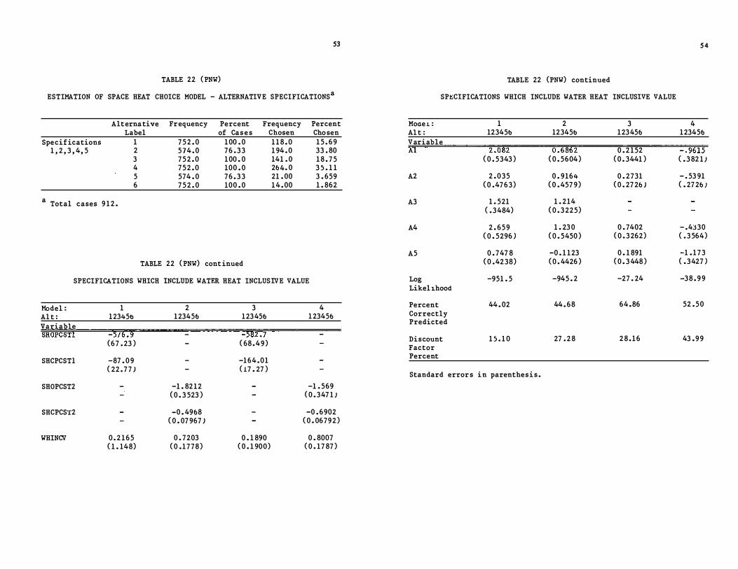
53 5 4
TABLE 22 ( PNW) TABLE 22 (PNW) continued
ESTIMATION OF SPACE HEAT CHOICE MODEL - ALTERNATIVE SPECIFICATIONSa SPt:CIFICATIONS WHICH INCLUDE WATER HEAT INCLUSIVE VALUE
Alternative Frequency Percent Frequency Percent Moae 1 : 1 2 3 4 Label of Cas e s Chosen Cho sen Al t : 12345b 12345b 123 456 123456
Variable Al 2 . 082 0 . 6862 0 . 2 1 52 - . 9615
Specif ications 1 7 5 2 . 0 1 00 . 0 1 1 8 . 0 1 5 . 6 9 1 , 2 , 3 , 4, 5 2 5 7 4 . 0 76 . 3 3 1 94 . 0 33 . 80
3 7 5 2 . 0 1 00 . 0 141 . 0 1 8 . 7 5 ( 0 . 5343 ) ( 0 . 5604) ( 0 . 3441 ) ( . 3 82 1 J 4 7 5 2 . 0 100 . 0 26 4. 0 3 5 . 1 1 5 574 . 0 76 . 3 3 21 . 00 3 . 659 A2 2 . 0 3 5 0 . 9164 0 . 2731 - . 53 91 6 7 5 2 . 0 100 . 0 1 4 . 00 1 . 862 ( 0 .47 6 3 ) ( 0 . 457 9) ( 0 . 27 26 ) ( . 27 26 J
a Total cases 9 1 2 . A3 1 . 521 1 . 214 ( . 3 484) ( 0 . 3 225)
A4 2 . 6 5 9 1 . 23 0 0 . 7402 - .4330 ( 0 . 5296 ) ( 0 . 5450 ) ( 0 . 3 262) ( . 3 564)
AS 0 . 747 8 -0 . 1 1 23 0 . 1 891 -1 . 1 7 3 TABLE 22 ( PNW) cont inued ( 0 .4238) ( 0 . 4426 ) ( 0 . 3 448 ) ( . 3 427 )
SPECIFICATIONS WHICH INCLUDE WATER HEAT INCLUSIVE VALUE Log -951 . 5 -945 . 2 -27 . 24 -3 8 . 9 9 Likel ihood
Percent 44 . 02 44 . 6 8 64.86 52 . 5 0 Correctly Predicted
Model : 1 2 3 4 Al t : 12345b 123456 123 456 1 23456 Variable
Discount 1 5 . 1 0 27 . 2 8 2 8 . 1 6 43 . 9 9 Factor
SHOPCSTl -516.9 - -582 .7 ( 6 7 . 23 ) - ( 68 . 4 9 )
Percent SHCPCSTl -87 . 0 9 - -164.01
Standard error s in parenthes i s . ( 22 . 7 7 ) - ( 17 . 27 )
SHOPCST2 - -1 . 8212 - -1 . 569 ( 0 . 3 523 ) - ( 0 . 3 47 1 J
SHCPCST2 - -0 . 4968 - -0 . 6 902 ( 0 . 07 967 ) - ( 0 . 06792)
WHINCV 0 . 2 1 6 5 0 . 7203 0 . 1 890 0 . 8007 ( 1 . 148) ( 0 .1778) ( 0 . 1 900) ( 0 . 17 87 )
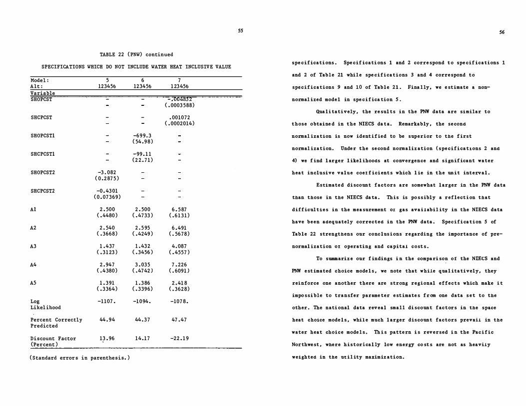
TABLE 22 ( PNW) continued
SPECIFICATIONS WHICH DO NOT INCLUDE WATER HEAT INCLUSIVE VALUE
Model : 5 6 7 Alt : 123456 123456 1 23 456 Variable SHOPCST - - -.004832
( . 0003 588)
SHCPCST - - . 001072 ( . 0002014)
SHOPCSTI - -6 9 9 . 3 ( 54 . 9 8 )
SHCPCSTI - -99 . 1 1 ( 2 2 . 7 1 )
SHOPCST2 -3 . 082 ( 0 .287 5 )
SHCPCST2 -0 . 43 01 ( 0 . 07 3 6 9 )
Al 2 . 500 2 . 500 6 . 5 87 ( . 4480 ) ( . 4733 ) ( . 6 1 3 1 )
A2 2 . 540 2 . 5 95 6 . 491 ( . 3668) ( . 4249 ) ( . 5678)
A3 1 . 437 1 . 43 2 4. 087 ( . 3 1 23 ) ( . 3456 ) ( . 4557 )
A4 2 . 947 3 . 03 5 7 . 226 C . 4380 ) ( . 4742 ) ( . 6091 )
AS 1 . 3 91 1 . 3 86 2 . 41 8 ( . 3364) ( . 3396) C . 3628)
Log -1107 . -1 0 94 . -107 8 . Likel ihood
Percent Correctly 44 . 94 44 . 3 7 47 . 47 Predicted
Discount Factor 13 . 96 14.17 -22 . 1 9 (Percent )
-
( Standard error s in parenthe s i s . )
55 56
spe c i f icati ons . Spe cif icati ons 1 and 2 corre spond t o spe cif ications 1
and 2 of Tab l e 21 whil e spe c i f i cations 3 and 4 corre spond t o
spe c i f ications 9 and 10 of Tab l e 21 . Fina l ly, we e stimate a non-
normal ized mode l in spe c i f ica tion 5 .
Qua l i tatively, the re sul ts in the PNW data are similar to
those obtaine d in the NIECS da ta. Remarkably , the se cond
normal ization is now ident i f ied to be superior to the f irst
normal ization. Unde r the se cond normaliz ation ( spe c i f i cations 2 and
4) we f ind l arger l ikel ihoods at convergence and signif icant water
heat inclusive valne coet f ici ent s which l ie in the unit interval .
Estimate d di scount f actors are somewhat l arger in the PNW data
than those in the NIECS da ta . This is po ssibly a reflect i on that
diff icul t i e s in the mea surement 01 gas ava i l abil ity in the NIECS data
have b e en adequately corrected in the PNW data . Spec i f i cation 5 of
Tab l e 22 strengthens our conc lus i ons regarding the importance of pre-
normal ization 0 1 operating and capital cost s .
To s1lllllllariz e our f indings i n the compari son o f the NIECS and
PNW e st imated choice mode l s , we note that while qual itatively, they
reinforce one another there are strong regional effects which make i t
impo ssible to transfer parame ter e st imate s f r om one data s e t to the
other . The nati onal data reveal sma l l di scount f actor s in the space
heat choice mode l s , whil e much l arger discount factors prevail in the
water heat choice mode l s . Th i s patte rn i s reversed i n the Pac i f ic
Northwe st , where histor i cal ly low energy co st s are not as heavily
weighted in the ut i l ity maximiz ation.
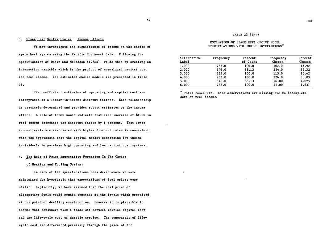
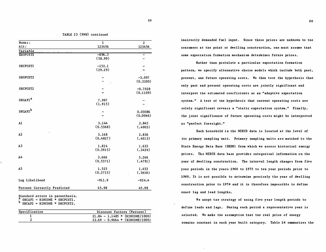
3 . Space Heat Sys tem Cho ice - Income Effects
57
We now invest i ga te the s i gnificance of income on the choice of
space heat system using the Pac i f ic Northwest data . Fol l owing the
spe c i f ication of Dubin and McFadden ( 19 83 a) , we do thi s by creating an
interact i on variab l e which i s the product of normal ized capital cost
and real income . The e st imate d choice mode l s are pre sented in Tab l e
23 .
The coeff i c i ent e st imate s of operating and capital cost are
interpreted as a l inear- in- income dis count factor s . Each rel at1onship
is preci sely de termine d and provide s robust e st imates ot the income
effec�. A rule-of-thumb would indicate that e ach increase of ilOOO in
real income de crease s the discount f actor by 1 percent . That l ower
income l eve l s are associated with higher di scount rate s is consi stent
w ith the hypothe s i s that the capital marke t constrains l ow income
individua l s to purchase high operating and l ow capi tal cost sy stem s .
4 . The Rol e o f Price Expectat ion Formation In The Cho i c e
o f Heat ing and Cool ing Systems
In e ach of the spe c i f ications consi dered above we have
maintaine d the hypothe s i s that e xpe ctations of fue l pri ce s were
st a t i c . Imp l i c i tly, w e have a s sumed that the r e a l pri ce o f
alternat1ve fue l s would remain constant a t the l evels which pr evailed
a t the po int ot dwe l l ing construc t i on. Howeve r i t i s pl ausible to
a s sume that consumers v i ew a trade-off be tween ini t i al capital c o st
and the 1 ife-cycle cost or durable serv ice . The component s of l ife-
cyc l e cost are determined primarily through the price of the
Alternative Label 1 . 000 2 . 000 3 . 000 4. 000 5 . 000 6 . 000
TABLE 23 (PNW)
ESTIMATION OF SPACE HEAT CHOICE MODEL SPECIHCATIONS WITH INCOME INTERACTIONSa
Frequency Percent Frequency of Case s Cho sen
733 . 0 100 . 0 102 . 0 646 . 0 8 8 . 1 3 254 . 0 733 . 0 100 . 0 1 1 3 . 0 733 . 0 100 . 0 226 . 0 646 . 0 88 . 1 3 26 . 00 733 . 0 1 00 . 0 1 2 . 00
5 8
Percent Cho sen 13 . 92 3 9 . 3 2 1 5 . 42 3 0 . 83 4. 025 1 . 637
a Total cases 9 1 2 . Some observations are missing due to incomplete data on real income.
5 9
TABLE 2 3 ( PNW) cont inued
Mode l : Alt : Variable SHOPCSTl
SHCPCSTI
SHOPCST2
SHCPCST2
SHCAPl a
SHCAP2b
Al
A2
A3
A4
AS
Log Likel ihood
Percent Correctly Predicted
Standard errors in parenthe s i s . � SHCAPl = RINCOME * SHCPCSTI . SHCAP2 = RINCOME * SHCPCST2 .
S�ecif ication I 2
I 123456
-696 . 3 ( 58 . 99 )
-1 52 . 1 ( 29 . 2 9 )
-
-
7 . 997 ( 1 . 9 1 5 )
-
3 . 144 ( 0 . 5368)
3 . 16 8 ( 0 . 4827 )
1 . 814 ( 0 . 391 5 )
3 . 666 ( 0 . 53 7 1 )
1 . 525 ( 0 . 3 7 1 5 )
-91 1 . 9
45 . 98
2 123456
-3 . 0 97 ( 0 . 3 100)
-0 . 7 028 ( 0 . 1 1 09)
0 . 03086 ( 0 .0066)
2 . 845 ( . 4903 )
2 . 836 ( . 401 3 )
1 . 633 ( . 343 9 )
3 . 266 ( . 47 91 )
1 .453 ( . 3650 )
-924.4
45 . 9 8
Discount Factors (Percent ) 21 . 84 - 1 . 1 485 * (RINCOME / 1 000) 22.69 - 0 . 9664 * (RINCOME/ 1 000)
60
inairectly demanded fue l input . Since these pri ce s are unknown to the
consumers a t the point or dwe l l ing construction, one must a ssume that
some expectation formation me chani sm de termine s future price s .
Rather than po stul ate a particul ar exp e ct ation formati on
patte rn, we spe c i fy alternative choi ce mode l s which include both past ,
present , and future operating c o st s . We then t e st the hypo the s i s that
only past and pre sent operating costs are j ointly s i gnif icant and
interpret the e st imated coex f i ci ent s as an " adaptive expe ctation
system . " A t e st ol the hypothe s i s that current operating c o st s are
sol ely s i gni f i cant revea l s a " st a t i c e xpe ctation system . " Fina l ly ,
the j oint s i gni f icance of future ope rating c o s t s m i ght be interpreted
a s "perf ect f or e s i ght . "
Each household i n the NIECS data i s located a t the l evel of
its primary sampl ing uni t . Primary sampl ing uni t s a r e matched t o the
State Ene rgy Dat a Base ( SEDS) from which we acce s s hist or i cal ene r gy
pri ce s . Th e NIECS data base prov ide s cate gori cal information o n the
year of dwel l ing constructi on. The interval l ength change s from f ive
year periods in the years 1 960 to 1975 to ten year periods pri or to
1 960 . It i s not possible to de termine preci sely the year of dwe l l ing
construction prior to 1974 and it is therefore impo s sibl e to def ine
exact l ag and l ead l ength s .
W e adopt t h e strategy of using f ive y e a r l ength periods to
de f ine l eads and l ags . During e ach pe riod a repre sentative year i s
s e l e cted. We make the a s sumpt i on that the real pri ce o f energy
remains constant in each year bui l t cate gory. Tab l e 24 summari z e s the
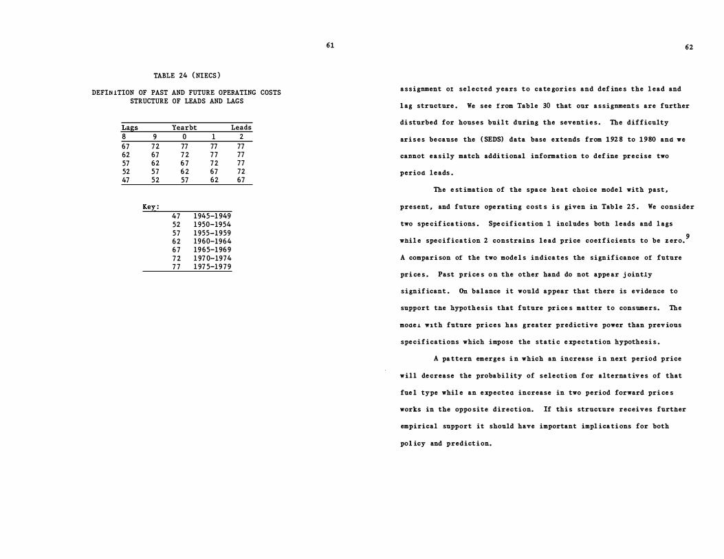
TABLE 24 ( NIECS )
DEFIN lTION OF PAST AND FUTURE OPERATING COSTS STRUCTURE OF LEADS AND LAGS
Lags 8 67 62 57 52 47
9 72 67 62 57 52
Key:
Yearbt Leads
47 52 57 6 2 6 7 7 2 7 7
0 77 7 2 6 7 6 2 57
1 77 77 72 67 62
1 945-1 949 1 950-1954 1 955-1 959 1960-1964 1965-1 96 9 1 97 0-1974 1 97 5-1 9 7 9
2 77 77 77 72 67
61 62
assignment ot sel ected years t o cate gor i e s and def ine s the l ead and
l ag structure . We see f rom Table 30 that our a s s i gnment s are further
di sturbed for hous e s bui l t during the sevent i e s . The difficulty
ari s e s be cause the ( SEDS) data base extends from 1 92 8 to 1 9 80 and we
cannot e a s i ly match addi tional information to def ine pre c ise two
period l e ads .
The e st imation of the spa ce heat choi ce mode l with past ,
present , and future ope rating cost s i s given in Tab l e 25 . We cons i de r
two spe cif ica tions . Spe cification 1 include s both l eads and l ags
whil e spe c i f icati on 2 constrains l e ad pri ce coet f i ci ents to be z ero.9
A compari son of the two mode l s indica tes the significance of future
pri ce s . Past pri ce s o n the other hand do not appe ar j ointly
signif icant . On bal ance it would appear that there is evidence to
support tne hypoth e s i s that future pri ce s matter to consumers. The
mooe � with future pri c e s has greater predictive power than prev ious
spe c i f i cati ons which impose the stati c e xpectation hypothesi s .
A pa ttern emerge s i n which an increase i n next period price
will de crease the probabi l ity of s e l e ct i on f or alterna t iv e s of that
fue l type whil e an e xpecteo increase in two period forward pri ce s
works in the oppo site directi on. If thi s structure receives further
empirical support it should have important impl icati ons for both
pol icy and predict i on.
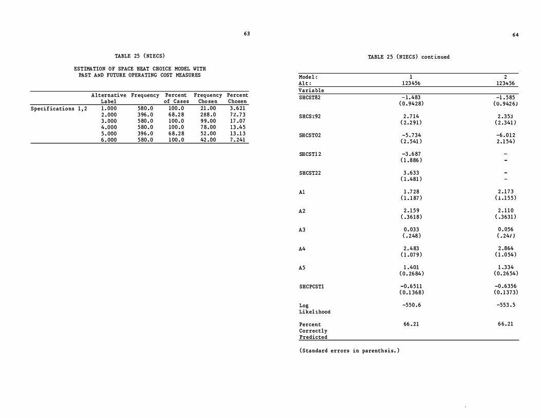
TABLE 25 ( NIECS)
ESTIMATION OF SPACE HEAT CHOICE MODEL WITH PAST AND FUTURE OPERATING COST MEASURES
63
Alternative Frequency Percent Frequency Percent Label of Cases Cho sen Chosen
Specif ications 1 , 2 1 . 000 580 . 0 100 . 0 21 . 00 3 . 6 21 2 . 000 3 96 . 0 6 8 . 2 8 288 . 0 1 "1. . 7 3 3 . 000 5 80 . 0 100 . 0 9 9 . 00 17 . 07 4 . 000 5 80 . 0 100 . 0 7 8 . 00 13 .45 5 . 000 396 . 0 6 8 . 28 52 . 00 13 . 1 3 6 . 000 5 80 . 0 1 00 . 0 42 . 00 7 . 241
Model : Al t : Variable SHCST82
SHCST92
SHCST02
SHCST1 2
SHCST22
Al
A2
A3
A4
AS
SHCPCSTl
Log Likel ihood
Percent Correctly Predicted
TABLE 25 (NIECS) cont inued
1 123 45()
- 1 . 483 ( 0 . 9428)
2 . 7 14 ( 2 . 2 91 )
-5 . 734 ( 2 . 541 )
-3 . 6 87 ( 1 . 886 )
3 . 633 ( 1 .481 )
1 .7 28 ( 1 . 1 87 )
2 . 1 5 9 ( . 3 6 1 8 )
0 . 033 ( . 248 )
2 . 483 ( 1 . 07 9 )
1 . 401 ( 0 . 26 84)
-0 . 6 511 ( 0 . 1 368)
-550 . 6
66 . 21
( Standard errors in parenthsis. )
64
2 123456
-1 . 5 85 ( 0 . 942 6 )
2 . 3 S;j ( 2 .341 )
-6 . 0 1 2 2 . 1 54)
2 . 1 7 3 ( ! . 1 5 5 )
2 . 1 1 0 ( . 3 631 )
0 . 056 ( . 24/ J
2 . 864 ( 1 . 0 54)
1 .334 ( 0 . 26 54)
-0 . 6356 ( 0 . 1 373)
-553 . S
6 6 . 21
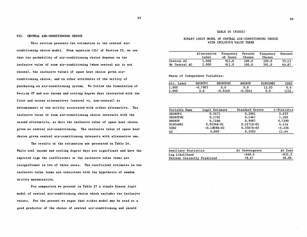
6 5
VII . CENTRAL AIR-CONDITIONING CHOICE
Thi s s e c t i on presents the e st imation ot the central air-
conditioning choi ce mode l . From equation ( ll J of Sect i on II, we see
that the probab il ity of air-conditi oning choice depenas on the
inclusive value of room air-conditi oning ( when central air is not
chosen) , the inclusive value s of space heat choi ce given a i r-
conditioning choi ce , and o n other attribute s o f the ut i l ity o f
purchasing a n ai r-conaiti oning sy stem . W e fol l ow the formul ation o f
Section IV and u s e income and cool ing degree days interacted with the
f irst and se cona a l terna tive s ( central vs . non-centr al ) a s
determinant s oI the ut i l ity associ ated with e i ther alterna tiv e . Th e
inclusive value of room air-conaiti on1ng choi ce interacts with the
se cond al terna tive, as doe s the inclusive value of space heat choice
given no central air-conaiti on1ng . The inclusive value of space heat
cho i ce given central ai r-conaitioning interact s with alternative one .
The re sul ts of the e st imation are pre sented in Tab l e 2 6 .
Whi l e real income and cool ing degr e e days are s i gni f icant and have the
exp e cted s i gn the coefficient s ot the inclusive value terms are
insignificant in two of thre e case s . The coe t f i c i ent e st imates on the
inclus ive value terms are cons i st ent w ith the hypothe s i s of random
ut il ity maximiz ation.
For comparison we present in Tab l e 27 a simple binary logit
mode l of central ai r-conditioning choi ce which exc l ude s the inclus ive
valne s . For the present w e argue that e i ther mode l may be u s e d a s a
good predictor of the choice of central air-conditioning and shoul d
TABLE 26 ( NIECS )
BINARY LOGIT MODEL OF CENTRAL AIR-CONDITIONING CHOICE WITH INCLUSIVE VALUE TERMS
Al ternative Label
Central AC 1 . 000 No Central AC 2 . 000
Frequency of Cases
911 . 0 91 1 . 0
Means o f Independent V ariabl e s :
Al t . Label 1 . 000 2 . 000
SHINCVC -0 . 7 90 5
0 . 0
SHIN CV NC 0 . 0
-0 . 91 6 0
Percent Chosen 100 . 0 100 . 0
RMINCV 0 . 0
-0 . 5041
Frequency Cho sen 3 20 . 0 591 . 0
RINCOMEl 1 2 . 03
0 . 0
66
Percent
3 5 . 1 3 64.87
CDD2 o . o
1 1 21 .
Variable Name Logit Estimate Standard Errors t-Statistic SHINCV C SHIN CV NC RMINCV RINCUMEl CDD2 A2
Auxil iary Statistics Log Likel ihood
0 . 5471 0 . 1 7 01 0 . 7280
0 . 93 54E-01 -0 . 1 80 8E-02
4.009
Percent Correctly Predicted
0 . 2061 0 . 1 467 0 . 9987
0 . 2271E-01 0 . 5587E-03
0 . 3 503
At Convergence -449 . 4 7 8 . 27
2 . 6 5 5 1 . 160
0 . 7 290 4 . 1 1 !!
-3 . 23 6 1 1 .44
At Z ero -631 . 5 50 . 00
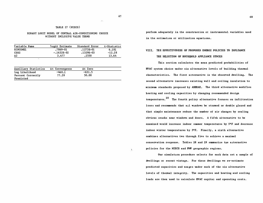
TABLE 27 ( NIECS )
BINARY LOGIT MODEL OF CENTRAL AIR-CONDITIONING CHOICE WITHOUT INCLUSIVE VALUE TERMS
67
V ariable Name Logit Estimate Standard Error t-Statistic RINCOMEl CDD2 A2
Auxil iary Statistics Log Likel ihood Percent Correctly Predicted
• 7 869-01 - . 1 632E-02
3 .47 7
A t Convergence -46 0 . 1 77 . 3 9
. 1 273E-01
. 1 329E-03 . 2550
At Zero -63 1 . 5 50 . 00
6 . 1 81 -1 2 . 2 8 13 .64
6 8
perform adequately i n the construct ion or instrumental. variab l e s used
in the est imation or ut i l ization equations .
VII I . TH E EFFECTIVENESS OF PROPOSED ENERGY POLICIES TO INFLUENCE
THE SELECTION OF HOUSEHOLD APPLIANCE STOCKS
Thi s section calculate s the mean predicted probab i l i t i e s of
HVAC system choice under six al ternative l evel s of bui l ding thermal
charact eri st i c s . The f irst alternative is the ob served dwe l l ing . The
se cond alternative increase s exist ing wal l and c e i l ing insul ation to
minimum standards propo sed by ASHRAE . The third alternative modi f i e s
heating and cool ing capa c i t i e s b y changing r ecommended de s i gn
temperatur e s .10
The fourth pol icy al ternative focus e s on infil trati on
l ose s and recommends that a i l windows be stormed or doub l e glazed and
that simpl e maintenance reduce the number of air chang e s by seal ing
obvious cracks near w indows and door s . A f if th al ternative to be
examine d would increase indoor summer tempe ratur e s by S°F and decrease
indoor w inter tempe ratures by S°F. Fina l ly , a sixth alterna tive
comb ine s al ternatives two through f ive to achieve a maximal
conservation r e sponse . Tabl e s 28 and 29 summari z e tne a1ternative
po l ic i e s for the NIECS and PNW geographic regi ons .
Our simul ation proce dure se l e c t s for each data set a sample of
dwe l l ings or recent vintage . For these dwe l l ings we re-estimate
predicted capa c i t i e s and usa ge s under each of the six alternative
l evel s of thermal inte grity. The capa c i t i e s and heating and cool ing
l oads are then used to cal cul ate HVAC capital and operating c o st s .
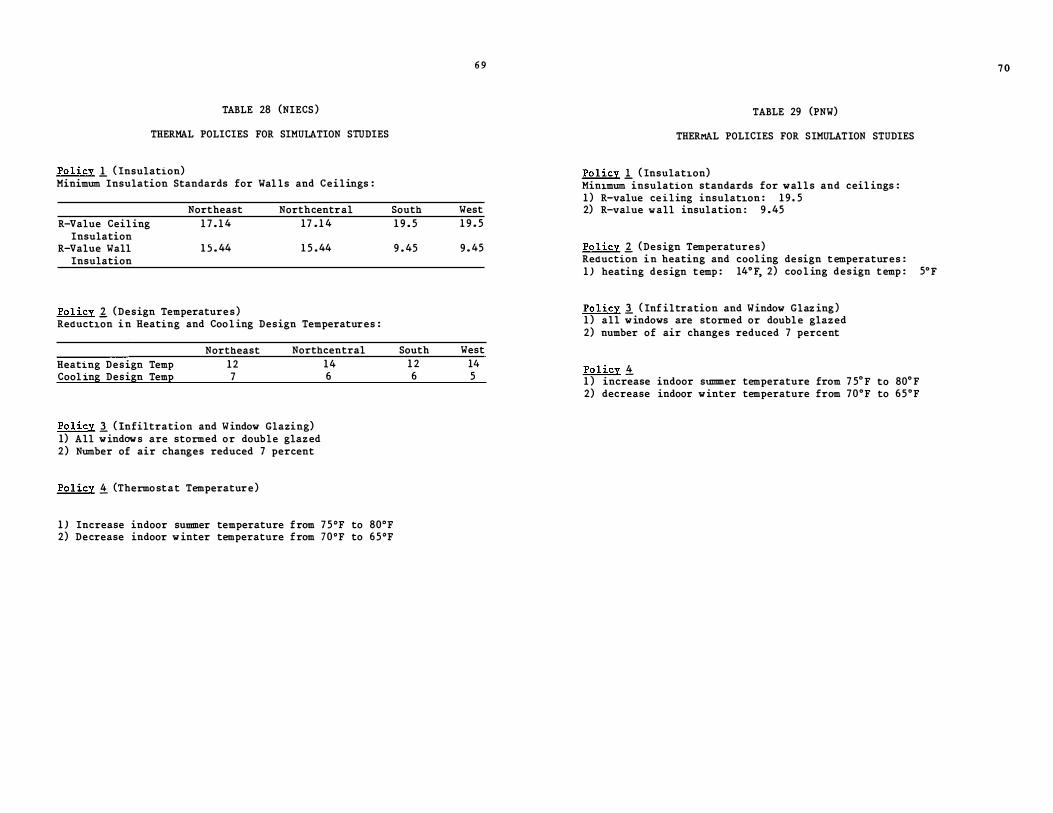
TABLE 28 (NIECS )
THERMAL POLICIES FOR SIMULATION STUDIES
Po licy .!. ( Insulation) Minimum Insulation Standards for Wal ls and Ceilings :
Northeast North central South R-Value Ceil ing
Insulation R-Value Wall
Insulation
1 7 . 1 4 17 . 1 4
1 5 . 44 1 5 . 44
Pol icy 1. (Design Temperature s ) Reduction i n Heating and Coo l ing Design Temperatures :
Northeast Northcentral Heating Design Temp Cool ing Design Temp
12 7
Pol icy .1 ( Infiltration and Window Glazing) 1) All w indow s are stormed or double glaz ed 2) Number of air changes reduced 7 percent
Po l icy ! (Thermo stat Temperature)
14 6
1 ) Increase indoor summer temperature from 7 5 °F to 80°F 2) Decrease indoor w inter temperature from 70°F to 6 5 °F
1 9 . 5
9 . 45
South 1 2 6
6 9
West 1 9 . 5
9 . 45
West 14 5
TABLE 29 (PNW)
THERMAL POLICIES FOR SIMULATION STUDIES
Pol icy .!. ( Insulation) Minimum insulation standards for wal l s and ceil ings : 1 ) R-value ce iling insulation : 1 9 . 5 2) R-value wall insulation : 9 . 45
Policy 1. (Design Temperatures) Reduction in heating and cool ing de sign t emperatures : 1 ) heating design temp : 14° F, 2) coo l ing design temp : 5°F
Po l icy .1 ( Inf iltration and Window Glaz ing ) 1 ) all w indows are stormed or doubl e glaz ed 2) number of air changes reduced 7 percent
Pol icy ! 1 ) increase indoor summer temperature from 7 5° F to 80° F 2) decrease indoor w inter temperature from 70°F to 65°F
7 0
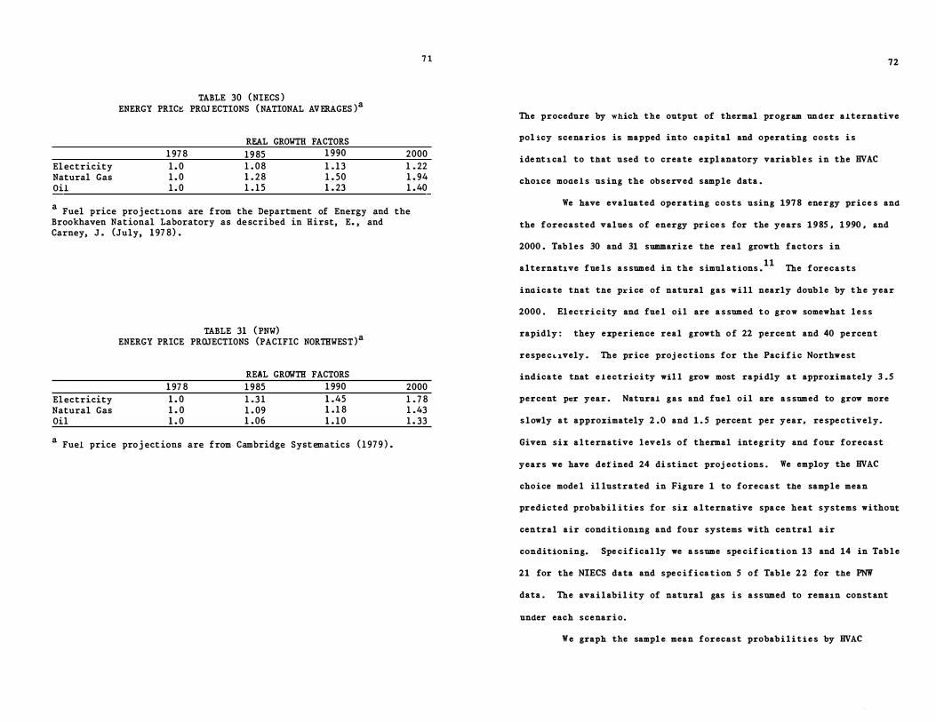
El ectricity Natural Gas Oil
TABLE 30 ( NIECS ) ENERGY PRIC� PROJ ECTIONS ( NATIONAL AVERAGES )a
1 97 8 1 . 0 1 . 0 1 . 0
REAL GROWTH FACTORS 1 9 85 1 990 1 . 0 8 1 . 28 1 . 1 5
1 . 13 1 . 50 1 . 23
7 1
2000 1 . 22 1 . 94 1 . 40
a Fuel price proj ections are from the Department of Energy and the Brookhaven National Laboratory as de scribed in Hirst, E. , and Carney, J . (July, 1 97 8) .
El ectricity Natural Gas Oil
TABLE 31 ( PNW) ENERGY PRICE PROJECTIONS (PACIFIC NORTHWEST)a
1 97 8 1 . 0 1 . 0 1 . 0
REAL GROWTH FACTORS 1 985 1 990 1 . 3 1 1 . 45 1 . 09 1 . 1 8 1 . 06 1 . 1 0
a Fuel price proj ect ions are from Cambridge Syst ematics ( 1 97 9 ) .
2000 1 . 7 8 1 . 43 1 . 33
72
The procedure by which the output of thermal program under alternative
pol icy scenarios is mapped into capital and operating costs i s
i de nt i cal to that used t o create expl anatory variabl e s in the HVAC
choice moae l s us ing the observed sample data .
We have evaluated operating costs using 197 8 ene r gy price s and
the forecasted value s of energy pri ce s for the years 1 9 85 , 1 990 , and
2000 . Tab l e s 30 and 31 summari z e the real growth factors in
alternative fue l s a s sumed in the s imul ations .11
The f orecasts
inaicate tnat tne pr i ce of natural gas w i l l nearly doub l e by the year
2000 . El ecrri city and fue l oil are a s sumed t o grow somewhat l e s s
rapidly : they experience real growth o f 22 perce nt and 40 pe rcent
respe c . 1vely . The price proj e c t i ons for the Pac i f i c Northwest
indicate tnat e l ectricity wil l grow most rapi dly at approximately 3 . 5
percent per year . Natural gas and fue l o i l are a s sumed to grow more
s l owly at approximately 2 . 0 and 1 . 5 percent per year, re spe ctively.
Given six alternative l evels o f thermal integrity and f our forecast
years we have def ined 24 di st inct proj ections . We employ the HVAC
cho i ce mode l il lustrated in Figure 1 to forecast the sample mean
predicted probab i l i t i e s for six a l te rnative spa ce heat systems without
central air conditi oning and four systems with central air
conditioning. Spe c i f ical ly we a ssume spe cif ica t i on 13 and 14 in Tab l e
21 for the NIECS data and spe c i f i ca t i on 5 o f Table 2 2 for the PNW
data . The ava i l abil ity of natural gas i s a ssumed to remain constant
under each scenar i o .
W e graph the sampl e mean forecast probab i l i t i e s by HVAC
73
alternative, po l icy scenario, and forecast year in Fi gure 2 . For each
HVAC alternative a corre sponding graph in Fi gure 2 prov ide s scale
information and an i dentif ication of each plotted curv e . Th e l abel s
for each alternative are e a s i ly found in Figure 1 or Tabl e 17 .
In tne NIECS data we see an increase in e l ectric force d a i r
and e l ec .r i c ba seboard sy stem s . Conservation po l ic i e s, however, coul d
de crease the overal l share oI e l e ctric forced air systems while
incr e a sing the snare ot el ectric ba seboard systems rel ative to current
standards .
Gas systems reveal de crea se s in overal l saturations .
Conservation po l ic i e s appe ar to reinforce thi s effect by further
reducing predicted m arke t snare s . Oil al ternative s snow a mode rate
de crea se in market share by 1 9 85 whi l e the overal l trend is to
increase marke t share s l ightly from 3 to 6 percent. Conservation
pol i c i e s wil l de crease the prevalence of thi s alternat iv e - by the year
2000 . This pattern continue s t o hold in system s with air
conditioning . Intere stingly, e l ectric heat pumps, which are forecast
to enj oy an increa sing market share in new construction and
conservation po l i c i e s , wil l re inforce this pattern.
In the Pac i f ic Nortnwest e l ectric systems are forecast t o gain
rel ative to other fue l type s . However el e ctri c ba seboard systems
ini t i al ly increase and then decrease in m arke t snare as e l ectri city
price s reach rel atively high l evel s in the year 2000 . Ga s forced air
sy stems are fore cast to de crease in prevalence ana conservation
pol ici e s w i l l strenghten thi s trend. Oil heating sy stems , which have
rel atively l ittle market share in the Pac i f i c Northwest, are not
reveal ed to demonstrate l arge change s in the ir pene tration.
The propo sed ASHRAE standards woul d appe ar to generally
increase the snare s ot energy ef ficient heating and cool ing system s .
Forecasts f o r actual ene r gy usage which re sul t unde r al terna tive
conservation scenarios w i l l be reported e l sewhere .
7 4
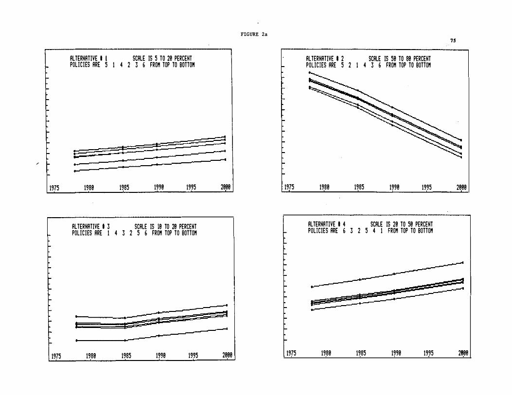
/
1975
1975
ALTERNATIVE I I SCALE IS 5 TO 20 PERCENT POLICIES ARE 5 I 4 2 3 6 FROM TOP TO BOTTO"
�:...-....... ....-��-
1980 1985 1999 1995
ALTERNATIVE I 3 SCALE IS 10 TO 20 PERCENT POLICIES ARE I 4 3 2 5 6 FROM TOP TO BOTTOM
1980 1985 1990 1995
__, -4
�
2000
2000
FIGURE 2a
1975
1975
ALTERNATIVE I 2 SCALE IS 50 TO 80 PERCENT POLICIES ARE 5 2 I 4 3 6 FROM TOP TO BOTTOM
1980 1985 1999 1995
ALTERNATIVE I 4 SCALE IS 20 TO 50 PERCENT POLICIES ARE 6 3 2 5 4 I FROM TOP TO BOTTOM
....-
1980 1985 1990 1995
75
2990
2909
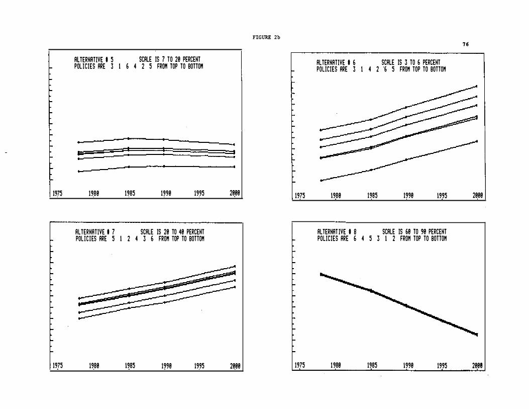
1975
1975
RLTERNRTIYE I 5 SCALE IS 7 TO 20 PERCENT POLICIES ARE 3 l 6 4 2 5 FRO" TOP TO BOTTO"
Iii - ===I
1980 1985 1990 1995
RLTERNRTIYE I 7 SCALE IS 20 TO 40 PERCENT POLICIES ARE 5 l 2 4 3 6 FROM TOP TO BOTTOM
1980 1985 1990 1995
2000
2000
FIGURE 2b
.---���������������������-'
1975
1975
ALTERNATIVE I 6 SCALE IS 3 TO 6 PERCENT POLICIES ARE 3 l 4 2 "6 5 FROM TOP TO BOTTOM
1980 1985 1990 1995
ALTERNRTIYE I 8 SCALE IS 60 TO 90 PERCENT POLICIES ARE 6 4 5 3 l 2 FROM TOP TO BOTTOM
1980 1985 1990 1995
7 6
2000
2008
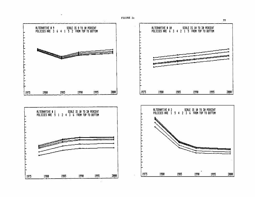
1975
1975
ALTERNATIVE I 9 SCALE rs 8 TO 10 PERCENT POLICIES ARE 3 6 4 1 5 2 FRO" TOP TO BOTTO"
1980 1985 1990 1995
ALTERNATIVE I I SCALE IS 10 TO 30 PERCENT POL ICIES ARE 5 1 2 4 3 6 FROM TOP TO BOTTOM
2000
e��=------- -- - -���
1980 1985
I I
1990 1995 2000
FIGURE 2c
1975
1975
ALTERNATIVE • 10 SCALE rs 10 TO 30 PERCENT POLICIES ARE 6 3 4 2 I 5 FROM TOP TO BOTTOM
77
______ __,..
;::,....-
1980 1985 1990 1995
ALTERNATIVE I 2 SCALE IS 10 TO 30 PERCENT POLICIES ARE 1 5 4 2 3 6 FROM TOP TO BOTTOM
1980 1985 1990 1995
2000
2000
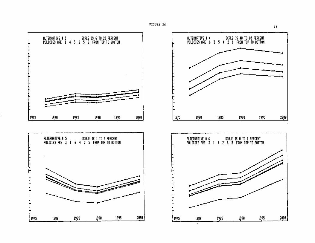
1975
1975
ALTERNATIVE I 3 SCALE IS 6 TO 20 PERCENT POLICIES ARE l 4 3 2 5 6 FRO" TOP TO BOTTO"
�·· = :::::::-==
1988 1985 1998 1995
ALTERNATIVE I 5 SCALE IS l TO 3 PERCENT POLICIES ARE 3 l 6 4 2 5 FRO" TOP TO BOTTO"
1980 1985 1990 1995
2008
2000
FIGURE 2d
1975
1975
ALTERNATIVE I 4 SCALE IS 40 TO 60 PERCEHT POLICIES ARE 6 3 5 4 2 I FROM TOP TO BOTTO"
1980 1985 1990 1995
ALTERNATIVE I 6 SCALE IS 0 TO I PERCENT POL ICIES ARE 3 l 4 2 6 5 FRO" TOP TO BOTTO"
1980 1985 1998 1995
7 8
2000
2808
7 9
F001NOTES
1 . The author acknowledge s the r e se arch assi stance of Paul Bj orn who
a i de d in the simul ation e xp e riments ot s e c t i on VIII. He further
thanks Phi l ip Hoffman and Steven Hensen for reading and
comment ing on a prel iminary draf t .
2 .
3 .
See Goett ( 1 9 82 ) for an example of thi s approach .
The incl us iv e value coe t f i c i ent i s de f ine d ana interpr eted in
McFadden ( 19 83 ) .
4 . Th e NIECS data provide information about the nlllD.ber ox room air
conditi one r s owne d by the household ana the nlllD.ber ox rooms air
conditione d but no information i s avail ab l e on individual room
air cona i t i oner et f ici ency . Estimation i s conf ined to the NIE�S
data a s a i r conaiti on1ng i s not an important consi de ration in tne
Pac i f ic Northwest .
S . The thermal model of Dub in and McFadden ( 19 83b ) prov ide s direct
e stimate s o f air conditi oning de sign capa c i ty given hous ehol d
charact e r i s t i cs and location spe ci f i c temperature informati on.
6 . The sample i s additi onally edited t o e l imina te inf requently
s e l e c� e d space heating system s . This point wil l be taken up
b e l ow.
80
7 . For de tai l s tne reader i s referred to Cow ing , Dubin, and McFadden
( U 81 e ) .
8 . McFadden, Tye , and Train ( 197 8) and Hausman and McFadden ( 19 82 )
di scus s two t e s t s ox the I . I . A. property.
9 . Normal ization method two i s used in the e st imation of
spe cif ications 1 and 2 .
1 0 . Dubin and McFadden ( 1 9 8jb ) di scus s de ta i l s of the ASHRAE thermal
standards and the conne c t i on between de s i gn temperature and HVAC
capacity.
11 . We a ssume that the real pr i ce of capi tal goods and household
demographics remain constant a t 197 8 leve l s .
81
REFERENCES
Brownstone , D. ( 19 80 ) , An Econometr i c Model of Consumer Durable Choice
and Uti l iz ation Rat e , unpubl ished Ph. D. the si s , University of
Cal iforni a, Berke l ey.
Cowing, T. , J . Dubin, and D . McFadden ( 1 9 82 ) , "The NIECS Data Base and
I t s Use In Res idential Energy Demand Mode l ing , " Ene rgy Laboratory
Di scus sion Paper no . 2 4 , MIT-EL 82-041WP Ma ssachusetts Inst itute
of Technol ogy.
Dub in, J. and D. McFadden ( 19 83 a) , "An Econome tri c Analysis of
Re sidential El ectric Appl i ance Holdings and Consumpt i on, "
forthcoming Econometr i c a .
Dubin, J. and D . McFadden ( 1 9 83b ) , "A Heating and Coo l ing Load Mode l
for Singl e-Family De tached Dwe l l ings in Ene rgy Survey Da ta .
Goe t t , A. ( 197 9 ) , "A S tructured Log i t Model of Appl iance Inve stment and
Fue l Choice , " Working Pape r, Cambridge Systemati c s , Inc . We st
Hausman, J. ( 1979) , "Individual Di scount Rates and the Purchase and
Util iz ation ot Ene rgy-Using Durab l e s , " The B e l l Journal of
Econom i c s , Volume 10 , No . l , pp . 3 3-54
Hausman, J . and D . McFadden ( 1 9 81 ) , "Spe c i f ication Te st s for tne
Mul ti- nomial Logit Mode l , " Department of Economics,
Massachuse tts Institute ot Technol ogy Working Paper No. 292
Means, R. ( 1!1 81 ) , Building Construct:i'on Co st Data.
Kingston, Ma s sa chuse tt s : Means .
McFadden, D. , D. Kirshne r , and C. Puig ( 197 8) , "De terminant s ox tne
Long-Run Demand for El ectricity, " Proc e e dings of the Ameri can
Stati stical Assoc i ation.
McFadden, D. , W. Tye , and K. Train ( 197 8) , "Di agno st 1 c Te sts for tne
Inaepenaence from Irrel event Alterna tive s Property of tne
Mul tinomial Logit Mode l , " Transportat i on Rese arch Record.
82
McFadden, D. ( 19 83 ) , "Econometric Mode l s of Probabil istic Choi ce , " in
C. MansKi and D. McFadden ( e d s . ) , Structural Analysis of Discrete
Dat:a, Mas sa chusetts Inst 1 tute ot Technology Pre s s .


![DIVISION OF THE HUMANITIES AND SOCIAL SCIENCES CALIF …authors.library.caltech.edu/22080/1/wp1059[1].pdf · THE HUMANITIES AND SOCIAL SCIENCES CALIF ORNIA ... bargaining in games](https://img.dokumen.tips/doc/110x75/5b5070a57f8b9a1b6e8e4817/division-of-the-humanities-and-social-sciences-calif-1pdf-the-humanities-and.jpg)