Embed Size (px)
Citation preview

Brigham Young University Brigham Young University
BYU ScholarsArchive BYU ScholarsArchive
Theses and Dissertations
2010-02-03
The Heat Capacity and Thermodynamic Properties of the Iron The Heat Capacity and Thermodynamic Properties of the Iron
Oxides and Their Relation to the Mineral Core of the Iron Storage Oxides and Their Relation to the Mineral Core of the Iron Storage
Protein Ferritin Protein Ferritin
Claine Lindsey Morton Snow Brigham Young University - Provo
Follow this and additional works at: https://scholarsarchive.byu.edu/etd
Part of the Biochemistry Commons, and the Chemistry Commons
BYU ScholarsArchive Citation BYU ScholarsArchive Citation Snow, Claine Lindsey Morton, "The Heat Capacity and Thermodynamic Properties of the Iron Oxides and Their Relation to the Mineral Core of the Iron Storage Protein Ferritin" (2010). Theses and Dissertations. 2435. https://scholarsarchive.byu.edu/etd/2435
This Dissertation is brought to you for free and open access by BYU ScholarsArchive. It has been accepted for inclusion in Theses and Dissertations by an authorized administrator of BYU ScholarsArchive. For more information, please contact [email protected], [email protected].

The Heat Capacity and Thermodynamic Properties of the Iron Oxides
and their Relation to the Mineral Core of the Iron
Storage Protein Ferritin
Claine L. Snow
A dissertation submitted to the faculty of Brigham Young University
in partial fulfillment of the requirements for the degree of
Doctor of Philosophy
Brian F. Woodfield Juliana Boerio-Goates
Roger G. Harrison Branton J. Campbell James E. Patterson
Department of Chemistry and Biochemistry
Brigham Young University
April 2010
Copyright © 2010 Claine L. Snow
All Rights Reserved
i

ABSTRACT
The Heat Capacity and Thermodynamic Properties of the Iron Oxides
and their Relation to the Mineral Core of the Iron
Storage Protein Ferritin
Claine L. Snow
Department of Chemistry and Biochemistry
Doctor of Philosophy
The iron oxides are a group of materials with geological, biological, and technological importance. A thermodynamic understanding of these materials is important because it provides information about their relative stabilities, chemical reactivity, and transformations. This study provides the heat capacity of a nanocrystalline magnetite (Fe3O4) sample, bulk hematite (α-Fe2O3), nanocrystalline hematite, akaganéite (β-FeOOH), and lepidocrocite (γ-FeOOH) at temperatures as low as 0.5 K. These measurements were fit to theoretical functions at temperatures lower than 15 K, and the respective thermophysical properties of these materials are discussed. Also the molar entropies of bulk hematite and hydrous nanocrystalline hematite as well as hydrous akaganéite are given.
Finally, a ferritin protein powder was prepared for heat capacity measurements by reconstituting the iron core in the presence of an imidazole buffer. This method allowed the introduction of almost 3000 iron atoms into each protein. Heat capacity measurements of apoferritin and the reconstituted ferritin sample are anticipated in the near future with plans to compare the heat capacity of the mineral core to that of other nanocrystalline iron oxides and oxyhydroxides. Keywords: Heat Capacity, Iron, Ferritin
ii

ACKNOWLEDGEMENTS
The story of my graduate experience has seen the entrance and exit of quite a few
important characters. However with me through every second of it all has been the divine
support of my Heavenly Father. To him I owe my thanks first for the blessings of aptitude and
the wherewithal to complete such a rigorous course as physical chemistry. Many times I have
had timely moments of inspiration which have proven to be successful. Those characters who are
also deserving of my gratitude have been placed in my life by Him and to Him goes the first
placement of thanks.
I must then take the occasion to thank my family who has suffered the most throughout
this ordeal. This degree belongs as much to them as it does to me. My wife, Necia, has held
down the fort and taken up the slack that I necessarily had to leave behind. I could not have done
this without her support. I thank my children for all their understanding, and their developing
love for science and learning. I thank, Xion, my oldest son, for his suggestions to write on
Elephant Toothpaste and Floating Magnets. Even though I didn’t use them he was eager to
contribute. Also, to Ariah my only daughter for the 10,000 hugs I got when coming and going,
and to Bryce my youngest for just making that last year even more difficult with sleepless nights,
which were already sleep deprived. If Shakespeare had attended graduate school, I’m sure his
words would have been “To graduate, to sleep once more.”
Then I must profusely thank my graduate advisor Dr. Brian Woodfield for his patience
and outright forgiveness for the many expensive mistakes (which I do not care to repeat) I made
along the way. Also, I wish to thank him for his kindness and for setting the bar far higher than I
ever thought I could reach, which consequently allowed me to make the most out of my small
potential. I also appreciate his teaching style which has inspired me as I develop my own
teaching philosophy.
On par with Dr. Woodfield is his chief collaborator Dr. Juliana Boerio-Goates who has
perhaps the most pure approach to scientific research I have seen in my limited experience. Still,
I do believe it would be difficult to find a person who enjoys the smallest detail in the pursuit of
knowledge as much as she does. She has been most generous to us all in the lab as the great
iii

benefactor of many a pizza party – root beer and liquid nitrogen ice cream included. Not to take
away from my advisor, but because of her, I have had some important experiences that I would
not have had with Dr. Woodfield alone.
I wish also to thank my committee for their patience in scheduling and for the
constructive criticism at the many reviews and presentations they’ve attended. Outside of my
committee I wish to thank Dr. Richard Watt for all of his help with ferritin and its preparation.
He is probably one of the easiest professors to work with, especially as I was a physical chemist
attempting to work in a biochemistry lab. Also, to Dr. Eric Sevy who taught more of my graduate
classes than any other professor, and also offered great advice along with Dr. Matthew Asplund
about the postdoc search and interviewing as well as interesting conversation on many a “pizza
day.”
There have been many undergraduates, graduates, and postdocs who have taught me
invaluable skills in the lab. Thanks to Drs. Brian Lang and Shengfeng Liu for teaching me the
skills of semi-adiabatic calorimetry and to Tyler Meldrum, Trent Walker, and Tom Parry for
teaching me adiabatic calorimetry. Tyler was an especially good friend who helped me adapt to
life in the lab with his good work ethic and positive attitude. Also, thanks to Stacey Smith who
helped me to learn methods for analyzing heat capacity data. There have been many others who
have helped as well: Baiyu Huang, Betsy Olsen, David Selck, Jessica Paul, Curtis Simmons,
McKay Ritting, Katie Andrus, and Naomi Handly Martineau. Most recently, Dr. Quan Shi has
helped immensely with the measurement of heat capacities on the PPMS.
One final thanks goes to my mother and father, Bruce and Nancy Snow for raising me in
a loving home and instilling in me good values. It was on the foundation they laid, that I have
built my life.
iv

Brigham Young University
SIGNATURE PAGE
of a dissertation submitted by
Claine L. Snow The dissertation of Claine L. Snow is acceptable in its final form including (1) its format, citations, and bibliographical style are consistent and acceptable and fulfill university and department style requirements; (2) its illustrative materials including figures, tables, and charts are in place; and (3) the final manuscript is satisfactory and ready for submission. ________________________ ________________________________________________ Date Brian F. Woodfield, Chair ________________________ ________________________________________________ Date Juliana Boerio-Goates ________________________ ________________________________________________ Date Roger G. Harrison ________________________ ________________________________________________ Date Branton J. Campbell ________________________ ________________________________________________ Date James E. Patterson ________________________ ________________________________________________ Date Matthew R. Linford Graduate Coordinator ________________________ ________________________________________________ Date Thomas W. Sederberg, Associate Dean College of Physical and Mathematical Sciences
v

Contents
List of Figures
List of Tables
1 Introduction to the Iron Oxides 1
1.1 The Heat Capacity of Solids 2
1.1.1 Anomalies in the Heat Capacity 3
1.1.2 The Lattice Heat Capacity 4
1.1.3 The Einstein Model of Lattice Heat Capacity 6
1.1.4 The Debye Model of Lattice Heat Capacity 7
1.1.5 The Electronic Heat Capacity 8
1.1.6 The Magnetic Heat Capacity 9
1.1.7 The Schottky Effect 10
1.1.8 Thermodynamic Relationships of the Heat Capacity 12
1.1.9 Experimental Measurement of Heat Capacities 12
1.2 Heat Capacity of the Iron Oxides: A Literature Review 15
1.2.1 Magnetite 16
1.2.2 Hematite 20
1.2.3 The Iron Oxyhydroxides 21
1.2.4 Ferritin 24
1.3 Overview of the Dissertation 26
vi

References for Chapter 1 28
2. Heat Capacity Studies of Nanocrystalline Magnetite (Fe3O4)
2.1 Introduction 33
2.2 Experimental 37
2.3 Results 40
2.4 Discussion 49
2.4.1 The Verwey Transition 49
2.4.2 Heat Capacity of 13 nm Magnetite Below 15 K 52
2.4.3 Fits of 13 nm Magnetite Load 1 53
2.4.4 Physical Meaning of 13 nm Magnetite Load 57
2.4.5 The Lattice Heat Capacity 57
2.4.6 The Linear Term γT 58
2.4.7 The Upturn and the Meaning of AT-2 60
2.4.8 Claims of Spin Glass Behavior 61
2.4.9 The Heat Capacity of 13 nm Magnetite Load 2 Below 15 K 61
2.4.10 Fits of 13 nm Magnetite Load 2 62
2.4.11 Physical Meaning of 13 nm Magnetite Load 2 63
2.4.12 Summary 63
References for Chapter 2 64
3. Heat Capacity, Third-law Entropy, and Low-Temperature Physical Behavior of
vii

Bulk Hematite (α-Fe2O3)
3.1 Introduction 68
3.2 Experimental 69
3.3 Results 71
3.4 Discussion 74
3.4.1 Contributions to the Heat Capacity of Hematite 74
3.4.2 Fits of Bulk Hematite 75
3.4.3 Thermodynamic Functions of Hematite 79
References for Chapter 3 86
4. Size-Dependence of the Heat Capacity and Thermodynamic Properties of
Hematite (α-Fe2O3)
4.1 Introduction 87
4.2 Experimental 90
4.3 Results 93
4.4 Discussion 98
4.4.1 The Morin Transition 98
4.4.2 Thermophysical Properties of Nanocrystalline Hematite 98
4.4.3 Fits of the Heat Capacity of 13 nm Hematite 100
4.4.4 Physical Meaning of Fit-1 101
4.4.5 Analysis of the T 3 Dependence 102
viii

4.4.6 Analysis of the Linear Term 103
4.4.7 Effects of Uncompensated Surface Spins 105
4.4.8 Effects of Surface Water 106
4.4.9 Thermodynamic Functions of Nanocrystalline Hematite 109
4.5 Summary 112
References for Chapter 4 113
5. Heat Capacity Studies of the Iron Oxyhydroxides Akaganéite (β-FeOOH) and
Lepidocrocite (γ-FeOOH)
5.1 Introduction 116
5.1.1 Heat Capacity and Physical Properties of Lepidocrocite 116
5.1.2 Heat Capacity and Physical Properties of Akaganéite 117
5.1.3 Scope 119
5.2 Experimental 120
5.3 Results 123
5.4 Discussion 131
5.4.1 The Heat Capacity of Lepidocrocite and Akaganéite below 15 K 131
5.4.2 Fits of the Heat Capacity of Lepidocrocite 131
5.4.3 Fits of the Heat Capacity of Akaganéite 133
5.4.4 The Heat Capacity of Anhydrous Akaganéite 135
5.4.5 Thermodynamic Functions of Akaganéite 138
ix

References for Chapter 5 142
6. The Effects of Imidazole, MOPS, and Cysteine Buffers on the Reconstitution of
the Iron Core of Horse Spleen Ferritin
6.1 Introduction 145
6.2 Experimental 147
6.2.1 Preparation of Apoferritin 147
6.2.2 Study of Core Formation in MOPS, Cysteine, and Imidazole 147
6.2.3 Preparation and Characterization of Reconstituted Ferritin in MOPS and
Imidazole 148
6.3 Results and Discussion 149
6.4 Conclusion 152
References for Chapter 6 154
x

List of Tables
Table 1.1 A Summary of the Iron Oxides and Their Structure 1
Table 2.1 Molar Heat Capacity of 13 nm Magnetite from Semi-Adiabatic Measurements
Load 1 43
Table 2.2 Molar Heat Capacity Data for 13 nm Magnetite from Adiabatic Measurements
in the Temperature Range 50 to 350 K 44
Table 2.3 Molar Heat Capacity of 13 nm Magnetite Semi-Adiabatic Measurements Load
2 in the Temperature Range 0.5 to 60 K 47
Table 2.4 A Summary of the Fits of the Heat Capacity of 13 nm Magnetite Load 1 54
Table 2.5 A Comparison of the Linear Term of Several Nanocrystalline Samples of
Anatase and Rutile Polymorphs of TiO2 with that of 13 nm Magnetite 58
Table 2.6 Thermal History of 13 nm Magnetite Load 2 61
Table 2.7 A Summary of the Parameters for Fits of the Heat Capacity of Nanocrystalline
Magnetite Load 2 63
Table 3.1 Molar Heat Capacity of Hematite Series 1 73
Table 3.2 Molar Heat Capacity of Hematite Series 2 74
Table 3.3 Parameters for Fits of Bulk Hematite 76
Table 3.4 Standard Thermodynamic Functions of Hematite Series 1 80
Table 3.5 Standard Thermodynamic Functions of Hematite Series 2 82
Table 3.6 Parameters for Fits of the Heat Capacity of Hematite Series 1 84
xi

Table 3.7 Parameters for Fits of the Heat Capacity of Hematite Series 2 85
Table 4.1 Experimental Heat Capacity of Nanocrystalline Hematite 96
Table 4.2 A Summary of Fits of the Heat Capacity of 13 nm Hematite Below 15 K 101
Table 4.3 A Comparison of Various Fit Parameters of Various Iron Oxides 103
Table 4.4 A Comparison of the Surface Hydration of Nanoparticulate Rutile and Anatase
Polymorphs with that of 13 nm Hematite 108
Table 4.5 Standard Thermodynamic Functions of Nanocrystalline Hematite 110
Table 4.6 Summary of Fits Used for Calculations of Thermodynamic Functions of
Nanocrystalline Hematite 112
Table 5.1 The Heat Capacity of Lepidocrocite in the Range 0.8 to 38 K 124
Table 5.2 Heat Capacity of Akaganéite measured by PPMS 126
Table 5.3 Heat Capacity of Akaganéite Measured in the Range 0.8 to 38 K 129
Table 5.4 Summary of the Fits of the Heat Capacity of Lepidocrocite 132
Table 5.5 Summary of the Fits of the Heat Capacity of Akaganéite 136
Table 5.6 Smoothed Heat Capacity and Thermodynamic Functions of Akaganéite 139
Table 5.7 A Summary of the Orthogonal Polynomials Used in the Calculation of
Smoothed Heat Capacity and Thermodynamic Functions of Akaganéite 141
Table 6.1 Iron Content for Two Ferritin Powders Determined by ICP-OES 149
xii

List of Figures
Figure 1.1 An Anomaly Due to the Frustrated Antiferromagnetic Transition in the Heat
Capacity of GeCo2O4 4
Figure 1.2 The Heat Capacity of Copper 5
Figure 1.3 Heat Capacity Curve for Copper with a Comparison of that Predicted by the
Equipartition Theorem 7
Figure 1.4 A Schottky Anomaly in the Heat Capacity of a 7 nm Antase TiO2 Polymorph
(Unpublished) 11
Figure 1.5 Ideal Adiabatic Pulse 15
Figure 1.6 The Paramagnetic to Ferrimagnetic Transition at the Curie Temperature of
Magnetite 17
Figure 1.7 The Anomaly in the Heat Capacity of Magnetite Due to the Verwey Transition
Reported by Various Groups 18
Figure 1.8 Heat Capacity Study of the Verwey Transition in Magnetite by Matsui et al.
on stressed, stress-released, and annealed samples 19
Figure 2.1 Powder X-ray Diffraction Spectrum of Magnetite Powder 38
Figure 2.2 Transmission Electron Micrograph of Magnetite Powder at 115 kX
magnification 39
Figure 2.3 Plot of Adiabatic Measurements of Nanocrystalline Magnetite Heat Capacity
with a Comparison to Bulk Measurements by Westrum from 50 to 350 K 41
xiii

Figure 2.4 Heat Capacity of 13 nm Magnetite below 10 K 42
Figure 2.5 The Region of Overlap between the Heat Capacity of 13 nm Magnetite Load 2
and that Measured Adiabatically shown from 50 to 100 K 43
Figure 2.6 Heat Capacity of 13 nm Magnetite in the Region Characterized by Unusually
Long Equilibrium Times. 50
Figure 2.7 The Temperature Dependence of Time Required to Reach Thermal
Equilibrium During the Measurement of the Heat Capacity of 13 nm
Magnetite 51
Figure 2.8 Plot of Temperature vs. Time as the Sample was Cooled 52
Figure 2.9 Plot of the Percent Deviation of the Calculated Heat Capacity of the Fits given
in Table 2.4 54
Figure 2.10 A Comparison of Various Fits with the Heat Capacity of 13 nm Magnetite
Load 1 below T = 2 K 55
Figure 2.11 A Comparison of Various Fits with the Heat Capacity of 13 nm Magnetite
Load 1 from 5 K to 10 K 56
Figure 2.12 Plot of Measured Heat Capacity Against Temperature for Nanocrystalline
Magnetite Load 2 62
Figure 2.13 Deviation of the Calculated Heat Capacity of 13 nm Magnetite Load 2 64
Figure 3.1 Powder X-ray Diffraction Spectrum of Sintered Hematite Powder 70
Figure 3.2 The Heat Capacity of Hematite Measured using PPMS with a Comparison to
Measurements by Westrum and Gronvold 72
xiv

Figure 3.3 Percent Deviation of the Heat Capacity Measured by PPMS from
Measurements by Westrum and Gronvold 72
Figure 3.4 Low-temperature Fit of Bulk Hematite Heat Capacity 76
Figure 3.5 Percent Deviation of Fits from the Experimentally Measured Heat Capacity of
Hematite 77
Figure 4.1 Powder X-ray Diffraction Spectrum of Hematite Powder 91
Figure 4.2 Transmission Electron Micrograph of Hematite Nanoparticles 92
Figure 4.3 Heat Capacity of 13 nm Hematite Compared to the Bulk, Including
Measurements by Westrum 94
Figure 4.4 Heat Capacity of 13 nm Hematite below 10 K 95
Figure 4.5 A Graph of C/T vs. T 2 which shows a trend in the data where the Heat
Capacity Begins to Drop Towards Negative Values at T 2 = 1.8 (T = 1.3 K) 95
Figure 4.6 Deviation of Fits 1-2 from the Low-temperature experimental Heat Capacity
of 13 nm Hematite 101
Figure 4.7 Low-temperature Heat Capacity of Nanocrystalline Hematite Shown on a Log
Scale 102
Figure 4.8 Anomalous Heat Capacity of Nanocrystalline Hematite Due to
Uncompensated Surface Spins 105
Figure 4.9 Comparison of the Heat Capacity of H2O on Nanocrystalline Hematite to that
on TiO2 Polymorphs and Ice 107
Figure 5.1 Powder X-ray Diffraction Pattern of the Akaganéite Sample used in this
xv

Study 121
Figure 5.2 Transmission Electron Micrograph of Akaganéite Sample Reveals a Rod-Like
Shape 122
Figure 5.3 The Heat Capacity of Lepidocrocite Measured in the Temperature Range 0.8
to 38 K with a Comparison to the Published Results of Majzlan et al. 126
Figure 5.4 Comparison of Heat Capacity of Akaganéite Measurements from this Work
(PPMS), Wei et al., and Lang 128
Figure 5.5 Comparison of the Heat Capacity of Akaganéite Measured in this Study by
PPMS and Semi-Adiabatic Calorimetry to that Measured by Lang at
Temperatures below 50 K 130
Figure 5.6 The Heat Capacity of Lepidocrocite in the Temperature Range 0 to 10 K with
a Comparison to Fits 1 to 3 Given in Table 5.4 134
Figure 5.7 The Heat Capacity of Akaganéite in the Temperature Range 0 to 10 K with a
Comparisons to Fits 1 through 3 Found in Table 5.5 135
Figure 5.8 A Comparison of the Heat Capacity of Hydrated Akaganéite to that of
Anhydrous Lepidocrocite and Goethite Reported by Majzlan et al. 136
Figure 5.9 The Heat Capacity of Anhydrous Akaganéite Calculated by Approximating
the Heat Capacity of the Adsorbed Water to be Equal to that of Solid H2O 137
Figure 6.1 The Absorbance at 310 nm Over Time as a Probe of Core Formation 150
Figure 6.2 The Absorbance at 310 nm of Fe2+ ion injected into Cysteine Solution in the
Absence of Apoferritin 151
xvi

Figure 6.3 Powder X-ray Diffraction Spectrum of Lyophilized Apoferritin Powder 152
Figure 6.4 Powder X-ray Diffraction Spectrum of a Ferritin Sample Reconstituted in
Imidazole 153
Figure 6.5 XRD Spectrum of Ferritin Reconstituted in MOPS 154
xvii

Chapter 1
Introduction to the Iron Oxides
Iron is among the most abundant elements in the earth’s crust and has found
applications in many different capacities.1, 2 Biologists, chemists, physicists, geologists,
and engineers have all displayed interest in understanding iron and the compounds that it
forms. Biologically, iron is vital and employed in ATP production, oxygen transport,
nitrogen fixation and more. Geologists study the properties of iron-containing minerals
and their relation to the water systems found throughout the earth1 while chemists have
used iron in synthetic processes, catalysis, and oxidation-reduction reactions. In both its
elemental and ionic states, iron displays electrical and magnetic properties that interest
physicists and materials scientists. Also, iron has a long technological history and those
civilizations that understood it best went on to shape the world. Contemporary studies on
iron are multidisciplinary in nature,2 and in all of these studies a fundamental
understanding of the thermodynamic behavior of iron is essential.1, 5, 6
Table 1.1 A summary of the Iron Oxides and their structure2
Mineral Name
Chemical Formula
Crystal Structure
Hematite Fe2O3 Hexagonal
Magnetite Fe3O4 Cubic
Maghemite γ-Fe2O3 Cubic
Wüstite FeO Cubic
Goethite α-FeOOH Orthorhombic
Lepidocrocite γ-FeOOH Orthorhombic
Akaganéite β-FeOOH Monoclinic
Ferrihydrite FeOOH.xH2O Hexagonal
1

Much emphasis has been placed on the iron oxides and oxyhydroxides since these
compounds exhibit a diversity of structure and properties.2 A list of the compounds that
comprise this family and their structures is found in Table 1.1. Of these materials, this
study will focus on α-Fe2O3 (hematite), Fe3O4 (magnetite), γ-FeOOH (lepidocrocite), β-
FeOOH (akaganéite), and FeOOH (ferrihydrite).
The study of these species aims to achieve three goals. First we wish to provide a
detailed description of the iron oxides and oxyhydroxides through the measurement and
analysis of the constant-pressure heat capacity for these compounds. Second, for those
compounds that exist on the bulk-scale (large crystal size) we wish to describe the
changes that can be observed through heat capacity as the crystal size decreases to the
nanoscale. Finally, this knowledge can be used to understand the physical and structural
properties of iron as it is found in the biological storage protein, ferritin.
As this study is thermodynamic in nature, it will be important to provide an
overview of the basic principles of the acquisition and analysis of heat capacities. An
introduction to the iron oxides and oxyhydroxides can then be given in the proper context
of their thermodynamic and physical properties. The rest of this chapter will proceed as
follows: first a brief description of heat capacities and how they relate to this study,
second a review of the thermodynamics of the iron oxide and oxyhydroxide polymorphs
as found in the scientific literature, and finally an overview of this project with the
specific aims involved therein.
1.1 The Heat Capacity of Solids
The purpose of this section is to provide a description of the fundamentals of heat
capacity as well as a description of the principal methods we use in its acquisition. Many
previous authors have provided detailed descriptions of these topics, and it is beyond the
scope of this report to discuss heat capacities with the same level of detail.8-10 The
objective here is to give a sufficient familiarity of these concepts as they are relevant to
the overall goals of this work.
The heat capacity is often described as a bulk property, and classically it is
defined as the amount of energy required to raise the temperature of a substance. Written
in equation form the definition appears as:
2

TQCΔ
= .
where C is the heat capacity, Q heat, and T temperature.
While this classical definition fits, it is generalized. With significant fine detail,
the heat capacity of a substance is determined by the various energetic states available to
it at a given temperature. Contributions to the heat capacity can come from atomic
vibrations, conduction electrons, or magnetic interactions as well as other physical
phenomena. As temperature increases the magnitude of these contributions varies with
vibrations in the crystalline lattice generally making the largest contribution to the heat
capacity at temperatures greater than 10 K. Below this temperature the lattice
contribution is small enough that contributions from other sources are more easily
discerned. The sum of the various contributions exhibited by a material will equal the
total heat capacity as it is obtained from experimental measurements. This concept makes
the measurement of heat capacities a powerful tool to test the theoretical model of a
system. The more common physical models that contribute to the heat capacity are
described below.
1.1.1 Anomalies in the Heat Capacity
Certain modes of energy exist over a short temperature range.8 The corresponding
magnitude of the heat capacity can be significant in comparison to the other contributions
over that same restricted temperature range which produces the effect of a local
maximum when viewing a plot of heat capacity against temperature. This behavior is
referred to as an anomaly in the heat capacity and a good example is shown in Figure
1.1.11 Some physical origins of heat capacity anomalies include the alignment of
magnetic dipoles, phase changes, and electrical transitions from superconducting to
insulating.
3

Figure 1.1 An Anomaly due to the frustrated antiferromagnetic transition in the Heat capacity of GeCo2O4
11, 12.
1.1.2 The Lattice Heat Capacity
Generally, the largest contribution to the heat capacity of solids stems from the
vibrational motion of its atoms. Because the heat capacity is determined by the various
energetic states available at a given temperature it is able to give insight into the
microscopic behaviors in a system. The heat capacity curve for a simple solid in which
the lattice is the principal contributor (Figure 1.2)4 displays a dramatic increase in the
low-temperature region while it behaves nearly linearly in the high-temperature limit.
4

Figure 1.2 The Heat Capacity of Copper4
Heat capacity models attempting to represent the vibrational motion of atoms in a
solid can be tested by comparing them with experimental results, and should match such
temperature-dependent behavior. The degree to which a model agrees with experimental
data determines the accuracy of the theories used to propose that model. Once a
dependable model is developed it can provide insight into the microscopic behavior of the
energetic modes in a solid. Like the lattice heat capacity other contributions and
anomalous behavior can also be modeled and matched with experiment giving valuable
information in regards to the energetic modes in a solid.
The first model to describe the lattice heat capacity invoked classical physics and
the equipartition8, 10 theorem, which assumes that on average each mode of atomic
oscillation has the same amount of thermal energy having the value kBT, where kB is
Boltzmann’s constant. Since each atom has three degrees of freedom, a crystal containing
N atoms will have a total of 3N modes of oscillation, and the total thermal energy in the
crystal is
5

E = 3NkBT
Putting a small amount of heat into the sample raises its thermal energy by dQ = dE =
3NkBdT. Or solving for Q/ΔT we obtain
C = 3NkB
This expression is a rough approximation of the heat capacity of most solids at
high temperatures, and some differences between this theory and experiment are readily
observed. First, as can be seen in figure 1.3 the equipartition theorem predicts a constant
linearity with no temperature dependence, and thus ignores the dramatic decrease in the
heat capacity at low temperatures. A second discrepancy can be seen in the quantitative
disagreement between the theory and experiment. The problem is that this theory does
not include quantum mechanics which postulates that there are only certain allowable
vibrational states. Thus the vibrational levels are populated according to Maxwell-
Boltzmann statistics for a given thermal energy. Only a small fraction of those modes
found to be of higher energy than the given thermal energy will be populated. As the
thermal energy increases, these modes begin to be completely filled and the heat capacity
approaches 3NkB. The two most common models that use this quantum mechanical
approach are the Einstein and the Debye models.
1.1.3 The Einstein Model of Lattice Heat Capacity
Einstein8, 10 proposed a basic model for the lattice vibrations in which each atom
vibrates independently from one another with the same frequency. Applying the quantum
mechanical model of the harmonic oscillator and statistical mechanics the relationship
among the lattice heat capacity, temperature, and fundamental frequency is derived as:
( )2/1
/2
3, TBkhe
TBkhe
TBk
hBNkVibVC
ν
νν
−−
−
= ⎟⎟⎠
⎞⎜⎜⎝
⎛.
The Einstein model turned out to be too simplistic as evidenced by quantitative
disagreement for even simple monatomic solids. In a lattice, which is a coupled system,
the vibrations of one atom affect the vibrations of its neighbors, which in turn affect their
6

neighbors and so on. As a result of these interactions every atom can vibrate with several
available frequencies. The Einstein model was somewhat successful however as it was
the first model put forth to map out the decreasing trend in heat capacity at low
temperatures. This qualitative agreement solidified the theory that the decrease of heat
capacities at low temperatures was indeed a quantum phenomenon.
Figure 1.3 Heat Capacity Curve for Copper (black circles) with a comparison of that predicted by the equipartition theorem (straight line).4
1.1.4 The Debye Model of Lattice Heat Capacity
Debye8, 10 built upon Einstein’s quantum mechanical description of the vibrations
in solids but differed in describing them in terms of a finite range of frequencies, ν. Each
frequency has a number of modes associated with it starting with the lowest frequency ν
= 0. Mathematically the number of modes between two frequencies near this minimum
frequency is proportional to ν2, and Debye’s approximation extends this trend to higher
frequencies until a characteristic frequency νD is obtained. No modes exist above νD or in
other words the total number of modes is equal to those found between ν = 0 and νD. The
7

characteristic frequency is more often expressed as the Debye temperature or θD = hνD/kB.
Applying statistical mechanics to this model the heat capacity relationship is derived as:
( )∫−⎟⎟
⎠
⎞⎜⎜⎝
⎛=
T
x
x
DBvibv
D
edxexTNkC
/
0 2
43
,1
9θ
θ.
For temperatures much smaller than the Debye temperature, or T < θD/50, the upper limit
of the integral can be extended to infinity and the solution for the expression becomes:
3
34
, 512
D
Bvibv
TNkCθ
π= .
Thus at low temperatures the lattice heat capacity typically obeys a T 3 law while at
progressively higher temperatures it follows an odd powers expansion (T 3 + T 5 + T 7
…).13 The Debye model is most accurate for θD/50 > T > θD/2,8 but outside of these
regions the model does not agree well with experimental results. The main source of error
comes from modeling of higher frequencies to be the same as lower frequencies. In spite
of its shortcomings, the Debye model is still applied in modeling the heat capacity of
solids especially at temperatures below 10 K. A more exact calculation of the vibrational
heat capacity can be made from the density of states, the number of states between two
frequencies, which is calculated from neutron scattering data. Unfortunately there are
only a few high energy neutron sources available throughout the world so the data to
perform such calculations is limited. Some alternatives have been found in computations
using the Debye and Einstein models to approximate the true density of states.
1.1.5 The Electronic Heat Capacity
Electrically conducting solids have an electronic heat capacity.8, 10 The quantum
mechanical behavior of conduction electrons is best described through Fermi-Dirac
statistics, which gives a mathematical model of the probability that an electronic state of
energy E will be occupied. The Pauli exclusion principle dictates that all electrons must
occupy a different energy state and consequently a proportional number of energy states
is needed to accommodate all of the conduction electrons. Through application of these
principles and statistical mechanics the electronic heat capacity is derived as
F
Belectronicv E
TNkC2
22
,π
= ,
8

where EF is the Fermi energy or the energy of the highest occupied electronic state. This
model yields an electronic heat capacity that is linearly dependent on temperature. Thus
the electronic heat capacity will become important at temperatures lower than 10 K and
will be almost negligible at room temperature. A low-temperature model of the total heat
capacity often appears as C = γT+ β3T 3, and a plot of C/T against T 2 should display
linear behavior. The slope of this fit provides β3 (sometimes represented as α), which can
be used to evaluate the Debye temperature, while γT is the electronic contribution
obtained from the intercept.
1.1.6 The Magnetic Heat Capacity
Magnetic phenomena are observed in solids in which there are unpaired electrons.
In a paramagnetic solid each magnetic dipole is randomly oriented, but will align with an
external magnetic field. For ferromagnetic solids, the magnetic dipole will align in the
same direction as its nearest neighbor, producing a net magnetization. In contrast,
antiferromagnetic solids have nearest neighbors aligning in opposite direction and no net
magnetization is observed. A ferrimagnetic solid behaves like an antiferromagnet with
neighbors aligning in opposite directions, but one dipole is stronger than the other and a
net magnetization is observed. Most magnetic solids order below a critical temperature
TC, above which the sample is paramagnetic. For ferromagnetic solids this temperature is
referred to as the Curie temperature (TC) while for antiferromagnets and ferrimagnets it is
called the Néel temperature (TN).
Magnetic interactions contribute to the heat capacity8, 10 in more than one way. As
the temperature approaches the critical temperature a cooperative transition takes place in
which the magnetic spins go from an ordered to a disordered state. Such a process is
accompanied by a large entropy change that can often be represented by:
SM = R ln(2s+1),
where s is the magnetic spin quantum number. This transition appears in the heat capacity
as a spike or peak at the critical temperature.
The magnetic contributions to the heat capacity are also observed at temperatures
near absolute zero as a result of the periodicity of the magnetic spins in the lattice. This
periodicity, referred to as spin waves or magnons, is modeled based on the type of
9

magnetic ordering. The low temperature heat capacity for ferrimagnetic and
ferromagnetic magnons is proportional to 2/3T . Antiferromagnetic spin wave models
show the associated heat capacity as proportional to 3T , which makes such contributions
difficult to separate from the lattice heat capacity. In spite of this, heat capacity
measurements have proven useful in the characterization of magnetic materials since they
are often more sensitive to magnetic ordering than magnetic susceptibility measurements.
This is especially true in the case of antiferromagnetic transitions where the order in the
system changes, but the net magnetic field shows no dramatic change.
1.1.7 The Schottky Effect
The Schottky effect is based on the thermal population of non-interacting energy
levels. The heat capacity in solids due to this phenomenon comes from the thermal
population of electronic and nuclear energy levels.8, 10, 14 For instance, in compounds
containing transition metals, the neighboring atoms can split the electronic states into
separate energies. For the transition metals, the five degenerate d-orbitals are separated
into two energy levels with degeneracies of 2 and 3, respectively. Atomic nuclear energy
levels can also be split by a magnetic field if the nucleus has a magnetic moment and a
non-zero spin. Commonly called a nuclear hyperfine, this behavior is of small energy and
is only observable below 2 K. In contrast, the electronic energy levels are considerably
larger and thus the electronic Schottky effect can occur at higher temperatures.
The energy of the ground state is ε0 and each successive level is given relative to
the ground state as εi with i = 1,2,3 …,n. These energy levels have a specific degeneracy
represented as gi. Because these phenomena are non-interacting, or each nuclear moment
and electronic splitting is independent of one another, the population of these levels can
be described by a Boltzmann distribution. Therefore the probability of a particle
occupying the ith energy level is:
∑=
−
−
= n
j
Tkj
Tki
iBj
Bi
eg
egP
1
/
/
ε
ε
.
At the lowest thermal energy, kBT = 0, all quanta will be in the ground state. With
increasing thermal energy, these non-interacting particles will begin to occupy the
10

available energy levels, and the internal energy of the system increases. A corresponding
change in the overall heat capacity results from this excitation. For a two-level system the
heat capacity is:
( )( )2/10
/
1
02
/1 T
TS
SchottkyS
S
egg
egg
TRC
θ
θθ−
−
−⎟⎠⎞
⎜⎝⎛=
where θS is the Schottky temperature which describes the energy separation in
temperature, θS = ε/kB. The contribution to the heat capacity for the electronic Schottky
appears as an anomaly in the heat capacity curve that exponentially rises to the maximum
while the the curve decays in proportion with T -2 in the high-temperature limit. The
nuclear hyperfine usually appears in heat capacity as just the high-temperature side of this
function and the heat capacity can be modeled by: 2−
= ATSchC χ
Figure 1.4 A Schottky Anomaly in the Heat Capacity of a 7 nm Anatase TiO2 polymorph. The anomaly has not been published, but details of the sample and the measurement of its heat capacity have.
11

where A is a factor related to the hyperfine splitting, while χ is the mole fraction of nuclei
having a magnetic moment. An example of a Schottky anomaly can be seen in Figure 1.4
in the heat capacity of a nanocrystalline sample of anatase TiO2.
1.1.8 Thermodynamic Relationships of the Heat Capacity
In the preceding discussion, it was shown how a given physical phenomena has a
corresponding temperature-dependent heat capacity contribution. The equations derived
from modeling these phenomena describe the heat capacity as a function of temperature,
and a comparison of these equations reveals similarities and differences in their
temperature dependence. For instance the lattice contribution grows as T 3 and
antiferromagnetism also has a T 3 dependence to it. In contrast, electronic heat capacity is
linear in T, while ferromagnetism is T 3/2 and the Schottky effect requires an exponential
term. Experimental heat capacity can be fit to a polynomial function of temperature
which may include a combination of these models. Through this process the heat capacity
is broken down into components representing the energetic states that represent the
system mathematically written as:
Ctotal = Clattice + Celectronic + Cmagnetism + Cother.
Calorimetric techniques are derived from the classical thermodynamic properties
VT
UVC ⎟
⎠⎞
⎜⎝⎛∂
∂=
pT
HpC ⎟
⎠⎞
⎜⎝⎛∂
∂=
where CV represents the heat capacity with constant volume while Cp represents the heat
capacity at constant pressure. The pressures required to maintain a solid at constant
volume are for the most part impractical and nearly all heat capacity measurements
provide Cp. The previous heat capacity contributions described by models are related to
CV. While the majority of experimental heat capacity yields Cp, corrections from Cpto CV
in solids can be made by the relationship:
TBVCC mVP2α+=
12

where B is the bulk modulus, Vm is the molar volume, and α is the coefficient of thermal
expansion. Typically for temperatures below 20 K the difference between Cp and CV is
almost insignificant and this discrepancy gets ignored when applying the low-temperature
theoretical models.
Not only can the heat capacity be used to test the physical models of a system, but
the entropy of a system is readily obtained from constant pressure heat capacity. This
calculation is done by the relationship:
∫=T mp
Tm dTT
CS
0
,, .
Combined with enthalpy, the entropy of a system allows the calculation of free
energies and consequently provides predictive powers in relation to a system. However,
heat capacity cannot yield the free energy or enthalpy in an absolute form. This is not to
say that these two quantities do not have useful relationships with the heat capacity.
While the absolute enthalpy and free energy cannot be obtained, values relative to the
absolute enthalpy and free energy at 0 K can be obtained. The enthalpy is related to the
heat capacity at constant pressure in the equation:
mpm C
TH
,=⎟⎠⎞
⎜⎝⎛∂∂
.
From this equation we can derive the relationship:
∫ ∑Δ+=−T
mpcmpmTm HdTCHH0 ,0,,
Where Hm,0 is the enthalpy at 0 K, and the latter term in this equation ( ) is given
to adjust for any phase transitions. The enthalpy at standard state conditions and at 298.15
K is of particular interest since 298.15 K is the reference temperature for most
thermodynamic data.
mpc HΔ
The Gibbs free energy is related to the entropy using the equation:
mp
m ST
G−=⎟
⎠⎞
⎜⎝⎛∂∂
.
Rearrangement and integration gives the relationship:
∫−=−T
mmTm dTSGG00,, .
13

In this expression Gm,0 is the free energy at 0 K, and when the enthalpy and Gibbs free
energy are taken at the standard state, 0,0, mm HG = . For practical purposes these functions
are usually calculated directly from the heat capacity using:
∫ ∫−=−T T mp
mpmTm dTT
CTdTCHG
0 0
,,0,,
oo .
A standard practice among calorimetrists is to provide calculations of these
thermodynamic functions when reporting heat capacity in the scientific literature. As long
as heat capacity data is available, these relationships allow the calculation of the entropy,
enthalpy, and Gibbs free energy at any temperature and not just the standard reference
temperature listed in basic thermodynamic tables. In turn, these values are important
when determining the favorability and equilibrium conditions of chemical reactions under
different conditions.
1.1.9 Experimental Measurement of Heat Capacities
The calorimetric techniques employed in this study use the adiabatic or semi-
adiabatic pulse method.4, 9, 14-16 As the name implies this technique requires the net heat
flow from the system to the surrounding or vice versa to be equal. The calorimeter or
sample platform is maintained in a high vacuum, which serves to prevent heat flow
between the system and surroundings. In the adiabatic method a series of shields
surround the calorimetric vessel. The temperature of these shields is monitored with
respect to that of the calorimeter and adjusted so that the two temperatures are equal at all
times. When the system is in thermal equilibrium a known quantity of heat (Q) is added
and the system is subsequently brought to a new equilibrium or drift. The heat is divided
by the change in temperature (ΔT) in accordance with the relationship C = Q/ΔT and the
average heat capacity is obtained at the midpoint of the temperature. This method of
establishing a thermal equilibrium and then adding heat (pulse) to the system is done in a
series (see Figure 1.5) and the temperature variation of the heat capacity is obtained in
this manner.
14

Figure 1.5 Ideal Adiabatic Pulse
The semi-adiabatic pulse is similar to the adiabatic technique in that the sample
undergoes a series of drifts and pulses. However the sample and the surrounding are not
kept at the same temperature. In general, the surroundings are kept at a lower temperature
than the sample, and there is a thermal gradient resulting a in a heat loss from the sample
to the surroundings. To compensate for this heat loss a known amount of heat is added
back into the sample during the drift portion of the heat capacity measurement. In an
ideal measurement system there would be no net heat flow between the sample and the
surroundings, but in practice there is almost always some heating or cooling during the
drift for semi-adiabatic measurements. The semi-adiabatic technique works best for heat
capacity measurements below 20 K where heat loss due to blackbody radiation is
minimal. With care this technique can yield results with an accuracy of 0.25% and a
precision of 0.1%.
1.2 Heat Capacity of the Iron Oxides: A Literature Review
As iron compounds have always been of technological importance, iron oxide
minerals were among the earliest materials to be studied through heat capacity. Heat
capacity data beginning at low temperatures for the iron oxides gives direct information
on the absolute entropy and the relative changes to the enthalpy and Gibbs free energy.
15

The thermodynamic relationships with the heat capacity discussed previously allow us to
make thermodynamic calculations at any temperature for which we have data and not just
at the standard reference temperature (298.15 K) listed in basic thermodynamic tables.
These values are an important factor in determining the spontaneity and equilibrium
conditions of reactions under varying conditions. Also, the physical properties exhibited
in these compounds such as magnetism and electrical conductivity can be described in
terms of their contributions to the total heat capacity. Thus heat capacity for all of the
iron oxide polymorphs can facilitate scientific investigations involving these compounds
in chemical reactions and synthesis, technological research and development, and
materials characterization.
As seen in Table 1.1 there is a wide array of iron oxide and iron oxyhydroxide
polymorphs. While similar in chemical formula, these polymorphs are diverse in their
physical properties and relative stability.2, 17 This study will focus on the heat capacity of
magnetite, hematite, goethite, lepidocrocite, akaganéite, and ferrihydrite. Also it will
include an investigation of ferritin, the biological protein responsible for iron storage.
While hematite and magnetite were first studied many years ago and have been revisited
over the years, the iron oxyhydroxides have only gained attention in more recent years.
With growth in the field of nanotechnology, the iron compounds are once again
candidates for heat capacity studies as this family displays a wide variety of physical
phenomena. The physical properties of solids have been shown to be different in nano-
sized crystallites18 as compared to their bulk-phase properties, and these differences can
be observed through heat capacity. Also, a comparison of the heat capacity of nano-sized
iron oxide polymorphs to the heat capacity of the iron core of ferritin can yield
information about the core’s physical properties and thermodynamic stability. The
following discussion is an introduction to the iron oxide polymorphs and ferritin, which
includes a survey of the scientific literature as it relates to their respective heat capacities.
1.2.1 Magnetite
Found in lodestone, Fe3O4, or magnetite, was used as a primitive magnet for
compasses. It was discovered over 2,500 years ago and thought to have “magic”
properties. In modern times, magnetite has been applied in ferrofluids, pharmaceutics,
16

magnetic refrigerants, and photocatalysis. Magnetite is also an important mineral in the
study of plate tectonics because it is the main magnetic signature in rocks. Biologically, it
is found in the brains of bees, termites, some birds, and humans, and is thought to aid in
navigation and the ability to sense the polarity of the Earth’s magnetic field.2, 19
Figure 1.6 The paramagnetic to ferrimagnetic transition at the Curie temperature of magnetite.3
Magnetite is a ferrimagnetic solid that crystallizes in the inverse spinel structure.
It has a Curie Temperature of 575 K (see Figure 1.6), and it is by far the most studied of
all spinel compounds.20 A low-temperature transition occurs in magnetite from a semi-
metallic, cubic phase to either a monoclinic or triclinic insulating phase. A model for this
transition in the area of 120 K (Tv) was first put forth by Verwey and the transition has
since been called by his name.21-23 Originally the underlying model was described as an
order-disorder transition described by delocalized charges above Tv and ordering of
17

charge below Tv. A comprehensive review of the Verwey transition was put forth in 2004
that showed the discrepancy between this model and experimental results.24 Newer
theoretical studies suggest that the anomaly might arise from electron-phonon coupling,
however it is not a foregone conclusion.25-30
Figure 1.7 The anomaly in the heat capacity of magnetite due to the Verwey transition reported by various groups. 31-35
This confusion regarding the mechanism of the Verwey transition is also
exhibited calorimetrically (Figure 1.7); some heat capacity measurements show a
bifurcated anomaly while other studies show a single peak. For instance, Westrum et al.
characterized the Verwey transition on a polycrystalline sample and observed a bifurcated
anomaly in the heat capacity over the temperature range 110-120 K.35, 36 On the theory
that the two peaks might be caused by stress in the crystal, Rigo et al. used an annealed
sample but still observed the double peaks.33, 37 In contrast, Gmelin et al.31, 38 and
Shepherd et al.39, 40 observed a single anomaly for annealed samples.
18

Matsui and his collaborators performed a detailed analysis with stressed, stress-
released, and annealed samples.7 The results (Figure 1.8) display two peaks for stressed
and stress-released samples, which are replaced with a single peak for the annealed
sample.
Figure 1.8 Heat capacity study of the Verwey transition in magnetite by Matsui et al. on stressed, stress-released, and annealed samples.7
Stoichiometry was also brought into question by Shepherd et al. who found that
the temperature of the Verwey transition decreased from T = (121.0 ± 0.1) K for δ = -
0.0002 to T = (110.2 ± 0.5) K for δ = 0.0035 in Fe3(1-δ)O4.34, 41-43 In later years, Tōdō et al.
reported another anomaly in the heat capacity at 10 K.44 However, Shepherd and his
colleagues reported no anomaly at that temperature.32 Currently no consensus as to the
origin of these phenomena has been reached, but evidence does show that stress,
stoichiometry, and quality of the crystal all play a role in the nature of the Verwey
transition.
19

In all these studies, crystallite size has not been considered as a variable that could
affect the Verwey transition. However, as the understanding of nanomaterials increases, it
has been observed that physical properties change as particle size decreases. Only one
study on the heat capacity of nanocrystalline magnetite is found in the scientific
literature.45 This was done in the narrow region from 253 K to 283 K in a variety of
suspensions whose respective contributions were later subtracted. This study was also
carried out varying the magnetic field from 0 to 0.7 T, and the authors report that the
error in this experiment is ± 1.5%. This data is insufficient to calculate the entropy
associated with nanocrystalline magnetite and the authors state that their research purpose
was to study the magnetocaloric effect in nanosystems.
1.2.2 Hematite
Hematite is the main source of iron ore used in the production of iron metal. In
synthetic chemistry, hematite is applied as the catalyst for Fisher-Tropsch production of
hydrocarbons and in the oxidation of alcohols to aldehydes and ketones. When reacted
with Al(s) in the Thermite reaction hematite is reduced to liquid Fe which is then used to
weld iron rails.2 Hematite or α-Fe2O3 is a common mineral which is paramagnetic above
its Neel temperature of 950 K. Below this temperature it displays varying degrees of
ferromagnetism depending on the crystallite size, and below the Morin transition
temperature of 260 K it becomes antiferromagnetic.46-49 It has a band gap of about 2.2 eV
categorizing it as a semiconductor.50
The heat capacity of hematite was first measured by Parks and Kelley in 1926
over four narrow regions from 90 K to 290 K.51 In 1958, Westrum and Gronvold
improved upon these measurements covering the range from 5 K to 350 K.52 This study
and another later series of measurements in 1985 by Jayasuriya et al. showed no anomaly
due to the Morin transition.53
Complementary methods such as static or ultrafast optical spectroscopies, x-ray
and Mössbauer spectroscopy, neutron scattering, and tests of photochemical or catalytic
reactivity have been used to study the chemical and physical properties of iron oxide
particles as a function of particle size.54 Nanocrystalline hematite heat capacities were
measured in the temperature range 253 K to 283 K with an accuracy of ± 1.5%.45 This
20

data like that of nano-magnetite is insufficient to provide standard entropies and other
thermodynamic functions.
1.2.3 The Iron Oxyhydroxides
The iron oxyhydroxides have the general chemical formula of FeOOH. There are
many crystal structures associated with this formula in its purity while dopants like Al are
common in naturally occurring iron oxyhydroxides. The four most prevalent of these
compounds, goethite (alpha phase), lepidocrocite (gamma phase), akaganéite (beta
phase), and ferrihydrite (semi amorphous), will be discussed in this section.2
Goethite is the most thermodynamically stable phase of FeOOH. It has a yellow-
brown color and has found applications as a pigment. It crystallizes in the orthorhombic
system as part of the diaspore family with half of it octahedral sites occupied.2, 17, 55
Goethite has a Néel temperature of 380 K, below which it is antiferromagnetic,56-58 and
electronically it is a semiconductor with a band gap of 2.5 eV.47, 48 While natural
goethites are usually found to be of micron length some macroscopic crystals can be up to
several mm in length. In contrast, synthetic goethite samples have dimensions less than
100 nm. Thus goethite, as well as some other iron oxyhydroxides, is most commonly
found in the borderline region between bulk and nanocrystallites.
The heat capacity of goethite was first reported by King and Weller59 in 1970 in
the temperature range 50 K to 298 K. In this study the authors extrapolated the data to
zero and calculated the standard entropy of goethite. More recent measurements by
Majzlan et al.1, 5, 6, 60-62 reported in 2003 extended the available range down to 0.5 K and
went as high as 400 K, revealing an anomaly in the heat capacity for the Néel transition.
The entropy calculated from the two data sets are similar as Majzlan reported a value of
59.7 ± 0.2 J/(mol·K) while King reported 60.4 J/(mol·K). Arguably the value given by
Majzlan et al. is more reliable as this group used experimental data over a larger range
with no extrapolations for data lower than 50 K. Using this entropy value and enthalpy
values from drop solution and acid-solution calorimetry, the Gibbs free energy was
calculated to be – 489.8 ± 1.2 kJ/mol.
Lepidocrocite (γ-FeOOH) is the second most common phase of FeOOH after
goethite.2 Similar to goethite, lepidocrocite is orthorhombic and is isostructural to
21

Boehmite (γ-AlOOH).17, 63 The name comes from the Greek word lepidos meaning flake,
which is a fitting description as this solid is layered. The second half of the word comes
from krokoeis meaning saffron-colored, but orange is a more common description.
Lepidocrocite is naturally formed as an oxidation product of Fe2+ in biomes, soils, and
rust. It is paramagnetic at room temperature, but becomes antiferromagnetic at its Néel
temperature of 77 K56, 64 and has a slightly smaller band gap than goethite at 2.4 eV.47, 48
With slow crystallization, plates of lepidocrocite of 0.5-1.0 μm in length, 0.1-0.2 μm
wide, and < 0.1 μm thick can be grown. Low-temperature heat capacity for lepidocrocite5,
6, 65 was first published by Majzlan et al. in 2003 in the temperature range 10 K to 300 K.
The sample used in this study had an average crystallite size of 30 nm as determined by
powder x-ray diffraction (XRD). The small particle size creates the effect of a broad
anomaly in the heat capacity around the Néel transition at 68 K. Mössbauer spectroscopy
studies by Murad and Schwertmann66 found that antiferromagnetic and paramagnetic
lepidocrocite co-exist over a large temperature range, which is consistent with the
observation of a broad anomaly in the heat capacity. Majzlan reported the standard
entropy for lepidocrocite to be 65.08 ± 0.16 J/(mol·K). After the enthalpy of formation
was obtained, the Gibbs free energy of formation was calculated to be – 480.1 ± 1.4
kJ/mol, showing lepidocrocite to be less thermodynamically stable than goethite under
standard conditions.
Akaganéite, (β-FeOOH) is rarely found in nature. It mostly occurs in chloride-rich
environments such as hot brines or in acid mine waters and has a brown to bright yellow
color.2 In contrast to the other FeOOH phases, it has a structure based on body centered
cubic close packing of the anions and necessarily includes trace levels of chloride.17, 67 It
is classified in the monoclinic crystallographic system and patterned after the hollandite
(BaMn8O16) structure.1, 2 This structure is less dense than those of goethite and
lepidocrocite and contains one tunnel per unit cell. These tunnels are the location of a
significant amount of zeolitic water as well as the chloride anions. Akaganéite has a Néel
temperature that lies close to room temperature at 290 K,68 and thus it is called either a
paramagnet or antiferromagnet under ambient conditions. Akaganéite is a semiconductor
like goethite and lepidocrocite although with a smaller band gap of 2.12 eV.47, 48
22

The heat capacity for akaganéite has not been published but does appear in the
dissertation of B. Lang69 for two samples of akaganéite with varying degrees of
hydration. These measurements were performed adiabatically in the range 12 K to 320 K.
No noticeable anomaly could be seen in the heat capacity, but an inflection was observed
that put the Néel temperature between 290 and 295 K. From the resulting entropy and
enthalpy values from the literature, the standard Gibbs free energy was reported as
– 481.7 ± 1.3 kJ·mol−1. An in depth literature search for heat capacity studies of
akaganéite failed to produce any other sources than the study carried out by Lang.69
Ferrihydrite is perhaps the most intriguing of the iron oxyhydroxides. It is a
poorly ordered, reddish-brown mineral that easily transforms into more stable members
of the group.2 It has attracted attention as it is naturally abundant in surface environments
and is believed to be the structure of the iron core of the biological storage protein,
ferritin.17, 70 Studies and discussion still continue in trying to establish both the structure
and the chemical formula of this compound.55, 71-78 Its structure most resembles that of
hematite with a hexagonal system, while the degree of ordering in ferrihydrite varies with
the least ordered referred to as 2-line and the highest ordered as 6-line. These names
originated because the XRD patterns display a range from two to six reflections. One of
the reasons for the difficulty in solving the structure of ferrihydrite is that it only exists as
a nanoparticle with diameters less than 8 nm. XRD spectra of nanopowders result in
broad lines which are harder to resolve. In spite of this debate it has been well established
that ferrihydrite is an antiferromagnet with a Néel temperature placed at 330 K but with
an uncertainty of ± 20 K due to the poor intensity of the scattered neutrons used in its
magnetic characterization.79-81 Electronically ferrihydrite is a quantum dot whose band
gap varies from 1.3 eV at a particles size of 2 nm to values greater than 2.5 eV when the
particle size is larger than 8 nm.82
Acid solution calorimetry experiments on 2-line and 6-line ferrihydrite by
Majzlan et al. give insight into its thermodynamic nature.83 In this study the authors
concluded that ferrihydrite samples become more stable with increasing crystallinity and
showed ferrihydrite to be a metastable compound with respect to hematite in water. Using
equilibrium constants the Gibbs free energy of formation was calculated to be in the
range -708.5 to -711.0 ± 2.0 kJ/mol with 6-line ferrihydrite displaying the latter value.
23

24
The entropy of the sample was then obtained from the free energy and enthalpy and
shown to have values in the range 122.2 to 133.0 J/(mol.K). In spite of this valuable
thermodynamic information, no studies could be found that provide low-temperature heat
capacity or an entropic description of the magnetic properties of ferrihydrite.
1.2.4 Ferritin
The processes of life demonstrate a multitude of paradoxes. For instance,
unregulated iron is toxic to organisms because of its contribution to oxidative damage.
Simultaneously, iron is essential to vital processes like oxygen transport, nitrogen
fixation, and ATP production. To mediate these opposing processes, almost all organisms
possess an efficient system for regulating the various metabolic processes of which iron is
a part.84
A common component for all metabolic pathways involving iron is ferritin, the
protein responsible for its storage.85 Apoferritin, the protein with no iron, is made up of
24 subunits designated as either H- or L-chain according to their primary structure. These
subunits are then arranged into a hollow shell having an outer diameter of 12 to 13 nm, an
inner diameter of 7 to 8 nm, and a molecular weight of about 460 kDaltons. When iron is
taken into the protein, it undergoes an oxidation from the ferrous to the ferric ion, and a
nanoparticulate, ferric oxyhydroxide core is formed inside the shell that most resembles
ferrihydrite. The ferritin molecule holds up to 4500 Fe(III) atoms, however native ferritin
on average is found holding about 2000.
A large number of diseases of the central nervous system (CNS) are correlated to
abnormal iron metabolism.86, 87 Alzheimer’s Disease (AD), which is found in 5% of men
and women between the ages of 65 and 74 years old is linked to alterations in the levels
of iron and distribution of iron-related proteins in specific areas of the brain.88, 89
Oxidative stress and iron mismanagement appear to be important factors in Parkinson’s
Disease (PD). The primary site of neurodegeneration in PD is the substantia nigra pars
compacta and most studies show increased iron in this region for individuals with severe
PD.90-93 Multiple Sclerosis (MS) is a neurological disorder that results from the
demyelination of neurons. It is now widely accepted that iron acquisition by
oligodendrocytes (cells that myelinate neurons of the CNS) is essential for myelination.94,

95 There is evidence that the expression of transferrin and ferritin in oligodendrocytes, as
well as the cellular and regional distribution of iron is altered in MS.
Ferritin has also proven itself as a candidate in nanotechnological research. With
its cage-like structure it has been used as a template in the size-controlled production of
various inorganic materials.96 Furthermore, ferritin has shown the ability to be
immobilized on various substrates and functionalized by the addition of ligands. These
properties have attracted much attention to ferritin from researchers outside of the
traditional biochemical sciences.97, 98
Very little low-temperature heat capacity exists for proteins, including ferritin.
One reason for this is that it is expensive and difficult to acquire proteins in large enough
quantities to make such measurements with more traditional instrumentation. Most heat
capacity studies on proteins have been carried out in the temperature range 260 to 400 K
using differential scanning calorimetry (DSC), a technique which can be applied to
proteins because it does not require large amounts of sample.99-101 In these studies, the
unfolding of proteins has been of key interest. Some data does exist for proteins at lower
temperatures including albumin,102 collagen,103 ribonuclease-A,103 insulin,104
lysozyme,105, 106 ovalbumin,106 and lactoglobulin.106 These studies make up a small
fraction of the many interesting proteins that could be studied through low-temperature
heat capacity measurements. With newer devices such as the physical properties
measurement system (PPMS), which require sample sizes as small as ten mg,107 it is
possible that more heat capacity studies will be undertaken on proteins. Low-temperature
heat capacity could provide insight into the stability of protein structural motifs, the
energetic relationship between enzymes and their cofactors, and a thermodynamic
description of bonding, atomic and molecular motion, and other physical phenomena.
With ferritin specifically, heat capacity will help to give insight into the nature of the iron
core and its thermophysical properties in addition to the relationship between the mineral
core and the protein shell. This can be accomplished by fitting the core’s heat capacity to
a combination of the various models described above and determining which of these
physical properties are relevant. While some studies have shown that the mineral core is
some form of ferrihydrite,108-110 a detailed study by Galvez et al. suggests that the ferritin
iron core consists of a polyphasic structure with ferrihydrite, hematite, and magnetite
25

coexisting within the protein shell.110, 111 This group was also able to demonstrate that
these phases vary as iron is removed from the complex. Since the heat capacity of the
mineral core can be separated into its various contributions, there is a possibility that it
can be modeled as a combination of the three phases reported. Such a combination can
then be a means of validation of the polyphasic model suggested by Galvez and
coworkers.
1.3 Overview of the Dissertation
The previous description provides a background of the iron oxide and
oxyhydroxide polymorphs as they relate to the heat capacity. With the goal of providing a
thermodynamic description of these compounds through heat capacity and its
corresponding thermodynamic relationships, an overview of this dissertation is given
below. Overall, this work will provide the heat capacity for iron compounds for which no
data exists, and complement existing data for bulk magnetite and hematite with heat
capacity for their nanocrystalline counterparts.
Magnetite has been well studied on the bulk scale with special attention given to
the Verwey transition and how it is affected by crystal quality and stoichiometry. Limited
attention has been given to the effect of particle size on the heat capacity of magnetite
and its effects on the Verwey transition. Chapter 2 contains a report on the heat capacity
of a magnetite powder with an average diameter of 12 nm synthesized at Brigham Young
University. This study was carried out in the temperature range 0.5 to 350 K, and the
standard entropy and relative enthalpy and Gibbs free energy are also reported.
Comparisons are made between these values and those reported in the scientific literature
for bulk magnetite.
Entropic values obtained through heat capacity for hematite have relied on
extrapolating the temperatures down to 0 K, and little reliable data exists below 10 K.
Data from the one study performed on nanocrystalline hematite displayed a large error
when compared to the accuracy that is achievable through adiabatic calorimetry.
Additionally, these studies were over a limited range of temperature, and the data is
insufficient to calculate third law entropy values. As we seek to understand the physical
changes that are observed in nanocrystalline iron oxides, the heat capacity of two samples
26

of hematite have been measured. The first sample is a bulk hematite powder which was
measured in the range 2 to 300 K and a discussion is given in Chapter 3. This data was
used to calculate new entropy, relative enthalpy, and relative Gibbs free energy values
which were compared to those reported by Westrum and Gronvold. The second sample is
a nanocrystalline hematite powder synthesized at Brigham Young University with an
average diameter of 13 nm. The heat capacity of the 13 nm sample was measured in the
temperature range 0.5 to 350 K, and its corresponding thermodynamic functions are
reported with a comparison to those reported for the bulk hematite in Chapter 4.
Chapter 5 is an extension of the work of Lang and Majzlan with respect to the
iron oxyhydroxide compounds akaganéite and lepidocrocite. Semi-adiabatic calorimetric
measurements yielded heat capacity for these compounds in the region 0.5 to 38 K. The
akaganéite used in these low temperature experiments came from the same sample batch
used in Lang’s study and the lepidocrocite likewise came from the batch used by
Majzlan. A discussion of the low-temperature physical behavior is given and the new
data is merged with previously reported data and new calculations of thermodynamic
functions are made based on this more complete data set.
Ferrihydrite has yet to be studied through heat capacity measurements, which
should be interesting in that this compound shows a large degree of disorder. Also, as
this compound most closely resembles the structure of the ferritin core a comparison
between the heat capacity of ferrihydrite and that of the ferritin core will be useful in
describing the nature of iron storage in ferritin. Heat capacity studies on 2-line
ferrihydrite have begun in our laboratory, but will not be included in this study.
We have also begun measurements of the heat capacity of apoferritin, ferritin, and
the iron core as obtained by subtracting the protein contribution from the ferritin data.
Measurements have been obtained semi-adiabatically in the temperature region 0.5 to 38
K, but will not be discussed until further analysis can be made with the addition of higher
temperature measurements. However, Chapter 6 describes the preparation of apoferritin
and reconstituted ferritin for heat capacity measurements with a discussion on the effects
of buffers on the iron-loading capacity of ferritin.
27

References
1. Navrotsky, A.; Mazeina, L.; Majzlan, J., Science (Washington, DC, U. S.) 2008, 319 (5870), 1635-1638.
2. Cornell, R. M.; Schwertmann, U.; Editors, The Iron Oxides: Structure, Properties, Reactions, Occurrence and Uses. VCH: Weinem, 1996; p 573.
3. Coughlin, J. P.; King, E. G.; Bonnickson, K. R., J. Am. Chem. Soc. 1951, 73, 3891-3.
4. Stevens, R.; Boerio-Goates, J., J. Chem. Thermodyn. 2004, 36 (10), 857-863. 5. Majzlan, J.; Grevel, K.-D.; Navrotsky, A., Am. Mineral. 2003, 88 (5-6), 855-859. 6. Majzlan, J.; Lang, B. E.; Stevens, R.; Navrotsky, A.; Woodfield, B. F.; Boerio-
Goates, J., Am. Mineral. 2003, 88 (5-6), 846-854. 7. Matsui, M.; Todo, S.; Chikazumi, S., J. Phys. Soc. Jpn. 1977, 42 (5), 1517-24. 8. Gopal, E. S. R., Specific Heats at Low Temperatures (International Cryogenics
Monograph Series). Plenum Press: New York, 1966; p 226 9. Boerio-Goates, J.; Stevens, R.; Lang, B.; Woodfield, B. F., J. Therm. Anal.
Calorim. 2002, 69 (3), 773-783. 10. Ott, J. B.; Boerio-Goates, J., Chemical Thermodynamics: Principles and
Applications. 2000; p 360 pp. 11. Stevens, R.; Woodfield, B. F.; Boerio-Goates, J.; Crawford, M. K., J. Chem.
Thermodyn. 2004, 36 (5), 359-375. 12. Lashley, J. C.; Stevens, R.; Crawford, M. K.; Boerio-Goates, J.; Woodfield, B. F.;
Qiu, Y.; Lynn, J. W.; Goddard, P. A.; Fisher, R. A., Phys. Rev. B: Condens. Matter Mater. Phys. 2008, 78 (10), 104406/1-104406/18.
13. Phillips, N. E., Crit. Rev. Solid State Sci. 1971, 2 (4), 467-553. 14. Lang, B. E.; Boerio-Goates, J.; Woodfield, B. F., J. Chem. Thermodyn. 2006, 38
(12), 1655-1663. 15. Boerio-Goates, J.; Callanan, J. E., 1992, 6, 621-717. 16. Woodfield, B. F. Specific-heat of high-temperature superconductors: apparatus
and measurements (magnetic field, yttrium barium copper oxide, mercury barium copper oxide, barium potassium bismuth oxide). 1995.
17. Schwertmann, U., NATO ASI Ser., Ser. C 1988, 217 (Iron Soils Clay Miner.), 267-308.
18. Stix, G., Sci Am 2001, 285 (3), 32-7. 19. Chang, S. B. R.; Kirschvink, J. L., Annu. Rev. Earth Planet. Sci. 1989, 17, 169-95. 20. Iida, S.; Mizushima, K.; Mizoguchi, M.; Mada, J.; Umemura, S.; Yoshida, J.;
Nakao, K., J. Phys. (Paris), Colloq. 1977, (1), 73-7. 21. Verwey, E. J. W., Nature (London, U. K.) 1939, 144, 327-8. 22. Verwey, E. J. W.; Haayman, P. W., Physica (The Hague) 1941, 8, 979-87.
28

23. Verwey, E. J. W.; Haayman, P. W.; Romeijn, F. C., J. Chem. Phys. 1947, 15, 181-7.
24. Garcia, J.; Subias, G., J. Phys.: Condens. Matter 2004, 16 (7), R145-R178. 25. Kakol, Z.; Kozlowski, A., Solid State Sci. 2000, 2 (8), 737-746. 26. Koo, J. H.; Kim, J.-H.; Jeong, J.-M.; Cho, G., Mod. Phys. Lett. B 2009, 23 (14),
1791-1797. 27. Leonov, I.; Yaresko, A. N., J. Phys.: Condens. Matter 2007, 19 (2), 021001/1-
021001/3. 28. Piekarz, P.; Parlinski, K.; Oles, A. M., Phys. Rev. Lett. 2006, 97 (15), 156402/1-
156402/4. 29. Piekarz, P.; Parlinski, K.; Oles, A. M., J. Phys.: Conf. Ser. 2007, 92, No pp given. 30. Piekarz, P.; Parlinski, K.; Oles, A. M., Phys. Rev. B: Condens. Matter Mater.
Phys. 2007, 76 (16), 165124/1-165124/16. 31. Gmelin, E.; Lenge, N.; Kronmueller, H., Philos. Mag. B 1984, 50 (3), L41-L44. 32. Koenitzer, J. W.; Keesom, P. H.; Honig, J. M., Phys. Rev. B: Condens. Matter
Mater. Phys. 1989, 39 (9), 6231-3. 33. Rigo, M. O.; Mareche, J. F.; Brabers, V. A. M., Philos. Mag. B 1983, 48 (5), 421-30. 34. Shepherd, J. P.; Aragon, R.; Koenitzer, J. W.; Honig, J. M., Phys. Rev. B:
Condens. Matter Mater. Phys. 1985, 32 (3), 1818-19. 35. Westrum, E. F. F.; Groenvold, F., J. Chem. Thermodyn. 1969, 1 (6), 543-57. 36. Groenvold, F.; Sveen, A., J. Chem. Thermodyn. 1974, 6 (9), 859-72. 37. Rigo, M. O.; Kleinclauss, J., Philos. Mag. B 1980, 42 (3), 393-407. 38. Gmelin, E.; Lenge, N.; Kronmueller, H., Phys. Status Solidi A 1983, 79 (2), 465-
75. 39. Shepherd, J. P.; Koenitzer, J. W.; Aragon, R.; Sandberg, C. J.; Honig, J. M., Phys.
Rev. B: Condens. Matter Mater. Phys. 1985, 31 (2), 1107-13. 40. Shepherd, J. P.; Koenitzer, J. W.; Sandberg, C. J.; Aragon, R.; Honig, J. M., Mol.
Cryst. Liq. Cryst. 1984, 107 (1-2), 191-4. 41. Aragon, R.; Rasmussen, R. J.; Shepherd, J. P.; Koenitzer, J. W.; Honig, J. M., J.
Magn. Magn. Mater. 1986, 54-57 (3), 1335-6. 42. Aragon, R.; Shepherd, J. P.; Koenitzer, J. W.; Buttrey, D. J.; Rasmussen, R. J.;
Honig, J. M., J. Appl. Phys. 1985, 57 (8, Pt. 2A), 3221-2. 43. Shepherd, J. P.; Koenitzer, J. W.; Aragon, R.; Spalek, J.; Honig, J. M., Phys. Rev.
B: Condens. Matter Mater. Phys. 1991, 43 (10-B), 8461-71. 44. Todo, S.; Chikazumi, S., J. Phys. Soc. Jpn. 1977, 43 (3), 1091-2. 45. Korolev, V. V.; Arefyev, I. M.; Blinov, A. V., J. Therm. Anal. Calorim. 2008, 92
(3), 697-700. 46. Hill, A. H.; Jiao, F.; Bruce, P. G.; Harrison, A.; Kockelmann, W.; Ritter, C.,
Chem. Mater. 2008, 20 (15), 4891-4899. 47. Sherman, D. M., Geochim. Cosmochim. Acta 2005, 69 (13), 3249-3255. 48. Sherman, D. M.; Todd, E. C.; Purton, J. A., Abstracts of Papers, 223rd ACS
National Meeting, Orlando, FL, United States, April 7-11, 2002 2002, GEOC-137.
49. Willis, B. T. M.; Rooksby, H. P., Proc. Phys. Soc., London 1952, 65B, 950-4.
29

50. Gilbert, B.; Frandsen, C.; Maxey, E. R.; Sherman, D. M., Phys. Rev. B: Condens. Matter Mater. Phys. 2009, 79 (3), 035108/1-035108/7.
51. Parks, G. S.; Kelley, K. K., J. Phys. Chem. 1926, 30, 47-55. 52. Gronvold, F.; Westrum, E. F., Jr., J. Am. Chem. Soc. 1959, 81, 1780-3. 53. Jayasuriya, K. D.; Stewart, A. M.; Campbell, S. J., J. Phys. Chem. Solids 1985, 46
(5), 625-9. 54. Morris, R. V.; Lauer, H. V., Jr.; Lawson, C. A.; Gibson, E. K., Jr.; Nace, G. A.;
Stewart, C., J. Geophys. Res., B 1985, 90 (B4), 3126-44. 55. Penn, R. L.; Banerjee, S.; Berquo, T. S.; Erbs, J. J.; Jentzsch, T. L.; Tanaka, K.,
Abstracts of Papers, 233rd ACS National Meeting, Chicago, IL, United States, March 25-29, 2007 2007, GEOC-009.
56. Hall, P. G.; Clarke, N. S.; Maynard, S. C. P., J. Phys. Chem. 1995, 99 (15), 5666-73.
57. Lee, G. H.; Kim, S. H.; Choi, B. J.; Huh, S. H.; Chang, Y.; Kim, B.; Park, J.; Oh, S. J., J. Korean Phys. Soc. 2004, 45 (4), 1019-1024.
58. Yamamoto, N., Bull. Inst. Chem. Res., Kyoto Univ. 1968, 46 (6), 283-8. 59. King, E. G.; Weller, W. W. Low-temperature Heat Capacities and Entropies at
298.15o K of Goethite and Pyrophyllite; Bur. of Mines,Washington,DC,USA.: 1970; p 10 pp.
60. Majzlan, J.; Navrotsky, A.; Woodfield, B. F.; Lang, B. E.; Boerio-Goates, J.; Fisher, R. A., J. Low Temp. Phys. 2003, 130 (1/2), 69-76.
61. Mazeina, L.; Navrotsky, A., Clays Clay Miner. 2005, 53 (2), 113-122. 62. Mazeina, L.; Navrotsky, A., Chem. Mater. 2007, 19 (4), 825-833. 63. Ewing, F. J., J. Chem. Phys. 1935, 3, 420-4. 64. Hirt, A. M.; Lanci, L.; Dobson, J.; Weidler, P.; Gehring, A. U., J. Geophys. Res.,
[Solid Earth] 2002, 107 (B1), EPM5/1-EPM5/9. 65. Majzlan, J.; Mazeina, L.; Navrotsky, A., Geochim. Cosmochim. Acta 2007, 71 (3),
615-623. 66. Murad, E.; Schwertmann, U., Mineral. Mag. 1984, 48 (349), 507-11. 67. Childs, C. W.; Goodman, B. A.; Paterson, E.; Woodhams, F. W. D., Aust. J.
Chem. 1980, 33 (1), 15-26. 68. Chambaere, D.; De Grave, E., J. Magn. Magn. Mater. 1984, 42 (3), 263-8. 69. Lang, B. E. Specific Heat and Thermodynamic Properties of Metallic Systems:
Instrumentation and Analysis. 2005. 70. Jambor, J. L.; Dutrizac, J. E., Chem. Rev. (Washington, D. C.) 1998, 98 (7), 2549-
2585. 71. Carta, D.; Casula, M. F.; Corrias, A.; Falqui, A.; Navarra, G.; Pinna, G., Mater.
Chem. Phys. 2009, 113 (1), 349-355. 72. Cismasu, C.; Michel, F. M.; Stebbins, J. F.; Tcaciuc, A. P.; Brown, G. E.,
Abstracts of Papers, 237th ACS National Meeting, Salt Lake City, UT, United States, March 22-26, 2009 2009, GEOC-100.
73. Ford, R. G.; Michel, F. M.; Thompson, J., Abstracts of Papers, 235th ACS National Meeting, New Orleans, LA, United States, April 6-10, 2008 2008, GEOC-174.
74. Hiemstra, T.; Van Riemsdijk, W. H., Geochim. Cosmochim. Acta 2009, 73 (15), 4423-4436.
30
75. Jansen, E.; Kyek, A.; Schafer, W.; Schwertmann, U., Appl. Phys. A: Mater. Sci. Process. 2002, 74 (Suppl., Pt. 2), S1004-S1006.
76. Michel, F. M.; Antao, S. M.; Celestian, A. J.; Schoonen, M. A.; Parise, J. B.; Liu, G.; Strongin, D. R.; Lee, P. L.; Chupas, P. J., Abstracts of Papers, 232nd ACS National Meeting, San Francisco, CA, United States, Sept. 10-14, 2006 2006, GEOC-133.
77. Michel, F. M.; Ehm, L.; Antao, S. M.; Lee, P. L.; Chupas, P. J.; Liu, G.; Strongin, D. R.; Schoonen, M. A. A.; Phillips, B. L.; Parise, J. B., Science (Washington, DC, U. S.) 2007, 316 (5832), 1726-1729.
78. Penn, R. L., Science (Washington, DC, U. S.) 2007, 316 (5832), 1704-1705. 79. Duarte, E. L.; Itri, R.; Lima, E., Jr.; Baptista, M. S.; Berquo, T. S.; Goya, G. F.,
Nanotechnology 2006, 17 (22), 5549-5555. 80. Murad, E.; Schwertmann, U., Am. Mineral. 1980, 65 (9-10), 1043-8. 81. Seehra, M. S.; Babu, V. S.; Manivannan, A.; Lynn, J. W., Phys. Rev. B: Condens.
Matter Mater. Phys. 2000, 61 (5), 3513-3518. 82. Liu, G.; Debnath, S.; Paul, K. W.; Han, W.; Hausner, D. B.; Hosein, H.-A.;
Michel, F. M.; Parise, J. B.; Sparks, D. L.; Strongin, D. R., Langmuir 2006, 22 (22), 9313-9321.
83. Majzlan, J.; Navrotsky, A.; Schwertmann, U., Geochim. Cosmochim. Acta 2004, 68 (5), 1049-1059.
84. Hower, V.; Mendes, P.; Torti, F. M.; Laubenbacher, R.; Akman, S.; Shulaev, V.; Torti, S. V., Mol. BioSyst. 2009, 5 (5), 422-443.
85. Arosio, P.; Ingrassia, R.; Cavadini, P., Biochim. Biophys. Acta, Gen. Subj. 2009, 1790 (7), 589-599.
86. Harvey, J. W., Clin. Biochem. Domest. Anim. (6th Ed.) 2008, 259-285. 87. Mascitelli, L.; Pezzetta, F.; Goldstein, M. R., Cell. Mol. Life Sci. 2009, 66 (17),
2943. 88. Bartzokis, G.; Beckson, M.; Hance, D. B.; Marx, P.; Foster, J. A.; Marder, S. R.,
Magn. Reson. Imaging 1997, 15 (1), 29-35. 89. Cornett, C. R.; Markesbery, W. R.; Ehmann, W. D., Neurotoxicology 1998, 19
(3), 339-45. 90. Bartzokis, G.; Cummings, J. L.; Markham, C. H.; Marmarelis, P. Z.; Treciokas, L.
J.; Tishler, T. A.; Marder, S. R.; Mintz, J., Magn. Reson. Imaging 1999, 17 (2), 213-22.
91. Dexter, D. T.; Carayon, A.; Vidailhet, M.; Ruberg, M.; Agid, F.; Agid, Y.; Lees, A. J.; Wells, F. R.; Jenner, P.; Marsden, C. D., J. Neurochem. 1990, 55 (1), 16-20.
92. Sofic, E.; Paulus, W.; Jellinger, K.; Riederer, P.; Youdim, M. B. H., J. Neurochem. 1991, 56 (3), 978-82.
93. Riederer, P.; Sofic, E.; Rausch, W. D.; Schmidt, B.; Reynolds, G. P.; Jellinger, K.; Youdim, M. B. H., J. Neurochem. 1989, 52 (2), 515-20.
94. Connor, J. R.; Menzies, S. L., Glia 1996, 17 (2), 83-93. 95. Craelius, W.; Migdal, M. W.; Luessenhop, C. P.; Sugar, A.; Mihalakis, I., Arch
Pathol Lab Med 1982, 106 (8), 397-9. 96. Iwahori, K.; Yamashita, I., Recent Res. Dev. Biotechnol. Bioeng. 2005, 7, 41-68.
31

97. King, G. C.; Choi, S. H.; Chu, S.-H.; Kim, J.-W.; Park, Y.; Lillehei, P. T.; Watt, G. D.; Davis, R. C.; Harb, J. N., Proc. SPIE-Int. Soc. Opt. Eng. 2004, 5389 (Smart Electronics, MEMS, BioMEMS, and Nanotechnology), 461-467.
98. Klem, M. T.; Young, M.; Douglas, T., Mater. Today (Oxford, U. K.) 2005, 8 (9), 28-37.
99. Lopez, M. M.; Makhatadze, G. I., Methods Mol. Biol. (Totowa, NJ, U. S.) 2002, 173 (Calcium-Binding Protein Protocols, Volume 2), 113-119.
100. Prabhu, N. V.; Sharp, K. A., Annu. Rev. Phys. Chem. 2005, 56, 521-548. 101. Privalov, G. P.; Privalov, P. L., Methods Enzymol. 2000, 323 (Energetics of
Biological Macromolecules, Part C), 31-62. 102. Shinyashiki, N.; Yamamoto, W.; Yokoyama, A.; Yoshinari, T.; Yagihara, S.;
Kita, R.; Ngai, K. L.; Capaccioli, S., J. Phys. Chem. B 2009, 113 (43), 14448-14456.
103. Mrevlishvili, G. M., Thermochim. Acta 1998, 308 (1-2), 49-54. 104. Hutchens, J. O.; Cole, A. G.; Stout, J. W., J. Biol. Chem. 1969, 244 (1), 26-32. 105. Miyazaki, Y.; Matsuo, T.; Suga, H., J. Phys. Chem. B 2000, 104 (33), 8044-8052. 106. Zhang, G.; Wunderlich, B., J. Therm. Anal. 1997, 49 (2), 823-829. 107. Lashley, J. C.; Hundley, M. F.; Migliori, A.; Sarrao, J. L.; Pagliuso, P. G.;
Darling, T. W.; Jaime, M.; Cooley, J. C.; Hults, W. L.; Morales, L.; Thoma, D. J.; Smith, J. L.; Boerio-Goates, J.; Woodfield, B. F.; Stewart, G. R.; Fisher, R. A.; Phillips, N. E., Cryogenics 2003, 43 (6), 369-378.
108. Bou-Abdallah, F.; Carney, E.; Chasteen, N. D.; Arosio, P.; Viescas, A. J.; Papaefthymiou, G. C., Biophys. Chem. 2007, 130 (3), 114-121.
109. Pan, Y.; Brown, A.; Brydson, R.; Warley, A.; Li, A.; Powell, J., Micron 2006, 37 (5), 403-411.
110. Pan, Y.-H.; Sader, K.; Powell, J. J.; Bleloch, A.; Gass, M.; Trinick, J.; Warley, A.; Li, A.; Brydson, R.; Brown, A., J. Struct. Biol. 2009, 166 (1), 22-31.
111. Galvez, N.; Fernandez, B.; Sanchez, P.; Cuesta, R.; Ceolin, M.; Clemente-Leon, M.; Trasobares, S.; Lopez-Haro, M.; Calvino, J. J.; Stephan, O.; Dominguez-Vera, J. M., J. Am. Chem. Soc. 2008, 130 (25), 8062-8068.
32

Chapter 2
Heat Capacity Studies of Nanocrystalline Magnetite
(Fe3O4)
2.1 Introduction The Verwey transition in magnetite (Fe3O4) was first discovered as a
discontinuity in the electrical resistance at T = 120 K, and has been the cause of scientific
debate for almost 70 years.3 It has been extensively investigated which can be seen by the
wide array of experimental tools employed in its characterization. As a result of extensive
characterization, it is now known that, in addition to the sudden increase in the electrical
resistance by two orders of magnitude, magnetite undergoes a phase transition from the
cubic inverse spinel to either a tetragonal or orthorhombic phase.2, 4, 5 In spite of these
studies the microscopic origin of the Verwey transition is not well-established. Verwey
originally proposed a charge-ordering model6, 7 in which electrons become localized on
specific sites, but decades of research would provide evidence supporting and refuting
this theory.8 As evidence has been gathered, other models have also been put forth with
those proposing electron-lattice interactions gaining more acceptance.9-14
The measurement of heat capacities has been applied in several studies of the
Verwey transition15 which generally appears as an anomaly in the heat capacity around T
= 120 K (Tv ). Some controversy surrounds the exact form of the anomaly with some
authors reporting a single peak16-18 in this region while others have observed two or
more.1, 15, 19, 20 Those papers reporting two peaks disagreed as well with some showing
peaks separated by several degrees and others showing overlap. The peaks have also
appeared as broad or sharp anomalies while their temperature also varies with values
reported as low as T = 113.0 K and as high as T = 125.0 K.21
Many studies have been designed to gain a better understanding of these
discrepancies in the heat capacity of magnetite at the Verwey transition. The central
33

question in these studies has involved sample preparation and characterization and how
they affect the form of the anomaly. Attempts to resolve the inconsistencies reported for
the Verwey transition in the literature can be separated into three categories: i) the effect
of dopants and impurities, ii) studies involving crystal quality, and iii) the effect of
oxygen stoichiometry. A brief review of theses studies is given below.
Studies involving the effects of dopants on the low-temperature transition of
magnetite have been carried out by more than one group.19, 22-26 These experiments varied
the exact amount of dopants which included Cd, Zn, Mn, Ti, Co, Ni, Cu, and Al, and the
results of these studies agreed in many ways. It was shown that increased doping resulted
in a change in the Verwey transition from first to second order and was accompanied by a
decrease in entropy. Also, only one of the many samples studied exhibited a bifurcated
anomaly whereas the others showed a single peak.
While studies describe the effects of crystal quality27, 28 on the heat capacity of
magnetite, a report by Matsui et al.29 provides the most detailed study involving defects
in crystal structure and their relation to the Verwey transition. The first sample in this
report is a polycrystalline, “stressed” magnetite compact whose corresponding heat
capacity reveals several peaks found 12 K below Tv and extending over a temperature
range of ~3 K. This polycrystalline sample was then squeezed with aluminum rings to
“remove the stress” which can be observed through the convergence of the several peaks
into two which are found 2 K below Tv, yet over a broader range of ~ 4 K. After this
“stress-released” sample was annealed at 700oC for 10 days a narrow, single anomaly
was observed at T = 117.2 K.
The question of oxygen stoichiometry27, 30-32 was also investigated through heat
capacity measurements by many groups. Like studies involving dopants, experiments
investigating the effects of non-stoichiometry in Fe3(1-δ)O4 have been insightful. When the
value of δ increases from 0 to 0.0039 the Verwey transition is first-order and the
transition temperature progressively decreases to 109 K. For values of δ in the range
0.0039-0.012 the anomaly takes the shape of a “hump” indicating a change to a second-
order transition, and the temperature of the peak’s maximum decreases to 80 K.
It is clear from these studies that the Verwey transition in magnetite is affected by
sample composition including such factors as crystal quality, sample purity, and
34

stoichiometry. The anomaly in the heat capacity due to the Verwey transition appears as
one peak when the sample is of the highest crystal quality and stoichiometric while two
or more peaks are observed when there are defects in the crystal. Also, impurities in the
sample and higher oxygen content can decrease the temperature of the transition by as
much as 40 K.
Although the effects of crystal defects on the Verwey transition have been
studied, there have been no experiments attempting to describe its relationship with
crystal size. Heat capacity studies on magnetite at the nanoscale can provide information
on the size-dependence of the Verwey transition. The heat capacity of nanocrystalline
magnetite has been reported in the small temperature range from 253 to 283 K and was
carried out varying the magnetic field from 0 to 0.7 T.33 As these measurements are over
100 K above Tv they cannot provide insight into the microscopic origin of the Verwey
transition. However, the goal of this study was to investigate the magnetocaloric effect in
nanosystems, and thus understanding the Verwey transition was never within in its scope.
If the size-dependence of the Verwey transition is to be studied through heat capacity,
new measurements will need to be made on magnetite at the nanoscale.
In addition to the insights it can provide regarding the Verwey transition, heat
capacity can also yield information about the physical properties of nanocrystalline
magnetite. Some of the physical properties that can be studied through heat capacity
include magnetic ordering, electrical conductivitiy, and the vibrational motion of atoms.34
By comparing the heat capacity of nanocrystalline magnetite to that of its bulk
counterpart, the size-dependence of these properties can be studied. In particular, the
magnetic properties of nanocrystalline magnetite compared to those of the bulk are of key
interest.
The magnetic properties of nanocrystalline magnetite samples have been
extensively studied using other methods which show that magnetite nanoparticles have
superparamagnetic properties.35-38 Superparamagnetism occurs in nanoparticles that
consist of a single magnetic domain with a diameter between 3 and 50 nm. Unlike the
effects of paramagnetism which are usually observed above the Curie temperature,
superparamagnetism occurs below this point.39, 40 This magnetic behavior is characterized
by the entire nanoparticle acting as a single magnetic moment which can randomly flip
35

direction under the influence of temperature. Superparamagnetism can be manifest as a
dipolar contribution to the heat capacity due to the interaction of each cluster spin with
the dipolar field created by all the other neighbors. This dipolar field depends on the spin
configuration of the neighboring spins, which is dependent on the overall magnetization.
In the absence of a magnetic field the probability distribution of the internal fields is
centered at zero.39 The heat capacity of ideal superparamagnets frequently exhibits an
upturn41 in the heat capacity at temperatures lower than 1 K as shown in reports by
Triplett and Phillips.42 Livingston and Bean40, 43 proposed that superparamagnetic effects
might make a measurable contribution to γ, the linear temperature coefficient of the
specific heat. This model is limited by its neglect of interactions between particles, yet
experimental results support the need for a large linear term in other superparamagnetic
systems.41, 42
Most studies characterizing magnetite nanoparticles as a superparamagnet are
carried out in solutions where particles are dispersed using a surfactant and interactions
between particles are weak.35-37 It has been observed that as nanoparticle concentration
increases a superparamagnet may evolve into a spin-glass.39 Recent studies by Suzuki et
al.44 indicate that nanocrystalline magnetite may exhibit a superspin-glass phase below a
freezing temperature of Tf = 30.6±1.6 K. Heat capacity models of the transition from a
paramagnet (or superparamagnet) to a spin glass display a broad anomaly at the transition
temperature,45, 46 and the limiting low-temperature form of the spin-glass heat capacity
can be approximated by C = γT + B2T 2.47 Claims of spin-glass behavior versus
superparamagnetism create some uncertainty in the understanding of magnetic behavior
in nanocrystalline magnetite, and low-temperature heat capacity measurements can help
discern between superparamagnetic and spin-glass behavior in nanocrystalline magnetite
The heat capacity of bulk Fe(3-δ)O4 (δ = 0 and 0.0049) has been measured from
0.3 to 10 K by Koentizer et al. using a 3He adiabatic technique which had an error of
±3%.48 These measurements were successfully fit to the expression ,
showing that bulk magnetite orders ferrimagnetically.48 On the other hand magnetization,
Mossbauer, and theoretical studies of magnetite nanoparticles with a single domain have
shown anisotropic behavior in their spin-wave spectrum.49-53 Low-temperature heat
capacity studies using semi-adiabatic calorimetry of samples having magnetic anisotropy
32/3 TLTC α+=
36

required a modified spin-wave term of the form where delta represents a gap in
the spin-wave spectrum in units of K.54-56 Heat capacity measurements at low-
temperature of nanocrystalline magnetite can be fit using a spin-wave term or an
anisotropic spin gap, and these fits can be compared to see which most accurately models
the heat capacity. Through this approach low-temperature heat capacity measurements of
nanocrystalline magnetite can provide insight into its magnetic properties as compared to
the bulk.
TeT /2/3 Δ−
This study provides the heat capacity for a nanocrystalline sample of magnetite in
the temperature range 0.5 to 350 K. A discussion is given on the implications this data
has with respect to the Verwey transition with a description of nanocrystalline
magnetite’s physical properties as they relate to low-temperature heat capacity.
2.2 Experimental
A nanocrystalline sample was prepared following the method outlined by
Wang.57, 58 An aqueous solution of 0.5 M Fe3+ was prepared by combining 135.16 g
FeCl3.6H2O (99% pure) and 18 MΩ water in a 1 L solution. Likewise a 0.5 M Fe2+
solution was prepared by dissolving 50.71 g FeCl2.4H2O (99.99% pure) in 18 MΩ water
using a 500 mL volumetric flask. These solutions were then filtered to remove any
insoluble materials before combining them in a 1.75:1 Fe3+/Fe2+ molar ratio. This
solution was titrated under constant stirring with 306.36 mL of 50 % aqueous NH4OH
until the final pH was 8.0. The mixture was stirred for an additional 5 minutes then
covered and stored in the mother liquid for 24 hours. The supernatant was removed and
the precipitate was treated twice with 1.8 L boiling water. The black powder was then
rinsed with 18 MΩ H2O by centrifugation. This rinsing step was repeated until Cl- could
no longer be detected by the addition of Ag+ to the supernatant. The product was then
dried in air at 40oC for 24 hours.
The sample was characterized by powder x-ray diffraction (XRD) on a Scintag
Diffractometer (Cu-Kα radiation, λ = 1.54176 nm) at a scanning rate of 0.1 2θ/min at a
power of 15 kW over the range 10-90o. The resulting pattern (Figure 2.1) showed the
product to be pure magnetite in agreement with JCPDS card number 00-001-1111. Using
37

the full peak width at half the maximum intensity and the Scherrer formula, the average
crystallite diameter was calculated to be 13.0 nm.
Figure 2.1. Powder X-ray Diffraction spectrum of magnetite powder.
A specimen was prepared for transmission electron microscopy (TEM) by
dispersing a small amount of the powder in ethanol and grinding with an agate mortar
and pestle. The mixture was allowed to rest for 24 hours in a glass test tube before
drawing off the supernatant. A drop of this suspension was then placed on a copper grid
with 3 nm carbon backing and microscopy images were acquired using a Tecnai F30
TEM. Micrographs of the magnetite powder can be seen in Figure 2.2. These images
reveal spherical particles in the range of 9-15 nm which is consistent with the results
given by XRD. Also, ordered atomic planes can be observed in some of the particles
indicating that the sample has good crystal quality.
38

Figure 2.2. Transmission Electron Micrograph of magnetite powder at 115 kX magnification.
Analysis of chemical impurities was performed using a Perkin-Elmer inductively
coupled plasma optical emission spectrometer (ICP-OES) Optima 4300 DV. A sample
solution for ICP was prepared by dissolving 246.1 mg of the magnetite powder in 100
mL of 5% HNO3. Qualitative analysis of this sample revealed the presence of Na, Ca, Cr,
K, and Zn. Quantitative analysis using standard concentrations of these species showed
the total impurities to be less than 0.025% of the sample mass making the sample
99.975% pure on a metals basis. An analysis of carbon, nitrogen, and hydrogen by
combustion at Galbraith Laboratories showed no nitrogen residue from the NH4OH while
there was a 0.75% carbon content and 0.60% hydrogen impurity. Although no carbon
compounds were used in the synthesis of the magnetite powder studies have shown that
magnetite can readily absorb carbon dioxide and that nanoparticles in general have water
on the surface.59-63
39

Thermal gravimetric analysis (TGA) of the sample was carried out in corundum
crucibles using a Netzsch 409 TGA/DSC system. The sample was heated at a rate of 7.0
K/min up to 1000oC in He(g) resulting in a 5.41% mass loss. Assuming all the mass lost
to be water this equates to a percent mass of hydrogen to be 0.605% which agrees well
with the Galbraith results of 0.60%. Using the value of water from TGA the chemical
formula of the magnetite powder is given as Fe3O4.0.735H2O and a molecular weight of
M = 244.78 g/mol.
The sample was prepared for adiabatic calorimetry by compressing the powder
into pellets of 3/8” diameter which were then broken and placed in the calorimetric vessel
described by Stevens and Boerio-Goates.64 This container was evacuated and refilled
with 0.335 mmoles of dry He(g). The calorimeter was then sealed by pressing a 0.7620 g
gold gasket against a stainless steel knife edge located at the top of the vessel. Heat
capacity measurements were made on this system over the temperature range 50 to 350
K.
The heat capacity of this sample was measured in the temperature range 0.5 to 38
K using a semi-adiabatic calorimeter described by Lashley et al.65 This was done using a
0.2116 g sample wrapped in a 0.0683 g copper foil to provide greater thermal
conductivity. A second sample of 0.2142 g with 0.1012 g Cu was measured in the
temperature range 0.5 to 60 K. For both samples the copper and magnetite were
compressed into a pellet of 3/8” diameter and 1/8” thickness which was then attached to
the sample platform of the apparatus using Apiezon N grease. The contributions of the
copper, grease, and addenda were subtracted to obtain the molar heat capacity of
nanocrystalline magnetite.
2.3 Results
The heat capacity results of 13 nm magnetite using the formula Fe3O4.0.735H2O
are shown in Tables 2.1-2.3 where each table represents the different measurements. In
these tables no correction has been made at this point for the water adsorbed onto the
surface of nanocrystalline magnetite. The first measurements of the heat capacity of 13
nm magnetite were obtained semi-adiabatically, and these results can be found in Table
2.1. This sample (Load 1) was quickly cooled from 273 to 77 K under an atmosphere of
40

0.8 Torr of N2(g). At 77 K the N2(g) was evacuated and the sample was cooled to liquid
helium temperatures. As the adiabatic measurements (Table 2.2) were
Figure 2.3. Plot of adiabatic measurements of nanocrystalline magnetite heat capacity with a comparison to bulk measurements by Westrum1, 2
obtained, it was realized that the cooling rate and time had an effect on the heat capacity
of the sample, and a second set of semi-adiabatic measurements were made. Table 2.3
contains the results for the second sample used in semi-adiabatic measurements (Load 2)
which was cooled from room temperature to liquid helium temperatures over a period of
72 hours under a vacuum of 0.1 mTorr.
A graph of the heat capacity of 13 nm magnetite can be seen with a comparison to
measurements of bulk magnetite by Westrum1 in Figure 2.3. An inspection of the heat
capacity of 13 nm magnetite shows no anomaly for the Verwey transition, which can be
seen as a tall anomaly in Westrum’s measurements. Above Tv, the heat capacity of 13 nm
magnetite is significantly larger than that of the bulk while below the transition the two
sets of measurements appear to converge on the scale shown in the figure.
41

The heat capacity of 13 nm magnetite is shown below 10 K for Loads 1 and 2 in
Figure 4. An upturn can be seen below 1 K in the heat capacity measurements of Load 1,
Figure 2.4. Low-temperature heat capacity of 13 nm magnetite. Two sets of measurement are represented and temperature is on a log-scale. Black circles are the quickly cooled sample and red inverted triangles represent the slow-cooled sample.
which shows good reproducibility. Conversely, Load 2 shows irreproducible anomalous
behavior below 4 K while above 4 K Load 2 has better precision. The heat capacity of
Load 1 is generally higher than that of Load 2, which confirms the importance of cooling
rate and time.
Another interesting observation in the heat capacity of 13 nm magnetite can be
seen in Figure 2.5 which shows the region of overlap between Load 2 and the adiabatic
measurements. It can be seen that the heat capacity of Load 2 exceeds that of the
adiabatic measurements by at least 7 J.mol-1.K-1, and this lack of overlap makes it difficult
to calculate the standard molar entropy of 13 nm Fe3O4.0.735 H2O. Also, the adiabatic
measurements in this region show low precision between each cooling of the sample,
42

with the data converging above 90 K. The significance of these observations is discussed
below.
Table 2.1. Molar heat capacity of 13 nm magnetite (Fe3O4.0.735H2O) from semi-
adiabatic measurements Load 1 . M = 244.78 g/mol
T*/K Cp,m
mJ·K-1·mol-1 ΔT/K T*/K Cp,m
mJ·K-1·mol-1 ΔT/K T*/K Cp,m
mJ·K-1·mol-1 ΔT/K Series 1 1.797 9.605 0.176 7.602 324.23 0.723
1.729 8.862 0.164 1.979 11.253 0.190 8.359 425.49 0.792 1.903 10.98 0.184 2.176 13.005 0.211 9.192 549.98 0.873 2.092 12.88 0.205 Series 3 10.110 706.75 0.966 2.304 15.40 0.221 9.194 561.63 0.882 Series 5 2.533 18.57 0.246 10.111 719.52 0.975 0.494 2.786 0.042 2.789 22.38 0.276 11.124 918.62 1.071 0.661 3.419 0.074 3.070 27.35 0.298 12.236 1157.89 1.167 0.729 3.286 0.076 3.379 34.05 0.326 13.447 1434.65 1.287 0.804 3.546 0.079 3.720 42.57 0.351 14.797 1786.63 1.413 0.884 3.770 0.090
Figure 2.5. The region of overlap between the heat capacity of 13 nm magnetite measured semi-adiabatically (Load 2) and adiabatically.
43

4.089 55.91 0.392 16.281 2200.29 1.556 0.972 4.050 0.100 4.497 70.91 0.428 17.911 2696.66 1.706 1.074 4.493 0.113 4.945 91.29 0.473 19.700 3296.90 1.879 1.177 4.964 0.114 5.440 121.44 0.516 21.669 4008.67 2.063 1.292 5.739 0.123 5.983 160.05 0.571 23.836 4889.67 2.274 1.422 6.586 0.136 6.585 215.86 0.618 26.207 5947.93 2.475 1.559 7.479 0.149 7.237 281.30 0.693 28.814 7229.91 2.740 1.715 8.836 0.167 7.960 369.80 0.751 31.695 8815.54 3.020 1.885 10.63 0.187 8.753 483.22 0.834 34.861 10891.14 3.313 2.071 12.55 0.210 9.631 621.56 0.922 37.682 12779.22 2.334 Series 6
10.594 799.33 1.004 Series 4 9.651 632.24 0.920 Series 2 1.816 9.459 0.174 10.615 807.51 1.013
0.471 2.679 0.042 1.998 11.273 0.196 11.677 1027.53 1.121 0.518 3.060 0.051 2.199 13.562 0.218 12.838 1283.22 1.217 0.570 3.220 0.060 2.420 16.386 0.238 14.119 1599.41 1.359 0.629 3.307 0.063 2.662 19.833 0.261 15.538 1980.07 1.488 0.694 3.322 0.072 2.932 24.443 0.285 17.093 2427.85 1.624 0.766 3.396 0.081 3.225 30.616 0.318 18.805 2975.11 1.799 0.841 3.854 0.089 3.550 38.127 0.349 20.688 3618.32 1.966 0.926 4.032 0.098 3.905 48.249 0.377 22.757 4419.60 2.172 1.017 4.360 0.106 4.294 61.898 0.410 25.024 5367.16 2.367 1.120 4.885 0.111 4.722 80.510 0.452 27.510 6572.23 2.605 1.233 5.387 0.116 5.192 106.18 0.492 30.246 8033.44 2.876 1.353 6.191 0.128 5.710 141.40 0.548 33.266 9841.57 3.184 1.485 7.122 0.141 6.278 184.12 0.593 36.270 11924.74 2.845 1.633 8.253 0.162 6.940 245.51 0.603
Table 2.2. Molar heat capacity data for 13 nm magnetite (Fe3O4
.0.735H2O) from adiabatic measurements. M = 244.78 g/mol.
T*/K Cp,m
J·K-1·mol-1 ΔT/K T*/K Cp,m
J·K-1·mol-1 ΔT/K T*/K Cp,m
J·K-1·mol-1 ΔT/K Series 1 59.080 20.508 1.975 73.729 28.129 1.0120
82.069 39.078 4.627 61.049 21.586 1.985 74.744 28.636 1.0144 86.810 42.762 4.850 63.016 23.055 1.979 75.761 29.074 1.0202 91.675 46.549 4.879 64.993 24.347 1.994 76.785 29.575 1.0247 96.569 50.425 4.907 66.980 26.063 2.000 77.810 30.620 1.0183
101.491 54.278 4.934 70.995 31.285 1.960 Series 20 106.437 58.117 4.956 72.963 31.486 2.000 78.909 30.253 1.017 111.404 61.856 4.976 Series 11 79.918 32.141 0.993 116.389 65.734 4.992 68.049 25.925 2.002 80.925 32.756 1.021 121.391 69.439 5.009 70.032 27.314 1.982 81.945 33.530 1.021 126.407 73.103 5.021 72.026 28.474 2.029 82.969 34.624 1.026
44

131.436 76.715 5.034 74.033 29.832 2.000 83.992 35.326 1.023 136.478 80.264 5.046 76.030 31.712 2.023 85.016 36.289 1.028
Series 2 78.047 32.024 2.032 86.042 36.962 1.025 274.34 150.70 5.288 80.076 31.997 2.055 87.065 38.020 1.022 279.56 153.00 5.152 82.077 36.453 1.967 88.090 39.061 1.031 284.71 155.16 5.156 84.074 37.622 2.036 89.128 38.183 1.042 289.87 156.83 5.167 86.100 39.084 2.031 90.151 40.176 1.006 295.03 158.97 5.156 88.122 40.824 2.035 Series 21 300.19 160.52 5.167 90.141 42.705 2.021 91.462 42.533 1.000 305.35 162.74 5.162 Series 12 92.461 44.852 1.020 310.52 164.42 5.168 92.350 45.300 2.038 93.483 46.500 1.030 315.68 165.95 5.168 94.372 47.560 2.005 94.516 47.534 1.030 320.85 167.60 5.172 96.394 49.129 2.030 95.545 48.049 1.025 326.02 169.10 5.170 98.428 50.840 2.031 96.574 49.358 1.029 331.19 170.36 5.174 100.457 52.919 2.028 97.604 50.132 1.022
Series 3 102.492 54.626 2.034 98.627 50.380 1.026 176.87 106.09 5.143 104.529 56.558 2.032 99.654 51.431 1.028 181.99 109.09 5.102 106.567 58.116 2.035 100.685 52.491 1.030 187.10 112.00 5.109 108.607 59.623 2.042 101.714 52.894 1.029 192.21 114.84 5.115 110.648 61.314 2.039 102.741 54.134 1.026 197.33 117.64 5.119 112.691 62.765 2.044 Series 22 202.45 120.38 5.124 114.736 64.344 2.044 55.564 16.442 0.982 207.57 123.10 5.125 Series 13 56.530 15.706 1.009 212.71 124.76 5.146 116.785 65.906 2.043 57.548 18.505 1.029 217.85 127.00 5.134 118.832 67.388 2.050 58.546 22.201 0.969 222.97 130.63 5.117 120.881 68.945 2.047 59.583 20.659 1.074 228.10 132.77 5.141 122.930 70.474 2.050 60.609 20.017 0.983 233.24 134.83 5.147 124.980 71.866 2.049 61.584 24.912 0.971
Series 4 127.031 73.517 2.053 62.557 23.670 1.037 219.38 128.61 5.102 129.083 74.921 2.051 63.556 26.267 1.028 224.50 131.04 5.139 131.135 76.370 2.053 64.587 24.799 1.056 229.64 133.26 5.141 133.190 77.874 2.054 65.603 26.550 1.033 234.78 135.50 5.143 135.245 79.088 2.057 66.629 26.167 1.053 239.92 137.68 5.147 137.300 80.851 2.053 Series 23 245.06 140.10 5.144 139.355 82.187 2.057 74.793 27.503 1.041 250.22 141.24 5.168 Series 14 75.821 29.320 1.017 255.40 142.29 5.167 142.851 84.663 4.849 76.845 29.640 1.037 260.57 144.59 5.129 147.806 88.055 5.062 77.867 30.397 1.009 265.72 146.55 5.141 152.876 91.383 5.076 78.882 31.520 1.022 270.87 148.86 5.134 157.954 94.662 5.081 Series 24 276.02 151.23 5.137 163.037 98.025 5.085 79.905 32.835 1.004
Series 5 168.130 101.045 5.102 80.908 33.984 1.002 242.64 138.55 5.224 173.230 104.152 5.097 81.936 34.568 1.048 247.82 141.04 5.133 178.330 107.363 5.104 Series 25 252.95 143.26 5.150 183.437 110.113 5.113 84.300 37.025 0.994 258.10 145.17 5.151 188.551 113.163 5.115 85.316 37.423 1.030 263.25 147.15 5.154 193.667 115.789 5.119 86.350 37.788 1.028 268.41 149.04 5.162 198.788 118.672 5.121 87.368 38.967 1.006
45

273.57 150.82 5.161 Series 15 88.382 39.989 1.024 278.72 152.69 5.160 60.986 21.750 1.992 89.409 41.598 1.029 283.88 154.67 5.164 62.978 23.778 1.992 90.442 42.987 1.027
Series 6 64.973 25.074 1.992 91.474 43.974 1.016 212.78 125.14 5.141 66.964 26.439 1.983 92.500 44.891 1.010 217.91 128.00 5.116 68.956 27.166 1.996 93.524 46.713 1.012 223.03 130.35 5.138 70.952 28.726 1.989 Series 26 228.17 132.67 5.138 72.943 30.114 1.993 53.311 13.984 0.923 233.31 134.87 5.141 74.940 31.998 2.000 54.281 14.647 1.014 238.45 137.12 5.144 76.942 33.219 2.005 55.288 15.238 0.998 243.59 139.34 5.147 78.954 34.761 2.015 56.289 15.700 1.006 248.74 141.48 5.148 80.971 36.005 2.013 57.283 16.893 0.992 253.88 143.62 5.150 Series 16 58.293 17.431 1.027 259.03 145.68 5.155 83.165 36.904 1.960 59.312 18.105 1.010 264.18 147.79 5.154 85.157 37.484 2.023 60.320 18.980 1.006 269.34 149.80 5.161 87.163 41.534 1.988 61.330 19.504 1.014
Series 7 89.174 43.440 2.022 62.340 20.269 1.006 95.850 49.073 1.873 91.206 45.169 2.017 63.349 20.924 1.014 97.809 50.617 2.113 93.238 46.408 2.018 64.370 21.026 1.025 99.897 52.003 2.070 95.256 48.230 2.011 Series 27
101.948 53.729 2.040 97.278 50.024 2.029 65.415 21.640 1.034 103.983 55.309 2.040 99.312 51.760 2.030 66.431 22.804 0.999 106.020 56.836 2.045 101.343 53.638 2.029 67.441 22.932 1.022 108.059 58.605 2.048 103.379 55.385 2.037 68.456 24.290 1.011 110.102 60.303 2.045 105.423 57.046 2.036 69.483 23.229 1.039 112.149 61.829 2.054 Series 17 70.535 23.681 1.028 114.200 63.020 2.047 107.602 58.497 2.041 71.543 24.601 0.986 116.240 65.149 2.037 109.639 60.344 2.030 72.555 24.382 1.030
Series 8 111.677 61.856 2.041 73.579 25.459 1.017 88.411 42.378 1.301 113.722 63.317 2.044 74.595 26.015 1.014 90.076 44.044 2.038 115.767 64.982 2.045 75.614 26.746 1.022 92.101 46.061 2.031 117.813 66.396 2.044 76.639 27.298 1.026 94.130 47.421 2.037 119.860 68.013 2.049 Series 28 96.158 49.246 2.035 121.910 69.560 2.049 78.128 28.175 1.012 98.190 50.930 2.040 123.961 71.025 2.052 79.132 30.453 0.998
100.226 52.496 2.041 126.013 72.570 2.049 80.133 31.566 1.007 102.262 54.135 2.043 128.063 74.018 2.052 81.154 32.110 1.034 104.300 55.624 2.045 130.116 75.503 2.052 82.177 33.804 1.013 106.339 57.200 2.047 Series 18 83.206 34.322 1.030 108.381 58.709 2.050 54.700 14.810 0.534 84.232 34.793 1.013 110.423 60.506 2.050 55.458 16.647 0.983 85.251 36.344 1.022
Series 9 56.451 17.551 1.003 86.281 36.767 1.028 91.157 44.658 2.042 57.458 18.265 1.007 87.300 38.870 1.010 93.178 47.010 2.023 58.469 18.997 1.011 88.323 40.022 1.024 95.211 48.001 2.051 59.476 19.677 1.000 89.354 42.149 1.013 97.242 49.977 2.032 60.481 20.556 1.009 90.396 40.977 1.028 99.269 51.941 2.037 61.493 21.061 1.013 Series 29
101.307 53.324 2.044 62.507 21.813 1.013 91.474 42.034 1.015
46

103.348 54.906 2.047 63.520 22.485 1.012 92.488 43.715 1.014 105.391 56.335 2.047 64.534 23.338 1.014 93.510 44.486 1.028 107.430 58.248 2.040 65.549 23.685 1.015 94.535 46.022 1.023 109.467 60.051 2.040 Series 19 95.559 46.824 1.027 111.507 61.465 2.046 66.583 24.567 1.011 96.589 47.256 1.032 113.551 62.984 2.051 67.592 24.850 1.019 97.626 48.512 1.039
Series 10 68.610 27.202 1.011 98.652 49.832 1.014 51.827 15.547 0.816 69.646 25.419 1.038 99.673 50.801 1.026 53.212 16.564 1.970 70.679 25.440 1.013 100.699 51.908 1.026 55.163 17.909 1.956 71.694 26.314 1.011 101.727 52.793 1.028 57.117 19.195 1.973 72.712 27.336 1.017 102.757 53.682 1.029
Table 2.3. Molar heat capacity of 13 nm magnetite (Fe3O4
.0.735H2O) semi-adiabatic measurements Load 2. M = 244.78 g/mol
T*/K Cp,m
mJ·K-1·mol-1 ΔT/K T*/K Cp,m
mJ·K-1·mol-1 ΔT/K T*/K Cp,m
mJ·K-1·mol-1 ΔT/K Series 1 24.949 4968.39 2.329 3.8837 41.856 0.3618
1.7316 7.3940 0.1777 27.353 6094.67 2.727 4.2760 54.740 0.4015 1.9027 7.5371 0.1800 30.075 7245.63 2.981 4.6987 70.598 0.4566 2.0958 8.8880 0.1916 33.184 9364.65 3.071 5.1711 89.306 0.4949 2.3031 11.3150 0.1985 36.049 11337.83 2.984 Series 9 2.5344 13.7469 0.2148 Series 5 37.0281 11952.59 2.1177 2.8130 20.2820 0.2930 1.8086 10.322 0.1674 39.1394 13320.26 1.9956 3.0675 22.4133 0.2883 1.9788 17.413 0.1968 40.6704 14717.95 2.7408 3.3546 25.5849 0.2737 2.1688 21.981 0.2312 42.9966 16543.13 2.0763 3.6835 31.9572 0.2971 2.4025 92.371 0.3114 44.9785 17795.30 2.1081 4.0672 44.2142 0.3583 2.6165 34.648 0.3017 47.0495 19970.55 1.9783 4.4772 60.3806 0.4196 2.8767 43.335 0.3345 48.9742 21543.71 2.0605 4.9265 81.2801 0.4638 3.1651 45.885 0.3706 50.6917 23176.77 2.0482 5.4176 106.3397 0.5173 3.4721 40.236 0.3783 Series 10 5.9626 135.8880 0.5709 3.8238 38.070 0.3877 52.0000 24266.78 2.1529 6.5584 175.7331 0.6347 4.2123 46.382 0.4021 53.9876 25942.36 2.1073 7.2156 223.0314 0.6957 4.6578 63.667 0.4612 55.8255 27809.22 2.4519 7.9319 287.7991 0.7514 5.1127 96.674 0.5703 57.6984 29462.74 2.6889 8.7225 379.5274 0.8368 5.6166 113.042 0.5966 Series 11 9.5923 489.8604 0.9335 6.2003 147.395 0.6216 0.4672 1.3285 0.0470
10.5432 629.0351 1.0185 6.8404 195.978 0.6672 0.5142 0.3122 0.0422 Series 2 7.5368 255.301 0.7350 0.5665 3.0944 0.0482
9.1607 425.025 0.8900 8.3047 335.245 0.8046 0.6724 0.8864 0.0546 10.0712 552.118 1.0010 9.1456 431.531 0.8905 0.6724 0.8864 0.0546 11.0660 722.831 1.1163 10.0729 548.012 0.9705 0.7413 5.2062 0.0670
47

12.1718 919.843 1.2056 Series 6 0.8114 5.1158 0.0748 13.3980 1179.72 1.2872 0.4685 0.2534 0.0440 0.8858 4.3816 0.0736 14.7181 1590.69 1.4361 0.5163 0.5646 0.0495 0.9678 6.4291 0.0845 16.2065 1798.46 1.5784 0.5685 0.9001 0.0551 1.0612 10.4057 0.0963 17.8427 2356.33 1.6920 0.6263 1.2253 0.0598 1.1626 13.5789 0.1047 19.6185 2901.49 1.8850 0.6817 3.3699 0.0900 1.3193 11.9819 0.1215 21.5730 3642.38 2.0794 0.7581 4.2500 0.0992 1.4434 18.8669 0.1263 23.7126 4328.99 2.3048 0.8379 4.5968 0.0882 1.5789 22.0379 0.1450 26.0822 5325.37 2.4871 0.9301 4.9009 0.1106 1.7315 25.8900 0.1616 28.6853 6628.17 2.7234 1.0240 4.2867 0.1102 1.9005 34.3093 0.1772 31.5444 8527.86 3.0083 1.1207 3.1045 0.1027 Series 12 34.6762 10248.02 3.3758 1.2284 3.4416 0.1078 0.4647 1.860 0.0484 37.5267 12087.54 2.3517 1.3469 4.1247 0.1266 0.5117 4.093 0.0452
Series 3 1.4819 4.7177 0.1424 0.5606 9.153 0.0645 1.8095 9.3427 0.1710 1.6291 5.6918 0.1541 0.6848 49.187 0.0615 1.9873 15.8824 0.1876 1.7919 7.2253 0.1701 0.7670 44.657 0.0713 2.1887 19.6373 0.2319 1.9721 9.3463 0.1887 0.8516 38.297 0.0760 2.4213 16.9279 0.2312 2.1703 11.7594 0.2082 0.8621 21.115 0.0844 2.6611 18.3673 0.2499 Series 7 0.9753 28.687 0.0925 2.9245 21.0518 0.2721 0.4908 0.4544 0.0497 1.1016 28.477 0.1038 3.2133 28.0864 0.2970 0.5415 0.4382 0.0557 1.1278 23.995 0.1093 3.5324 36.8082 0.3425 0.5993 0.3367 0.0531 1.3146 20.756 0.1248 3.8857 46.8648 0.3741 0.6600 0.4755 0.0532 1.4718 27.131 0.1428 4.2750 58.2162 0.4124 0.7269 0.7498 0.0660 1.6179 19.375 0.1444 4.7042 76.3136 0.4482 0.8042 1.8961 0.0735 1.7938 31.835 0.1638 5.1739 91.1241 0.4908 0.8763 0.8185 0.0706 1.9777 44.743 0.1765 5.6898 116.950 0.5385 0.9646 1.3602 0.0770 2.1843 51.170 0.1965 6.2577 154.498 0.5956 1.0551 2.0742 0.0990 Series 13 6.8821 200.308 0.6569 1.1659 3.5379 0.1081 0.4784 1.575 0.0484 7.5679 255.852 0.7232 1.2819 5.1156 0.1238 0.5274 3.841 0.0452 8.3238 332.816 0.7912 1.4184 4.2557 0.1289 0.5778 2.648 0.0645 9.1523 447.486 0.8687 1.5579 5.4584 0.1362 0.6369 2.959 0.0615
10.0666 580.303 0.9663 1.7075 7.7064 0.1591 0.6987 4.204 0.0713 Series 4 1.8775 8.8993 0.1822 0.7688 4.329 0.0760
9.6227 493.946 0.9201 2.0643 11.8333 0.2002 0.8440 5.799 0.0844 10.5469 636.424 1.0829 Series 8 0.9267 5.748 0.0925 11.5713 834.318 1.2861 1.8102 8.4550 0.1716 1.0144 7.051 0.1038 12.7157 1079.831 1.4122 1.9904 10.7277 0.1912 1.1139 9.583 0.1093 13.9645 1395.634 1.4702 2.1919 15.6135 0.2138 1.2291 18.894 0.1248 15.6066 1809.137 1.2638 2.4119 17.1526 0.2281 1.3658 10.034 0.1428 16.9926 2246.445 1.7136 2.6563 17.4271 0.2474 1.5006 11.993 0.1444 18.7508 2718.666 1.8024 2.9221 20.7730 0.2742 1.6448 15.367 0.1638 20.5424 3228.366 2.1206 3.2125 25.5018 0.3096 1.8051 20.687 0.1765 22.6750 3896.170 2.1574 3.5363 32.5759 0.3393 1.9804 28.225 0.1965
48

2.4 Discussion 2.4.1 The Verwey Transition
As seen in Figure 2.3, the Verwey transition does not appear as a sharp peak in
the heat capacity of 13 nm magnetite. However, there is evidence that the sample
undergoes a transition at lower temperatures. This can be seen in the heat capacity of 13
nm magnetite in the region 50 to 100 K where the data is irreproducible among the
several series. A careful inspection of this region shows that the data can be divided into
four groups according to the thermal history of the sample. These groups are separated by
successive coolings of the sample and are respectively series 10-12 (First Cool), 15-17
(Second Cool), 18-21 (Third Cool), and 22-25 (Fourth Cool). As seen in Figure 2.6 there
is good agreement among series in the same group which suggests that the heat capacity
in this region is dependent on cooling rate and time. Above 90 K these four groups show
good agreement, and it can be concluded that, if there is a transition, it begins below this
temperature.
The data collection process provides some evidence of a transition. The time
required to reach thermal equilibrium after a pulse of heat was unusually large in the
range of 50 to 100 K, and Figure 2.7 shows how this time changed with temperature. One
key feature of this graph is that the equilibrium time quickly decreases after the broad
maximum between 80 -90 K. Typically, long equilibrium times are associated with heat
capacity anomalies, and these long equilibrium times also suggest that the sample has a
low thermal conductivity in this region.
The irreproducible region from 50 to 90 K is not necessarily associated with the
Verwey transition, yet it does suggest the onset of some physical phenomena not present
at higher temperatures. It is important to note that the 13 nm magnetite sample used in
these studies was extensively characterized and found to be chemically pure (except for
adsorbed water impurity), phase pure, and highly crystalline. While it is not certain that
this anomalous behavior is related to the Verwey transition, it is observed that the heat
capacity of 13 nm magnetite does not have the anomaly at Tv seen in the heat capacity of
bulk magnetite.19, 20, 28, 66 In spite of this uncertainty it can be concluded that crystal size
49

is an important factor as it is the only variable that has significantly changed between this
study and other studies of pure magnetite.
Figure 2.6. Heat capacity of 13 nm magnetite in the region characterized by unusually long equilibrium times. The inset shows the region of overlap between Load 2 (blue circles) and adiabatic measurements. Each color represents a different cooling of the sample.
The Verwey transition is associated with a structural change, and a natural energy
barrier exists for this change.4 If the system is cooled too quickly, there may not be
enough thermal energy available to complete the structural transition, and consequently
the sample gets “locked” into the higher temperature phase. To find the temperature of
this structural change, the rate of cooling was measured with the calorimeter isolated
from the surroundings. This data was then inspected for a break or discontinuity in the
curve. Figure 2.8 displays the cooling rate of 13 nm magnetite which shows a continuous
decrease. The lack of discontinuity in this curve indicates that there is no exact transition
temperature. This phenomenon could stem from two possibilities: (1.) No structural
transition is occurring or (2.) The structural transition occurs over a wide temperature
range. Because long equilibrium times are associated with heat capacity anomalies it is
more probable that the structural transition is occurring over a wide temperature range.
50

Temperature-dependent XRD measurements of nanocrystalline magnetite will be needed
to provide more information on the origin of its low-temperature behavior.
Figure 2.7. The temperature dependence of time required to reach thermal equilibrium during the measurement of the heat capacity of 13 nm magnetite. Each color represents a different cooling of the sample.
As seen in the inset of Figure 2.6 the higher temperature portion of Load 2 data is
significantly larger than that measured adiabatically. Once again, this is attributed to the
variation in cooling rate and thermal history. This discontinuity and the irreproducibility
in the anomalous region from 50-100 K make it difficult to calculate the standard entropy
and thermodynamic values for nanocrystalline magnetite. In spite of this setback, this
data is insightful in that it reveals that crystal size is an important factor in the Verwey
transition, and heat capacity studies of the Verwey transition as a function of particle size
could provide valuable insight into its mechanism.
51

Figure 2.8. Plot of temperature vs. time as the sample was cooled. Ndiscontinuity is observed.
o
2.4.2 Heat Capacity of 13 nm Magnetite Below 15 K
At temperatures below 15 K the heat capacity is amenable to theoretical modeling
which can provide valuable insight into the physical properties of solids.34 Before a
discussion can be given of the various physical properties of 13 nm magnetite, it will be
necessary to fit its heat capacity to theoretical functions. The total molar heat capacity
can be viewed as a sum of the contributions from each of the modes of energy associated
with the physical properties of a sample. A brief review of some of these contributing
phenomena is given below.
For temperatures below 40 K, the vibrational motion of the atoms in a crystalline
solid can be represented by the harmonic-lattice model,34, 67 where with n
= 3, 5, 7, 9, ... . The lattice contribution to the heat capacity is generally much larger than
other contributing phenomena at temperatures higher than 10 K, but below this
temperature the lattice heat capacity is small enough that other contributions are more
easily extracted. Magnetic ordering can be observed as spin waves34 which show a T 3/2
dependence for ferro- and ferrimagnetism and
∑= nnLat TBC
3T for antiferromagnetism. If there is
52

anisotropy in an ordered ferro- or ferrimagnet the spin wave spectrum will have a gap,
which is similar to the gap induced by a magnetic field.55, 56 The heat capacity for the
ferrimagnetic spin waves (Cfsw) for an H = 0 gap can be represented by
Cfsw = BfswT 3/2e –Δ/T
where Bfsw is a constant proportional to molar volume and the spin-wave stiffness
constant, and Δ represents the spin-wave gap in units of Kelvin. Conduction electrons
also contribute to the heat capacity with a linear dependence expressed as γT, yet a linear
term has also been observed in nonstoichiometric oxide insulators.54, 68, 69 In the case of
nonstoichiometric insulators the linear term has been attributed to localized electronic
states associated with oxygen vacancies.69 As discussed previously, superparamagnetic
contributions will also make a sizeable contribution to the linear term.42, 43
2.4.3 Fits of 13 nm Magnetite Load 1
The low-temperature heat capacity of 13 nm magnetite Load 1 is shown in Figure
2.4, which has an upturn below 1 K. To represent this upturn, a term of the form AT -2
was included in fitting 13 nm magnetite Load 1. Also, 13 nm magnetite is a crystalline
solid and the lattice vibrations will be represented by ∑= nnLat TBC as discussed
previously. Because bulk magnetite is a ferrimagnet, some fits included a T 3/2 term to test
whether this behavior persists on the nanoscale. However magnetite nanoparticles have
shown anisotropic behavior,51-53 and fits were also made using the spin gap term Cfsw =
BfswT 3/2e –Δ/T. Many fits were made with and without the linear term γT, and it was found
that those fits which did not use a linear term gave high RMS values or were not
physically meaningful. Also, if nanocrystalline magnetite has spin-glass behavior as
discussed previously, it can be fit using C = γT + B2T 2, and fits were made including this
expression as well. An extensive variety of fits were made using permutations of these
different terms, but Table 2.4 only provides a summary of the best fits of the heat
capacity of 13 nm magnetite Load 1. These fits follow the general formula: 2
2/2/3
7,5,3
TBeTBTBTC Tfsw
n
nn +++= Δ−
=∑γ (1)
53

where setting any of the coefficients in this expression equal to zero results in the removal of the corresponding term. All fits were done in the temperature range 0.5 to 10 K.
Table 2.4. A summary of the fits of the heat capacity of nanocrystalline magnetite Load 1. Units are in mJ, K, and mole.
Parameters Fit-1 Fit-2 Fit-3 Fit-4 γ 3.461(9) 4.119(7) 3.722(2) 3.313(4)2 B3 0.586(6) 0.669(8) 0.702(4) 0.613(0)
0.00210(0) 1.65(8) x 10-4 3.71(0) x 10-5 6.50(6) x 10-4 B5 Bfsw 75.7(7) -0.770(7) Δ 21.6(3) A 0.283(1) 0.280(7) 0.287(4) 0.324(0)
B2T 2 0.411(0) RMS (%) 2.54 2.76 2.75 2.94
Figure 2.9. Plot of the percent deviation of the calculated heat capacity of the fits shown in Table 2.4.
54

Before a discussion of its physical meaning can be given, it is necessary to
determine which fitting expression in Table 2.4 is the most accurate representation of the
heat capacity of 13 nm magnetite Load 1. Fit-2 can immediately be rejected because of
the negative value it has for Bfsw, which is physically meaningless. This leaves a
comparison of Fits 1,3 and 4, which is more difficult given the similar RMS values for
each of these fits. A more detailed comparison of the accuracy of each of these fits can be
seen in the deviation of the respective fits from the experimentally measured heat
capacity of 13 nm magnetite Load 1 found in Figure 2.9. It can be observed in this figure
that all three fits display a systematic deviation below 2 K which suggests that none of
the fits accurately represent the heat capacity of 13 nm magnetite Load 1 below this
temperature. This can be seen graphically in the comparison of the fits with the
experimental heat capacity as shown in Figure 2.10, and it is probable that the AT -2 term
does not sufficiently represent the upturn. Rather, there is some other contributing
phenomenon that is not included in any of the fits.
Figure 2.10. A comparison of various fits with the heat capacity of 13 nm magnetite Load 1 below T = 2 K. Details of these Fits are provided in Table 2.4.
55

In spite of the poor representation of the heat capacity below 2 K, above this
temperature the deviations of Fit-1 show a random behavior in Figure 2.9 while Fits-3
and 4 have a systematic deviation. A random deviation corresponds to a good, physical
representation of the heat capacity in this temperature range. Also, Fit-1 shows a small
degree of error in this temperature range with most points within 1% of the experimental
measurements while the other fits deviate as much as 5%. The three fits are compared
graphically to experimental data in the temperature range 5 to 10 K in Figure 2.11 where
it can be seen that Fits-3 and 4 drop below the heat capacity of 13 nm magnetite until 6 K
and then begin to have a positive deviation. In contrast Fit-1 matches the shape of the
heat capacity curve without any noticeable deviations. With a lower degree of error at
temperatures above 2 K and a random deviation from experimental measurements, Fit-1
is the best physical representation of the heat capacity of 13 nm magnetite Load 1.
Figure 2.11. A comparison of various fits with the heat capacity of 13 nm magnetite Load 1 from 2 K to 10 K. Details of these Fits are provided in Table 2.4.
56

2.4.4 Physical Meaning of 13 nm Magnetite Load 1
With the evidence supporting Fit-1 as the most accurate representation of the heat
capacity of 13 nm magnetite, the physical meaning of this expression can be discussed.
Fit-1 consists of a variety of meaningful terms including γT, 2−AT , and .
The use of a gap parameter agrees with the conclusions of other studies which have
shown that magnetite nanoparticles display anisotropy.49, 52, 53 However, the linear term
and the upturn are not readily interpreted, and an analysis of Fit-1 and its meaning are
given below.
Tfsw eTB /2/3 Δ−
2.4.5 The Lattice Heat Capacity
Although nanocrystalline magnetite has not been shown to have antiferromagnetic
behavior, it is still useful to show that the 3T term originates with the lattice.
Unfortunately, Koenitzer et al. did not provide a summary of their fits of bulk
magnetite,48 however low-temperature fits do exist for other iron oxides, some of which
are nanoparticles. Recent measurements of hematite (α-Fe2O3) in our lab (unpublished)
showed B3 to have a value of 0.0832 mJ.mol-1.K-4 for the bulk and a 13 nm sample to
have a value of 0.0982 mJ.mol-1.K-4. Fits of antiferromagnetic goethite54 (α-FeOOH) were
able to separate the lattice from the antiferromagnetic contributions, and goethite had a
value of 0.100 mJ.mol-1.K-4 for B3 while the antiferromagnetic coefficient Basw was about
ten time larger with a value of 1.16 mJ.mol-1.K-4. This observation for goethite is
consistent with antiferromagnets which show the spin wave contribution to be ten to
twenty times larger than the lattice contribution.34 For 13 nm magnetite, the value of
0.587 mJ.mol-1.K-4 obtained from Fit-1 for B3 is almost six times as large as those for
other iron oxides. However, it is important to remember that this represents the molar
heat capacity of Fe3O4 where there are three times as many Fe atoms as FeOOH and one
and half times as many as Fe2O3, and consequently more heat is required in the lattice
vibrational contributions of 13 nm magnetite. Also, the value of B3 for 13 nm magnetite
does not show the magnitude consistent with most antiferromagnets, and such behavior is
unlikely in nanocrystalline magnetite.
57

2.4.6 The Linear Term, γT
The linear term in heat capacity models is generally due to an electronic
contribution.34 However in the case of magnetite the low-temperature phase is insulating
and thus ideally has no electronic contribution. A comparison of the γT term to that
calculated for other iron oxides can provide insight into the origin of the linear term in the
heat capacity of 13 nm magnetite. Koenitzer et al. modeled the heat capacity of pure
Fe3O4 and a second unstoichiometric sample with the formula Fe2.9951O4.48 Both
samples did not require the use of a linear term even though a linear term has been
observed in many unstoichiometric oxide insulators.54, 68, 69 The presence of a linear
contribution to the heat capacity of 13 nm magnetite when the bulk has no linear
contribution suggests that there is some physical property at the nanoscale that is not
observed in the bulk.
Table 2.5. A comparison of the linear term of several nanocrystalline samples of anatase and rutile polymorphs of TiO2 with that of 13 nm magnetite.
Sample γ (per mole sample) mJ.mol-1.K-2
γ (per mole H2O) mJ.mol-1.K-2
7 nm Antase TiO2.0.677H2O 0.594 0.8774
7 nm Antase TiO2.0.532H2O 0.656 1.2331
7 nm Anatase TiO2.0.379H2O 0.688 1.8153
7 nm Rutile TiO2.0.361H2O 0.508 1.4072
7 nm Rutile TiO2.0.296H2O 0.564 1.9054
7 nm Rutile TiO2.0.244H2O 0.499 2.0451
13 nm Magnetite (Fe3O4.0.735H2O) 3.462 4.7102
The large water component of the 13 nm magnetite particles could possibly be the
source of a glassy linear term.34 To evaluate this possibility, Table 2.5 shows a
comparison between the linear terms of 13 nm magnetite from this study and
nanocrystalline polymorphs of TiO2 which have been measured with different water
contents. The heat capacity of these TiO2 samples has been published and discussed in
detail,70-73 but the low-temperature fits have not yet been published. An inspection of
Table 2.5 shows that for the TiO2 polymorphs the values of γ fall within the range 0.5-0.7
mJ.mol-1.K-2. Assuming that the linear term is associated only with the water, it can be
observed that the value of γ actually increases with decreasing hydration. If the linear
contribution were associated with the glass-like behavior of water adsorbed onto the
58

surface of the TiO2 nanoparticles, the linear term would be expected to increase with
hydration. This suggests that the linear term does not stem from glass-like behavior in the
water adsorbed onto the surface. In 13 nm magnetite, the linear term is almost seven
times larger than that of the TiO2 polymorphs which suggests that it originates with some
other physical phenomenon.
When compared to other conducting metals, the heat capacity of elemental iron
has a relatively large linear contribution of 5.02 mJ.mol-1.K-2.34 This value is similar in
magnitude to that of 13 nm magnetite which has a value of 3.46 mJ.mol-1.K-2. While these
values are similar, the linear contribution of iron metal shows that the heat capacity of
free electrons is generally large.34 It is unlikely that the linear term for 13 nm magnetite
Load 1 stems from an electronic contribution. This can be supported by the observation
that as temperature decreased the time for 13 nm magnetite to reach thermal equilibrium
increased. Thermal conductivity has been shown to be directly related to conduction
electrons,74 and long equilibrium times in 13 nm magnetite correspond to low thermal
conductivity. In turn, low thermal conductivity suggests that the sample is an insulator,
and that the linear contribution to the heat capacity does not stem from electronic
phenomena. Furthermore, the comparison of the linear term for 13 nm magnetite to that
of Fe would suggest a large number of conduction electrons in 13 nm magnetite. This is
extremely unlikely given the information available which shows that magnetite is an
insulator at low temperature.
As discussed previously, a linear term can stem from localized electronic states
due to oxygen vacancies. This can be seen in a 37 nm sample of goethite, which had a
significant amount of oxygen vacancies (8.3 %) and a γ value of 0.23 mJ.mol-1.K-2.54 The
linear contribution in Fit-1 is 15 times larger than that of goethite, which means that
either there are a significant number of oxygen vacancies in13 nm magnetite or there is
some other physical property that contributes to its heat capacity. In short, the linear
contribution in Fit-1 is too large to originate solely from localized electronic states
associated with oxygen vacancies; there must be some other source for the linear term.
Recent heat capacity measurements (not yet published) of a 13 nm hematite
sample in our lab have also been modeled with linear term of 1.02 mJ.mol-1.K-2. This
large linear term is in spite of a band gap of 2.2 eV for nanocrystalline hematite. Like
59

nanocrystalline magnetite, hematite nanoparticles have also been characterized with
superparamagnetic behavior, and a linear term was not observed in the heat capacity of
the bulk (not published for bulk hematite) for either material. As Livingston and Bean43
put forth, superparamagnetic particles can make a measurable contribution to the linear
temperature coefficient of the heat capacity. There are very few heat capacity studies of
superparamagnetic materials, yet this model is supported experimentally by Triplett and
Phillips42 who observed a γ value of 13.3 mJ.mol-1.K-2 in the heat capacity of Ni0.62Rh0.38,
a sample which was shown to be consistent with the superparamagnetic behavior of
ferromagnetic clusters. As stated previously, magnetite nanoparticles have been shown to
be superparamagnetic through many studies,35-38 and it is more likely that the linear
contribution to the heat capacity of 13 nm magnetite Load 1 originates for the most part
from superparamagnetic behavior.
2.4.7 The Upturn and the Meaning of AT -2
Nuclear hyperfine contributions are a common origin of an upturn in heat capacity
data near 0 K,34 and the upturn in the measurements of Load 1 may stem from a hyperfine
contribution. The only isotope of iron with a nuclear moment is 57Fe which has an
abundance of 2.19%.75 The nuclear hyperfine contribution to heat capacities is modeled
by D(H/T)2, and the nuclear moment is 0.09024μN with a spin of ½, which corresponds to
D = 5.953 x 10⁻⁷ mJ/(mole.T).34 Equating the hyperfine model to the AT -2 term we can
derive the relationship H = (A/D)1/2, where H represents the internal nuclear magnetic
field. Using the value of 0.2831 for A obtained in Fit-1, H is calculated to be 689.5 T.
This value is too large to be physically meaningful and suggests that the upturn is not
related to a nuclear hyperfine contribution. Additionally no upturn is observed in the heat
capacity of bulk magnetite,48 which suggests that nuclear hyperfine contributions are not
significant in the heat capacity of magnetite.48 The origin of the upturn is still unclear,
however an upturn is observed in the heat capacity of superparamagnetic Ni0.62Rh0.38
measured by Triplett and Phillips,42 which was surpressed when the heat capacity was
measured in an external magnetic field. This agrees with heat capacity models which
explain that anomalies can arise from the splitting of the energy levels of
60

superparamagnetic particles by an anisotropy field,43 and perhaps the upturn in the heat
capacity of 13 nm magnetite Load 1 can be attributed to its superparamagnetic behavior.
2.4.8 Claims of Spin Glass Behavior
The claim that nanocrystalline magnetite samples can be characterized as a spin
glass44 needs to be addressed. Fit-3 attempts to model the heat capacity of 13 nm
magnetite using the model put forth by Fogle et al.47 of C = γT + B2T 2. While Fit-3 gives
an RMS value of 2.75% the deviations in Figure 2.9 show a systematic distribution rather
than a random behavior, which suggests the fit is not a physical representation. Also, no
anomaly associated with a superparamagnetic to spin-glass transition is observed in the
heat capacity, and it is unlikely that there is spin-glass behavior in 13 nm magnetite.
2.4.9 The Heat Capacity of 13 nm Magnetite Load 2 Below 15 K
The heat capacity of nanocrystalline magnetite Load 2 (Figure 2.12) was more
difficult to fit due to a thermally
dependent variation in an anomaly
found below 4 K. The thermal history
of this sample shown in Table 2.6
helps to understand why this anomaly
is inconsistent. Some regularity can be
seen in this region with Series 1-4
showing good agreement and Series 5-
8 also having consistency.
Interestingly, Series 11 and 13 show
similar behavior while Series 12 has a
large anomaly that was not
reproduced. Each of these groups of measurements were made after heating the sample to
temperatures close to 40 K. This suggests that like the Verwey transition, cooling rate and
history are important variables in the low-temperature behavior of magnetite
nanoparticles.
Table 2.6. Thermal history of 13 magnetite Load 2. Series Date T Start T finish
1 5/25/2009 1.65 11.097 2 5/26/2009 8.75 38.88 3 5/27/2009 1.732 10.599 4 5/28/2009 9.194 37.71 5 6/1/2009 1.732 10.608 6 6/2/2009 0.451 2.284 7 6/3/2009 0.472 2.176 8 6/4/2009 1.732 5.437 9 6/5/2009 35.99 51.92
10 6/5/2009 51.00 58.99 11 6/8/2009 0.472 2.178 12 6/9/2009 0.446 2.278 13 6/10/2009 0.472 2.176
61

Figure 2.12. Plot of measured heat capacity against temperature for nanocrystalline magnetite Load 2. The inset shows the data below T = 5. The solid line represents Fit-1 of the data.
2.4.10 Fits of 13 nm Magnetite Load 2
Above a temperature of ~ 4 K the data is reproducible as the lattice contribution
begins to increase, and heat capacity data from Load 2 was fit in the temperature range 4-
14 K. A summary of the fits of Load 2 can be found in Table 2.7. These fits were
performed in the same manner as those of Load 1 except no term was included to
represent an upturn. A linear term combined with a spin-wave resulted in a negative γ
value rendering such an expression meaningless. Yet a linear term was successfully
applied in Fit-3, and a spin-wave in Fits 2 and 4. Often the need for extra lattice terms (ie.
T 5, T 7, T 9…) implies that a contribution to the total specific heat is not being modeled
well by the fitting expression. For 13 nm magnetite Load 2, a T 5 term (Fit-2) was needed
in order for an expression using a spin-wave to approach the accuracy of Fit-1, which
suggests that the gap parameter is better at modeling the heat capacity of Load 2 as it did
not use the higher order lattice terms. As for the linear term used in Fit-3, an examination
62

of the deviations of these fits in Figure 2.13 provides some valuable insight. It can be
seen that the deviation of Fit-3 is almost exactly the same as that of Fit-2, both of which
are systematic. In contrast, the deviation of Fit-1 shows more random deviation
suggesting a physically meaningful fit.
2.4.11 Physical Meaning of 13 nm Magnetite Load 2
Like Load 1, the heat capacity of 13 nm magnetite Load 2 included an anisotropy
term for the ferrimagnetic spin-wave contribution which indicates there is a gap in the
zero-field spin-wave spectrum. However the two data sets differed in that Load 2 did not
require a linear term. This suggests that cooling rate has an effect on the linear
contribution of the heat capacity of 13 nm magnetite.
Table 2.7. A summary of the parameters for Fits of the heat capacity of nanocrystalline magnetite Load 2. Units are in mJ, K, and mole.
Parameters Fit-1 Fit-2 Fit-3 Fit-4 γ 2.03(6)
B3 0.381(6) 0.561(6) 0.588(1) 0.484(9)
B5 -4.47(7) x 10-4 -5.21(0) x 10-4
Bfsw 8.90(2) 1.20(1) 1.95(4) Δ 5.17(7)
RMS(%) 3.35 3.57 3.65 4.26
2.4.12 Summary
In summary, theoretical fits of the heat capacity of nanocrystalline magnetite at
temperatures below 15 K suggest that magnetite nanoparticles have superparamagnetic
properties with anisotropic behavior. This is shown through a large linear term and the
need for an anisotropy term and gap parameter in order to accurately model the low-
temperature heat capacity of 13 nm magnetite. This data does not support the claim that
magnetite nanoparticles have super spin-glass behavior as no anomaly was observed at
the Tf reported44 for magnetite nanoparticles. A large discrepancy (> 7 J.mol-1.K-1) in the
magnitude of the heat capacity around 50 K shows that the Verwey transition and
magnetic character of 13 nm magnetite are dependent on cooling rate and thermal history.
63

Also, the disappearance of a peak at Tv and the broad anomaly at temperatures below 95
K indicate that the nature of the Verwey transition is dependent on crystal size.
Figure 2.12. Deviation of the calculated heat capacity of 13 nm Magnetite Load 2. Units are in mJ, mole, and K.
References
1. Westrum, E. F. F.; Groenvold, F., J. Chem. Thermodyn. 1969, 1 (6), 543-57. 2. Iizumi, M.; Koetzle, T. F.; Shirane, G.; Chikazumi, S.; Matsui, M.; Todo, S., Acta
Crystallogr., Sect. B 1982, B38 (8), 2121-33. 3. Verwey, E. J. W.; Haayman, P. W., Physica (The Hague) 1941, 8, 979-87. 4. Chiba, K.; Matsui, M.; Chikazumi, S., Kotai Butsuri 1974, 9 (8), 465-70. 5. Chikazumi, S.; Chiba, K.; Matsui, M.; Akimitsu, J.; Todo, S., 1974, 1, Pt. 1, 137-
41. 6. Verwey, E. J. W., Nature (London, U. K.) 1939, 144, 327-8. 7. Verwey, E. J. W.; Haayman, P. W.; Romeijn, F. C., J. Chem. Phys. 1947, 15, 181-
7.
64

8. Garcia, J.; Subias, G., J. Phys.: Condens. Matter 2004, 16 (7), R145-R178. 9. Kozlowski, A.; Kakol, Z.; Tarnawski, Z., Acta Phys. Pol., A 2007, 111 (4), 537-547.
10. Leonov, I.; Yaresko, A. N., J. Phys.: Condens. Matter 2007, 19 (2), 021001/1-021001/3.
11. Piekarz, P.; Parlinski, K.; Oles, A. M., Phys. Rev. Lett. 2006, 97 (15), 156402/1-156402/4.
12. Piekarz, P.; Parlinski, K.; Oles, A. M., J. Phys.: Conf. Ser. 2007, 92, No pp given. 13. Piekarz, P.; Parlinski, K.; Oles, A. M., Phys. Rev. B: Condens. Matter Mater.
Phys. 2007, 76 (16), 165124/1-165124/16. 14. Shchennikov, V. V.; Ovsyannikov, S. V., J. Phys.: Condens. Matter 2009, 21
(27), 271001/1-271001/4. 15. Evans, B. J.; Westrum, E. F., Jr., Phys. Rev. B 1972, [3]5 (9), 3791-3. 16. Takai, S.; Akishige, Y.; Kawaji, H.; Atake, T.; Sawaguchi, E., J. Chem.
Thermodyn. 1994, 26 (12), 1259-66. 17. Shepherd, J. P.; Koenitzer, J. W.; Sandberg, C. J.; Aragon, R.; Honig, J. M., Mol.
Cryst. Liq. Cryst. 1984, 107 (1-2), 191-4. 18. Gmelin, E.; Lenge, N.; Kronmueller, H., Philos. Mag. B 1984, 50 (3), L41-L44. 19. Westrum, E. F., Jr.; Bartel, J. J., 1975, 2, 19-26. 20. Rigo, M. O.; Mareche, J. F.; Brabers, V. A. M., Philos. Mag. B 1983, 48 (5), 421-
30. 21. Shepherd, J. P.; Aragon, R.; Koenitzer, J. W.; Honig, J. M., Phys. Rev. B:
Condens. Matter Mater. Phys. 1985, 32 (3), 1818-19. 22. Kozlowski, A.; Kakol, Z.; Kim, D.; Zalecki, R.; Honig, J. M., Z. Anorg. Allg.
Chem. 1997, 623 (1), 115-118. 23. Kozlowski, A.; Kakol, Z.; Zalecki, R.; Honig, J. M., J. Magn. Magn. Mater. 1995,
140-144 (Pt. 3), 2083-4. 24. Miyahara, Y., J. Phys. Soc. Jpn. 1972, 32 (3), 629-34. 25. Bartel, J. J. Heat capacity determination of the effect of dopants upon the metal-
nonmetal transition in magnetite and synthetic iron(II, III) oxide. 1974. 26. Tabis, W.; Tarnawski, Z.; Kakol, Z.; Krol, G.; Kolodziejczyk, A.; Kozlowski, A.;
Fluerasu, A.; Honig, J. M., J. Alloys Compd. 2007, 442 (1-2), 203-205. 27. Gmelin, E.; Lenge, N.; Kronmueller, H., Phys. Status Solidi A 1983, 79 (2), 465-
75. 28. Shepherd, J. P.; Koenitzer, J. W.; Aragon, R.; Sandberg, C. J.; Honig, J. M., Phys.
Rev. B: Condens. Matter Mater. Phys. 1985, 31 (2), 1107-13. 29. Matsui, M.; Todo, S.; Chikazumi, S., J. Phys. Soc. Jpn. 1977, 42 (5), 1517-24. 30. Aragon, R.; Rasmussen, R. J.; Shepherd, J. P.; Koenitzer, J. W.; Honig, J. M., J.
Magn. Magn. Mater. 1986, 54-57 (3), 1335-6. 31. Aragon, R.; Shepherd, J. P.; Koenitzer, J. W.; Buttrey, D. J.; Rasmussen, R. J.;
Honig, J. M., J. Appl. Phys. 1985, 57 (8, Pt. 2A), 3221-2. 32. Shepherd, J. P.; Koenitzer, J. W.; Aragon, R.; Spalek, J.; Honig, J. M., Phys. Rev.
B: Condens. Matter Mater. Phys. 1991, 43 (10-B), 8461-71. 33. Korolev, V. V.; Arefyev, I. M.; Blinov, A. V., J. Therm. Anal. Calorim. 2008, 92
(3), 697-700.
65

34. Gopal, E. S. R., Specific Heats at Low Temperatures (International Cryogenics Monograph Series). Plenum Press: New York, 1966; p 226
35. Bremholm, M.; Felicissimo, M.; Iversen, B. B., Angew. Chem., Int. Ed. 2009, 48 (26), 4788-4791, S4788/1-S4788/12.
36. Kim, M.-J.; Choa, Y.-H.; Kim, D. H.; Kim, K. H., IEEE Trans. Magn. 2009, 45 (6), 2446-2449.
37. Maity, D.; Kale, S. N.; Kaul-Ghanekar, R.; Xue, J.-M.; Ding, J., J. Magn. Magn. Mater. 2009, 321 (19), 3093-3098.
38. Tueysuez, H.; Salabas, E. L.; Weidenthaler, C.; Schueth, F., J. Am. Chem. Soc. 2008, 130 (1), 280-287.
39. Joensson, P. E., Adv. Chem. Phys. 2003, 128, 191-248. 40. Bean, C. P.; Livingston, J. D., J. Appl. Phys. 1959, 30, 120S-129S. 41. Bienias, J. A.; Moody, D. E., Physica B + C (Amsterdam) 1977, 86-88 B+C, pt.
1, 541-2. 42. Triplett, B. B.; Phillips, N. E., Phys. Lett. A 1971, 37 (5), 443-4. 43. Livingston, J. D.; Bean, C. P., J. Appl. Phys. 1961, 32 (10), 1964-1966. 44. Suzuki, M.; Fullem, S. I.; Suzuki, I. S.; Wang, L.; Zhong, C.-J., Phys. Rev. B:
Condens. Matter Mater. Phys. 2009, 79 (2), 024418/1-024418/7. 45. Fibich, M.; Riess, I.; Ron, A., J. Magn. Magn. Mater. 1978, 7, 262-4. 46. Caudron, R.; Costa, P.; Lasjaunias, J. C.; Levesque, B., J. Phys. F 1981, 11 (2),
451-6. 47. Fogle, W. E.; Boyer, J. D.; Fisher, R. A.; Phillips, N. E., Phys. Rev. Lett. 1983, 50
(22), 1815-18. 48. Koenitzer, J. W.; Keesom, P. H.; Honig, J. M., Phys. Rev. B: Condens. Matter
Mater. Phys. 1989, 39 (9), 6231-3. 49. Williams, W.; Muxworthy, A. R.; Paterson, G. A., J. Geophys. Res., [Solid Earth]
2006, 111 (B12), B12S13/1-B12S13/9. 50. Erin, K. V., Opt. Spectrosc. 2009, 106 (6), 858-862. 51. Mazo-Zuluaga, J.; Restrepo, J.; Munoz, F.; Mejia-Lopez, J., J. Appl. Phys. 2009,
105 (12), 123907/1-123907/10. 52. Thakur, M.; De, K.; Giri, S.; Si, S.; Kotal, A.; Mandal, T. K., Los Alamos Natl.
Lab., Prepr. Arch., Condens. Matter 2006, 1-21, arXiv:cond-mat/0604119. 53. Vargas, J. M.; Lima, E., Jr.; Zysler, R. D.; Duque, J. G. S.; De Biasi, E.; Knobel,
M., Eur. Phys. J. B 2008, 64 (2), 211-218. 54. Majzlan, J.; Navrotsky, A.; Woodfield, B. F.; Lang, B. E.; Boerio-Goates, J.;
Fisher, R. A., J. Low Temp. Phys. 2003, 130 (1/2), 69-76. 55. Niira, K., Phys. Rev. 1960, 117, 129-33. 56. Fisher, R. A.; Bouquet, F.; Phillips, N. E.; Franck, J. P.; Zhang, G.; Gordon, J. E.;
Marcenat, C., Phys. Rev. B: Condens. Matter Mater. Phys. 2001, 64 (13), 134425/1-134425/9.
57. Wang, Q.; Liu, Y.; Wang, J.; Zhang, X., Beijing Ligong Daxue Xuebao 1994, 14 (2), 200-5.
58. Gao, D.; Wang, J., Sichuan Shifan Daxue Xuebao, Ziran Kexueban 1997, 20 (6), 94-97.
59. Clarke, R. G.; Groth, R. H.; Duzak, E. J. Absorbent for carbon dioxide and water. 3141729, 19600711., 1964.
66

60. Dry, M. E.; Leuteritz, G. M.; Zyl, W. J. V., J. S. Afr. Chem. Inst. 1963, 16 (1), 15 21.
61. Nerlov, J.; Hoffmann, S. V.; Shimomura, M.; Moller, P. J., Surf. Sci. 1998, 401 (1), 56-71.
62. Nishizawa, K.; Kodama, T.; Tabata, M.; Yoshida, T.; Tsuji, M.; Tamaura, Y., J. Chem. Soc., Faraday Trans. 1992, 88 (18), 2771-3.
63. Shaikhutdinov, S.; Weiss, W., J. Mol. Catal. A: Chem. 2000, 158 (1), 129-133. 64. Stevens, R.; Boerio-Goates, J., J. Chem. Thermodyn. 2004, 36 (10), 857-863. 65. Lashley, J. C.; Hundley, M. F.; Migliori, A.; Sarrao, J. L.; Pagliuso, P. G.;
Darling, T. W.; Jaime, M.; Cooley, J. C.; Hults, W. L.; Morales, L.; Thoma, D. J.; Smith, J. L.; Boerio-Goates, J.; Woodfield, B. F.; Stewart, G. R.; Fisher, R. A.; Phillips, N. E., Cryogenics 2003, 43 (6), 369-378.
66. Takai, S.; Atake, T.; Koga, Y., Thermochim. Acta 1994, 246 (1), 1-10. 67. Phillips, N. E., Crit. Rev. Solid State Sci. 1971, 2 (4), 467-553. 68. Boerio-Goates, J.; Stevens, R.; Lang, B.; Woodfield, B. F., J. Therm. Anal.
Calorim. 2002, 69 (3), 773-783. 69. Coey, J. M. D.; Von Molnar, S.; Torressen, A., J. Less-Common Met. 1989, 151,
191-4. 70. Boerio-Goates, J.; Li, G.; Li, L.; Walker, T. F.; Parry, T.; Woodfield, B. F., Nano
Lett. 2006, 6 (4), 750-754. 71. Levchenko, A. A.; Li, G.; Boerio-Goates, J.; Woodfield, B. F.; Navrotsky, A.,
Chem. Mater. 2006, 18 (26), 6324-6332. 72. Li, G.; Li, L.; Boerio-goates, J.; Woodfield, B. F., J. Mater. Res. 2003, 18 (11),
2664-2669. 73. Li, G.; Li, L.; Boerio-Goates, J.; Woodfield, B. F., J. Am. Chem. Soc. 2005, 127
(24), 8659-8666. 74. Powell, R. W.; Ho, C.-Y.; Liley, P. E., Natl. Stand. Ref. Data Ser. (U. S., Natl.
Bur. Stand.) 1966, No. 8, 165 pp. 75. Lide, D. R., CRC Handbook of Chemistry and Physics, 83rd Edition. 2002; p
2664 pp.
67
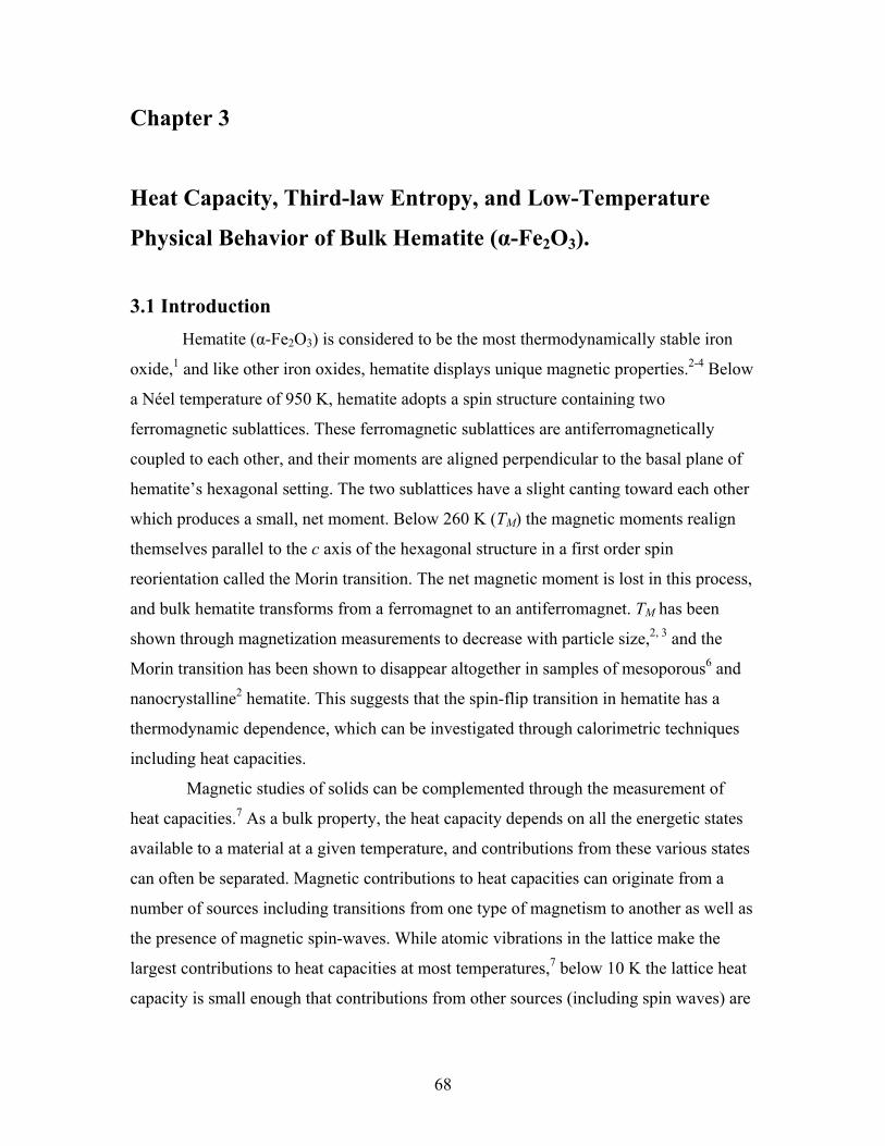
Chapter 3
Heat Capacity, Third-law Entropy, and Low-Temperature
Physical Behavior of Bulk Hematite (α-Fe2O3).
3.1 Introduction Hematite (α-Fe2O3) is considered to be the most thermodynamically stable iron
oxide,1 and like other iron oxides, hematite displays unique magnetic properties.2-4 Below
a Néel temperature of 950 K, hematite adopts a spin structure containing two
ferromagnetic sublattices. These ferromagnetic sublattices are antiferromagnetically
coupled to each other, and their moments are aligned perpendicular to the basal plane of
hematite’s hexagonal setting. The two sublattices have a slight canting toward each other
which produces a small, net moment. Below 260 K (TM) the magnetic moments realign
themselves parallel to the c axis of the hexagonal structure in a first order spin
reorientation called the Morin transition. The net magnetic moment is lost in this process,
and bulk hematite transforms from a ferromagnet to an antiferromagnet. TM has been
shown through magnetization measurements to decrease with particle size,2, 3 and the
Morin transition has been shown to disappear altogether in samples of mesoporous6 and
nanocrystalline2 hematite. This suggests that the spin-flip transition in hematite has a
thermodynamic dependence, which can be investigated through calorimetric techniques
including heat capacities.
Magnetic studies of solids can be complemented through the measurement of
heat capacities.7 As a bulk property, the heat capacity depends on all the energetic states
available to a material at a given temperature, and contributions from these various states
can often be separated. Magnetic contributions to heat capacities can originate from a
number of sources including transitions from one type of magnetism to another as well as
the presence of magnetic spin-waves. While atomic vibrations in the lattice make the
largest contributions to heat capacities at most temperatures,7 below 10 K the lattice heat
capacity is small enough that contributions from other sources (including spin waves) are
68

more easily discerned. Hence, the measurement of heat capacities below 10 K becomes
important in the study of magnetic materials.
Heat capacities can also be used to generate third-law entropies that, when
combined with thermochemical measurements, yield relative free energies of
compounds.8 In turn, free energies give information about the phase stabilities of
materials relative to each other.
The heat capacity of bulk hematite was first measured by Parks and Kelley9 in
1926 over four narrow regions from 90 K to 290 K. In 1958, Westrum and Gronvold5
improved upon these measurements covering the range 5 K to 350 K. No anomaly in the
heat capacity due to the Morin transition was observed in this study or in another later
series of measurements in 1985 by Jayasuriya et al.10 While Jayasuriya did not provide
any values for the entropy of hematite, Westrum and Gronvold5 calculated the entropy of
hematite at 298.15 K to be 87.400 J.mol-1.K-1.
Although heat capacity measurements for hematite exist as low as 5 K, there are
only a few points which makes it difficult to accurately model this data using theoretical
fits. To characterize the magnetic behavior of hematite through heat capacity, it is
necessary to obtain measurements at lower temperatures and with a greater density of
points. This data can be used to investigate spin wave contributions which can provide
details on the magnetic coupling in bulk hematite at low temperatures. The spin wave
contributions can then help determine the extent of the Morin transition and the change to
an antiferromagnet at low-temperatures.
With the goal of studying magnetic coupling in hematite, we report the heat
capacity of hematite in the range 2-300 K measured using a Quantum Design physical
properties measurement system (PPMS). This data was fit to theoretical functions below
10 K, and the results of these fits are discussed. Third law entropies were also calculated
and a comparison is made with previously calculated values.
3.2 Experimental A 1 g sample of nanocrystalline hematite prepared using the method of Liu et al.11
was sintered at 1200oC for 48 hours in an alumina dish. The powder was then slowly
cooled to 500oC at a rate of 10o/min before removing it from the furnace. The XRD
69

spectrum for this sample is shown in Figure 3.1 over the range 25-75o. The peaks are
narrow indicating large crystal size, and the sample is characterized as bulk. Brunauer
Emmet Teller (BET) surface area measurements for this sample also confirm that
sintering the sample has resulted in grain growth with the change in surface area going
from 59.03 m2/g for the nanopowder to 0.0187 m2/g. The chemical purity of this sample
was analyzed using a Perkin-Elmer inductively coupled plasma optical emission
spectrometer (ICP-OES) Optima 4300 DV. A sample solution for ICP was prepared by
dissolving two samples (129.0 and 168.6 mg) of the hematite powder in 50.0 mL of 5%
HNO3. Qualitative analysis of this sample revealed the presence of Al, Ca, Cr, Mn, and
Mg. Quantitative analysis using standard concentrations of these species showed the total
impurities to be less than 0.082 % of the sample mass making the sample 99.918 % pure
on a metals basis.
Figure 3.1. Powder X-ray diffraction spectrum of sintered hematite powder.
70

We have developed new methods of measuring the heat capacity of powdered
samples using the Quantum Design Physical Properties measurement system (PPMS)
with an accuracy of ± 1% from 22 K to 300 K and ± (2-5) % below 22 K, and this
accuracy corresponds to both conducting and non-conducting samples. Details of this
method will be published elsewhere. In general, sample mounting consists of combining
the sample with Apiezon N grease in a copper cup which is then compressed into a pellet
using a stainless steel die. The copper cup is formed from a foil of 0.025 mm thickness
and 99.999 % purity while the pellet has a 2.8 mm diameter and height of 3.5 mm. The
heat capacity of the grease, copper, and addenda are measured as a background which can
be subtracted from measurements including the sample. The heat capacity of the sintered
hematite was measured for two samples (33.25 and 28.57 mg) in the range 2 to 350 K
using the PPMS.
3.3 Results Heat capacity measurements for the two samples are given separately (Tables 2.1
and 2.2) with the 33.25 mg sample referred to as Series 1 and the 28.57 mg sample as
Series 2. This data can be seen graphically with a comparison to that of Westrum and
Gronvold in Figure 2.2, and an inset on this figure shows these graphs below 10 K. The
relative accuracy of the PPMS measurements can be seen by their deviation from the
measurements of Westrum and Gronvold5 in Figure 2.3.
As with the measurements published by Jayasuriya et al10. as well as those by
Westrum and Gronvold,5 no anomaly is observed in the heat capacity measured using
PPMS. Above 30 K the PPMS measurements are within ±0.8% (dashed reference lines in
Figure 3) while below this temperature the data show much larger deviations. There are
two reasons for the large deviations at lower temperatures. First, the heat capacity at low
temperatures is small, and consequently even small deviations will be a much larger
percent of the heat capacity. The second reason for the larger deviations in the heat
capacity comes from the greater degree of error for the measurements by Westrum (5%)
and the PPMS (2%) at temperatures lower than 10 K.
71

Figure 3.2. The heat capacity of hematite measured using PPMS with a comparison to measurements by Westrum and Gronvold.5
Figure 3.3. Percent deviation of the heat capacity measured by PPMS from measurements by Westrum and Gronvold.5
72

Table 3.1. Molar heat capacity of hematite (α-Fe2O3) Series 1. M = 159.69 g·mol-1
T / K Cp,m / (J • K-1 • mol-1) T / K Cp,m / (J • K-1 • mol-1) 1.9541 0.00070104 26.594 1.0593 2.1567 0.00093836 29.495 1.5099 2.3181 0.00115 32.823 2.1561 2.5461 0.0014856 36.516 3.032 2.8188 0.0019405 40.597 4.1877 3.1219 0.0025902 45.138 5.6233 3.4585 0.003456 50.197 7.4647 3.8503 0.0045692 55.788 9.7205 4.2841 0.006133 62.034 12.463 4.755 0.0080633 68.977 15.665 5.2823 0.01059 76.67 19.414 5.8708 0.01379 85.232 23.87 6.5297 0.018178 94.744 28.898 7.2662 0.023863 105.29 34.294 8.0867 0.030711 117.04 40.288 9.0149 0.040392 130.07 46.896 10.176 0.054913 144.59 53.709 11.395 0.074045 160.65 60.907 12.666 0.099194 178.51 68.285 14.074 0.13228 198.45 75.828 15.676 0.18189 220.54 83.465 17.441 0.25158 245.04 90.728 19.331 0.35724 272.19 97.802 21.478 0.50603 302.42 104.51 23.916 0.73218
73

Table 3.2 Molar heat capacity of hematite (α-Fe2O3) Series 2. M = 159.69 g·mol-1
T / K Cp,m / (J • K-1 • mol-1) T / K Cp,m / (J • K-1 • mol-1) 1.9042 0.00076921 26.548 1.0469 2.0321 0.00089922 29.519 1.5018 2.2840 0.0012784 32.838 2.1501 2.5220 0.0016728 36.532 3.0214 2.8041 0.0022341 40.610 4.1605 3.1213 0.0030526 45.150 5.6065 3.4652 0.0040369 50.199 7.4583 3.8467 0.0053558 55.802 9.6894 4.2680 0.0070385 62.039 12.413 4.7556 0.0093363 68.975 15.625 5.3130 0.012390 76.682 19.409 5.8904 0.015619 85.239 23.827 6.5481 0.020407 94.760 28.814 7.2886 0.026202 105.28 34.265 8.1128 0.033507 117.04 40.247 9.0343 0.043294 130.04 46.777 10.224 0.058732 144.57 53.620 11.411 0.077078 160.72 60.834 12.680 0.10093 178.60 68.124 14.088 0.13779 198.53 75.641 15.700 0.18486 220.58 83.282 17.426 0.25149 245.13 90.538 19.324 0.35634 272.48 98.155 21.493 0.50565 302.78 106.92 23.926 0.72611
3.4 Discussion 3.4.1 Contributions to the Heat Capacity of Hematite
Modeling heat capacity data with theoretical functions at low temperatures (< 15
K) can provide valuable information about the magnetic, electronic, and vibrational
properties of a sample.7 The total heat capacity can be viewed as a sum of the energetic
contributions from the various physical properties of a material. At temperatures above
10 K, the largest contribution to heat capacity stems from lattice vibrations which are
modeled by an odd-powers fit to the equation:12
∑=
=...7,5,3n
nnLat TBC . (1)
74

Magnetic contributions will also have a temperature-dependence with 2/3T for ordered
ferro- and ferrimagnets and 3T for antiferromagnets.7
Conduction electrons contribute to the heat capacity in a linear fashion with γT
representing the electronic heat capacity in most cases.7 In addition to conducting solids,
a linear term is generally observed in many oxide materials that are not fully
stoichiometric or which contain oxygen vacancies or dislocations.13 For example, non-
conducting oxides requiring a linear term include α-FeOOH (goethite),13 crystalline pure
SiO2 zeolites,14 and hydrous potassium aluminosilicate15 (muscovite) where the linear
term has been attributed by Coey et al.15 to localized electronic states associated with
oxygen vacancies.
3.4.2 Fits of Bulk Hematite
As seen in the characterization of this sample by XRD, bulk hematite is an
ordered solid which will have a significant lattice contribution of the form
. Magnetic characterization of bulk hematite generally shows that below
the Morin transition hematite is an antiferromagnet which is represented with a
∑= nnLat TBC
3T term.
However in some conditions samples of hematite have shown ferromagnetic behavior at
temperatures as low as 2 K, and consequently some fits were made using a 2/3T term. As
other oxide samples have included a linear term, fits were also made using γT to check
whether the linear term made a significant improvement in representing the heat capacity
of bulk hematite.
The heat capacity of bulk hematite in the temperature range 2 to 10 K was fit with
a wide variety of fitting expressions which consisted of different combinations of the
above terms. A summary of a number of different fits are given in Table 3.3 for bulk
hematite which follow the expression: 2/3
7,5,3TBTBTC fsw
n
nn ++= ∑
=
γ . (2)
Equation 2 can be viewed as a generalized formula that is modified by setting any
coefficient equal to zero. In cases where a coefficient is zero, its corresponding term will
be omitted from the equation.
75

Figure 3.4. Low-temperature fit of bulk hematite heat capacity. Circles are experimental data. Red line is the fit.
Table 3.3. Parameters for equation 3. Units are in mJ, mole, and K. Parameter Fit-1 Fit-2 Fit-3 Fit-4 γ 4.5994E-02 -15.446 B3 (α) 0.083190 8.5981E-02 0.38144 9.4175E-02 B5 -5.8426E-04 -6.2920E-04 2.280 -8.7321E-04 B7 2.6530E-06 2.9055E-06 4.6191E-06 Bfsw 0.039629 10.079 RMS% 0.74 0.83 3.34 2.25
Before a discussion can be given of the thermophysical properties of bulk
hematite it is necessary to determine which of the fits described in Table 3.3 is the best.
Upon immediate inspection it can be seen that Fit-3 has a negative value for γ, which is
physically meaningless. However Fit-3 was included in Table 3.3 because it can still
provide some valuable insight, which will be discussed later on. A comparison of the
%RMS values for the remaining fits shows that Fit-4 has a %RMS of 2.25 which
significantly larger value than 0.74 and 0.83 for Fits 1 and 2 respectively. This suggests
that Fit-4 is missing some contribution that can more accurately represent the heat
capacity of bulk hematite. The %RMS values for Fits 1 and 2 are too similar to allow one
to determine which is the best fit, and more information will be necessary.
A graph of these two fits and experimentally measured data can be found in
Figure 3.5 where it can be seen that both fits match the experimental heat capacity well.
76

To facilitate the comparison of the fits, the percent deviation of Fits 1, 2, and 4 from the
experimentally measured heat capacity of hematite are shown in Figure 3.5.
Fit-4 shows a large degree of error compared to Fits 1 and 2, which display a random
deviation about zero. This indicates that a lattice contribution alone is insufficient to
correctly model the heat capacity of hematite. The similar deviations of Fits 1 and 2 as
well as their low %RMS values make it difficult to conclude whether the linear term or
the ferromagnetic spin wave makes the best fit.
Figure 3.5. Percent deviation of fits from the experimentally measured heat capacity of hematite.
It is important to note that Fit-3 included both a linear term and a ferromagnetic
spin wave, yet was physically meaningless. Likewise other fits that used both terms gave
similar results. This suggests that either hematite has ferromagnetic coupling at low
temperatures or there are electronic contributions due to oxygen deficiencies, but not
both. To determine which fit is the best, it is useful to compare more basic fitting
expressions that use similar terms which allows one to see the effects of a given term on
the fit of the heat capacity. When bulk hematite is fit to the expression a 33TBTC += γ
77

%RMS of 8.84 is obtained while a fit to gave a %RMS of 4.26. This
suggests that the heat capacity of hematite has contributions from a ferromagnetic spin
wave and that Fit-1 is more accurate since such a term can model the heat capacity with
approximately half as much error as a linear term. Furthermore the use of a spin wave is
more likely since some samples of hematite have shown ferromagnetic behavior at low
temperatures.
33
2/3 TBTBC fsw +=
Since hematite is an antiferromagnet below TM, the use of a ferromagnetic spin
wave is surprising. Yet as mentioned previously, under certain conditions hematite has
been shown to have ferromagnetic behavior as low as 2 K. A variety of techniques have
been employed in the study of the magnetic properties of hematite including neutron
diffraction,6 magnetometry,2 and Mossbauer spectroscopy.16 These studies have shown
that small particle size and porous samples of hematite do not undergo the spin-flip
transition and retain their ferromagnetic behavior at low temperatures. The bulk sample
used in these studies was prepared by sintering nanocrystalline hematite, which may
suggest a reason for its observed magnetic properties. The sample characterization clearly
shows grain growth, which eliminates the explanation of small particle size. However the
characterization of bulk hematite was not so clear with respect to the porosity of the
sample. BET surface area measurements were unable to provide a pore size, and the low
surface are suggests that the sample is not very porous. The use of a spin wave in the
fitting expression for this bulk hematite sample suggests that there are other conditions in
which bulk hematite does not undergo the spin-flip transition and will have ferromagnetic
properties at low-temperatures. One of these conditions may be that this sample is
polycrystalline, and heat capacity studies of a single crystal of bulk hematite would be
useful.
Although ferromagnetic behavior has been observed in this bulk hematite sample,
hematite has generally been characterized as antiferromagnetic.2, 6 These two types of
magnetism will not be displayed simultaneously, and it is important to determine whether
or not the 3T term has an antiferromagnetic contribution. This can be accomplished by
examining the contributions to the heat capacity from the 3T term which can stem from a
combination of lattice vibrations and antiferromagnetic coupling.7 Generally, the
antiferromagnetic contributions are ten to twenty times larger than the lattice component
78

at low-temperatures.7 This can be seen in a comparison of the low-temperature heat
capacity of antiferromagnetic MnCO3 and nonmagnetic CaCO3.7 These two samples have
a similar lattice contribution but the contribution of 3T in MnCO3 is many times that of
CaCO3. In the case of hematite, other iron oxides make good candidates for such a
comparison. While the heat capacity of many iron oxides has been measured below 10
K,13, 17, 18 the only published study to give an extensive analysis of the low-temperature
heat capacity involved α-FeOOH (goethite).13 Fits of goethite at low temperatures were
able to separate the contributions of lattice vibrations from antiferromagnetic
contributions. These fits give a value of ~ 0.1 for B3 while the antiferromagnetic
parameter Basw has a value of 1.16, which is about ten times larger. The antiferromagnetic
term for goethite was coupled to an anisotropic gap parameter which does not give the
best comparison to antiferromagnetism. However this bulk hematite and goethite do have
similar lattice terms where B3 for hematite is 0.083 and goethite has a value of 0.1. Other
recent low-temperature fits (unpublished) in our lab of ferrimagnetic 13 nm magnetite
gave a value of 0.587 for B3 which is about 6 times as large as that of bulk hematite. The
similarity between the lattice contributions of goethite and the 3T dependence of
hematite suggests that antiferromagnetic coupling does not exist in hematite at low-
temperatures. Also, the large size of B3 for 13 nm magnetite compared to that of bulk
hematite agrees with this conclusion since 13 nm magnetite is ferrimagnetic.
3.4.3 Thermodynamic Functions of Hematite
The standard molar thermodynamic functions, Cp,m, ΔT0H m, ΔT
0S m, and
Φ m=(ΔT0S m−ΔT
0H m/T) scaled by the ideal gas constant R are reported for Series 1
(Table 3.4) and Series 2 (Table 3.5). The values have been generated at smoothed
temperatures by fitting a combination of orthogonal polynomials to the experimental
results for the two series which were merged with the low-temperature fits. The
parameters for these fits as well as their temperature range can be found in Tables 3.6 and
3.7, respectively. The standard molar entropy at 298.15 K was calculated to be 87.32 ± 2
J.mol-1.K-1 for Series 1 and 87.27 ± 2 J.mol-1.K-1 for Series 2, which are in good
agreement with the value of 87.40 ± 0.2 J.mol-1.K-1 (originally 20.889 cal.deg-1.mole-1)
calculated by Westrum and Gronvold.5
79
Table 3.4. Standard thermodynamic functions of Hematite (α-Fe2O3) Series 1 where Φ = ΔS - ΔH/T, M = 159.69 g·mol-1, p° = 100 kPa, and R = 8.3145 J·K-1·mol-1.
RC mp /, RS om
T /0Δ RTH om
T /0Δ Rom /Φ T/K
2.0 9.11E-05 3.66E-05 2.52E-05 1.14E-05 2.5 0.00017 6.46E-05 4.56E-05 1.90E-05 3.0 0.00028 0.0001 7.48E-05 2.98E-05 3.5 0.00043 0.00016 0.00011 4.41E-05 4.0 0.00061 0.00023 0.00016 6.25E-05 4.5 0.00084 0.00031 0.00023 8.54E-05 5.0 0.00111 0.00041 0.0003 0.00011 5.5 0.00142 0.00053 0.00039 0.00015 6.0 0.00177 0.00067 0.00049 0.00018 6.5 0.00216 0.00083 0.0006 0.00023 7.0 0.00259 0.001 0.00073 0.00028 7.5 0.00307 0.0012 0.00087 0.00033 8.0 0.0036 0.00141 0.00102 0.00039 8.5 0.00419 0.00165 0.00119 0.00046 9.0 0.00483 0.00191 0.00137 0.00053 9.5 0.00555 0.00219 0.00157 0.00061 10 0.00633 0.00249 0.00179 0.0007 11 0.00813 0.00318 0.00228 0.00089 12 0.01025 0.00397 0.00286 0.00111 13 0.01275 0.00489 0.00352 0.00137 14 0.0157 0.00594 0.00428 0.00166 15 0.01917 0.00714 0.00515 0.00198 16 0.02327 0.0085 0.00616 0.00234 17 0.02809 0.01005 0.0073 0.00275 18 0.03371 0.01181 0.00861 0.0032 19 0.04024 0.01381 0.0101 0.00371 20 0.04776 0.01606 0.01179 0.00427 25 0.10296 0.03206 0.02398 0.00808 30 0.19245 0.05819 0.04409 0.0141 35 0.31879 0.09687 0.07388 0.023 40 0.48026 0.14961 0.11423 0.03538 45 0.67256 0.21701 0.16533 0.05168
80

Table 3.4 continued RC mp /, RS o
mT /0Δ RTH o
mT /0Δ Ro
m /Φ T/K
50 0.89066 0.29895 0.22676 0.07219 55 1.13 0.39491 0.29784 0.09706 60 1.3867 0.50412 0.37777 0.12635 65 1.6583 0.62575 0.46575 0.16001 70 1.9425 0.75898 0.56102 0.19797 75 2.2377 0.90301 0.6629 0.24011 80 2.5425 1.0571 0.7708 0.28631 85 2.8541 1.2205 0.88417 0.33641 90 3.1688 1.3926 1.0023 0.39027 95 3.4846 1.5724 1.1247 0.44772 100 3.7999 1.7591 1.2506 0.50859 110 4.4236 2.1507 1.5107 0.63992 120 5.0337 2.5618 1.7791 0.78283 130 5.6269 2.9883 2.0523 0.93598 140 6.2012 3.4264 2.3282 1.0982 150 6.7555 3.8732 2.6051 1.2683 160 7.2887 4.3264 2.8812 1.4452 170 7.8 4.7837 3.1557 1.6281 180 8.2883 5.2435 3.4274 1.8162 190 8.7531 5.7043 3.6955 2.0087 200 9.1945 6.1645 3.9595 2.2049 210 9.6127 6.6234 4.2189 2.4045 220 10.009 7.0797 4.4731 2.6067 230 10.384 7.533 4.722 2.811 240 10.74 7.9824 4.9654 3.0171 250 11.077 8.4278 5.2032 3.2246 260 11.398 8.8686 5.4353 3.4333 270 11.702 9.3045 5.6619 3.6427
273.15 11.794 9.4407 5.732 3.7087 280 11.989 9.7353 5.8827 3.8525 290 12.258 10.161 6.098 4.0628
298.15 12.465 10.503 6.2693 4.2342 300 12.509 10.581 6.3077 4.273
81

Table 3.5. Standard thermodynamic functions of Hematite (α-Fe2O3) Series 2 where Φ = ΔS - ΔH/T, M = 159.69 g·mol-1, p° = 100 kPa, and R = 8.3145 J·K-1·mol-1.
RC mp /, RS om
T /0Δ RTH om
T /0Δ Rom /Φ T/K
2.0 1.05E-04 3.92E-05 5.59E-05 1.12E-05 2.5 1.97E-04 7.18E-05 1.30E-04 1.99E-05 3.0 3.27E-04 1.19E-04 2.59E-04 3.22E-05 3.5 4.99E-04 1.81E-04 4.64E-04 4.88E-05 4.0 7.14E-04 2.61E-04 7.65E-04 7.02E-05 4.5 9.72E-04 3.60E-04 1.18E-03 9.68E-05 5.0 1.27E-03 4.78E-04 1.74E-03 1.29E-04 5.5 1.61E-03 6.14E-04 2.46E-03 1.67E-04 6.0 1.99E-03 7.71E-04 3.36E-03 2.10E-04 6.5 2.41E-03 9.46E-04 4.46E-03 2.60E-04 7.0 2.86E-03 1.14E-03 5.78E-03 3.16E-04 7.5 3.36E-03 1.36E-03 7.33E-03 3.78E-04 8.0 3.90E-03 1.59E-03 9.14E-03 4.46E-04 8.5 4.50E-03 1.84E-03 1.12E-02 5.21E-04 9.0 5.16E-03 2.12E-03 1.37E-02 6.02E-04 9.5 5.88E-03 2.42E-03 1.64E-02 6.89E-04 10 6.67E-03 2.74E-03 1.95E-02 7.84E-04 11 8.46E-03 3.46E-03 2.71E-02 9.93E-04 12 1.06E-02 4.28E-03 3.66E-02 1.23E-03 13 1.31E-02 5.22E-03 4.84E-02 1.50E-03 14 1.60E-02 6.30E-03 6.29E-02 1.81E-03 15 1.95E-02 7.52E-03 8.06E-02 2.14E-03 16 2.36E-02 8.91E-03 1.02E-01 2.52E-03 17 2.83E-02 1.05E-02 1.28E-01 2.94E-03 18 3.39E-02 1.22E-02 1.59E-01 3.41E-03 19 4.03E-02 1.42E-02 1.96E-01 3.93E-03 20 4.76E-02 1.65E-02 2.40E-01 4.50E-03 25 1.02E-01 3.24E-02 6.01E-01 8.34E-03 30 1.91E-01 5.83E-02 1.32E+00 1.44E-02 35 3.17E-01 9.68E-02 2.58E+00 2.32E-02 40 4.78E-01 1.49E-01 4.55E+00 3.55E-02 45 6.69E-01 2.16E-01 7.41E+00 5.18E-02
82

Table 3.5 continued RC mp /, RS o
mT /0Δ RTH o
mT /0Δ Ro
m /Φ T/K
50 8.87E-01 2.98E-01 1.13E+01 7.22E-02 55 1.13E+00 3.94E-01 1.63E+01 9.70E-02 60 1.38E+00 5.02E-01 2.26E+01 1.26E-01 65 1.66E+00 6.24E-01 3.02E+01 1.60E-01 70 1.94E+00 7.57E-01 3.91E+01 1.97E-01 75 2.23E+00 9.00E-01 4.96E+01 2.40E-01 80 2.54E+00 1.05E+00 6.15E+01 2.86E-01 85 2.85E+00 1.22E+00 7.50E+01 3.36E-01 90 3.16E+00 1.39E+00 9.00E+01 3.89E-01 95 3.48E+00 1.57E+00 1.07E+02 4.47E-01 100 3.79E+00 1.76E+00 1.25E+02 5.07E-01 110 4.42E+00 2.15E+00 1.66E+02 6.38E-01 120 5.03E+00 2.56E+00 2.13E+02 7.81E-01 130 5.62E+00 2.98E+00 2.66E+02 9.34E-01 140 6.19E+00 3.42E+00 3.25E+02 1.10E+00 150 6.74E+00 3.87E+00 3.90E+02 1.27E+00 160 7.27E+00 4.32E+00 4.60E+02 1.44E+00 170 7.78E+00 4.77E+00 5.35E+02 1.62E+00 180 8.27E+00 5.23E+00 6.16E+02 1.81E+00 190 8.73E+00 5.69E+00 7.01E+02 2.00E+00 200 9.17E+00 6.15E+00 7.90E+02 2.20E+00 210 9.59E+00 6.61E+00 8.84E+02 2.40E+00 220 9.98E+00 7.06E+00 9.82E+02 2.60E+00 230 1.04E+01 7.52E+00 1.08E+03 2.81E+00 240 1.07E+01 7.96E+00 1.19E+03 3.01E+00 250 1.11E+01 8.41E+00 1.30E+03 3.22E+00 260 1.14E+01 8.85E+00 1.41E+03 3.43E+00 270 1.17E+01 9.29E+00 1.53E+03 3.63E+00
273.15 1.18E+01 9.42E+00 1.56E+03 3.70E+00 280 1.21E+01 9.72E+00 1.64E+03 3.84E+00 290 1.24E+01 1.01E+01 1.77E+03 4.05E+00
298.15 1.27E+01 1.05E+01 1.87E+03 4.23E+00 300 1.28E+01 1.06E+01 1.89E+03 4.26E+00
83

Table 3.6. Parameters for fits of the heat capacity of hematite Series 1. Units are in J, mole, and K.
Powers Temperature Ranges Coefficients 0 ≤ T (K) ≤ 9.9
1 3.620950E-05 3 8.870109E-05 5 -7.995470E-07 7 6.075500E-09 9 -1.718381E-11
9.9 ≤ T (K) ≤ 76.0 0 1.584123E-01 1 -6.904413E-02 2 1.225543E-02 3 -1.034390E-03 4 5.035171E-05 5 -1.270369E-06 6 1.855010E-08 7 -1.597010E-10 8 7.566424E-13 9 -1.527721E-15
76.0 ≤ T (K) ≤ 305.0 0 4.333282E+01 1 -2.573582E+00 2 6.278703E-02 3 -7.023903E-04 4 4.793339E-06 5 -2.057930E-08 6 5.401251E-11 7 -7.903096E-14 8 4.933786E-17
84
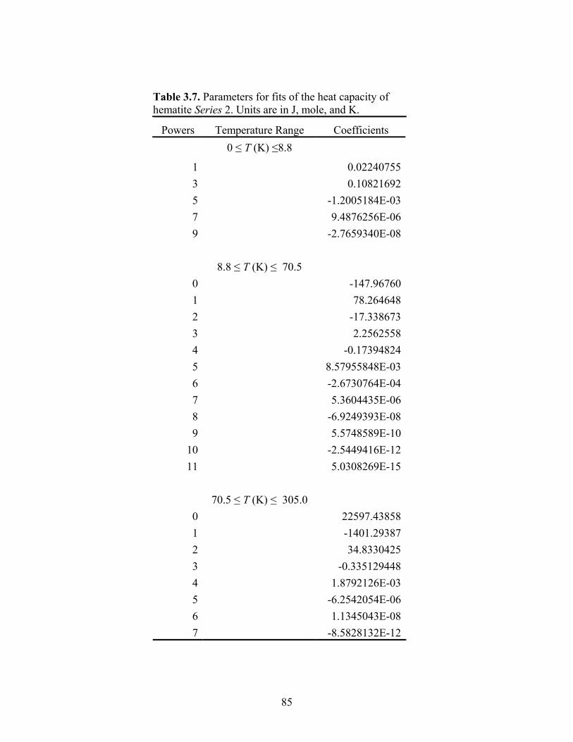
Table 3.7. Parameters for fits of the heat capacity of hematite Series 2. Units are in J, mole, and K.
Powers Temperature Range Coefficients 0 ≤ T (K) ≤8.8
1 0.022407553 0.108216925 -1.2005184E-037 9.4876256E-069 -2.7659340E-08
8.8 ≤ T (K) ≤ 70.5
0 -147.967601 78.2646482 -17.3386733 2.25625584 -0.173948245 8.57955848E-036 -2.6730764E-047 5.3604435E-068 -6.9249393E-089 5.5748589E-10
10 -2.5449416E-1211 5.0308269E-15
70.5 ≤ T (K) ≤ 305.0
0 22597.438581 -1401.293872 34.83304253 -0.3351294484 1.8792126E-035 -6.2542054E-066 1.1345043E-087 -8.5828132E-12
85
References
1. Cornell, R. M.; Schwertmann, U.; Editors, The Iron Oxides: Structure, Properties, Reactions, Occurrence and Uses. VCH: Weinem, 1996; p 573.
2. Bahl, C. R. H. The magnetic properties of antiferromagnetic nanoparticles: NiO and alpha -Fe2O3; Information Service Department,Riso National Laboratory,Roskilde,Den.: 2006; pp i-vi,1-100.
3. Carbone, C.; Di Benedetto, F.; Sangregorio, C.; Marescotti, P.; Pardi, L. A.; Sorace, L., J. Phys. Chem. C 2008, 112 (27), 9988-9995.
4. Lee, J. D., Phys. Rev. B: Condens. Matter Mater. Phys. 2004, 70 (17), 174450/1-174450/6.
5. Gronvold, F.; Westrum, E. F., Jr., J. Am. Chem. Soc. 1959, 81, 1780-3. 6. Hill, A. H.; Jiao, F.; Bruce, P. G.; Harrison, A.; Kockelmann, W.; Ritter, C.,
Chem. Mater. 2008, 20 (15), 4891-4899. 7. Gopal, E. S. R., Specific Heats at Low Temperatures (International Cryogenics
Monograph Series). Plenum Press: New York, 1966; p 226 8. Ott, J. B.; Boerio-Goates, J., Chemical Thermodynamics: Principles and
Applications. 2000; p 360 pp. 9. Parks, G. S.; Kelley, K. K., J. Phys. Chem. 1926, 30, 47-55. 10. Jayasuriya, K. D.; Stewart, A. M.; Campbell, S. J., J. Phys. Chem. Solids 1985, 46
(5), 625-9. 11. Liu, S.; Liu, Q.; Boerio-Goates, J.; Woodfield, B. F., J. Adv. Mater. (Covina, CA,
U. S.) 2007, 39 (2), 18-23. 12. Phillips, N. E., Crit. Rev. Solid State Sci. 1971, 2 (4), 467-553. 13. Majzlan, J.; Navrotsky, A.; Woodfield, B. F.; Lang, B. E.; Boerio-Goates, J.;
Fisher, R. A., J. Low Temp. Phys. 2003, 130 (1/2), 69-76. 14. Boerio-Goates, J.; Stevens, R.; Lang, B.; Woodfield, B. F., J. Therm. Anal.
Calorim. 2002, 69 (3), 773-783. 15. Coey, J. M. D.; Von Molnar, S.; Torressen, A., J. Less-Common Met. 1989, 151,
191-4. 16. Morup, S.; Frandsen, C.; Bodker, F.; Klausen, S. N.; Lefmann, K.; Lindgard, P.-
A.; Hansen, M. F., Hyperfine Interact. 2003, 144/145 (1-4/1-4), 347-357. 17. Majzlan, J.; Lang, B. E.; Stevens, R.; Navrotsky, A.; Woodfield, B. F.; Boerio-
Goates, J., Am. Mineral. 2003, 88 (5-6), 846-854. 18. Koenitzer, J. W.; Keesom, P. H.; Honig, J. M., Phys. Rev. B: Condens. Matter
Mater. Phys. 1989, 39 (9), 6231-3.
86

87
Chapter 4
Size-Dependence of the Heat Capacity and Thermodynamic
Properties of Hematite (α-Fe2O3)
4.1 Introduction
Hematite (α-Fe2O3) is considered to be the most stable form of iron oxide, and
can be found naturally in rocks, mud, and water systems.2, 3
The catalytic, electronic, and
magnetic properties of hematite have been extensively investigated leading to a wide
variety of applications. Some technologies that employ hematite include gas sensors,
electrode materials in lithium secondary batteries, catalysts, magnetic recording media,
and optical and electromagnetic devices as well as water splitting treatments.3-7
In
addition to its many applications, the use of hematite is attractive owing to its
nontoxicity, low processing cost, and high resistance to oxidative change.7, 8
Studies involving hematite have begun to focus on the size-dependence of its
chemical and physical properties, and a comparison of bulk and nanoscale behavior
reveals significant changes in the properties of hematite. Some studies9, 10
have
concluded that small particle size may alter the energy positions of the electronic states
that define the semiconductor band gap, yet a recent study suggests no change in the
electronic properties of hematite.11
The magnetic behavior of nanocrystalline hematite
has also been shown to deviate from that of bulk hematite.12-26
At room temperature bulk
hematite is weakly ferromagnetic, but below 260 K (TM) hematite undergoes a first order
spin reorientation called the Morin transition. The net magnetic moment is lost in this
process, and bulk hematite transforms into an antiferromagnet. In contrast, magnetization
studies on nanocrystalline and mesoporous samples of hematite show that no spin
reorientation occurs upon cooling, and ferromagnetic behavior persists as low as 2 K.7
Many studies also show that hematite nanoparticles display superparamagnetic
properties.8-10

88
In addition to magnetic and electronic measurements, thermodynamic studies of
nanosystems provide sophisticated characterization and a more quantitative approach to
phase stability. A comprehensive thermodynamic study of the many iron oxides and iron
oxyhyrdoxides (FeOOH) has been undertaken by Navrotsky and coworkers11-19
who have
recently published a summary of current thermodynamic understanding of these
materials.11
This work has included the measurement of heat capacities and
thermochemical measurements which can be used to obtain the standard Gibbs free
energy of formation at 298.15 K, and bulk hematite has been shown to be the most stable
iron oxide with a Gibbs free energy of formation of -744.4 ± 1.3 kJ/mol. In these studies,
the importance of particle size and degree of hydration has been a key point in
determining the energetics of the iron oxide polymorphs.11
Surface enthalpy (whether
comparing wet or dry surfaces) has been shown to be much higher for the anhydrous
phases (oxides) than for any of the hydrous phases (oxyhyrdoxides). A lower surface
enthalpy allows oxyhydroxides to exist with larger surface areas and to be
thermodynamically more competitive at smaller particle sizes.11
This can be seen in the
dehydration reaction from goethite (α-FeOOH) to hematite (2FeOOH = Fe2O3 + H2O)
where smaller particle sizes allow goethite to persist to temperatures more than 100 K
higher than those calculated by bulk thermodynamic relationships.11
Another observation
of surface enthalpy measurements is that materials with the highest surface enthalpy are
stabilized by the adsorption of water.11
As metastability of the bulk phase increases its
surface enthalpy decreases, which has been seen as possibly a close to universal trend and
not just with the iron oxides.20
The decrease of surface enthalpy with increasing
metastability of the bulk polymorphs leads to crossovers in free energy of the polymorphs
at the nanoscale.11
This has been seen in the iron oxides as γ-Fe2O3 (maghemite) becomes
stable with respect to hematite at the nanoscale, and there are complex crossovers for the
FeOOH polymorphs as well.11
This phenomenon emphasizes the need to consider
nanoscale phenomena when studying phase stability and reactivity. In general, the
thermodynamics of different polymorphs at the nanoscale depends on the energetics of
the bulk polymorphs, the particle size, and the extent of hydration.11
Size driven thermodynamic differences among iron oxide phases must be taken
into account if the formation, stability, and transformation of these materials in geologic,

89
environmental, and industrial settings are to be understood and predicted.11
Heat capacity
measurements of nanocrystalline hematite can aid in this understanding as they can
provide information about the density of vibrational states as well as the electronic and
magnetic properties of solids.27, 30
Heat capacities can also be used to generate third-law
entropies that, when combined with thermochemical measurements, yield relative free
energies of the nanoparticles. In turn, free energies give information about the phase
stabilities of the particles relative to each other and to their parent bulk materials.
The heat capacity of bulk hematite was first measured by Parks and Kelley in
1926 over four narrow regions from 90 K to 290 K.27, 28, 31
In 1958, Westrum and
Gronvold improved upon these measurements covering the range from 5 K to 350 K.6 No
anomaly in the heat capacity due to the Morin transition was observed in this study or in
another later series of measurements in 1985 by Jayasuriya et al.21
While Jayasuriya did
not provide any values for the entropy of hematite, Westrum and Gronvold calculated the
entropy of hematite at 298.15 K to be 87.40 J.mol
-1.K
-1. Recently, the heat capacity of
nanocrystalline hematite was measured in the temperature range 253 to 283 K with a
reported accuracy of ± 1.5%.22
Because of its small temperature range, this data is
insufficient to calculate the entropy associated with nanocrystalline hematite; however,
the authors state that their research purpose was to study the magnetocaloric effect in
nanosystems, and thus thermodynamic calculations and physical modeling of heat
capacity were not within their scope.
While the heat capacity of nanocrystalline hematite has not been adequately
measured, heat capacity measurements for several metal and metal oxide nanoparticle
systems are available.27, 34-39
It was previously accepted that the heat capacity of
nanoparticles exceeds that of their bulk counterparts with the larger heat capacity being
attributed to the increase of surface atoms, which have different vibrational modes than
interior atoms.23, 24, 25
More recently, a careful study regarding the origin of the excess
heat capacity in nanoparticles was carried out by Boerio-Goates et al.4 on anatase and
rutile polymorphs of TiO2. The heat capacity of 7 nm TiO2 nanoparticles decreased
proportionally with the degree of hydration, and the excess heat capacity was shown to be
caused by water adsorbed onto the surface of the nanoparticles. When the contributions
of the adsorbed water were subtracted from the heat capacity it was shown that, within

90
experimental error, the bare small particle heat capacity was the same as that of the bulk.
Also, the water showed two types of behavior. Layers of water closer to the surface of the
nanoparticles had a low heat capacity due to tight binding while outer layers were similar
to liquid water. These studies by Boerio-Goates et al. agree with the conclusions of
Navrotsky et al.11
that the degree of hydration must be taken into account when studying
the thermodynamic properties of nanosystems.
This work aims to complement the thermodynamic studies of the iron oxides
undertaken by Navrotsky et al. Like the measurements carried out on nanocrystalline
TiO2 polymorphs4 this study will compare the thermodynamic properties of
nanocrystalline hematite to those of the bulk material. This study provides the heat
capacity of a hematite powder with an average crystal size of 13 nm in the temperature
range 1.5 to 350 K. A comparison to new bulk hematite data measured from 2 to 300 K
(to be published separately) is made with a discussion on the effects of water adsorbed
onto the surface of nanocrystalline hematite.
4.2 Experimental
Nanocrystalline hematite was prepared through a solid state reaction following the
method described by Liu et al.26
Solid NH4HCO3 was combined with 99.99% pure
Fe(NO3)3.9H2O in a 3:1 Fe
3+:HCO3
- molar ratio. The mixture of the two dry powders
turned into a wet slurry which rapidly produced bubbles of CO2(g). The mixture was
continuously ground (15-30 minutes) in an alumina mortar until the evolution of bubbles
ceased. A dark brown solid precipitated in this slurry which was dried in air at 50oC for
20 hours. The solid powder was then rinsed with water using a vacuum filtration flask,
transferred to a pyrex dish, then calcined in air at 270oC for 45 minutes.
The sample was characterized by powder x-ray diffraction (XRD) on a Scintag
Diffractometer (Cu-Kα radiation, λ = 1.54176 nm) at a scanning rate of 0.1 2θ/min and a
power of 15 kW over the range 25 to 70o. The resulting pattern (Figure 4.1) showed the
product to be pure hematite in agreement with JCPDS card number 00-001-1053. Using
the full peak width at half the maximum intensity and the Scherrer formula, the average
crystallite diameter was calculated to be 13 nm.

91
A sample was prepared for transmission electron microscopy (TEM) by
dispersing a small amount of hematite powder in ethanol and grinding with an agate
mortar and pestle. The mixture was allowed to rest for 24 hours in a glass test tube
before drawing off the supernatant. A drop of this suspension was then placed on a
copper grid with 3 nm carbon backing and microscopy images were acquired using a
Tecnai F30 TEM. Micrographs of the hematite powder are shown in Figures 4.2a and
4.2b. Figure 4.2a, which show the particles at 200 kx magnification gives an idea of the
size dispersion and morphology. The particles are roughly spherical, and most have a
diameter of ~ 10 nm. Figure 4.2b shows these particles at 310 kx where ordered atomic
planes can be seen, indicating that these particles are highly crystalline in agreement with
the results of XRD.
Figure 4.1. Powder X-ray Diffraction spectrum of hematite powder.

92
Brunauer Emmett Teller (BET) surface area measurements were performed using
a nitrogen adsorption isotherm on a Micromeritics Tristar 3020. The nano-hematite
powder was found to have a surface area of 59.0 m2/g. A spherical particle size
equivalent can be calculated from surface area measurements using the formula:
1000**
6)(
ρSAnmd = ,
where ρ is the density of the sample. Approximating the density of the nanopowder to be
that of bulk hematite (5.25 g/cm3) the particle size is calculated to be 19.4 nm. This
formula assumes the particles to have cubic shape, however if a spherical particle is
assumed then this value can be multiplied by the ratio of the surface area of a sphere to
that of a cube (0.523), which gives a value of 10.1 nm, which is in much better agreement
with the results from XRD and TEM.
Anlaysis of chemical impurities was performed using a Perkin-Elmer inductively
coupled plasma optical emission spectrometer (ICP-OES) Optima 4300 DV. A sample
solution for ICP was prepared by dissolving two samples (129.0 and 168.6 mg) of the
hematite powder in 50.0 mL of 5% HNO3. Qualitative analysis of this sample revealed
the presence of Al, Ca, Cr, Mn, and Mg. Quantitative analysis using standard
concentrations of these species showed the total impurities to be less than 0.082% of the
Figure 4.2b. Transmission electron
micrograph of hematite nanoparticles
At 310 kx magnification
Figure 4.2a. Transmission electron
micrograph of hematite nanoparticles
At 200 kx magnification

93
sample mass making the sample 99.918% pure on a metals basis. An analysis of carbon,
nitrogen, and hydrogen by combustion at Galbraith Laboratories showed the nitrogen
residue from the NH4HCO3 to be 68 ppm while the carbon and hydrogen contents were
less than 0.5%.
Thermal gravimetric analysis (TGA) of the sample was carried out in corundum
crucibles using a Netzsch 409 system. The sample was heated at a rate of 8.0oC/min to
1000oC in He(g) resulting in a 2.80% mass loss. Assuming all the mass lost to be water,
this equates to a percent mass of hydrogen of 0.313%, which agrees well with the
Galbraith results of less than 0.5%. With a detailed characterization the chemical formula
of the hematite nanopowder used in this study is represented as Fe2O3.0.248H2O with a
molecular weight of 164.156 g/mol.
The sample was prepared for adiabatic calorimetry by compressing the powder
into pellets of 3/8” diameter which were then broken and placed in the calorimetric vessel
described by Stevens and Boerio-Goates.27
This container was evacuated and refilled
with 0.080 mmoles of dry He(g). The calorimeter was then sealed by pressing a 0.7620 g
gold gasket against a stainless steel knife edge located at the top of the vessel. Heat
capacity measurements were made on this system over the temperature range 30 to 350
K.
The heat capacity of this sample was also measured in the temperature range 0.5
to 38 K using the semi-adiabatic calorimeter described by Lashley et al.28
This was done
using a 0.1906 g sample wrapped in a 0.0841 g copper foil (99.999% pure) to provide
greater thermal conductivity. The copper and hematite nanopowder were compressed into
a pellet of 3/8” diameter and 1/8” thickness which was then attached to the sample
platform of the apparatus by using Apiezon N grease. The contributions of the copper,
grease, and addenda were subtracted to obtain the molar heat capacity of nanocrystalline
hematite.
4.3 Results
Experimental results for the molar heat capacity mpC , of the nanocrystalline
hematite powder are given in Table 4.1 along with the temperature increments ∆T for
each heat capacity measurement. Figure 4.3 shows the results graphically with a

94
comparison to two bulk data sets measured by PPMS as well as the heat capacity of bulk
hematite measured by Westrum and Gronvold.6 The heat capacity divided by temperature
is shown in the temperature range 1.5 to10 K in Figure 4.4.
It can be seen in these graphs that, like other nanomaterials, the heat capacity of
nanocrystalline hematite is larger than that of the bulk. Also, the spin-flip transition at TM
is not observed in the heat capacity of nanocrystalline hematite. However, no anomaly
was observed in the heat capacity of bulk hematite as well.6, 21
Another feature in this
data is seen in the region from 4 to 7 K where there is a small, broad anomaly. A
discussion of the physical implications of the features observed in the heat capacity of
nanocrystalline hematite is given below.
The heat capacity was experimentally measured as low as 0.5 K, but an
examination of the data by plotting C/T vs 2T (Figure 4.5) showed an inflection at T =
1.3 K at which point the data began to trend towards negative values. Attempts to fit the
heat capacity of nanocrystalline hematite including these points resulted in large degrees
of error, and it was determined that data below 1.3 K did not achieve thermal equilibrium
Figure 4.3. Heat Capacity of 13 nm hematite compared to the bulk
including measurements by Westrum.6

95
during the measurement process.
Figure 4.4. Heat capacity of 13 nm hematite below 10 K. Temperature is
shown on a log scale. A comparison is made to the bulk including
measurements by Westrum.6
Figure 4.5. A graph of C/T vs T 2 which shows a trend in the data where the heat
capacity begins to drop towards negative values at T 2 = 1.8 (T = 1.3 K).

96
Table 4.1. Experimental heat capacity of nanocrystalline hematite.
M = 164.156 g · mol−1
T/K Cp,m (J mol-1
K-1
) ∆T/K T/K Cp,m (J mol-1
K-1
) ∆T/K
Series 1 40.15 5.396 3.57
159.13 64.866 2.82 43.91 6.769 3.95
163.08 66.801 5.09 Series 11
168.18 69.052 5.09 41.99 5.859 3.43
173.28 71.343 5.10 45.62 7.280 3.75
177.77 73.225 3.88 49.61 8.942 4.24
Series 2 54.08 11.135 4.69
192.39 79.228 5.12 59.05 13.386 5.22
197.50 81.318 5.11 Series 12
202.62 83.259 5.12 1.726 0.002622 0.166
207.75 85.126 5.13 1.897 0.002977 0.185
212.88 86.969 5.13 2.088 0.003394 0.199
218.01 88.857 5.13 2.298 0.003988 0.220
223.14 90.638 5.14 2.528 0.004683 0.240
228.28 92.283 5.14 2.781 0.005564 0.266
Series 3 3.060 0.006745 0.292
219.40 89.20 5.11 3.368 0.008285 0.323
224.52 91.03 5.14 Series 13
229.65 92.74 5.14 9.157 0.09291 0.875
234.79 94.41 5.14 10.073 0.11885 0.964
239.94 96.09 5.14 11.082 0.15264 1.060
245.08 97.63 5.15 12.191 0.19559 1.164
250.23 99.22 5.15 13.404 0.25298 1.270
255.38 100.68 5.15 14.740 0.32877 1.414
260.53 102.23 5.15 16.222 0.41833 1.559
265.68 103.70 5.16 17.845 0.56851 1.705
270.83 105.12 5.16 19.632 0.75521 1.880
275.99 106.43 5.16 21.601 0.99091 2.065
Series 4 23.761 1.33421 2.266
263.07 102.817 5.40 26.119 1.77470 2.464
268.34 104.287 5.15 28.712 2.34062 2.738
273.50 105.659 5.16 31.578 3.10029 3.010
278.66 106.883 5.17 34.730 4.09817 3.311
283.82 108.345 5.15 37.552 4.93222 2.352
288.97 109.750 5.16 Series 14
294.14 111.168 5.17 1.812 0.002819 0.173
299.30 112.446 5.16 1.992 0.003221 0.190
304.46 113.746 5.17 2.193 0.003749 0.207
309.62 115.080 5.17 2.411 0.004362 0.231
314.78 116.255 5.18 2.654 0.004985 0.251
319.95 117.371 5.17 2.923 0.006086 0.280

97
T/K Cp,m (J mol-1
K-1
) ∆T/K T/K Cp,m (J mol-1
K-1
) ∆T/K
Series 5 3.212 0.007206 0.307
296.58 111.778 5.25 3.534 0.009041 0.336
301.78 112.954 5.16 3.887 0.010769 0.366
306.94 114.080 5.17 4.275 0.013272 0.407
312.11 115.455 5.16 4.701 0.017728 0.448
Series 6 5.170 0.022685 0.491
317.23 116.357 5.11 5.684 0.029664 0.543
322.37 117.499 5.17 6.258 0.037346 0.594
327.54 118.725 5.17 6.883 0.046173 0.657
332.71 119.710 5.17 7.570 0.056935 0.717
337.88 120.881 5.17 8.327 0.070361 0.790
343.05 121.706 5.17 9.152 0.091213 0.871
348.23 122.697 5.17 10.066 0.115613 0.962
353.41 123.683 5.17 Series 15
Series 7 9.618 0.1051 0.921
60.08 13.824 9.50 10.580 0.1347 1.005
67.01 17.274 4.35 11.637 0.1732 1.110
71.54 19.555 4.72 12.795 0.2251 1.206
76.28 22.039 4.75 14.068 0.2892 1.342
81.05 24.610 4.79 15.477 0.3777 1.481
85.87 27.239 4.83 17.032 0.4961 1.631
90.72 29.910 4.87 18.741 0.6542 1.792
95.61 32.646 4.90 20.622 0.8588 1.972
100.53 35.339 4.93 22.684 1.1514 2.164
105.47 38.038 4.95 24.942 1.5389 2.367
110.43 40.766 4.97 27.419 2.0477 2.601
115.41 43.479 4.99 30.145 2.6922 2.858
Series 8 33.149 3.5614 3.172
97.87 33.802 4.39 36.140 4.5749 2.842
102.54 36.431 4.95 Series 16
107.49 39.181 4.96 1.347 0.001791 0.127
112.46 41.860 4.98 1.482 0.002085 0.141
117.45 44.531 5.00 1.628 0.002422 0.157
122.46 47.181 5.01 1.792 0.002754 0.175
127.47 49.832 5.02 1.972 0.003172 0.189
132.50 52.410 5.04 2.169 0.003644 0.208
137.55 54.939 5.05 Series 17
142.60 57.439 5.06 1.418 0.001945 0.139
147.66 59.898 5.06 1.558 0.002264 0.143
152.73 62.287 5.08 1.711 0.002560 0.165
Series 9 1.883 0.002921 0.179
157.82 64.487 5.03 2.070 0.003370 0.197

98
4.4 Discussion
4.4.1 The Morin Transition
The absence of an anomaly in the region of the Morin transition is not surprising
since the transition was not observed in the heat capacity of bulk hematite.29, 32
Various
studies have placed the temperature of the Morin transition where the sample changes
from ferromagnetic to antiferromagnetic at 250 K.7, 21
It has been suggested that the heat
capacity shows no sign of transition in this region because either it does not involve any
appreciable entropy increment or that it is spread out over a rather broad temperature
range.6 Although the Morin transition has not shown a significant contribution to the heat
capacity of hematite, low-temperature fits can help determine whether or not a magnetic
transition has occurred. The following discussion is an analysis of the physical properties
of 13 nm hematite that are extracted from low-temperature theoretical fits.
4.4.2 Thermophysical Properties of Nanocrystalline Hematite
Modeling heat capacity data with theoretical functions at low temperatures (< 15
K) can provide valuable information about the magnetic, electronic, and vibrational
properties of a sample.29
The total heat capacity can be viewed as a sum of the energetic
contributions from the various physical properties of a material. At temperatures above
10 K, the largest contribution to heat capacity stems from lattice vibrations which are
modeled by an odd-powers fit to the equation:
T/K Cp,m (J mol-1
K-1
) ∆T/K T/K Cp,m (J mol-1
K-1
) ∆T/K
162.88 66.732 5.09 Series 18
167.97 69.077 5.09 3.700 0.009972 0.362
173.07 71.383 5.10 4.075 0.012323 0.386
178.17 73.645 5.11 4.480 0.015204 0.427
183.28 75.730 5.11 4.928 0.019739 0.468
188.39 77.781 5.12 5.419 0.025729 0.517
193.51 79.806 5.12 5.960 0.032922 0.566
198.63 81.777 5.12 6.556 0.041086 0.626
203.75 83.657 5.13 7.211 0.051480 0.683
208.88 85.606 5.13 7.928 0.063731 0.755
214.01 87.424 5.13 8.721 0.081892 0.834
Series 10 9.592 0.10372 0.917
31.01 2.566 2.41 10.552 0.13197 1.010
36.77 4.261 3.19

99
∑=
=...7,5,3n
n
nLat TBC .30
(1)
Magnetic contributions will also have a temperature-dependence with 2/3T for ordered
ferro- and ferrimagnets and 3T for antiferromagnets. If there is a significant amount of
anisotropy the spin-wave spectrum will have a gap,45, 46
which is similar to the gap
induced by a magnetic field. Gaps in magnetic solids require the use of the term
T
fswfsw eTBC/2/3 ∆−= for ferro- and ferrimagnets and T
aswasw eTBC/3 ∆−= for
antiferromagnets, where ∆ is the gap parameter given in units of K. Fits are made by
combining some of these models, and a physically meaningful expression that represents
the heat capacity of nanocrystalline hematite can be obtained.
Conduction electrons contribute to the heat capacity in a linear fashion with γT
representing the electronic heat capacity in most cases.29
In addition to conducting solids,
a linear term is generally observed in many oxide materials that are not fully
stoichiometric or which contain oxygen vacancies or dislocations.29
For example, non-
conducting oxides requiring a linear term include α-FeOOH (goethite),1 crystalline pure
SiO2 zeolites,31
and hydrous potassium aluminosilicate32
(muscovite) where the linear
term has been attributed by Coey et al.31
to localized electronic states associated with
oxygen vacancies.
Superparamagnetic effects33, 34
can also contribute to the heat capacity.
Superparamagnetism occurs in nanoparticles that consist of a single magnetic domain
with a diameter between 3 and 50 nm. Unlike the effects of paramagnetism which are
usually observed above the Curie temperature, superparamagnetism occurs below this
point. This magnetic behavior is characterized by the entire nanoparticle acting as a
single magnetic moment which can randomly flip direction under the influence of
temperature. Superparamagnetism can be manifest as a dipolar contribution to the heat
capacity due to the interaction of each spin cluster with the dipolar field created by all the
other neighbors. 35, 36
This dipolar field depends on the spin configuration of the
neighboring spins, which is dependent on the overall magnetization, and in the absence of
a magnetic field the probability distribution of the internal fields is centered at zero. The
heat capacity of ideal superparamagnets frequently exhibits an upturn in the heat capacity
at temperatures lower than 1 K as shown in reports by Triplett and Phillips.33
Livingston

100
and Bean34
proposed that superparamagnetic effects might make a measurable
contribution to γ under optimal conditions which include small particle size and positive
anisotropy energy. This model is limited by its neglect of interactions between particles,
yet a linear term has been observed in other superparamagnetic systems.33
4.4.3 Fits of the Heat Capacity of 13 nm Hematite
The presence of a small anomaly in the heat capacity ranging from 4 to 7 K
presented some difficulties in modeling the thermophysical behavior of nanocrystalline
hematite. Attempts to model this data with a Schottky (2-level system) or a magnetic spin
gap produced physically meaningless results with parameters having negative values. The
points in the region of the anomaly were omitted in subsequent fits, which were done in
the range 1.4 to 15 K. This approach was successful, and the heat capacity of
nanocrystalline hematite is expressed as:
5
5
3
3, TBTBTC mp ++= γ (2).
Table 4.2 contains the parameters for this expression (Fit-1) as well as those for
other fits of the heat capacity of nanocrystalline hematite. An inspection of this table
shows that Fits 2 and 3 do not accurately represent the heat capacity of 13 nm hematite as
seen by their high %RMS values. Fits 1 and 4 have a similar %RMS, but Fit-4 has a
small negative value for Bfsw. A negative parameter is physically meaningless, but this
value is small enough that the spin-wave contribution be approximated to be zero.
Consequently, Fit-4 has the same expression as that of Fit-1, which suggests that Fit-1
gives the most accurate representation of the heat capacity of 13 nm hematite. Support for
this conclusion can also be seen in the deviation of the various fits (Figure 4.6) which
shows that only Fit-1 has a random distribution about zero in the given temperature
range. Also, the low-temperature heat capacity of nanocrystalline hematite is compared
with Fit-1 in Figure 4.7 where it can be seen that this fit agrees well with experimental
measurements except in the region of the anomaly from 4 to 8 K.

101
4.4.4 Physical Meaning of Fit-1
Fit-1 included terms for the lattice heat capacity and a linear contribution, but no
ferromagnetic spin wave. This is surprising since several studies indicated that
nanocrystalline hematite did not undergo the spin-flip transition to antiferromagnetic
behavior, but that it retained ferromagnetic behavior as low as 2 K.7, 9, 37-41
One possible
explanation for this observation is that the sample has transformed to antiferromagnetic
which would be manifest in the use of a T 3 term. A second explanation is that the
ferromagnetic spin wave contribution is so small that it does not make a significant
difference in the fitting expression, yet this is unlikely since Fits 2 and 3 show that Bfsw
can be large but not accurately represent the heat capacity data. Another possibility is that
13 nm hematite does not order magnetically at low temperatures. An analysis of the T 3
Table 4.2. A summary of fits of low-temperature heat capacity of 13
nm hematite. Units are in mJ, mole, and K.
Parameter Fit-1 Fit-2 Fit-3 Fit-4
B3 0.098187 0.087202 0.070020 0.10080
B5 -5.9318E-05 4.3157E-05 -6.9112E-05
γ 1.0235 0.82085 1.1129
Bfsw 0.17695 0.79806 -0.070675
%RMS 1.47 2.35 4.84 1.42
Figure 4.6. Deviation of Fits 1-3 from the low-temperature experimental
heat capacity of 13 nm hematite.

102
contribution is necessary in order to determine whether or not there is antiferromagnetic
ordering in 13 nm hematite.
4.4.5 Analysis of the T 3 Dependence
Generally, antiferromagnetic contributions are ten to twenty times larger than the
lattice component at low-temperatures.29
This can be seen in a comparison of the low-
temperature heat capacity of antiferromagnetic MnCO3 and nonmagnetic CaCO3.29
These
two samples have a similar lattice contribution but the contribution of 3T in MnCO3 is
many times that of CaCO3. In the case of 13 nm hematite, other iron oxides make good
candidates for such a comparison. Table 4.3 shows a list of iron oxides that have been fit
at low-temperatures with their respective lattice components and magnetic behavior. It
can be seen that 13 nm hematite has a similar lattice contribution to those of bulk
hematite and goethite (α-Fe3O4). Bulk hematite was also shown to have a ferromagnetic
spin wave while goethite (α-FeOOH) had an anisotropic antiferromagnetic contribution.
Figure 4.7. Low-temperature heat capacity of nanocrystalline
hematite shown on a log scale. The line represents a fit of the lattice.

103
The similarity and small size of these lattice components suggests that the T 3 dependence
in 13 nm hematite stems from the lattice heat capacity with no antiferromagnetic spin
wave. This can also be seen in the much larger lattice contribution of 13 nm magnetite
(Fe3O4) which had no antiferromagnetic spin wave component. This conclusion implies
that 13 nm hematite has no significant contribution from antiferromagnetic or
ferromagnetic ordering.
4.4.6 Analysis of the Linear Term
The most common use of a linear term represents an electronic contribution, yet
nanocrystalline hematite is a semiconductor with a band gap of 2.2 eV.42
As mentioned
previously a linear term has been seen for non-conducting oxides that had oxygen
vacancies.1 This phenomenon was observed in the low-temperature heat capacity of
goethite, which has a similar band gap of 2.5 eV.43
As seen in Table 4.4, nanocrystalline
hematite has a value of 1.02 mJ.mol
-1.K
-2 for γ which is significantly larger than the linear
contribution for the iron oxyhydroxides. The significant difference in these values
suggests that the linear term in Fit-1 does not originate from localized electronic states
associated with oxygen vacancies.
Table 4.3. A comparison of some fit parameters of various Iron oxides.
Units of these parameters are in mJ, mole, and K. Information for
Goethite was taken from Majzlan et al.1 while 13 nm Magnetite,
Lepidocrocite, Akaganéite, and Bulk Hematite are unpublished work from
our lab.
Sample γ B3 Bfsw Basw Magnetic Term
13 nm Hematite 1.02 0.098 None
Bulk Hematite 0.083 0.040 Ferromagnetic
37 nm Goethite
(α-FeOOH) 0.23 0.10 1.2
Anisotropic
Antiferromagnetic
13 nm Magnetite
(Fe3O4) 3.46 0.59 75.8
Anisotropic
Ferrimagnetic
30 nm
Lepidocrocite
(γ-FeOOH)
0.35 0.496 9.65 Anisotropic
Antiferromagnetic
34 nm
Akaganéite
(β-FeOOH)
0.47 0.218 0.514 Anisotropic
Antiferromagnetic

104
Magnetic studies at low-temperatures of hematite nanoparticles have shown
superparamagnetic behavior,8 and it is likely that the linear term stems from a
superparamagnetic contribution. To the best of our knowledge no heat capacity studies
have been performed by any other groups on superparamagnetic nanosystems. Triplett
and Phillips reported a γ value of 13.3 mJ.mol
-1.K
-2 for the bulk compound Ni0.62Rh0.38,
which was shown to have anomalous behavior consistent with superparamagnetic
clusters.33
However in this study no mention was made of the relationship of the linear
term with superparamagnetic behavior, although Livingston and Bean34
had already
suggested such a relationship. Instead it was assumed that all of the linear term was due
to the electronic specific as Ni0.62Rh0.38 was a conducting solid. The electronic
contribution to the heat capacity of Ni metal is 7.28 mJ.mol
-1.K
-2 while Rh metal has
value of 4.89 mJ.mol
-1.K
-2.29
By multiplying the value of Ni by 0.62 and that of Rh by
0.38 then adding them together, the electronic contribution to the heat capacity of
Ni0.62Rh0.38 can be estimated to be 6.37 mJ.mol
-1.K
-2. This value is well below 13.3
mJ.mol
-1.K
-2 as reported by Triplett and Phillips, and it is possible that the linear
contribution in their studies had a superparamagnetic component. Estimates of the linear
term like that made for Ni0.62Rh0.38 are more accurate for conducting alloys that are not
superparamagnetic. This can be seen in CuZn44
which has a linear contribution of 0.69
mJ.mol
-1.K
-2 while our method of estimating the linear term predicts a value of 0.66
mJ.mol
-1.K
-2. Likewise, Ni0.47Cu0.53 had a value of 3.10 mJ
.mol
-1.K
-2 while our estimate
was 3.20 mJ.mol
-1.K
-2.45
Recently, the heat capacity of superparamagnetic, non-
conducting 13 nm magnetite was measured in our lab (unpublished) which had a large
value of 3.46 mJ.mol
-1.K
-2 for the linear term. As an electrical insulator the linear term in
13 nm magnetite is too large to be associated with the electronic heat capacity, and it is
more likely due to its superparamagnetic properties. Likewise, several studies suggest
that nanocrystalline hematite is superparamagnetic8-10, 37, 40, 46
and it is likely that the
linear term stems from superparamagnetic effects.
4.4.7 Effects of Uncompensated Surface Spins
To understand the anomaly found between 4 and 7 K, the calculated heat capacity
from Fit-1 was subtracted from experimentally measured data and the excess heat

105
capacity is shown in Figure 4.8. This anomaly has a sharp rise beginning at 4 K and
peaking at 6 K before slowly declining to a minimum at 10 K.
Studies of nanocrystalline hematite using SQUID (superconducting quantum
interference device) magnetometry reveal the presence of uncompensated surface spins of
Fe3+
ions.12, 14, 24
A simple Ising model29
gives the magnetic entropy per mole of a system
as SM = Rln(2s + 1), where s is the spin quantum number. If a two-level system is
assumed then the entropic contribution per mole of magnetic spin will be Rln2.29
The spin concentration can be found by comparing the molar entropy of magnetic
spins to the entropic contribution from the anomaly found in the heat capacity of
nanocrystalline hematite. The anomaly was fit by hand which data was subsequently fit
with an orthogonal polynomial and can be seen by the red line in Figure 4.8. The entropy
Figure 4.8. Anomalous heat capacity of nanocrystalline hematite due to
uncompensated surface spins. The vertical bars show the degree of error in
each point while the solid red line shows the orthogonal fit of the anomaly.

106
of the magnetic transition was calculated by integrating Cfit/T over the temperature range
4 to 10 K, and the entropy per mole of Fe2O3.0.248H2O was found to be 1.312
mJ.mol
-1.K
-1. By dividing the entropy of transition by Rln2, the spin concentration was
calculated to be 2.3 x 10⁻⁴
moles spin/mol Fe2O3.0.248H2O. Another way to interpret this
value is that there are only about 2 uncompensated spins for every 10,000 Fe2O3.
Assuming the unit cell of 13 nm hematite to be similar to that of the bulk, there are
approximately 648 Fe atoms on the surface of each nanoparticle. From the surface spin
calculation there are only 5.1 spins per nanoparticle meaning that only 0.8 % of the
surface iron atoms have uncompensated spins. Such a small concentration agrees with the
assumption that the anomaly is due to uncompensated surface spins.
4.4.8 Effects of Surface Water
Studies by both Navrotsky et al.11
and Boerio-Goates et al.4 have shown that the
degree of hydration has a significant effect on the thermodynamic properties of
nanoparticles.4 Since characterization has shown a significant amount of water in this
sample and the molar heat capacity of 13 nm hematite is in excess of the bulk hematite,
the effects of water on the heat capacity of nanocrystalline hematite should also be
considered. In the case of TiO2 polymorphs studied by Boerio-Goates et al., it was found
that the heat capacity of the bare nanoparticle (contributions of water subtracted) was
equal to that of the parent bulk material. By assuming that nanocrystalline hematite will
behave in a similar manner, the heat capacity of adsorbed water can be obtained by
subtracting contributions equal to bulk hematite from the experimentally measured heat
capacity of 13 nm α-Fe2O3.0.248H2O. Fits of the heat capacity of bulk hematite were
obtained from recent measurements (to be published separately) in our lab. The heat
capacity of water adsorbed onto the surface of nanocrystalline hematite was obtained by
subtracting that of bulk hematite and dividing the resultant heat capacity by the moles of
water (0.248) per mole Fe2O3.

107
The calculated heat capacity of water on the surface of nanocrystalline hematite
can be seen in Figure 4.9. Included in this figure are plots of water on the surface of TiO2,
as well as the heat capacity of solid ice.4, 5
In this figure “outer water” on TiO2 refers to
the heat capacity of samples with the highest degree of hydration: TiO2.0.677H2O for
anatase and TiO2.0.361H2O for rutile. Conversely, “inner water” refers to the removal of
significant amounts of adsorbed water on the TiO2 polymorphs with samples having the
chemical formula TiO2.0.379H2O for anatase and TiO2
.0.244H2O for rutile. To facilitate
the comparison between the water on TiO2 polymorphs and that on nanocrystalline
hematite, a summary of the water contents and surface coverage of these samples can be
seen in Table 4.4.
It can be seen that nanocrystalline hematite has a surface coverage similar to that
of the inner layer of rutile, yet Figure 4.9b shows that the heat capacity of water on
nanocrystalline hematite is higher. This can be explained by hydration enthalpy
measurements reported by Navrotsky et al. for nanocrystalline TiO2 polymorphs47
and
Figure 4.9a. Comparison of the heat capacity of H2O on nanocrystalline
hematite to that on TiO2 polymorphs4 and ice
4, 5 at temperatures below 10 K.

108
also nanocrystalline hematite.11
These measurements show that as the number of
H2O/nm2 decreases, the enthalpy of hydration approaches 150 kJ/mol for nano-TiO2
polymorphs while that of nanocrystalline hematite approaches 100 kJ/mol. In both cases
the nanoparticles hold onto the inner layers of water tenaciously, but TiO2 has a higher
propensity to hold onto its water. This difference in water binding is manifest in the heat
capacity curves shown in Figure 9b where the inner water on nano-rutile has a smaller
heat capacity than that on nanocrystalline hematite in spite of the similar degrees of
hydration.
Further evidence that the heat capacity of surface water decreases with tighter
binding is seen when the heat capacity of inner water on anatase is compared to that of
rutile. Anatase has both a lower heat capacity and surface coverage (about 6 H2O/nm2
less) than rutile, and according to the measurements of Navrotsky et al.11, 47
the lower
surface coverage corresponds to a higher magnitude of hydration enthalpy. In other words
the inner water of anatase is bound more tightly than that of rutile because the surface
coverage is lower. Overall, these results agree well with the conclusions of Navrotsky et
al. and Boerio-Goates et al.4 that the degree of hydration must be taken into account
when studying the thermodynamic properties of nanosystems.
Table 4.4. A comparison of the surface hydration of nanaparticulate rutile and anatase
polymorphs with that of nanocrystalline hematite. Values for TiO2 polymorphs were taken
from Boerio-Goates et al.4 except H2O/nm
2 which were calculated from the other values.
TiO2 anatase "outer water"
TiO2 anatase "inner water"
TiO2 rutile "outer water"
TiO2 rutile "inner water
13 nm Hematite
SA (BET) m2/g 250 250 104 104 56.1
moles H2O per mole sample
0.677 0.379 0.361 0.244 0.248
M (g/mol) 92.062 86.694 86.369 84.262 164.156
H2O/nm2 17.7 10.5 24.2 16.8 16.2

109
A second observation in the heat capacity of the surface water of nanocrystalline
hematite is seen in Figure 4.9b where the heat capacity of water on the surface of
hematite is higher than that of H2O(s) below 7 K. This is probably less an effect of the
water and has more to do with the contributions from uncompensated surfaces spins
discussed previously. These magnetic contributions were not part of the bulk hematite
heat capacity subtracted from the experimentally measured heat capacity of
nanocrystalline hematite, and thus would still be present in the residual heat capacity
attributed to water.
4.4.9 Thermodynamic Functions of Nanocrystalline Hematite
The standard molar thermodynamic functions, C p,m, ∆T
0H m, ∆T
0S m, and
Φ m=(∆T
0S m−∆T
0H m/T) scaled by the ideal gas constant R are reported in Table 4.5 for
nanocrystalline hematite (α-Fe2O3.0.248H2O). They have been generated at smoothed
Figure 4.9b. Comparison of the heat capacity of H2O on nanocrystalline
hematite to that on TiO2 polymorphs4 and ice
4, 5 in the range 0-300 K.

110
temperatures by fitting a combination of orthogonal polynomials and Fit-1 (given in
Table 4.6) to the experimental results for nanocrystalline hematite.
Table 4.5. Standard thermodynamic functions of nanocrystalline hematite
(Fe2O3.0.248H2O) where THS
o
m
To
m
To
m /00 ∆−∆=Φ , M = 164.156 g · mol−1
, p = 100 kPa,
and R = 8.3145 J · K−1
· mol−1
T/K RCo
mp /, RSo
m
T /0∆ RTHo
m
T /0∆ Ro
m /Φ
1.5 0.00022445 0.00019792 0.00010228 0.00079522
2.0 0.00034044 0.00027764 0.00014667 0.0010889
2.5 0.00049156 0.00036910 0.00019988 0.0014070
3.0 0.00068640 0.00047523 0.00026407 0.0017557
3.5 0.00093341 0.00059886 0.00034138 0.0021408
4.0 0.0012408 0.0007429 0.00043392 0.0025687
4.5 0.0016169 0.0009100 0.00054380 0.0030448
5.0 0.0020693 0.0011031 0.00067307 0.0035753
5.5 0.0026059 0.0013248 0.00082372 0.0041662
6.0 0.0032339 0.0015777 0.00099774 0.0048223
6.5 0.0039604 0.0018646 0.0011970 0.0055502
7.0 0.004792 0.002188 0.001424 0.006355
7.5 0.005736 0.002550 0.001679 0.007243
8.0 0.006797 0.002953 0.001965 0.008218
8.5 0.007982 0.003400 0.002283 0.009287
9.0 0.009295 0.003893 0.002636 0.010453
9.5 0.010758 0.004434 0.003024 0.011723
10 0.012321 0.005025 0.003450 0.013102
11 0.015816 0.006359 0.004411 0.016201
12 0.019880 0.007905 0.005526 0.019780
13 0.024606 0.009678 0.006808 0.023868
14 0.030086 0.011698 0.008270 0.028498
15 0.036413 0.013984 0.009930 0.033705
16 0.043678 0.016560 0.011807 0.039518
17 0.05197 0.01945 0.01392 0.04599
18 0.06136 0.02268 0.01629 0.05316
19 0.07195 0.02628 0.01894 0.06105
20 0.08379 0.03026 0.02188 0.06974
25 0.16388 0.056892 0.041665 0.12661
30 0.28210 0.096624 0.071338 0.21024
35 0.43930 0.15142 0.11222 0.32593
40 0.6327 0.2223 0.1648 0.4780
45 0.8569 0.3095 0.2290 0.6693
50 1.1062 0.4125 0.3041 0.9015
55 1.3747 0.5304 0.3891 1.1750
60 1.6581 0.6621 0.4829 1.4894

111
Table 4.5 continued
T/K RCo
mp /, RSo
m
T /0∆ RTHo
m
T /0∆ Ro
m /Φ
65 1.9536 0.8064 0.5846 1.8438
70 2.2591 0.9623 0.6933 2.2368
75 2.5732 1.1288 0.8081 2.6667
80 2.8943 1.3051 0.9284 3.1318
85 3.2200 1.4903 1.0536 3.6307
90 3.5478 1.6837 1.1831 4.1623
95 3.8800 1.8839 1.3158 4.7240
100 4.2122 2.0914 1.4523 5.3140
110 4.8756 2.5240 1.7335 6.5730
120 5.5234 2.9761 2.0224 7.9300
130 6.1478 3.4431 2.3160 9.3720
140 6.7477 3.9207 2.6112 10.8880
150 7.324 4.406 2.906 12.471
160 7.879 4.897 3.200 14.108
170 8.414 5.390 3.491 15.793
180 8.928 5.886 3.779 17.521
190 9.422 6.382 4.063 19.283
200 9.894 6.878 4.343 21.075
210 10.342 7.371 4.618 22.893
220 10.768 7.862 4.888 24.730
230 11.171 8.350 5.152 26.586
240 11.554 8.833 5.411 28.455
250 11.918 9.313 5.664 30.334
260 12.267 9.787 5.911 32.221
270 12.601 10.256 6.153 34.114
273.15 12.704 10.403 6.228 34.711
280 12.926 10.720 6.389 36.010
290 13.238 11.179 6.620 37.908
298.15 13.485 11.550 6.804 39.455
300 13.540 11.633 6.846 39.806
310 13.826 12.081 7.066 41.697
320 14.095 12.525 7.282 43.596
330 14.342 12.963 7.492 45.487
340 14.572 13.395 7.697 47.374
350 14.797 13.820 7.897 49.254

112
4.5 Summary
The heat capacity of a nanocrystalline hematite sample with an average crystallite
size of 13 nm was measured from 1.4 to 350 K. No anomaly was observed for the Morin
transition, and, like other nanomaterials, this heat capacity was shown to be larger than
the bulk. The effects of hydration on the heat capacity of hematite nanopowder were also
investigated by subtracting contributions equal to the heat capacity of bulk hematite
from that of nanocrystalline hematite to yield the heat capacity of water adsorbed onto the
surface of the nanoparticles. Previous heat capacity studies of TiO2 polymorphs showed
that as the water surface coverage decreased the corresponding heat capacity also
Table 4.6. Summary of fits used for calculations of
thermodynamic functions of nanocrystalline hematite (α-
Fe2O3.0.248H2O). Units are in J, mole, and K.
Power Range Coefficient
0.47 to 9.35 K
1 1.0235E-03
3 9.8187E-05
5 -5.9318E-08
9.35 to 94.1 K
0 -0.052008
1 6.5792E-03
2 1.4609E-03
3 -1.7071E-04
4 1.4695E-05
5 -3.8101E-07
6 4.7122E-09
7 -2.8880E-11
8 7.0689E-14
94.1 to 350 K
0 183.16
1 -8.7099
2 0.17696
3 -1.8567E-03
4 1.1764E-05
5 -4.6340E-08
6 1.1089E-10
7 -1.4751E-13
8 8.3608E-17

113
decreased. This was attributed to tighter binding of “inner layers” of water to the surface
of the nanoparticles, which agrees well with hydration enthalpy studies by Navrotsky et
al. A similar effect is seen in the heat capacity of water adsorbed on hematite
nanoparticles where the heat capacity is lower than that of solid H2O. However, the heat
capacity of water on nanocrystalline hematite was higher than that of the nanocrystalline
TiO2 polymorphs. This is explained by hydration enthalpy measurements which show
that TiO2 nanoparticles have a higher affinity for binding water than nanocrystalline
hematite. The results of this study agree well with the conclusions that the more tightly
bound the water the lower the corresponding heat capacity.
The experimental heat capacity of nanocrystalline hematite was fit in the range
1.5 to 15 K, omitting a small anomaly in the middle of this region. This fit required a
linear term which is attributed to the superparamagnetism of nanocrystalline hematite. No
term for a ferromagnetic spin wave was required in fitting this data in spite of
magnetization studies indicating ferromagnetic ordering as low as 2 K.
A small anomaly was observed in the region 4 to 7 K, which was attributed to
uncompensated spins of the Fe3+
ions on the surface of the nanoparticles. The heat
capacity of the anomaly was obtained by subtracting the lattice contributions from the
experimental measurements of nanocrystalline hematite. The spin concentration was
obtained by dividing the entropy of this anomaly by Rln2, and was found to be 2.3 x 10⁻⁴
moles spin/mol Fe2O3.0.248H2O.
References
1. Majzlan, J.; Navrotsky, A.; Woodfield, B. F.; Lang, B. E.; Boerio-Goates, J.;
Fisher, R. A., J. Low Temp. Phys. 2003, 130 (1/2), 69-76.
2. Cornell, R. M.; Schwertmann, U.; Editors, The Iron Oxides: Structure, Properties,
Reactions, Occurrence and Uses. VCH: Weinem, 1996; p 573.
3. Schwertmann, U., NATO ASI Ser., Ser. C 1988, 217 (Iron Soils Clay Miner.),
267-308.
4. Boerio-Goates, J.; Li, G.; Li, L.; Walker, T. F.; Parry, T.; Woodfield, B. F., Nano
Lett. 2006, 6 (4), 750-754.

114
5. Smith, S. J.; Lang, B. E.; Liu, S.; Boerio-Goates, J.; Woodfield, B. F., J. Chem.
Thermodyn. 2007, 39 (5), 712-716.
6. Gronvold, F.; Westrum, E. F., Jr., J. Am. Chem. Soc. 1959, 81, 1780-3.
7. Hill, A. H.; Jiao, F.; Bruce, P. G.; Harrison, A.; Kockelmann, W.; Ritter, C.,
Chem. Mater. 2008, 20 (15), 4891-4899.
8. Bahl, C. R. H. The magnetic properties of antiferromagnetic nanoparticles: NiO
and alpha -Fe2O3; Information Service Department,Riso National
Laboratory,Roskilde,Den.: 2006; pp i-vi,1-100.
9. Carbone, C.; Di Benedetto, F.; Sangregorio, C.; Marescotti, P.; Pardi, L. A.;
Sorace, L., J. Phys. Chem. C 2008, 112 (27), 9988-9995.
10. Lee, J. D., Phys. Rev. B: Condens. Matter Mater. Phys. 2004, 70 (17), 174450/1-
174450/6.
11. Navrotsky, A.; Mazeina, L.; Majzlan, J., Science (Washington, DC, U. S.) 2008,
319 (5870), 1635-1638.
12. Majzlan, J.; Navrotsky, A.; Schwertmann, U., Geochim. Cosmochim. Acta 2004,
68 (5), 1049-1059.
13. Bomati-Miguel, O.; Mazeina, L.; Navrotsky, A.; Veintemillas-Verdaguer, S.,
Chem. Mater. 2008, 20 (2), 591-598.
14. Majzlan, J.; Grevel, K.-D.; Navrotsky, A., Am. Mineral. 2003, 88 (5-6), 855-859.
15. Majzlan, J.; Koch, C. B.; Navrotsky, A., Clays Clay Miner. 2008, 56 (5), 526-530.
16. Majzlan, J.; Lang, B. E.; Stevens, R.; Navrotsky, A.; Woodfield, B. F.; Boerio-
Goates, J., Am. Mineral. 2003, 88 (5-6), 846-854.
17. Majzlan, J.; Mazeina, L.; Navrotsky, A., Geochim. Cosmochim. Acta 2007, 71 (3),
615-623.
18. Mazeina, L.; Navrotsky, A., Clays Clay Miner. 2005, 53 (2), 113-122.
19. Mazeina, L.; Navrotsky, A., Chem. Mater. 2007, 19 (4), 825-833.
20. Navrotsky, A., J. Chem. Thermodyn. 2006, 39 (1), 2-9.
21. Jayasuriya, K. D.; Stewart, A. M.; Campbell, S. J., J. Phys. Chem. Solids 1985, 46
(5), 625-9.
22. Korolev, V. V.; Arefyev, I. M.; Blinov, A. V., J. Therm. Anal. Calorim. 2008, 92
(3), 697-700.
23. Barron, T. H. K.; Berg, W. T.; Morrison, J. A., Proc. R. Soc. London, Ser. A 1959,
250, 70-83.
24. Zhang, H.; Banfield, J. F., Nanostruct. Mater. 1998, 10 (2), 185-194.
25. Terwilliger, C. D.; Chiang, Y.-M., J. Am. Ceram. Soc. 1995, 78 (8), 2045-55.
26. Liu, S.; Liu, Q.; Boerio-Goates, J.; Woodfield, B. F., J. Adv. Mater. (Covina, CA,
U. S.) 2007, 39 (2), 18-23.
27. Stevens, R.; Boerio-Goates, J., J. Chem. Thermodyn. 2004, 36 (10), 857-863.
28. Lashley, J. C.; Lang, B. E.; Boerio-Goates, J.; Woodfield, B. F.; Darling, T. W.;
Chu, F.; Migliori, A.; Thoma, D., J. Chem. Thermodyn. 2002, 34 (2), 251-261.
29. Gopal, E. S. R., Specific Heats at Low Temperatures (International Cryogenics
Monograph Series). Plenum Press: New York, 1966; p 226
30. Phillips, N. E., Crit. Rev. Solid State Sci. 1971, 2 (4), 467-553.
31. Boerio-Goates, J.; Stevens, R.; Lang, B.; Woodfield, B. F., J. Therm. Anal.
Calorim. 2002, 69 (3), 773-783.

115
32. Coey, J. M. D.; Von Molnar, S.; Torressen, A., J. Less-Common Met. 1989, 151,
191-4.
33. Triplett, B. B.; Phillips, N. E., Phys. Lett. A 1971, 37 (5), 443-4.
34. Livingston, J. D.; Bean, C. P., J. Appl. Phys. 1961, 32 (10), 1964-1966.
35. Bean, C. P.; Livingston, J. D., J. Appl. Phys. 1959, 30, 120S-129S.
36. Joensson, P. E., Adv. Chem. Phys. 2003, 128, 191-248.
37. Bodker, F.; Hansen, M. F.; Koch, C. B.; Lefmann, K.; Morup, S., Phys. Rev. B:
Condens. Matter Mater. Phys. 2000, 61 (10), 6826-6838.
38. Cromphaut, C.; Resende, V. G.; Grave, E.; Vandenberghe, R. E., Hyperfine
Interact. 2009, 191 (1-3), 167-171.
39. Gee, S. H.; Hong, Y. K.; Sur, J. C.; Erickson, D. W.; Park, M. H.; Jeffers, F.,
IEEE Trans. Magn. 2004, 40 (4, Pt. 2), 2691-2693.
40. Klausen, S. N.; Lefmann, K.; Lindgard, P. A.; Clausen, K. N.; Hansen, M. F.;
Bodker, F.; Morup, S.; Telling, M., J. Magn. Magn. Mater. 2003, 266 (1-2), 68-
78.
41. Klausen, S. N.; Lefmann, K.; Lindgard, P. A.; Kuhn, L. T.; Bahl, C. R. H.;
Frandsen, C.; Moerup, S.; Roessli, B.; Cavadini, N.; Niedermayer, C., Phys. Rev.
B: Condens. Matter Mater. Phys. 2004, 70 (21), 214411/1-214411/6.
42. Gilbert, B.; Frandsen, C.; Maxey, E. R.; Sherman, D. M., Phys. Rev. B: Condens.
Matter Mater. Phys. 2009, 79 (3), 035108/1-035108/7.
43. Sherman, D. M., Geochim. Cosmochim. Acta 2005, 69 (13), 3249-3255.
44. Veal, B. W.; Rayne, J. A., Phys. Rev. 1962, 128, 551-5.
45. Chakrabarti, D. Transport properties of chromium-aluminum solid solution alloys.
1970.
46. Bodker, F.; Morup, S., Europhys. Lett. 2000, 52 (2), 217-223.
47. Levchenko, A. A.; Li, G.; Boerio-Goates, J.; Woodfield, B. F.; Navrotsky, A.,
Chem. Mater. 2006, 18 (26), 6324-6332.

Chapter 5
Heat Capacity Studies of the Iron Oxyhydroxides Akaganéite
(β-FeOOH) and Lepidocrocite (γ-FeOOH)
5.1 Introduction
Iron oxides exist as several different polymorphs2-5 which can be divided into two
groups: anhydrous (oxides) and hydrous (oxyhyrdoxides). The more common anhydrous
forms include hematite (α-Fe2O3), maghemite (γ-Fe2O3), magnetite (Fe3O4), and wüstite
(Fe(1-x)O) with magnetite and wüstite containing both ferrous and ferric iron. Goethite (α-
FeOOH), lepidocrocite (γ-FeOOH), and akaganéite (β-FeOOH) comprise the majority of
the hydrous polymorphs with these compounds often containing excess water. One of the
most hydrated forms is ferrihydrite (Fe(OH)3) which exists only as poorly crystalline
particles smaller than ~ 8 nm.6-8 With such a diverse and complex collection of
polymorphs, it is difficult to predict and understand which phases form under specified
conditions.9-11 Thermodynamic studies can help to understand which polymorphs are
stable and which metastable as well as when and how they transform. Recently,
thermodynamic studies have begun to focus on the iron oxyhydroxides seeking to
understand their relative stabilities and reactivities.1, 10, 13-19 Goethite has been well
studied through heat capacity and enthalpy measurements, and has been characterized as
the most stable of the iron oxyhydroxide polymorphs. In spite of this, there is still some
information that is needed for lepidocrocite and akaganéite. A brief review of the
physical properties and current thermodynamic understanding of these two materials is
given below.
5.1.1 Heat Capacity and Physical Properties of Lepidocrocite
Lepidocrocite (γ-FeOOH) is the second most common phase of FeOOH after
goethite.5 Similar to goethite, lepidocrocite is orthorhombic and is isostructural to
Boehmite (γ-AlOOH). The name comes from the Greek word lepidos meaning flake,
116

which is a fitting description as this solid is layered.23 The second half of the word comes
from krokoeis meaning saffron-colored, but orange is a more common description.
Lepidocrocite is naturally formed as an oxidation product of Fe2+ in biomes, soils, and
rust.2, 5 It is paramagnetic at room temperature, but becomes antiferromagnetic at its Néel
temperature of 77 K and has a slightly smaller band gap than goethite at 2.4 eV.24-26 With
slow crystallization, plates of lepidocrocite of 0.5-1.0 μm in length, 0.1-0.2 μm wide, and
< 0.1 μm thick can be grown.3, 5 Its thermodynamic properties have been studied, with the
low-temperature heat capacity for lepidocrocite in the temperature range 10 K to 300 K
first published by Majzlan et al. in 2003.1 The sample used in this study had an average
crystallite size of 30 nm as determined by powder x-ray diffraction (XRD), and the small
particle size creates the effect of a broad anomaly in the heat capacity around the Néel
transition at 68 K. Mössbauer spectroscopy studies by Murad and Schwertmann27 found
that antiferromagnetic and paramagnetic lepidocrocite co-exist over a large temperature
range, which is consistent with the observation of a broad anomaly in the heat capacity.
Majzlan reported the standard entropy for lepidocrocite to be 65.1 ± 0.2 J.mol-1·K-1. After
the enthalpy of formation was obtained, the Gibbs free energy of formation was
calculated to be – 480.1 ± 1.4 kJ.mol-1, showing lepidocrocite to be less
thermodynamically stable than goethite under standard conditions.1, 13
5.1.2 Heat Capacity and Physical Properties of Akaganéite
Akaganéite, (β-FeOOH) is scarcely found in nature.2, 5 It mostly occurs in
chloride-rich environments such as hot brines or in acid mine waters and has a brown to
bright yellow color. In contrast to the other FeOOH phases, it has a structure based on
body centered cubic close packing of the anions and necessarily includes trace levels of
chloride.28, 29 It is classified in the monoclinic crystallographic system and patterned after
the hollandite (BaMn8O16) structure, which is less dense than those of goethite and
lepidocrocite and contains one tunnel per unit cell. These tunnels are the location of a
significant amount of zeolitic water as well as the chloride anions. Akaganéite has a Néel
temperature that lies close to room temperature at 290 K,28, 30, 31 and thus it is called either
a paramagnet or antiferromagnet under ambient conditions. Akaganéite is a
117

semiconductor like goethite and lepidocrocite although with a smaller band gap of 2.12
eV.32
The earliest measurements of the heat capacity of akaganéite appear in the
dissertation of B. Lang for two samples of akaganéite with varying degrees of
hydration.12 These measurements were performed adiabatically using a microcalorimeter
in the range 12 K to 320 K. No noticeable anomaly could be seen in the heat capacity, but
an inflection was observed that put the Néel temperature between 290 and 295 K. The
resulting entropy was combined with enthalpy values from the literature, and the standard
Gibbs free energy was reported as – 481.7 ± 1.3 kJ·mol−1. More recently, Wei et al.
reported the heat capacity from 78 to 390 K of two akaganéite samples with rod and
spindle shapes, respectively.21
These measurements are significantly lower than those of Lang by several J.mol-
1.K-1, and there are several reasons for this disagreement. First Wei et al. characterized
their samples using thermal gravimetric analysis, but failed to use this analysis to
quantify the degree of hydration. Instead, their data is reported for a molecular formula of
FeOOH. Also, Wei et al. used small sample amounts which were less than 1 cm3 in a
calorimeter which was approximately 6 cm3. Generally, accurate heat capacity
measurements are dependent upon the sample making a significant contribution to the
overall heat capacity (that of the sample + the calorimeter).33 When the contributions of
the sample are not large enough, the resultant heat capacity measurements can be lower
than their true value, and the lower heat capacity measurements by Wei et al. suggests
that not enough sample was used in their studies. On the other hand, measurements of
copper, benzoic acid, and sapphire standards with the instrumentation used by Lang
showed a systematic positive deviation from the reference values which increased with
temperature.12, 34 This behavior suggests that there is a heat leak in the instrumentation
which usually results in the measurement of heat capacities larger than their true value.
To compensate for this heat leak, Lang applied a correction to samples measured on his
system which may not be as reproducible as originally assumed. These discrepancies
between existing heat capacity measurements make it important that new measurements
be made in order to assess which of the two reports, if any, is more accurate.
118

5.1.3 Scope
The studies of Majzlan et al.1, 13 have obtained the heat capacity, enthalpy of
formation, and the Gibbs free energy of formation of lepidocrocite which have provided a
better understanding of its relative stability. However, the heat capacity measurements of
Majzlan et al. do not provide data below 5 K where such measurements are more
amenable to theoretical modeling. Also, at lower temperatures, the adiabatic technique
employed by Majzlan et al. is less accurate with an error of ±2% for T < 13.8 K and ±1%
for 13.8 K < T < 25 K.35 The accuracy and data range of Majzlan et al. is can reliably
calculate the entropy of the sample, but cannot explain the microscopic origin of the heat
capacity. From a quantum mechanical perspective heat capacities can provide
information about the vibrational density of states, magnetic ordering, and electronic
properties of a material,33 but this is generally accomplished through fitting the heat
capacity data to theoretical functions at temperatures below 10 K. In order to understand
the microscopic origins and the physical properties associated with the heat capacity of
lepidocrocite, measurements below 10 K will need to be made at lower temperatures and
in greater quantity. This study provides the heat capacity of lepidocrocite measured by a
semi-adiabatic pulse method in the temperature range 0.8 to 38 K which was used to
study the physical and thermodynamic properties of lepidocrocite by fitting it to
theoretical functions below 10 K.
The previous discussion suggests that there is some uncertainty and disagreement
in the available heat capacity measurements of akaganéite. In order to evaluate the
reliability of these measurements the heat capacity of an akaganéite sample supplied by
Lang12 was measured using semi-adiabatic calorimetry as well as a relaxation technique
on a Quantum Design Physical Properties Measurement system (PPMS). The combined
heat capacity of these two techniques provides the heat capacity of akaganéite in the
temperature range 0.8 to 302 K. These measurements are compared to those of Lang and
Wei et al. and a discussion is given of the relative accuracy of the three sets of
measurements. Fits were made of the heat capacity of akaganeite below 15 K, and a
corresponding analysis of their meaning is given. Through classical thermodynamic
relationships, heat capacity measurements can be used to calculate third law entropies,
119

which can be combined with thermochemical measurements to calculate free energies.11,
33 In turn, free energies can provide information about the relative stabilities of the
various iron oxide polymorphs as well as help predict the outcome of chemical reactions.
The third law entropy at 298.15 K and thermodynamic functions have been calculated for
the hydrated form of akaganéite.
5.2 Experimental The sample of akaganéite was synthesized by dissolving 40.1 g of FeCl3
.6H2O in
1.5 L of water and hydrolyzed in a plastic flask for 8 days at 40 to 50°C. The resulting
precipitate was decanted and dialyzed for two weeks, then dried at 40°C. The amount of
water present in the sample was determined by measuring the mass loss of the sample
after it was heated to 1100°C for 12 hours. Part of the mass loss is attributed to the
decomposition of akaganéite to hematite:
β-FeOOH(s) → ½ α-Fe2O3(s) + ½H2O(g).
From the reaction stoichiometry, water given off by this reaction should account
for 10.14% of the mass loss. Thus, any additional mass loss is from water in the tunnels
or water adsorbed on the particle surfaces. The water content of this sample was found to
be 0.652 moles of water per FeOOH unit.
In addition to the water analysis, it is important to know the amount of chloride
residing in the tunnels, since Cl- is always present in akaganéite, serving to stabilize the
molecular framework.29 The Cl- content was measured using liquid ion chromatography,
and this akaganéite sample was found to contain 0.34% chlorine by mass, or 0.0096
moles of Cl- per mol of FeOOH. This translates to roughly 7.5% of the possible chlorine
sites being occupied. Thus, the resulting formula for this sample of akaganéite is β-
FeOOH.0.652H2O.0.0096Cl-, where the charge is balanced by an equivalent number of
hydrogen ions in the lattice.
120

Figure 5.1. Powder X-ray Diffraction Pattern of the Akaganéite Sample used in this study. The red lines are the reference peaks found on JCPDS card 00-008-0093.
The sample was analyzed by powder X-ray diffraction (XRD) at room
temperature on a Scintag Diffractometer (Cu-Kα radiation, λ = 0.154176 nm) at a
scanning rate of 0.10 2θ/min and a power of 15 kW. The resulting powder pattern (Figure
5.1) was consistent with that of akaganéite, and no identifiable structural or chemical
impurities were observed. From the peak widths at half the maximum height, the average
size of the particles was estimated to be 34 nm. However, BET analysis indicated that this
akaganéite sample had a surface are of 22.30 ± 0.28 m2/g. This surface area is consistent
with particles of an average size of 100 nm (assuming the akaganéite particles are rods).
Thus, to determine the true nature of the akaganéite particle crystal sizes the sample was
examined using a transmission electron microscope (TEM), revealing that the akaganéite
particles are rods ranging between 25 and 80 nm in diameter and between 400 and 500
nm in length (Figure 5.2). The discrepancy in the average crystal size measurements from
the XRD peaks indicates that the larger akaganéite crystals have multiple domains.
121

Figure 5.2. Transmission Electron Micrograph of Akaganeite sample reveals a rod-like shape.
The synthesis and characterization of the lepidocrocite sample used in this study
have been described by Majzlan et al.1 XRD showed only peaks corresponding to
lepidocrocite, and the sample was found to be of adequate chemical purity with negligible
amounts of aluminum and 200 ppm Cl-. The sample had an average crystallite size of 30
nm, and after water was quantified the sample formula was calculated to be
FeOOH.0.087H2O.
The heat capacity of the lepidocrocite and akaganéite samples was measured in
the temperature range 0.8 to 38 K using the semi-adiabatic calorimeter described by
Lashley et al.36 A lepidocrocite sample of 0.1206 g and an akaganéite sample of 0.1149 g
were respectively wrapped in a copper foil (99.999% pure) to provide greater thermal
conductivity. For each measurement, the copper and sample were compressed into a
pellet of 3/8” diameter and 1/8” thickness which was then attached to the sample platform
of the apparatus by using Apiezon N grease. The contributions of the copper, grease, and
addenda were subtracted to obtain the molar heat capacity of the respective samples. The
accuracy of this technique has been reported elsewhere to be within ±0.25%.19, 36
122

We have developed new methods of measuring the heat capacity of powdered
samples using the Quantum Design Physical Properties measurement system (PPMS)
with an accuracy of ± 1% from 22 K to 300 K and ± (2-5) % below 22 K, and this
accuracy corresponds to both conducting and non-conducting samples. Details of this
method will be published elsewhere. In general, sample mounting consists of combining
the sample with Apiezon N grease in a copper cup which is then compressed into a pellet
using a stainless steel die. The copper cup is formed from a foil of 0.025 mm thickness
and 99.999 % purity while the pellet has a 2.8 mm diameter and height of 3.5 mm. The
heat capacity of the grease, copper, and addenda are measured as a background which can
be subtracted from measurements including the sample. The heat capacity of a 13.96 mg
sample of akaganéite was measured in the range 2 to 350 K using the PPMS.
5.3 Results
The low-temperature heat capacity of lepidocrocite measured by semi-adiabatic
calorimetry can be found in Table 5.1. This data is compared to that of Majzlan et al.1 in
Figure 5.3 where it can be seen that the two sets of measurements agree well over the
temperature range 15 to 35 K. Below 15 K, Majzlan’s measurements show less precision
while above 35 K the semi-adiabatic measurements are consistently larger. The
disagreement in these two regions can be explained by the relative accuracies of the two
techniques for each region. Above 35 K the semi-adiabatic pulse technique begins to lose
its accuracy due to radiative heat loss,36 which will add a positive error to heat capacity
measurements. As discussed previously, the adiabatic method used by Majzlan et al. has
an error of ±2% below 14 K while the measurements below 14 K in this study have an
error of ±0.25%. From this comparison, it can be seen that the heat capacity measured by
the semi-adiabatic pulse technique is more accurate at temperatures below 15 K while the
adiabatic pulse method becomes better at temperatures above 35 K. In the region of
overlap between 15 and 35 K, the techniques have similar accuracies (~ 0.5%) which can
be seen in the agreement between the two sets of measurements.
Table 5.2 contains the results of the measurements of β-FeOOH.0.652H2O
measured by semi-adiabatic calorimetry in the temperature range 0.8 to 38 K while Table
5.3 lists the measurements using the PPMS which were made from 2 K to 302 K. This
123

data is compared to that of Lang12 as well as that of Wei et al.21 in Figure 5.4. The data of
Wei et al. is shown only for the rod-shaped samples which were found to be of a more
similar size and shape to the sample used in this study. The first curve representing the
measurements of Wei et al. is the data as it was published, while the second curve has
been adjusted for water content according to the TGA curve published with their
measurements. This curve shows a total mass loss of 18.82% which corresponds to a
value of 0.469 moles H2O per mole FeOOH. In both cases, the heat capacity reported by
Wei et al. is much lower than the other two curves except at room temperature where the
hydrated form approaches the heat capacity measured by the PPMS.
Table 5.1. The heat capacity of lepidocrocite (γ-FeOOH.0.087H2O) measured by the
semi-adiabatic technique. M = 90.419 g/mol.
T/K Cp,m (J mol-1 K-1) ΔT/K T/K Cp,m
(J mol-1 K-1) ΔT/K
Series 1 2.6600 0.0094136 0.255 0.84062 0.000426639 0.0799 2.9279 0.011683 0.283 0.92489 0.000603259 0.0885 3.2214 0.014530 0.311 1.0142 0.000757346 0.101 3.5456 0.017801 0.343 1.1161 0.0010306 0.109 3.9013 0.022111 0.368 1.2280 0.0012863 0.116 4.2884 0.027358 0.411 1.3519 0.0016472 0.128 4.7158 0.033756 0.452 1.4835 0.0021836 0.144 5.1883 0.042053 0.497 1.6317 0.0027153 0.160 5.7080 0.051822 0.546 1.7990 0.0034718 0.169 6.2809 0.062769 0.598 1.9783 0.0044167 0.186 6.9085 0.077422 0.655 2.1766 0.0056637 0.205 7.5967 0.095210 0.723
Series 2 8.3538 0.11756 0.795 0.88354 0.00052259 0.0822 9.1909 0.14330 0.880 0.97038 0.00069704 0.0923 10.110 0.17642 0.963 1.0659 0.00082556 0.104 Series 6 1.1737 0.0011435 0.110 9.1957 0.14507 0.885 1.2897 0.0014696 0.121 10.105 0.17822 0.988 1.4162 0.0019125 0.138 11.109 0.22180 1.091 1.5591 0.0024520 0.148 12.222 0.27898 1.198 1.7147 0.0031368 0.163 13.451 0.34614 1.266
124

1.8859 0.0039958 0.181 14.790 0.43492 1.413 2.0738 0.0050436 0.199 16.270 0.54491 1.560
Series 3 17.906 0.70763 1.708 1.7298 0.0032671 0.167 19.699 0.90398 1.883 1.9019 0.0041321 0.187 21.670 1.1408 2.065 2.0931 0.0052018 0.200 23.834 1.4353 2.270 2.3028 0.0065310 0.223 26.205 1.7825 2.474 2.5333 0.0081938 0.244 28.817 2.2701 2.737 2.7888 0.010222 0.268 31.691 2.9007 3.007 3.0696 0.012743 0.294 34.859 3.7445 3.327 3.3766 0.015811 0.326 37.686 4.5595 2.310 3.7148 0.019546 0.354 Series 7 4.0857 0.024238 0.391 9.6561 0.15817 0.931 4.4941 0.029830 0.427 10.623 0.19165 0.998 4.9432 0.037216 0.474 11.680 0.24454 1.105 5.4381 0.046237 0.518 12.832 0.31401 1.221 5.9802 0.056912 0.571 14.114 0.38860 1.352 6.5789 0.068992 0.630 15.534 0.48418 1.491 7.2379 0.084574 0.688 17.094 0.61500 1.625 7.9606 0.10437 0.758 18.808 0.77344 1.799 8.7527 0.12852 0.825 20.688 0.99888 1.953 9.6261 0.15768 0.921 22.749 1.2661 2.188 10.591 0.19350 1.011 25.025 1.6113 2.367
Series 4 27.514 2.0592 2.616 1.8155 0.0038884 0.177 30.253 2.6142 2.868 1.9954 0.0048338 0.198 33.269 3.3248 3.166 2.1958 0.0060414 0.217 36.265 4.2164 2.831 2.4184 0.0075588 0.234
125

Table 5.2. Heat capacity of akaganéite (β-FeOOH.0652H2O) measured by PPMS. M = 100.938 g/mol.
T/K Cp,m (J mol-1 K-1) T/K Cp,m
(J mol-1 K-1) 1.9511 0.0027952 43.574 7.2632 2.1502 0.0034414 48.398 8.9758 2.1740 0.0035248 53.734 10.988 2.4775 0.0046700 59.680 13.342 2.7382 0.0057887 66.269 15.992 3.0453 0.0086081 73.597 19.009 3.3861 0.010683 81.724 22.527 3.7901 0.013951 90.759 26.526 4.1824 0.018113 100.79 30.731
Figure 5.3. The heat capacity of γ-FeOOH.0.087H2O measured by semi-adiabatic calorimetry with a comparison to the published results of Majzlan et al.1 The inset shows the two sets of data below 15 K where the measuements by Majzlan et al. are less accurate.
126

4.6589 0.023885 110.89 34.884 5.1762 0.031398 120.95 38.943 5.7522 0.042266 131.05 43.009 6.4174 0.055520 141.11 46.937 7.1683 0.074280 151.27 50.570 7.9362 0.097755 161.37 54.235 8.8251 0.13064 171.46 57.710 10.011 0.18367 181.60 61.081 11.154 0.24657 191.74 64.321 12.391 0.32814 201.85 67.477 13.763 0.43387 211.96 70.610 15.262 0.56343 222.07 73.830 16.894 0.74357 232.16 76.768 18.753 0.99051 242.25 79.526 20.940 1.2989 252.29 82.335 23.204 1.6862 262.38 84.733 25.775 2.1916 272.53 86.989 28.587 2.8248 282.60 88.839 31.775 3.6221 292.58 90.349 35.327 4.6255 302.65 91.588 39.237 5.8419
Table 5.3 contains the heat capacity of akaganéite measured from 0.8 to 38 K by
semi-adiabatic calorimetry, and this data can be seen with a comparison to the
measurements of Lang12 as well as those made on the PPMS in Figure 5.5. One key
observation of this figure is the good agreement among all three measurements in the
temperature range 20 to 40 K. At these temperatures, the heat leak reported by Lang was
generally small and thus the accuracy of the heat capacity was better.34 However, as the
temperature increases the heat capacity measured by Lang deviates to much higher values
than that measured by PPMS. As discussed previously, independent measurements of the
heat capacity of reference materials copper, benzoic acid, and sapphire using the
instrument employed by Lang all displayed positive deviations from the reference values
of the heat capacity.12, 34 Lang attributed this excess heat capacity to a heat leak which
was approximated to be consistent for all measurements. Such an approximation does not
account for the thermal diffusivity of the sample being measured, and it may be less
accurate for samples that require more time to reach thermal equilibrium. It is possible
127

that the heat capacity of akaganéite measured by Lang is higher than its true value just as
the heat capacity of reference materials measured by Lang were consistently high. It
should be noted that recent measurements of the heat capacity of bulk hematite using the
techniques described previously for PPMS were found to be within ±0.8% of
measurements of a different bulk hematite sample by Westrum and Gronvold37 which
were reported to have an error of
Figure 5.4. Comparison of heat capacity of akaganéite measurements from this work (PPMS), Wei et al.,21 and Lang.12, 22
±0.1%. As the heat capacity of akaganéite measured by PPMS followed the same
technique, this suggests that the measurements made in this study are more accurate than
those reported by Lang.12 It is believed also that the heat capacity of akaganéite reported
by Wei et al.21 is also of poor accuracy even when corrected for water content. This is
mainly due to the use of a small sample size as discussed previously.
128

Table 5.3. Heat capacity of akaganéite (β-FeOOH.0652H2O) measured using a semi-
T/K (J m ΔT/K T/K Cp,m (J m ΔT/K
adiabatic pulse technique. M = 100.938 g/mol. Cp,m ol-1 K-1) ol-1 K-1)
Series 1 8.3548 0.065242 0.79051 1.7309 0.0021273 0.16587 9.1880 0.086798 0.87599 1.9019 0.0026345 0.18584 10.109 0.11557 0.96492 2.0926 0.0032424 0.20027 Series 4 2.3028 0.0039827 0.22109 0.88143 0.00030872 0.08566 2.5341 0.0047923 0.24335 0.96974 0.00043910 0.09273 2.7890 0.0057909 0.26678 1.0660 0.00056833 0.10145 3.0686 0.0069513 0.29531 1.1722 0.00081904 0.11093 3.3772 0.0083321 0.32448 1.2884 0.0010514 0.12392 3.7147 0.010046 0.35250 1.4199 0.0013185 0.13825 4.0853 0.012130 0.38947 1.5614 0.0016438 0.14296 4.4938 0.014570 0.42740 1.7143 0.0020771 0.16053 4.9431 0.018463 0.47403 1.8855 0.0025523 0.17824 5.4381 0.023291 0.51823 2.0738 0.0031291 0.19696 5.9818 0.028973 0.57249 Series 5 6.5799 0.035415 0.62937 9.1919 0.87974 0.088554 7.2385 0.044980 0.69266 10.111 0.11692 0.95965 7.9600 0.057604 0.75761 11.119 0.15733 1.0564 8.7533 0.075882 0.83486 12.230 0.21347 1.16624 9.6268 0.10066 0.91584 13.448 0.28412 1.27466 10.588 0.13696 1.0134 14.789 0.38497 1.41219
Series 2 16.272 0.51713 1.55313 0.92452 0.00036683 0.08875 17.904 0.68887 1.71631 1.01561 0.00050552 0.09788 19.701 0.92568 1.87959 1.11785 0.00069610 0.10643 21.676 1.2130 2.06845 1.22826 0.00092624 0.11694 23.843 1.6013 2.2642 1.35105 0.0011608 0.12667 26.211 2.0892 2.47291 1.48258 0.0014537 0.14094 28.814 2.706 2.73419 1.63184 0.0018395 0.15687 31.689 3.4947 3.0136 1.79645 0.0022950 0.17016 34.863 4.4745 3.3361 1.97571 0.0028295 0.18799 37.686 5.3739 2.3303 2.17424 0.0034451 0.20804 Series 6
Series 3 9.6512 0.10305 0.92699 1.997 0.0028892 0.18996 10.617 0.13560 1.0095
129

2.417 0.0043830 0.23292 11.674 0.18616 1.11245 2.661 0.0052746 0.25395 12.835 0.24407 1.2172 2.928 0.0063323 0.2807 14.117 0.33283 1.3538 3.223 0.0076468 0.3094 15.531 0.44835 1.4834 3.546 0.0090038 0.33763 17.088 0.59691 1.6366 3.900 0.010919 0.3697 18.803 0.80565 1.7998 4.290 0.013178 0.41041 20.687 1.0667 1.9791 4.718 0.015815 0.44922 22.756 1.4027 2.1674 5.191 0.020303 0.49474 25.021 1.8483 2.3734 5.7094 0.025398 0.54338 27.508 2.3921 2.6180 6.2806 0.031147 0.59889 30.250 3.1313 2.8756 6.9086 0.038552 0.65764 33.274 4.0068 3.1790 7.5987 0.049345 0.72213 36.274 4.9618 2.8340
Figure 5.5. Comparison of the heat capacity of akaganéite measured in this study by PPMS and semi-adiabatic calorimetry to that measured by Lang12 at temperatures below 50 K.
130

5.4 Discussion
pacity of Lepidocrocite (γ-FeOOH.0.087H2O) and Akaganéite (β-eOOH 0.652H2O) below 15 K
n about the magnetic, electronic, and vibrational
properties of
5.4.1 The Heat Ca
.FModeling heat capacity data with theoretical functions at low temperatures (< 15
K) can provide valuable informatio
a sample.33 The total heat capacity can be viewed as a sum of the energetic
contributions from the various physical properties of a material. At temperatures above
10 K, the largest contribution to heat capacity stems from lattice vibrations which are
modeled by an odd-powers fit to the equation:
∑=
=...7,5,3n
nnLat
38TBC . (1)
Magnetic contributions will also have a temperatu ndence with re-depe 2/3T for ordered
ferro- and ferrimagnets and 3T for antiferromagnets. If there is a significant amount of
by a magnetic field.39 Gaps in magnetic solids require the use of the term T
fswfsw eTBC /2/3 Δ−= for ferro- and ferrimagnets and Taswasw eTBC /3 Δ−= for
here Δ is the gap parameter given
representing the electronic heat capacity in most cases.33 In addition to conducting solids,
33
anisotropy the spin-wave spectrum will have a gap, which is similar to the gap induced
antiferromagnets, w in units of K.17, 40
Conduction electrons contribute to the heat capacity in a linear fashion with γT
a linear term is generally observed in
lline pure
apacity of Lepidocrocite
Because lepidocrocite is antiferromagnetic below 77 K,5, 25, 26, 43 initial fits were
tried using the lattice heat capacity
many oxide materials that are not fully
stoichiometric or which contain oxygen vacancies or dislocations. For example, non-
conducting oxides requiring a linear term include α-FeOOH (goethite),17 crysta
SiO2 zeolites,41 and hydrous potassium aluminosilicate42 (muscovite) where the linear
term has been attributed by Coey et al. to localized electronic states associated with
oxygen vacancies.42
5.4.2 Fits of the Heat C
∑=
=...7,5,3n
nnLat TBC , but the results were well outside of
the experimental error of the heat capacity measurements. When a linear term was
131

included the fits showed improvement, but were still a poor representation of the heat
capacity of lepidocrocite. Fits of a s d, goethite (α-FeOOH), at low
aswasw
term.17 Following the method used for goethite the heat capacity of lepidocrocite was fit
according to the expression: T
aswn
nn
...7,5,3
Δ−
=
++=
imilar compoun
temperatures required the anisotropic gap parameter eTBC /3 Δ−= as well as a linear T
eTBTBTC /3∑γ
This is expression was successful in modeling the heat capacity of lepidocrocite and a
summary of the various fits u
.(2)
sing Equation 2 can be found in Table 5.4. Fits 1 through 3
can be seen with a comparison to the experimentally measured heat capacity of
lepidocrocite in Figure 5.6.
It can be seen fr e low v r the % this tab ese fits
model t pacity ocrocite ven whe re exten 15 K. The
curves gure gener d agree ween t d the
experimental data, with Fit-1 showing some small deviations. This provides strong
suppor s
lized
Table 5.4. Summary of the fits of the heat capacity of lepidocrocite following Equation 2. Units are in mJ, mole, and K. Parameter Fit-1 Fit-2 Fit-3 Fit-4
B3 0.49625 0.61265 0.68270 0.54439
B5 -9.7094E-03 -0.021880 -0.033766 -0.014504
B7 5.1268E-05 1.7030E-04 3.6857E-05
B9 -4.2145E-07 -4.6288E-08 γ 0.35257 0.17212 0.092661 0.27461
Basw 9.6474 7.6244 6.9065 6.0955 Δ 27 2 .09 18.207 14.723 20.903
%RMS 0.833 0.364 0.227 0.527 Range (K) 0 to 10 0 to 10 0 to 10 0 to 15
om by th alues fo RMS in le that th
he heat ca of lepid well e n they a ded to
shown in Fi 5.6 show ally goo ment bet he fits an
t for the use of the antiferromagnetic spin gap, which suggests that the sample ha
anisotropic behavior.
A linear term was also needed to accurately model the heat capacity of
lepidocrocite. In the case of non-conducting oxides a linear term can stem from loca
132

electronic states associated with oxygen vacancies42 or originate from localized vibrations
of loosely bound partic
les trapped in defects.17, 39 Trapped particles will act as a three
dimens e was
es)
and
have similar amounts of excess water with goethite having the
formul
th
both cases, the use of only the lattice contribution
= nnLat TB resulted in poor fits of the heat capacity, and a linear term significantly
prov
as necessary
in order to obtain an accurate representation of its heat capacity. The heat capacity of
ional particle in a box with each particle occupying its own box. Goethit
observed to have a linear term, but the origin was ambiguous with both oxygen vacancies
or trapped particles given as plausible explanations.17 The sample was shown to have a
large discrepancy between its surface area as measured by BET (21 m2/g) and that
calculated from XRD (38 m2/g) which suggests the presence of planar defects (interfac
between the crystallites. These defects would act as the box where particles could
potentially be trapped. Like goethite, lepidocrocite has a large discrepancy between its
surface area as measured by BET (23 m2/g) and that calculated by XRD (50 m2/g),1
localized vibrations is one possible explanation for the linear term observed in the heat
capacity of lepidocrocite.
As mentioned earlier another possible explanation for the linear term could be
localized electronic states associated with oxygen vacancies. This was also explained for
goethite in which the presence of excess water suggests the existence of Fe3+ vacancies.17
Goethite and lepidocrocite
a α-FeOOH.0.083H2O and lepidocrocite having 0.087 moles H2O per mole of
FeOOH. Also, both samples have a similar linear term with goethite having a value of ~
0.2 mJ.mol-1.K-2 and lepidocrocite Fit-3 having a value of ~ 0.1 mJ.mol-1.K-2. These
similar values suggest that the linear term in the two polymorphs stems from the same
contributing phenomenon, but localized electronic states or localized vibrations are bo
plausible explanations.
5.4.3 Fits of the Heat Capacity of Akaganéite.
The process of fitting the heat capacity of akaganéite below 15 K was identical to
that of lepidocrocite. In
∑C= ...7,5,3n
im ed these fits, which still exhibited considerable error. Like lepidocrocite and
goethite, akaganéite is also antiferromagnetic,28, 30, 31 and a gap parameter w
133

akaganéite was f
5.5. The low values for the %RMS suggest that like the other FeOOH polymorphs a
éite.
Further support is seen in Figure 5.7 which compares Fits 1 through 3 to the
ex he
fits
showing the best agreement.
The linear term of akaganéite is similar to those of lepidocrocite and goethite
content of
ld
d vibrations of trapped particles.28, 29, 44 However with so
many m m
it to Equation 2 and a summary of the various fits can be found in Table
linear term and anisotropic spin gap accurately represent the heat capacity of akagan
Figure 5.6. The Heat Capacity of Lepidocrocite in the Temperature Range 0-10 K with a comparison to Fits 1 to 3 from Table 5.4. Temperature is shown on a log scale.
perimentally measured heat capacity of akaganéite. It can be seen in this graph that t
show generally good agreement with the experimental measurements with Fit-3
having a value in Fit-3 of 0.14 mJ.mol-1.K-2. However akaganéite has a water
0.652 moles H2O per mole of FeOOH which is about 7.5 times more than the other
FeOOH polymorphs. Some of this water occupies the tunnels in the lattice which cou
also be a good site for localize
ore potential boxes (one per unit cell) for these trapped particles, the linear ter
134

of akaganéite is similar in value to those of the other FeOOH polymorphs. Yet a stru
with more potential sites for trapped particles would be expected to result in a larger
linear contribution to the heat capacity. This suggests that that the linear term in the three
FeOOH polymorphs is more likely due to localized electronic states due to oxygen
vacancies.
cture
5.4.4 The Heat Capacity of Anhydrous Akaganéite
e
me
tha néite is significantly larger which can be attributed to its greater degree of
e heat capacity of anhydrous
as
Figure 5.7. The Heat Capacity of Akaganeite in the temperature range 0-10 K with a comparison to Fits 1through 3 found in Table 5.5. Temperature is shown on a log scale.
Figure 5.8 shows a comparison between the heat capacity of hydrated akaganéit
asured by PPMS and that of lepidocrocite and goethite. It can be seen in this figure
t akaga
hydration. In order to provide a comparison between th
akaganéite and that of the other FeOOH polymorphs, the heat capacity of the water on
akaganéite was approximated the same as that of solid H2O. The heat capacity of ice w
represented by a combination of orthogonal polynomials from 0 to 40 K using the
135

136
Table 5.5. Summary of the fits of the heat capacity of lepidocrocite following Equation 2. Units are in mJ, mole, and K. Parameter Fit-1 Fit-2 Fit-3 Fit-4
B3 0.21842 0.30387 0.41319 0.24840
B5 -3.9057E-03 -1.0557E-02 -2.4649E-02 -6.1156E-03
B 1.7037E-05 1.0147E-04 8.9913E-06 7
B9 -2.0165E-07 -6.2570E-09 γ 0 0 0 0.40678 .46809 .30064 .14487
Basw 5.14220 5.51200 6.41550 4.21520 Δ 29.056 20.754 15.588 23.836
%RMS 1.50 1.03 0.624 1.13 Range (K) 0 to 12 0 to 12 0 to 12 0 to 20
Figure 5.8. A comparison of the heat capacity of hydrated akaganéite from this study to that of anhydrous lepidocrocite and goethite reported by Majzlan et al.1
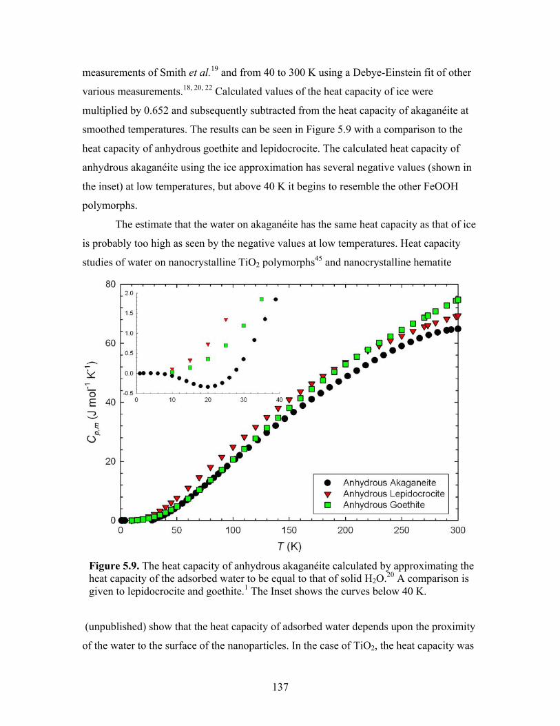
measurements of Smith et al.19 and from 40 to 300 K using a Debye-Einstein fit of other
various measurements.18, 20, 22 Calculated values of the heat capacity of ice were
multiplied by 0.652 and subsequently subtracted from the heat capacity of akaganéite at
smoothed temperatures. The results can be seen in Figure 5.9 with a comparison to the
heat capacity of anhydrous goethite and lepidocrocite. The calculated heat capacity of
anhydrous akaganéite using the ice approximation has several negative values (shown in
the inset) at low temperatures, but above 40 K it begins to resemble the other FeOOH
polymorphs.
The estimate that the water on akaganéite has the same heat capacity as that of ice
is probably too high as seen by the negative values at low temperatures. Heat capacity
studies of water on nanocrystalline TiO2 polymorphs45 and nanocrystalline hematite
(unpublished) show that the heat capacity of adsorbed water depends upon the proximity
of the water to the surface of the nanoparticles. In the case of TiO2, the heat capacity was
Figure 5.9. The heat capacity of anhydrous akaganéite calculated by approximating thheat capacity of the adsorbed water to be equal to that of solid H2O.20 A comparisongiven to lepidocrocite and goethite.1 The Inset shows the curves below 40 K.
e is
137

measured for nanoparticles with varying degrees of hydration, and it was found that the
water on the less hydrated samples had a much lower heat capacity. This can be attributed
to the tighter binding of inner layers9, 10, 45 of water to the surface of the nanoparticles
while the outer layers have more degrees of freedom which correspond to a higher heat
capacity. In general, the heat capacity of water adsorbed onto the surface of both TiO2
and hematite nanoparticles did not equal that of solid H2O. In spite of the poor estimate of
the heat capacity of water on akaganéite, the anhydrous sample shows relatively good
agreement with the other FeOOH polymorphs, and it is possible that some of the water on
akaganéite behaves in a similar manner to solid H2O. Reliable heat capacity studies of
akaganéite with varying degrees of hydration would be useful in providing a better
understanding of the heat capacity of water on the surface of akaganéite which could then
enable a more accurate calculation of the heat capacity of anhydrous akaganéite.
5.4.5 Thermodynamic Functions of Akaganéite (β-FeOOH.0.652H2O)
To calculate thermodynamic functions for akaganéite the semi-adiabatic
m
m
that of the semi-adiabatic. Since the semi-adiabatic technique has a better accuracy
easurements were combined with the PPMS data. A graph of the two sets of
easurements can be seen in Figure 5.5 where below 30 K the PPMS data is higher than
(±0.5%) in this region, the PPMS (±2%) data below 30 K was not included in the
thermodynamic calculations of akaganéite.
The standard molar thermodynamic functions, Cp,m, ΔT0H m, ΔT
0S m, and
Φ m=(ΔT0S m−ΔT
0H m/T) scaled by the ideal gas constant R are reported in Table 5.6 for
hydrated akaganéite (β-FeOOH.0.652H2O). They have been generated at smoothed
temperatures by fitting a combination of orthogonal polynomials (given in Table 5.7) to
the experimental results for akaganéite. These polynomials include the data below 15 K
as they are more convenient in the calculation of the entropy. Although they are not
physically meaningful, these polynomials are a good statistical representation of the he
capacity as can be seen by their respective %RMS values as shown in Table 5.7. The
standard molar entropy of hydrated akaganéite is calculated to be 81.8 ± 2 J.mol-1.K-1,
which is somewhat larger than 59.2 ± 0.2 J.mol-1.K-1 for goethite1 and 65.1 ± 0.2
at
138

J.mol-1.K-1 for lepidocrocite.1 This is most likely due to the contribution from the water in
the entropy calculated for akaganéite while the other polymorphs are anhydrous. With a
etter understanding of the behavior of water on the surface of akaganéite, a more reliable
ron
45
S / R ΔH / RT Φ / R
b
comparison can be made between the stability of akaganéite and the other i
oxyhydroxides.
Table 5.6. Smoothed heat capacity and thermodynamic functions of akaganéite (β-
FeOOH.0.652H2O). Φ = ΔS - ΔH/T, M = 100.938 g/mol, p° = 100 kPa, and R = 8.31
J·K-1·mol-1.
T (K) C / R Δp,m
1.0 5.7694E-05 9.0543E-06 8.2229E-06 6.9131E-06 1.5 0.00018219 5.4659E-05 4.4372E-05 8.5532E-05 2.0 0.00034975 0.00012880 9.8711E-05 0.00025021 2.5 0.00056332 0.00022912 0.00016967 0.00049425 3.0 0.00080209 0.00035266 0.00025493 0.00081255 3.5 0.0010643 0.00049556 0.00035142 0.0011984 4.0 0.0013772 0.00065735 0.00045938 0.0016460 4.5 0.0017708 0.00084141 0.00058240 0.0021535 5.0 0.0022526 0.0010522 0.00072463 0.0027234 5.5 0.0028097 0.0012924 0.00088835 0.0033600 6.0 0.0034280 0.0015631 0.0010738 0.00 06 54 7 6.5 0.0041128 0.0018640 0.0012808 0.0048489 7.0 0.0048965 0.0021966 0.0015103 0.0057067 7.5 0.0058278 0.0025653 0.0017661 0.0066442 8.0 0.0069524 0.0029761 0.0020540 0.0076667 8.5 0.0082974 0.0034368 0.0023807 0.0087818 9.0 0.0098669 0.0039544 0.0027519 0.0099987 9.5 0.011654 0.0045348 0.0031724 0.011328 10 0.013656 0.0051825 0.0036457 0.012779 11 0.018366 0.0066970 0.0047622 0.016087 12 0.024098 0.0085335 0.0061276 0.020004 13 0.030907 0.010724 0.0077646 0.024604 14 0.038907 0.013300 0.0096960 0.029960 15 0.048213 0.016293 0.011946 0.036144 16 0.058913 0 0.043227 .019739 0.014540 17 0.071046 0.023667 0.017500 0.051278
139

18 0.084617 0.028105 0.020844 0.060367 19 0.099614 0.033076 0.024590 0.070556 20 0.11602 0.038596 0.028745 0.081907 25 0.22024 0.074964 0.055978 0.15786 30 0.36661 0.12740 0.094953 0.26979 35 0.54591 0.19714 0.146335 0.42231 40 0.73296 0.28222 0.207962 0.61744 45 0.93434 0.37996 0.277287 0.85377 50 1.1509 0.48951 0.353707 1.1291 55 1.3789 0.60981 0.436466 1.4413 60 1.6162 0.73990 0.524830 1.7882 65 1.8610 0.87890 0.618161 2.1679 70 2.1114 1.0259 0.715846 2.5783 75 2.3656 1.1803 0.817343 3.0175 80 2.6225 1.3412 0.922124 3.4838 85 2.8808 1.5078 1.0297 3.9753 90 3.1392 1.6798 1.1398 4.4905 95 3.3967 1.8565 1.2518 5.0278 100 3.6528 2.0372 1.3654 5.5856 110 4.1574 2.4092 1.5964 6.7574 120 4.6490 2.7920 1.8304 7.9957 130 5.1253 3.1831 2.0657 9.2910 140 5.5854 3.5799 2.3007 10.635 150 6.0296 3.9804 2.5346 12.022 160 6.4588 4.3833 2.7665 13.443 170 6.8747 4.7874 2.9960 14.895 180 7.2787 5.1919 3.2228 16.372 190 7.6724 5.5960 3.4466 17.871 200 8.0566 5.9994 3.6676 19.388 210 8.4321 6.4016 3.8855 20.920 220 8.7981 6.8023 4.1005 22.464 230 9.1533 7.2013 4.3126 24.018 240 9.4949 7.5982 4.5214 25.581 250 9.8192 7.9924 4.7269 27.151 260 10.121 8.3834 4.9286 28.725 270 10.396 8.7707 5.1262 30.302
27 5 3.1 10.475 8.8917 5.1874 30.800 280 10.635 9.1532 5.3188 31.881 290 10.832 9.5300 5.5056 33.461
140

298.15 10.956 9.8320 5.6530 34.746 300 10.979 9.8998 5.6857 35.038
Table summary o hogonal p als used i culation hed heat capacity and therm c functions of akaganéite.
Powers Temperatu e Coef
5.7. A f the ortodynami
olynomi n the cal of smoot
re Rang ficients 1.0 ≤ T (K 6 ) ≤ 11.5 0 0.0 1447 1 -0. 06487 2 0.1 2163 3 -0. 12642 4 0.0 8298 5 -0. 03620 6 0.0 1087 7 -0.0 02295 8 0.00 03451 9 -3.7 08E-05 10 2.8 2E-06 11 -1.4 82E-07 12 5.11 6E-09 13 -1.0 43E-10 14 9.51 1E-13 %RMS = 1.24
11.56 ≤ T (K) ≤
41.11 0 -1.019E+001 1.218E+00 2 -4.855E-01 3 1.007E-01 4 -1.271E-02 5 1.058E-03 6 -6.034E-05 7 2.408E-06 8 -6.764E-08 9 1.329E-09
141

10 -1.782E-11 11 1.554E-13 12 -7.921E-16 13 1.790E-18
%RMS = 0.659
41.11 ≤ T ) ≤ 300 (K 0 -4.547E-01 1 -5.633E-02 2 7.117E-03 3 -4.408E-05 4 8.035E-08 5 2.347E-10 6 -1.126E-12 7 1.181E-15 % RMS = 0.141
Acknowledgements
Portions of the experimental section were written n Lang and Stacey
Smith provided valuable help with the fitting of akagan
References
1. Majzlan, J.; Lang, B. E.; Stevens, R.; Navrotsky eld, B. F.; Boerio-Goates, J., Am. M ral. 2003, 88 -6), 846-854
2. Schwertmann, U., TO ASI Ser., er. C 1988, ils Clay Miner.), 267-308.
3. Schwertmann, U.; Cornell, R. M., on Oxides in tory, 2nd Edition. 2000; p 154
4. Sundman, B., 1991, 12 (2), 127-40. 5. Cornell, R. M.; c ert I on O des: Structure, Properties,
Reactions, Occurr ce a m, 199 p 573. 6. Jambor, J. L.; Dutrizac, J. E., Chem. Rev. (Washington, D. C.) 1998, 98 (7), 2549-
2585. 7. Jansen, E.; Kyek, A.; Schafer, W.; Schwertmann hys. A: Mater. Sci.
Process. 2002, 74 uppl., Pt. 2), S 004-S1006.8. Penn, R. L., Science (Washington, DC, U. S.) 20 2), 1704-1705. 9. Navrotsky, A., J. Chem. Thermodyn. 2006, 39 (1
by Dr. Bria
éite.
, A.; Woodfiine (5 . NA S 217 (Iron So
Ir the Labora
J. Phase Equilib. S hw
enmann, U.; Editors, Thend Uses. VCH: Weine
r xi6;
, U., Appl. P (S 1
07, 316 (583), 2-9.
142

10. Navrotsky, A.; Mazeina, L.; Majzlan, J., Science (Washington, DC, U. S.) 2008, 319 (5870), 1635-1638.
11. Ott, J. B.; Boerio-Goates, J., Applications. 200 p 360
2. Lang, B. E. Specific Heat and Thermodynamic Properties of Metallic Systems: n and Analysis. 2005.
Am. Mineral. 2003, 88 (5-6), 855-859. 4. .
smochim. Acta 2007, 71 (3),
6. Majzlan, J.; Navrotsky, A.; Schwertmann, U., Geochim. Cosmochim. Acta 2004, 68 (5), 1049-1059.
17. Majzlan, J.; Navrotsky, A.; W Lang, B. E.; Boerio-Goates, J.;
. 1974, 6 (9), 815-
(12),
.;
Chemical Thermodynamics: Principles and pp. 0;
1Instrumentatio
13. Majzlan, J.; Grevel, K.-D.; Navrotsky, A., 1 Majzlan, J.; Koch, C. B.; Navrotsky, A., Clays Clay Miner. 2008, 56 (5), 526-53015. Majzlan, J.; Mazeina, L.; Navrotsky, A., Geochim. Co
615-623. 1
oodfield, B. F.; Fisher, R. A., J. Low Temp. Phys. 2003, 130 (1/2), 69-76.
18. Giauque, W. F.; Stout, J. W., J. Am. Chem. Soc. 1936, 58, 1144-50. Smith, S. J.; Lang, B. E.; Liu, S.; Boerio-Goates, J19. .; Woodfield, B. F., J. Chem. Thermodyn. 2007, 39 (5), 712-716. Flubacher20. , P.; Leadbetter, A. J.; Morrison, J. A., J. Chem. Phys. 1960, 33, 1751-5.
21. Wei, C.; Wang, X.; Nan, Z.; Tan, Z., J. Chem. Eng. Data 2009, 55 (1), 366-369Haida, O.; Ma22. tsuo, T.; Suga, H.; Seki, S., J. Chem. Thermodyn. 25.
23. Ewing, F. J., J. Chem. Phys. 1935, 3, 420-4. Morris, R. V.; Lauer, H. V., Jr.; Lawson, C. A.; Gibson, E. K., J24. r.; Nace, G. A.; Stewart, C., J. Geophys. Res., B 1985, 90 (B4), 3126-44. Hall, P25. . G.; Clarke, N. S.; Maynard, S. C. P., J. Phys. Chem. 1995, 99 (15), 5666-73. Hirt, A. M.; Lanci, L.; Dobson, J.; Weidler, P.; G26. ehring, A. U., J. Geophys. Res., [Solid Earth] 2002, 107 (B1), EPM5/1-EPM5/9.
27. Murad, E.; Schwertmann, U., Mineral. Mag. 1984, 48 (349), 507-11. 28. Murad, E., Clay Miner. 1979, 14 (4), 273-83.
Cai, J.; Liu, J.; Gao, Z.; Navrotsky, A.; Suib, S. L., 29. Chem. Mater. 2001, 134595-4602. Barrero, C. A.; Garcia, K. E.; M30. orales, A. L.; Kodjikian, S.; Greneche, J. M., J. Phys.: Condens. Matter 2006, 18 (29), 6827-6840. Chambaere, D.; De Grave, E., J. Mag31. n. Magn. Mater. 1984, 42 (3), 263-8.
32. Sherman, D. M., Geochim. Cosmochim. Acta 2005, 69 (13), 3249-3255. 33. Gopal, E. S. R., Specific Heats at Low Temperatures (International Cryogenics
Monograph Series). Plenum Press: New York, 1966; p 226 Lang, B. E34. .; Boerio-Goates, J.; Woodfield, B. F., J. Chem. Thermodyn. 2006, 38 (12), 1655-1663. Stevens, R.; Boerio-35. Goates, J., J. Chem. Thermodyn. 2004, 36 (10), 857-863.
36. Lashley, J. C.; Lang, B. E.; Boerio-Goates, J.; Woodfield, B. F.; Darling, T. WChu, F.; Migliori, A.; Thoma, D., J. Chem. Thermodyn. 2002, 34 (2), 251-261.
37. Gronvold, F.; Westrum, E. F., Jr., J. Am. Chem. Soc. 1959, 81, 1780-3. 38. Phillips, N. E., Crit. Rev. Solid State Sci. 1971, 2 (4), 467-553.
143
39. Fisher, R. A.; Bouquet, F.; Phillips, N. E.; Franck, J. P.; Zhang, G.; Gordon, J. E.;
25/1-134425/9.
4.
4. ust. J.
(4), 750-754.
Marcenat, C., Phys. Rev. B: Condens. Matter Mater. Phys. 2001, 64 (13), 1344
40. Niira, K., Phys. Rev. 1960, 117, 129-33. 41. Boerio-Goates, J.; Stevens, R.; Lang, B.; Woodfield, B. F., J. Therm. Anal.
Calorim. 2002, 69 (3), 773-783. 42. Coey, J. M. D.; Von Molnar, S.; Torressen, A., J. Less-Common Met. 1989, 151,
191-43. Lee, G. H.; Kim, S. H.; Choi, B. J.; Huh, S. H.; Chang, Y.; Kim, B.; Park, J.; Oh,
S. J., J. Korean Phys. Soc. 2004, 45 (4), 1019-10244. Childs, C. W.; Goodman, B. A.; Paterson, E.; Woodhams, F. W. D., A
Chem. 1980, 33 (1), 15-26. 45. Boerio-Goates, J.; Li, G.; Li, L.; Walker, T. F.; Parry, T.; Woodfield, B. F., Nano
Lett. 2006, 6
144

Chapter 6
The Effects of Imidazole, MOPS, and Cysteine Buffers
on the Reconstitution of the Iron Core of Horse Spleen
Ferritin
6.1 Introduction The use of proteins as a template for the production of nanomaterials is an
emerging and promising aspect of biochemical engineering.1, 2 Research in materials
science has assimilated the concepts of biology on a basic level, and now faces the
challenge of carrying this knowledge over to applied materials. Facilitating discovery in
this discipline is attractive for many reasons. For example, protein cages are among just a
few nanoplatforms capable of simultaneous control over size, shape, and
biocompatibility.3 Studies have shown that, in nature, protein interactions not only direct
nucleation of inorganic materials, but also control the crystal type, face, and size, even of
metastable forms, all in aqueous solutions and at ambient conditions.1, 3 Furthermore,
protein cages yield products which are already dispersed in solution and thus avoid the
problem of agglomeration common in other production methods. Proteins are also
attractive because they are amenable to alterations in functionality through both chemical
and genetic means.
Ferritin, the biological protein for iron storage,4 has been more extensively studied
as a nanoplatform than any other protein, and not without success. Mn(O)OH, Mn3O4,
Co(O)OH, Co3O4, Cr(OH)3, Ni(OH)3, In2O3, FeS, CdS, CdSe, and ZnSe have all been
synthesized within the ferritin protein cage.1, 5-12 Metallic nanoparticles such as Pd, Ag,
and CoPt have also been synthesized within ferritin by pre-incubation of the protein with
a metal salt and subsequent chemical reduction by a strong reducing agent.3 Compounds
145

formed in ferritin have shown promise in catalysis, electrochemistry, and targeted drug
delivery and bioimaging.1, 3, 5, 12
Ferritin is a spherical protein cage with an outer diameter of 12 nm and an interior
cavity of 8 nm.4 The shell is composed of 24 subunits that self-assemble generating
channels of 4 Ǻ in diameter, eight of which are hydrophilic. Ferritin has been observed to
contain as many as 4500 iron atoms although naturally the average is closer to 2000.
These iron atoms form a ferric oxyhydroxide core in the center of the ferritin cavity that
most resembles ferrihydrite.13-15 The solid iron core can be chemically removed through
chemical reduction followed by chelation and dialysis.16, 17
It has been shown that chemical species in solution such as buffers and salts can
greatly affect iron uptake in ferritin for in vitro reactions.18 Studies by Cutler et al.19
concluded that, in general, cations slow the rate of iron loading into ferritin by competing
with Fe2+ for negatively charged amino acids. Specific anions such as halides and sulfate
had no effect. On the other hand phosphate and its tetrahedral oxo-anion analogs have
been shown to stimulate the rate of iron loading into ferritin.20-23 Pâques et al.24 studied
the effects of buffer, ionic strength, pH, and temperature upon the rate of core formation
in ferritin. This study involved the buffers 4-morpholinoepropanesulphonic acid (MOPS),
4-morpholineethanesulphonic acid (MES), and imidazole. At lower pH’s the authors
concluded that there was little difference in the rates for these buffers, but at a pH of 7.0
imidazole showed much smaller rates of iron formation. These authors also observed an
inhibition of ferritin core formation with increasing ionic strength which is consistent
with the findings of Cutler et al.19 as to the general effects of cations and anions.
Oxidative damage to apoferritin results in the termination of core formation and
presents a serious problem when trying to maximize the number of iron atoms introduced
into the protein.4, 25 In the natural process of core formation, Fe2+ is oxidized at the
ferroxidase center and subsequently solidifies in the central cavity. If the Fe2+ were to be
oxidized before entering the protein’s channels,26 hydroxyl radicals27 would be produced
through the well-known Fenton reaction. The production of these radicals damages the
ferritin protein and prevents iron core formation.28
Although Pâques24 and his coworkers theorized that complexing ions like
imidazole inhibit core formation, complexing ions may prevent the premature oxidation
146

of Fe2+. Pâques et al. suggested that inhibition was due to the binding of complexing ions
to the active site of apoferritin and did not discuss the idea of oxidative damage. This
study revisits the effects of buffers on iron loading in ferritin with the aim of maximizing
iron content in ferritin. A report is given of the effects of MOPS, imidazole, and cysteine.
6.2 Experimental
6.2.1 Preparation of Apoferritin
Native horse spleen ferritin (HoSF) obtained from Sigma-Aldrich was treated
according to established methods to make apoferritin.29 As obtained HoSF in saline
solution was dialyzed for 24 hours against 1% thioglycolic acid and 0.25 M sodium
acetate (NaC2H3O2) at 4°C. This process was repeated with an addition of 100 mg/L of
2,2’ bipyridyl (bipy) which chelates Fe2+ forming the red [Fe(bipy)3]2+ complex. The
HoSF was then dialyzed twice with 5 g/L sodium bicarbonate (NaHCO3) at 4°C. The
apoferritin solution was then dialyzed several times with H2O at 4°C to remove ionic
species from the solution. Dialysis with H2O was terminated when Na, S, C, and Fe could
not be detected in the rinsing solution.
6.2.2 Study of Core Formation in MOPS, Cysteine, and Imidazole
Kinetic studies on the iron-loading in ferritin were carried out on an Agilent 8453
UV-Vis spectrometer equipped with a magnetic stirring motor, and changes in the
absorbance at 310 nm were monitored. Imidazole (C3H4N2), cysteine (HO2C2H3N), and
MOPS solutions (0.05 M) were prepared and the pH adjusted to 7.5 by the addition of
NaOH for MOPS and cysteine and HNO3 for imidazole. A 0.010 M Fe2+ solution was
prepared by the combination of 49.7 mg Fe(NH4)2(SO4)2.6H2O with 5 mL of 1 mM HCl
and 5 mL of H2O. Reaction solutions were prepared in a cuvette with 1.8 mL of buffer
and 20 µL of 1.2 x 10⁻⁵ M apoferritin and a Teflon coated stir bar. Absorbance was
measured over time at 310 nm, and once a baseline was established 40 µL of 0.010 M
Fe2+ was quickly injected into the cuvette. The absorbance measurements were continued
for 10 minutes.
147

6.2.3 Preparation and Characterization of Reconstituted Ferritin in MOPS and
Imidazole
A reconstituted ferritin sample was prepared in the presence of imidazole buffer.
Imidazole (1.65 g) was combined with apoferritin in a 350 mL solution. The pH was
adjusted to 7.5 by the addition of HNO3(aq). An Fe2+ solution was prepared by dissolving
2.01 g Fe(NH4)2(SO4)2.6H2O in 880 mL H2O with 0.475 mL 1 M HCl. The Fe2+ solution
was slowly titrated into the apoferritin solution at room temperature under constant
stirring, and the pH was monitored and maintained at 7.5 by the addition of NaOH(aq).
As the titration progressed the solution turned to a dark brownish-red. After ~ 16 hours, a
small amount of solid began to form and the reaction was stopped. The solid was
removed by centrifugation, and the ferritin solution was transferred to a dialysis bag. The
ferritin was dialyzed at 4°C with water to remove all salts and impurities. The water from
each round of dialysis was analyzed for S, Na, C, and Cl-. The Na was analyzed by
atomic absorption spectrometry (AA), while S and C were analyzed using inductively
coupled plasma optical emission spectrometry (ICP-OES), and the Cl- was quantified
using ion chromatography (IC). Once the levels of these species were below detection
limits the ferritin solution was removed and lyophilized. The mass of the recovered
product was 435.7 mg. The iron content of this powder was analyzed by ICP-OES and
the crystallinity of the core was characterized by powder X-ray diffraction (XRD) using a
Scintag Diffractometer (Cu-Kα radiation, λ = 1.54176 nm) at a scanning rate of 0.1
2θ/min and a power of 15 kW over the range 10 to 85°.
A second ferritin sample was prepared in a MOPS solution. An apoferritin
solution (24 mL) was combined with 3.139 g MOPS, 0.4383 g NaCl, and 150 mL H2O.
The pH of this solution was adjusted to 7.5 by the addition of NaOH(aq). A Fe2+ solution
was prepared by dissolving 312.8 mg Fe(NH4)2(SO4)2.6H2O in 138 mL of 1 mM HCL.
The two solutions were combined in the same manner as the imidazole reaction with
constant stirring and maintenance of the pH at 7.5. The reaction was stopped after ~ 8
hours when the mixture began to get cloudy due to protein precipitation. The solid was
removed by centrifugation and the buffer exchanged to water by dialysis which also
removed any salts. Rinsing was terminated after the impurities were no longer detected
by the same methods described in the preparation of the imidazole sample. The solution
148

was then lyophilized yielding 0.176 g, and the powder was analyzed using ICP-OES and
XRD.
6.3 Results and Discussion
Iron loading into ferritin was monitored by following the absorbance at 310 nm in
the various buffers and the results are shown in Figure 6.1. The curve representing the
reaction in MOPS is characterized by a sigmoidal shape which has been described
previously by Xu and Chasteen.30, 31 This shape is due to two different iron loading
reactions. The first occurs at low iron content in ferritin where Fe2+ is oxidized at the
ferroxidase center. As a core begins to form inside ferritin, Fe2+ can be oxidized on the
surface of the growing mineral core. As the surface area of the core increases, iron
oxidation also increases resulting in the sigmoidal shape. Conversely, the curve
representing the reaction in imidazole rises exponentially before reaching a plateau. This
behavior suggests that the iron is entering the ferritin protein and reacting at an
accelerated rate. Interestingly, the reaction in cysteine never reaches the final level of
absorbance observed in the other reactions in spite of a sharp rise at the beginning. The
reaction in cysteine was repeated in the absence of ferritin and the results can be seen in
Figure 6.2. In this curve the absorbance rises almost instantaneously then decays to a
constant absorbance. This suggests that the cysteine initially complexes with all the iron
and then progresses to an equilibrium between iron bound to ferritin and an Fe(cysteine)x
complex in solution. Because of this equilibrium, cysteine was not selected in preparing
powdered samples of reconstituted ferritin.
Table 6.1 shows the
ICP-OES results for iron
content in the imidazole and
MOPS samples. The iron
content is reported in two
ways. The first number describes the moles of iron found in one gram of the lyophilized
powder while the second quantifies the number of iron atoms in one ferritin protein. This
second number is found if we assume a formula of FeOOH for the mineral core and that
the rest of the mass is the apoferritin protein which has a molecular weight of 450 kDa.4
Table 6.1. Iron content for the two ferritin powders determined by ICP-OES.
Sample Moles Fe/gram sample
Moles Fe/protein
Imidazole Ferritin 4.12(4) x 10-3 2956 MOPS Ferritin 2.82(0) x 10-3 1693
149

Figure 6.1. The absorbance at 310 nm over time as a probe of core formation. The reaction was initiated by injecting a Fe2+ solution into the solution in the cuvette under constant stirring.
In this table, the imidazole sample shows a higher iron content of 2956 Fe/protein while
the MOPS sample has 1693. The higher iron content in the imidazole sample is consistent
with the exponential rise shown in the UV-Vis experiments. These results contradict
those of Pâques et al.24 who concluded that at a pH of 7.0 and high ionic strength,
imidazole inhibits core formation. However, the reactions in the present study were
carried out at a pH of 7.5 which is somewhat higher, and it is possible that there is a
crossover in pH where imidazole is less inhibitory. Such a crossover could explain the
difference between the two studies.
150

Figure 6.2. The absorbance at 310 nm of Fe2+ ion injected into a cysteine solution in the absence of apoferritin.
An XRD spectrum in the range 5 to 85o for a lyophilized sample of apoferritin can
be found in Figure 6.3. Two reflections are observed at 2θ values of 9.72o, and 19.80o.
After the second peak the spectrum decays with no other features. This spectrum can be
seen as a background in the XRD spectra of the two reconstituted ferritin powders found
in Figures 6.4 and 6.5, respectively. Figure 6.4 shows the XRD spectrum from the
sample prepared in imidazole with the reference peaks for the reflections of six-line
ferrihydrite found in JCPDS card 00-029-0712.32 In addition to the apoferritin
background, the XRD of this sample shows peaks which correspond to 6-line ferrihydrite.
The two broad peaks located around 35o and 63o indicate that while 6-line ferrihydrite is
present, it is mixed with the less-ordered 2-line ferrihydrite, which displays only two
broad reflections at these angles.32 Figure 6.5 contains the XRD spectrum for the ferritin
sample reconstituted in MOPS. The smaller amount of sample produces the effect of a
lower intensity, however some key features can be discerned. The spectrum has the
characteristic curve of the apoferritin XRD spectrum which interferes with the pattern of
the iron core. In spite of this interference a definite broad peak is observed ranging from
57 to 66o which corresponds with 2-line ferrihydrite. Other possible peaks are found
151

Figure 6.3. Powder X-ray Diffraction (XRD) spectrum of lyophilized apoferritin powder.
at 35o, 46o, and 53o. Peaks at these locations suggest that 6-line ferrihydrite is beginning
to form. A comparison of the two spectra reveals that the core of ferritin prepared in
imidazole has greater order as seen by the more distinct peaks in its XRD spectrum.
6.4 Conclusion
In conclusion buffer effects on the formation of the ferritin core were studied by
measuring the absorbance at 310 nm over time using UV-Vis spectroscopy.
Complexation by cysteine may inhibit the uptake of iron as experiments without ferritin
showed a sharp rise followed by a slow decay to a constant absorbance. Iron uptake in
imidazole was exponential and leveled quickly while reactions in MOPS were slower and
had a sigmoidal character. This evidence points to imidazole facilitating the introduction
of iron into the ferritin protein. Quantitative analysis of iron in lyophilized samples
152

Figure 6.4. XRD spectrum of a ferritin sample reconstituted in imidazole. The red lines represent the standard pattern for 6-line ferrihydrite.
revealed a greater number of iron atoms could be introduced into ferritin using imidazole
than could be achieved in the presence of MOPS. XRD spectra of these samples shows a
cleaner spectrum with more diffuse peaks for the sample prepared in imidazole. The
spectrum of the sample reconstituted in imidazole was found to most likely to have a core
consisting of a mixture of 2-line and 6-line ferrihydrite. The greater number of iron atoms
introduced into the ferritin protein suggests that imidazole stabilizes Fe2+, keeps it in the
solution for a longer duration, and prevents the damage to the ferritin protein by free
radicals. These results also suggest that, in addition to the effects of chemical species on
the rate of core formation, buffers and salts can affect the final size of the iron core in
ferritin.
153

Figure 6.5. XRD spectrum of ferritin reconstituted in MOPS. The red lines represent the standard pattern for 6-line ferrihydrite.
References
1. Katz, E.; Willner, I., Angewandte Chemie, International Edition 2004, 43 (45), 6042-6108.
2. Iwahori, K.; Yamashita, I., Recent Res. Dev. Biotechnol. Bioeng. 2005, 7, 41-68. 3. Uchida, M.; Klem, M. T.; Allen, M.; Suci, P.; Flenniken, M.; Gillitzer, E.;
Varpness, Z.; Liepold, L. O.; Young, M.; Douglas, T., Advanced Materials (Weinheim, Germany) 2007, 19 (8), 1025-1042.
4. Arosio, P.; Ingrassia, R.; Cavadini, P., Biochim. Biophys. Acta, Gen. Subj. 2009, 1790 (7), 589-599.
5. Bulte, J. W.; Douglas, T.; Mann, S.; Frankel, R. B.; Moskowitz, B. M.; Brooks, R. A.; Baumgarner, C. D.; Vymazal, J.; Strub, M. P.; Frank, J. A., Journal of magnetic resonance imaging JMRI 1994, 4 (3), 497-505.
6. Dominguez-Vera, J. M.; Colacio, E., Inorg. Chem. 2003, 42 (22), 6983-6985. 7. Douglas, T.; Dickson, D. P. E.; Betteridge, S.; Charnock, J.; Garner, C. D.; Mann,
S., Science (Washington, D. C.) 1995, 269 (5220), 54-7. 8. Gerion, D.; Pinaud, F.; Williams, S. C.; Parak, W. J.; Zanchet, D.; Weiss, S.;
Alivisatos, A. P., Journal of Physical Chemistry B 2001, 105 (37), 8861-8871. 9. Iwahori, K.; Yoshizawa, K.; Muraoka, M.; Yamashita, I., Inorg. Chem. 2005, 44
(18), 6393-6400. 10. Meldrum, F. C.; Heywood, B. R.; Mann, S., Science (Washington, DC, United
States) 1992, 257 (5069), 522-3. 11. Yamashita, I.; Hayashi, J.; Hara, M., Chemistry Letters 2004, 33 (9), 1158-1159.
154

12. Sanchez, P.; Valero, E.; Galvez, N.; Dominguez-Vera, J. M.; Marinone, M.; Poletti, G.; Corti, M.; Lascialfari, A., Dalton Transactions 2009, (5), 800-804.
13. Allen, M.; Douglas, T.; Nest, D.; Schoonen, M.; Strongin, D., ACS Symp. Ser. 2005, 890 (Nanotechnology and the Environment), 226-229.
14. Gorham, N. T.; Pierre, T. G. S.; Chua-Anusorn, W.; Parkinson, G. M., J. Appl. Phys. 2008, 103 (5), 054302/1-054302/5.
15. Kim, S.-W.; Seo, H.-Y.; Lee, Y.-B.; Park, Y. S.; Kim, K.-S., Bull. Korean Chem. Soc. 2008, 29 (10), 1969-1972.
16. Joo, M. S.; Tourillon, G.; Sayers, D. E.; Theil, E. C., Biol. Met. 1990, 3 (3-4), 171-5.
17. Granick, S.; Michaelis, L., J. Biol. Chem. 1943, 147, 91-7. 18. Yang, X.; Chasteen, N. D., Biochem. J. 1999, 338 (3), 615-618. 19. Cutler, C.; Bravo, A.; Ray, A. D.; Watt, R. K., J. Inorg. Biochem. 2005, 99 (12),
2270-2275. 20. Cheng, Y. G.; Chasteen, N. D., Biochemistry 1991, 30 (11), 2947-53. 21. Aitken-Rogers, H.; Singleton, C.; Lewin, A.; Taylor-Gee, A.; Moore, G. R.; Le
Brun, N. E., JBIC, J. Biol. Inorg. Chem. 2004, 9 (2), 161-170. 22. Orino, K.; Kamura, S.; Natsuhori, M.; Yamamoto, S.; Watanabe, K., BioMetals
2002, 15 (1), 59-63. 23. Polanams, J.; Ray, A. D.; Watt, R. K., Inorg. Chem. 2005, 44 (9), 3203-3209. 24. Paques, E. P.; Paques, A.; Crichton, R. R., Eur. J. Biochem. 1980, 107 (2), 447-
53. 25. Orino, K.; Lehman, L.; Tsuji, Y.; Ayaki, H.; Torti, S. V.; Torti, F. M., Biochem. J.
2001, 357 (1), 241-247. 26. Rohrer, J. S.; Frankel, R. B.; Papaefthymiou, G. C.; Theil, E. C., Inorg. Chem.
1989, 28 (17), 3393-5. 27. Yoon, J. H.; Kang, J. H., Bull. Korean Chem. Soc. 2009, 30 (7), 1644-1646. 28. Linder, M. C.; Kakavandi, H. R.; Miller, P.; Wirth, P. L.; Nagel, G. M., Arch.
Biochem. Biophys. 1989, 269 (2), 485-96. 29. Treffry, A.; Harrison, P. M., Biochem. J. 1978, 171 (2), 313-20. 30. Hanna, P. M.; Chen, Y.; Chasteen, N. D., J. Biol. Chem. 1991, 266 (2), 886-93. 31. Xu, B.; Chasteen, N. D., J. Biol. Chem. 1991, 266 (30), 19965-70. 32. Drits, V. A.; Sakharov, B. A.; Salyn, A. L.; Manceau, A., Clay Miner. 1993, 28
(2), 185-207.
155