Ocean Modelling 61 (2013) 49–67

Contents lists available at SciVerse ScienceDirect

Ocean Modelling

journal homepage: www.elsevier .com/locate /ocemod

The Gulf of Cadiz–Alboran Sea sub-basin: Model setup, exchange andseasonal variability

Alvaro Peliz a,b,⇑, Dmitri Boutov b, Rita M. Cardoso a,1, Javier Delgado c, Pedro M.M. Soares a,2

a IDL, Universidade de Lisboa, Lisbon, Portugalb Centro de Oceanografia, Universidade de Lisboa, Lisbon, Portugalc Physical Oceanography Group, University of Malaga, Malaga, Spain

a r t i c l e i n f o

Article history:Received 27 June 2012Received in revised form 3 October 2012Accepted 17 October 2012Available online 10 November 2012

Keywords:Gulf of Cadiz–Alboran Sea sub-basinStrait of Gibraltar exchangeWestern MediterraneanROMSWRF

1463-5003/$ - see front matter � 2012 Elsevier Ltd. Ahttp://dx.doi.org/10.1016/j.ocemod.2012.10.007

⇑ Corresponding author at: IDL, Universidade de L+351 21 7500143; fax: +351 21 7500009.

E-mail address: ajpeliz@fc.ul.pt (A. Peliz).1 Tel.: +351 21 7500143; fax: +351 21 7500009.2 Tel.: +351 21 7500143; fax: +351 21 7500009.

a b s t r a c t

A high resolution (�2 km) 20-year simulation forced with a high resolution (�9 km) winds and air–seafluxes covering the Gulf of Cadiz and the Alboran Sea is described. The across-strait mass flux becomesa critical issue and the strategy that was adopted towards a correct implementation of the exchange isreported. A net transport previously calculated is forced in the barotropic mode through the boundaries,and the model is left free to adjust the exchange (inflow/outflow) to the imposed mass flux. A thoroughlycomparison of the model results with observations and other exchange estimates are provided and newvalues are proposed. The model reproduces the main modes of outflow variability with statistics almostidentical to the observed ones (0:78� 0:09 Sv). For the inflow, the model values (0:83� 0:056 Sv) arecompared with observations and new estimates are provided and analyzed. Despite the fact that the mix-ing processes inside the strait are under-resolved, the product water masses to the west (Mediterraneanoutflow) and to the east (Atlantic Water – inflow) are well represented in the model. The mean circula-tion features are described and compared with observations from a few long-term moorings, and ana-lyzed in light of existing literature.

� 2012 Elsevier Ltd. All rights reserved.

1. Introduction coupling in the Gulf of Cadiz (see recent works of Peliz et al.

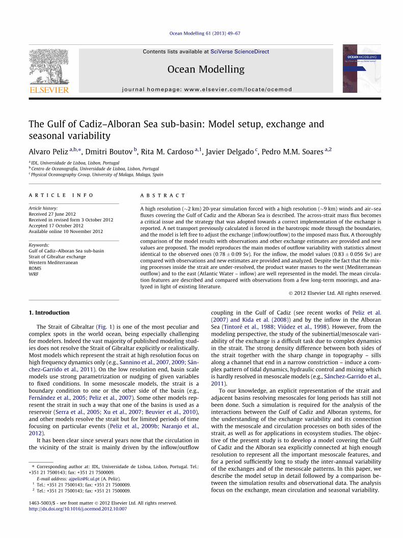
The Strait of Gibraltar (Fig. 1) is one of the most peculiar andcomplex spots in the world ocean, being especially challengingfor modelers. Indeed the vast majority of published modeling stud-ies does not resolve the Strait of Gibraltar explicitly or realistically.Most models which represent the strait at high resolution focus onhigh frequency dynamics only (e.g., Sannino et al., 2007, 2009; Sán-chez-Garrido et al., 2011). On the low resolution end, basin scalemodels use strong parametrization or nudging of given variablesto fixed conditions. In some mesoscale models, the strait is aboundary condition to one or the other side of the basin (e.g.,Fernández et al., 2005; Peliz et al., 2007). Some other models rep-resent the strait in such a way that one of the basins is used as areservoir (Serra et al., 2005; Xu et al., 2007; Beuvier et al., 2010),and other models resolve the strait but for limited periods of timefocusing on particular events (Peliz et al., 2009b; Naranjo et al.,2012).

It has been clear since several years now that the circulation inthe vicinity of the strait is mainly driven by the inflow/outflow

ll rights reserved.

isboa, Lisbon, Portugal. Tel.:

(2007) and Kida et al. (2008)) and by the inflow in the AlboranSea (Tintoré et al., 1988; Viúdez et al., 1998). However, from themodeling perspective, the study of the subinertial/mesoscale vari-ability of the exchange is a difficult task due to complex dynamicsin the strait. The strong density difference between both sides ofthe strait together with the sharp change in topography – sillsalong a channel that end in a narrow constriction – induce a com-plex pattern of tidal dynamics, hydraulic control and mixing whichis hardly resolved in mesoscale models (e.g., Sánchez-Garrido et al.,2011).

To our knowledge, an explicit representation of the strait andadjacent basins resolving mesoscales for long periods has still notbeen done. Such a simulation is required for the analysis of theinteractions between the Gulf of Cadiz and Alboran systems, forthe understanding of the exchange variability and its connectionwith the mesoscale and circulation processes on both sides of thestrait, as well as for applications in ecosystem studies. The objec-tive of the present study is to develop a model covering the Gulfof Cadiz and the Alboran sea explicitly connected at high enoughresolution to represent all the important mesoscale features, andfor a period sufficiently long to study the inter-annual variabilityof the exchanges and of the mesoscale patterns. In this paper, wedescribe the model setup in detail followed by a comparison be-tween the simulation results and observational data. The analysisfocus on the exchange, mean circulation and seasonal variability.

o o o o o 10 W 8 W 6 W 4 W 2 W 0o

35oN

36oN

37oN

38oN

St. Gib

C.TF

Al

Or

CSMCSV

A

CG

P

Gulf of Cadiz

Alboran Sea

Fig. 1. Map of the model domain with model topography (plotted every 500 m in blue, and the isobaths 0–250 m every 50 m in black). The geographical sites are thefollowing: CSV – Cape St. Vicente; CSM – Cape Sta. Maria; St. Gib – Strait of Gibraltar; Al – Almeria; C.TF – Cape Tres Forcas; and Or – Oran. The red stars indicate the positionsof the long-term surface meteo and oceanographic buoys (deployed and maintained by Insituto Puertos del Estado – Spain) used in this study: C – Cadiz; A – Alboran; G – Gataand P – Palos. The red dots inside the strait indicate the location of the two main sills: Espartel (the western one) and Camarinal (on the east). (For interpretation of thereferences to color in this figure legend, the reader is referred to the web version of this article.)

50 A. Peliz et al. / Ocean Modelling 61 (2013) 49–67

2. Model description

2.1. The ocean model, domain and configuration

The simulations were performed using the Regional OceanModeling System (ROMS), which is a community model designedfor regional realistic applications (e.g., Shchepetkin and McWil-liams, 2005). ROMS kernel is a 3D free-surface, sigma-coordinate,split-explicit primitive equation model with Boussinesq andhydrostatic approximations.

The ocean model domain (Fig. 1) has been chosen in order to in-clude the coupling of the inflow/outflow and the development ofthe Gulf of Cadiz slope Current (GCC; Peliz et al., 2007) on the east,and the recurrent mesoscale features on the Alboran side: the Wes-tern Alboran Gyre (WAG) and Eastern Alboran Gyre (EAG), theAlmeria-Oran front, and the beginning of the Algerian Currentwhere occasionally a third Gyre is observed (see Tintoré et al.(1988) and Millot (1999) for a detailed characterization of thesefeatures). The extension of the domain to the east is associatedwith the occurrence of strong mesoscale activity in the transitionbetween the Alboran Sea and the Algerian–Balearic basin.

The model grid (Fig. 1) has a � 2 � 2 km resolution and 32 sig-ma vertical levels (Shchepetkin and McWilliams, 2005) with amoderate surface stretching of hs = 4 (hb ¼ 0) to keep a reasonableresolution near the bottom, which is important for the outflow onthe Gulf of Cadiz slope (see Hedstrom (2009) Appendix B for a de-tailed description of ROMS vertical coordinates). An alternativeway of increasing the near-bottom resolution is to use a hb differ-ent from zero. However, this option increases the steepness of thesigma layers, with the consequence of larger pressure gradient er-rors (Shchepetkin et al., 2003). The baroclinic time-step dt is 200 s,and the fast barotropic mode is dt=40 ¼ 5 s.

2.2. Boundary conditions

2.2.1. Baroclinic boundary conditionsThe open boundary conditions are a combination of outward

radiation and flow-adaptive nudging toward prescribed externalconditions from climatology as described in Marchesiello et al.(2001). Climatological monthly values of temperature and salinity,together with geostrophic and Ekman velocities (calculated basedon seasonally averaged stratification and surface winds) are usedon the boundary as passive/active conditions (Marchesiello et al.,2001). Nudging to climatological values is made with differentcoefficients for inward (1 day for momentum and 10 days for trac-ers)/outward flow (360 days for tracers and momentum). Across

the nudging/sponge band, the nudging progressively decays tozero in the interior. The initial and open boundary temperatureand salinity fields were taken from the MEDATLAS (MEDAR Group2002), for the Mediterranean side and from the WOA2005(www.nodc.noaa.gov/OC5/WOA05) for the Atlantic. Climatologyis used in a 40 km wide restoring band along the boundaries coin-cident with the band used for the sponge (see Section 2.4).

The use of climatological boundaries excludes the representa-tion of part of the remote variability in the system. On one hand,coastaly guided perturbations traveling along the ocean marginswhich may have some significance on the southwestern and north-eastern parts of the domain are not represented. However, theexisting literature does not cover these processes in a systematicway, and it is difficult to evaluate how far their misrepresentationcan affect our model results. On the other hand, the remote vari-ability associated with inter-annual and long period changes inthe circulating water masses (and thus water column structure)are not considered in this model.

In the past decade, an increasing attention has been devoted tothe study of inter-annual variability of winter water mass forma-tion on the Eastern and Northwestern Mediterranean. Importantmodes of water mass variability and thermohaline circulation likethe Eastern Mediterranean Transient (EMT) and Western Mediter-ranean Transition (WMT) are the core of present Mediterraneancirculation studies (Roether et al., 1996; Zervakis et al., 2004; Zun-ino et al., 2012). However, the impact of these events on the wes-tern basin is still ongoing work. The propagation of theseanomalies through the western Mediterranean is still being fol-lowed over the last years (e.g., Schroder et al., 2006). The way theywill affect the Alboran Sea is still an open question. In future, theuse of Mediterranean-scale reanalysis will allow to assess the im-pact of these fluctuations in the water mass structures arriving inthe Alboran on the inflow/outflow system. Presently, the existinginformation is rather insufficient and in this study it was decidedto use climatological temperature and salinity data instead.

2.2.2. The barotropic condition and volume conservationFor the barotropic mode we use Orlansky radiative conditions

(e.g., Haidvogel and Beckmann, 1999) together with volume con-servation. ROMS volume conservation condition consists of diag-nosing the mass imbalance at each time step (by integrating allthe barotropic transport along the domain perimeter). In case themodel is losing volume a correction is done by dividing the ex-cess/deficit by all cells along the open boundaries and forcing thismass out/in as a volume compensation. A correct implementationacross the strait requires that this condition is applied to each

A. Peliz et al. / Ocean Modelling 61 (2013) 49–67 51

basin separately. Otherwise, the mass compensation induces un-wanted and spurious barotropic fluctuations in the strait thatsometimes are well above the observed values. In this configura-tion, we proceeded with the separation of the volume condition.At each time step the barotropic transport was calculated for theAtlantic side (Q Atl) and for the Mediterranean (QMed), indepen-dently. Next, assuming volume conservation, we force the trans-port entering/leaving on the Atlantic boundary be equal to thetransport leaving/entering on the open boundary in the Mediterra-nean side, and this transport should equal Qt – the net (physical)mass transport through the strait. This approach ensures volumeconservation and the needed subinertial barotropic transportacross the strait. The internal baroclinic adjustment of the modelto this external barotropic forcing will determine part of the subin-ertial inflow/outflow fluctuations.

2.3. Mediterranean mass balance and Q t

Our model domain covers the Mediterranean only marginally,but the variability inside the Mediterranean will affect our studyarea in a drastic way through mass flux forcing. On synoptic andseasonal scales, the inflow/outflow is forced by sea-level changeson the Mediterranean side. These sea-level fluctuations are com-pensated by the net flow through the strait (e.g., Candela, 1991).To simulate this remote effect we have introduced changes in thebarotropic component of the model by imposing a mass flux onthe western and eastern boundaries, equivalent to the mass gain/loss due to two principal factors. The first factor is a response ofthe inflow/outflow to atmospheric pressure oscillations over theMediterranean Sea on subinertial frequencies. To estimate thesefluxes, a simple model of two basins (Western and Eastern Medi-terranean) and two straits (Gibraltar and Sicily) has been applied(Candela, 1991). In this model, the strait net flux is representedas a linear combination of the mean sea level pressure (SLP) overeach basin: Q c ¼ a0Paw þ a1Pae, where Q c is a flow through theGibraltar Strait, Paw and Pae are area averaged atmospheric pres-sures over western and eastern parts of the Mediterranean Sea,and a½0;1� are complex coefficients obtained through combinationsof the areas of the basins, lengths and minimum cross-sectionalareas of the Gibraltar and Sicily Straits, linear friction coefficientsfor each strait and angular frequency (see Candela (1991) for acomplete description).

The second factor is related to mass (volume) balance betweenevaporation (mass loss) and fresh water input due to precipitationand river runoff (mass gain). Generally, this balance is negative,i.e., evaporation exceeds precipitation and river discharge, but atsmall time scales it can be inverted (strong rainfalls, for example).This imbalance is compensated by water inflow or outflow throughthe straits (Gibraltar and Dardanelles). For each grid point, from theoriginal 3-h accumulated data, the difference between evaporationand precipitation (E–P) was calculated. After that, the obtained va-lue was divided by the time interval, that gives a rate of verticalfresh water flux (expressed in m/s). By multiplying this quantityby the grid cell area and integrating over all the basin (Mediterra-nean) we obtain the total fresh water balance QE—P (in m3=s).

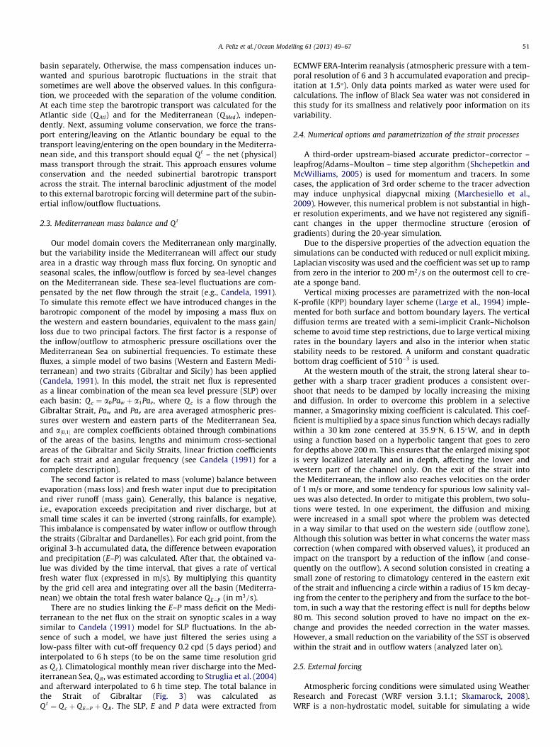
There are no studies linking the E–P mass deficit on the Medi-terranean to the net flux on the strait on synoptic scales in a waysimilar to Candela (1991) model for SLP fluctuations. In the ab-sence of such a model, we have just filtered the series using alow-pass filter with cut-off frequency 0.2 cpd (5 days period) andinterpolated to 6 h steps (to be on the same time resolution gridas Qc). Climatological monthly mean river discharge into the Med-iterranean Sea, Q R, was estimated according to Struglia et al. (2004)and afterward interpolated to 6 h time step. The total balance inthe Strait of Gibraltar (Fig. 3) was calculated asQ t ¼ Qc þ QE—P þ QR. The SLP, E and P data were extracted from

ECMWF ERA-Interim reanalysis (atmospheric pressure with a tem-poral resolution of 6 and 3 h accumulated evaporation and precip-itation at 1.5�). Only data points marked as water were used forcalculations. The inflow of Black Sea water was not considered inthis study for its smallness and relatively poor information on itsvariability.

2.4. Numerical options and parametrization of the strait processes

A third-order upstream-biased accurate predictor–corrector –leapfrog/Adams–Moulton – time step algorithm (Shchepetkin andMcWilliams, 2005) is used for momentum and tracers. In somecases, the application of 3rd order scheme to the tracer advectionmay induce unphysical diapycnal mixing (Marchesiello et al.,2009). However, this numerical problem is not substantial in high-er resolution experiments, and we have not registered any signifi-cant changes in the upper thermocline structure (erosion ofgradients) during the 20-year simulation.

Due to the dispersive properties of the advection equation thesimulations can be conducted with reduced or null explicit mixing.Laplacian viscosity was used and the coefficient was set up to rampfrom zero in the interior to 200 m2=s on the outermost cell to cre-ate a sponge band.

Vertical mixing processes are parametrized with the non-localK-profile (KPP) boundary layer scheme (Large et al., 1994) imple-mented for both surface and bottom boundary layers. The verticaldiffusion terms are treated with a semi-implicit Crank–Nicholsonscheme to avoid time step restrictions, due to large vertical mixingrates in the boundary layers and also in the interior when staticstability needs to be restored. A uniform and constant quadraticbottom drag coefficient of 510�3 is used.

At the western mouth of the strait, the strong lateral shear to-gether with a sharp tracer gradient produces a consistent over-shoot that needs to be damped by locally increasing the mixingand diffusion. In order to overcome this problem in a selectivemanner, a Smagorinsky mixing coefficient is calculated. This coef-ficient is multiplied by a space sinus function which decays radiallywithin a 30 km zone centered at 35:9�N, 6:15�W, and in depthusing a function based on a hyperbolic tangent that goes to zerofor depths above 200 m. This ensures that the enlarged mixing spotis very localized laterally and in depth, affecting the lower andwestern part of the channel only. On the exit of the strait intothe Mediterranean, the inflow also reaches velocities on the orderof 1 m/s or more, and some tendency for spurious low salinity val-ues was also detected. In order to mitigate this problem, two solu-tions were tested. In one experiment, the diffusion and mixingwere increased in a small spot where the problem was detectedin a way similar to that used on the western side (outflow zone).Although this solution was better in what concerns the water masscorrection (when compared with observed values), it produced animpact on the transport by a reduction of the inflow (and conse-quently on the outflow). A second solution consisted in creating asmall zone of restoring to climatology centered in the eastern exitof the strait and influencing a circle within a radius of 15 km decay-ing from the center to the periphery and from the surface to the bot-tom, in such a way that the restoring effect is null for depths below80 m. This second solution proved to have no impact on the ex-change and provides the needed correction in the water masses.However, a small reduction on the variability of the SST is observedwithin the strait and in outflow waters (analyzed later on).

2.5. External forcing

Atmospheric forcing conditions were simulated using WeatherResearch and Forecast (WRF version 3.1.1; Skamarock, 2008).WRF is a non-hydrostatic model, suitable for simulating a wide

−7 −6.5 −6 −5.5 −535.5

35.6

35.7

35.8

35.9

36

36.1

36.2

−6.8 −6.6 −6.4 −6.2 −6 −5.8 −5.6 −5.4 −5.2−1100

−1000

−900

−800

−700

−600

−500

−400

−300

−200

−100

0

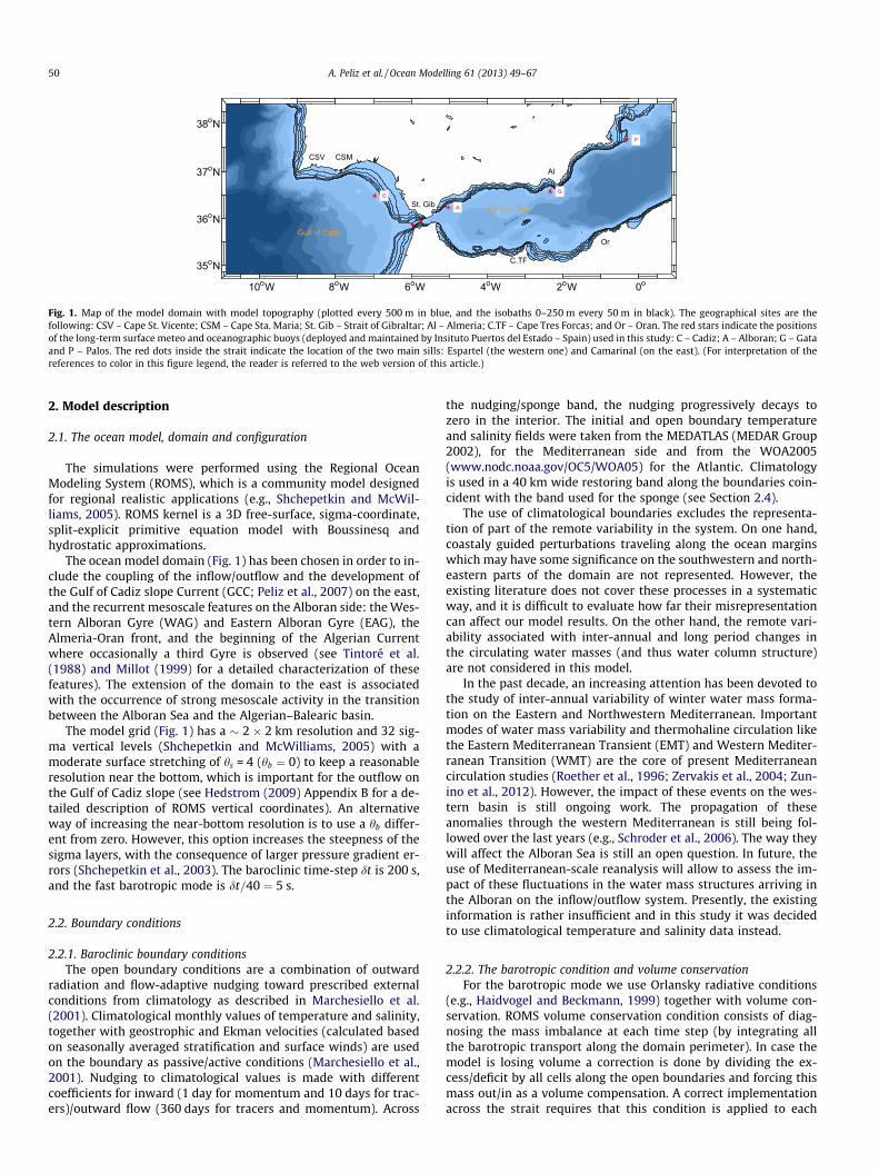
Fig. 2. Top: isobaths 800, 600, 400, 350, 300, 250 and 200 for real (gray) and model(black) topographies in the Strait of Gibraltar zone. The blue/red (real/model) linesshow the channel axis using the maximum depth as a criterium (finding themaximum depth for each topograpic cross-section all along the channel). Bottom:along channel axis depth profile for the model (red) and real data (blue)corresponding to the channel axis lines plotted above. The topography followingmodel layers are represented with thin black lines. (For interpretation of thereferences to color in this figure legend, the reader is referred to the web version ofthis article.)

52 A. Peliz et al. / Ocean Modelling 61 (2013) 49–67

range of scales, from thousands of kilometers to a few meters, witha large number of available options in what concerns the modelcore and most physical parametrizations. In this work, WRF wassetup with two nested grids, one at 27 km and a second at 9 kmhorizontal grid spacing, using one-way nesting. Both grids are cen-

89 90 91 92 93 94 95 96 97 98 9

−0.2

−0.1

0

0.1

0.2

0.3

Mean Qt = 0.057 Sv

Fig. 3. Time series of net flux (Qt) across the Strait of Gibraltar calculated using CandelaQc , evaporation–precipitation (from ERA-Interim data) QE—P and climatological river con

tered in the Iberian Peninsula (IP) and have, respectively,144 � 111 and 162 � 135 grid points, covering the ocean modeldomain shown in Fig. 1. The outermost domain was designed tocover a relatively large ocean area, reducing spurious boundary ef-fects in the inner region. The WRF simulations that we use arethoroughly described and validated from a land-meteorology per-spective in Soares et al. (2012) and Cardoso et al. (2012).

The model is forced by 4-h WRF model outputs at 9 km resolu-tion. Wind stress and air–sea fluxes are calculated internally inROMS using the bulk formulation from Fairall et al. (2003).

Since our goal is to develop a mesoscale model, tidal forcingcould be dispensable in principle. Nevertheless, tides have a greatinfluence on mixing inside the strait, impacting inflowing/outflow-ing water mass characteristics. However, a good representation oftide-driven mixing processes would require much higher resolu-tion and different model physics (Sánchez-Garrido et al., 2011). Be-sides, our strategy to fix the mass flux and to equilibrate theexchanges, depends on the volume conservation between basinsand on the barotropic volume conservation condition, and this isincompatible with the inclusion of tides as a boundary forcing.

2.6. Topography

Two data bases were used: the global (Smith and Sandwell,1997) topography and the local high resolution data described inSanz et al. (1991) that covers in detail the Strait of Gibraltar zone.As in all sigma coordinate models, ROMS requires a significant de-gree of topography smoothing to avoid steep slopes that inducepressure gradient errors (e.g., Shchepetkin et al., 2003). Thissmoothing is usually performed by filtering the initial topography(h) with a logðhÞ based filter (e.g., Penven et al., 2008). The verysteep zones, though, become too smooth after the filter application,since it tends to uplift the deeper parts and make the shallow sidesdeeper. Although the amount of filtering needed strongly dependson the resolution, the very steep slopes are significantly trans-formed even at 2 km, if no additional correction is applied. Fig. 2shows a zoom over the strait topography (gray lines correspondto real topography) where it is possible to observe that the Medi-terranean side of the strait is a steep canyon-like feature. To pre-vent a significant erosion of the strait an iterative procedure wasapplied to this particular location. The filter was designed to con-serve the maximum depth and the cross-channel area of the strait.The resulting topography (black lines in Fig. 2) is smoother, but thedepths of the channel at the main sills and constriction are reason-ably conserved. The lines along the axis of the channel and the sec-tion along them (Fig. 2 bottom) show a good agreement in thenarrow zones of the strait. In the deeper Mediterranean side, how-ever, the match is not as good, but in that case the section is muchdeeper.

9 00 01 02 03 04 05 06 07 08 09

weekly filtered Qt

6−monthly filtered Qt

(1991) for fluctuations associated with Sea Level Pressure inside the Mediterraneantributions QR from Struglia et al. (2004).

−4 −2 0 2 4

Dec

Nov

Oct

Sep

Aug

Jul

Jun

May

Apr

Mar

Feb

Jan Cadiz

m/s−4 −2 0 2 4

Alboran

m/s−4 −2 0 2 4

Gata

m/s−4 −2 0 2 4

Palos

m/s

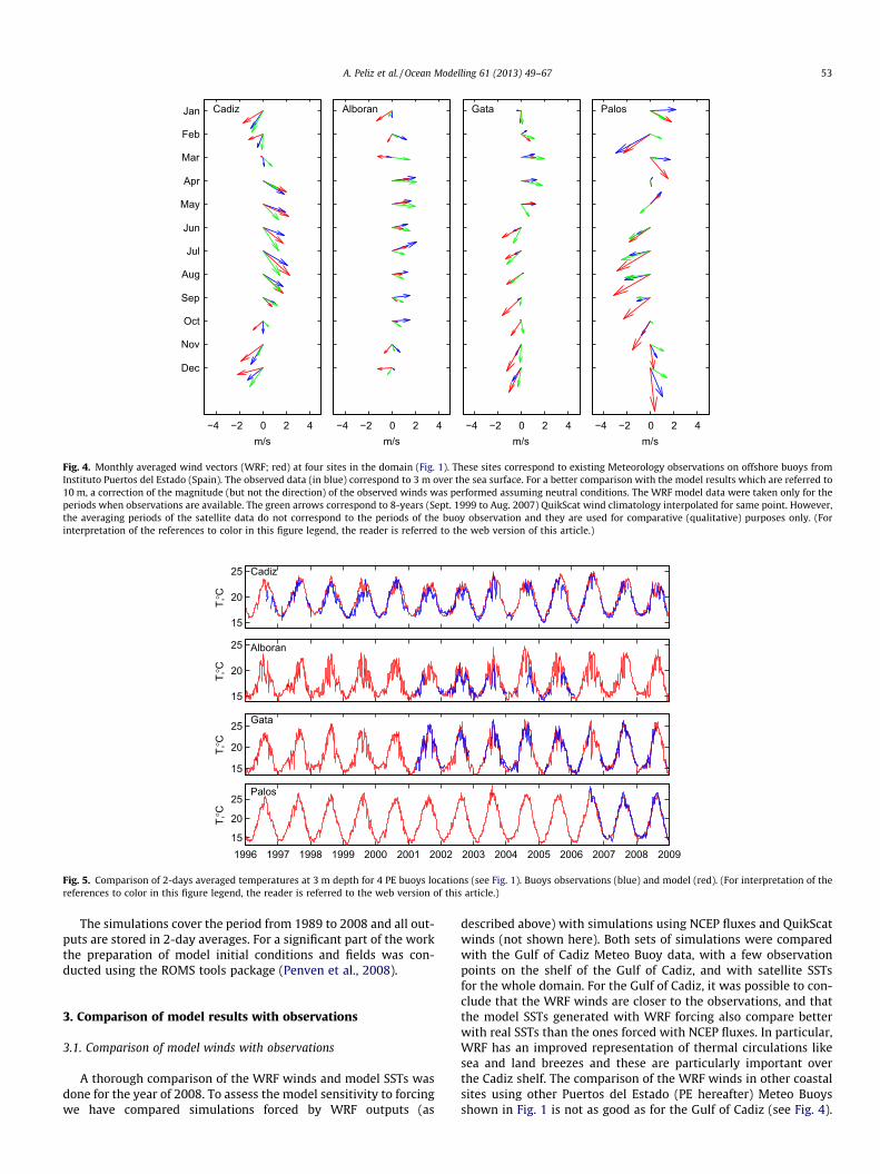
Fig. 4. Monthly averaged wind vectors (WRF; red) at four sites in the domain (Fig. 1). These sites correspond to existing Meteorology observations on offshore buoys fromInstituto Puertos del Estado (Spain). The observed data (in blue) correspond to 3 m over the sea surface. For a better comparison with the model results which are referred to10 m, a correction of the magnitude (but not the direction) of the observed winds was performed assuming neutral conditions. The WRF model data were taken only for theperiods when observations are available. The green arrows correspond to 8-years (Sept. 1999 to Aug. 2007) QuikScat wind climatology interpolated for same point. However,the averaging periods of the satellite data do not correspond to the periods of the buoy observation and they are used for comparative (qualitative) purposes only. (Forinterpretation of the references to color in this figure legend, the reader is referred to the web version of this article.)

15

20

25

T,°C

Cadiz

15

20

25

T,°C

Alboran

15

20

25

T,°C

Gata

1996 1997 1998 1999 2000 2001 2002 2003 2004 2005 2006 2007 2008 200915

20

25

T,°C

Palos

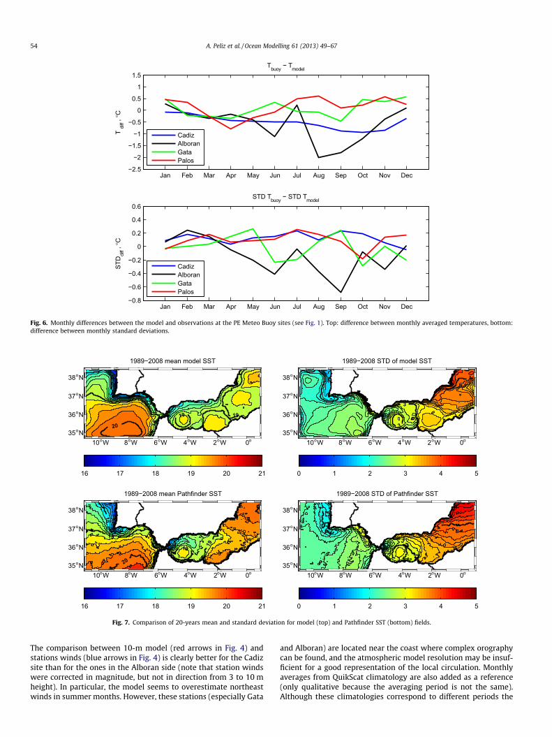
Fig. 5. Comparison of 2-days averaged temperatures at 3 m depth for 4 PE buoys locations (see Fig. 1). Buoys observations (blue) and model (red). (For interpretation of thereferences to color in this figure legend, the reader is referred to the web version of this article.)

A. Peliz et al. / Ocean Modelling 61 (2013) 49–67 53

The simulations cover the period from 1989 to 2008 and all out-puts are stored in 2-day averages. For a significant part of the workthe preparation of model initial conditions and fields was con-ducted using the ROMS tools package (Penven et al., 2008).

3. Comparison of model results with observations

3.1. Comparison of model winds with observations

A thorough comparison of the WRF winds and model SSTs wasdone for the year of 2008. To assess the model sensitivity to forcingwe have compared simulations forced by WRF outputs (as

described above) with simulations using NCEP fluxes and QuikScatwinds (not shown here). Both sets of simulations were comparedwith the Gulf of Cadiz Meteo Buoy data, with a few observationpoints on the shelf of the Gulf of Cadiz, and with satellite SSTsfor the whole domain. For the Gulf of Cadiz, it was possible to con-clude that the WRF winds are closer to the observations, and thatthe model SSTs generated with WRF forcing also compare betterwith real SSTs than the ones forced with NCEP fluxes. In particular,WRF has an improved representation of thermal circulations likesea and land breezes and these are particularly important overthe Cadiz shelf. The comparison of the WRF winds in other coastalsites using other Puertos del Estado (PE hereafter) Meteo Buoysshown in Fig. 1 is not as good as for the Gulf of Cadiz (see Fig. 4).

Jan Feb Mar Apr May Jun Jul Aug Sep Oct Nov Dec−2.5

−2

−1.5

−1

−0.5

0

0.5

1

1.5

Tdi

ff , °C

Tbuoy − Tmodel

CadizAlboranGataPalos

Jan Feb Mar Apr May Jun Jul Aug Sep Oct Nov Dec−0.8

−0.6

−0.4

−0.2

0

0.2

0.4

0.6STD Tbuoy − STD Tmodel

STD

diff ,

°C

CadizAlboranGataPalos

Fig. 6. Monthly differences between the model and observations at the PE Meteo Buoy sites (see Fig. 1). Top: difference between monthly averaged temperatures, bottom:difference between monthly standard deviations.

1718

19

19

19

20

o o o o o o 35oN

36oN

37oN

38oN

1989−2008 mean model SST

16 17 18 19 20 21

22

3 3

3

4

o o o o o 10 W 8 W 6 W 4 W 2 W 0 10 W 8 W 6 W 4 W 2 W 0o 35oN

36oN

37oN

38oN

1989−2008 STD of model SST

0 1 2 3 4 5

1718

19

19

19

20

10oW 8oW 6oW 4oW 2oW 0o 35oN

36oN

37oN

38oN

1989−2008 mean Pathfinder SST

16 17 18 19 20 21

2

2 3

3

3

4

10oW 8oW 6oW 4oW 2oW 0o 35oN

36oN

37oN

38oN

1989−2008 STD of Pathfinder SST

0 1 2 3 4 5

Fig. 7. Comparison of 20-years mean and standard deviation for model (top) and Pathfinder SST (bottom) fields.

54 A. Peliz et al. / Ocean Modelling 61 (2013) 49–67

The comparison between 10-m model (red arrows in Fig. 4) andstations winds (blue arrows in Fig. 4) is clearly better for the Cadizsite than for the ones in the Alboran side (note that station windswere corrected in magnitude, but not in direction from 3 to 10 mheight). In particular, the model seems to overestimate northeastwinds in summer months. However, these stations (especially Gata

and Alboran) are located near the coast where complex orographycan be found, and the atmospheric model resolution may be insuf-ficient for a good representation of the local circulation. Monthlyaverages from QuikScat climatology are also added as a reference(only qualitative because the averaging period is not the same).Although these climatologies correspond to different periods the

25.5 26 26.5 27 27.5 28

0

0.2

0.4

0.6

0.8

1

1.2

1.4

(a) Average dens. anomaly

29.929.428.928.427.927.4

26.9

26.4

25.9

25.4

24.9

24.4

23.9

23.4

(b) TS diagram

35 36 37 38

10

15

20

25 BP−StGib1989clm

10 12 14 16 18 20 22

25.5

26

26.5

27

27.5

28

28.5

29

29.5

temp.

σ−t

(c)

35 36 37 38 39

25.5

26

26.5

27

27.5

28

28.5

29

29.5

salt.

θ

(d)

26 27 28 29 30

0.05

0.1

0.15

0.2

0.25

0.3

0.35

0.4

0.45

0.5

0.55

(a) Average dens. anomaly

2928.52827.527

26.5

26

25.5

25

24.5

24

23.5

23

22.5

(b) TS diagram

35.5 36 36.5 37 37.5 38 38.5

12

14

16

18

20

22

24

26

28 Alboran−c2903453−9921992clm

12 14 16 18 20 22

25.5

26

26.5

27

27.5

28

28.5

29

29.5

temp.

σ−t

(c)

36 36.5 37 37.5 38 38.5

25.5

26

26.5

27

27.5

28

28.5

29

29.5

salt.

θ

(d)

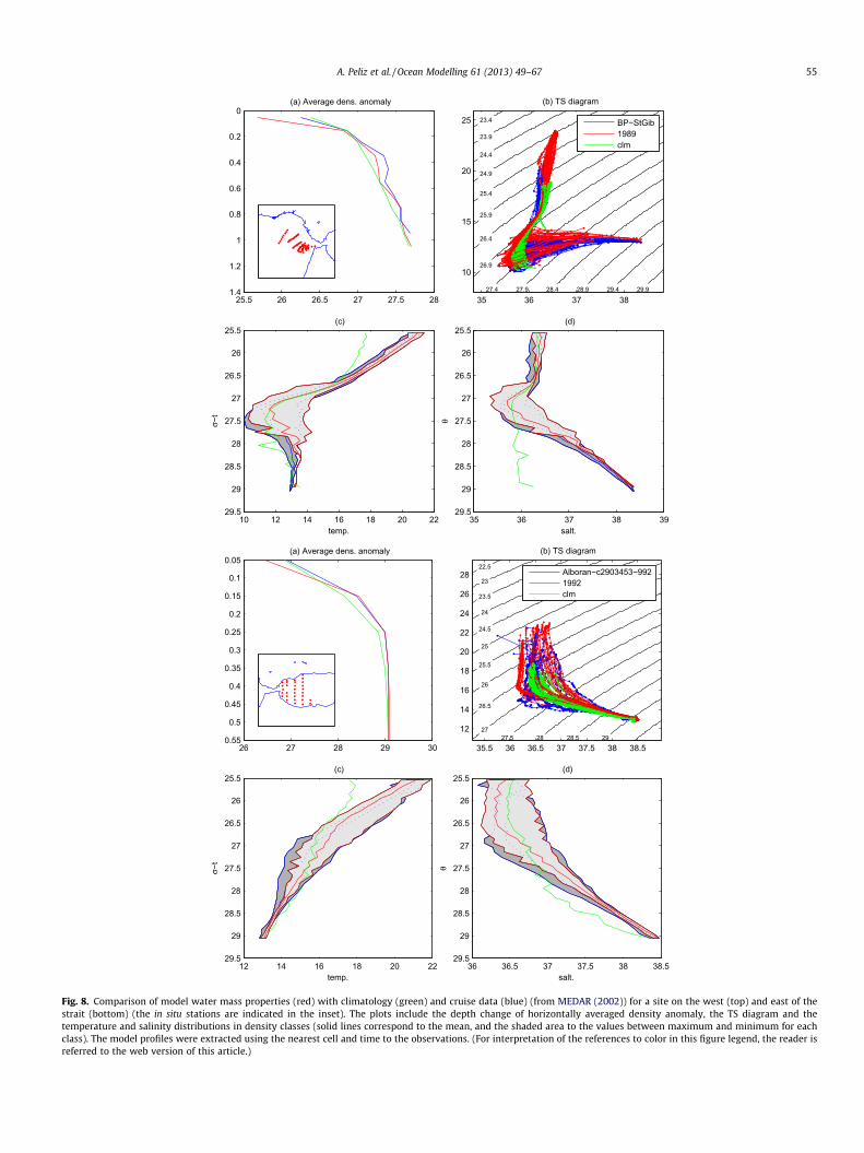
Fig. 8. Comparison of model water mass properties (red) with climatology (green) and cruise data (blue) (from MEDAR (2002)) for a site on the west (top) and east of thestrait (bottom) (the in situ stations are indicated in the inset). The plots include the depth change of horizontally averaged density anomaly, the TS diagram and thetemperature and salinity distributions in density classes (solid lines correspond to the mean, and the shaded area to the values between maximum and minimum for eachclass). The model profiles were extracted using the nearest cell and time to the observations. (For interpretation of the references to color in this figure legend, the reader isreferred to the web version of this article.)

A. Peliz et al. / Ocean Modelling 61 (2013) 49–67 55

56 A. Peliz et al. / Ocean Modelling 61 (2013) 49–67

comparison with satellite winds confirm that the agreement in theGulf of Cadiz side is better, and that WRF northeast winds are toostrong in the northeast part of the domain.

3.2. Comparison of model surface temperature with observations

Model and in situ (from PE meteo buoys) temperatures at 3 mdepth show a good agreement (Fig. 5). The model responds to sea-sonal, inter-annual and to most of the synoptic fluctuations with agreat detail. The seasonal amplitude is of about of 8—9 �C for theCadiz and Alboran sites and above 10 �C for the Gata and Palos re-gions. The upper plot in Fig. 6 compares the differences in seasonalcycle between observed and model temperatures. For the Gulf ofCadiz Buoy, model temperatures are slightly warmer than ob-served over all the months, with annual mean temperature differ-ence of about 0:5 �C (maximum of 1 �C in October). For the AlboranBuoy, the annual mean temperature difference is similar to that ofthe Cadiz site �0:6 �C (model is warmer than observations), but inthe annual cycle these differences are higher with maximumvalues observed in August of about 2 �C. For the Gata and PalosBuoys, annual mean temperature differences are of about 0:1 �C,but contrary to Cadiz and Alboran, these zones are colder in themodel.

For what concerns the annual cycle, the differences in standarddeviations (bottom plot of Fig. 6), in general, do not exceed 0:2 �Cfor Cadiz, Gata and Palos sites. For the Alboran Buoy this differencereaches 0:7 �C in September (model STD higher than observed).This can be explained by the proximity of this site to the northernedge of the Atlantic jet and all the variability associated with thejet meridional excursions.

In Fig. 7, a comparison between 20-year average and corre-sponding standard deviations of the model and Pathfinder SSTs isshown. In general, the model and Pathfinder SST data show a good

Alboran−c2903453−992 Sep92

S 100m

−5 −4 −3 −2 −1 035

35.5

36

36.5

37

37.536 36.5 37 37.5 38

roms 1992

S 100m

−5 −4 −3 −2 −1 035

35.5

36

36.5

37

37.536 36.5 37 37.5 38

Alboran−c2903453−992 Sep92

θ 100m

−5 −4 −3 −2 −1 035

35.5

36

36.5

37

37.513 14 15 16 17 18 19 20 21

θ 100m

roms 1992

−5 −4 −3 −2 −1 035

35.5

36

36.5

37

37.513 14 15 16 17 18 19 20 21

Alboran−c2903453−992 Sep92

σθ 100m

−5 −4 −3 −2 −1 035

35.5

36

36.5

37

37.526 26.5 27 27.5 28 28.5

σθ 100m

roms 1992

−5 −4 −3 −2 −1 035

35.5

36

36.5

37

37.526 26.5 27 27.5 28 28.5

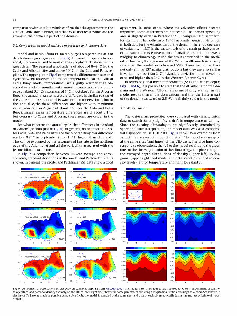
Fig. 9. Comparison of observations (cruise Alboran-c2903453 Sept. 92 from MEDAR (20temperature, and potential density anomaly on the 100 m level; right side, shows the sathe inset). To have as much as possible comparable fields, the model is sampled at theoutput).

agreement. In some zones where the advective effects becomeimportant, some differences are noticeable. The Iberian upwellingarea is slightly wider in Pathfinder SST (compare 18 �C isotherm,for example). The isotherm of 19 �C has similar spatial distributionin both data for the Atlantic part of the domain. There is a decreaseof variability in SST in the eastern exit of the strait probably asso-ciated with the misrepresentation of small scales and to the weaknudging to climatology inside the strait (described in the meth-ods). However, the signature of the Western Alboran Gyre is verysimilar in the model and observed SSTs. These two zones havenot only similar SST spatial distributions but they are also similarin variability (less than 2 �C of standard deviation in the upwellingzone and higher than 3 �C in the Western Alboran Gyre).

In terms of global mean temperatures (SSTs and at 3 m depth;Figs. 7 and 6), it is possible to state that the Atlantic part of the do-main and the Western Alboran areas are slightly warmer in themodel results than in the observations, and that the Eastern partof the domain (eastward of 2:5 �W) is slightly colder in the model.

3.3. Water masses

The water mass properties were compared with climatologicaldata to search for any significant drift in temperature or salinity.Since the existing climatologies are significantly smoothed byspace and time interpolation, the model data was also comparedwith synoptic cruise CTD data. Fig. 8 shows two examples fromsynoptic cruises on both sides of the strait. The model was sampledat the same sites (and times) of the CTD casts. The blue lines cor-respond to observations, the red to the model results and the greenones to the closest grid point of the climatology. The plots comparethe averaged depth distributions of density (upper left), TS dia-grams (upper right) and model and data statistics binned in den-sity levels (left for temperature and right for salinity).

−5 −4 −3 −2 −1−400

−350

−300

−250

−200

−150

−100

−50

035.5 36 36.5 37 37.5 38

−5 −4 −3 −2 −1−400

−350

−300

−250

−200

−150

−100

−50

035.5 36 36.5 37 37.5 38

−5 −4 −3 −2 −1−400

−350

−300

−250

−200

−150

−100

−50

012 14 16 18 20 22

−5 −4 −3 −2 −1−400

−350

−300

−250

−200

−150

−100

−50

012 14 16 18 20 22

−5 −4 −3 −2 −1−400

−350

−300

−250

−200

−150

−100

−50

024.5 25.5 26.5 27.5 28.5

−5 −4 −3 −2 −1−400

−350

−300

−250

−200

−150

−100

−50

024.5 25.5 26.5 27.5 28.5

02)) and model internal structure: left side (top to bottom) shows fields of salinity,me parameters but along a longitudinal section crossing the Alboran Sea (shown insame sites and date of each observed profile (using the nearest cell/time of model

A. Peliz et al. / Ocean Modelling 61 (2013) 49–67 57

On the western side, there is a good match between observedand model temperatures and salinities at almost all levels. Notethat the model drifts from the climatological values (which corre-spond to the initialization values as well) and adjusts to those ofthe observations. A small difference on higher density levels pointsout towards a slightly warmer and saltier outflow which is how-ever density compensated. The very complex mixing mechanismsin the strait are marginally represented even at the present resolu-tion. The method which was adopted to increase mixing in thestrait produces good results in what concerns the product outflowwater mass. On the surface levels of the Alboran Side (the lower setof plots in Fig. 8), a small tendency for fresher/colder waters on thelevels above 27 rt is observed, but the difference is not very signif-icant. It is possible to say that the Atlantic Water inside the Alboranis being represented within a good range of variability. A small biasof the subsurface minimum towards fresher and warmer values isnoticeable.

3.4. Internal structure

The internal structure of the model is compared with synopticcruise data in Fig. 9. The Alboran Sea jets and gyres are the mainfeatures of the western part of the Basin and the model skill toaccurately represent these flow structures is critical. The left panelsof the plot compare model and observed fields at 100 m depth. Onthe right side, we show data along a section from the same survey(note that the model was sub-sampled at the sites and times of theCTD casts before reproducing the model fields). The comparisonshows that the Atlantic jet and both gyres are represented (for a

0 0.2 0.4 0.6 0.8 1 1.2

−300

−250

−200

−150

−100

−50

0(a) Espartel sill

[m/s]

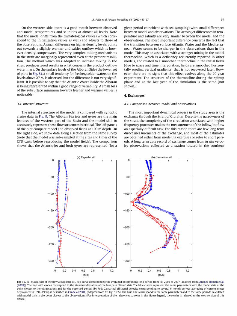
Fig. 10. (a) Magnitude of the flow at Espartel sill. Red curve correspond to the averaged o(2009)). The line with circles correspond to the standard deviation of the low pass filterpoint closest to the observations and for the observed period. (b) Red: Camarinal sill zodeployments (1994–1996) as described in Candela (2001) (adapted from his Fig. 5.7.5). Twith model data in the point closest to the observations. (For interpretation of the referarticle.)

given period coincident with sea sampling) with small differencesbetween model and observations. The across jet differences in tem-perature and salinity are very similar between the model and theobservations. The most important difference concerns the fact thatthe transition between surface Atlantic Water and the Mediterra-nean Water seems to be sharper in the observations than in themodel. This may be associated with a stronger mixing in the modelthermocline, which is a deficiency recurrently reported in othermodels, and related to a smoothed thermocline in the initial fields(due to space and time interpolation, fields are smoothed horizon-tally eroding vertical gradients) that is not recovered later. How-ever, there are no signs that this effect evolves along the 20-yearexperiment. The structure of the thermocline during the spinupphase and at the last year of the simulation is the same (notshown).

4. Exchanges

4.1. Comparison between model and observations

The most important dynamical process in the study area is theexchange through the Strait of Gibraltar. Despite the narrowness ofthe strait, the complexity of the circulation associated with higherfrequency processes makes the measurement of the inflow/outflowan especially difficult task. For this reason there are few long termdirect measurements of the exchange, and most of the estimatesare obtained either from modeling exercises or refer to short peri-ods. A long term data record of exchange comes from in situ veloc-ity observations collected at a station located in the southern

0 0.2 0.4 0.6 0.8 1 1.2

−300

−250

−200

−150

−100

−50

0(b) Camarinal sill

[m/s]

bservations for a period from fall 2004 to 2007 (adapted from Sánchez-Román et al.ed data The blue curves represent the same parameters with the model data at thenal velocity corresponding to several 6-month periods averaging of current meter

he blue lines correspond to the same parameters and to the same periods calculatedences to color in this figure legend, the reader is referred to the web version of this

58 A. Peliz et al. / Ocean Modelling 61 (2013) 49–67

channel of the Espartel sill, at the western exit of the strait (35�

51.700 N, 5� 58.600 W at 360 m depth; western red dot in Fig. 1)in the framework of the Spanish funded INGRES I, II and III projects.This station is equipped with an up-looking ADCP settled 15 mabove the seafloor, a point-wise current meter and an autonomousconductivity-temperature probe at 8 and 5 m above the seafloor,respectively. Using these current velocity data (Sánchez-Románet al., 2009) estimated the outflow through the Strait of Gibraltarfrom October 2004 (first data acquired) to January 2009. Anotherset of exchange flow data is described in Candela (2001), and orig-inates from near 2 years (1994–1996) of current meter measure-ments (single point and profilers) collected over the Camarinalsill (eastern red dot in the strait in Fig. 1).

2005 2006

−1.1

−1

−0.9

−0.8

−0.7

−0.6

−0.5

−0.4(a) Qo time series (w

Model Qom = −0.771 ± 0.

Obser Qoo = −0.771 ± 0.0

2005 20060.6

0.7

0.8

0.9

1

1.1(b) Qi time serie

Qio = 0.813 ± 0.056

Qim = 0.834 ± 0.051

2005 20060

5

10

15

20

25

30 (c) |Q

m−Q

o|

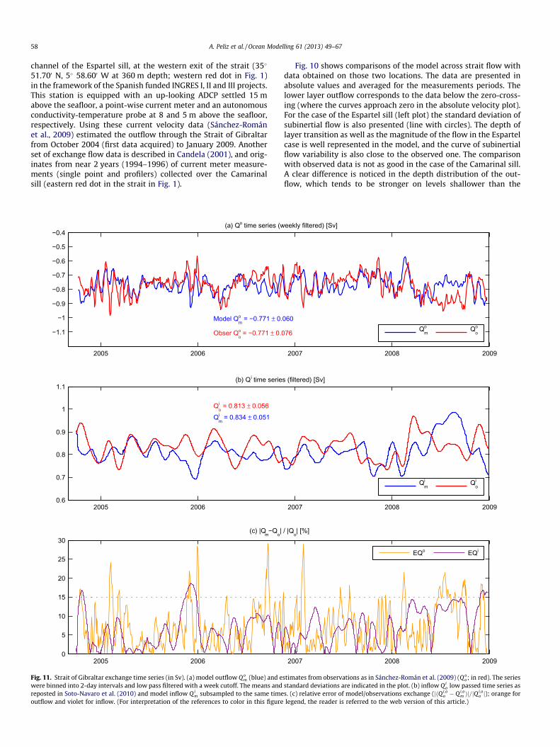
Fig. 11. Strait of Gibraltar exchange time series (in Sv). (a) model outflow Qom (blue) and e

were binned into 2-day intervals and low pass filtered with a week cutoff. The means andreposted in Soto-Navaro et al. (2010) and model inflow Qi

m subsampled to the same timeoutflow and violet for inflow. (For interpretation of the references to color in this figure

Fig. 10 shows comparisons of the model across strait flow withdata obtained on those two locations. The data are presented inabsolute values and averaged for the measurements periods. Thelower layer outflow corresponds to the data below the zero-cross-ing (where the curves approach zero in the absolute velocity plot).For the case of the Espartel sill (left plot) the standard deviation ofsubinertial flow is also presented (line with circles). The depth oflayer transition as well as the magnitude of the flow in the Espartelcase is well represented in the model, and the curve of subinertialflow variability is also close to the observed one. The comparisonwith observed data is not as good in the case of the Camarinal sill.A clear difference is noticed in the depth distribution of the out-flow, which tends to be stronger on levels shallower than the

2007 2008 2009

eekly filtered) [Sv]

060

76 Qom

Qoo

2007 2008 2009

s (filtered) [Sv]

Qim

Qio

2007 2008 2009

/ |Qo| [%]

EQo EQi

stimates from observations as in Sánchez-Román et al. (2009) (Qoo; in red). The series

standard deviations are indicated in the plot. (b) inflow Qio low passed time series as

s. (c) relative error of model/observations exchange (jðQi;oo � Qi;o

m Þj=jQi;oo j); orange for

legend, the reader is referred to the web version of this article.)

A. Peliz et al. / Ocean Modelling 61 (2013) 49–67 59

observations where the outflow seems to be already bottomtrapped, or at least to have its maximum at a deeper level. Con-versely, the deeper levels of the inflow seem to be stronger inthe model than in the observations. This difference in the verticalstructure (more smoothed in the observations and more shearedin the model) may be associated with the lack of higher frequencydynamics in the model and consequent misrepresentation of themixing processes. Nevertheless, the magnitude and variability ofthe inflow and of the outflow seem to be in agreement with theobservations and we next analyse these two quantities in inte-grated terms (exchange).

Since our model excludes high frequency tidal variability, wecompare the model-observation outflow estimate (Qo

o) in thesub-inertial range (the analysis is restricted to the Espartel dataonly). At weekly to monthly scales (see Fig. 11), the model followsthe observations rather well (note that statistics are practicallyidentical) with almost all events being captured by the model,although sometimes the observations seem to show fluctuationsof larger amplitude (e.g., the winter of 2005). On the seasonal scale,the mean outflow value also follows the one obtained from theobservations rather well, with only a few periods when diver-gences in the order of 0.05 Sv are observed between both series(summers 2006 and 2008). In fact, the larger deviations occur insummer with a tendency for the model to have an outflow strongerthan the one estimated from observations, with the exception of2008 when the opposite is observed. During the remaining partof the year the differences between model and observations arenot relevant, and the relative error rarely exceeds the 15% thresh-old (see Fig. 11c).

There is no direct estimate of inflow from observations (Qio)

since Espartel observations miss the bulk of the upper layer. How-ever, Soto-Navaro et al. (2010) computed this variable by combin-ing the outflow data with estimates of the Mediterranean massbudget. The comparison between our estimate and that of Soto-Navaro et al. (2010) is thus of relative validity and should be inter-preted with caution. Fig. 11b shows only the low frequency esti-mates presented in Soto-Navaro et al. (2010), together withmodel estimate filtered in the same manner. The statistics are close(Q i

o ¼ 0:813� 0:056Sv; Q im ¼ 0:834� 0:051Sv) and the two esti-

mates are several times in phase, but the comparison is clearly

Perio

d

(a) Qoo

05 06 07

4 8 16 32 64128256512

Perio

d

(b) Qom

05 06 07

4 8 16 32 64128256512

Fig. 12. Wavelet of outflow estimated from observations (a) and model (b). The y-aximeasurements period (2004–2008). Colors show the relative energy spectral density on

not as good as for the outflow. Nevertheless the relative error issmall (Fig. 11c; violet line).

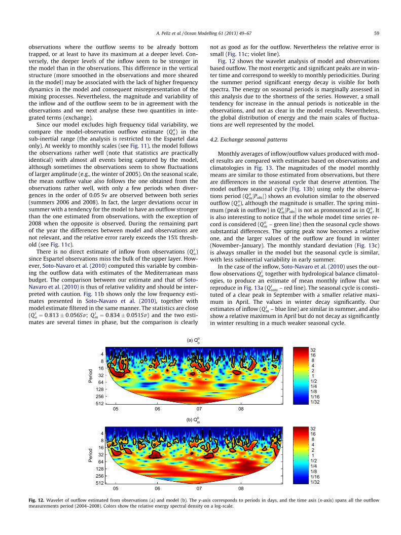
Fig. 12 shows the wavelet analysis of model and observationsbased outflow. The most energetic and significant peaks are in win-ter time and correspond to weekly to monthly periodicities. Duringthe summer period significant energy decay is visible for bothspectra. The energy on seasonal periods is marginally assessed inthis analysis due to the shortness of the series. However, a smalltendency for increase in the annual periods is noticeable in theobservations, and not as clear in the model results. Nevertheless,the global distribution of energy and the main scales of fluctua-tions are well represented by the model.

4.2. Exchange seasonal patterns

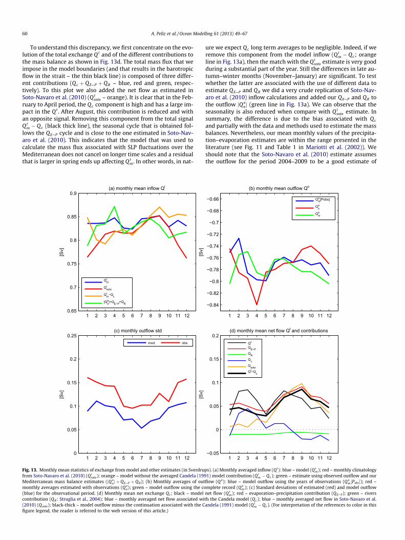
Monthly averages of inflow/outflow values produced with mod-el results are compared with estimates based on observations andclimatologies in Fig. 13. The magnitudes of the model monthlymeans are similar to those estimated from observations, but thereare differences in the seasonal cycle that deserve attention. Themodel outflow seasonal cycle (Fig. 13b) using only the observa-tions period (Q o

m½Pobs�) shows an evolution similar to the observedoutflow (Q o

o), although the magnitude is smaller. The spring mini-mum (peak in outflow) in Q o

m½Pobs� is not as pronounced as in Q oo. It

is also interesting to notice that if the whole model time series re-cord is considered (Qo

m – green line) then the seasonal cycle showssubstantial differences. The spring peak now becomes a relativeone, and the larger values of the outflow are found in winter(November–January). The monthly standard deviation (Fig. 13c)is always smaller in the model but the seasonal cycle is similar,with less subinertial variability in early summer.

In the case of the inflow, Soto-Navaro et al. (2010) uses the out-flow observations Qi

o together with hydrological balance climatol-ogies, to produce an estimate of mean monthly inflow that wereproduce in Fig. 13a (Qi

soto – red line). The seasonal cycle is consti-tuted of a clear peak in September with a smaller relative maxi-mum in April. The values in winter decay significantly. Ourestimates of inflow (Q i

m – blue line) are similar in summer, and alsoshow a relative maximum in April but do not decay as significantlyin winter resulting in a much weaker seasonal cycle.

081/321/161/81/41/2 1 2 4 81632

081/321/161/81/41/2 1 2 4 81632

s corresponds to periods in days, and the time axis (x-axis) spans all the outflowa log-scale.

60 A. Peliz et al. / Ocean Modelling 61 (2013) 49–67

To understand this discrepancy, we first concentrate on the evo-lution of the total exchange Q t and of the different contributions tothe mass balance as shown in Fig. 13d. The total mass flux that weimpose in the model boundaries (and that results in the barotropicflow in the strait – the thin black line) is composed of three differ-ent contributions (Q c þ QE—P þ QR – blue, red and green, respec-tively). To this plot we also added the net flow as estimated inSoto-Navaro et al. (2010) (Qt

soto – orange). It is clear that in the Feb-ruary to April period, the Q c component is high and has a large im-pact in the Qt . After August, this contribution is reduced and withan opposite signal. Removing this component from the total signalQt

m � Q c (black thick line), the seasonal cycle that is obtained fol-lows the QE—P cycle and is close to the one estimated in Soto-Nav-aro et al. (2010). This indicates that the model that was used tocalculate the mass flux associated with SLP fluctuations over theMediterranean does not cancel on longer time scales and a residualthat is larger in spring ends up affecting Qt

m. In other words, in nat-

1 2 3 4 5 6 7 8 9 10 11 120.65

0.7

0.75

0.8

0.85

0.9

[Sv]

(a) monthly mean inflow Qi

Qim

Qisoto

Qim−Qc

|Qoo|+QE−P+QR

[Sv]

1 2 3 4 5 6 7 8 9 10 11 120

0.05

0.1

0.15

0.2

0.25

[Sv]

(c) monthly outflow std

mod. obs.

[Sv]

Fig. 13. Monthly mean statistics of exchange from model and other estimates (in Sverdrufrom Soto-Navaro et al. (2010) (Qi

soto); orange – model without the averaged Candela (19Mediterranean mass balance estimates (jQo

oj þ QE—P þ QR); (b) Monthly averages of outmonthly averages estimated with observations (Qo

o); green – model outflow using the c(blue) for the observational period. (d) Monthly mean net exchange Qt; black – modelcontribution (QR: Struglia et al., 2004); blue – monthly averaged net flow associated wi(2010) (Qsoto); black-thick – model outflow minus the continuation associated with the Cfigure legend, the reader is referred to the web version of this article.)

ure we expect Qc long term averages to be negligible. Indeed, if weremove this component from the model inflow (Q i

m � Qc; orangeline in Fig. 13a), then the match with the Qi

soto estimate is very goodduring a substantial part of the year. Still the differences in late au-tumn–winter months (November–January) are significant. To testwhether the latter are associated with the use of different data toestimate Q E—P and Q R we did a very crude replication of Soto-Nav-aro et al. (2010) inflow calculations and added our Q E—P and QR tothe outflow jQ o

oj (green line in Fig. 13a). We can observe that theseasonality is also reduced when compare with Q i

soto estimate. Insummary, the difference is due to the bias associated with Qc

and partially with the data and methods used to estimate the massbalances. Nevertheless, our mean monthly values of the precipita-tion–evaporation estimates are within the range presented in theliterature (see Fig. 11 and Table 1 in Mariotti et al. (2002)). Weshould note that the Soto-Navaro et al. (2010) estimate assumesthe outflow for the period 2004–2009 to be a good estimate of

1 2 3 4 5 6 7 8 9 10 11 12

−0.84

−0.82

−0.8

−0.78

−0.76

−0.74

−0.72

−0.7

−0.68

−0.66

(b) monthly mean outflow Qo

Qom[Pobs]

Qoo

Qom

1 2 3 4 5 6 7 8 9 10 11 12−0.05

0

0.05

0.1

0.15

0.2(d) monthly mean net flow Qt and contributions

Qt

QE−PQRQcQsotoQt−Qc

ps). (a) Monthly averaged inflow (Qi): blue – model (Qim); red – monthly climatology

91) model contribution (Qim � Qc); green – estimate using observed outflow and our

flow (Qo): blue – model outflow using the years of observations (Qom½Pobs�); red –

omplete record (Qom); (c) Standard deviations of estimated (red) and model outflow

net flow (Qtm); red – evaporation–precipitation contribution (QE—P); green – rivers

th the Candela model (Qc); blue – monthly averaged net flow in Soto-Navaro et al.andela (1991) model (Qt

m � Qc). (For interpretation of the references to color in this

A. Peliz et al. / Ocean Modelling 61 (2013) 49–67 61

the climatological values. However we see substantial differencesbetween the outflow monthly climatology considering only theseyears and the climatology based on the 20-year period (comparethe green and blue lines in Fig. 13b). The differences are preciselyduring the months when our estimates diverge (in winter).

5. Mean circulation and seasonal cycle

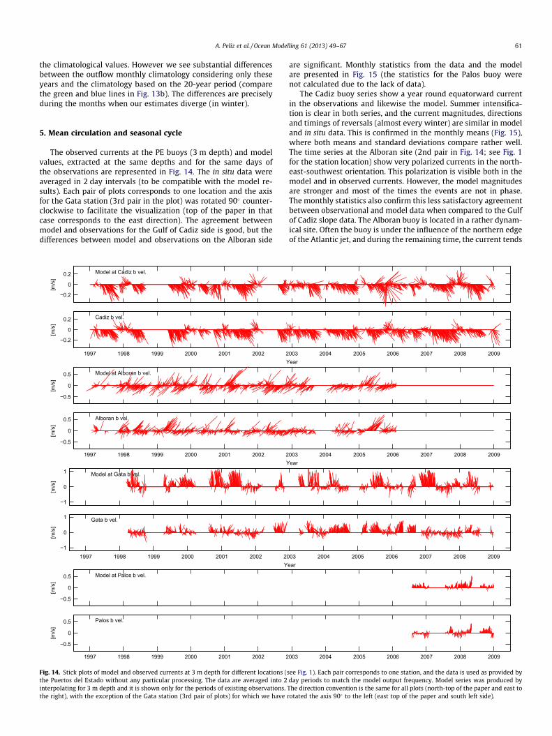
The observed currents at the PE buoys (3 m depth) and modelvalues, extracted at the same depths and for the same days ofthe observations are represented in Fig. 14. The in situ data wereaveraged in 2 day intervals (to be compatible with the model re-sults). Each pair of plots corresponds to one location and the axisfor the Gata station (3rd pair in the plot) was rotated 90� counter-clockwise to facilitate the visualization (top of the paper in thatcase corresponds to the east direction). The agreement betweenmodel and observations for the Gulf of Cadiz side is good, but thedifferences between model and observations on the Alboran side

1997 1998 1999 2000 2001 2002 2

−0.2

0

0.2

Y

[m/s

]

Cadiz b vel.

−0.2

0

0.2

[m/s

]

Model at Cadiz b vel.

1997 1998 1999 2000 2001 2002 2

−0.5

0

0.5

Y

[m/s

]

Alboran b vel.

−0.5

0

0.5

[m/s

]

Model at Alboran b vel.

1997 1998 1999 2000 2001 2002 20−1

0

1

Y

[m/s

]

Gata b vel.

−1

0

1

[m/s

]

Model at Gata b vel.

1997 1998 1999 2000 2001 2002 2

−0.5

0

0.5

[m/s

]

Palos b vel.

−0.5

0

0.5

[m/s

]

Model at Palos b vel.

Fig. 14. Stick plots of model and observed currents at 3 m depth for different locations (sthe Puertos del Estado without any particular processing. The data are averaged into 2interpolating for 3 m depth and it is shown only for the periods of existing observations.the right), with the exception of the Gata station (3rd pair of plots) for which we have

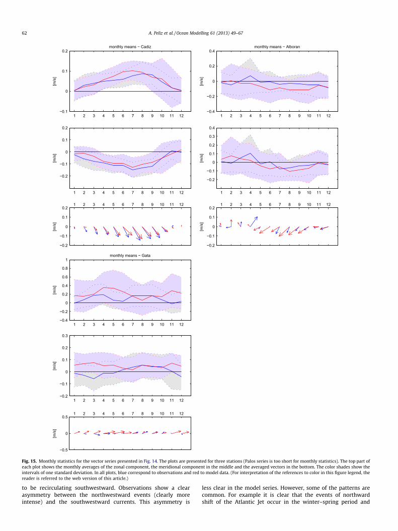
are significant. Monthly statistics from the data and the modelare presented in Fig. 15 (the statistics for the Palos buoy werenot calculated due to the lack of data).

The Cadiz buoy series show a year round equatorward currentin the observations and likewise the model. Summer intensifica-tion is clear in both series, and the current magnitudes, directionsand timings of reversals (almost every winter) are similar in modeland in situ data. This is confirmed in the monthly means (Fig. 15),where both means and standard deviations compare rather well.The time series at the Alboran site (2nd pair in Fig. 14; see Fig. 1for the station location) show very polarized currents in the north-east-southwest orientation. This polarization is visible both in themodel and in observed currents. However, the model magnitudesare stronger and most of the times the events are not in phase.The monthly statistics also confirm this less satisfactory agreementbetween observational and model data when compared to the Gulfof Cadiz slope data. The Alboran buoy is located in a rather dynam-ical site. Often the buoy is under the influence of the northern edgeof the Atlantic jet, and during the remaining time, the current tends

003 2004 2005 2006 2007 2008 2009ear

003 2004 2005 2006 2007 2008 2009ear

03 2004 2005 2006 2007 2008 2009ear

003 2004 2005 2006 2007 2008 2009

ee Fig. 1). Each pair corresponds to one station, and the data is used as provided byday periods to match the model output frequency. Model series was produced by

The direction convention is the same for all plots (north-top of the paper and east torotated the axis 90� to the left (east top of the paper and south left side).

1 2 3 4 5 6 7 8 9 10 11 12−0.1

0

0.1

0.2[m

/s]

monthly means − Cadiz

1 2 3 4 5 6 7 8 9 10 11 12

−0.2

−0.1

0

0.1

0.2

[m/s

]

1 2 3 4 5 6 7 8 9 10 11 12

−0.2

−0.1

0

0.1

0.2

[m/s

]

1 2 3 4 5 6 7 8 9 10 11 12−0.4

−0.2

0

0.2

0.4

[m/s

]

monthly means − Alboran

1 2 3 4 5 6 7 8 9 10 11 12

−0.2

−0.1

0

0.1

0.2

0.3

0.4

[m/s

]1 2 3 4 5 6 7 8 9 10 11 12

−0.2

−0.1

0

0.1

0.2

[m/s

]

1 2 3 4 5 6 7 8 9 10 11 12−0.4

−0.2

0

0.2

0.4

0.6

0.8

1

[m/s

]

monthly means − Gata

1 2 3 4 5 6 7 8 9 10 11 12−0.2

−0.1

0

0.1

0.2

0.3

[m/s

]

1 2 3 4 5 6 7 8 9 10 11 12

−0.5

0

0.5

[m/s

]

Fig. 15. Monthly statistics for the vector series presented in Fig. 14. The plots are presented for three stations (Palos series is too short for monthly statistics). The top part ofeach plot shows the monthly averages of the zonal component, the meridional component in the middle and the averaged vectors in the bottom. The color shades show theintervals of one standard deviation. In all plots, blue correspond to observations and red to model data. (For interpretation of the references to color in this figure legend, thereader is referred to the web version of this article.)

62 A. Peliz et al. / Ocean Modelling 61 (2013) 49–67

to be recirculating southwestward. Observations show a clearasymmetry between the northwestward events (clearly moreintense) and the southwestward currents. This asymmetry is

less clear in the model series. However, some of the patterns arecommon. For example it is clear that the events of northwardshift of the Atlantic Jet occur in the winter–spring period and

1 2 3

4 5 6

7 8 9

10 11 12

0 0.2 0.4 0.6 0.8

1 2 3

4 5 6

7 8 9

10 11 12

0 0.05 0.1 0.15 0.2 0.25 0.3 0.35

Fig. 16. Monthly mean circulation at 30 m depth for the Gulf of Cadiz. The vectors are plotted every eight cells. Colors represent the averaged current magnitude. The starsshow the locations of observed time series (PE meteo buoys). (For interpretation of the references to color in this figure legend, the reader is referred to the web version of thisarticle.)

A. Peliz et al. / Ocean Modelling 61 (2013) 49–67 63

some of them are simulated in phase (1999, 2001, 2002 and2005).

The Gata buoy is also placed in a variable and complex site. Themooring is positioned off the slope in a small bay between twopromontories (see Fig. 1) prone to separation events of slope cur-rents from any of the directions. Nevertheless, it is clear that thedominant direction is eastward (note that east is to the top of the

paper for the Gata station; Fig. 14, 3rd pair). The clearest differencesbetween model and observations concern larger magnitude andpersistence of the eastward currents in the model when comparedwith observations. The phase presents also strong variability reveal-ing reasonable agreement between 2002 and 2007, but with cleardifferences in the other period. There is no obvious seasonal pattern,both in model and observations, and the monthly statistics (Fig. 15)

64 A. Peliz et al. / Ocean Modelling 61 (2013) 49–67

do not disclose any other interesting feature in that respect. The dif-ferences between the model and the observations are more likelyassociated with the turbulent nature of the flow rather than withany systematic tendency of the model. Nevertheless, the modeltends to overestimate the episodes of eastward flow at that site.The vectors series for Palos station are also presented, but theyare too short to support any reliable analysis of monthly statistics.

1

4

7

10

4.02.00

Fig. 17. Monthly mean circulation at 30 m depth for the Alboran Sea. The vectors are plshow the locations of observed time series (PE meteo buoys).

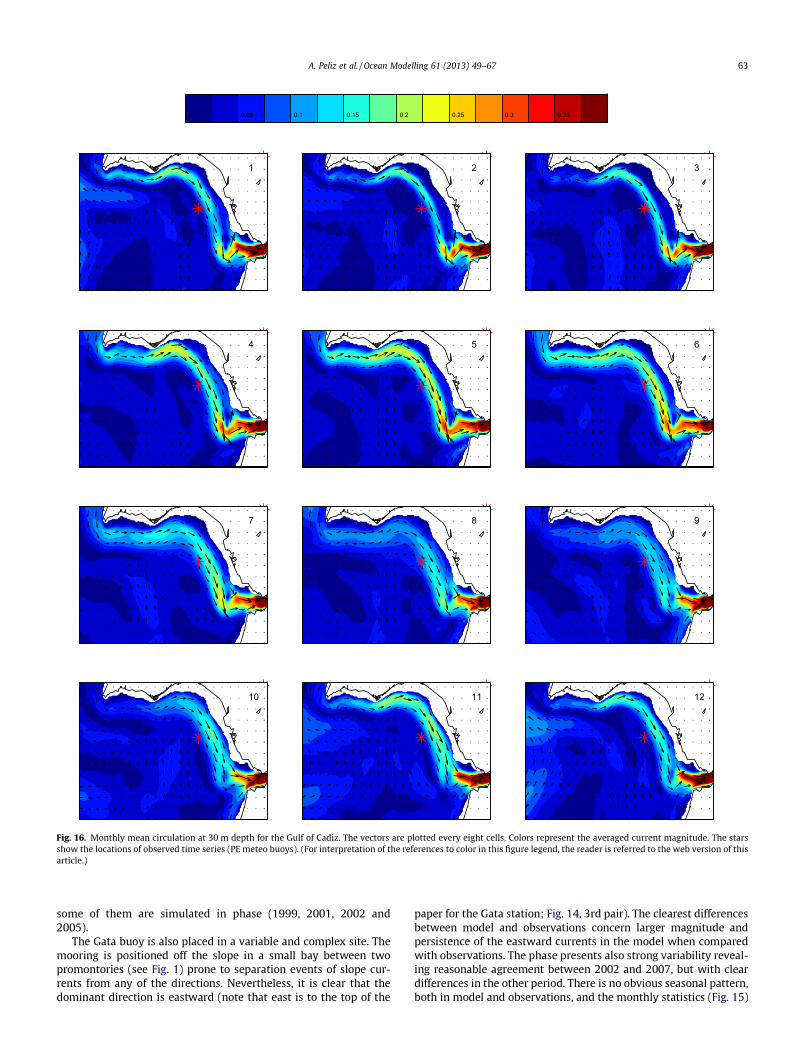
5.1. The slope circulation on the Gulf of Cadiz side

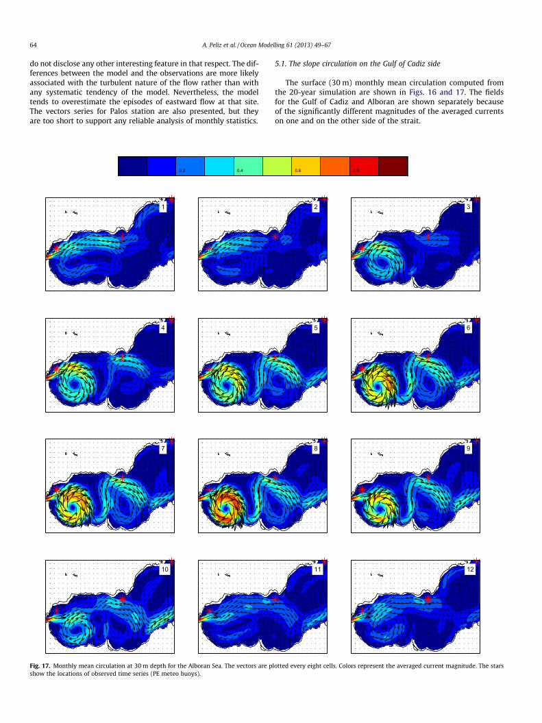
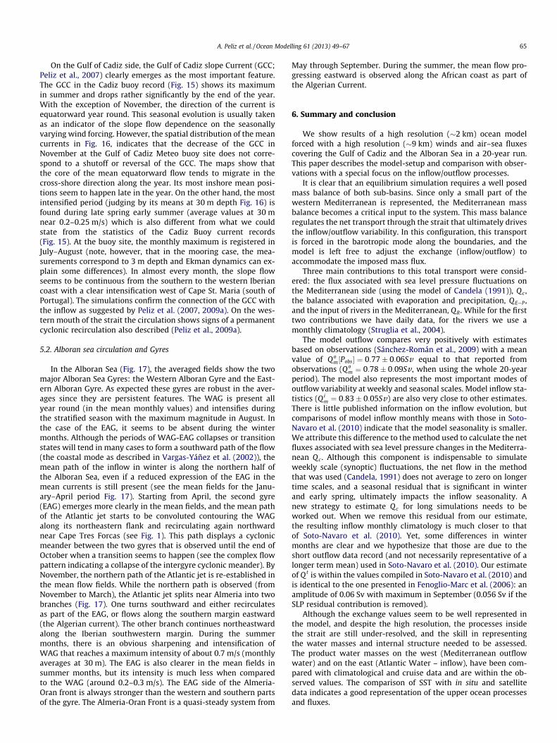
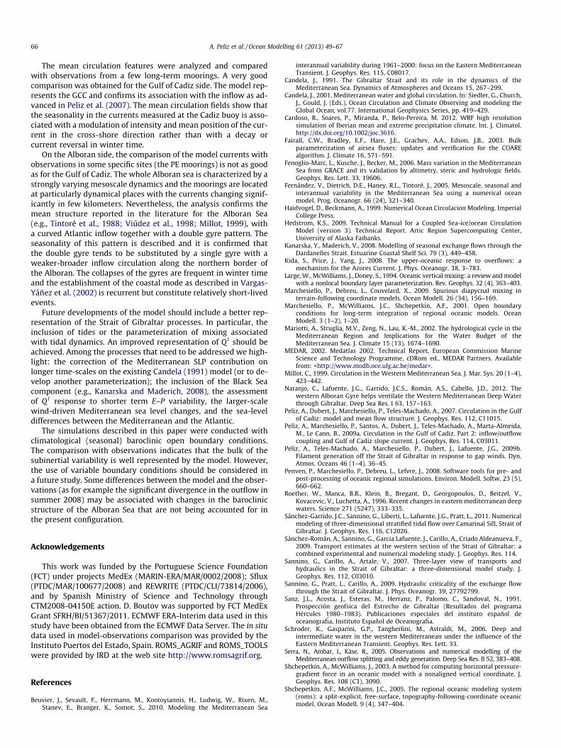
The surface (30 m) monthly mean circulation computed fromthe 20-year simulation are shown in Figs. 16 and 17. The fieldsfor the Gulf of Cadiz and Alboran are shown separately becauseof the significantly different magnitudes of the averaged currentson one and on the other side of the strait.

2 3

5 6

8 9

11 12

8.06.0

otted every eight cells. Colors represent the averaged current magnitude. The stars

A. Peliz et al. / Ocean Modelling 61 (2013) 49–67 65

On the Gulf of Cadiz side, the Gulf of Cadiz slope Current (GCC;Peliz et al., 2007) clearly emerges as the most important feature.The GCC in the Cadiz buoy record (Fig. 15) shows its maximumin summer and drops rather significantly by the end of the year.With the exception of November, the direction of the current isequatorward year round. This seasonal evolution is usually takenas an indicator of the slope flow dependence on the seasonallyvarying wind forcing. However, the spatial distribution of the meancurrents in Fig. 16, indicates that the decrease of the GCC inNovember at the Gulf of Cadiz Meteo buoy site does not corre-spond to a shutoff or reversal of the GCC. The maps show thatthe core of the mean equatorward flow tends to migrate in thecross-shore direction along the year. Its most inshore mean posi-tions seem to happen late in the year. On the other hand, the mostintensified period (judging by its means at 30 m depth Fig. 16) isfound during late spring early summer (average values at 30 mnear 0.2–0.25 m/s) which is also different from what we couldstate from the statistics of the Cadiz Buoy current records(Fig. 15). At the buoy site, the monthly maximum is registered inJuly–August (note, however, that in the mooring case, the mea-surements correspond to 3 m depth and Ekman dynamics can ex-plain some differences). In almost every month, the slope flowseems to be continuous from the southern to the western Iberiancoast with a clear intensification west of Cape St. Maria (south ofPortugal). The simulations confirm the connection of the GCC withthe inflow as suggested by Peliz et al. (2007, 2009a). On the wes-tern mouth of the strait the circulation shows signs of a permanentcyclonic recirculation also described (Peliz et al., 2009a).

5.2. Alboran sea circulation and Gyres

In the Alboran Sea (Fig. 17), the averaged fields show the twomajor Alboran Sea Gyres: the Western Alboran Gyre and the East-ern Alboran Gyre. As expected these gyres are robust in the aver-ages since they are persistent features. The WAG is present allyear round (in the mean monthly values) and intensifies duringthe stratified season with the maximum magnitude in August. Inthe case of the EAG, it seems to be absent during the wintermonths. Although the periods of WAG-EAG collapses or transitionstates will tend in many cases to form a southward path of the flow(the coastal mode as described in Vargas-Yáñez et al. (2002)), themean path of the inflow in winter is along the northern half ofthe Alboran Sea, even if a reduced expression of the EAG in themean currents is still present (see the mean fields for the Janu-ary–April period Fig. 17). Starting from April, the second gyre(EAG) emerges more clearly in the mean fields, and the mean pathof the Atlantic jet starts to be convoluted contouring the WAGalong its northeastern flank and recirculating again northwardnear Cape Tres Forcas (see Fig. 1). This path displays a cyclonicmeander between the two gyres that is observed until the end ofOctober when a transition seems to happen (see the complex flowpattern indicating a collapse of the intergyre cyclonic meander). ByNovember, the northern path of the Atlantic jet is re-established inthe mean flow fields. While the northern path is observed (fromNovember to March), the Atlantic jet splits near Almeria into twobranches (Fig. 17). One turns southward and either recirculatesas part of the EAG, or flows along the southern margin eastward(the Algerian current). The other branch continues northeastwardalong the Iberian southwestern margin. During the summermonths, there is an obvious sharpening and intensification ofWAG that reaches a maximum intensity of about 0.7 m/s (monthlyaverages at 30 m). The EAG is also clearer in the mean fields insummer months, but its intensity is much less when comparedto the WAG (around 0.2–0.3 m/s). The EAG side of the Almeria-Oran front is always stronger than the western and southern partsof the gyre. The Almeria-Oran Front is a quasi-steady system from

May through September. During the summer, the mean flow pro-gressing eastward is observed along the African coast as part ofthe Algerian Current.

6. Summary and conclusion

We show results of a high resolution (�2 km) ocean modelforced with a high resolution (�9 km) winds and air–sea fluxescovering the Gulf of Cadiz and the Alboran Sea in a 20-year run.This paper describes the model-setup and comparison with obser-vations with a special focus on the inflow/outflow processes.

It is clear that an equilibrium simulation requires a well posedmass balance of both sub-basins. Since only a small part of thewestern Mediterranean is represented, the Mediterranean massbalance becomes a critical input to the system. This mass balanceregulates the net transport through the strait that ultimately drivesthe inflow/outflow variability. In this configuration, this transportis forced in the barotropic mode along the boundaries, and themodel is left free to adjust the exchange (inflow/outflow) toaccommodate the imposed mass flux.

Three main contributions to this total transport were consid-ered: the flux associated with sea level pressure fluctuations onthe Mediterranean side (using the model of Candela (1991)), Qc ,the balance associated with evaporation and precipitation, Q E—P ,and the input of rivers in the Mediterranean, QR. While for the firsttwo contributions we have daily data, for the rivers we use amonthly climatology (Struglia et al., 2004).

The model outflow compares very positively with estimatesbased on observations (Sánchez-Román et al., 2009) with a meanvalue of Q o

m½Pobs� ¼ 0:77� 0:06Sv equal to that reported fromobservations (Q o

m ¼ 0:78� 0:09Sv , when using the whole 20-yearperiod). The model also represents the most important modes ofoutflow variability at weekly and seasonal scales. Model inflow sta-tistics (Q i

m ¼ 0:83� 0:05Sv) are also very close to other estimates.There is little published information on the inflow evolution, butcomparisons of model inflow monthly means with those in Soto-Navaro et al. (2010) indicate that the model seasonality is smaller.We attribute this difference to the method used to calculate the netfluxes associated with sea level pressure changes in the Mediterra-nean Q c . Although this component is indispensable to simulateweekly scale (synoptic) fluctuations, the net flow in the methodthat was used (Candela, 1991) does not average to zero on longertime scales, and a seasonal residual that is significant in winterand early spring, ultimately impacts the inflow seasonality. Anew strategy to estimate Qc for long simulations needs to beworked out. When we remove this residual from our estimate,the resulting inflow monthly climatology is much closer to thatof Soto-Navaro et al. (2010). Yet, some differences in wintermonths are clear and we hypothesize that those are due to theshort outflow data record (and not necessarily representative of alonger term mean) used in Soto-Navaro et al. (2010). Our estimateof Q t is within the values compiled in Soto-Navaro et al. (2010) andis identical to the one presented in Fenoglio-Marc et al. (2006): anamplitude of 0.06 Sv with maximum in September (0.056 Sv if theSLP residual contribution is removed).

Although the exchange values seem to be well represented inthe model, and despite the high resolution, the processes insidethe strait are still under-resolved, and the skill in representingthe water masses and internal structure needed to be assessed.The product water masses on the west (Mediterranean outflowwater) and on the east (Atlantic Water – inflow), have been com-pared with climatological and cruise data and are within the ob-served values. The comparison of SST with in situ and satellitedata indicates a good representation of the upper ocean processesand fluxes.

66 A. Peliz et al. / Ocean Modelling 61 (2013) 49–67

The mean circulation features were analyzed and comparedwith observations from a few long-term moorings. A very goodcomparison was obtained for the Gulf of Cadiz side. The model rep-resents the GCC and confirms its association with the inflow as ad-vanced in Peliz et al. (2007). The mean circulation fields show thatthe seasonality in the currents measured at the Cadiz buoy is asso-ciated with a modulation of intensity and mean position of the cur-rent in the cross-shore direction rather than with a decay orcurrent reversal in winter time.

On the Alboran side, the comparison of the model currents withobservations in some specific sites (the PE moorings) is not as goodas for the Gulf of Cadiz. The whole Alboran sea is characterized by astrongly varying mesoscale dynamics and the moorings are locatedat particularly dynamical places with the currents changing signif-icantly in few kilometers. Nevertheless, the analysis confirms themean structure reported in the literature for the Alboran Sea(e.g., Tintoré et al., 1988; Viúdez et al., 1998; Millot, 1999), witha curved Atlantic inflow together with a double gyre pattern. Theseasonality of this pattern is described and it is confirmed thatthe double gyre tends to be substituted by a single gyre with aweaker-broader inflow circulation along the northern border ofthe Alboran. The collapses of the gyres are frequent in winter timeand the establishment of the coastal mode as described in Vargas-Yáñez et al. (2002) is recurrent but constitute relatively short-livedevents.

Future developments of the model should include a better rep-resentation of the Strait of Gibraltar processes. In particular, theinclusion of tides or the parameterization of mixing associatedwith tidal dynamics. An improved representation of Qt should beachieved. Among the processes that need to be addressed we high-light: the correction of the Mediterranean SLP contribution onlonger time-scales on the existing Candela (1991) model (or to de-velop another parameterization); the inclusion of the Black Seacomponent (e.g., Kanarska and Maderich, 2008), the assessmentof Qt response to shorter term E–P variability, the larger-scalewind-driven Mediterranean sea level changes, and the sea-leveldifferences between the Mediterranean and the Atlantic.

The simulations described in this paper were conducted withclimatological (seasonal) baroclinic open boundary conditions.The comparison with observations indicates that the bulk of thesubinertial variability is well represented by the model. However,the use of variable boundary conditions should be considered ina future study. Some differences between the model and the obser-vations (as for example the significant divergence in the outflow insummer 2008) may be associated with changes in the baroclinicstructure of the Alboran Sea that are not being accounted for inthe present configuration.

Acknowledgements

This work was funded by the Portuguese Science Foundation(FCT) under projects MedEx (MARIN-ERA/MAR/0002/2008); Sflux(PTDC/MAR/100677/2008) and REWRITE (PTDC/CLI/73814/2006),and by Spanish Ministry of Science and Technology throughCTM2008-04150E action. D. Boutov was supported by FCT MedExGrant SFRH/BI/51367/2011. ECMWF ERA-Interim data used in thisstudy have been obtained from the ECMWF Data Server. The in situdata used in model-observations comparison was provided by theInstituto Puertos del Estado, Spain. ROMS_AGRIF and ROMS_TOOLSwere provided by IRD at the web site http://www.romsagrif.org.

References

Beuvier, J., Sevault, F., Herrmann, M., Kontoyiannis, H., Ludwig, W., Rixen, M.,Stanev, E., Branger, K., Somot, S., 2010. Modeling the Mediterranean Sea

interannual variability during 1961–2000: focus on the Eastern MediterraneanTransient. J. Geophys. Res. 115, C08017.

Candela, J., 1991. The Gibraltar Strait and its role in the dynamics of theMediterranean Sea. Dynamics of Atmospheres and Oceans 15, 267–299.

Candela, J., 2001. Mediterranean water and global circulation. In: Siedler, G., Church,J., Gould, J. (Eds.), Ocean Circulation and Climate Observing and modeling theGlobal Ocean, vol.77. International Geophysics Series, pp. 419–429.

Cardoso, R., Soares, P., Miranda, P., Belo-Pereira, M. 2012. WRF high resolutionsimulation of Iberian mean and extreme precipitation climate. Int. J. Climatol.http://dx.doi.org/10.1002/joc.3616.

Fairall, C.W., Bradley, E.F., Hare, J.E., Grachev, A.A., Edson, J.B., 2003. Bulkparameterization of airsea fluxes: updates and verification for the COAREalgorithm. J. Climate 16, 571–591.

Fenoglio-Marc, L., Kusche, J., Becker, M., 2006. Mass variation in the MediterraneanSea from GRACE and its validation by altimetry, steric and hydrologic fields.Geophys. Res. Lett. 33, 19606.

Fernández, V., Dietrich, D.E., Haney, R.L., Tintoré, J., 2005. Mesoscale, seasonal andinterannual variability in the Mediterranean Sea using a numerical oceanmodel. Prog. Oceanogr. 66 (24), 321–340.

Haidvogel, D., Beckmann, A., 1999. Numerical Ocean Circulacion Modeling. ImperialCollege Press.

Hedstrom, K.S., 2009. Technical Manual for a Coupled Sea-ice/ocean CirculationModel (version 3). Technical Report. Artic Region Supercomputing Center,University of Alaska Faibanks.

Kanarska, Y., Maderich, V., 2008. Modelling of seasonal exchange flows through theDardanelles Strait. Estuarine Coastal Shelf Sci. 79 (3), 449–458.

Kida, S., Price, J., Yang, J., 2008. The upper-oceanic response to overflows: amechanism for the Azores Current. J. Phys. Oceanogr. 38, 3–783.

Large, W., McWilliams, J., Doney, S., 1994. Oceanic vertical mixing: a review and modelwith a nonlocal boundary layer parameterization. Rev. Geophys. 32 (4), 363–403.

Marchesiello, P., Debreu, L., Couvelard, X., 2009. Spurious diapycnal mixing interrain-following coordinate models. Ocean Modell. 26 (34), 156–169.

Marchesiello, P., McWilliams, J.C., Shchepetkin, A.F., 2001. Open boundaryconditions for long-term integration of regional oceanic models. OceanModell. 3 (1–2), 1–20.

Mariotti, A., Struglia, M.V., Zeng, N., Lau, K.-M., 2002. The hydrological cycle in theMediterranean Region and Implications for the Water Budget of theMediterranean Sea. J. Climate 15 (13), 1674–1690.

MEDAR, 2002. Medatlas 2002. Technical Report, European Commission MarineScience and Technology Programme, cDRom ed., MEDAR Partners. Availablefrom: <http://www.modb.oce.ulg.ac.be/medar>.

Millot, C., 1999. Circulation in the Western Mediterranean Sea. J. Mar. Sys. 20 (1–4),423–442.

Naranjo, C., Lafuente, J.G., Garrido, J.C.S., Román, A.S., Cabello, J.D., 2012. Thewestern Alboran Gyre helps ventilate the Western Mediterranean Deep Waterthrough Gibraltar. Deep Sea Res. I 63, 157–163.

Peliz, A., Dubert, J., Marchesiello, P., Teles-Machado, A., 2007. Circulation in the Gulfof Cadiz: model and mean flow structure. J. Geophys. Res. 112, C11015.

Peliz, A., Marchesiello, P., Santos, A., Dubert, J., Teles-Machado, A., Marta-Almeida,M., Le Cann, B., 2009a. Circulation in the Gulf of Cadiz. Part 2: inflow/outflowcoupling and Gulf of Cadiz slope current. J. Geophys. Res. 114, C03011.

Peliz, A., Teles-Machado, A., Marchesiello, P., Dubert, J., Lafuente, J.G., 2009b.Filament generation off the Strait of Gibraltar in response to gap winds. Dyn.Atmos. Oceans 46 (1–4), 36–45.

Penven, P., Marchesiello, P., Debreu, L., Lefvre, J., 2008. Software tools for pre- andpost-processing of oceanic regional simulations. Environ. Modell. Softw. 23 (5),660–662.

Roether, W., Manca, B.B., Klein, B., Bregant, D., Georgopoulos, D., Beitzel, V.,Kovacevic, V., Luchetta, A., 1996. Recent changes in eastern mediterranean deepwaters. Science 271 (5247), 333–335.

Sánchez-Garrido, J.C., Sannino, G., Liberti, L., Lafuente, J.G., Pratt, L., 2011. Numericalmodeling of three-dimensional stratified tidal flow over Camarinal Sill, Strait ofGibraltar. J. Geophys. Res. 116, C12026.

Sánchez-Román, A., Sannino, G., Garcia Lafuente, J., Carillo, A., Criado Aldeanueva, F.,2009. Transport estimates at the western section of the Strait of Gibraltar: acombined experimental and numerical modeling study. J. Geophys. Res. 114.

Sannino, G., Carillo, A., Artale, V., 2007. Three-layer view of transports andhydraulics in the Strait of Gibraltar: a three-dimensional model study. J.Geophys. Res. 112, C03010.

Sannino, G., Pratt, L., Carillo, A., 2009. Hydraulic criticality of the exchange flowthrough the Strait of Gibraltar. J. Phys. Oceanogr. 39, 27792799.

Sanz, J.L., Acosta, J., Esteras, M., Herranz, P., Palomo, C., Sandoval, N., 1991.Prospección geofsica del Estrecho de Gibraltar (Resultados del programaHércules 1980–1983). Publicaciones especiales del instituto español deoceanografı́a, Instituto Español de Oceanografı́a.

Schroder, K., Gasparini, G.P., Tangherlini, M., Astraldi, M., 2006. Deep andintermediate water in the western Mediterranean under the influence of theEastern Mediterranean Transient. Geophys. Res. Lett. 33.

Serra, N., Ambar, I., Käse, R., 2005. Observations and numerical modelling of theMediterranean outflow splitting and eddy generation. Deep Sea Res. II 52, 383–408.

Shchepetkin, A., McWilliams, J., 2003. A method for computing horizontal pressure-gradient force in an oceanic model with a nonaligned vertical coordinate. J.Geophys. Res. 108 (C3), 3090.

Shchepetkin, A.F., McWilliams, J.C., 2005. The regional oceanic modeling system(roms): a split-explicit, free-surface, topography-following-coordinate oceanicmodel. Ocean Modell. 9 (4), 347–404.

A. Peliz et al. / Ocean Modelling 61 (2013) 49–67 67

Skamarock, W., 2008. A Description of the Advanced Research WRF Version 3.Technical Report, NCAR, Technical Note TN-475-STR, 113 pp.

Smith, W., Sandwell, D., 1997. Global sea floor topography from satellite altimetryand ship depth soundings. Science 277 (5334), 1956–1962.

Soares, P., Cardoso, R., de Medeiros, J., Miranda, P., Belo-Pereira, M., Espirito-Santo, F.,2012. WRF high resolution dynamical downscaling of ERA-Interim for Portugal.Climate Dyn. 39, 2497–2522, http://dx.doi.org/10.1007/s00382-012-1315-2.

Soto-Navaro, J., Criado-Aldeanueva, F., Garcia-Lafuent, J.S.-R.A., 2010. Estimation ofthe atlantic inflow through the Strait of Gibraltar from climatological and in situdata. J. Geophys. Res. 115, C10023.

Struglia, M.V., Mariotti, A., Filograsso, A., 2004. River discharge into theMediterranean Sea: climatology and aspects of the observed variability. J.Climate 17 (24), 4740–4751.

Tintoré, J., La Violette, P.E., Blade, I., Cruzado, A., 1988. A study of an intense densityfront in the eastern Alboran sea: the Almeria-Oran front. J. Phys. Oceanogr. 18,1384–1397.

Vargas-Yáñez, M., Plaza, F., Garcı́a-Lafuente, J., Sarhan, T., Vargas, J., Vélez-Belchi, P.,2002. About the seasonal variability of the Alboran sea circulation. J. Mar. Sys.35 (3–4), 229–248.

Viúdez, A., Pinot, J.-M., Haney, R.L., 1998. On the upper layer circulation in theAlboran sea. J. Geophys. Res. 103 (C10), 21653–21666.

Xu, X., Chassignet, E., Price, J., Ozgokmen, T., Peters, H., 2007. A regionalmodeling study of the entraining Mediterranean outflow. J. Geophys. Res.112, C12005.

Zervakis, V., Georgopoulos, D., Karageorgis, A.P., Theocharis, A., 2004. On theresponse of the aegean sea to climatic variability: a review. Int. J. Climatol. 24(14), 1845–1858.

Zunino, P., Schroeder, K., Nez, M.V.-Y., Gasparini, G., Coppola, L., García-Martínez,M., Moya-Ruiz, F., 2012. Effects of the Western Mediterranean Transition on theresident water masses: pure warming, pure freshening and pure heaving. J. Mar.Sys. 9697 (0), 15–23.