THE GRAND TOUR:

KEYNES AND GOODWIN GO TO GREECE

Eduardo A. Haddad

Natalia Cotarelli

Thiago C. Simonato

Vinicius A. Vale

Jaqueline C. Visentin

TD Nereus 05-2017

São Paulo

2017

1

The Grand Tour: Keynes and Goodwin go to Greece

Eduardo A. Haddad, Natalia Cotarelli, Thiago C. Simonato, Vinicius A. Vale and

Jaqueline C. Visentin

Abstract. The impact of the crisis in the Greek economy was not uniform among the

regions, threatening socioeconomic cohesion. In this paper, we explore the concept of

the income multiplier in a multi-regional setting, in the context of the Greek recession,

showing empirical evidence for the increasing magnitude of the multiplier during the

recession period. The main results reveal a complex system of interregional relations on

some of whose structural characteristics the cyclical reaction paths of the regions

depend. In this case, the use of fiscal instruments to stimulate local activity in the

regions may bring about important implications for regional inequality in Greece.

1. Introduction

Robert Solow (Solow, 2015) has recently commented on Richard Goodwin’s article

‘The Multiplier as a Matrix’ (Goodwin, 1949) recalling the analogy between the

Leontief-like matrix multiplier and the Kahn-Keynes multiplier.1 By including

households as one of the sectors, Goodwin’s multi-sectorial approach has paved the way

to replicate Kahn-Keynes by calculating an aggregate national income multiplier as a

weighted average of all sector multipliers.

Having Wassily Leontief as its most influential source of inspiration, the quest for

relaxing the aggregative nature of the Keynesian system has nudged not only

Goodwin’s initial scientific accomplishments but also other early authors’, especially

Chipman (1950), who developed, at the same time as Goodwin, the notion of sector

multipliers. The idea that a net increase in the rate of home investment (and other

autonomous injections) propagates in the entire system generating higher-order effects

is even more appealing in a multi-sectorial context. Rather than attempting to create a

complete model of the economy, the main interest was to trace some of the effects of

such injections in the system (Solow, 2015).

While, for the sake of simplicity, Goodwin has focused on a closed economy in his

1949 article, using direct references to Keynes, Chipman acknowledged in his more

1 Kahn (1931) and Keynes (1936).

2

general setting the strong influence from the work by Fritz Machlup on the foreign-trade

multiplier. Machlup (1943) had presented a framework that considered ripple effects in

the context of international trade. He has initially developed the idea of the foreign trade

multiplier in a demand-driven two-country framework, in which an increase in

autonomous income in country A generates, through import leakages, an increase in the

income of country B, i.e. part of the increase in the income of A would be spent on

imports from country B. Part of this income transfer from A to B, in a second round,

would return to A via A’s exports to B. This process would continue until the income

transfers became negligible. Building on that, Metzler (1950) attempted to generalize

this idea by considering a model of an economic system composed of n regions or

countries. Goodwin (1980) revisited this debate presenting a simple, largely static,

prototypical analysis using statistically derived data to illustrate how the foreign trade

matrix multiplier could be decomposed so as to separate out the internal effects of a

demand expansion (or contraction) from the international feedback operating through

the trade network.

Walter Isard further developed Machlup-Chipmann’s foreign trade multiplier in the

context of regions within a single country. As this notion worked for countries linked by

trade flows, this could be applied for domestic trading regions as well. In a simplified

formulation, the interregional trade multiplier would indicate the multiple regional

income as the sum of regional investments and exports. Thus, changes in regional

income would result from (and as a multiple of) a change in regional investment,

exports, or both. The key point is that, in complex economic structures, neither sectors

nor regions are isolated entities. By employing a multi-sectorial interregional

framework, one may learn something about the cyclical sensitivities of other regions

and the ways in which their cycles may be spread to her own region. This type of study

leads to a more precise formulation of multiplier effects and of the mechanisms by

which cycles are spatially transmitted within the system of regions. It centres around the

interregional trade multiplier, a concept closely akin to Keynesian doctrine (Isard,

1960).

In all those instances, the theory embedded in the concept of multipliers is short-run in

nature in the same sense as Keynes’ General Theory is a short-run theory: it is a static

theory of income and not a theory of growth, which makes it less applicable to longer

3

periods of analysis (Metzler, 1950). The magnitude of this well-known macroeconomic

mechanism has been object of controversy regarding its application in the realm of

economic policies. Charles (2016) reports on several recent studies that have shown that

the fiscal multiplier is endogenous to the level of economic activity, increasing during

recessions and decreasing during the boom. In fact, Auerbach and Gorodnichenko

(2012) show that, in a recession, the multiplier may be larger, especially at short

horizons. Despite contested by mainstream economists, the logical policy implication

recommends the expansion of public expenditures during a recession period to sustain

effective demand and the level of profits to increase employment.

The aforementioned theoretical developments, associated with seminal works by

Keynes and Goodwin, provided the bases for a strand of empirical research dedicated to

understand economic systems, structures and processes, and their change through time

and space. A body of literature has emerged relying on historical input-output databases

as valuable sources of information for uncovering some of the important dimensions of

structural change in an economy, and for unravelling the various sources of growth of

national and regional economies (e.g. Feldman et al., 1987; Dewhurst, 1993; Sonis et

al., 1996; Dietzenbacher and Los, 2000; Hitomi et al., 2000; Romero et al., 2009; Zhang

and Lahr, 2014). The common focus relies very often on the role played by technical

change and changes in final demand, the latter reflecting changes in social preferences

(Haddad et al., 2014). Other approaches based on input-output systems have attempted

to analyse the structure of multi-regional trade flows. Feedback loop analysis has been

used for both interregional (Sonis et al., 1995; Sonis et al., 2001) and intercountry input-

output tables (Sonis et al., 1993) providing an opportunity to examine the hierarchy of

intra- and interregional trade flows within an integrated economic system.

Such framework is particularly interesting for assessing the spatial propagation of the

Greek crisis. From 2010 to 2013, period of our analysis, real GDP fell almost 23% in

Greece, with a decrease in government expenditures by 25% and in investments by

roughly 45%, with a small increase in international exports by less than 2%. In the same

period, real GRP from the 13 NUTS-2 regions varied from -14.7%, in Western

Macedonia to -31.9% in Eastern Macedonia and Thrace. In the case of Greece,

geography has played an important role since the spatial pattern of the initial impacts of

the austerity measures was influenced by the geographical presence of the public sector.

4

However, when taking into account indirect and induced effects, the regional structure

of the Greek economy has also influenced the spatial propagation of the impacts

through a complex diffusion of the multiplier effects. Though small, the Greek economy

is not internally homogenous, presenting variations across both industries and regions.

Thus, the anti-crisis, austerity, measures taken in Greece, though horizontal in their

nature, may have significantly differentiated implications across space (Psycharis et al.,

2014).

In what follows, we present some basic information on the uneven regional impacts of

the Greek crisis to motivate further our case study. We will use a unique database

comprised of two fully specified interregional input-output tables for Greece, estimated

for the years 2010 and 2013. Despite some difficulties associated with the process of

estimation of the database that generate some caveats in the forthcoming analysis,

discussed in the coming sessions, we provide some insights to be further explored in

future studies. What has happened to the national income multiplier during this period?

Have Greek regions adjusted in different ways with implications for the changing value

of their respective multipliers, and, consequently, for the design of countercyclical

regional policy prescriptions?

Using techniques of structural decomposition analysis (SDA) for comparing different

economic structures in the context of partitioned input-output systems, we will be able

to assess the main driving forces of the changes faced by the Greek regions in the first

years of the economic recession and fiscal austerity. We show that changes in final

demand – mainly in investment and government demand – were the main drivers of the

setback of the economy. However, technical change was also an important element to

drive changes in regional income. In spite of its smaller magnitude, it has played

different roles for different regions. While in some regions technical coefficients have

adjusted through stronger internal linkages that favoured the internalization of the

multiplier effects, other regions increased their dependence upon the rest of the system,

increasing the existing leakages. Overall, the national income multiplier for Greece

increased by 5.9% from 2010 to 2013. Moreover, all regions also faced increases in

their value added (income) multipliers during the recession period, notwithstanding

differences in the intensity and in the spatial distribution of the changes.

5

Thus, the objectives of this paper are twofold. On one hand, we bring additional

evidence for the internal propagation of the Greek crisis from a regional perspective. On

the other hand, we look at the interdependence of technology, domestic and

international trade linkages, and components of aggregate demand as possible sources

of the variation in the spread of the effects initiated with the austerity program. While

the results are to be qualified, we hope they will serve to shed light on the mechanisms

of changes in regional income in the context of the Greek crisis and to stimulate further

work in this line of research.

2. Regional Dimensions of the Greek Crisis

The effects of the economic crisis in Greece have been the object of different studies.

One of the important elements of the Greek crisis refers to the alleged fact that the

Greek authorities had falsified debt information. Both the deficit and the accumulated

stock of debt were far higher than the official numbers. After the news that Greece

distorted its statistics during a number of years, Greek securities were downgraded to

junk bonds status and the prices of Greek bonds tumbled with the risk of insolvency of

the country. In this context, fiscal austerity was imposed upon the Greek governments in

exchange for Europe Union bailout assistance.

Most of the studies that have analysed the Greek crisis have as their main focus the

impact of the austerity measures on the country’s economy. The modelling-based

argument that measures of fiscal austerity in Greece have failed, raised by Betz and

Carayannis (2015), suggests that the Polak Model (Polak, 1957), that was used to justify

the policy of austerity in assisting an economically troubled nation, did not immediately

solve the fiscal problem but only deepened the Greek fiscal crisis, increasing

unemployment, recession and government instability. In his diagnostics on the

contemporary austerity policies, of which the Greek case was part, Boyer (2012)

identifies as one of the fallacies in the debate the neglect of crowding in and competitive

mechanisms that could quickly stop the downwards adjustments and trigger a vigorous

recovery of the economies under stress.

Along with Betz and Carayannis (2015), Krugman (2013) defended that the Greek crisis

was a “godsend” for anti-Keynesians that had been warning how dangerous fiscal

6

profligacy can be. At that time, many economists suggested that a certain level of debt

hurts growth2, and a theory known as “expansionary austerity”, which defends that cuts

in the government spending increase the output, became remarkably influential.

However, data for the Greek economy have shown that these propositions were not

necessarily right. As stated by Paul Krugman, the data proved that the austerity program

has had major adverse economic effects. More than that, the downturns in the economy

were more or less proportional to the degree of austerity.

The deterioration in the Greek situation after the adoption of fiscal austerity measures

was such that, in 2015, prominent economists, including Thomas Piketty, Jeffrey Sachs

and Dani Rodrik, wrote an open letter to ask Chancellor Angela Merkel to rethink the

punitive and failed program on the recent years that “crushed the Greek economy, led to

mass unemployment and a collapse of banking system”. According to these economists,

the humanitarian impact was colossal. In fact, fiscal consolidation through spending

cuts and tax increases has been shown to have raised the risk of increased poverty and

inequality (Matsaganis and Leventi, 2013).

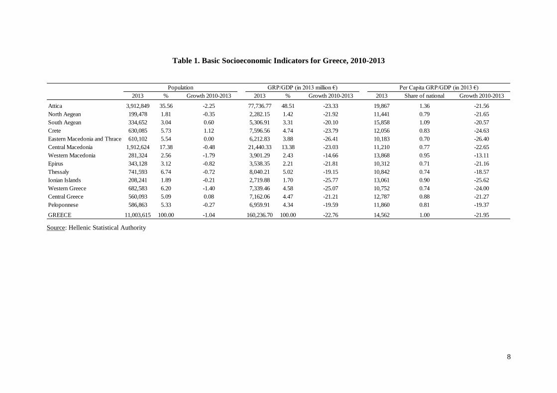
Moreover, the impact of the crisis in the Greek economy was not uniform among the

regions, threatening socioeconomic cohesion (see Table 1 and Figure 1). Its

‘geographical footprint’ has been examined, for instance, in Psycharis et al. (2014) who

have shown that metropolitan areas and regions that are based on manufacturing

activities seem to have been more vulnerable to the crisis while places that are based on

tourism, such as islands, were usually more resistant. This result is confirmed in

Artelaris (2017) that presented further evidence that less advanced and/or urbanised

regions are more resilient during the period of crisis. Sectorial composition is also used

as an element to explain regional differences in unemployment effects (Karafolas and

Alexandrakis, 2015).

Spatial concentration of economic activities and the degree of regional specialization or

diversification seem to affect regional reactions to economic shocks (Richardson, 1969;

Attaran, 1986; Berry, 1988; Martin, 2012; Eraydin, 2016; Martin et al., 2016).

Empirical evidence for Greece suggests that tourism has been among the most resilient

2 Reinhart and Rogoff (2010), for instance, argued that not just debt hurts growth, but that there is a

threshold when debt is higher than 90% of GDP, economic growth stalls.

7

sectors of the Greek economy and therefore regions that are specialized in tourism-

based activities are also more resilient to the crisis. On the contrary, regions specialized

in sectors such as banks and real estate, financial intermediaries and insurance

companies that are more exposed to international fluctuations and more affected by the

economic crisis tended to be more affected during the recession (Psycharis et al., 2014).

In the case of tourism, nonetheless, Papatheodorou and Arvanitis (2014) claim that any

generalization should be treated with caution due to the complex character of the

particular activity and the inherent asymmetries between domestic and international

tourism. They suggest that, in the context of the crisis, a new geography of tourism

seems to have emerged in Greece where the clear losers are those regions that had

specialized predominantly in domestic tourism.

Figure 1. Change in Regional Unemployment Rate: Greece, 2010-2013

Source: EUROSTAT

8

Table 1. Basic Socioeconomic Indicators for Greece, 2010-2013

Source: Hellenic Statistical Authority

2013 % Growth 2010-2013 2013 % Growth 2010-2013 2013 Share of national Growth 2010-2013

Attica 3,912,849 35.56 -2.25 77,736.77 48.51 -23.33 19,867 1.36 -21.56

North Aegean 199,478 1.81 -0.35 2,282.15 1.42 -21.92 11,441 0.79 -21.65

South Aegean 334,652 3.04 0.60 5,306.91 3.31 -20.10 15,858 1.09 -20.57

Crete 630,085 5.73 1.12 7,596.56 4.74 -23.79 12,056 0.83 -24.63

Eastern Macedonia and Thrace 610,102 5.54 0.00 6,212.83 3.88 -26.41 10,183 0.70 -26.40

Central Macedonia 1,912,624 17.38 -0.48 21,440.33 13.38 -23.03 11,210 0.77 -22.65

Western Macedonia 281,324 2.56 -1.79 3,901.29 2.43 -14.66 13,868 0.95 -13.11

Epirus 343,128 3.12 -0.82 3,538.35 2.21 -21.81 10,312 0.71 -21.16

Thessaly 741,593 6.74 -0.72 8,040.21 5.02 -19.15 10,842 0.74 -18.57

Ionian Islands 208,241 1.89 -0.21 2,719.88 1.70 -25.77 13,061 0.90 -25.62

Western Greece 682,583 6.20 -1.40 7,339.46 4.58 -25.07 10,752 0.74 -24.00

Central Greece 560,093 5.09 0.08 7,162.06 4.47 -21.21 12,787 0.88 -21.27

Peloponnese 586,863 5.33 -0.27 6,959.91 4.34 -19.59 11,860 0.81 -19.37

GREECE 11,003,615 100.00 -1.04 160,236.70 100.00 -22.76 14,562 1.00 -21.95

Population GRP/GDP (in 2013 million €) Per Capita GRP/GDP (in 2013 €)

9

3. Empirical Strategy and Data Treatment

We use SDA to identify the drivers of Greece’s recession at the regional level between

2010 and 2013, from both the production side and the final demand side. From the

production side, we analyse the impacts of changes in value added generation and the

production structure, taking into full consideration the systemic role of imported inputs,

and inter-regional trade of intermediate goods. In the final demand side, we analyse the

impacts of changes not only in the level but also in the composition of final demand,

especially capital investment, government expenditures and export demand of each

region. We make use of a set of interregional input-output tables for Greece in the

empirical analysis.3

3.1. Structural Decomposition Analysis (SDA)

Structural decomposition analysis (SDA) aims at decomposing the total amount of

change in some aspect of an economy. In an input-output framework, the total change in

gross output – or in any economic variable that is function of it – can be broken into

technical changes, final-demand changes, and other elements of the system. In the case

of multi-regional systems, the Leontief-like multiplier matrix contains information on

both technical coefficients and trade proportions (Miller and Blair, 2009).

Considering that we have the input-output tables for two years, 2010 and 2013, we

endogeneise the household sector so that we are able to incorporate links between factor

payments and household expenditures. Moreover, we transform the Leontief matrix to

make adequate comparisons in terms of income (value added) multipliers. The use of

value added instead of gross output, not only is more adequate to couple the discussion

to the Keynesian multiplier literature, but also it helps to unravel more accurately the

role played by the service sectors in the Greek economy, usually with higher contents of

value added per unit of output, and with an important role in the economic structure of

the country.4

The closed input–output model, with r regions, n sectors and households endogenous,

can be represented by

3 The database is available as a supplementary file.

4 The share of the tertiary sector in Greek GDP was 85.5% in 2010, and 82.8% in 2013.

10

(1)

and

(2)

where denotes the [r x (n + 1)]-element column vector of gross outputs in year t;

the [r x (n + 1)]-element vector of final demands in year t; the [r x (n + 1)] x [r x (n +

1)] input–output (or technical, or direct input) coefficients matrix with households

included in year t; is the identity matrix; and is the Leontief inverse or multipliers

matrix in year t for the closed (household endogenous).5

From (2) and a set of value added input coefficients – calculated as value added

(income) per euro of output in sector n in region r at time t ( ), we can represent value

added ( ) as function of in year t as

(3)

Where is a matrix with ratios of value added to gross output (value added input

coefficients) on the diagonal and zeros elsewhere (off-diagonal).

Then the observed change in value added over the period (t = 2010, 2013) is

(4)

In order to decompose the total change in value added and remove the influence of price

changes, all data are expressed in prices of 2013. Then one possible decomposition of

changes in value added (3) can be represented as6

5 See Miller and Blair (2009) for more details.

6 This is not the only decomposition possible. See Dietzenbacher and Los (1998) and Miller and Blair

(2009) for a discussion of a wide variety of possible alternatives. We also refer to these authors for

mathematical details, including additive decompositions with products of more than two terms.

11

⁄ ( )

⁄

⁄ ( )

(5)

where the first term on the right-hand side, ( ), is the value-

added-input-coefficient change; the second term, ,

is the direct-coefficient change; and the third term, ( ), the

final-demand change.

3.2. Interregional Input-Output Systems for Greece, 2010 and 2013

The input-output tables used in our calculations reflect the economic structure of the

Greek economy in two points in time (2010 and 1013). They consider the 13 NUTS 2

regions in Greece whose economies are disaggregated in 44 sectors. The tables are in

constant 2013 prices. We have generated the database using the IIOAS (Interregional

Input-Output Adjustment System) method. The IIOAS is a hybrid method that combines

data made available by official agencies, such as the Hellenic Statistical Authority and

EUROSTAT, with non-census techniques for the estimation of unavailable information.

The main advantages of the IIOAS are its consistency with information from the

National Accounts Statistics and the flexibility of its regionalization process, which can

be applied to any country that: (i) publishes standard make and use tables; and (ii)

provides a regional information system at the sectorial level. Such flexibility can be

attested by recent applications for distinct interregional systems: interisland model for

the Azores (Haddad et al., 2015), interregional models for Colombia (Haddad et al.,

2016a), Egypt (Haddad et al., 2016b), Lebanon (Haddad, 2014), Morocco (Haddad et

al., 2017a), and Brazil (Haddad et al., 2017b).7

7 Detailed information on the estimation process is documented in the aforementioned applications.

12

Interregional Linkages

We can compute the contribution to regional income of final demand from different

origins. In an integrated interregional system, regional income depends, among others,

on demand originating in the own region and, depending on the degree of interregional

integration, on demand from outside the region.

Using basic input-output techniques, we consider the interdependence among sectors in

different regions through the analysis of the complete direct coefficients portion of the

interregional input-output table. To illustrate the nature of interregional linkages in

Greece, we provide, in Tables 2 and 3, some summary indicators of the structure of the

Greek economy derived from the Leontief inverse (multipliers) matrix for 2013.

The column multipliers derived from were computed (see Miller and Blair, 2009).

An income or value added multiplier is defined for each sector j, in each region r, as the

total value added in all sectors and in all regions of the economy that is necessary in

order to satisfy a dollar’s worth of final demand for sector j’s output. The multiplier

effect can be decomposed into intra-regional (internal multiplier) and interregional

(external multiplier) effects, the former representing the impacts on the value added of

sectors within the region where the final demand change was generated, and the latter

showing the impacts on the other regions of the system (interregional spillover effects).

Table 2 shows the intra-regional and interregional shares for the weighted average total

value added multipliers in the 13 NUTS 2 regions in Greece as well as the equivalent

shares for the direct, indirect an induced effects of a unit change in final demand in each

sector in each region net of the initial injection, i.e., the total income multiplier effect

net of the initial change. The entries are shown in percentage terms, providing insights

into the degree of dependence of each region on the other regions. Noteworthy are the

results for Attica, the most self-sufficient region, where the average intra-regional flow-

on effects from a unit change in sectorial final demand are the highest: the average net

effect exceeds 80%. For some regions, located in Northern and Central Mainland

Greece, the degree of regional self-sufficiency is much lower, and the intra-regional

flow-on effects, on the average, are much lower than the total interregional effects.

13

A complementary analysis to the multiplier approach is presented in Table 3, in which

we decompose regional income by taking into account not only the multiplier structure,

but also the structure of final demand in the 13 domestic and the foreign regions (Sonis

et al., 1996). We calculate the contributions of the components of final demand from

different areas. The results reveal that, on average, the self-generated component of

income in each region, i.e. the share of value added generated by demand within the

region, is lower in those regions that present higher dependency upon the rest of the

country and the rest of the world. The demand for foreign exports is very relevant for

not only Attica but also for other regions with bigger metropolitan areas such as Central

Macedonia (Thessaloniki) and Central Greece (Patras). Its contribution can reach more

than one-fifth of the regional income (16.3% for the country as a whole), as is the case

of Central Greece (21.9%). There are also some cases of stronger dependency upon the

rest of the country, as it is the case of the dependency of various regions on Attica’s

demand, and, to a lesser degree, the dependency of regions in the North of the country

on Central Macedonia’s demand.

A more systematic approach to visualise the influence of final demand from different

regions is to map the column original estimates that generated Table 3. The results,

illustrated in Figure 2, provide an attempt to reveal the spatial patterns of income

dependence upon specific sources of final demand. The 13 regions are grouped in seven

different categories in each map, so that darker colours represent higher values.

14

Table 2. Regional Percentage Distribution of the Average Total Value Added

Multipliers: Greece, 2013 (in %)

Table 3. Components of the Decomposition of GRP/GDP based on the Sources of

Final Demand: Greece, 2013 (in %)

Intra-regional share Interregional share Intra-regional share Interregional share

R1 Attica 95.2 4.8 80.1 19.9

R2 North Aegean 87.2 12.8 47.6 52.4

R3 South Aegean 90.6 9.4 59.7 40.3

R4 Crete 91.6 8.4 66.6 33.4

R5 Eastern Macedonia and Thrace 83.6 16.4 38.4 61.6

R6 Central Macedonia 86.4 13.6 48.5 51.5

R7 Western Macedonia 81.1 18.9 28.0 72.0

R8 Epirus 81.9 18.1 35.3 64.7

R9 Thessaly 82.7 17.3 33.6 66.4

R10 Ionian Islands 86.8 13.2 50.1 49.9

R11 Western Greece 85.6 14.4 43.6 56.4

R12 Central Greece 78.8 21.2 30.9 69.1

R13 Peloponnese 82.7 17.3 36.4 63.6

Value Added Multiplier Net Value Added Multiplier

R1 R2 R3 R4 R5 R6 R7 R8 R9 R10 R11 R12 R13 ROW

Attica R1 58.5 0.6 0.3 0.7 2.1 6.6 1.4 1.3 3.1 0.3 2.5 2.5 2.8 17.4

North Aegean R2 9.0 68.4 0.2 0.3 1.6 4.7 0.9 0.6 1.3 0.1 0.9 0.8 0.7 10.4

South Aegean R3 30.1 0.9 31.0 0.8 3.0 10.6 2.1 1.4 2.9 0.2 2.3 1.8 2.0 11.0

Crete R4 22.7 0.6 0.3 44.5 2.9 5.8 1.2 1.0 2.1 0.2 1.9 1.5 1.7 13.8

Eastern Macedonia and Thrace R5 8.2 0.5 0.2 0.3 65.6 5.4 1.0 0.7 1.4 0.2 0.8 0.9 0.7 14.1

Central Macedonia R6 11.5 0.6 0.2 0.4 2.2 57.4 2.5 1.3 3.4 0.2 1.1 1.5 0.9 16.6

Western Macedonia R7 18.8 0.7 0.3 0.6 2.9 13.1 33.9 2.4 4.1 0.5 2.3 2.1 1.9 16.4

Epirus R8 13.1 0.4 0.1 0.4 1.5 7.4 2.7 55.5 2.2 0.4 1.5 1.5 1.2 12.2

Thessaly R9 14.0 0.4 0.2 0.4 1.5 9.0 1.8 1.1 53.2 0.2 1.1 2.3 1.0 13.9

Ionian Islands R10 23.7 0.5 0.1 0.3 2.2 11.4 3.1 3.2 3.4 34.5 2.6 2.0 1.8 11.2

Western Greece R11 17.0 0.4 0.2 0.4 1.1 3.8 1.0 1.0 1.4 0.2 56.9 1.2 1.6 14.1

Central Greece R12 21.0 0.5 0.2 0.6 1.6 7.1 1.3 1.0 3.8 0.2 1.5 37.7 1.4 21.9

Peloponnese R13 21.2 0.4 0.2 0.5 1.2 3.9 0.8 0.8 1.5 0.2 1.7 1.2 48.8 17.5

GREECE 36.9 1.5 1.2 2.7 4.3 13.6 2.4 2.5 5.4 0.8 4.5 3.6 4.1 16.3

Origin of Final Demand

GR

P/G

DP

15

Figure 2. Identification of Regions Relatively More Affected by a Specific Regional

Demand, by Origin of Final Demand

16

4. Empirical Results and Main Findings

Table 4 presents the results of the SDA for total value added (see also Figure 3). Greek

GDP decreased 22.78% from 2010 to 2013. At the aggregate level, it reveals the

qualitative results with GDP losses driven mainly by changes in final demand; a higher

income multiplier associated with structural changes tends to increase national income,

while the overall decrease in the value added content in Greek gross output is relatively

small.

Changes in final demand were the main factor during the period, reducing overall GDP

in Greece by 57.4 billion Euros. They reflect the policy choices that led to recession.

Changes in sectorial value added coefficients had also a negative effect on national

income. However, they are small (2.1 billion Euros) compared to the effects of changes

in final demand. In this case, the rapid deterioration of wages and profit rates in the first

years of the Greek crisis led to lower intensity in value added generation in the

economy.

Changes in direct input requirements between 2010 and 2013 would have helped GDP

growth. Ceteris paribus, GDP in Greece would have grown 12.3 billion Euros,

reflecting, among others, a lower share of imported inputs. This result is particularly

important for our discussion, since it is associated with a higher level of the aggregate

income multiplier in the structural setting of 2013 compared to 2010. As such, austerity

policies adopted in Greece may have extended the negative impact of the 2008 financial

crisis by slowing down the economic recovery and further deteriorating public finances.

Greek regions tend to differ in intensity but not in the sign of the various components.

An exception is changes in value-added-coefficient. For instance, share of labour and

capital income in gross output for Attica and the islands in the southern Aegean

(including Crete) tended to take positive effects, contrary to what we verified in the

other regions of the country.

Final demand is collected and presented in several vectors, one for each final demand

category, such as investments, government spending and exports. We can dig deeper

into the final demand vector and further decompose it into its main components. The

17

decline of the volume of investments is the largest driver GDP decrease. Investments

account for 55.6% of the total change in GDP. After investments, government spending

causes the second largest decrease in GDP, of around 41.2% between 2010 and 2013,

while the remaining 3.2% is associated with exports.

Differences in the effects of final demand components were quite pronounced among

regions. Figure 4 reveals more profound results on the contribution of components at the

regional level. Ceteris paribus, changes in investments between 2010 and 2013

hampered GDP growth being responsible for a -12.7% rate of the growth over the

period. Changes in investment expenditures had substantial effects on GRP in Attica (-

14.7 billion Euros, equivalent to 14.5% of the region’s 2010 GRP) and Ionian Islands (-

0.4 billion, 13.7% of GRP).

Government demand changes represented 9.4% of Greece’s 2010 GDP. They yielded

above-average effects for Eastern Macedonia and Thrace (decreasing GRP by -13.7%),

North Aegean (-11.7%), Ionian Islands (-11.2%), South Aegean (-11.1%), Crete (-

10.9%), Central Greece (-10.5%) and Central Macedonia (-10.3%).

Meanwhile, changes in exports decreased slightly GRP in Greece (1.5 billion Euros, -

0.7% of GDP). Nonetheless, the regional impacts were asymmetric. While some regions

presented above-average relative losses in GRP (mainly the islands), two regions

(Western Macedonia and Peloponnese) faced increases in their GRP associated with the

performance of the export sector.

Table 4. Driving Forces of Regional Income: Greece, 2010-2013

* Euros millions of 2013.

€ millions* Share € millions* Share € millions* Share € millions* Share

Attica 710.50 -3.00% 6347.27 -26.84% -30707.24 129.84% -23649.47 100%

North Aegean -71.84 11.21% 150.87 -23.55% -719.70 112.34% -640.67 100%

South Aegean 1.10 -0.08% 227.65 -17.06% -1563.49 117.14% -1334.73 100%

Crete 175.01 -7.38% 164.72 -6.95% -2710.81 114.33% -2371.07 100%

Eastern Macedonia and Thrace -504.11 22.61% 520.53 -23.35% -2245.51 100.74% -2229.08 100%

Central Macedonia -621.69 9.69% 1475.05 -23.00% -7267.41 113.30% -6414.05 100%

Western Macedonia -66.95 9.99% 537.25 -80.14% -1140.68 170.15% -670.39 100%

Epirus -199.50 20.22% 413.52 -41.91% -1200.76 121.69% -986.74 100%

Thessaly -308.90 16.22% 603.94 -31.70% -2199.92 115.49% -1904.87 100%

Ionian Islands -285.01 30.18% 310.52 -32.88% -969.99 102.70% -944.49 100%

Western Greece -248.94 10.14% 470.62 -19.17% -2676.82 109.03% -2455.13 100%

Central Greece -83.01 4.31% 269.20 -13.97% -2113.64 109.66% -1927.45 100%

Peloponnese -619.69 36.56% 862.08 -50.85% -1937.59 114.30% -1695.20 100%

GREECE -2123.03 4.50% 12353.23 -26.16% -57453.56 121.66% -47223.36 100%

VA-input-coefficient Change Direct-input Change Final-demand Change ΔVA

18

Figure 3. Driving Forces of Regional Income: Greece, 2010-2013

Figure 4. GRP Changes Driven by Final Demand Categories: Greece, 2010-2013

-35000

-30000

-25000

-20000

-15000

-10000

-5000

0

5000

10000

Eu

ros

mil

lio

ns

of

20

13

VA-input-coefficient change Direct-input change Final-demand change ΔVA

-25000

-20000

-15000

-10000

-5000

0

5000

Euro

s m

illi

ons

of

2013

ΔVA (I) ΔVA (G) ΔVA (X)

19

5. Concluding Remarks

Throughout their lives, Keynes and Goodwin have shown genuine interest in the

classical world. They both have spent time in Italy, where they have entertained

themselves visiting different parts of the country (Davenport-Hines, 2015; Di Matteo

and Sordi, 2015). This time we took them to a journey to Greece, in a virtual Grand

Tour through the lenses of their intellectual legacy. We have explored the concept of the

income multiplier in a multi-regional setting, in the context of the Greek crisis, showing

empirical evidence for the increasing magnitude of the multiplier during the recession

period.

The analysis in this paper found that, from 2010 to 2013, around 55.6% of the decline in

Greece’s GRP was due to the contraction in investments and 41.2% related to decreases

in government spending. The dominance of these final demand components highlights

the challenges strongly associated with the austerity policies undertaken to manage the

crisis in Greece aiming to reduce the role of the public sector in the economy.

The analysis also showed that changes in inputs requirements (i.e. direct-input changes)

between 2010 and 2013 aided GDP/GRP, reflecting positive changes in the income

multipliers, although in different relative magnitudes in the regions. This set of results is

consistent with earlier Keynesian policy prescriptions that recommended the expansion

of government spending during recession periods. Putting this together with the SDA

results for changes in final demand, it suggests that negative impacts on income in

Greece were magnified by the increasing magnitude of the multipliers, not only in the

country as a whole but also in the regions.

Information provided in Table 5 reinforces the case for qualified countercyclical

regional policies in Greece (Psycharis et al., 2014; Artelaris, 2017). It shows the

percentage change in the size of the income multipliers for Greek regions, during 2010-

2013. The multipliers were calculated as weighted averages of the regional sectorial

value added multipliers. Table 5 also shows the percentage changes in the average intra-

regional and interregional multipliers, which allow us to understand better the region-

specific potential for internalizing the impacts of expansionary fiscal regional policies

within the territorial borders.

20

This distinction is important to shed light on the efficacy of countercyclical regional

policies. For a given region, a positive change in the intra-regional share of the income

multiplier during the recession period suggests stronger responses to local fiscal

stimulus. This is the case for Attica and Central Macedonia, regions that host the main

metropolitan areas of the country, two of the most affected regions from 2010 to 2013.

Three other regions (Crete, South Aegean and Western Greece) also presented positive

changes in the intra-regional component of their income multipliers. These areas, also,

could potentially benefit more intensely from increasing government spending in their

local economies.

In the case of the interregional parcel of the income multipliers, i.e. the part of the

multiplier effect that leaks from the stimulated region, it seems to have increased in the

period for all Greek regions. Such movement was due mainly to partial substitution

away from international imports that presented, consisted with findings in other

empirical studies (Palley, 2009; Charles, 2016), stronger reaction over the business

cycle.

These results reveal a complex system of interregional relations on some of whose

structural characteristics the cyclical reaction paths of the regions depend (Isard, 1960).

In this case, the use of fiscal instruments to stimulate local activity in the regions may

bring about important implications for regional inequality in Greece. As a further

disaggregation of the interregional multiplier effects suggests (see Table A.1 in the

Annex), regions presenting consistently above-average increases in their share of the

spillover effects from other regions could also indirectly benefit from government

actions elsewhere in the country.

21

Table 5. Rate of Change of the Income Multipliers: Greece, 2010-2013

Total Intra Inter

Attica 6.84 6.28 8.18

North Eagean 5.47 -0.93 10.52

South Eagean 5.81 0.50 10.53

Crete 7.57 3.24 11.47

Eastern Macedonia and Thrace 3.69 -4.74 10.36

Central Macedonia 5.52 0.38 10.58

Western Macedonia 1.31 -2.93 4.35

Epirus 4.72 -2.42 9.97

Thessaly 4.92 -2.11 10.43

Ionian Islands 3.32 -4.18 9.54

Western Greece 6.37 0.36 11.26

Central Greece 4.51 -2.52 9.62

Peloponnese 4.82 -1.71 9.93

GREECE 5.95 - -

Δ%

22

References

Artelaris, P. 2017. Geographies of crisis in Greece: A social well-being approach,

Geoforum, vol. 84, 59–69.

Attaran, M. 1986. Industrial diversity and economic performance in U.S. areas. The

Annals of Regional Science, vol. 20, no. 2, 44–54.

Auerbach, A.J. and Gorodnichenko, Y. 2012. Measuring the Output Responses to Fiscal

Policy. American Economic Journal: Economic Policy, 2012, vol. 4, no. 2, 1–27.

Berry, B.J. 1988. Migration reversals in perspective: the long-wave evidence,

International Regional Science Review, vol. 11, no. 3, 245–251.

Betz, F. and Carayannis, E. 2015. Why “Austerity” Failed in Greece: Testing the

Validity of Macro-Economic Models, Modern Economy, vol. 6, no. 6, 672–686.

Boyer, R. 2012. The four fallacies of contemporary austerity policies: the lost

Keynesian legacy, Cambridge Journal of Economics, vol. 36, no. 1, 283–312.

Charles, S. 2016. An additional explanation for the variable Keynesian multiplier: The

role of the propensity to import, Journal of Post Keynesian Economics, vol. 39, no.

2, 187–205.

Chipman, J.S. 1950. The Multi-Sector Multiplier, Econometrica, vol. 18, no. 4, 355–

374.

Davenport-Hines, R. Universal Man: The Lives of John Maynard Keynes. Hachette UK,

2015.

Dewhurst, J.H.L. 1993. Decomposition of Changes in Input–Output Tables, Economic

Systems Research, vol. 5, no. 1, 41–54.

Di Matteo, M. and Sordi, S. 2015. Goodwin in Siena: economist, social philosopher and

artist, Cambridge Journal of Economics, vol. 39, no. 6, 1507–1527.

Dietzenbacher, E. and Los, B. 1998. Structural Decomposition Techniques: Sense and

Sensitivity, Economic Systems Research, vol. 10, no. 4, 307–324.

Dietzenbacher, E. and Los, B. 2000. Structural Deomposition Analyses with Dependent

Determinants, Economic Systems Research, vol. 12, no. 4, 497-514, 2000.

Eraydin, A. 2016. Attributes and characteristics of regional resilience: defining and

measuring the resilience of Turkish Regions, Regional Studies, vol. 50, no. 4, 600–

614.

23

Feldman, S.J., McClain, D. and Palmer, K. 1987. Sources of Structural Change in the

United States, 1963-78: An Input-Output Perspective, The Review of Economics and

Statistics, vol. 69, no. 3, 503–510.

Goodwin, R.M. 1949. The Multiplier as Matrix, The Economic Journal, vol. 59, no.

236, 537–555.

Goodwin, R.M. 1980. World Trade Multipliers, Journal of Post Keynesian Economics,

vol. 2, no. 3, 319–344.

Haddad, E.A. 2014. Trade and Interdependence in Lebanon: An Interregional Input-

Output Perspective, Journal of Development and Economic Policies, vol. 16, no. 1,

5–45.

Haddad, E.A., Ait-Ali, A. and El-Hattab, F. 2017a. A Practitioner’s Guide for Building

the Interregional Input-Output System for Morocco, 2013, OCP Policy Center

Research Paper.

Haddad, E.A., Faria, W.R., Galvis-Aponte, L.A. and Hahn-De-Castro, L.W. 2016a.

Interregional Input-Output Matrix for Colombia, 2012, Borradores de Economia, no.

923, Banco de La Republica, Bogotá.

Haddad, E.A., Gonçalves Junior, C.A. and Nascimento, T.O. 2017b. Interstate Input-

Output Matrix for Brazil: An Application of the IIOAS Method, Department of

Economics, FEA-USP, Working Paper no. 2017-09.

Haddad, E.A., Lahr, M., Elshahawany, D., Vassallo, M. 2016b. Regional Analysis of

Domestic Integration in Egypt: An Interregional CGE Approach, Journal of

Economic Structures, vol. 5, no. 1, 1–33.

Haddad, E.A., Silva, V., Porsse, A.A. and Dentinho, T.P. 2015. Multipliers in an Island

Economy: The Case of the Azores. In: Batabyal, A.A. and Nijkamp, P. (Org.). The

Region and Trade: New Analytical Directions. Singapore: World Scientific, 205–

226.

Hitomi, K., Okuyama, Y., Hewings, G.J.D. and Sonis, M. 2000. The Role of

Interregional Trade in Generatin Change in Regional Economies of Japan, 1980-

1990. Economic Systems Research, vol. 12, no. 4, 515-537.

Isard, W. 1960. Methods of regional analysis: an introduction to regional science. The

M.I.T. Press.

Kahn, R.F. 1931. The Relation of Home Investment to Unemployment, Economic

Journal, vol. 41, no. 162, 173–198.

24

Karafolas, S. and Alexandrakis, A. 2015. Unemployment Effects of the Greek Crisis: A

Regional Examination, Procedia Economics and Finance, vol. 19, 82–90.

Keynes, J.M. 1936. The General Theory of Unemployment, Interest and Money.

London: Macmillan.

Krugman, P. 2013. How the Case for Austerity Has Crumbled, The New York Review of

Books. http://www.nybooks.com/articles/archives/2013/jun/06/how-case-austerity-

has-crumbled/

Machlup, F. 1943. International trade and national income multiplier. New York:

AMK Reprints of Economic Clasics.

Martin, R. 2012. Regional economic resilience, hysteresis and recessionary shocks,

Journal of Economic Geography, vol. 12, no. 1, 1–32.

Martin, R., Sunley, P., Gardiner, B. and Tyler, P. 2016. How regions react to recessions:

resilience and the role of economic structure, Regional Studies, vol. 50, no. 4, 561–

585.

Matsaganis, M. and Leventi, C. 2013. The Distributional Impact of the Greek Crisis in

2010, Fiscal Studies, vol. 34, no. 1, pp. 83–108.

Metzler, L.A. 1950. A Multiple-Region Theory of Income and Trade, Econometrica,

vol. 18, no. 4, 329–354.

Miller, R. E. and Blair, P.D. Input-output analysis: foundations and extensions.

Cambridge University Press, 2009.

Palley, T.I. 2009. Imports and the Income-Expenditure Model: Implications for Fiscal

Policy and Recession Fighting, Journal of Post-Keynesian Economics, vol. 32, no. 2,

311–322.

Papatheodorou, A. and Arvanitis, P. 2014. Tourism and the economic crisis in Greece -

regional perspectives, Région et développement no. 39-2014.

Polak, J.J. 1957. Monetary Analysis of Income Formation and Payments Problems,

International Monetary Fund Staff Papers, vol. 6, no. 1, 1–50.

Psycharis, Y., Kallioras, D. and Pantazis, P. 2014. Economic crisis and regional

resilience: detecting the ‘geographical footprint’ of economic crisis in Greece,

Regional Science Policy & Practice, vol. 6, no. 2, 121–141.

Reinhart, C.M. and Rogoff, K.S. 2010. Growth in a Time of Debt, American Economic

Review, vol. 100, no. 2, 573–78.

Richardson, H.W. 1969. Regional Economics. Praeger, New York.

25

Romero, I., Dietzenbacher, E. and Hewings, G.J.D. 2009. Fragmentation and

Complexity: Analyzing Structural Change in the Chicago Regional Economy.

Revista de Economia Mundial, vol. 23, 263–282.

Solow, R. 2015. A couple of thoughts about the matrix multiplier: Richard Goodwin at

10 × 10, Cambridge Journal of Economics, vol. 39, no. 6, 1529–1532.

Sonis, M., Hewings, G.J.D. and Gazel, R. 1995. The structure of multi-regional trade

flows: hierarchy, feedbacks and spatial linkages, The Annals of Regional Science,

vol. 29, n. 4, 409–430.

Sonis, M., Hewings, G.J.D. and GUO, J. 1996. Sources of Structural Change in Input-

Output Systems: A Field of Influence Approach, Economic Systems Research, vol. 8,

no.1, 15–32.

Sonis, M., Hewings, G.J.D. and Lee, J.K. 1993. Hierarquies of Regional Sub-Structures

and their Multipliers within Input-Output Systems: Miyazawa Revisited,

Hitotsubashi Journal of Economics, vol. 36, no. 1, 61–70.

Sonis, M., Hewings, G.J.D. and Okuyama, Y. 2001. Feedback loops analysis of

Japanese interregional trade, 1980–85–90, Journal of Economic Geography, vol. 1,

no. 3, p. 341–362.

Zhang, H. and Lahr, M.L. 2014. China's energy consumption change from 1987 to

2007: A multi-regional structural decomposition analysis, Energy Policy, vol. 67,

682–693.

26

Annex

Table A1. Rate of Change of the Regional Income Multipliers by Impacted

Regions: Greece, 2010-2013

R1 R2 R3 R4 R5 R6 R7 R8 R9 R10 R11 R12 R13

Attica R1 6.3 13.7 13.5 13.8 13.4 12.9 7.7 12.8 13.2 12.4 13.7 12.2 12.4

North Eagean R2 8.1 -0.9 7.5 9.1 5.9 6.7 1.5 6.7 6.9 5.8 8.1 5.7 6.7

South Eagean R3 6.7 6.0 0.5 7.1 5.4 6.1 1.1 5.5 5.8 4.2 6.9 4.9 5.7

Crete R4 6.0 5.7 5.7 3.2 4.5 5.5 0.1 5.0 5.2 4.2 6.2 4.1 5.1

Eastern Macedonia and Thrace R5 5.6 4.6 4.9 6.2 -4.7 5.2 -1.2 4.9 5.0 3.7 5.6 2.8 4.0

Central Macedonia R6 9.0 8.5 8.8 10.2 8.1 0.4 2.4 8.0 8.0 7.7 9.7 7.2 8.4

Western Macedonia R7 19.3 18.9 18.4 19.8 21.8 21.0 -2.9 22.4 22.2 22.1 21.9 23.1 21.4

Epirus R8 13.1 12.6 12.8 14.3 11.6 12.0 5.7 -2.4 12.1 11.9 13.3 10.7 12.3

Thessaly R9 8.1 7.5 7.5 9.1 7.0 7.2 2.1 7.5 -2.1 6.3 8.4 6.3 7.4

Ionian Islands R10 4.3 3.7 3.8 5.3 2.5 3.5 -1.7 2.5 3.2 -4.2 4.4 2.1 3.1

Western Greece R11 6.7 6.6 6.5 7.8 5.5 6.5 0.9 6.1 6.2 5.1 0.4 4.7 6.0

Central Greece R12 3.7 2.6 2.4 4.0 3.6 4.0 -0.2 3.2 4.0 1.1 3.6 -2.5 3.1

Peloponnese R13 10.9 9.2 9.3 10.1 8.4 10.8 1.0 8.4 8.9 8.3 9.5 7.2 -1.7

GREECE 6.8 5.5 5.8 7.6 3.7 5.5 1.3 4.7 4.9 3.3 6.4 4.5 4.8

Region of Exogenous Injections

Imp

acte

d R

eg

ion

s