The Generalized Laguerre Matrix Method or Solving Linear ... · The Generalized Laguerre Matrix Method or Solving Linear ... a new and efficient approach based on the generalized

272

Available at

http://pvamu.edu/aam Appl. Appl. Math.

ISSN: 1932-9466

Vol. 9, Issue 1 (June 2014), pp. 272-294

Applications and Applied

Mathematics:

An International Journal

(AAM)

The Generalized Laguerre Matrix Method or Solving Linear

Differential-Difference Equations with Variable Coefficients

Z. Kalateh Bojdi and S. Ahmadi-Asl Department of Mathematics

Birjand University

Birjand, Iran

[email protected]; [email protected]

A. Aminataei*

Department of Applied Mathematics

Faculty of Mathematics

K. N. Toosi University of Technology

Tehran, Iran

[email protected]

*Corresponding Author

Received: January 14, 2013; Accepted: March 11, 2014

Abstract

In this paper, a new and efficient approach based on the generalized Laguerre matrix

method for numerical approximation of the linear differential-difference equations (DDEs)

with variable coefficients is introduced. Explicit formulae which express the generalized

Laguerre expansion coefficients for the moments of the derivatives of any differentiable

function in terms of the original expansion coefficients of the function itself are given in the

matrix form. In the scheme, by using this approach we reduce solving the linear differential

equations to solving a system of linear algebraic equations, thus greatly simplify the

problem. In addition, several numerical experiments are given to demonstrate the validity

and applicability of the method.

Keywords: Generalized Laguerre matrix method; Operational matrices; Laguerre

polynomials; Linear differential-difference equations with variable

coefficients

AMS-MSC 2010 No.: 33C45, 39A10

http://pvamu.edu/aam

mailto:[email protected]



AAM: Intern. J., Vol. 9, Issue 1 (June 2014) 273

1. Introduction

Orthogonal polynomials play a prominent role in pure, applied and computational mathematics,

as well as in the applied sciences and many other fields of numerical analyses such as

quadratures, approximation theory and so on [Gautschi (2004), Dunkl and Xu (2001), Marcellan

and Assche (2006) and Askey (1975)]. In particular, these polynomials play a significant role in

the spectral methods, which have been successfully applied in the approximation of partial,

differential and integral equations. Three most widely used spectral versions are the Galerkin,

collocation and Tau methods. Their utility is based on the fact that if the solution sought is

smooth, usually only a few terms in an expansion of global basis functions are needed to

represent it to high accuracy [Gottlieb and Orszag (1977), Boyd (2000), Canuto et al. (2006) and

(1984), Trefethen (2000), Hesthaven et al. (2009) and Ben-yu (1996)]. We note at this point that

numerical methods for ordinary, partial and integral differential equations can be classified into

the local and global categories. The finite-difference and finite-element methods are based on

local arguments, whereas the spectral methods are in the global class [Shen et al. (2011) and

Funaro (1992)]. Spectral methods, in the context of numerical schemes for differential equations,

belong to the family of weighted residual methods, which are traditionally regarded as the

foundation of many numerical methods such as finite element, spectral, finite volume and

boundary element methods. Also the linear DDEs with variable coefficients and their solutions

play a major role in the branch of modern mathematics and arise frequently in many applied

areas. Therefore, a reliable and efficient technique for their solution is extremely important. The

analytic results on the existence and uniqueness of solutions to the second order linear DDEs

have been investigated by many authors [Agraval and Oregan (2009) and King et al. (2003)],

however the existence and uniqueness of the solution for DDEs under these conditions is beyond

the scope of this paper. We assume that the DDEs which we consider in this paper with their

conditions have solutions. During the last decades, several methods have been used to solve

high-order linear DDEs such as Adomian's decomposition method [ Wazwaz (2010), Aminataei

and Hussaini (2007) and (2010)], Taylor collocation method [Gulsu et al. (2006), Gulsu and

Sezer (2006), Sezer and Gulsu (2005) and Gulsu and Sezer (2005)], Haar functions method

[Maleknejad and Mirzaee (2006), Reihani and Abadi (2007)], Tau method [Ortiz and Samara

(1981), Vanani and Aminataei (2011) and Ortiz(1978)], Wavelet method [Danfu and Xufeng

(2007)], Hybrid function method [Hsiao (2009)], Legendre wavelet method [Razzaghi and

Yousefi (2005)], collocation method based on Jacobi, Laguerre and Legendre polynomials

[Imani et al. (2011), Vanani and Aminataei (2012) and Aminataei and Vanani (2013)], Taylor

polynomial solutions [Sezer and Dascioglu (2006)], Boubaker polynomial approach [Akkaya and

Yalcinbas (2012)], and Bernoulli polynomial approach [Erdem and Yalcinbas (2012)]. In this

paper, we develop a new and efficient approach to obtain the numerical solution of the general

linear DDEs with variable coefficients of the form

1

( ) ( 1)

, , , , 1 , 1 , 1

1 1

( ) ( ) ( ) ( )j jd d

j j

k j k j k j k j k j k j

k k

A x y h x f A x y h x f

+ 0

(0)

,0 ,0 ,0

1

... ( ) ( ) ( ),d

k k k

k

A x y h x f g x

, ,0 , 0, , , 0, 0,..., ,k j k j tx j f h d t j

(1)

274 Z. Kalateh Bojdi et al.

with the conditions

( )

0

( ) , 0,1,..., .j

k

ik i i

k

y a i j

(2)

The main advantage of our work is its consideration of the general linear DDEs (1) with respect

to (2), whereas the other papers only considered particular cases of our general problem. Also

using the generalized Laguerre polynomials as the basis functions for numerical approximation

whereas the classical Laguerre polynomials are particular cases of them, is another advantage.

The remainder of our paper is organized as follows: In Section 2, we introduce the properties of

generalized Laguerre polynomials and their basic formulation required for our subsequent

development. Section 3, is devoted to the operational matrices of the generalized Laguerre

polynomials (derivative and moment) with some useful theorems. Section 4, summarizes the

application of the generalized Laguerre polynomials to the solution of problem (1) and (2). Thus,

a set of linear equations is formed and a solution of the considered problem is introduced.

Section 5, is devoted to approximations by the generalized Laguerre polynomials and a useful

theorem. In Section 6, the proposed method is applied for three numerical experiments. An

application of the method for a higher order linear differential equation is presented in Section 7.

Finally, we make a brief conclusion in Section 8. Note that we have computed the numerical

results by Matlab (version 2013) programming.

2. The Generalized Laguerre Polynomials

In this part, we define the generalized Laguerre polynomials and their properties such as their

Sturm-Liouville ODEs, three-term recursion formula, etc. Let (0, ), then the Laguerre

polynomials are denoted by ( )( 1),nL x and they are the eigen-functions of the Sturm-

Liouville problem

1 ( ) ( ) 0, ,x x

n n nx e x e L x L x x

with the eigenvalues n n [Funaro (1992)].

Laguerre polynomials are orthogonal in 2 ( )w

L space with the weight function ( ) ,xw x x e

satisfying in the following relation

,0

( 1)( ) ( ) ( ) , ,

( 1)n m n m n n

nL x L x w x dx

n

(3)

where ,m n is a Kronecker delta function. The explicit form of these polynomials is in the


form 0

( ) ,n

i

n i

i

L x E x

where

1

.!

i

i

n

n iE

i

(4)

These polynomials are satisfied in the following three-term recurrence formula

1 1( 1) ( ) (2 1 ) ( ) ( ) , ( )n n nn L x n x L x n L x (5)

0 1( ) 1, ( ) 1 .L x L x x

The case 0 leads to the classical Laguerre polynomials, which are used most frequently in

practice and will simply be denoted by nL x . An important property of the Laguerre

polynomials is the following derivative relation [Funaro (1992)]:

1

0

( ) ( ).n

n i

i

L x L x

(6)

Further, ( )( ( )) k

iL x are orthogonal with respect to the weight function ,kw i.e.,

( ) ( )

,0

( ) ( )( ) ( ) ( ) ,k k k

i j k n k i jL x L x w x dx

where k

n k

is defined in equation (3).

A function 2( ) [0, ),wy x L

can be expressed in terms of the generalized Laguerre polynomials

as

0

( ) ( ),i i

i

y x a L x

where the coefficients ia are given by

( )

0

1( ) ( ) ( ) .i i

i

a L x y x w x dx


In practice, only the first 1m terms of the generalized Laguerre polynomials are considered.

Then we have

0

( ) ) ( ) ( ,T

m

m i i m

i

y x a L x L x A

where the generalized Laguerre polynomials coefficients vector A and the generalized Laguerre

polynomials vector ( ) ( )L x

are given by

0 1, ,..., ,T

mA a a a

( )

0 1( ) ( ), ( ),..., ( ) .T

mL x L x L x L x

Remark 1.

From equation (1), for , 0,k jh we conclude that

( )

, ,

0

( ) ( ) ; 1.n

i i

n k j i k j

i

L h x E h x

(7)

Now, from remark 1 and the following theorem 1, we can obtain the matrix relation between the

generalized Laguerre polynomials space (set) ( ) ( ) ( )

0 , 1 , ,{ ( ), ( ),..., ( )}k j k j n k jL h x L h x L h x and

standard polynomial space (set) as the following

( ) ( ) ( )

0 , 1 , ,( ), ( ),..., ( ) 1, ,..., ,T T

n

k j k j n k jL h x L h x L h x K x x (8)

and

( ) ( ) ( )

0 , 1 , ,( ), ( ),..., ( ) 1, ,..., ,T T

n

k j k j n k jL h x L h x L h x T x x (9)

where K and T are lower triangular matrices

,

,

0, ,

( ) , ,ii jk j i

i jK

h E i j

(10)

and

,

0, ,

, .i ji

i jT

E i j

(11)


Theorem 1.

The matrices K and T are invertible if and only if , 0.k jh

Proof:

For establishing the invertibility of matrix ,K it is sufficient to show that ( ) 0,Det K

where ( )Det K is a determinant of the square matrix K. But because K is a lower triangular

matrix, then we have

,

0

( ) ( ) ,n

i

k j i

i

Det K h E

but from , 0,k jh it is sufficient to establish that

0

( ) 0.n

i

i

Det K E

Now from equation (4), it is not difficult to see that

0

0.n

i

i

E

The invertibility of matrix T along similar lines of discussion of matrix K is obvious. Therefore,

the proof is completed.

Now from equations (8) and (9), we obtain the following important matrix relation

( ) ( ) ( ) 1

0 , 1 , , 0 1( ), ( ),..., ( ) ( ), ( ),..., ( ) , 0.T T

k j k j n k j nL h x L h x L h x KT L x L x L x (12)

3. The Operational Matrices of the Generalized Laguerre Polynomials

(Derivative and Moment)

In this section, we present the operational matrices of the generalized Laguerre polynomials

(derivative and moment). To do this, first we introduce the concept of the operational matrix.


3.1. The Operational Matrix

Definition 1.

Suppose 0 1[ , ,..., ],n where 0 1, ,..., n are the basis functions on the given interval [ , ].a b

The matrices n nE and n nF are named as the operational matrices of derivatives and integrals,

respectively, if and only if

( ) ( ),d

tt

E td and ( ) ( ).

x

at dt F t

Further assume 0 1[ , ,..., ],ng g g g named as the operational matrix of the product, if and only if

( ) ( ) ( ).T

gx x G x (13)

In other words, to obtain the operational matrix of a product, it is sufficient to find , ,i j kg in the

relation

, ,

0

( ) ( ) ( ),i j

i j i j k k

k

x x g x

(14)

which is called the linearization formula [Eslahchi and Dehghan (2011)]. Operational matrices

are used in several areas of numerical analyses and continue to be important in various subjects

such as integral equations [Razzaghi and Ordokhani (2001)], differential and partial differential

equations [Khellat and Yousefi (2006)], etc. Also many textbooks and papers have employed the

operational matrices for spectral methods.

Remark 2.

The reason for using the equalities (8), (9), (10) and (11) is that for some bases such as

polynomial basis, the integral of a polynomial with degree ,n is a polynomial with degree 1,n

so it cannot be represented with a polynomial with degree .n A similar inference can be drawn

for the product of two bases.

Remark 3.

The reason for using three parameters , , ,i j k for the product of two functions ( )i x and ( )j x is

that the coefficients , , ,i j kg completely depend on two functions ( )i x and ( ).j x

Remark 4.

In the general case, the coefficient matrix ,G and the coefficients , ,i j kg of equations (13) and

(14) respectively, are different for different bases, and in the following we obtain these


coefficients for the generalized Laguerre polynomials. To this goal, we use the following two

important formulas

0

( ) ( ) ( , , , ) ( ),m n

n m i m

i

L x L x c m n L x

(15)

and

0

1( ) ( ),

n

n i

i

n iL x L x

n i

(16)

where

0

( , , , ) 1 .i

m n

i

k

i m nc m n

k n k i m k

By combining the relations (15) and (16), we obtain

0

( ) ( ) ( , , ) ( ),m n

n m i k

i

L x L x g m n L x

where

0

1( , , ) ( , , ) ,

i

i i

k

i kg m n d m n

i k

and

0

1( , , ) ( , , , ) .

i

i i

k

i kd m n c m n

i k

So the considered coefficients are obtained. Now we present the following theorem.

Theorem 2.

If we consider the generalized Laguerre approximation

( ) ( )

0

( ) ( ) ( ) ,m

T

i i

i

y x a L x L x A

then


( ) ( ) ( )( ) ( ) ( ),T

Ti j T i jx y x B L x G D A L x

where

,

1, ,

0, ,i j

i jD

i j

(17)

and

,

( ), 1,

, ,

( ), 1,

0, otherwise.

i j

i j i

i j iG

i j i

(18)

Proof:

First, we obtain the operational matrix with respect to the derivative operator. For this goal, we

must obtain a matrix D which satisfy the following formula

( )( )00

( )( )

11

( )

( )

( )( )

( )( ),

( )( ) n

n

L xL x

L xL xD

L xL x

(19)

but by using equation (16), we can obtain the matrix D as the following

,

1, ,

0, .i j

i jD

i j

Now by j-times repeating the formula (19), we can obtain the operational matrix with respect to ( ) ( )jy x as the following

( )( )00

( )( )

11

( )

( )

( )( )

( )( ).

( )( )

j

j

j

jn

n

L xL x

L xL xD

L xL x

(20)


Also for obtaining the operational matrix with respect to the moment operator we must obtain a

matrix G, which satisfy the following relation

( ) ( )

0 0

( ) ( )

1 1

( ) ( )

( ) ( )

( ) ( ),

( ) ( )n n

xL x L x

xL x L xG

xL x L x

(21)

but by using equation (5), we can obtain the matrix G as the following

,

( ), 1,

, ,

( ), 1,

0, otherwise.

i j

i j i

i j iG

i j i

Now by j-times repeating the formula (21), we can obtain the operational matrix with respect to

( ),jx y x as the following

( ) ( )

0 0

( ) ( )

1 1

( ) ( )

( ) ( )

( ) ( ).

( ) ( )

j

j

j

j

n n

x L x L x

x L x L xG

x L x L x

(22)

Now using formulae (20) and (22), yield

( )( )

0

( )( )

( )( ) ( ) 1

0

( )( )

( )

0

( )

( )1

( )

( )

( )( ) ( )

( )

( )

( )( ),

( )

j

jn

ji j i T i

k k

k

j

n

TT

T i j i j

n

L x

L xx y x a x L x A x

L x

L x

L xA G D G D A L x

L x

so the proof is complete.


Theorem 3.

If c R and 0, then

1

0 1 0 1( ), ( ),..., ( ) ( ), ( ),..., ( ) ,T T

n c nL x c L x c L x c W T L x L x L x

where cW is a lower triangular matrix

( , ),

0, ,

, ,c ji j

i

i jW

D i j

(23)

and ( , ) ,

jj k

i i

k i

kD E c

i

where iE is defined in equation (4).

Proof:

From equation (7), we have

( )

0 0 0

( ) ( ) , n n i

i i j j

n i i

i i j

iL x c E x c E c x

j

so if we define

( , ) ,j

j k

i i

k i

kD E c

i

therefore we have

( ) ( , )

0

( ) .n

n i

n i

i

L x c D x

(24)

Using obtained result from equation (24), we have

( ) ( ) ( )

0 1( ), ( ),..., ( ) 1, ,..., , 0,T T

n

n cL x c L x c L x c W x x

where cW is given in equation (23), and using formula (12), we obtain

( ) ( ) ( ) 1 ( ) ( ) ( )

0 1 0 1( ), ( ),..., ( ) ( ), ( ),..., ( ) ,T T

n c nL x c L x c L x c W T L x L x L x

therefore 1

cW T is the shift operational matrix and the proof of theorem is complete.


Now by theorem 3, we can obtain the modified version of theorem 2, for generalized Laguerre

polynomials as

,

( ) ( ) 1 ( )

, , ( ) ( ), 0.k t

TT

i k T i j

k t k t fx y h x f B L x G D A W KT L x

4. The Method of Solution

In this section, we describe our new approach for solving the linear differential-difference

equations with variable coefficients (1), with respect to the conditions (2). Our approach is based

on approximating the exact solution of equation (1), by truncating the generalized Laguerre

expansion as

( ) ( )

0

( ) ( ) ( ) ,m

T

i i

i

y x a L x L x A

(25)

where 0 1[ , ,..., ] ,T

mA a a a and ( ) ( ) ( ) ( )

0 1( ) ( ), ( ),..., ( ) .T

mL x L x L x L x

Also we assume that the coefficients , ( )k jA x have the Taylor series expansion in the following

form

( )

, ,

0

( ) .jm

j i

k j k i

i

A x e x

(26)

Now by substituting equations (25) and (26) into equation (1), we obtain

1 1

0 0

( ) ( ) ( 1) ( 1)

, , , , , 1 , 1

1 0 1 0

(0) ( )

, ,0 ,0

1 0

( ) ( )

... ( ) ( ),

j j j js m s m

j i j j i j

k i k j k j k i k j k j

k i k i

s mi j

k i k k

k i

e x y h x f e x y h x f

e x y h x f f x

(27)

Therefore, from equation (27), we must simplify ( ) ( )i jx y x as the following

,

( ) ( ) ( ) ( )

, , , , ( )

0

1 ( )

( ) ( ) ( )

( ),k t

mT

i j i

k j k j i i k j k j j

i

TTi j

f

x y h x f a L h x f L x B

G D A W KT L x

(28)

where D and ,G are defined in equations (17) and (18), respectively. Also we approximate the

right hand side of equation (1), as


( ) ( )

0

( ) ( ) ( ) ,m

T

i i

i

f x b L x L x B

(29)

where 0 1, ,..., ,T

mB b b b and ( ) ( ) ( ) ( )

0 1( ) ( ), ( ),..., ( ) .T

mL x L x L x L x

Using equations (28) and (29), into equation (27), we obtain

( ) ( ) ( ) ( 1) ( ) (0) ( )

, ( ) , ( 1) , (0)

1 0 1 0 1 0

( ) ( )

( ) ....

( ) ( ) .

j j j j j js m s m s mT

j i j i i

i k j i k j i k

k i k i k i

T T

L x e B e B e B

L x F L x B

Now, from linear independency of the generalized Laguerre polynomials, we conclude that

,F B (30)

where 0 1[ , ,..., ].mF f f f

Therefore, from identity (30), we have a system of 1m algebraic equations of 1m unknown

coefficients 0,.., .ia i m Finally, we must obtain the corresponding matrix form of the

boundary conditions. For this purpose from equation (2), the values ( ) ( )jy a can be written as

( ) ( )( ) ( ) , [0, ).T T

j jy a L a D A a (31)

Substituting equation (31), in the boundary conditions (2) and then simplifying it, we obtain the

following matrix form

( ) ( )

, ,

0 0

( ) ( ) , [0, ).j j

Tl i

i l i i i l l i

i i

b y a L a b D A a

(32)

Now from equations (30) and (32), we have 1m j algebraic equations of 1m unknown

coefficients. Thus for obtaining the unknown coefficients, we must eliminate j arbitrary

equations from these 1m j equations. But because of the necessity of holding the boundary

conditions, we eliminate the last j equations from equality (30). Finally, replacing the last j

equations of equality (30) by the j equations of equality (32), we obtain a system of 1m

equations of 1m unknowns 0, , .ia i m


5. Approximations by Generalized Laguerre Polynomials

Now in this section, we present a useful theorem which shows the approximations of functions

by the generalized Laguerre polynomials. For this purpose, let us define { 0 }x x ∣ and

( ) ( ) ( ) ( )

0 1{ ( ), ( ),..., ( )}.N nJ span L x L x L x

The 2

( ) ( )wL orthogonal projection ( ) 2 ( ): ( )N NL J is a mapping in a way that for any

2( ) ( ),y x L we have ( ) ( )( ) , 0, .N Ny y J

Due to the orthogonally, we can write 1

( ) ( )

0

( ) ( ),N

N k k

k

y c L x

where ( 0,1,..., 1)ic i N

constants are in the following form

2( )

( )

( )

1( ), .

w

i k Lk

c y x L

In the literature of spectral methods, ( ) ( )N y is named as the generalized Laguerre expansion of

( )y x and approximates ( )y x on (0, ). In the spectral methods, by substituting the

generalized Laguerre expansion ( ) ( )N y in the DDEs and their boundary conditions, we obtain a

residual term which is symbolically showed by ( )Res x as a function of , ,x N and . Different

strategies for minimizing a residual term ( ),Res x lead to the different versions of spectral

methods such as Galerkin, Tau and collocation methods. For instance, in the collocation methods

the residual term Res(x) is vanished in particular points named as collocated points. Also

estimating the distance between ( )y x and its generalized Laguerre expansion as measured in

the weighted norm .w

is an important problem in numerical analysis. The following theorem

provides the basic approximation results for generalized Laguerre expansion.

Theorem 4.

We have

( )

( ) ( )/2( ( ) ) ( ) ,lm

l ml m

N wl mw

d dy y N y x

dx dx

( )0 , ( ),ml m y B

where

2 2

( ) ( ) { : ( ), 0 }.l

lm

w wl

d yB y L L l m

dx


Theorem 4 states that if the function ( )( ) ( ),my x B or in other words the function ( ),y x is

sufficiently continuous, we recover spectral decay of the expansion coefficients, i.e., kc∣ ∣ decays

faster than any algebraic order of 1/ .N This result is valid independent of specific boundary

conditions on .y x

Proof:

See Funaro (1992).

6. The Test Experiments

In this section, some numerical experiments are given to illustrate the properties of the method

and all of them were performed on a computer using a program written in Matlab 2013.

Experiment 1.

Consider the following second-order linear differential equation with variable coefficients

[Kesan (2003)]:

2( ) ( ) ( ) 1 , 1 1,

(0) 1, (0) 2 (1) ( 1) 1.

y x xy x xy x x x x

y y y y

(33)

Now we approximate the exact solution of equation (33), by

6

( ) ( )

0

( ) ( ) ( ) ,T

i i

i

y x a L x L x A

where 0 1 6A = [a ,a ,...,a ]. Also we expand the right hand side of equation (33) as

6

2 ( ) ( )

0

1 ( ) ( ) ,T

i i

i

x x b L x L x B

where 1,2,3 / 2,0,0,0,0 .B

First, we reduce equation (33) into the following matrix form 2 .T

D GD G A B

Also its boundary conditions as

6

( ) ( )

0

(0) (0) 1.T

i i

i

a L L A


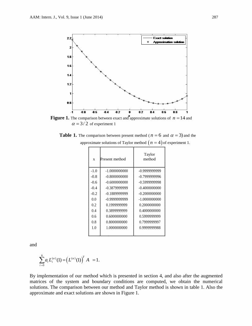
Figure 1. The comparison between exact and approximate solutions of 14n and

3/ 2 of experiment 1

Table 1. The comparison between present method ( 6n and 3) and the

approximate solutions of Taylor method 4n of experiment 1.

x Present method

Taylor

method

-1.0 -1.0000000000 -0.9999999999

-0.8 -0.8000000000 -0.7999999996

-0.6 -0.6000000000 -0.5999999998

-0.4 -0.3879999999 -0.4000000000

-0.2 -0.1889999999 -0.2000000000

0.0 -0.9999999999 -1.0000000000

0.2 0.1999999999 0.2000000000

0.4 0.3899999999 0.4000000000

0.6 0.6000000000 0.5999999999

0.8 0.8000000000 0.7999999997

1.0 1.0000000000 0.9999999988

and

6

( ) ( )

0

(1) (1) 1.T

i i

i

a L L A

By implementation of our method which is presented in section 4, and also after the augmented

matrices of the system and boundary conditions are computed, we obtain the numerical

solutions. The comparison between our method and Taylor method is shown in table 1. Also the

approximate and exact solutions are shown in Figure 1.


Experiment 2.

Consider the second-order linear differential equation:

2( 1) ( ) ( ) 1,x y x y x (34)

with the boundary conditions y(0)=0, y(1)=1.The exact solution of equation (34) is

( ) .y x x

Now we approximate the exact solution of equation (34), by

5

( ) ( )

0

( ) ( ) ( ) ,T

i i

i

y x a L x L x A

where 0 1 5A = [a ,a ,...,a ]. Also we expand the right hand side of equation (34) as

5

( ) ( )

0

1 ( ) ( ) ,T

i i

i

b L x L x B

where 1,0,0,0,0,0 .B

Now, first we reduce equation (34) into the following matrix form 2 2 2 .T

G D D D A B

Also its boundary conditions as

5

( ) ( )

0

(0) (0) 0,T

i i

i

a L L A

and

5

( ) ( )

0

(1) (1) 1.T

i i

i

a L L A

By implementation of our method which is presented in section 4, and also after the augmented

matrices of the system and boundary conditions are computed, we obtain the solution y(x)=x,

which is the exact solution.

Experiment 3.

Consider the third-order linear differential equation:

2 ( ) ( ) 2,x y x y x


y(0) = 0, y(1) = 1, y(-1)=1. (35)

Now we approximate the exact solution of equation (35) by

5

( ) ( )

0

( ) ( ) ( ) .T

i i

i

y x a L x L x A

Also we expand the right hand side of equation (35) as

5

( ) ( )

0

2 ( ) ( ) ,T

i i

i

b L x L x B

where [2,0,0,0,0,0].B

Now we must reduce equation (35) into the following matrix form

2 3 2 ,T

G D D A B

and also its boundary conditions as

5

( ) ( )

0

(0) (0) 0,T

i i

i

a L L A

5

( ) ( )

0

(1) (1) 1,T

i i

i

a L L A

and

5

( ) ( )

0

( 1) ( 1) 1.T

i i

i

a L L A

After the augmented matrices of the system and boundary conditions are computed, we obtain

the solution2( ) ,y x x which is the exact solution.

7. Application of the Method for the High-Order Linear Differential Equation

In this section, we report the numerical results obtained for a high-order linear differential

equation by the aforementioned procedure. This shows that it is straightforward to extend the

method to the high-order linear differential equations as follows.

Experiment 4.


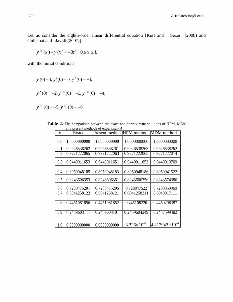
Let us consider the eighth-order linear differential equation [Kurt and Sezer (2008) and

Golbabai and Javidi (2007)]:

(8) ( ) ( ) 8 , 0 1,xy x y x e x

with the initial conditions

(4) (5)

(6) (7)

(0) 1, (0) 0, (0) 1,

(0) 2, (0) 3, (0) 4,

(0) 5, (0) 6.

y y y

y y y

y y

Table 2. The comparison between the exact and approximate solutions of HPM, MDM

and present methods of experiment 4 x Exact Present method HPM method MDM method

0.0 1.0000000000 1.0000000000 1.0000000000 1.0000000000

0.1 0.9946538262 0.9946538261 0.9946538263 0.9946538262 0.2 0.9771222065 0.9771222063 0.9771222065 0.9771222014

0.3 0.9449011653 0.9449011651 0.9449011653 0.9449010769

0.4 0.8950948185 0.8950948183 0.8950948186 0.8950941522

0.5 0.8243606353 0.8243606351 0.8243606356 0.8243574386

0.6 0.7288475201 0.7288475205 0.728847522 0.7288359969 0.7 0.6041258122 0.6041258121 0.6041258211 0.6040917111

0.8 0.4451081856 0.4451081852 0.445108220 0.4450208387

0.9 0.2459603111 0.2459603101 0.2459604249 0.2457599482

1.0 0.0000000000 0.0000000000 3.326710 4.212943

410



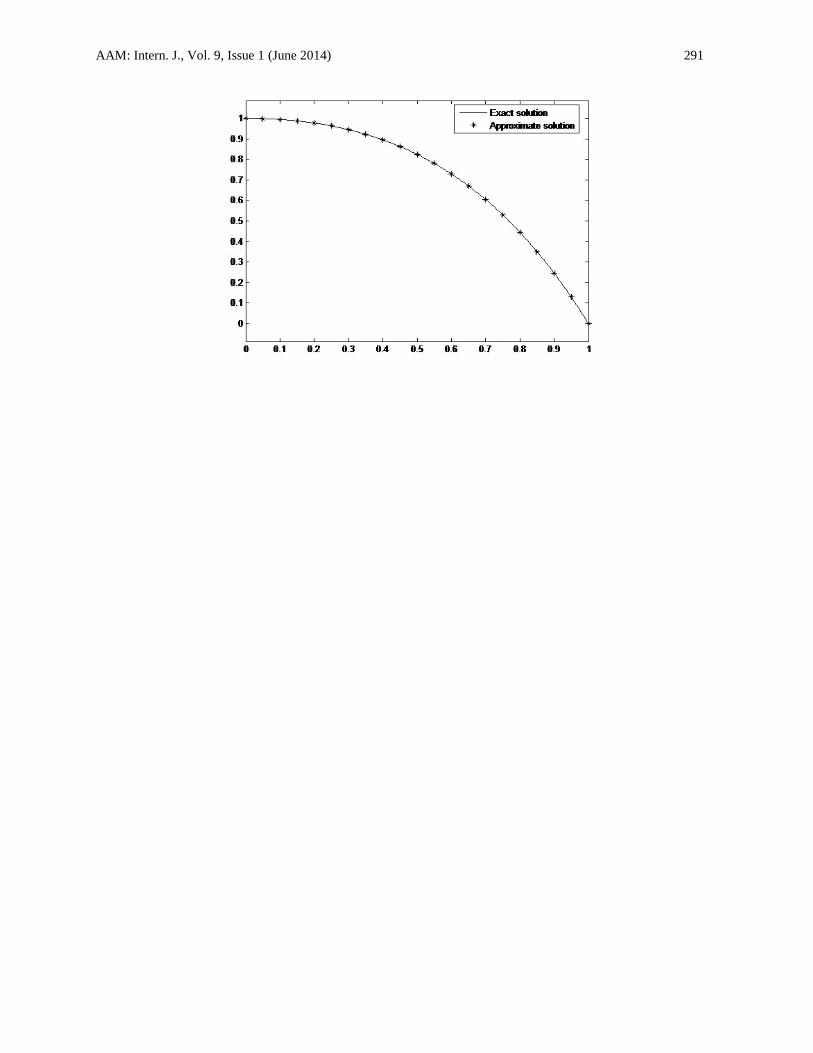
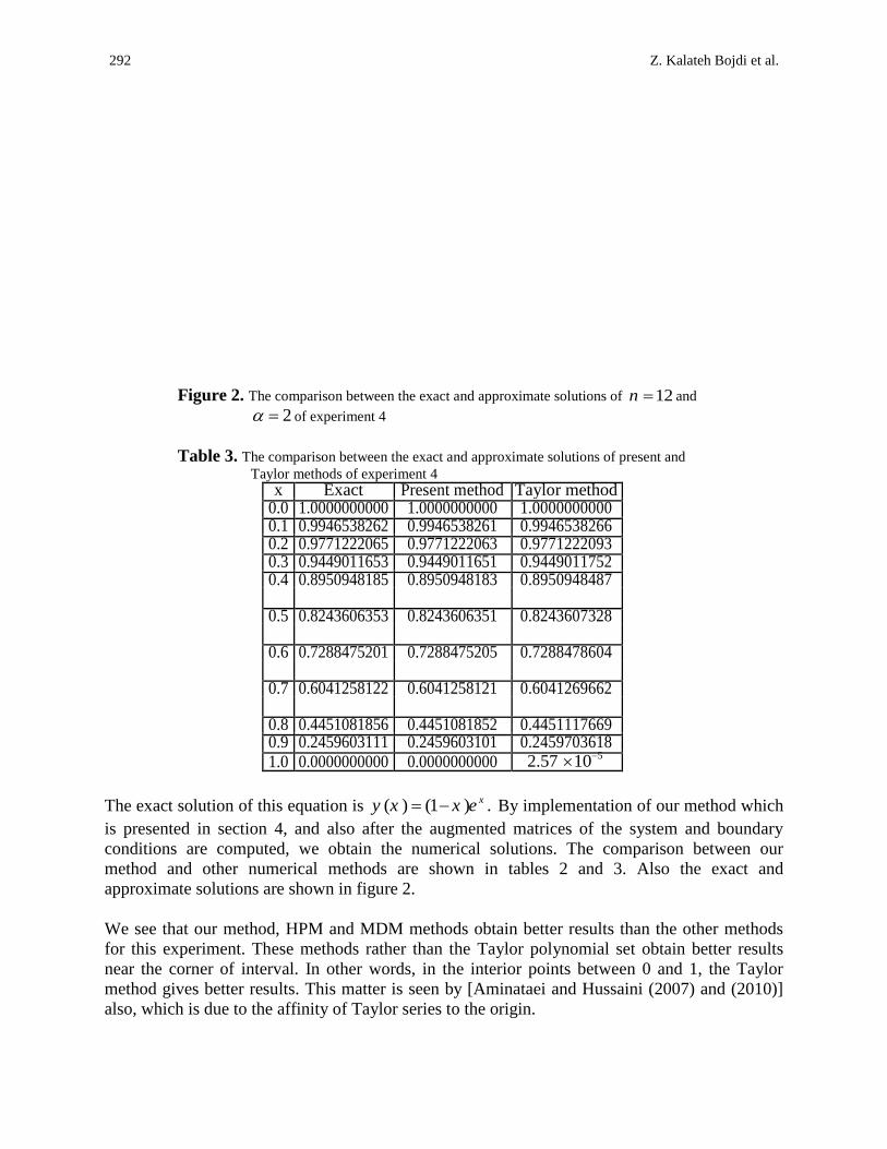
Figure 2. The comparison between the exact and approximate solutions of 12n and

2 of experiment 4

Table 3. The comparison between the exact and approximate solutions of present and

Taylor methods of experiment 4 x Exact Present method Taylor method

0.0 1.0000000000 1.0000000000 1.0000000000 0.1 0.9946538262 0.9946538261 0.9946538266 0.2 0.9771222065 0.9771222063 0.9771222093 0.3 0.9449011653 0.9449011651 0.9449011752 0.4 0.8950948185 0.8950948183 0.8950948487

0.5 0.8243606353 0.8243606351 0.8243607328

0.6 0.7288475201 0.7288475205 0.7288478604

0.7 0.6041258122 0.6041258121 0.6041269662

0.8 0.4451081856 0.4451081852 0.4451117669 0.9 0.2459603111 0.2459603101 0.2459703618 1.0 0.0000000000 0.0000000000 2.57

510

The exact solution of this equation is ( ) (1 ) .xy x x e By implementation of our method which

is presented in section 4, and also after the augmented matrices of the system and boundary

conditions are computed, we obtain the numerical solutions. The comparison between our

method and other numerical methods are shown in tables 2 and 3. Also the exact and

approximate solutions are shown in figure 2.

We see that our method, HPM and MDM methods obtain better results than the other methods

for this experiment. These methods rather than the Taylor polynomial set obtain better results

near the corner of interval. In other words, in the interior points between 0 and 1, the Taylor

method gives better results. This matter is seen by [Aminataei and Hussaini (2007) and (2010)]

also, which is due to the affinity of Taylor series to the origin.


8. Conclusion

In this paper, we have introduced a new and efficient approach for numerical approximation of

the linear differential-difference equations. The method is based on the approximation of the

exact solution with the generalized Laguerre polynomials approximation with variable

coefficients by Taylor series expansion. Implementation of the method reduces the problem to a

system of algebraic equations. Some test experiments are presented for showing the accuracy and

efficiency of the present method with the other methods such as HPM, MDM and Taylor series.

Application of the method for numerical solution of high-order linear differential equations is

also considered. In addition, we would like to emphasize that the main importance of the present

scheme is considering the general linear DDEs (1) and (2), whereas the other manuscripts only

considered the particular cases of our general problem. Further, using the generalized Laguerre

polynomials as the basis functions for numerical approximation whereas the classical Laguerre

polynomials are particular cases of them is another advantage of the present study.

Acknowledgments

We are grateful to the anonymous reviewers and the editor Professor Dr. Aliakbar Montazer

Haghighi for their helpful comments and suggestions which indeed improved the quality of this

manuscript.

REFERENCES

Agraval, R.P. and Oregan, D.O. (2009). Ordinary and Partial Differential Equations, Springer.

Akkaya, T. and Yalcinbas, S. (2012). Boubaker polynomial approach for solving high-order

linear differential-difference equations, AIP Conference Proceedings of 9th international

conference on mathematical problems in engineering, Vol. 56, pp. 26-33.

Aminataei, A. and Hussaini, S.S. (2007). The comparison of the stability of decomposition

method with numerical methods of equation solution, Appl. Math. Comput., Vol. 186, pp.

665-669.

Aminataei, A. and Hussaini, S.S. (2010). The barrier of decomposition method, Int. J. Contemp.

Math. Sci., Vol. 5, pp. 2487-2494.

Aminataei, A. and Vanani, S.K. (2013). Numerical solution of fractional Fokker-Planck equation

using the operational collocation method, Appl. Comput. Math., Vol. 12, pp. 33-43.

Askey, R. (1975). Orthogonal Polynomials and Special Functions. SIAM-CBMS, Philadelphia.

Ben-yu, G. (1996). The State of Art in Spectral Methods. Hong Kong University.

Boyd, J.P. (2000). Chebyshev and Fourier Spectral Methods. Dover Publications, Inc, New

York.

Canuto, C., Hussaini, M.Y., Quarteroni, A. and Zang, T.A. (1984). Spectral Method in Fluid

Dynamics, Prentice Hall, Engelwood Cliffs, NJ.

Canuto, C., Hussaini, M.Y., Quarteroni, A. and Zang, T.A. (2006). Spectral Methods:

Fundamentals in Single Domains, Springer-Verlag.

Danfu, H. and Xufeng, S. (2007). Numerical solution of integro-differential equations by using


CAS wavelet operational matrix of integration, Appl. Math. Comput., Vol. 194, pp. 460-466.

Dunkl, C.F. and Xu, Y. (2001). Orthogonal Polynomials of Several Variables, Cambridge

University Press.

Erdem, K. and Yalcinbas, S. (2012). Bernoulli polynomial approach to high-order linear diff-

erential-difference equations, AIP Conference Proceedings of Numerical Analysis and

Applied Mathematics, Vol. 73, pp. 360-364.

Eslahchi, M.R. and Dehghan, M. (2011). Application of Taylor series in obtaining the orthogonal

operational matrix, Computers and Mathematics with Applications, Vol. 61, pp. 2596-2604.

Funaro, D. (1992). Polynomial Approximations of Differential Equations, Springer-Verlag.

Gautschi, W. (2004). Orthogonal Polynomials (Computation and Approximation), Oxford

University Press.

Golbabai, A. and Javidi, M. (2007). Application of homotopy perturbation method for solving

eighth-order boundary value problems. Appl. Math. Comput., Vol. 213, pp. 203-214.

Gottlieb, D. and Orszag, S.A. (1977). Numerical Analysis of Spectral Methods: Theory and

Applica-tions. SIAM-CBMS, Philadelphia.

Gulsu, M. and Sezer, M. (2005). A method for the approximate solution of the high-order linear

difference equations in terms of Taylor polynomials, Int. J. Comput. Math., Vol. 82, pp.

629-642.

Gulsu, M. and Sezer, M. (2006). A Taylor polynomial approach for solving differential-

difference equa-tions, Comput. Appl. Math., Vol. 186, pp. 349-364.

Gulsu, M., Sezer, M. and Guney, Z. (2006). Approximate solution of general high-order linear

non-homogenous difference equations by means of Taylor collocation method, Appl. Math.

Comput., Vol. 173, pp. 683-693.

Hesthaven, J.S., Gottlieb, S. and Gottlieb, D. (2009). Spectral Methods for Time-Dependent

Problems. Cambridge University.

Hsiao, C. H. (2009). Hybrid function method for solving Fredholm and Volterra integral

equations of the second kind, Comput. Appl. Math., Vol. 230, pp. 59-68.

Imani, A., Aminataei, A. and Imani, A. (2011). Collocation method via Jacobi polynomials for

solving nonlinear ordinary differential equations, Int. J. Math. Math. Sci., Article ID

673085, 11P.

Kesan, C. (2003). Taylor polynomial solutions of linear differential equations, Appl. Math.

Comput., Vol. 142, pp. 155-165.

Khellat F. and Yousefi, S. A. (2006). The linear Legendre wavelets operational matrix of

integration and its application, J. Frank. Inst., Vol. 343, pp. 181-190.

King, A.C., Bilingham, J. and Otto, S.R. (2003). Differential Equations (Linear, Nonlinear,

Integral, Partial), Cambridge University.

Kurt, N. and Sezer, M. (2008). Polynomial solution of high-order linear Fredholm integro-diff-

erential equations with constant coefficients, J. Frank. Inst., Vol. 345, pp. 839-850.

Maleknejad, K. and Mirzaee, F. (2006). Numerical solution of integro-differential equations by

using rationalized Haar functions method, Kyber. Int. J. Syst. Math., Vol. 35, pp. 1735-1744.

Marcellan, F. and Assche, W.V. (2006). Orthogonal Polynomials and Special Functions (a

Computation and Applications), Springer-Verlag Berlin Heidelberg.

Ortiz, E. L. (1978). On the numerical solution of nonlinear and functional differential equations

with the Tau method, in: Numerical Treatment of Differential Equations in Applications, In:

Lecture Notes in Math., Vol. 679, pp. 127-139.

Ortiz, E. L. and Samara, L. (1981). An operational approach to the Tau method for the numer-


ical solution of nonlinear differential equations, Computing, Vol. 27, pp. 15-25.

Razzaghi, M. and Ordokhani, Y. (2001). Solution of nonlinear Volterra Hammerstein integral

equations via rationalized Haar functions, Math. Prob. Eng., Vol. 7, pp. 205-219.

Razzaghi, M. and Yousefi, S.A. (2005). Legendre wavelets method for the nonlinear Volterra-

Fredholm integral equations, Math. Comput. Simul., Vol. 70, pp. 1-8.

Reihani, M. H. and Abadi, Z. (2007). Rationalized Haar functions method for solving Fredholm

and Volterra integral equations, Comput. Appl. Math, Vol. 200, pp. 12-20.

Sezer, M. and Dascioglu, A.A. (2006). Taylor polynomial solutions of general linear differential-

difference equations with variable coefficients. Appl. Math. Comput., Vol. 174, pp. 1526-

1538.

Sezer, M. and Gulsu, M. (2005). Polynomial solution of the most general linear Fredholm

integro-differential-difference equation by means of Taylor matrix method, Int. J. Complex

Variables, Vol. 50, pp. 367-382.

Shen, J., Tang, T. and Wang, L.L. (2011). Spectral Methods Algorithms, Analysis and

Applications, Springer.

Trefethen, L.N. (2000). Spectral Methods in Matlab, SIAM, Philadelphia, PA.

Vanani, S. K. and Aminataei, A. (2012). A numerical algorithm for the space and time fractional

Fokker-Planck equation, Int. J. of Numer. Meth. for Heat & Fluid Flow, Vol. 22, pp. 1037-

1052.

Vanani, S.K. and Aminataei, A. (2011). Tau approximate solution of fractional partial

differential equations, Comput. Math. Appl., Vol. 62, pp. 1075-1083.

Wazwaz, A.M. (2010). The combined Laplace transform-Adomian decomposition method for

handling nonlinear Volterra integro-differential equations, Appl. Math. Comput., Vol. 216,

pp. 1304-1309.

Documents

The Generalized Laguerre Matrix Method or Solving Linear ... · The Generalized Laguerre Matrix Method or Solving Linear ... a new and efficient approach based on the generalized