Embed Size (px)
Citation preview

Computers and Chemical Engineering 29 (2005) 1891–1913
A cutting plane method for solving linear generalized disjunctiveprogramming problems
Nicolas W. Sawaya, Ignacio E. Grossmann∗
Department of Chemical Engineering, Carnegie Mellon University, Pittsburgh, PA 15213, USA
Received 19 April 2004; received in revised form 15 March 2005; accepted 5 April 2005Available online 2 June 2005
Abstract
Raman and Grossmann [Raman, R., & Grossmann, I.E. (1994). Modeling and computational techniques for logic based integer programming.Computers and Chemical Engineering, 18(7), 563–578] and Lee and Grossmann [Lee, S., & Grossmann, I.E. (2000). New algorithms fornonlinear generalized disjunctive programming.Computers and Chemical Engineering, 24, 2125–2141] have developed a reformulationof Generalized Disjunctive Programming (GDP) problems that is based on determining the convex hull of each disjunction. Although the
with thequires
n order tohod reliesm an LPelse untilng, retrofitutting plane
g
ndsi-
eci-
lento-kle
sesl al-lin-gh
this
relaxation of the reformulated problem using this method will often produce a significantly tighter lower bound when comparedtraditional big-M reformulation, the limitation of this method is that the representation of the convex hull of every disjunction rethe introduction of new disaggregated variables and additional constraints that can greatly increase the size of the problem. Icircumvent this issue, a cutting plane method that can be applied to linear GDP problems is proposed in this paper. The meton converting the GDP problem into an equivalent big-M reformulation that is successively strengthened by cuts generated froor QP separation problem. The sequence of problems is repeatedly solved, either until the optimal integer solution is found, orthere is no improvement within a specified tolerance, in which case one switches to a branch and bound method. The strip-packiplanning and zero-wait job-shop scheduling problems are presented as examples to illustrate the performance of the proposed cmethod.© 2005 Elsevier Ltd. All rights reserved.
PACS: 02.60.Pn
Keywords: MIP; Disjunctive Programming; Cutting planes; Mixed integer linear programming; Strip-packing; Retrofit planning; Job-shop schedulin
1. Introduction
The most commonly used model in discrete/continuousoptimization corresponds to a Mixed Integer Non LinearProgram (MINLP). More recently, however, GeneralizedDisjunctive Programming (GDP), which is a generaliza-tion of disjunctive programming (Balas, 1998), has beenproposed byRaman and Grossmann (1994)as an alter-native model to the MINLP problem (Grossmann, 2002;Tawarmalani & Sahinidis, 2002). While the MINLP modelis based entirely on algebraic equations and inequalities,
∗ Corresponding author. Tel.: +1 41 22683642; fax: +1 41 22687139.E-mail address: [email protected] (I.E. Grossmann).
the GDP model allows a combination of algebraic alogical equations through disjunctions and logic propotions, which facilitates the representation of discrete dsions. Furthermore,Lee and Grossmann (2000)have shownthat any GDP model can be converted into an equivaMINLP reformulation. Currently, there are several algrithms and different approaches in the literature to tacGDP problems (Grossmann, 2002), though some performinefficiently under certain conditions and for certain clasof problems. We are thus interested in developing novegorithms and solution methods aimed at solving bothear and non-linear GDP problems more efficiently, althouwe restrict ourselves exclusively to the linear case inpaper.
0098-1354/$ – see front matter © 2005 Elsevier Ltd. All rights reserved.doi:10.1016/j.compchemeng.2005.04.004
1892 N.W. Sawaya, I.E. Grossmann / Computers and Chemical Engineering 29 (2005) 1891–1913
Lee and Grossmann (2000)have proposed a reformula-tion to solve convex non-linear GDP problems with multipledisjunctions based on determining the convex hull of eachdisjunction. Although the feasible region of the reformulatedproblem does not correspond to the true convex hull of theproblem, we nonetheless have termed that reformulation inthis paper as the “convex hull” reformulation for the sakeof convenience. There exists other GDP to MINLP reformu-lations of which the traditional big-M reformulation is themost common.Grossmann and Lee (2003)have shown thatthe feasible region of the relaxation resulting from the con-vex hull reformulation projected onto the space of the big-Mreformulation is always as tight as, or tighter than that of thebig-M reformulation. The tightness of the relaxed feasibleregion, which is usually reflected in the lower bound of theproblem (for minimization), is an important criterion whensolving the original Mixed Integer Program, as tighter re-laxed feasible regions reduce the search space of the solutionalgorithm. However, the representation of the convex hull re-quires the introduction of new disaggregated variables andadditional constraints that can greatly increase the size of theproblem, thus limiting the effectiveness of the method.
In order to circumvent the aforementioned problem, wepresent in this paper a cutting plane method that exploits thepotentially tighter convex hull relaxed feasible region withoutthe additional constraints and variables. This method can be
b-tion
aitnalob-on-
ng
Here,x is a vector of continuous variables bounded bya vector of upper boundsU, Yjk are Boolean variables,ck ∈R1+ are continuous variables that represent the cost as-sociated with each disjunction andγ jk are fixed charges.A disjunction k∈K is composed of several disjunctsj∈Jk,each containing a set of linear equations and/or inequali-ties (Ajkx ≤ ajk) representing the constraints of the problem,connected together by the logical OR operator (∨) that en-forces the contents of only one disjunct. Discrete decisionsare represented by the Boolean variablesYjk in terms ofdisjunctionsk∈K and logic propositionsΩ(Y) that are as-sumed to be expressed in Conjunctive Normal Form (CNF).Thus, only the constraints inside disjunctj∈Jk, whereYjk istrue, are enforced; otherwise, the corresponding constraintsare not enforced. Finally,Bx ≤ b are common constraintsthat must hold regardless of the discrete decisions that areselected.
The linear GDP problem (LGDP) can be reformulated asa Mixed Integer Program (MIP) in different ways, includingthe two most common alternatives termed big-M (BM) andconvex hull reformulations (CH). In order to obtain the big-M reformulation, problem LGDP is transformed into an MIPby replacing the Boolean variablesYjk by binary variablesyjk and using big-M constraints. The logic constraintsΩ(Y)are converted into linear inequalities (Williams, 1985), whichleads to the following reformulation (Raman & Grossmann,1
s ny -tc 4)a
H),p ac-ian tsf n,1
applied to linear GDP problems that correspond to MIP prolems, or else to master problems that are used in the soluof non-linear GDP problems (Turkay & Grossmann, 1996).We present the strip-packing, retrofit planning and zero-wjob-shop scheduling problems to illustrate the computatioperformance of the proposed method in solving these prlems and compare all results obtained to those using the cvex hull and big-M reformulations.
2. Background
Consider the linear generalized disjunctive programmiproblem (LGDP), which is based on the work ofRaman andGrossmann (1994)and is an extension of the work ofBalas(1998):
Min Z =∑
∀k ∈ K
ck + dTx
s.t. Bx ≤ b
∨∀j ∈ Jk
Yjk
Ajkx ≤ ajk
ck = γjk
∀k ∈ K
Ω(Y ) = True
0 ≤ x ≤ U, ck ∈R1+, Yjk ∈ True, False ∀j ∈ Jk, ∀k ∈ K
(LGDP)
994):
Min Z =∑
∀k ∈ K
∑∀j ∈ Jk
γjkyjk + dTx
s.t. Bx ≤ b
Ajkx − ajk ≤ Mjk(1 − yjk) ∀j ∈ Jk, ∀k ∈ K∑∀j ∈ Jk
yjk = 1 ∀k ∈ K
Dy ≤ d
x ∈Rn+, yjk ∈ 0, 1 ∀j ∈ Jk, ∀k ∈ K(BM)
Here,Mjk are the “big-M” parameters that render thejthystem of inequalities in thekth disjunction redundant whejk = 0 (i.e.Yjk = False). The inequalitiesDy ≤ d can be sysematically derived from their logical CNF formΩ(Y) as dis-ussed byWilliams (1985), Raman and Grossmann (199,ndHooker (2000).
In order to obtain the convex hull reformulation (Croblem LGDP is transformed into an MIP by repl
ng the Boolean variablesYjk by binary variablesyjknd disaggregating the continuous variablesx ∈Rn+ intoew variablesν ∈Rn+. Using the convex hull constrain
or each disjunction (Balas, 1998; Raman & Grossman994), this leads to the following reformulation (Raman &
N.W. Sawaya, I.E. Grossmann / Computers and Chemical Engineering 29 (2005) 1891–1913 1893
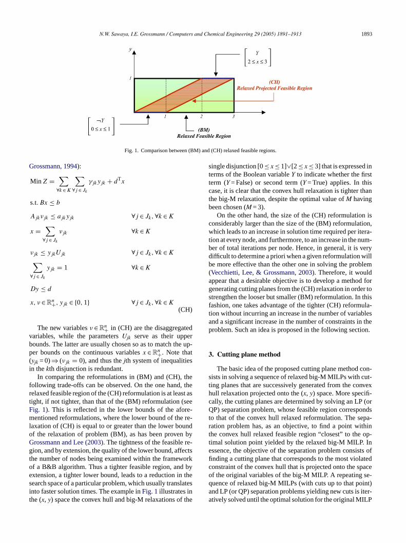
Fig. 1. Comparison between (BM) and (CH) relaxed feasible regions.
Grossmann, 1994):
Min Z =∑
∀k ∈ K
∑∀j ∈ Jk
γjkyjk + dTx
s.t. Bx ≤ b
Ajkνjk ≤ ajkyjk ∀j ∈ Jk, ∀k ∈ K
x =∑
∀j ∈ Jk
νjk ∀k ∈ K
νjk ≤ yjkUjk ∀j ∈ Jk, ∀k ∈ K∑∀j ∈ Jk
yjk = 1 ∀k ∈ K
Dy ≤ d
x, ν ∈Rn+, yjk ∈ 0, 1 ∀j ∈ Jk, ∀k ∈ K(CH)
The new variablesν ∈Rn+ in (CH) are the disaggregatedvariables, while the parametersUjk serve as their upperbounds. The latter are usually chosen so as to match the up-per bounds on the continuous variablesx ∈Rn+. Note that(yjk = 0)⇒ (νjk = 0), and thus thejth system of inequalitiesin thekth disjunction is redundant.
etht aee-rendby-ctory
thte
he
single disjunction [0≤ x ≤ 1]∨[2 ≤ x ≤ 3] that is expressed interms of the Boolean variableY to indicate whether the firstterm (Y = False) or second term (Y = True) applies. In thiscase, it is clear that the convex hull relaxation is tighter thanthe big-M relaxation, despite the optimal value ofM havingbeen chosen (M = 3).
On the other hand, the size of the (CH) reformulation isconsiderably larger than the size of the (BM) reformulation,which leads to an increase in solution time required per itera-tion at every node, and furthermore, to an increase in the num-ber of total iterations per node. Hence, in general, it is verydifficult to determine a priori when a given reformulation willbe more effective than the other one in solving the problem(Vecchietti, Lee, & Grossmann, 2003). Therefore, it wouldappear that a desirable objective is to develop a method forgenerating cutting planes from the (CH) relaxation in order tostrengthen the looser but smaller (BM) reformulation. In thisfashion, one takes advantage of the tighter (CH) reformula-tion without incurring an increase in the number of variablesand a significant increase in the number of constraints in theproblem. Such an idea is proposed in the following section.
3. Cutting plane method
The basic idea of the proposed cutting plane method con-t-vex
orndsa-in-
s ofedce-)r-
In comparing the reformulations in (BM) and (CH), thfollowing trade-offs can be observed. On the one hand,relaxed feasible region of the (CH) reformulation is at leastight, if not tighter, than that of the (BM) reformulation (seFig. 1). This is reflected in the lower bounds of the aformentioned reformulations, where the lower bound of thelaxation of (CH) is equal to or greater than the lower bouof the relaxation of problem (BM), as has been provenGrossmann and Lee (2003). The tightness of the feasible region, and by extension, the quality of the lower bound, affethe number of nodes being examined within the framewof a B&B algorithm. Thus a tighter feasible region, and bextension, a tighter lower bound, leads to a reduction insearch space of a particular problem, which usually translainto faster solution times. The example inFig. 1illustrates inthe (x, y) space the convex hull and big-M relaxations of t
es
-
sk
es
sists in solving a sequence of relaxed big-M MILPs with cuting planes that are successively generated from the conhull relaxation projected onto the (x, y) space. More specifi-cally, the cutting planes are determined by solving an LP (QP) separation problem, whose feasible region correspoto that of the convex hull relaxed reformulation. The sepration problem has, as an objective, to find a point withthe convex hull relaxed feasible region “closest” to the optimal solution point yielded by the relaxed big-M MILP. Inessence, the objective of the separation problem consistfinding a cutting plane that corresponds to the most violatconstraint of the convex hull that is projected onto the spaof the original variables of the big-M MILP. A repeating sequence of relaxed big-M MILPs (with cuts up to that pointand LP (or QP) separation problems yielding new cuts is iteatively solved until the optimal solution for the original MILP
1894 N.W. Sawaya, I.E. Grossmann / Computers and Chemical Engineering 29 (2005) 1891–1913
is found or until there is no improvement within a specifiedtoleranceε, in which case one switches to a B&B method forsolving the resulting big-M MILP with all the cutting planesthat have been generated.
It is interesting to note that the proposed cuts, though re-lated to a certain extent to some of the work done on lift-and-project cutting planes originally developed byBalas, Ceria,and Cornuejols(1993), are different in important ways fromthe latter. The major distinction lies in the derivation and gen-eration of our cuts, which are crucially based on a GDP for-mulation, as opposed to a 0–1 MIP formulation, as in the caseof lift-and-project cuts. Furthermore, if we were to contex-tualize their work within a GDP framework, lift-and-projectcuts would be generated through a sequential convexificationprocedure that would obtain by taking the convex hull of onedisjunction at a time, as opposed to our proposed methodwhich generates cuts based on a formulation that considersthe intersection of the convex hulls of every disjunction. Thus,the elementary closure resulting from our cuts is not equiva-lent to that of lift-and-project cuts, since the latter’s closurecorresponds to the true convex hull of the original problem,as opposed to our case, where the elementary closure cor-responds to the feasible region arising from the aforemen-tioned strengthened formulation that considers all disjunc-tions simultaneously. We plan on comparing our cuts, both
e-rs
l-
the Euclidean norm,φ(z) = ||z − zbm||2 ≡ [(z − zbm)T
(z − zbm)]1/2,or the infinity norm,φ(z) = ||z − zbm||∞ ≡ maxi|zi − zbm
i |can be used. If either the 1-norm or the∞-norm is used,then the separation problem is an LP; otherwise, using theEuclidean norm yields a QP.
3.2. Derivation of cutting planes
In this section, we present the derivation of the proposedcutting planes that are obtained from the separation problem(SEP). The proofs of the propositions presented can be foundin Appendix A.
The first proposition formalizes the observation inFig. 1that the feasible region of the separation problem (SEP),which corresponds to that of the convex hull reformulation,is contained within the feasible region of problem (BM).
Proposition 1. Let (FR-SEP) be the feasible region of theseparation problem (SEP) in the (z, ν) space, and let (FRP-SEP) represent the projection of (FR-SEP) onto the z-space.Then, (FRP-SEP)⊆(FR-BM), where (FR-BM) represents thefeasible region of (BM) in the z-space. Furthermore, (FRP-SEP) is a convex set.
thet is
),cutsible
dif-gra-
ions
at
theoretically and computationally, to other cuts present in thliterature, including lift-and-project cuts, mixed-integer Gomory cuts and mixed-integer rounding cuts, amongst othein a subsequent paper.
3.1. Separation problem
The general form of the separation problem (SEP) is as folows (seeStubbs & Mehrotra, 1999; Vecchietti et al., 2003):
Min φ(z) = ||z − zbm||s.t. Bx ≤ b
Ajkνjk ≤ ajkyjk ∀j ∈ Jk, ∀k ∈ K
x =∑
∀j ∈ Jk
νjk ∀k ∈ K
νjk ≤ yjkUjk ∀j ∈ Jk, ∀k ∈ K∑∀j ∈ Jk
yjk = 1 ∀k ∈ K
Dy ≤ d
x, ν ∈Rn+, z ≡ [x, y] ∈Rn+×R
∑∀k ∈ K
|Jk |+ , 0 ≤ yjk ≤ 1 ∀j ∈ Jk, ∀k ∈ K
(SEP)
The objective functionφ(z) corresponds to determiningthe pointz ∈Rn+ × R
∑∀k ∈ K
|Jk |+ within the convex hull relax-ation “closest” to the pointzbm, which corresponds to theoptimal solution of the relaxed big-M MILP. In order to rep-resent distance in the functionφ(z),
the 1-norm,φ(z) = ||z − zbm||1 ≡ ∑i |zi − zbm
i |,
,
The second proposition provides the general form ofvalid inequality that corresponds to the cutting plane thadetermined from the separation problem (SEP).
Proposition 2. Let zbm be the optimal solution of (BM) andzsepbe an optimal solution to (SEP). If zbm/∈(FRP-SEP), then∃ξ such that ξT(z − zsep) ≥ 0 is a valid linear inequality in zthat cuts away zbm, and such that ξ is a subgradient of φ(z)at zsep, where φ(z) corresponds to the objective function of(SEP).
Using the example previously shown inFig. 1, Fig. 2demonstrates how the proposed cutξT(z − zsep) ≥ 0 cuts awayzbm and slices off part of the feasible region of problem (BMthus strengthening the formulation. Also, note that thegenerated in this case corresponds to a facet of the fearegion of problem (SEP).
The third proposition shows that the subgradient of aferentiable function at a specific point corresponds to thedient of the function at that same point.
Proposition 3. Let (FRP-SEP)⊂S, where S is a convex set.If φ : S → R is differentiable over its entire domain, thenthe collection of subgradients of φ at zsep is the singletonset ∂sepφ ≡ ξsep|ξsep= ∇φ(zsep), which corresponds to thegradient of φ at zsep.
The last two propositions provide the specific expressfor the subgradientξ in the inequalityξT(z − zsep) ≥ 0 for theEuclidean and∞-norms, respectively. It should be noted th

N.W. Sawaya, I.E. Grossmann / Computers and Chemical Engineering 29 (2005) 1891–1913 1895
Fig. 2. Graphical representation ofProposition 2.
for the case of the 1-norm, the treatment is entirely similar asthe∞-norm.
Proposition 4. Let (FRP-SEP)⊂S, where S is a convexset. If φ : S → R is defined as φ(z) = ||z − zbm||22, then thecollection of subgradients of φ at zsep is the singleton set∂sepφ ≡ ξsep|ξsep= 2(zsep− zbm).
Proposition 5. Let (FRP-SEP)⊂S, where S is a convex set.If φ : S → R is defined as φ(z) = ||z − zbm||∞, then the col-lection of subgradients of φ at zsep is the set:
∂sepφ ≡ ξsep|ξsep= [µsep+ − µ
sep− ]
where µsep+ and µ
sep− correspond to the optimal Lagrange
multipliers of constraints (1) and (2) respectively, in the fol-lowing problem (SEP2):
Min u
s.t. u ≥ zi − zbmi ∀i ∈ M (1)
u ≥ zbmi − zi ∀i ∈ M (2)
R1z + R2ν ≤ r
The cutting planes generated by the proposed method andbased onPropositions 2, 4 and 5can be used at the rootnode of the branch and bound tree in order to strengthen thecorresponding relaxation of problem (BM). It is, of course,generally not obvious which of the different norms pro-vides the deepest cut, as this is usually problem depen-dent. Furthermore, the depth of the cut will be affected,particularly in the cases of the 1-norm and the∞-norm,by the selection of a specific set of (non-unique) optimalLagrange multipliers, which is usually solver dependent.The following example provides a geometrical interpretationof the three different cuts when applied to the example inFig. 1.
MaxZ = x − (c1 + c2)
s.t.
Y
2 ≤ x ≤ 3
c1 = 1
∨
¬Y
0 ≤ x ≤ 1
c2 = 0
In Fig. 3, the cut generated when the Euclidean norm orinfinity norm is used corresponds to a facet of the convex
E
Fig. 3. Cutting plane generated when uclidean or infinity norm are used in (SEP).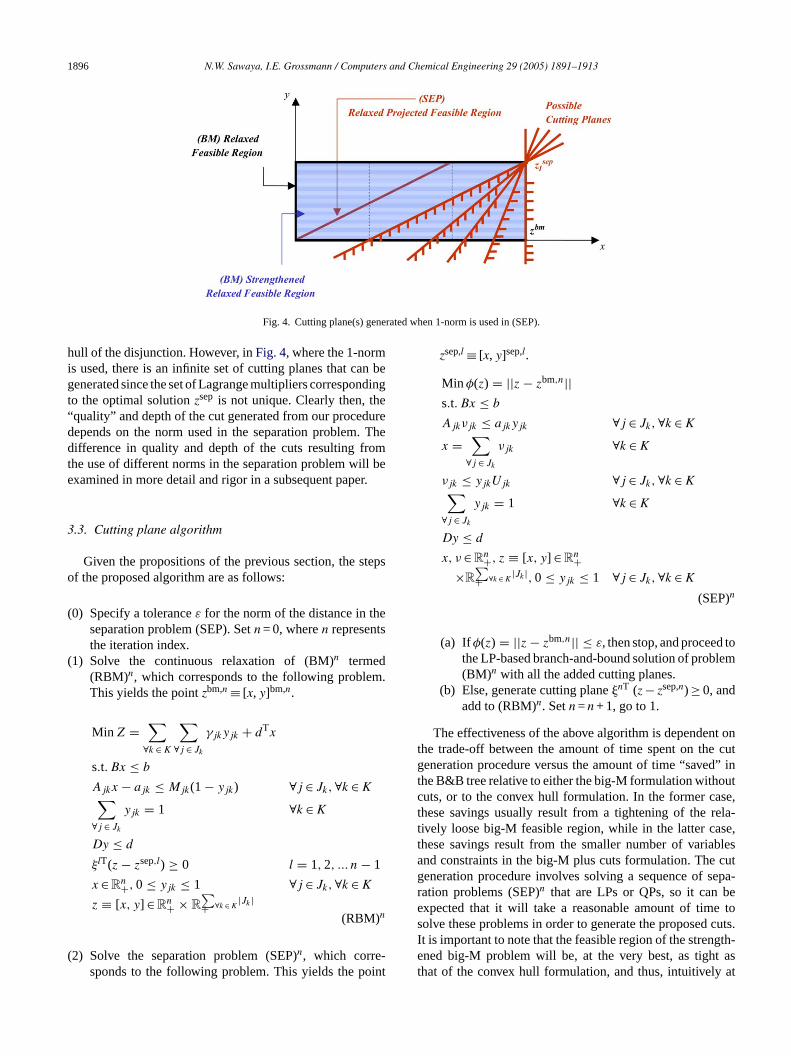
1896 N.W. Sawaya, I.E. Grossmann / Computers and Chemical Engineering 29 (2005) 1891–1913
Fig. 4. Cutting plane(s) generated when 1-norm is used in (SEP).
hull of the disjunction. However, inFig. 4, where the 1-normis used, there is an infinite set of cutting planes that can begenerated since the set of Lagrange multipliers correspondingto the optimal solutionzsep is not unique. Clearly then, the“quality” and depth of the cut generated from our proceduredepends on the norm used in the separation problem. Thedifference in quality and depth of the cuts resulting fromthe use of different norms in the separation problem will beexamined in more detail and rigor in a subsequent paper.
3.3. Cutting plane algorithm
Given the propositions of the previous section, the stepsof the proposed algorithm are as follows:
(0) Specify a toleranceε for the norm of the distance in theseparation problem (SEP). Setn = 0, wheren representsthe iteration index.
(1) Solve the continuous relaxation of (BM)n termed(RBM)n, which corresponds to the following problem.This yields the pointzbm,n ≡ [x, y]bm,n.
Min Z =∑ ∑
γjkyjk + dTx
nt
zsep,l ≡ [x, y]sep,l.
Min φ(z) = ||z − zbm,n||s.t. Bx ≤ b
Ajkνjk ≤ ajkyjk ∀j ∈ Jk, ∀k ∈ K
x =∑
∀j ∈ Jk
νjk ∀k ∈ K
νjk ≤ yjkUjk ∀j ∈ Jk, ∀k ∈ K∑∀j ∈ Jk
yjk = 1 ∀k ∈ K
Dy ≤ d
x, ν ∈Rn+, z ≡ [x, y] ∈Rn+×R
∑∀k ∈ K
|Jk |+ , 0 ≤ yjk ≤ 1 ∀j ∈ Jk, ∀k ∈ K
(SEP)n
(a) If φ(z) = ||z − zbm,n|| ≤ ε, then stop, and proceed tothe LP-based branch-and-bound solution of problem(BM)n with all the added cutting planes.
(b) Else, generate cutting planenT (z − zsep,n) ≥ 0, andadd to (RBM)n. Setn = n + 1, go to 1.
The effectiveness of the above algorithm is dependent onutin
te,a-,
lesutpa-
touts.h-st
∀k ∈ K ∀j ∈ Jk
s.t. Bx ≤ b
Ajkx − ajk ≤ Mjk(1 − yjk) ∀j ∈ Jk, ∀k ∈ K∑∀j ∈ Jk
yjk = 1 ∀k ∈ K
Dy ≤ d
ξlT(z − zsep,l) ≥ 0 l = 1, 2, ... n − 1
x ∈Rn+, 0 ≤ yjk ≤ 1 ∀j ∈ Jk, ∀k ∈ K
z ≡ [x, y] ∈Rn+ × R∑
∀k ∈ K|Jk |+
(RBM)n
(2) Solve the separation problem (SEP)n, which corre-sponds to the following problem. This yields the poi
the trade-off between the amount of time spent on the cgeneration procedure versus the amount of time “saved”the B&B tree relative to either the big-M formulation withoucuts, or to the convex hull formulation. In the former casthese savings usually result from a tightening of the reltively loose big-M feasible region, while in the latter casethese savings result from the smaller number of variaband constraints in the big-M plus cuts formulation. The cgeneration procedure involves solving a sequence of seration problems (SEP)n that are LPs or QPs, so it can beexpected that it will take a reasonable amount of timesolve these problems in order to generate the proposed cIt is important to note that the feasible region of the strengtened big-M problem will be, at the very best, as tight athat of the convex hull formulation, and thus, intuitively a
N.W. Sawaya, I.E. Grossmann / Computers and Chemical Engineering 29 (2005) 1891–1913 1897
least, lead us to believe that the cut generation procedureis finite. In other words, no further cuts will be generatedeither when the optimal point of (RBM)n lies within the fea-sible region of (SEP)n, or when the feasible region of thestrengthened big-M problem is exactly equivalent to that of(SEP)n. A rigorous proof of the previous claim will be per-formed in a subsequent paper. The question that remains,however, is whether these cuts are effective enough in slicingoff parts of the big-M feasible region that are superfluous.This is examined in detail in the next section, and we applythe above algorithm to three different problems that highlightsome of the major strengths and weaknesses of the proposedmethod.
4. Numerical results
In this section, we present the results of the proposedcutting plane algorithm on the strip-packing, retrofit plan-ning and zero-wait job-shop scheduling problems. The strip-packing problem is an example within a class of problemssuitably solved by the proposed method, while the last twoproblems serve to highlight an important characteristic re-garding the usefulness of the method, notably the degree oftightness exhibited by the convex hull relaxation.
thn
hiroen
afop
al
sorp-heeatheeffiro
wnatu
ng
problem, where a given set of small rectangles is packed intoa strip of fixed widthW but unknown lengthL. The aim isto minimize the length of the strip while fitting all rectangleswithout any overlap and without rotation. We propose thefollowing general linear GDP model for problem (SP-GDP):
Min lt (1)
s.t. lt ≥ xi + Li ∀i ∈ N (2)
[Y1
ij
xi + Li ≤ xj
]∨
[Y2
ij
xj + Lj ≤ xi
]∨
[Y3
ij
yi − Hi ≥ yj
]
∨[
Y4ij
yj − Hj ≥ yi
]∀i, j ∈ N, i < j (3)
xi ≤ UBi − Li ∀i ∈ N (4)
Hi ≤ yi ≤ W ∀i ∈ N (5)
lt, xi, yi ∈R1+, Y1
ij, Y2ij, Y
3ij, Y
4ij ∈ True, False
∀i, j ∈ N, i < j
The objective in this problem consists of minimizing the
ry
esct
d
d
per
p-d(3,),y
re-
We present results for the strip-packing problem usingproposed method with all norms, although the discussiomostly focused on results obtained using theinfinity normas the latter turned out to be the most efficient norm. Tobservation also holds true for the retrofit planning and zewait job-shop scheduling problems, thus, we only presand discuss results obtained using theinfinity norm. All re-sults obtained using the proposed cutting plane methoddiscussed and compared with those obtained using the amentioned convex hull and big-M reformulations, where otimal values of the big-M parameters were used (i.e. equmaxx(Ajkx − ajk)).
All example problems were solved with GAMS (Brooke,Kendrick, Meeraus, & Raman, 1997) on a 2.8 GHz PentiumIV PC (512 MB of RAM). The CPLEX solver (v. 8.1) waused for the infinity norm for all three problems and fall comparisons between reformulations with all MIP otions turned off and with default options turned on, while tCPLEX solver (v. 9.0) was used for the 1-norm and Euclidnorm. Note that the LP pre-solver was turned off duringcut-generation procedure for reasons of computationalciency. Finally, the cuts generated are added only at thenode of the B&B tree.
4.1. Strip-packing problem
Cutting and packing problems belong to a well-knofamily of combinatorial NP-hard optimization problems tharise in numerous applications of computer science, indtrial engineering, and operations management (Hifi, 1998).One important problem in this family is the strip-packi
eis
s-t
rere--to
n
-ot
s-
length of the striplt (1)and(2)by representing every rectangleby its coordinates in the (x, y) space such that no overlapoccurs between rectangles. Thus, every rectanglei∈N haslengthLi, heightHi, and coordinates (xi, yi), where the pointof reference corresponds to the upper left corner of everectangle. By constraining every pair of rectangles (i, j) where(i, j∈N, i < j) such that no overlap occurs, we obtain a seriof disjunctions with four disjuncts each, where each disjunrepresents the position of rectanglei in relation to rectanglej(3). Note that they-coordinate of every rectangle is boundefrom above by the fixed width of the stripW (5), and thatthe upper boundUBi, which in a best case scenario woulcorrespond to the optimal value oflt, is obtained using abottom-left rectangle-placing heuristic and serves as an upbound for thex-coordinate of every rectangle(4).
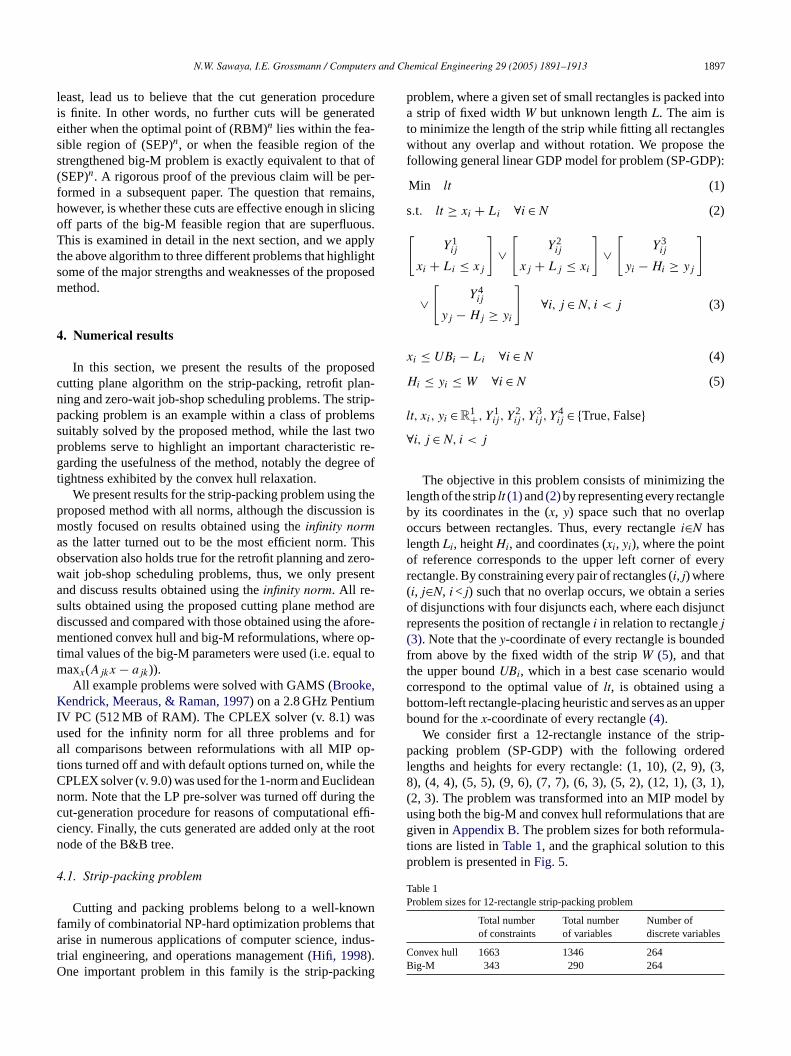
We consider first a 12-rectangle instance of the stripacking problem (SP-GDP) with the following orderelengths and heights for every rectangle: (1, 10), (2, 9),8), (4, 4), (5, 5), (9, 6), (7, 7), (6, 3), (5, 2), (12, 1), (3, 1(2, 3). The problem was transformed into an MIP model busing both the big-M and convex hull reformulations that agiven inAppendix B. The problem sizes for both reformulations are listed inTable 1, and the graphical solution to thisproblem is presented inFig. 5.
Table 1Problem sizes for 12-rectangle strip-packing problem
Total numberof constraints
Total numberof variables
Number ofdiscrete variables
Convex hull 1663 1346 264Big-M 343 290 264

1898 N.W. Sawaya, I.E. Grossmann / Computers and Chemical Engineering 29 (2005) 1891–1913
Fig. 5. Graphical solution for 12-rectangle strip-packing problem.
Table 2Results for 12-rectangle strip-packing problem (∞-norm, MIP options off)
Relaxation Optimalsolution
Gap (%) Total nodesin MIP
Solution time forcut generation (s)
Total solutiontimea (s)
Number of nodesper second
Convex hull 12 27 55.55 682464 0 1286.39 530.52Big-M 12 – – 54244296 0 >10800 5022.36Big-M + 40 cuts 12 – – 41831856 2.44 >10800 3873.32Big-M + 50 cuts 12 27 55.55 10289250 3.05 2986.33 3448.97Big-M + 60 cuts 12 27 55.55 694596 3.66 191.95 3688.96Big-M + 70 cuts 12 27 55.55 320535 4.27 97.61 3434.05Big-M + 80 cuts 12 27 55.55 502727 4.88 154.23 3366.09Big-M + 87 cuts 12 27 55.55 72677 5.31 27.51 3273.73
a Total solution time includes times for relaxed MIP(s) + LP(s) from separation problem + MIP.
We also solved the problem using the cutting plane methodwith the infinity norm, and compared the resulting solutionsto those from the convex hull and big-M reformulations inTables 2 and 3. We first examine the results with all MIPalgorithmic options turned off (seeTable 2). This is donein order to better gauge the effect of the proposed cuts onsolution time and number of nodes examined during the B&Bprocedure.
The optimal solution of the problem is 27. The lowerbound obtained from the relaxation is equal to 12 for both(BM) and (CH) reformulations, but the problem was solvedin 682 464 nodes using the (CH) reformulation, as opposedto the big-M reformulation, which failed to solve the prob-
lem after 54 244 296 nodes. This is due to the tighter relaxedfeasible region of (CH) when compared to that of (BM),which results in substantial savings in computational time(1286.39 s versus >10 800 s). Note however that the LP atevery node of the (CH) B&B tree is about 10 times more ex-pensive to solve than that of the (BM) reformulation as seenby the amount of nodes computed per second for both refor-mulations (530.52 versus 5022.36). This is due to the largernumber of variables and constraints present in the (CH) refor-mulation. After the addition of 50 cutting planes to the (BM)reformulation, we are able to solve the problem in less thanthe self-imposed limit of 3 h (2986.33 s) while examining10 289 250 nodes in the B&B tree. Upon the successive ad-
Table 3Results for 12-rectangle strip-packing problem (∞-norm, default options on)
Relaxation Optimalsolution
Gap (%) Total nodesin MIP
Solution time forcut generation (s)
Total solutiontimea (s)
Number of nodesper second
Convex hull 12 – – 2887380 0 >10800 267.35Big-M 12 27 55.55 73225 0 59.00 1241.10Big-M + 40 cuts 12 27 55.55 13361 2.44 12.21 1368.25Big-M + 50 cuts 12 27 55.55 9008 3.05 11.01 1131.65Big-M + 60 cuts 12 27 55.55 20247 3.66 20.61 1194.51Big-M + 70 cuts 12 27 55.55 11405 4.27 14.05 1166.15Big-M + 80 cuts 12 27 55.55 10225 4.88 14.41 1072.92Big-M + 87 cuts 12 27 55.55 6397 5.31 11.12 1101.03
eparat
a Total solution time includes times for relaxed MIP(s) + LP(s) from s ion problem + MIP.
N.W. Sawaya, I.E. Grossmann / Computers and Chemical Engineering 29 (2005) 1891–1913 1899
Table 4Results for 12-rectangle strip-packing problem (1-norm, MIP options off)
Relaxation Optimalsolution
Gap (%) Total nodesin MIP
Solution time forcut generation (s)
Total solutiontimea (s)
Number of nodesper second
Convex hull 12 27 55.55 682464 0 1286.39 530.52Big-M 12 – – 54244296 0 >10800 5022.36Big-M + 50 cuts 12 – – 17145216 6.0 >10800 1587.52Big-M + 100 cuts 12 – – 7373700 12.0 >10800 682.75Big-M + 200 cuts 12 – – 253800 22.0 >10800 23.5
a Total solution time includes times for relaxed MIP(s) + LP(s) from separation problem + MIP.
dition of more cuts, the number of nodes examined is furtherreduced, which results in a further decrease in total solutiontime. Finally, with 87 cuts, the proposed cutting plane algo-rithm solves this problem in 72 677 nodes. Although the re-sulting strengthened MIP is still not as tight as the (CH) MIP,it has much fewer variables. This compromise is key to thesuccess of the proposed algorithm and results in improved to-tal computational times (27.51 s versus 1286.39 s). Note thatthe time required to generate the 87 cutting planes was only5.31 s.
We now examine the results with default options turnedon. This is done in order to demonstrate the effectiveness ofthe proposed cuts in aiding the branch-and-cut routine of apowerful MIP solver like CPLEX (seeTable 3).
We see a noticeable improvement in the number of nodesexamined and solution times upon the addition of the cuts.After 87 cuts, the problem was solved in 6397 nodes and11.12 s compared to 73 225 nodes and 59.00 s for the big-M.However, CPLEX failed to solve the CH reformulation inless than 3 h, which is odd considering that one would expectan improvement in nodes examined and solution times whendefault options are turned on. This phenomenon could havebeen caused by many factors, although we believe that poorCPLEX-generated cuts are the most likely culprits. As moreCPLEX cuts are generated, they tend to become shallowerand to flatten out, and upon their addition to the matrix of thep ningn ies.T the-l uttingp op-t lemw
he 1-n
used. Note that while the use of the 1-norm in problem (SEP)still results in an LP, the use of the Euclidean norm results ina QP. Also, only results obtained with all MIP options turnedoff are presented.
Using the 1-norm or the Euclidean norm for the objec-tive function in the separation problem does not yield goodresults as CPLEX failed to solve the problem to optimality.Furthermore, and in both cases, the cut generation routinewas terminated after the self-imposed limit of 200 cuts with-out having reduced the objective function value to zero inthe separation problem. The problem in both cases is thatthe cuts generated are weak and do not tighten the feasibleregion enough. Moreover, upon the addition of more cuts inthe hope of strengthening the formulation and improving so-lution times, we observe the same phenomenon that occurredwhen we attempted to solve the convex hull formulation withdefault MIP options on. In other words, the addition of moreof these “poor” cuts negatively affects the computational per-formance of the algorithm because of numerical difficulties.In light of these observations in this case and other cases,we will only report results using the infinity norm for theremainder of this paper.
Let us now consider a 21-rectangle instance of the strip-packing problem (SP-GDP) with the following orderedlengths and heights for every rectangle: (1, 5), (2, 2), (3, 2),(2, 7), (5, 1), (6, 6), (5, 10), (4, 3), (3, 2), (9, 5), (4, 2), (1,1 (1,1 blemt r the(p
d arep seeT p-t
TR off)
tal nodIP
C 6824B 424429B 59326B 76042B 34820
separa
roblem, create dependent rows and affect the conditioumber of the matrix thus resulting in numerical difficulthis hypothesis will be investigated in future work. None
ess, the results demonstrate the effectiveness of the clane algorithm when it is considered that CPLEX (with
ions turned on) may have difficulties in solving this probhen posed as a convex hull reformulated MIP.We now briefly present and discuss the results when t
orm (seeTable 4) and the Euclidean norm (seeTable 5) are
able 5esults for 12-rectangle strip-packing problem (2-norm, MIP options
Relaxation Optimalsolution
Gap (%) Toin M
onvex hull 12 27 55.55ig-M 12 – – 5ig-M + 50 cuts 12 – – 1ig-M + 100 cuts 12 – –ig-M + 200 cuts 12 – –a Total solution time includes times for relaxed MIP(s) + QP(s) from
), (2, 3), (3, 1), (2, 6), (2, 2), (1, 2), (2, 1), (2, 1), (1, 1),). This was the largest instance of the strip-packing pro
hat was solvable in less than 3 h. The problem sizes foBM) and (CH) reformulations are listed inTable 6, and weresent the graphical solution to this problem inFig. 6.
The results using the proposed cutting plane methoresented only with default MIP options turned on (able 7) as CPLEX failed to solve this problem when oions were turned off.
es Solution time forcut generation (s)
Total solutiontimea (s)
Number of nodesper second
64 0 1286.39 530.526 0 >10800 5022.3676 5.4 >10800 1475.0380 12.0 >10800 704.108 28.0 >10800 322.41
tion problem + MIP.
1900 N.W. Sawaya, I.E. Grossmann / Computers and Chemical Engineering 29 (2005) 1891–1913
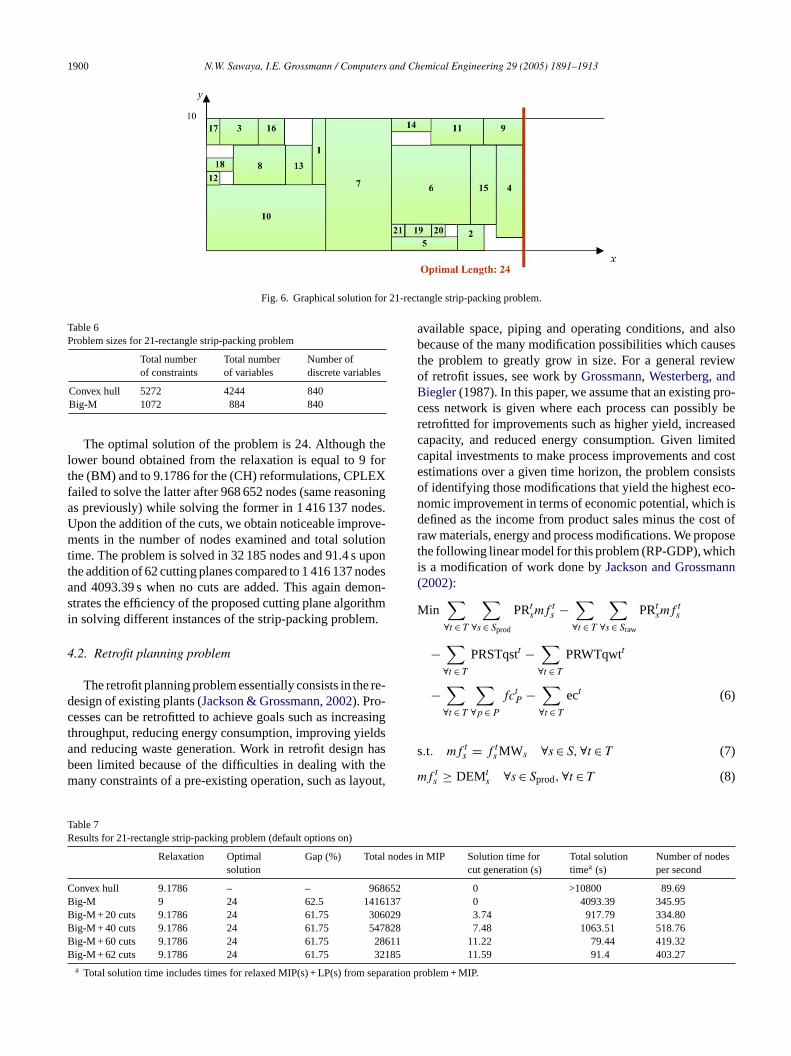
Fig. 6. Graphical solution for 21-rectangle strip-packing problem.
Table 6Problem sizes for 21-rectangle strip-packing problem
Total numberof constraints
Total numberof variables
Number ofdiscrete variables
Convex hull 5272 4244 840Big-M 1072 884 840
The optimal solution of the problem is 24. Although thelower bound obtained from the relaxation is equal to 9 forthe (BM) and to 9.1786 for the (CH) reformulations, CPLEXfailed to solve the latter after 968 652 nodes (same reasoningas previously) while solving the former in 1 416 137 nodes.Upon the addition of the cuts, we obtain noticeable improve-ments in the number of nodes examined and total solutiontime. The problem is solved in 32 185 nodes and 91.4 s uponthe addition of 62 cutting planes compared to 1 416 137 nodesand 4093.39 s when no cuts are added. This again demon-strates the efficiency of the proposed cutting plane algorithmin solving different instances of the strip-packing problem.
4.2. Retrofit planning problem
The retrofit planning problem essentially consists in the re-design of existing plants (Jackson & Grossmann, 2002). Pro-cesses can be retrofitted to achieve goals such as increasingthroughput, reducing energy consumption, improving yieldsand reducing waste generation. Work in retrofit design hasbeen limited because of the difficulties in dealing with themany constraints of a pre-existing operation, such as layout,
available space, piping and operating conditions, and alsobecause of the many modification possibilities which causesthe problem to greatly grow in size. For a general reviewof retrofit issues, see work byGrossmann, Westerberg, andBiegler(1987). In this paper, we assume that an existing pro-cess network is given where each process can possibly beretrofitted for improvements such as higher yield, increasedcapacity, and reduced energy consumption. Given limitedcapital investments to make process improvements and costestimations over a given time horizon, the problem consistsof identifying those modifications that yield the highest eco-nomic improvement in terms of economic potential, which isdefined as the income from product sales minus the cost ofraw materials, energy and process modifications. We proposethe following linear model for this problem (RP-GDP), whichis a modification of work done byJackson and Grossmann(2002):
Min∑∀t ∈ T
∑∀s ∈ Sprod
PRtsmf t
s −∑∀t ∈ T
∑∀s ∈ Sraw
PRtsmf t
s
−∑∀t ∈ T
PRSTqstt −∑∀t ∈ T
PRWTqwtt
−∑∀t ∈ T
∑∀p ∈ P
fctP −
∑∀t ∈ T
ect (6)
s
m
Table 7Results for 21-rectangle strip-packing problem (default options on)
l nodes
C 652B 137B 6029B 7828B 8611B 2185
eparat
Relaxation Optimalsolution
Gap (%) Tota
onvex hull 9.1786 – – 968ig-M 9 24 62.5 1416ig-M + 20 cuts 9.1786 24 61.75 30ig-M + 40 cuts 9.1786 24 61.75 54ig-M + 60 cuts 9.1786 24 61.75 2ig-M + 62 cuts 9.1786 24 61.75 3a Total solution time includes times for relaxed MIP(s) + LP(s) from s
.t. mf ts = f t
s MWs ∀s ∈ S, ∀t ∈ T (7)
f ts ≥ DEMt
s ∀s ∈ Sprod, ∀t ∈ T (8)
in MIP Solution time forcut generation (s)
Total solutiontimea (s)
Number of nodesper second
0 >10800 89.690 4093.39 345.953.74 917.79 334.807.48 1063.51 518.76
11.22 79.44 419.3211.59 91.4 403.27
ion problem + MIP.

N.W. Sawaya, I.E. Grossmann / Computers and Chemical Engineering 29 (2005) 1891–1913 1901
mf ts ≤ SUPt
s ∀s ∈ Sraw, ∀t ∈ T (9)∑∀s ∈ Snin
mf ts =
∑∀s ∈ Snout
mf ts ∀n ∈ N, ∀t ∈ T (10)
∑∀s ∈ Spin
mf ts =
∑∀s ∈ Spout
mf ts + unrcttp ∀p ∈ P, ∀t ∈ T (11)
∨∀m ∈ M
Ytpm
f ts = f t
plmt
(GMAt
s
GMAplmt
)ETAt
pm∑∀s ∈ Spin
mf ts ≤ CAPt
pm
∀s ∈ Spout, ∀p ∈ P, ∀t ∈ T (12)
∨∀m ∈ M
[Wt
pm
fctp = FCt
pm
]∀p ∈ P, ∀t ∈ T (13)
qtsk = mf t
s CPs(Ttsoutk
− T tsink
) ∀s ∈ Scold, ∀k ∈ K, ∀t ∈ T
(14)
Ytpm → ∧
τ>tYτ
pm ∀p ∈ P, ∀t ∈ T, ∀m ∈ M\m1 (19)
Wtpm → ∧
τ =tWt
p1 ∀p ∈ P, ∀t ∈ T, ∀m ∈ M\m1 (20)
Ytp1 → Wt
p1 ∀p ∈ P, ∀t ∈ T (21)
Ytpm ∧
τ<t¬Yτ
pm → Wtpm ∀p ∈ P, ∀t ∈ T, ∀m ∈ M\m1 (22)
Xtj → ∧
τ>tXτ
j ∀t ∈ T, ∀j ∈ J\j1 (23)
V tj → ∧
τ =tV t
1 ∀t ∈ T, ∀j ∈ J\j1 (24)
Xt1 → V t
1 ∀t ∈ T (25)
Xtj ∧
τ<t¬Xτ
j → V tj ∀t ∈ T, ∀j ∈ J\j1 (26)
mf ts , f
ts ∈R1
+ ∀s ∈ S, ∀t ∈ T
f tlmt,p, unrcttp, fct
p ∈R1+ ∀p ∈ P, ∀t ∈ T
qtsk ∈R1
+ ∀s ∈ S, ∀k ∈ K, ∀t ∈ T
qstt , qwtt , ect ∈R1+ ∀t ∈ T
t t t 1
,ts
olar
by
-ero
flow
-
are
s
qtsk = mf t
s CPs(Ttsink
− T tsoutk
) ∀s ∈ Shot, ∀k ∈ K, ∀t ∈ T
(15)
Xt1
qstt =∑
∀k ∈ K
∑∀s ∈ Scold
qtsk
qwtt =∑
∀k ∈ K
∑∀s ∈ Shot
qtsk
∨
Xt2
rtk − rt
k−1 − qsttk + qwttk =∑
∀s ∈ Shot
qtsk −
∑∀s ∈ Scold
qtsk
qstt =∑
∀k ∈ K
qsttk
qwtt = rt|K| +
∑∀k ∈ K
qwttk
∀k ∈ K, ∀t ∈ T (16)
[V t
1
ect = EFCt1
]∨
[V t
2
ect = EFCt2
]∀t ∈ T (17)
∑∀p ∈ P
fctp + ect +
∑∀s ∈ Sraw
PRtsmf t
s + PRSTqstt
+ PRWTqwtt ≤ INV t ∀t ∈ T (18)
qstk, qwtk, rk ∈R+ ∀k ∈ K, ∀t ∈ T
Ytpm, Wt
pm ∈ True, False ∀p ∈ P, ∀t ∈ T, ∀m ∈ M
Xtj, V
tj ∈ True, False ∀j ∈ J, ∀t ∈ T
The objective function(6) includes revenues from salescosts of raw material, utility costs, as well as capital cosfct
p and energy costs ect over time periodst∈T. Equation(7)represents an equivalence relation between mass and mflow rates, equations(8) and(9) ensure that mass flow ratesfor products and raw materials are respectively boundeddemand and supply parameters, and equations(10) and(11)serve as mass balances around nodesn∈N and processesp∈P,respectively. The first set of disjunctions(12) selects one ofthe operating modes for the retrofit projectm∈M, for ev-ery processp∈P, in every time periodt∈T, where projectsm include modifying either nothing at all (m1∈M), processconversion (m2∈M), capacity (m3∈M) or both (m4∈M). Thesecond set of disjunctions(13)enforces the cost of the aforementioned modifications, where capital costs are set to z(fct
p = 0) if nothing is modified. Equations(14) and (15)serve as equivalence relations between energy and massrate variables, while disjunction(s)(16) select the appropri-ate operating modeXt
j ∀j ∈ J so thatXt1 corresponds to no
energy integration andXt2 enforces the transshipment equa
tions (Biegler, Grossmann, & Westerberg, 1997). ThroughBoolean variablesV t
j , the set of disjunctions(17)enforce thecost associated with energy reduction, where these costsset to zero (ect = 0) if nothing is modified (V t
1 = True). Equa-tion(18)limits the expenses for the retrofit project. Equation

1902 N.W. Sawaya, I.E. Grossmann / Computers and Chemical Engineering 29 (2005) 1891–1913
(21) and(22), (25) and(26) are logical conditions that con-nect, respectively, disjunctions(12) to (13) and disjunctions(16) to (17) with each other, and equations(19) and (20),(23) and (24) impose logical conditions between disjunctsin every set of corresponding disjunctions. Essentially, theselogical equations constrain the problem such that costs asso-ciated with conversion and/or capacity are enforced exactlyonce for every processp∈P in every time periodt∈T, andsuch that costs associated with energy reduction are enforcedexactly once per time periodt∈T.
We consider inFig. 7a 10 process instance of the retrofitplanning problem (RP-GDP) that involves the production ofproducts (G, H, I, J, K, L, M) from raw materials (A, B, C,D, E).
We use a 1-year planning horizon of four time periods eachconsisting of 3 months. Modifications for increased conver-sion and capacity only are considered, and black-box (in-put/output) models are used for each process. We do not in-clude explicit data for this problem because of its size. Theproblem was transformed into an MIP model by using boththe big-M and convex hull reformulations given inAppendixC. Problem sizes for both reformulations are listed inTable 8,while the graphical solution to this problem is presented inFig. 8.
We solved this problem using the proposed cutting planealgorithm, and compared the resulting solutions to those from
Table 8Problem sizes for 10-process retrofit planning problem
Total numberof constraints
Total numberof variables
Number ofdiscrete variables
Convex hull 2505 1417 320Big-M 1957 697 320
the convex hull and big-M reformulations inTables 9 and 10.We first examine the results with all MIP algorithmic optionsturned off (seeTable 9).
The optimal solution of the problem is US$ 7 868 786.32.The upper bound obtained from the relaxation is equal toUS$ 11 743 915.93 for the (BM) reformulation and US$7 868 786.32 for the (CH) reformulation, and the problemwas solved in 1 607 486 nodes using the (BM) reformula-tion, as opposed to the (CH) reformulation, which requiredonly 2155 nodes. Clearly, the (CH) feasible region is tighterthan that of the big-M, which results in large savings in com-putational time (5.8 s versus 1913.67 s). After the addition of40 cutting planes to the (BM) reformulation, we are able toreduce the relaxation gap by nearly 40% and solve the prob-lem in 656.15 s while examining 403 463 nodes in the B&Btree. Upon the successive addition of more cuts, the numberof nodes examined is further reduced, which results in a fur-ther decrease in total solution time. Finally, 196 cuts were
Fig. 7. Ten process retrofit pla
nning problem flowsheet.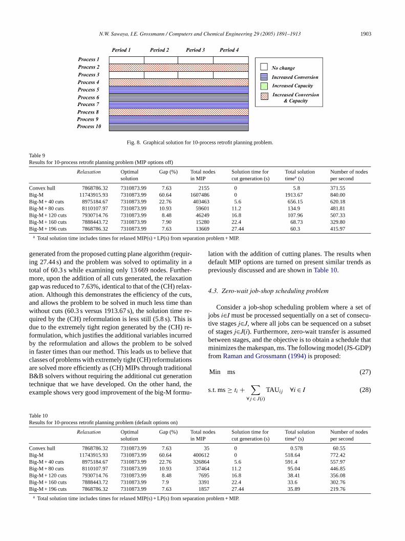
N.W. Sawaya, I.E. Grossmann / Computers and Chemical Engineering 29 (2005) 1891–1913 1903
Fig. 8. Graphical solution for 10-process retrofit planning problem.
Table 9Results for 10-process retrofit planning problem (MIP options off)
Relaxation Optimalsolution
Gap (%) Total nodesin MIP
Solution time forcut generation (s)
Total solutiontimea (s)
Number of nodesper second
Convex hull 7868786.32 7310873.99 7.63 2155 0 5.8 371.55Big-M 11743915.93 7310873.99 60.64 1607486 0 1913.67 840.00Big-M + 40 cuts 8975184.67 7310873.99 22.76 403463 5.6 656.15 620.18Big-M + 80 cuts 8110107.97 7310873.99 10.93 59601 11.2 134.9 481.81Big-M + 120 cuts 7930714.76 7310873.99 8.48 46249 16.8 107.96 507.33Big-M + 160 cuts 7888443.72 7310873.99 7.90 15280 22.4 68.73 329.80Big-M + 196 cuts 7868786.32 7310873.99 7.63 13669 27.44 60.3 415.97
a Total solution time includes times for relaxed MIP(s) + LP(s) from separation problem + MIP.
generated from the proposed cutting plane algorithm (requir-ing 27.44 s) and the problem was solved to optimality in atotal of 60.3 s while examining only 13 669 nodes. Further-more, upon the addition of all cuts generated, the relaxationgap was reduced to 7.63%, identical to that of the (CH) relax-ation. Although this demonstrates the efficiency of the cuts,and allows the problem to be solved in much less time thanwithout cuts (60.3 s versus 1913.67 s), the solution time re-quired by the (CH) reformulation is less still (5.8 s). This isdue to the extremely tight region generated by the (CH) re-formulation, which justifies the additional variables incurredby the reformulation and allows the problem to be solvedin faster times than our method. This leads us to believe thatclasses of problems with extremely tight (CH) reformulationsare solved more efficiently as (CH) MIPs through traditionalB&B solvers without requiring the additional cut generationtechnique that we have developed. On the other hand, theexample shows very good improvement of the big-M formu-
lation with the addition of cutting planes. The results whendefault MIP options are turned on present similar trends aspreviously discussed and are shown inTable 10.
4.3. Zero-wait job-shop scheduling problem
Consider a job-shop scheduling problem where a set ofjobsi∈I must be processed sequentially on a set of consecu-tive stagesj∈J, where all jobs can be sequenced on a subsetof stagesj∈J(i). Furthermore, zero-wait transfer is assumedbetween stages, and the objective is to obtain a schedule thatminimizes the makespan, ms. The following model (JS-GDP)from Raman and Grossmann (1994)is proposed:
Min ms (27)
s.t. ms≥ ti +∑
∀j ∈ J(i)
TAUij ∀i ∈ I (28)
Table 10Results for 10-process retrofit planning problem (default options on)
Relaxation Optimalsolution
Gap (%) Total nodesin MIP
Solution time forcut generation (s)
Total solutiontimea (s)
Number of nodesper second
Convex hull 7868786.32 7310873.99 7.63 35 0 0.578 60.55Big-M 11743915.93 7310873.99 60.64 400612 0 518.64 772.42B 32686B 3746B 7695B 3391B 1857
eparat
ig-M + 40 cuts 8975184.67 7310873.99 22.76ig-M + 80 cuts 8110107.97 7310873.99 10.93ig-M + 120 cuts 7930714.76 7310873.99 8.48ig-M + 160 cuts 7888443.72 7310873.99 7.9ig-M + 196 cuts 7868786.32 7310873.99 7.63a Total solution time includes times for relaxed MIP(s) + LP(s) from s
4 5.6 591.4 557.974 11.2 95.04 446.85
16.8 38.41 356.0822.4 33.6 302.7627.44 35.89 219.76
ion problem + MIP.
1904 N.W. Sawaya, I.E. Grossmann / Computers and Chemical Engineering 29 (2005) 1891–1913
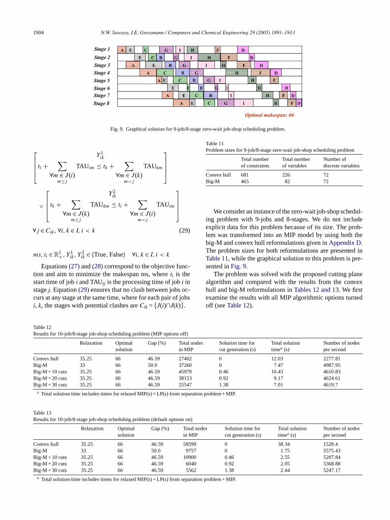
Fig. 9. Graphical solution for 9-job/8-stage zero-wait job-shop scheduling problem.
Y1ik
ti +∑
∀m ∈ J(i)m≤j
TAUim ≤ tk +∑
∀m ∈ J(k)m<j
TAUkm
∨
Y2ik
tk +∑
∀m ∈ J(k)m≤j
TAUkm ≤ ti +∑
∀m ∈ J(i)m<j
TAUim
∀j ∈ Cik, ∀i, k ∈ I, i < k (29)
ms, ti ∈R1+, Y1
ik, Y2ik ∈ True, False ∀i, k ∈ I, i < k
Equations(27)and(28)correspond to the objective func-tion and aim to minimize the makespan ms, whereti is thestart time of jobi and TAUij is the processing time of jobi instagej. Equation(29)ensures that no clash between jobs oc-curs at any stage at the same time, where for each pair of jobsi, k, the stages with potential clashes areCik =J(i)∩J(k).
Table 11Problem sizes for 9-job/8-stage zero-wait job-shop scheduling problem
Total numberof constraints
Total numberof variables
Number ofdiscrete variables
Convex hull 681 226 72Big-M 465 82 72
We consider an instance of the zero-wait job-shop schedul-ing problem with 9-jobs and 8-stages. We do not includeexplicit data for this problem because of its size. The prob-lem was transformed into an MIP model by using both thebig-M and convex hull reformulations given inAppendix D.The problem sizes for both reformulations are presented inTable 11, while the graphical solution to this problem is pre-sented inFig. 9.
The problem was solved with the proposed cutting planealgorithm and compared with the results from the convexhull and big-M reformulations inTables 12 and 13. We firstexamine the results with all MIP algorithmic options turnedoff (seeTable 12).
Table 12Results for 10-job/8-stage job-shop scheduling problem (MIP options off)
l nodes Solution time forcut generation (s)
Total solutiontimea (s)
Number of nodesper second
C 2 0 12.03 2277.81B 0 0 7.47 4987.95B 0 0.46 10.43 4610.83B 3 0.92 9.17 4624.61B 7 1.38 7.01 4619.7
eparation problem + MIP.
TR ns on)
tal nodeIP
C 99B 57B 00B 40B 62
eparat
Relaxation Optimalsolution
Gap (%) Totain MIP
onvex hull 35.25 66 46.59 2740ig-M 33 66 50.0 3726ig-M + 10 cuts 35.25 66 46.59 4597ig-M + 20 cuts 35.25 66 46.59 3815ig-M + 30 cuts 35.25 66 46.59 2554a Total solution time includes times for relaxed MIP(s) + LP(s) from s
able 13esults for 10-job/8-stage job-shop scheduling problem (default optio
Relaxation Optimalsolution
Gap (%) Toin M
onvex hull 35.25 66 46.59 585ig-M 33 66 50.0 97ig-M + 10 cuts 35.25 66 46.59 109ig-M + 20 cuts 35.25 66 46.59 60ig-M + 30 cuts 35.25 66 46.59 55a Total solution time includes times for relaxed MIP(s) + LP(s) from s
s Solution time forcut generation (s)
Total solutiontimea (s)
Number of nodesper second
0 38.34 1528.40 1.75 5575.430.46 2.55 5207.840.92 2.05 5368.881.38 2.44 5247.17
ion problem + MIP.

N.W. Sawaya, I.E. Grossmann / Computers and Chemical Engineering 29 (2005) 1891–1913 1905
The optimal solution of the problem is 66. The lowerbound obtained from the relaxation is equal to 33 for the(BM) reformulation and 35.25 for the (CH) reformulation,and the problem was solved in 37 260 nodes using the (BM)reformulation, as opposed to the (CH) reformulation, whichrequired 27 402 nodes. It is clear that the (CH) feasible re-gion is not much tighter than that of the (BM) as seen fromthe poor relaxation value and the number of nodes exam-ined in the B&B tree. This causes the solution time of (CH)to be larger than that of (BM) due to the greater number ofvariables and constraints in the formulation (12.03 s versus7.47 s). Furthermore, one can conjecture that since the (CH)feasible region is not much tighter than that of the (BM), theeffect that the cuts will have on overall solution times andnumber of nodes examined will be minimal. In fact, afterthe addition of 30 cutting planes to the (BM) reformulation,we are able to solve the problem in 7.01 s while examining25 547 nodes in the B&B tree, only slight improvements onthe results obtained using the (BM) reformulation. This leadsus to believe that classes of problems with extremely loose(CH) reformulations are solved efficiently enough as (BM)MIPs through traditional B&B solvers. The proposed cut-ting plane algorithm does not improve solution times for thisclass of problems since the amount of time required to gen-erate the cuts does not justify the (loose) tightening the cutsprovide. The results when default MIP options are turned onp howni trip-p CH)r
5
d thata M re-f slyd king,r rob-l osedm lax-a h toj u-l rob-l , weh thodr trofitp heret oser
thatc thej in-fi ificp botht nt in
the literature and to extend the work to solution methods forconvex non-linear GDP problems.
Acknowledgement
The authors would like to gratefully acknowledge finan-cial support from the National Science Foundation underGrant ACI-0121497.
Appendix A. Proofs of propositions
Proof of Proposition 1.
(1) (FR-SEP)⊆(FR-BM): SeeGrossmann and Lee (2003),Proposition 4.
(2) (FRP-SEP) is convex: FromCeria and Soares (1999)andGrossmann and Lee (2003), we know that (FR-SEP) isa convex set. Thus, since (FRP-SEP) is the projectionof (FR-SEP) from the (z,v) space onto thez space, andprojection preserves convexity, then (FRP-SEP) is alsoconvex.
Proof of Proposition 2.
(1) Let φ : Rn → R be defined as||z − zbm||. Thenφ is a
-
s of1),
-
(anw
-
i
resent similar trends as previously discussed and are sn Table 13(note once again, as in the case of the sacking problem, the poor results obtained using the (eformulation).
. Conclusion
We have presented in this paper a cutting plane methodds cuts generated from a separation problem to a big-
ormulation of a linear GDP problem. We have rigorouerived the cuts, and applied the method to the strip-pacetrofit planning and zero-wait job-shop scheduling pems. The results demonstrate the efficiency of the prop
ethod for a class of problems where the convex hull retion is tighter than that of the big-M, but not tight enoug
ustify the additional variables required by the (CH) reformation. An example within that class is the strip-packing pem where excellent results were obtained. Furthermoreave also highlighted some of the drawbacks of the meegarding other classes of problems which include the relanning and zero-wait job-shop scheduling problems, w
he convex hull relaxation was either too tight or too loespectively.
We intend to examine in the future different methodsould improve the algorithm, specifically as pertaining toudicious selection of those Lagrange multipliers (for thenity norm) that generate the “best” cuts for our specroblem. We also intend to compare the proposed cuts,
heoretically and computationally, to those already prese
convex function for the 1, 2 and∞ norms over all itsdomain. Also, fromProposition 1, we know that (FRPSEP) is a convex set. Furthermore, let (zsep, vsep) be theoptimal solution of (SEP). Clearly, from the propertieprojection,zsepwould be the optimal solution of (SEPwhere (SEP1) is as follows:
Min φ(z) = ||z − zbm||s.t. z ∈ (FRP-SEP)
From Theorem 3.4.3 inBazarra and Shetty (1979), ifzsep is an optimal solution to (SEP1), thenφ has a subgradientξ at zsepsuch thatξT(z − zsep) ≥ 0 ∀ z∈(FRP-SEP).
2) FromProposition 1, we know that (FR-SEP)⊆(FR-BM).In the case wherezbm∈(FRP-SEP), obviously no cut cbe generated. Otherwise,zbm/∈(FRP-SEP) and we shothat the above inequality cuts offzbm. From (1) we knowthat ξT(z − zsep) ≥ 0 ∀ z ∈ (FRP-SEP). Furthermore,ξis a subgradient ofφ(z) at zsep. By definition of subgradient (Nemhauser & Wolsey, 1999), for convexφ(z), wehave:
φ(z) − φ(zsep) ≥ ξT(z − zsep) ∀z ∈ (FR-SEP)
⇔ ∥∥z − zbm∥∥ − ∥∥zsep− zbm
∥∥ ≥ ξT(z − zsep)
∀z ∈ (FR-SEP)
f z ≡ zbm, then
||zbm − zbm|| − ||zsep− zbm|| ≥ ξT(zbm − zsep)
⇔ ξT(zbm − zsep) ≤ −||zsep− zbm|| < 0

1906 N.W. Sawaya, I.E. Grossmann / Computers and Chemical Engineering 29 (2005) 1891–1913
Thus,zbm does not satisfyξT(z − zsep) ≥ 0 and is thereforecut off by the inequality.
Proof of Proposition 3. If φ is differentiable overS, thenφ isdifferentiable atzsep. It follows from Lemma 3.3.2 inBazarraand Shetty (1979)that the only element of the subdifferentialof φ is φ(zsep).
Proof of Proposition 4. If φ is defined asφ(z) = ||z −zbm||22, thenφ is differentiable and fromProposition 3, thecollection of subgradients ofφ at zsep is the singleton setφ(zsep). Thus,
φ(zsep) = (zsep− zbm)T(zsep− zbm) and
∇φ(zsep) = 2(zsep− zbm)
Proof of Proposition 5. Let φ : S → R be defined asφ(z) = ||z − zbm||∞ in (SEP). Then (SEP) can be rewrittenas:
Min u
s.t. u ≥ zi − zbmi ∀i ∈ M
u ≥ zbmi − zi ∀i ∈ M
(FR-SEP)
(A.1)
From Proposition 1, we know that (FR-SEP) is convex.F hus,(mn
v ntsfR
l
L
aa
0 ⇒i
|(u =
Now let us define the following matrixH with columnshi
asH ≡ [I| − I] and the following vectorµ asµ ≡[
µ+µ−
].
We claim that ifξ = Hµ, then the existence of a vector
µsep≡[
µsep+
µsep−
]≡
[µi+µi−
]∀i ∈ Msepin (A.3) is equivalent
to the existence of a vectorξsepin the set:
∂sepφ ≡ ξsep|ξsep∈ convi ∈ Nsep
hi (A.4)
such that
ξ + R1Tρsep= 0
R2Tρsep= 0
ρsep≥ 0
where(A.4) is the subdifferential ofφ, ξsepis a subgradient ofφ(zsep) andNsep≡ i : |zi − zbm
i | is maximized, accordingto Section 14.1 and Lemma 14.2.2 inFletcher (1987).
In essence, we are claiming that in order to obtain a subgra-dient vectorξsepof φ(zsep) in (A.4), one needs only to obtaina set of Lagrange multipliersµsepfrom (A.3) (thus, the exis-tence of one is equivalent to the existence of the other). Weprove the claim as follows.
∂
s
ξ
R
ρ
⇔
s
ξ
R
urthermore, all the constraints in (FR-SEP) are linear. TFR-SEP) corresponds to a polytope in the (z, ν) space, and∃atricesR1,R2 with dimensionsm × (n × ∑
k ∈ K |Jk|), m ×, respectively, and vectorr ∈Rm such that (FR-SEP)≡ (z,)|R1z + R2ν ≤ r. Note that the non-negativity constraior z andv are taken into account in the construction ofR1,2.
We can thus write(A.1) as:
Min u
s.t. u ≥ zi − zbmi ∀i ∈ M
u ≥ zbmi − zi ∀i ∈ M
R1z + R2ν ≤ r
(A.2)
The appropriate Lagrangean function of(A.2) is as fol-ows:
= u +∑i ∈ M
µi+(zi − zbmi − u) +
∑i ∈ M
µi−(zbmi − zi − u)
+ ρT(R1z + R2ν − r)
nd it is implied at (zsep, νsep, usep) that multipliersµsep+ , µ
sep− ,
ndρsepexist such that:
∂L
∂u(zsep, νsep, usep) = 0 ⇒ 1 −
∑i ∈ Msep
µi+ −∑
i ∈ Msep
µi− =
∇zL(zsep, νsep, usep) = 0 ⇒ [µ+ − µ−] + R1Tρsep= 0
∇νL(zsep, νsep, usep) = 0 ⇒ R2Tρsep= 0
µ+i , µ−
i , ρsep≥ 0 ∀i ∈ Msep, whereMsep≡ activeM ≡ i
∑∈ Msep
(µi+ + µi−) = 1
zi − zbmi ) ∨ (u = zbm
i − zi)∀i ∈ M
(A.3)
From(A.4), we have,sepφ ≡ ξsep|ξsep∈ conv
i ∈ Nsephi
uch that
+ R1Tρsep= 0
2Tρsep= 0
sep≥ 0
ξsep=∑
i ∈ Nsep
αihi with∑
i ∈ Nsep
αi = 1,
αi ≥ 0 from the convex hull definition
uch that
+ R1Tρsep= 0
2Tρsep= 0

N.W. Sawaya, I.E. Grossmann / Computers and Chemical Engineering 29 (2005) 1891–1913 1907
ρsep ≥ 0
⇔ ξsep= Hsepαsep= [Isep| − Isep]
[α
sep+
αsep−
]
= [αsep+ − α
sep− ]
such that∑i ∈ Nsep
αi+ + αi− = 1, αsep≥ 0
ξ + R1Tρsep= 0
R2Tρsep= 0
ρsep≥ 0
(A.5)
If ξ = Hµ ⇔ ξ = [I| − I]
[µ+µ−
]= [µ+ − µ−]
then
ξsep= [µsep+ − µ
sep− ] and ξi = [µi+ − µi−] ∀i ∈ Nsep
but from (A.5) we know thatξsep= [αsep+ − α
sep− ],so α =µ
and(A.5) becomes:
ξsep= [µsep+ − µ
sep− ]
∑
a[
Ap
B
xj + Lj ≤ xi + BIGM2ij(1 − w2
ij) ∀i, j ∈ N, i < j
yi − Hi ≥ yj − BIGM3ij(1 − w3
ij) ∀i, j ∈ N, i < j
yj − Hj ≥ yi − BIGM4ij(1 − w4
ij) ∀i, j ∈ N, i < j∑d ∈ D
wdij = 1 ∀i, j ∈ N, i < j
xi ≤ UBi − Li ∀i ∈ N
Hi ≤ yi ≤ W ∀i ∈ N
lt, xi, yi ∈R1+, wdij ∈ 0, 1 ∀d ∈ D, ∀i, j ∈ N, i < j
whereD =1, 2, 3, 4.
B.2. Convex hull reformulation of (SP-GDP)
Min lt
s.t. lt ≥ xi + Li ∀i ∈ N
xk =∑d ∈ D
νdkij ∀i, j, k ∈ N, i < j, k = i ∨ j
yk =∑d ∈ D
ωdkij ∀i, j, k ∈ N, i < j, k = i ∨ j
ν1iij − ν1
jij ≤ −Liw1ij ∀i, j ∈ N, i < j
s.t.i ∈ Nsep
µi+ + µi− = 1, µi ≥ 0
[µ+ − µ−] + R1Tρsep= 0
R2Tρsep= 0
ρsep≥ 0
(A.6)
Clearly, Nsep≡ Msep and we have thus recovered(A.3)nd shown that the form of the subgradient is indeedξsep=µ
sep+ − µ
sep− ].
ppendix B. Reformulations of strip-packingroblem (SP-GDP)
.1. Big-M reformulation of (SP-GDP)
Min lt
s.t. lt ≥ xi + Li ∀i ∈ N
xi + Li ≤ xj + BIGM1ij(1 − w1
ij) ∀i, j ∈ N, i < j
ν2jij − ν2
iij ≤ −Ljw2ij ∀i, j ∈ N, i < j
ω3iij − ω3
jij ≥ Hiw3ij ∀i, j ∈ N, i < j
ω4jij − ω4
iij ≥ Hjw4ij ∀i, j ∈ N, i < j∑
d ∈ D
wdij = 1 ∀i, j ∈ N, i < j
νdkij ≤ UBd
kijwdij ∀d ∈ D, ∀i, j, k ∈ N, i < j, k = i ∨ j
ωdkij ≤ UBd
kijwdij ∀d ∈ D, ∀i, j, k ∈ N, i < j, k = i ∨ j
xi ≤ UBi − Li ∀i ∈ N
Hi ≤ yi ≤ W ∀i ∈ N
lt, xi, yi, νdkij, ω
dkij
∈R1+, wdij ∈ 0, 1 ∀d ∈ D, ∀i, j, k ∈ N, i < j, k = i ∨ j
whereD =1, 2, 3, 4.

1908 N.W. Sawaya, I.E. Grossmann / Computers and Chemical Engineering 29 (2005) 1891–1913
Appendix C. Reformulations of retrofit planning problem (RP-GDP)
C.1. Big-M reformulation of (RP-GDP)
Min Z =∑t ∈ T
∑s ∈ Sprod
PRtsmf t
s −∑t ∈ T
∑s ∈ Sraw
PRstmf t
s −∑t ∈ T
PRSTqstt
−∑t ∈ T
PRWTqwtt −∑t ∈ T
∑m ∈ M
∑p ∈ P
FCtpmwt
pm −∑t ∈ T
∑j ∈ J
EFCtj
s.t. mf ts = f t
s MWs ∀s ∈ S, ∀t ∈ T
mf ts ≥ DEMt
s ∀s ∈ Sprod, ∀t ∈ T
mf ts ≤ SUPt
s ∀s ∈ Sraw, ∀t ∈ T∑s ∈ Snin
mf ts =
∑s ∈ Snout
mf ts ∀n ∈ N, ∀t ∈ T
∑s ∈ Spin
mf ts =
∑s ∈ Spout
mf ts + unrcttp ∀p ∈ P, ∀t ∈ T
f ts ≤ f t
plmt
(GMAt
s
GMAplmt
)ETAt
pm + BIGMtpm(1 − yt
pm) ∀s ∈ Spout, ∀p ∈ P, ∀m ∈ M, ∀t ∈ T
f ts ≥ f t
plmt
(GMAt
s
GMAplmt
)ETAt
pm − BIGMtpm(1 − yt
pm) ∀s ∈ Spout, ∀p ∈ P, ∀m ∈ M, ∀t ∈ T
∑mf t
s ≤ CAPtpm + BIGMt
pm(1 − ytpm) ∀p ∈ P, ∀m ∈ M, ∀t ∈ T
s ∈ Spin
fctp ≤ FCt
pm + BIGMtpm(1 − wt
pm) ∀p ∈ P, ∀m ∈ M, ∀t ∈ T
fctp ≥ FCt
pm − BIGMtpm(1 − wt
pm) ∀p ∈ P, ∀m ∈ M, ∀t ∈ T
qtsk = mf t
s CPs(T tsoutk
− T tsink
) ∀s ∈ Scold, ∀k ∈ K, ∀t ∈ T
qtsk = mf t
s CPs(T tsink
− T tsoutk
) ∀s ∈ Shot, ∀k ∈ K, ∀t ∈ T
qstt ≤∑k ∈ K
∑s ∈ Scold
qtsk + BIGMt
1,1(1 − xt1) ∀t ∈ T
qstt ≥∑k ∈ K
∑s ∈ Scold
qtsk − BIGMt
1,1(1 − xt1) ∀t ∈ T
qwtt ≤∑k ∈ K
∑s ∈ Shot
qtsk + BIGMt
2,1(1 − xt1) ∀t ∈ T
qwtt ≥∑k ∈ K
∑s ∈ Shot
qtsk − BIGMt
2,1(1 − xt1) ∀t ∈ T
rtk − rt
k−1 − qsttk + qwttk ≤∑
s ∈ Shot
qtsk −
∑s ∈ Scold
qtsk + BIGMt
1,2(1 − xt2) ∀k ∈ K, ∀t ∈ T
rtk − rt
k−1 − qsttk + qwttk ≥∑
s ∈ Shot
qtsk −
∑s ∈ Scold
qtsk − BIGMt
1,2(1 − xt2) ∀k ∈ K, ∀t ∈ T

N.W. Sawaya, I.E. Grossmann / Computers and Chemical Engineering 29 (2005) 1891–1913 1909
qstt ≤∑k ∈ K
qsttk + BIGMt2,2(1 − xt
2) ∀t ∈ T
qstt ≥∑k ∈ K
qsttk − BIGMt2,2(1 − xt
2) ∀t ∈ T
qwtt ≤ rt|K| +
∑k ∈ K
qwttk + BIGMt3,2(1 − xt
2) ∀t ∈ T
qwtt ≥ r|K|t +∑k ∈ K
qwttk − BIGMt2,2(1 − xt
2) ∀t ∈ T
ect ≤ EFCtj + BIGMt
j(1 − vtj) ∀j ∈ J, ∀t ∈ T
ect ≥ EFCtj − BIGMt
j(1 − vtj) ∀j ∈ J, ∀t ∈ T∑
p ∈ P
fctp + ect +
∑s ∈ Sraw
PRts mfts + PRST qstt + PRWT qwtt ≤ INV t ∀t ∈ T
∑m ∈ M
ytpm = 1 ∀p ∈ P, ∀t ∈ T
∑m ∈ M
wtpm = 1 ∀p ∈ P, ∀t ∈ T
∑j ∈ J
xtj = 1 ∀t ∈ T
∑j ∈ J
vtj = 1 ∀t ∈ T
ytpm ≤ yτ
pm ∀p ∈ P, ∀t < τ ∈ T, ∀m ∈ M\m1
wtpm ≤ wτ
p1 ∀p ∈ P, ∀t = τ ∈ T, ∀m ∈ M\m1
ytp1 ≤ wt
p1 ∀p ∈ P, ∀t ∈ T
ytpm ≤ wt
pm +|T |−1∑τ=1
yt−τpm ∀p ∈ P, ∀t ∈ T, ∀m ∈ M\m1
xt2 ≤ xτ
1 ∀t < τ ∈ T
vt2 ≤ vτ
1 ∀t = τ ∈ T
xt1 ≤ vt
1 ∀t ∈ T
xt2 ≤ vt
2 +|T |−1∑τ=1
xt−τ2 ∀t ∈ T
mf ts , f
ts ∈R1+ ∀s ∈ S, ∀t ∈ T
f tplmt
, unrcttp, fctp ∈R1+ ∀p ∈ P, ∀t ∈ T
qskt ∈R1+ ∀s ∈ S, ∀k ∈ K, ∀t ∈ T
qstt , qwtt , ect ∈R1+ ∀t ∈ T
qsttk, qwttk, rtk ∈R1+ ∀k ∈ K, ∀t ∈ T
ytpm, wt
pm ∈ 0, 1 ∀p ∈ P, ∀t ∈ T, ∀m ∈ M
xtj, v
tj ∈ 0, 1 ∀j ∈ J, ∀t ∈ T
1910 N.W. Sawaya, I.E. Grossmann / Computers and Chemical Engineering 29 (2005) 1891–1913
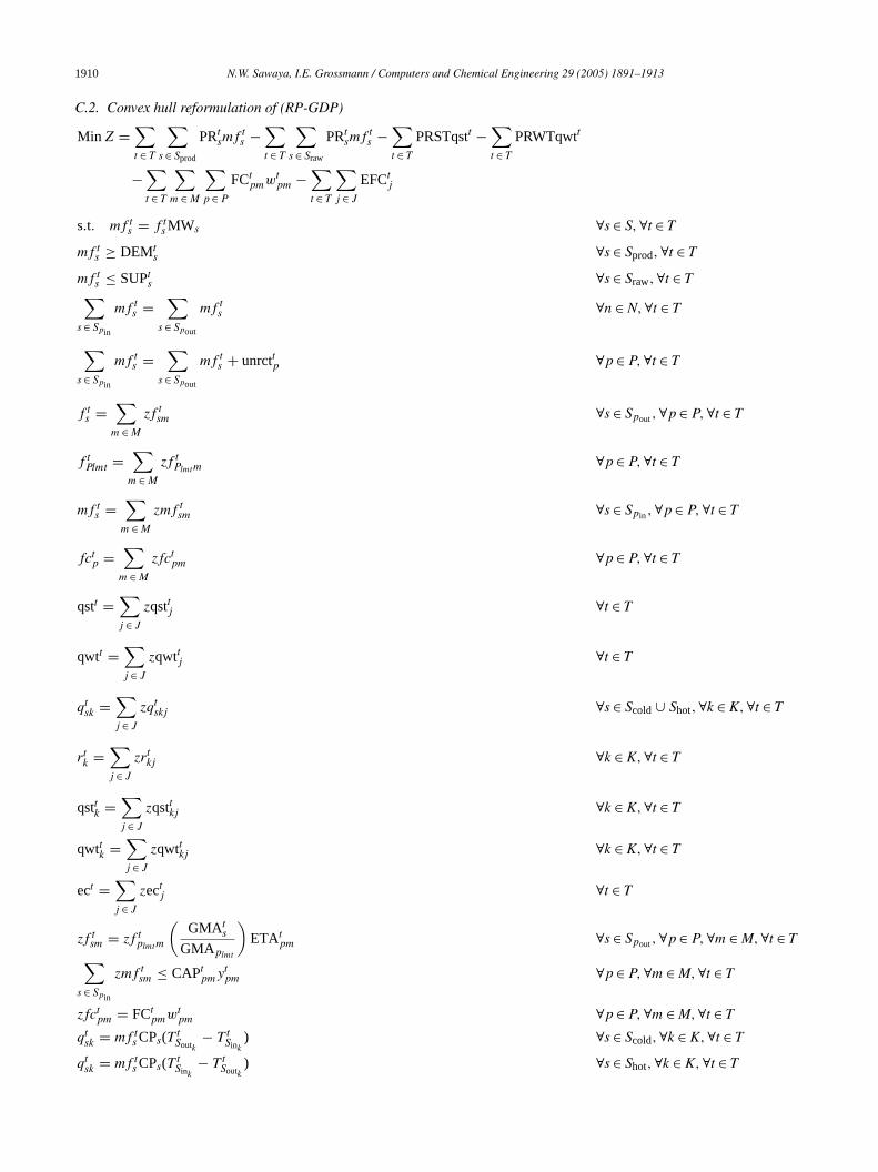
C.2. Convex hull reformulation of (RP-GDP)
Min Z =∑t ∈ T
∑s ∈ Sprod
PRtsmf t
s −∑t ∈ T
∑s ∈ Sraw
PRtsmf t
s −∑t ∈ T
PRSTqstt −∑t ∈ T
PRWTqwtt
−∑t ∈ T
∑m ∈ M
∑p ∈ P
FCtpmwt
pm −∑t ∈ T
∑j ∈ J
EFCtj
s.t. mf ts = f t
s MWs ∀s ∈ S, ∀t ∈ T
mf ts ≥ DEMt
s ∀s ∈ Sprod, ∀t ∈ T
mf ts ≤ SUPt
s ∀s ∈ Sraw, ∀t ∈ T∑s ∈ Spin
mf ts =
∑s ∈ Spout
mf ts ∀n ∈ N, ∀t ∈ T
∑s ∈ Spin
mf ts =
∑s ∈ Spout
mf ts + unrcttp ∀p ∈ P, ∀t ∈ T
f ts =
∑m ∈ M
zf tsm ∀s ∈ Spout, ∀p ∈ P, ∀t ∈ T
f tPlmt =
∑m ∈ M
zf tPlmtm
∀p ∈ P, ∀t ∈ T
mf ts =
∑m ∈ M
zmf tsm ∀s ∈ Spin , ∀p ∈ P, ∀t ∈ T
∑
fctp =m ∈ M
zfctpm ∀p ∈ P, ∀t ∈ T
qstt =∑j ∈ J
zqsttj ∀t ∈ T
qwtt =∑j ∈ J
zqwttj ∀t ∈ T
qtsk =
∑j ∈ J
zqtskj ∀s ∈ Scold ∪ Shot, ∀k ∈ K, ∀t ∈ T
rtk =
∑j ∈ J
zrtkj ∀k ∈ K, ∀t ∈ T
qsttk =∑j ∈ J
zqsttkj ∀k ∈ K, ∀t ∈ T
qwttk =∑j ∈ J
zqwttkj ∀k ∈ K, ∀t ∈ T
ect =∑j ∈ J
zectj ∀t ∈ T
zf tsm = zf t
plmtm
(GMAt
s
GMAplmt
)ETAt
pm ∀s ∈ Spout, ∀p ∈ P, ∀m ∈ M, ∀t ∈ T∑s ∈ Spin
zmf tsm ≤ CAPt
pmytpm ∀p ∈ P, ∀m ∈ M, ∀t ∈ T
zfctpm = FCt
pmwtpm ∀p ∈ P, ∀m ∈ M, ∀t ∈ T
qtsk = mf t
s CPs(T tSoutk
− T tSink
) ∀s ∈ Scold, ∀k ∈ K, ∀t ∈ T
qtsk = mf t
s CPs(T tSink
− T tSoutk
) ∀s ∈ Shot, ∀k ∈ K, ∀t ∈ T

N.W. Sawaya, I.E. Grossmann / Computers and Chemical Engineering 29 (2005) 1891–1913 1911
zqstt1 =∑k ∈ K
∑s ∈ Scold
zqtsk1 ∀t ∈ T
zqwtt1 =∑k ∈ K
∑s ∈ Shot
zqtsk1 ∀t ∈ T
zrtk2 − zrt
k−1,2 − zqsttk2 + zqwttk2 =∑
s ∈ Shot
zqtsk2 −
∑s ∈ Scold
zqtsk2 ∀k ∈ K, ∀t ∈ T
zqstt2 =∑k ∈ K
zqsttk2 ∀t ∈ T
zqwtt2 = zrt|K|2 +
∑k ∈ K
zqwttk2 ∀t ∈ T
zectj = EFCtjv
tj ∀j ∈ J, ∀t ∈ T∑
p ∈ P
fctp + ect +
∑s ∈ Sraw
PRtsmf t
s + PRSTqstt + PRWTqwtt ≤ INV t ∀t ∈ T
zf tsm ≤ BNDt
smytpm ∀s ∈ Spout, ∀p ∈ P, ∀m ∈ M, ∀t ∈ T
zf tPlmtm
≤ BNDtPlmtm
ytpm ∀p ∈ P, ∀m ∈ M, ∀t ∈ T
zmf tsm ≤ BNDt
smytpm ∀s ∈ Spin , ∀p ∈ P, ∀m ∈ M, ∀t ∈ T
zfctpm ≤ BNDt
pmwtpm ∀p ∈ P, ∀m ∈ M, ∀t ∈ T
zqstt ≤ BNDt xt ∀j ∈ J, ∀t ∈ T
j j jzqwttj ≤ BNDtjx
tj ∀j ∈ J, ∀t ∈ T, ∀t ∈ T
zqtskj ≤ BNDt
skjxtj ∀s ∈ Scold ∪ Shot, ∀k ∈ K, ∀j ∈ J, ∀t ∈ T
zrtkj ≤ BNDt
kjxtj ∀k ∈ K, ∀j ∈ J, ∀t ∈ T
zqsttkj ≤ BNDtkjx
tj ∀k ∈ K, ∀j ∈ J, ∀t ∈ T
zqwttkj ≤ BNDtkjx
tj ∀k ∈ K, ∀j ∈ J, ∀t ∈ T
zectj ≤ BNDtjv
tj ∀j ∈ J, ∀t ∈ T∑
m ∈ M
ytpm = 1 ∀p ∈ P, ∀t ∈ T
∑m ∈ M
wtpm = 1 ∀p ∈ P, ∀t ∈ T
∑j ∈ J
xtj = 1 ∀t ∈ T
∑j ∈ J
vtj = 1 ∀t ∈ T
ytpm ≤ yτ
pm ∀p ∈ P, ∀t < τ ∈ T, ∀m ∈ M\m1
wtpm ≤ wτ
p1 ∀p ∈ P, ∀t = τ ∈ T, ∀m ∈ M\m1
1912 N.W. Sawaya, I.E. Grossmann / Computers and Chemical Engineering 29 (2005) 1891–1913
ytp1 ≤ wt
p1 ∀p ∈ P, ∀t ∈ T
ytpm ≤ wt
pm +|T |−1∑τ=1
yt−τpm ∀p ∈ P, ∀t ∈ T, ∀m ∈ M\m1
xt2 ≤ xτ
1 ∀t < τ ∈ T
vt2 ≤ vτ
1 ∀t = τ ∈ T
xt1 ≤ vt
1 ∀t ∈ T
xt2 ≤ vt
2 +|T |−1∑τ=1
xt−τ2 ∀t ∈ T
mf ts , f
ts ∈R1+ ∀s ∈ S, ∀t ∈ T
f tPlmt
, unrcttp, fctp ∈R1+ ∀p ∈ P, ∀t ∈ T
qtsk ∈R1+ ∀s ∈ S, ∀k ∈ K, ∀t ∈ T
qstt , qwtt , ect ∈R1+ ∀t ∈ T
qsttk, qwttk, rtk ∈R1+ ∀k ∈ K, ∀t ∈ T
zmf tsm, zf t
sm ∈R1+ ∀s ∈ S, ∀m ∈ M, ∀t ∈ T
zf tPlmtm
, zfctpm ∈R1+ ∀p ∈ P, ∀m ∈ M, ∀t ∈ T
zqtskm ∈R1+ ∀s ∈ S, ∀k ∈ K, ∀m ∈ M, ∀t ∈ T
A
D
zqsttm, zqwttm, zectm ∈R1+ ∀m ∈ M, ∀t ∈ T
zqsttkm, zqwttkm, zrtkm ∈R1+ ∀k ∈ K, ∀m ∈ M, ∀t ∈ T
ytpm, wt
pm ∈ 0, 1 ∀p ∈ P, ∀t ∈ T, ∀m ∈ M
xtj, v
tj ∈ 0, 1 ∀j ∈ J, ∀t ∈ T
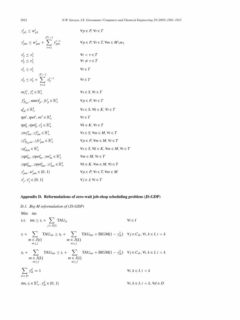
ppendix D. Reformulations of zero-wait job-shop scheduling problem (JS-GDP)
.1. Big-M reformulation of (JS-GDP)
Min ms
s.t. ms≥ ti +∑
j ∈ J(i)
TAUij ∀i ∈ I
ti +∑
m ∈ J(i)m≤j
TAUim ≤ tk +∑
m ∈ J(k)m≤j
TAUkm + BIGM(1 − y1ik) ∀j ∈ Cik, ∀i, k ∈ I, i < k
tk +∑
m ∈ J(k)m≤j
TAUkm ≤ ti +∑
m ∈ J(i)m≤j
TAUim + BIGM(1 − y2ik) ∀j ∈ Cik, ∀i, k ∈ I, i < k
∑d ∈ D
ydik = 1 ∀i, k ∈ I, i < k
ms, ti ∈R1+, ydik ∈ 0, 1 ∀i, k ∈ I, i < k, ∀d ∈ D

N.W. Sawaya, I.E. Grossmann / Computers and Chemical Engineering 29 (2005) 1891–1913 1913
D.2. Convex hull reformulation of (JS-GDP)
Min ms
s.t. ms≥ ti +∑
j ∈ J(i)
TAUij ∀i ∈ I
tn =∑d ∈ D
vdnik ∀i, k ∈ I, i < k, ∀n ∈ I, n = i ∨ k
v1iik − v1
kik ≤
∑m ∈ J(k)
m<j
TAUkm −∑
m ∈ J(i)m≤j
TAUim
y1
ik ∀j ∈ Cik, ∀i, k ∈ I, i < k
v2kik − v2
iik ≤
∑m ∈ J(k)
m<j
TAUim −∑
m ∈ J(i)m≤j
TAUkm
y2
ik ∀j ∈ Cik, ∀i, k ∈ I, i < k
vdnik ≤ UBd
ikydik ∀i, k ∈ I, i < k, ∀n ∈ I, n = i ∨ k∑
d ∈ D
ydik = 1 ∀i, k ∈ I, i < k
ms, ti ∈R1+, ydik ∈ 0, 1 ∀i, k ∈ I, i < k, ∀d ∈ D
R
B hull
B ting
B
B
B ageton,
C dis-
F n
G de-ds.),
G dis-
G ming:
H ing
H
J odel
L eral-
N
R tech-
S for
T
T ms
V dis-rmu-
W
eferences
alas, E. (1998). Disjunctive programming: Properties of the convexof feasible points.Invited paper in Discrete Applied Mathematics, 89,1–44.
alas, E., Ceria, S., & Cornuejols, G. (1993). A lift-and-project cutplane algorithm for mixed 0–1 programs.Mathematical Programming,58(3), 295–324.
azarra, M. S., & Shetty, C. M. (1979).Non-linear programming: Theoryand algorithms. John Wiley & Sons.
iegler, L., Grossmann, I. E., & Westerberg, A. W. (1997).Systematicmethods of chemical process design. Prentice Hall.
rooke A., Kendrick D., Meeruas A., & Raman R., GAMS languguide, Version 98, GAMS Development Corporation, WashingD.C.
eria, S., & Soares, J. (1999). Convex programming forjunctive optimization. Mathematical Programming, 86(3), 595–614.
letcher, R. (1987).Practical methods of optimization (2nd ed.). JohWiley & Sons.
rossmann, I. E., Westerberg, A. W., & Biegler, L. T. (1987). Retrofitsign of chemical processes. In G. V. Reklaitis & H. D. Spriggs (EProceedings of foundations of computer aided process operations (p.403). Elsevier.
rossmann, I. E. (2002). Review of non-linear mixed-integer andjunctive programming techniques.Optimization and Engineering, 3,227–252.
rossmann, I. E., & Lee, S. (2003). Generalized disjunctive programNonlinear convex hull relaxation and algorithms.Computational Op-timization and Applications, 26, 83–100.
ifi, M. (1998). Exact algorithms for the guillotine strip cutting/packproblem.Computers and Operations Research, 25(11), 925–940.
ooker, J. (2000).Logic-based methods for optimization: Combining op-timization and constraint satisfaction. John Wiley & Sons.
ackson, J., & Grossmann, I. E. (2002). High-Level optimization mfor the retrofit planning of process networks.Industrial Engineeringand Chemical Research, 41, 3762–3770.
ee, S., & Grossmann, I. E. (2000). New algorithms for nonlinear genized disjunctive programming.Computers and Chemical Engineering,24, 2125–2141.
emhauser, G. L., & Wolsey, L. A. (1999).Integer and combinatorialoptimization. Wiley Interscience.
aman, R., & Grossmann, I. E. (1994). Modeling and computationalniques for logic based integer programming.Computers and ChemicalEngineering, 18(7), 563–578.
tubbs, R., & Mehrotra, S. (1999). A branch-and-cut method0-1 mixed convex programming.Mathematical Programming, 86,515–532.
awarmalani, M., & Sahinidis, N. V. (2002).Convexification and globaloptimization in continuous and mixed-integer nonlinear programming.Dordrecht: Kluwer Academic Publishers.
urkay, M., & Grossmann, I. E. (1996). Logic-based MINLP algorithfor the optimal synthesis of process networks.Computers and Chem-ical Engineering, 20(8), 959–978.
ecchietti, A., Lee, S., & Grossmann, I. E. (2003). Modeling ofcrete/continuous optimization problems: Characterization and folation of disjunctions and their relaxations.Computers and ChemicalEngineering, 27, 433–448.
illiams, H. P. (1985).Model building in mathematical programming.John Wiley & Sons.