Ann Univ Ferrara (2013) 59:141–158DOI 10.1007/s11565-012-0169-1

The fractional Hankel transform of certain tempereddistributions and pseudo-differential operators

Akhilesh Prasad · V. K. Singh

Received: 22 March 2012 / Accepted: 18 November 2012 / Published online: 18 December 2012© Università degli Studi di Ferrara 2012

Abstract A brief introduction to the fractional Hankel transform and its basic prop-erties is given.The fractional Hankel transform of tempered distributions is studied.A pseudo-differential operator involving fractional Hankel transform is introducedand some of its properties including boundedness are investigated in Gs,2

μ (I ).

Keywords Fractional Hankel transform · Hankel transform · Bessel operator ·Pseudo-differential operator

Mathematics Subject Classification (2000) 46F12 · 47G30

1 Introduction

The Hankel transform, like the Fourier, fractional Fourier, Fresnel, Fresnel–Fourier andthe Laplace transform, is a widely applicable mathematical tool in Physics and otherfields. For example, the zero-order Hankel transform describes the diffraction effectof axially symmetric light beam in free space, and the high order Hankel transformsare usually used in the analysis of laser cavity with circular mirrors [3,13]. A detailedaccount of the properties of the Fourier transform, fractional Fourier transform, Fresneltransform and Fourier–Fresnel transform have been discussed in [3,7,8,10,12] and[14] respectively.

A. Prasad (B) · V. K. SinghDepartment of Applied Mathematics, Indian School of Mines,Dhanbad, 826004, Indiae-mail: apr_bhu@yahoo.com

V. K. Singhe-mail: vks_ism@yahoo.com

123

142 Ann Univ Ferrara (2013) 59:141–158

The conventional Hankel transform of a function ϕ ∈ L1(I ), I = (0,∞), isdefined by

ϕ̂(y) = (hμϕ

)(y) =

∫ ∞

0(xy)1/2 Jμ(xy)ϕ(x)dx (0 < y < ∞), (1.1)

where Jμ is the Bessel function of the first kind of order μ. If ϕ̂ ∈ L1(I ), then theinversion formula of Hankel transform is given by

ϕ(x) =(

h−1μ ϕ̂

)(x) =

∫ ∞

0(xy)1/2 Jμ(xy)ϕ̂(y)dy (0 < x < ∞). (1.2)

The fractional Hankel transform is a generalization of the conventional Hankeltransform in the fractional order and is effectively used in the design of lens, analysisof laser cavity study of wave propagation in quadratic refractive index medium whenthe system is axially symmetric. The earliest work on the fractional Hankel transformwas published by Namias [11] in 1980. Recently it is becoming of importance invarious applications in optics [3,13]. Kerr [5] has developed a theory of fractionalpowers of Hankel transforms in the Zemanian spaces. We define the one dimensionalfractional Hankel transform with parameter α of ϕ(x) for μ ≥ −1/2 and 0 < α < π ,denoted by (hαμϕ)(y) = ϕ̂αμ(y) as:

ϕ̂αμ(y) = (hαμϕ)(y) =∫ ∞

0K αμ(x, y)ϕ(x)dx, (1.3)

where the kernel

K αμ(x, y) =

{Cα,μe

−i2 (x

2+y2) cot α(xy cscα)12 Jμ(xy cscα) if α �= π

2

(xy)1/2 Jμ(xy) if α = π2 ,

and

Cα,μ = exp[i(1 + μ)(π2 − α)]sin α

.

As per Namias [11, p. 190], we have defined the inverse fractional Hankel transformfor ϕ(x) ∈ L1(I ) as:

ϕ(x) = ((hαμ)−1ϕ̂)(x) =

∫ ∞

0K αμ(x, y)(hαμϕ)(y)dy, (1.4)

where

K αμ(x, y) = exp[−i(1 + μ)(

π

2− α)]e i

2 (x2+y2) cot α(xy cscα)

12 Jμ(xy cscα)

= C∗α,μe

i2 (x

2+y2) cot α(xy cscα)12 Jμ(xy cscα),

123

Ann Univ Ferrara (2013) 59:141–158 143

C∗α,μ = exp[−i(1 + μ)(

π

2− α)]

= Cα,μ sin α,

and

h0μϕ = hπμϕ = ϕ, ϕ ∈ Hμ(I ),

hα+2πμ ϕ = hαμϕ, α ∈ R, ϕ ∈ Hμ(I ).

The purpose of the present paper is to derive certain important properties of the frac-tional Hankel transform. Fractional Hankel transform is studied on Zemanian spaceHμ(I ) and tempered distributions space H ′

μ(I ). A pseudo-differential operator involv-ing fractional Hankel transform is introduced and some of its properties includingboundedness are investigated in Gs,2

μ (I ). We shall assume that thoughout of this paperμ ≥ −1/2 and α as above.

2 Properties of fractional Hankel transform

Zemanian [1, p. 129] introduced the function space Hμ(I ) consisting of all complexvalued infinitely differentiable function ϕ defined on I = (0,∞), satisfying

Γμ

m,k(ϕ) = supx∈I

∣∣∣xm(x−1 D)

k[x−μ−1/2ϕ(x)]∣∣∣ < ∞, ∀ μ ∈ R,m, k ∈ N0. (2.1)

If f (x) is a locally integrable function on I such that f (x) is of slow growth as x → ∞and xμ+1/2 f (x) is locally integrable on 0 < x < 1, then f (x) generates a regulargeneralized function f (x) on H ′

μ(I ) by

< f, ϕ >=∫ ∞

0f (x)ϕ(x)dx, ϕ ∈ Hμ(I ).

Proposition 2.1 Let K αμ(x, y) be the kernel of fractional Hankel transform, then

�rμ,x K α

μ(x, y) = (−(y cscα)2)r K αμ(x, y) ∀r ∈ N0.

Proof Since

K αμ(x, y) = Cα,μe

−i2 (x

2+y2) cot α(xy cscα)12 Jμ(xy cscα),

d

dxK αμ(x, y) = Cα,μ

d

dx

[e

−i2 (x

2+y2) cot α(xy cscα)12 Jμ(xy cscα)

]

123

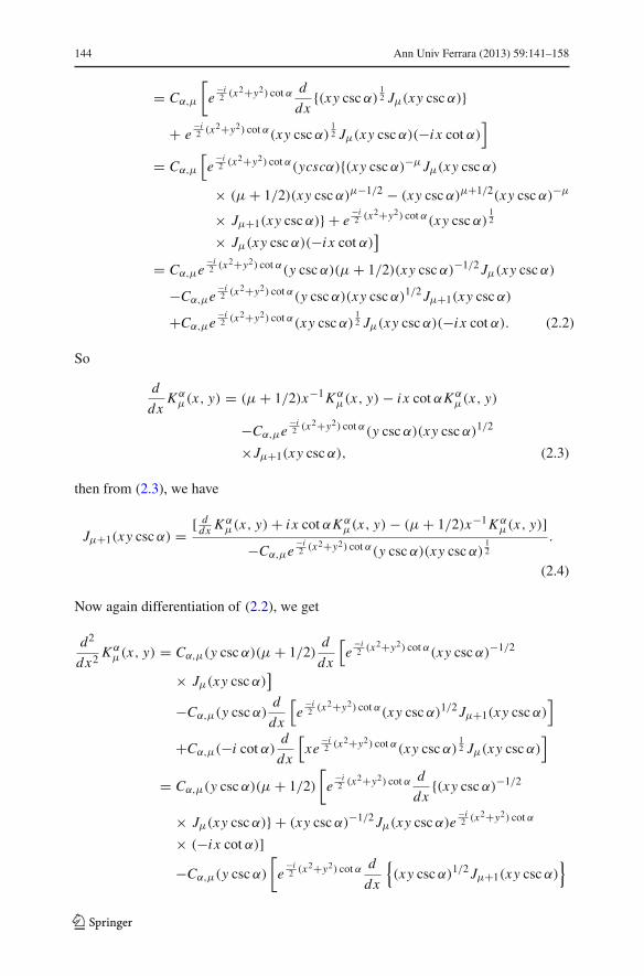
144 Ann Univ Ferrara (2013) 59:141–158

= Cα,μ

[e

−i2 (x

2+y2) cot α d

dx{(xy cscα)

12 Jμ(xy cscα)}

+ e−i2 (x

2+y2) cot α(xy cscα)12 Jμ(xy cscα)(−i x cot α)

]

= Cα,μ[e

−i2 (x

2+y2) cot α(ycscα){(xy cscα)−μ Jμ(xy cscα)

× (μ+ 1/2)(xy cscα)μ−1/2 − (xy cscα)μ+1/2(xy cscα)−μ

× Jμ+1(xy cscα)} + e−i2 (x

2+y2) cot α(xy cscα)12

× Jμ(xy cscα)(−i x cot α)]

= Cα,μe−i2 (x

2+y2) cot α(y cscα)(μ+ 1/2)(xy cscα)−1/2 Jμ(xy cscα)

−Cα,μe−i2 (x

2+y2) cot α(y cscα)(xy cscα)1/2 Jμ+1(xy cscα)

+Cα,μe−i2 (x

2+y2) cot α(xy cscα)12 Jμ(xy cscα)(−i x cot α). (2.2)

So

d

dxK αμ(x, y) = (μ+ 1/2)x−1 K α

μ(x, y)− i x cot αK αμ(x, y)

−Cα,μe−i2 (x

2+y2) cot α(y cscα)(xy cscα)1/2

×Jμ+1(xy cscα), (2.3)

then from (2.3), we have

Jμ+1(xy cscα) = [ ddx K α

μ(x, y)+ i x cot αK αμ(x, y)− (μ+ 1/2)x−1 K α

μ(x, y)]−Cα,μe

−i2 (x

2+y2) cot α(y cscα)(xy cscα)12

.

(2.4)

Now again differentiation of (2.2), we get

d2

dx2 K αμ(x, y) = Cα,μ(y cscα)(μ+ 1/2)

d

dx

[e

−i2 (x

2+y2) cot α(xy cscα)−1/2

× Jμ(xy cscα)]

−Cα,μ(y cscα)d

dx

[e

−i2 (x

2+y2) cot α(xy cscα)1/2 Jμ+1(xy cscα)]

+Cα,μ(−i cot α)d

dx

[xe

−i2 (x

2+y2) cot α(xy cscα)12 Jμ(xy cscα)

]

= Cα,μ(y cscα)(μ+ 1/2)

[e

−i2 (x

2+y2) cot α d

dx{(xy cscα)−1/2

× Jμ(xy cscα)} + (xy cscα)−1/2 Jμ(xy cscα)e−i2 (x

2+y2) cot α

× (−i x cot α)]

−Cα,μ(y cscα)

[e

−i2 (x

2+y2) cot α d

dx

{(xy cscα)1/2 Jμ+1(xy cscα)

}

123

Ann Univ Ferrara (2013) 59:141–158 145

+ (xy cscα)1/2 Jμ+1(xy cscα)e−i2 (x

2+y2) cot α(−i x cot α)]

−Cα,μ(i cot α)

[xe

−i2 (x

2+y2) cot α d

dx

{(xy cscα)1/2 Jμ(xy cscα)

}

+ (xy cscα)1/2 Jμ(xy cscα){

xe−i2 (x

2+y2) cot α(−i x cot α)

+ e−i2 (x

2+y2) cot α}]

= (μ2 − 1/4)x−2 K αμ(x, y)− (2μ+ 2)i cot αK α

μ(x, y)− (y cscα)2

×K αμ(x, y)− x2cot2 αK α

μ(x, y)+ 2Cα,μ(y cscα)(i x cot α)

×e−i2 (x

2+y2) cot α(xy cscα)1/2 Jμ+1(xy cscα).

Using (2.4), we have

d2

dx2 K αμ(x, y) = −

(1 − 4μ2

4x2

)K αμ(x, y)− i cot αK α

μ(x, y)+ x2cot2 αK αμ(x, y)

−2i x cot αd

dxK αμ(x, y)− (y cscα)2 K α

μ(x, y).

Now, we have

[d2

dx2 + 2i x cot αd

dx+

(1 − 4μ2

4x2

)+ i cot α − x2 cot2 α

]K αμ(x, y)

= −(y cscα)2 K αμ(x, y).

Therefore

�μ,x K αμ,x (x, y) = −(y cscα)2 K α

μ(x, y), (2.5)

where

�μ,x =[

d2

dx2 + 2i x cot αd

dx+

(1 − 4μ2

4x2

)+ i cot α − x2 cot2 α

]. (2.6)

Similarly by using (2.5)

�2μ,x K α

μ(x, y) = �μ,x�μ,x K αμ(x, y)

= �μ,x (−(y cscα)2)K αμ(x, y)

= (−(y cscα)2)�μ,x K αμ(x, y)

= (−(y cscα)2)2 K αμ(x, y).

Continuing in this way, we get

�rμ,x K α

μ(x, y) = (−(y cscα)2)r K αμ(x, y), ∀r ∈ N0. (2.7)

123

146 Ann Univ Ferrara (2013) 59:141–158

We now introduce a new function space Hμ,α(I ). �Definition 2.1 Test function space Hμ,α(I ).

The space Hμ,α(I ), is defined as follows: ϕ is member of Hμ,α(I ) if and only if it iscomplex valued C∞− function on I and for every choice of m and k of non-negativeintegers, it satisfies

ϒαm,k(ϕ) = supx∈I

∣∣∣xm�k

μ,xϕ(x)∣∣∣ < ∞, (2.8)

where

�μ,x =[

d2

dx2 + 2i x cot αd

dx+

(1 − 4μ2

4x2

)+ i cot α − x2 cot2 α

], (2.9)

and

�kμ,x = x−2k

2k∑

r=0

(2k∑

l=0

al x2l

) (x−1 d

dx

)r

,

where the constants al depend only onμ and parameter α. The topology over Hμ,α(I )is generated by the family {ϒαm,k}m,k∈N0 of seminorms.

Clearly for α = π2 , Hμ,α(I ) = Hμ(I ), this shown by Pathak [9]. But if α �= π

2 ,

the two spaces Hμ,α(I ) and Hμ(I ) are independent as shown below:It can be easily seen that

xm+2k�kμ,xϕ(x) =

2k∑

r=0

(2k∑

l=0

al xm+2l

)(x−1 d

dx

)r

x−μ−1/2[xμ+1/2ϕ(x)

].

If xμ+1/2ϕ(x) ∈ Hμ(I ), then

supx∈I

∣∣∣xm+2k�k

μ,xϕ(x)∣∣∣

=2k∑

r=0

2k∑

l=0

al supx∈I

∣∣∣∣xm+2l

(x−1 d

dx

)r

x−μ−1/2[xμ+1/2ϕ(x)

]∣∣∣∣ < ∞, ∀ m, l, r ∈ N0.

So the right-hand side is in Hμ(I ). Therefore

supx∈I

∣∣∣xm+2k�k

μ,xϕ(x)∣∣∣ < ∞, ∀ m, k ∈ N0,

this implies that ϕ(x) ∈ Hμ,α(I ).

123

Ann Univ Ferrara (2013) 59:141–158 147

Proposition 2.2 For all ϕ ∈ Hμ(I ), we have

< �rμ,x K α

μ(x, y), ϕ(x) >=< K αμ(x, y), (�∗

μ,x )rϕ(x) >,

where�∗μ,x =

[d2

dx2 − 2i x cot α ddx +

(1−4μ2

4x2

)− i cot α − x2 cot2 α

]. We call�μ,x

and �∗μ,x as fractional Bessel operator with parameter α. We see that for α = π

2then �μ,x = �∗

μ,x = �x , the Bessel operator.

Proof At first we prove

< �μ,x K αμ(x, y), ϕ(x) >=< K α

μ(x, y), (�∗μ,x )ϕ(x) > . (2.10)

Using integration by parts, we have

∫ ∞

0�μ,x K α

μ(x, y)ϕ(x)dx =∫ ∞

0

(d2

dx2 + 2i x cot αd

dx+

(1 − 4μ2

4x2

)

+ i cot α − x2 cot2 α)

K αμ(x, y)ϕ(x)dx

=∫ ∞

0

d2

dx2 (Kαμ(x, y))ϕ(x)dx +

∫ ∞

02i x cot α

× d

dx(K α

μ(x, y))ϕ(x)dx

+∫ ∞

0

(1 − 4μ2

4x2

)K αμ(x, y)ϕ(x)dx

+∫ ∞

0(i cot α − x2 cot2 α)K α

μ(x, y)ϕ(x)dx

=∫ ∞

0K αμ(x, y)

[d2

dx2 − 2i x cot αd

dx+

(1 − 4μ2

4x2

)

− i cot α − x2 cot2 α]ϕ(x)dx

= < K αμ(x, y), (�∗

μ,x )ϕ(x) > .

Therefore

< �μ,x K αμ(x, y), ϕ(x) >=< K α

μ(x, y), (�∗μ,x )ϕ(x) > .

In general, we have

< �rμ,x K α

μ(x, y), ϕ(x) >=< K αμ(x, y), (�∗

μ,x )rϕ(x) > .

�

123

148 Ann Univ Ferrara (2013) 59:141–158

Proposition 2.3 Let ϕ ∈ Hμ(I ), then

(i) hαμ((�∗μ,x )

rϕ)(y) = (−(y cscα)2)r (hαμϕ)(y),

(i i) �rμ,y

(hαμϕ

)(y) = hαμ

(−(x cscα)2)rϕ

)(y),

(i i i) hαμ : Hμ(I ) �−→ Hμ,α(I ), is linear and continuous.

Proof (i) Using Propositions 2.2 and 2.1, we have

hαμ((�∗μ,x )

rϕ)(y) =∫ ∞

0K αμ(x, y)(�∗

μ,x )rϕ(x)dx

=∫ ∞

0(�r

μ,x K αμ(x, y))ϕ(x)dx

= (−(y cscα)2)r∫ ∞

0K αμ(x, y)ϕ(x)dx

= (−(y cscα)2)r (hαμϕ)(y).

�Proof (i i)

�rμ,y

(hαμϕ

)(y) =

∫ ∞

0(�r

μ,y K αμ(x, y))ϕ(x)dx

=∫ ∞

0(−(x cscα)2)r K α

μ(x, y)ϕ(x)dx

=∫ ∞

0K αμ(x, y)(−(x cscα)2)rϕ(x)dx

= hαμ((−(x cscα)2)rϕ

)(y).

�Proof (i i i) Linearity of hαμ is obvious. Let m and k be two non- negative integers(indices). Then by proposition (2.3)(ii), for {ϕ j } j∈N ∈ Hμ,α(I ), we have

supy∈I

∣∣∣ym�kμ,y(h

αμϕ j )(y)

∣∣∣ = supy∈I

∣∣∣ymhαμ((−(x cscα)2)kϕ j

)(y)

∣∣∣ .

Since ϕ j ∈ Hμ(I ), (−(x cscα)2)kϕ j ∈ Hμ(I ). This implies thathαμ

((−(x cscα)2)kϕ j

)(y) ∈ Hμ(I ), hence

ϒαm,k(ϕ j ) = supy∈I

∣∣∣ym�kμ,y(h

αμϕ j )(y)

∣∣∣ −→ 0,

if ϕ j −→ 0 as j −→ α in Hμ,α(I ). This implies continuity of hαμ. �

123

Ann Univ Ferrara (2013) 59:141–158 149

Table 1 Fractional Hankel transform of some functions

f (x) hαμ f (x)

1 ϕ(cx)Cα,μ

c e−i2 y2 cot αhμ

(

e−i2

z2

c2 cot αϕ

)( y cscα

c), c > 0

2 ϕ(x)x

Cα,μ2μ (y cscα)

[1

Cα,μ−1(hαμ−1ϕ)(y)+ 1

Cα,μ+1(hαμ+1ϕ)(y)

]

3 ddx ϕ(x)

Cα,μ4μ (y cscα)

[1

Cα,μ+1(2μ− 1)(hαμ+1ϕ)(y)− 1

Cα,μ−1(2μ+ 1)(hαμ−1ϕ)(y)

]+

i cot α(hαμ(xϕ))(y)

4 xμ+1/2

e−i2 x2 cot α

H(c − x) Cα,μe−i2 y2 cot α

(y cscα)−1/2cμ+1 Jμ+1(cy cscα)

5 δ(x − c) Kαμ(c, y), c > 0.

Proposition 2.4 (Parseval’s identity for fractional Hankel transform) If ϕ,

ψ ∈ Hμ(I ), we have the equalities

∫ ∞

0ϕ(x)ψ(x)dx = sin α

∫ ∞

0(hαμϕ)(y)(h

αμψ)(y)dy,

and

∫ ∞

0|ϕ(x)|2 dx = sin α

∫ ∞

0

∣∣(hαμϕ)(y)∣∣2

dy.

2.1 Further properties of the fractional Hankel transform:

In Table 1, we list a number of additional useful properties of the fractional Hankeltransform, which are extension of the corresponding properties of the Hankel trans-form.

3 The fractional Hankel transform of tempered distributions

3.1 Relation between fractional Hankel transform and Hankel transform:

Since

(hαμϕ)(y) =∫ ∞

0K αμ(x, y)ϕ(x)dx

= Cα,μ

∫ ∞

0e

−i2 (x

2+y2) cot α(xy cscα)12 Jμ(xy cscα)ϕ(x)dx

= Cα,μe−i2 y2 cot α

∫ ∞

0(xy cscα)

12 Jμ(xy cscα)e

−i2 x2 cot αϕ(x)dx

= Cα,μe−i2 y2 cot αhμ(e

−i2 x2 cot αϕ)(y cscα). (3.1)

123

150 Ann Univ Ferrara (2013) 59:141–158

Replacing ϕ(x) = ei2 x2 cot αψ(x), in (3.1), we get

hαμ(ei2 x2 cot αψ)(y) = Cα,μe

−i2 y2 cot α(hμψ)(y cscα). (3.2)

Putting y = z sin α, in (3.2) we have

hαμ(ei2 x2 cot αψ)(z sin α) = Cα,μe

−i4 z2sin 2α(hμψ)(z). (3.3)

Theorem 3.1 The fractional Hankel transform is a continuous linear map of Hμ(I )onto itself.

Proof Letϕ(x) ∈ Hμ(I ) ⊂ L1(I ); then using Zemanian’s technique [1], its fractionalHankel transform

ϕ̂αμ(y) = (hαμϕ)(y)

= Cα,μe−i2 y2 cot αhμ(e

−i2 x2 cot αϕ)(y cscα)

= Cα,μe−i2 y2 cot ααμ(y),

where αμ(y) = hμ(e−i2 x2 cot αϕ)(y cscα). Then

(y−1 D

)βy−μ−1/2ϕ̂αμ(y)

=(

y−1 D)β

y−μ−1/2(

Cα,μe−i2 y2 cot ααμ(y)

)

= Cα,μ

β∑

β ′=0

(β

β ′

) (y−1 D

)β ′(e

−i2 y2 cot α)

(y−1 D

)β−β ′(y−μ−1/2αμ(y))

= Cα,μ

β∑

β ′=0

(β

β ′

)(−i cot α)β

′(e

−i2 y2 cot α)

(y−1 D

)β−β ′(y−μ−1/2αμ(y)).

Therefore, as per Koh [4], we have

supy∈I

∣∣∣∣ym

(y−1 D

)βy−μ−1/2ϕ̂αμ(y)

∣∣∣∣ = Cα,μ

β∑

β ′=0

(β

β ′

)(cot α)β

′

× supy∈I

∣∣∣∣y

m(

y−1 D)β−β ′

(y−μ−1/2αμ(y))

∣∣∣∣

< ∞. (3.4)

Henceαμ(y) ∈ Hμ(I ). Thus ϕ̂αμ(y) = (hαμϕ)(y) ∈ Hμ(I ). Also from (1.3) and (1.4),we see that for all ϕ ∈ Hμ(I ),

((hαμ)−1hαμϕ) = ϕ = (hαμ(h

αμ)

−1ϕ).

123

Ann Univ Ferrara (2013) 59:141–158 151

It follows that hαμ is a one-one function of Hμ(I ) onto itself. hαμ is clearly a linear mapof Hμ(I ) onto itself. To show that it is continuous, assume that the sequence {ϕ j } j∈N

converges in Hμ(I ) to zero, then from (3.4) the continuity of the fractional Hankeltransform follows. �Definition 3.1 : The generalized fractional Hankel transform hαμ f of f ∈ H ′

μ(I ) isdefined by

< hαμ f , ϕ >=< f, hαμϕ >, (3.5)

where ϕ ∈ Hμ(I ).

Theorem 3.2 The generalized fractional Hankel transform hαμ is a continuous linearmap of H ′

μ(I ) onto itself.

Proof Since by Theorem 3.1, hαμϕ ∈ Hμ(I ) whenever ϕ ∈ Hμ(I ), the right-handside of (3.5) is well defined. Also, if {ϕ j } j∈N converges in Hμ(I ) to zero, then bycontinuity of the fractional Hankel transform {hαμϕ j } → 0, and so the right-hand sideof (3.5) converges to zero, which in turn implies that {< hαμ f , ϕ j >} → 0 as j → ∞.

Thus hαμ f is continuous on H ′μ(I ). Clearly hαμ f is linear on H ′

μ(I ). Similarly the

inverse fractional Hankel transform (hαμ)−1 f of f ∈ H ′

μ(I ) is defined by

< (hαμ)−1 f , ϕ >=< f, (hαμ)

−1ϕ > . ϕ ∈ Hμ(I ). (3.6)

It can be shown, as in the above, that (hαμ)−1 f ∈ H ′

μ(I ). Thus from (3.5) and (3.6) itfollows that for f ∈ H ′

μ(I ) and ϕ ∈ Hμ(I ),

< f, ϕ >=< hαμ f , (hαμ)−1ϕ >=< f, hαμ(h

αμ)

−1ϕ > .

So that

(hαμ)−1hαμ f = f. (3.7)

Similarly

hαμ(hαμ)

−1 f = f.

Thus hαμ and (hαμ)−1 are one-one map of H ′

μ(I ) onto itself. �

4 Pseudo-differential operator hαμ,a

A linear partial differential operator A(x, (�∗μ,x )) on I is given by

A(x, (�∗μ,x )) =

m∑

r=0

ar (x)(�∗μ,x )

r , (4.1)

123

152 Ann Univ Ferrara (2013) 59:141–158

where the cofficient ar (x) are functions defined on I and �∗μ,x is the same as in

Proposition 2.2. If we replace (�∗μ,x )

r in (4.1) by monomial (−(y cscα)2)r in I ,then we obtain the so called symbol

A(x, y) =m∑

r=0

ar (x)(−(y cscα)2)r . (4.2)

In order to get another representation of the operator A(x, (�∗μ,x )), let us take any

function ϕ ∈ Hμ(I ), then by using (1.4) and Proposition 2.3(i), we have

(A(x, (�∗

μ,x ))ϕ)(x) =

m∑

r=0

ar (x)((�∗μ,x )

rϕ)(x)

=m∑

r=0

ar (x)(hαμ)

−1(hαμ(�

∗μ,x )

rϕ)(x)

=m∑

r=0

ar (x)(hαμ)

−1(−(y cscα)2)r (hαμϕ)

)(x)

=∫ ∞

0K αμ(x, y)

(m∑

r=0

ar (x)(−(y cscα)2)r)

ϕ̂αμ(y)dy

=∫ ∞

0K αμ(x, y)A(x, y)ϕ̂αμ(y)dy,

where K αμ(x, y) is the same as in (1.4). If we replace the symbol A(x, y) by more gen-

eral symbol a(x, y)which is no longer polynomial in y, we get the pseudo-differentialoperator hαμ,a defined below. For pseudo-differential operator involving Fourier trans-form and fractional Fourier transform we may refer to [6,8] and [2] respectively.

Definition 4.1 Let a be a symbol. Then the pseudo-differential operator hαμ,a associ-ated to a is defined by

(hαμ,aϕ

)(x) =

∫ ∞

0K αμ(x, y)a(x, y)ϕ̂αμ(y)dy,

where ϕ̂αμ(y) as (1.3).

Definition 4.2 Let l ∈ R. Then we define Hl1 to the set of all functions a(x, y) ∈

C∞(I × I ) such that for any two non-negative integers ν and β, there exists a positiveconstant Cl,ν,β such that

∣∣∣∣∣

(x−1 d

dx

)ν (y−1 d

dy

)βa(x, y)

∣∣∣∣∣≤ Cl,ν,β(1 + y)l−β, (4.3)

where x, y ∈ I .

123

Ann Univ Ferrara (2013) 59:141–158 153

Zemanian[1, p. 141] and Pathak [9, p. 295] have given the following result(−1)m+n xm

(x−1 d

dx

)nx−μ−1/2(hμϕ)(x)

=∫ ∞

0y2μ+m+2n+1

(y−1 d

dy

)m (y−μ−1/2ϕ(y)

)

×(xy)−(μ+n) Jμ+m+n(xy)dy, ∀,m, n ∈ N0. (4.4)

Theorem 4.1 The pseudo-differential operator hαμ,a is a continuous linear mappingof Hμ(I ) into itself.

Proof Let ϕ ∈ Hμ(I ). Then for any two non-negative integers m and k, we need onlyprove that

supx∈I

∣∣∣xm(x−1 D)kx−μ−1/2(hαμ,aϕ)(x)

∣∣∣ < ∞.

Following the technique of Proof of Theorem 3.1, we have

xm(x−1 D)kx−μ−1/2(hαμ,aϕ)(x)

= xm(x−1 D)kx−μ−1/2

∫ ∞

0K αμ(x, y)a(x, y)ϕ̂αμ(y)dy

= xm(x−1 D)kx−μ−1/2C∗

α,μei2 x2 cot αhμ

(e

i2 y2 cot αa(x, y)ϕ̂αμ(y)

)(x cscα)

= xmC∗α,μ

k∑

ν=0

(k

ν

)(x−1 D)

k−νe

i2 x2 cot α

×(x−1 D)νx−μ−1/2hμ

(e

i2 y2 cot αa(x, y)ϕ̂αμ(y)

)(x cscα).

Now

xm(x−1 D)kx−μ−1/2(hαμ,aϕ)(x)

= (−1)−(m+ν)C∗α,μ

k∑

ν=0

(k

ν

)(i cot α)k−νe

i2 x2 cot α(−1)m+νxm

×(x−1 D)νx−μ−1/2hμ

(e

i2 y2 cot αa(x, y)ϕ̂αμ(y)

)(x cscα).

Applying the Zemanian’s result from (4.4), we have

= C∗α,μ

k∑

ν=0

(k

ν

)(i cot α)k−νe

i2 x2 cot α(sin α)m−2ν−μ−1/2

×∫ ∞

0y2μ+m+2ν+1(y−1 D)m

(y−μ−1/2e

i2 y2 cot αa(x, y)ϕ̂αμ(y)

)

×(xy cscα)−(μ+ν) Jμ+m+ν(xy cscα)dy

123

154 Ann Univ Ferrara (2013) 59:141–158

= C∗α,μ

k∑

ν=0

(k

ν

)(i cot α)k−νe

i2 x2 cot α(sin α)m−2ν−μ−1/2

×∫ ∞

0y2μ+m+2ν+1

m∑

s=0

m−s∑

t=0

(m

s

)(m − s

t

)(y−1 D)

m−s−te

i2 y2 cot α

×(y−1 D)ta(x, y)(y−1 D)s

(y−μ−1/2ϕ̂αμ(y)

)(xy cscα)−(μ+ν) Jμ+m+ν(xy cscα)dy.

Suppose N is an integer no less than 2μ+ m + 2ν + 1 and using (4.3), then we have

supx∈I

∣∣∣xm(x−1 D)kx−μ−1/2(hαμ,aϕ)(x)

∣∣∣

≤k∑

ν=0

(k

ν

)(cot α)k−ν(sin α)m−2ν−μ−1/2

m∑

s=0

m−s∑

t=0

(m

s

)(m − s

t

)(cot α)m−s−t

×supx,y∈I

∣∣∣(xy cscα)−(μ+ν) Jμ+m+ν(xy cscα)∣∣∣

×supy∈I (1 + y)N+2∣∣∣(y−1 D)s y−μ−1/2ϕ̂αμ(y)

∣∣∣ |(y−1 D)ta(x, y)|

∫ ∞

0

dy

(1 + y)2

≤k∑

ν=0

(k

ν

)(cot α)k−ν(sin α)m−2ν−μ−1/2

m∑

s=0

m−s∑

t=0

(m

s

)(m − s

t

)(cot α)m−s−t

×Aμ,α Cl,t supy∈I

∣∣∣(1 + y)N+2+l−t (y−1 D)s y−μ−1/2ϕ̂αμ(y)

∣∣∣ ,

where 0 < supx,y∈I

∣∣(xy cscα)−(μ+ν) Jμ+m+ν(xy cscα)∣∣ ≤ Aμ,α .

Using binomial formula and Theorem 3.1, we have

supx∈I

∣∣∣xm(x−1 D)

kx−μ−1/2(hαμ,aϕ)(x)

∣∣∣ < ∞.

�

5 Boundedness of pseudo-differential operator

In this section we assume that the symbol b(x, y) = a(x, y)(xy cscα)1/2 Jμ(xy cscα)satisfies the following condition instead of (4.3). For given l ∈ R, assume that

(1 + x)q∣∣∣∣∣

(x−1 d

dx

)ν (y−1 d

dy

)βb(x, y)

∣∣∣∣∣≤ Dl,ν,β,q,α(1 + y)l−β, (5.1)

where x, y ∈ I, Dl,ν,β,q,α > 0 and q, ν, β ∈ N0.

The class of all such symbols is denoted by Hl .

123

Ann Univ Ferrara (2013) 59:141–158 155

Definition 5.1 A tempered distributions ϕ belongs to the Sobolev type spaceGs,2μ , s, μ ∈ R, if its fractional Hankel transform (hαμϕ) corresponds to a locally

integrable function (hαμϕ)(y) over I = (0,∞) such that

||ϕ||Gs,2μ (I ) =

(∫ ∞

0

∣∣∣(1 + y2)s/2(hαμϕ)(y)∣∣∣2

dy

) 12

. (5.2)

Lemma 5.1 For any symbol b(x, y) ∈ Hl , l ∈ R and k ∈ N0, there exists a positiveconstant Cl such that

|b̂αμ(y, ξ)| ≤ Cl(1 + ξ)l(1 + y2 csc2 α)−k/2. (5.3)

Proof Since

b̂αμ(y, ξ) =∫ ∞

0K αμ(x, y)b(x, ξ)dx,

so that,

(1 + y2 csc2 α)k b̂αμ(y, ξ) =∫ ∞

0K αμ(x, y)(1 −�∗

μ,x )kb(x, ξ)dx, (5.4)

∀y, ξ ∈ I, k ∈ N0. Then we have

(1 −�∗μ,x )

kb(x, ξ) =k∑

r=0

(k

r

)(−1)r (�∗

μ,x )r b(x, ξ)

=k∑

r=0

(k

r

)(−1)r x−2r

2r∑

n=0

⎛

⎝2r∑

k=0

mk x2k

⎞

⎠(

x−1 d

dx

)nb(x, ξ)

=k∑

r=0

(k

r

)(−1)r x−2r

2r∑

n=0

⎛

⎝2r∑

k=0

mk x2k

⎞

⎠ Dl,n,q,α(1 + ξ)l (1 + x)−q .

So

|(1−�∗μ,x )

kb(x, ξ)| ≤k∑

r=0

(k

r

) 2r∑

n=0

(2r∑

k=0

mk

)

Dl,n,q,α(1+ξ)l(1+x)2k−2r−q . (5.5)

Hence by (5.4) and (5.5), we get

|(1 + y2 csc2 α)k ||b̂αμ(y, ξ)| ≤ |Cα,μ|k∑

r=0

(k

r

) 2r∑

n=0

(2r∑

k=0

mk

)

Dl,n,q,α(1 + ξ)l

×∫ ∞

0(1 + x)2k−2r−qdx .

123

156 Ann Univ Ferrara (2013) 59:141–158

Since x- integral is convergent for sufficient large value of q, there exists a constantCl > 0 such that

|b̂αμ(y, ξ)| ≤ Cl(1 + ξ)l(1 + y2 csc2 α)−k/2.

�Proposition 5.1 For any symbol b(x, y) = a(x, y)(xy cscα)

12 Jμ(xy cscα) ∈

Hl , l ∈ R, the associated operator (hαμ,a ϕ) admits the representation

(hαμ,a ϕ) = C∗α,μ e

i2 x2 cot α

∫ ∞

0K αμ(x, y)

[∫ ∞

0e

i2 ξ

2 cot α b̂αμ(y, ξ)ϕ̂αμ(ξ)dξ

]dy,

(5.6)

where ϕ ∈ Hμ(I ) and all involved integrals are convergent.

Proof In order to case establish its validity, we first note that

(1 + ξ)l ≤ Dl(1 + ξ2)l/2, ξ ∈ I, (5.7)

where Dl = max(1, 2l/2). Hence from (5.3)

|b̂αμ(y, ξ)| ≤ Cl Dl(1 + ξ2)l/2(1 + y2 csc2 α)−k/2. (5.8)

Let

gα(y) =∫ ∞

0e

i2 ξ

2 cot α b̂αμ(y, ξ)ϕ̂αμ(ξ)dξ

is in L1(I ). We now compute its inverse fractional Hankel transform

C∗α,μ

∫ ∞

0e

i2 (x

2+y2) cot α(xy cscα)12 Jμ(xy cscα)

[∫ ∞

0e

i2 ξ

2 cot α b̂αμ(y, ξ)ϕ̂αμ(ξ)dξ

]dy

= e−i2 x2 cot α

C∗α,μ

[C∗α,μ

∫ ∞

0e

i2 (x

2+y2) cot α(xy cscα)12 Jμ(xy cscα)

× {C∗α,μ

∫ ∞

0e

i2 (x

2+ξ2) cot α b̂αμ(y, ξ)ϕ̂αμ(ξ)dξ}dy

]

= e−i2 x2 cot α

C∗α,μ

[C∗α,μ

∫ ∞

0e

i2 (x

2+ξ2) cot αϕ̂αμ(ξ)

× {C∗α,μ

∫ ∞

0e

i2 (x

2+y2) cot α(xy cscα)12 Jμ(xy cscα)b̂αμ(y, ξ)dy}dξ

]

= e−i2 x2 cot α

C∗α,μ

[C∗α,μ

∫ ∞

0e

i2 (x

2+ξ2) cot αb(x, ξ)ϕ̂αμ(ξ)dξ

]

123

Ann Univ Ferrara (2013) 59:141–158 157

= e−i2 x2 cot α

C∗α,μ

[C∗α,μ

∫ ∞

0e

i2 (x

2+ξ2) cot α(xξ cscα)12 Jμ(xξ cscα)

× b(x, ξ)

(xξ cscα)12 Jμ(xξ cscα)

ϕ̂αμ(ξ)dξ

]

= e−i2 x2 cot α

C∗α,μ

[C∗α,μ

∫ ∞

0e

i2 (x

2+ξ2) cot α(xξ cscα)12 Jμ(xξ cscα)a(x, ξ)ϕ̂αμ(ξ)dξ

]

= e−i2 x2 cot α

C∗α,μ

[∫ ∞

0K αμ(x, ξ)a(x, ξ)ϕ̂

αμ(ξ)dξ

]

= e−i2 x2 cot α

C∗α,μ

(hαμ,a ϕ)(x).

�Theorem 5.1 Let a(x, y) = b(x,y)

(xy cscα)12 Jμ(xy cscα)

∈ Hl and (hαμ,a ϕ) be associated

operator. Then the following estimate holds true:

||(hαμ,a ϕ)||G0,2μ (I ) ≤ C(α)||ϕ||Gl,2

μ (I ),

where ϕ ∈ Hμ(I ), for a certain constant C = C(α)

Proof We have seen (5.6) the tempered distributions (e−i2 x2 cot αhαμ,a ϕ) has fractional

Hankel transform equal to

(C∗μ,α)

−1hαμ(e−i2 x2 cot αhαμ,a ϕ) = gα(y) =

∫ ∞

0e

−i2 ξ

2 cot α b̂αμ(y, ξ)ϕ̂αμ(ξ)dξ.

Let us set

Uα(y) =∫ ∞

0e

i2 ξ

2 cot α b̂αμ(y, ξ)ϕ̂αμ(ξ)dξ

|Uα(y)| ≤∫ ∞

0|b̂αμ(y, ξ)||ϕ̂αμ(ξ)|dξ.

Using (5.8), we have

|Uα(y)| ≤ Cl Dl

∫ ∞

0(1 + ξ2)l/2(1 + y2 csc2 α)−k/2|ϕ̂αμ(ξ)|dξ

≤ Cl Dl(1 + y2 csc2 α)−k/2∫ ∞

0(1 + ξ2)l/2|ϕ̂αμ(ξ)|dξ.

Let fα(y) = (1 + y2 csc2 α)−k/2 and θα(ξ) = (1 + ξ2)l/2|ϕ̂αμ(ξ)|. If k is sufficient

large, fα ∈ L1(I ) as ϕ̂αμ ∈ Hμ(I ), θα ∈ L2(I ).

123

158 Ann Univ Ferrara (2013) 59:141–158

Then

||Uα(y)||L2(I ) ≤ C(α)||ϕ||Gl,2μ (I )

.

Therefore, using (5.6), we have

||(C∗μ,α)

−1(e−i2 x2 cot αhαμ,a ϕ)||G0,2

μ (I ) = ||(C∗μ,α)

−1hαμ(e−i2 x2 cot αhαμ,a ϕ)||L2(I )

= ||Uα(y)||L2(I )

≤ C(α)||ϕ||Gl,2μ (I )

.

Hence this implies that

||(hαμ,a ϕ)||G0,2μ (I ) ≤ C(α)||ϕ||Gl,2

μ (I ).

This completes the proof of theorem. �Acknowledgments Authors are very thankful to the reviewers for his/ her comments and suggestions.This work was supported by University Grants Commission, Govt. of India, under grant no.F.No.34-145/2008(SR).

References

1. Zemanian, A.H.: Generalized Integral Transformations. Interscience Publishers, New York (1968)2. Prasad, A., Kumar, M.: Product of two generalized pseudo-differential operators involving fractional

Fourier transform. J. Pseudo-Diff. Oper. Appl. 2, 355–365 (2011)3. Sheppard, C.J.R., Larkin, K.G.: Similarity theorems for fractional Fourier transforms and fractional

Hankel transforms. Opt. Commun. 154, 173–178 (1998)4. Koh, E.L.: The n-dimensional distributional Hankel transformation. Can. J. Math. 27, 423–433 (1975)5. Kerr, F.H.: Fractional powers of Hankel transforms in the Zemanian spaces. J. Math. Anal. Appl. 166,

65–83 (1992)6. Feichtinger, H.G., Helffer, B., Lamoureux, M.P., Lerner, N., Toft, J.: Pseudo-Differential Operators.

Quantization and Signals Lectures, C.I.M.E. Summer School, Cetraro (2006)7. Ozaktas, H.M., Kutay, M.A., Zalevsky, Z.: The Fractional Fourier Transform with Applications in

Optics and Signal Processing. Wiley, New York (2000)8. Wong, M.W.: An Introduction to Pseudo-Differential Operators. World Scientific, Singapore (1999)9. Pathak, R.S.: Integral Transforms of Generalized Functions and Their Applications. Gordon and Breach

Publishers, Amsterdam (1997)10. Osipov, V.F.: Bohr-Fresnel Almost-Periodic Functions. University of Saint-Petersbourg, St Petersbourg

(1992)11. Namias, V.: Fractionalization of Hankel transform. J. Inst. Math. Appl. 26, 187–197 (1980)12. Neretin, Y.A.: Lectures on Gaussian Integral Operators and Classical Groups. European Mathematical

Society (2011)13. Zhang, Y., Funaba, T., Tanno, N.: Self-fractional Hankel functions and their properties. Opt. Commun.

176, 71–75 (2000)14. Abzhandadze, Z.L., Osipov, V.F.: Fourier–Fresnel Transform and Some of its Applications. University

of Saint-Petersbourg, St Petersbourg (2000)

123