Tempered Fractional Calculus

International Symposium on Fractional PDEs:

Theory, Numerics and Applications

3–5 June 2013

Mark M. Meerschaert

Department of Statistics and Probability

Michigan State University

mcubed@stt.msu.edu

http://www.stt.msu.edu/users/mcubed

Partially supported by NSF grant DMS-1025486 and NIH grant R01-EB012079.

Abstract

Fractional Calculus has a close relation with Probability. Randomwalks with heavy tails converge to stable stochastic processes,whose probability densities solve space-fractional diffusion equa-tions. Continuous time random walks, with heavy tailed wait-ing times between particle jumps, converge to non-Markovianstochastic limits, whose probability densities solve time-fractionaldiffusion equations. Time-fractional derivatives and integrals ofBrownian motion produce fractional Brownian motion, a usefulmodel in many applications. Fractional derivatives and integralsare convolutions with a power law. Including an exponential termleads to tempered fractional derivatives and integrals. Temperedstable processes are the limits of random walk models where thepower law probability of long jumps is tempered by an exponen-tial factor. These random walks converge to tempered stablestochastic process limits, whose probability densities solve tem-pered fractional diffusion equations. Tempered power law wait-ing times lead to tempered fractional time derivatives, whichhave proven useful in geophysics. Applying this idea to Brown-ian motion leads to tempered fractional Brownian motion, a newstochastic process that can exhibit semi-long range dependence.The increments of this process, called tempered fractional Gaus-sian noise, provide a useful new stochastic model for wind speeddata.

Acknowledgments

Farzad Sabzikar, Statistics and Probability, Michigan State

Boris Baeumer, Maths & Stats, University of Otago, New Zealand

Anna K. Panorska, Mathematics and Statistics, U of Nevada

Parthanil Roy, Indian Statistical Institute, Kolkata

Hans-Peter Scheffler, Math, Universitat Siegen, Germany

Qin Shao, Mathematics, University of Toledo, Ohio

Alla Sikorskii, Statistics and Probability, Michigan State

Yong Zhang, Desert Research Institute, Las Vegas Nevada

New Books

Stochastic Models for Fractional Calculus

Mark M. Meerschaert and Alla Sikorskii

De Gruyter Studies in Mathematics 43, 2012

Advanced graduate textbook

ISBN 978-3-11-025869-1

Mathematical Modeling, 4th Edition

Mark M. Meerschaert

Academic Press, Elsevier, 2013

Advanced undergraduate / beginning graduate textbook

(new sections on particle tracking and anomalous diffusion)

ISBN 978-0-12-386912-8

Continuous time random walks

-

6

X1

X2X3

X4X5

u

u

u

u

u

u

Rd

0tW1 W2 W3 W4 W5

A random particle arrives at location S(n) = X1 + · · · + Xn at

time Tn =W1+ · · ·+Wn. After Nt = max{n ≥ 0 : Tn ≤ t} jumps,

particle location is S(Nt).

CTRW limit theory

If P (Xn > x) ≈ x−α and E(Xn) = 0 then n−1/αS(nu) ⇒ A(u).

The α-stable limit A(u) has pdf p(x, u) with Fourier transform

p(k, u) = euψA(k) and Fourier symbol ψA(k) = (ik)α for 1 < α ≤ 2.

If P (Wn > t) ≈ t−β then n−1/βTnu ⇒ Du. The β-stable limit has

pdf g(t, u) with Laplace transform g(s, u) = e−uψD(s) and Laplace

symbol ψD(s) = sβ for 0 < β < 1.

Inverse process: n−βNnt ⇒ Et = inf{u > 0 : Du > t}, and then

n−β/αS(Nnt) = n−β/αS(nβ ·n−βNnt) ≈ (nβ)−1/αS(nβ ·Et) ⇒ A(Et).

Since Et has a pdf h(u, t) with LT h(u, s) = s−1ψD(s)e−uψD(s),

the CTRW limit A(Et) has pdf

q(x, t) =∫ ∞

0p(x, u)h(u, t)du ≈

∑

uP (A(u) = x|Et = u)P (Et = u).

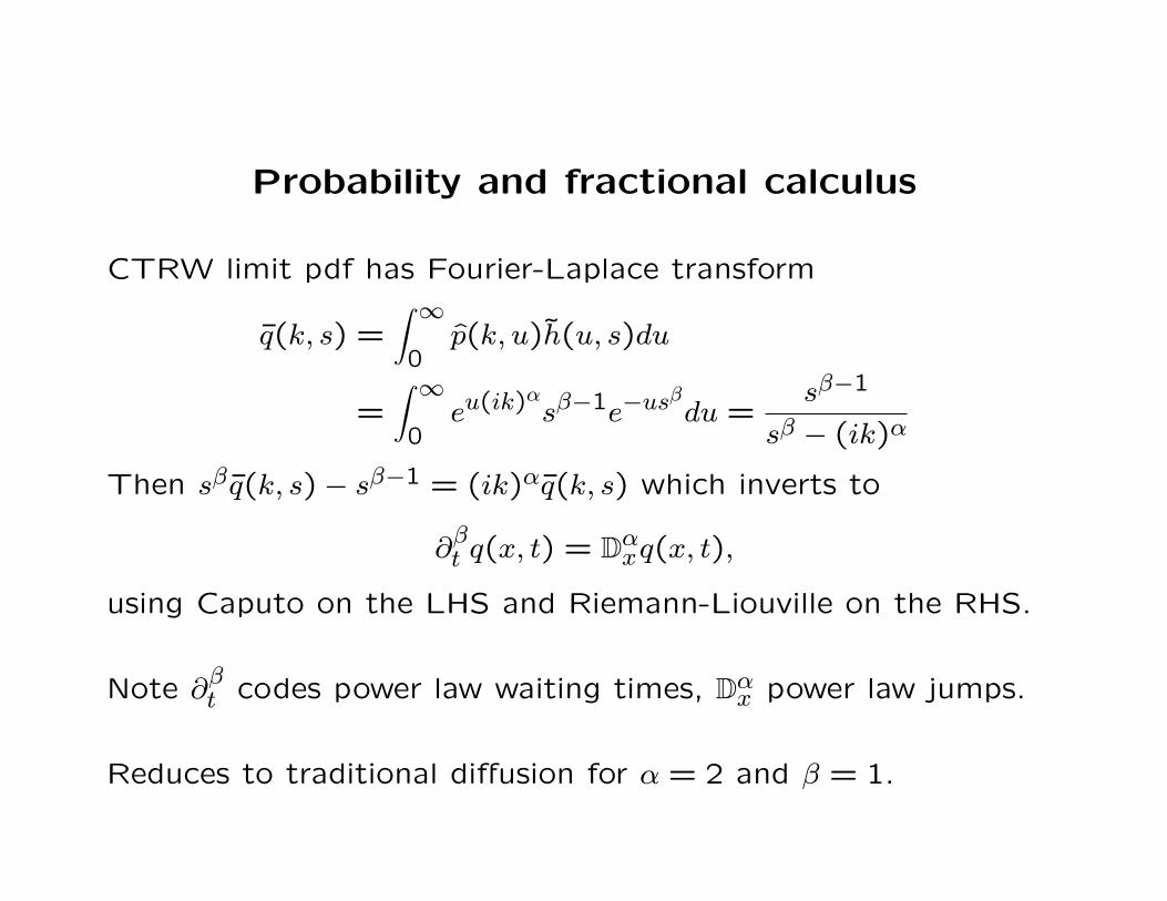
Probability and fractional calculus

CTRW limit pdf has Fourier-Laplace transform

q(k, s) =∫ ∞

0p(k, u)h(u, s)du

=∫ ∞

0eu(ik)

αsβ−1e−us

βdu =

sβ−1

sβ − (ik)α

Then sβq(k, s)− sβ−1 = (ik)αq(k, s) which inverts to

∂βt q(x, t) = D

αxq(x, t),

using Caputo on the LHS and Riemann-Liouville on the RHS.

Note ∂βt codes power law waiting times, D

αx power law jumps.

Reduces to traditional diffusion for α = 2 and β = 1.

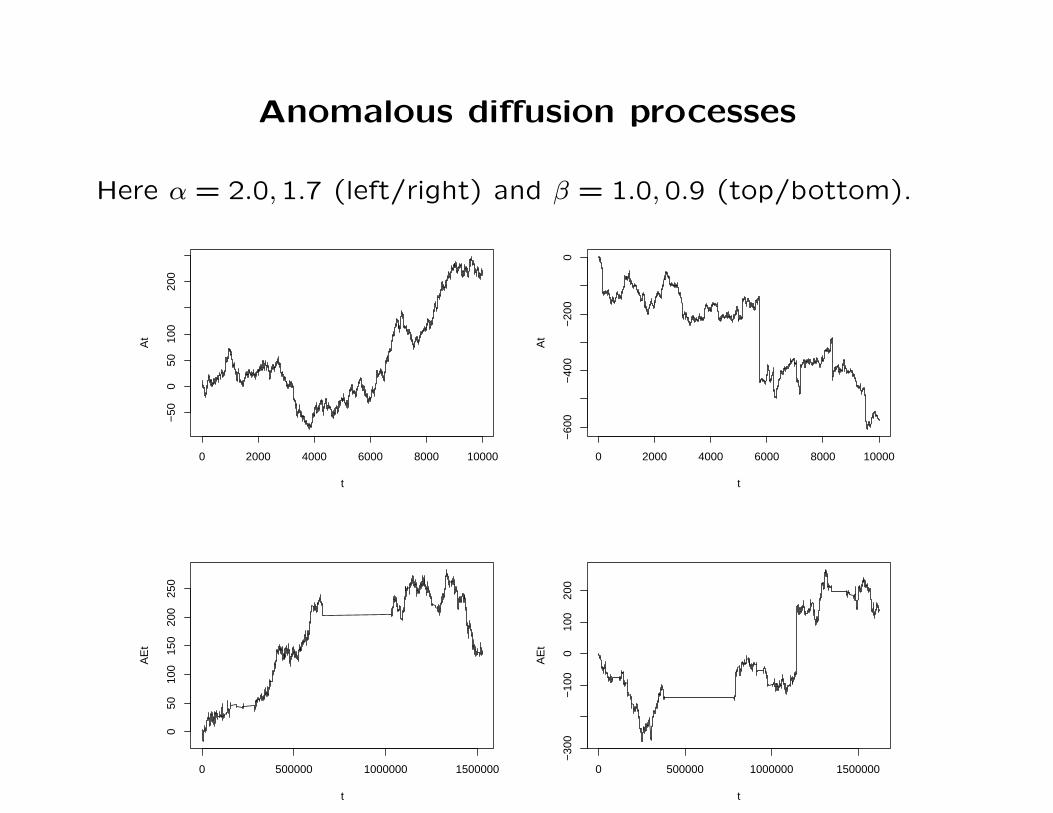
Anomalous diffusion processes

Here α = 2.0,1.7 (left/right) and β = 1.0,0.9 (top/bottom).

0 2000 4000 6000 8000 10000

−50

050

100

200

t

At

0 2000 4000 6000 8000 10000

−60

0−

400

−20

00

t

At

0 500000 1000000 1500000

050

100

150

200

250

t

AE

t

0 500000 1000000 1500000

−30

0−

100

010

020

0

t

AE

t

Tempered fractional calculus

Tempered stable Dt has pdf with LT g(t, u) = e−uψD(s) where the

Laplace symbol ψD(s) = (λ+ s)β − λβ for some λ > 0 (small).

Tempered stable A(u) has pdf with FT p(k, u) = euψA(k) where

the Fourier symbol ψA(k) = (λ+ ik)α− λα− ikαλα−1 with λ > 0.

Again Et has pdf with LT h(u, s) = s−1ψD(s)e−uψD(s), and again

A(Et) has pdf q(x, t) =∫ ∞

0p(x, u)h(u, t)du with FLT

q(k, s) =s−1ψD(s)

ψD(s)− ψA(k)

Then ψD(s)q(k, s)− s−1ψD(s) = ψA(k)q(k, s). Invert to get

∂β,λt q(x, t) = D

α,λx q(x, t).

Tempered jumps P (Xn > x) ≈ x−αe−λx and waiting times.

Space fractional tempered stable

Tempered stable Levy motion with α = 1.2

0 5000 10000−150

−100

−50

0

λ = 0.1

0 5000 10000−200

0

200λ = 0.01

0 5000 10000−500

0

500λ = 0.001

0 5000 10000

−500

0

500

1000λ = 0.0001

Tempered power laws in finance

AMZN stock price changes fit a tempered power law model

P (X > x) ≈ x−0.6e−0.3x for x large

oooooooooooooooooooooooooooooooooooooooooooooooooooooooooooooooooooooooooooooooooooooooooooooooooooooo ooooooooo ooooooo oooooooooooooooooo o o o ooo o ooo

ooo

o

o

o

o

1.5 2.0 2.5 3.0

-8-7

-6-5

-4-3

-2

1.5 2.0 2.5 3.0

-8-7

-6-5

-4-3

-2

ln(x)

ln(P

(X>

x))

1.5 2.0 2.5 3.0

-8-7

-6-5

-4-3

-2

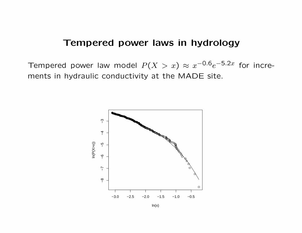
Tempered power laws in hydrology

Tempered power law model P (X > x) ≈ x−0.6e−5.2x for incre-

ments in hydraulic conductivity at the MADE site.

−3.0 −2.5 −2.0 −1.5 −1.0 −0.5

−8

−7

−6

−5

−4

−3

ln(x)

ln(P

(X>

x))

Tempered power laws in atmospheric science

Tempered power law model P (X > x) ≈ x−0.2e−0.01x for daily

precipitation data at Tombstone AZ.

4.0 4.5 5.0 5.5 6.0 6.5

−8

−6

−4

−2

ln(x)

ln(P

(X>

x))

Tempered stable pdf in macroeconomics

data

Den

sity

−0.2 0.0 0.2 0.4

02

46

810

12

One-step BARMA forecast errors for annual inflation rates, and

a tempered stable with α = 1.1 and λ = 12 (rough fit).

Tempered time-fractional diffusion model

Fitted concentration data from a 3-D supercomputer simulation.

ADE fit uses α = 2, β = 1. Without cutoff uses λ = 0.

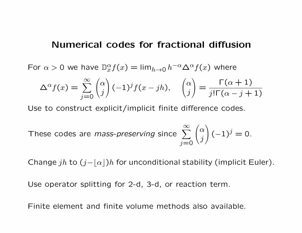
Numerical codes for fractional diffusion

For α > 0 we have Dαxf(x) = limh→0 h

−α∆αf(x) where

∆αf(x) =∞∑

j=0

(

αj

)

(−1)jf(x− jh),

(

αj

)

=Γ(α+1)

j!Γ(α− j +1)

Use to construct explicit/implicit finite difference codes.

These codes are mass-preserving since∞∑

j=0

(

αj

)

(−1)j = 0.

Change jh to (j−⌊α⌋)h for unconditional stability (implicit Euler).

Use operator splitting for 2-d, 3-d, or reaction term.

Finite element and finite volume methods also available.

Numerical example

Exact solution p(x, t) = e−tx3 and numerical approximation to

∂p(x, t)

∂t= d(x)

∂1.8p(x, t)

∂x1.8+ r(x, t)

on 0 < x < 1 with p(x,0) = x3, p(0, t) = 0, p(1, t) = e−t, r(x, t) =

−(1 + x)e−tx3, d(x) = Γ(2.2)x2.8/6.

0

0.05

0.1

0.15

0.2

0.25

0.3

0.35

0.4

0 0.2 0.4 0.6 0.8 1 1.2

Exact CN

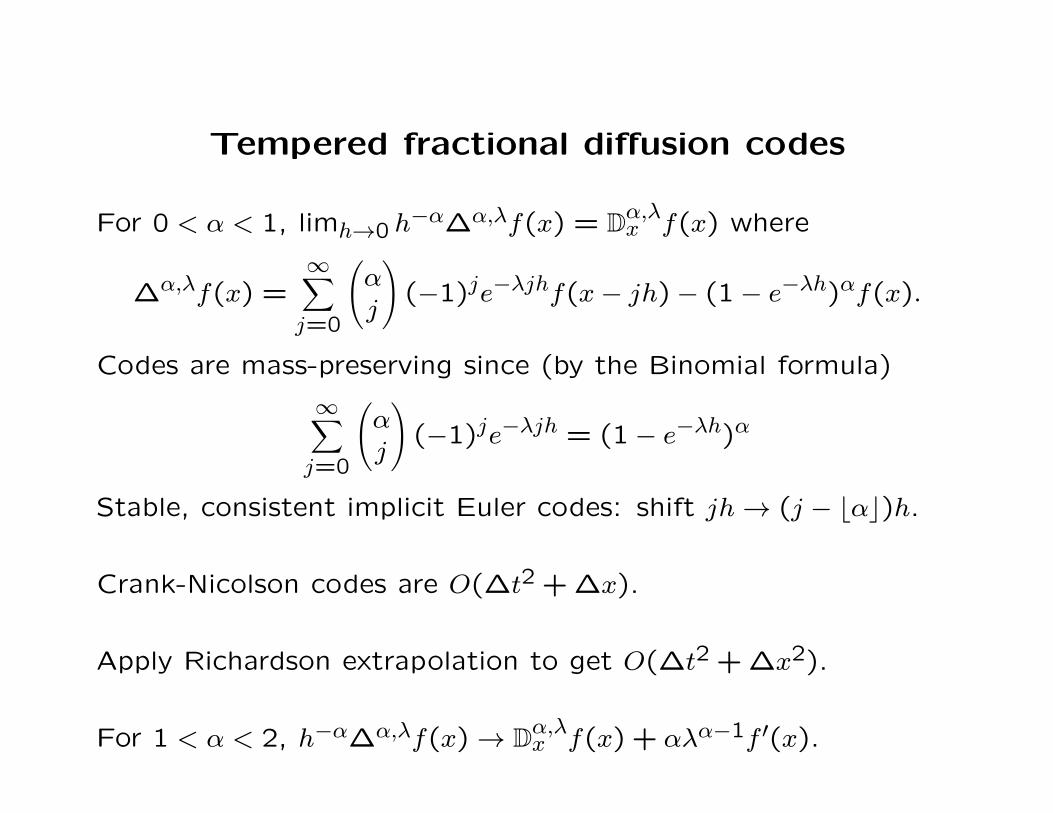
Tempered fractional diffusion codes

For 0 < α < 1, limh→0 h−α∆α,λf(x) = D

α,λx f(x) where

∆α,λf(x) =∞∑

j=0

(

αj

)

(−1)je−λjhf(x− jh)− (1− e−λh)αf(x).

Codes are mass-preserving since (by the Binomial formula)

∞∑

j=0

(

αj

)

(−1)je−λjh = (1− e−λh)α

Stable, consistent implicit Euler codes: shift jh→ (j − ⌊α⌋)h.

Crank-Nicolson codes are O(∆t2 +∆x).

Apply Richardson extrapolation to get O(∆t2 +∆x2).

For 1 < α < 2, h−α∆α,λf(x) → Dα,λx f(x) + αλα−1f ′(x).

Numerical example

Exact solution u(x, t) = xβe−λx−t/Γ(1+ β) and Crank-Nicolson

solution (extrapolated) to

∂tp(x, t) = c(x)Dα,λx p(x, t) + r(x, t)

on 0 < x < 1 with α = 1,6, λ = 2, β = 2.8, p(x,0) = xβe−λx/Γ(β+1),

p(0, t) = 0, p(1, t) = e−λ−t/Γ(β+1), c(x) = xαΓ(1+ β − α)/Γ(β+1),

and r(x, t) = r1(x, t)e−λx−tΓ(1+ β − α)/Γ(β+1) where

r1(x, t) =(1− α)λαxα+β

Γ(β+1)+αβλα−1xα+β−1

Γ(β)−

2xβ

Γ(1+ β − α).

∆t ∆x CN Max Error Rate CNX Max Error Rate

1/10 1/50 7.7738× 10−5 – 2.8514× 10−6 –

1/20 1/100 3.8353× 10−5 2.03 7.2120× 10−7 3.95

1/40 1/200 1.9055× 10−5 2.01 1.8157× 10−7 3.97

1/80 1/400 9.4976× 10−6 2.01 4.5555× 10−8 3.99

Fractional derivatives: Integral forms

In the simplest case 0 < α < 1 the generator form is

Dαxf(x) =

α

Γ(1− α)

∫ ∞

0

(

f(x)− f(x− y))

y−α−1dy.

Check: Since f(x− y) has FT e−ikyf(k), then the RHS has FT

α

Γ(1− α)

∫ ∞

0

(

1− e−iky)

f(k)y−α−1dy.

For λ > 0 it is not hard to compute [Prop. 3.10 in MS 2012]

α

Γ(1− α)

∫ ∞

0

(

1− e−(λ+ik)y)

y−α−1dy = (λ+ ik)α

and then (let λ→ 0) Dαxf(x) has FT (ik)αf(k). For 1 < α < 2

Dαxf(x) =

α(α− 1)

Γ(2− α)

∫ ∞

0

(

f(x− y)− f(x) + yf ′(x))

y−α−1dy

and again the RHS has FT (ik)αf(k).

Tempered fractional derivatives

In the simplest case 0 < α < 1 the generator form is

Dα,λx f(x) =

α

Γ(1− α)

∫ ∞

0

(

f(x)− f(x− y))

e−λyy−α−1dy.

Check: The integral on the RHS has Fourier transform

α

Γ(1− α)

∫ ∞

0

(

1− e−iky)

f(k)e−λyy−α−1dy

=α

Γ(1− α)

∫ ∞

0

(

(1− e−(λ+ik)y)− (1− e−λy))

f(k)y−α−1dy

which reduces to [(λ+ ik)α − λα]f(k).

For 1 < α < 2 we have

Dα,λx f(x) =

α(α− 1)

Γ(2− α)

∫ ∞

0

(

f(x− y)− f(x) + yf ′(x))

e−λyy−α−1dy

and the RHS has FT [(λ+ ik)α − λα − ikαλα−1]f(k).

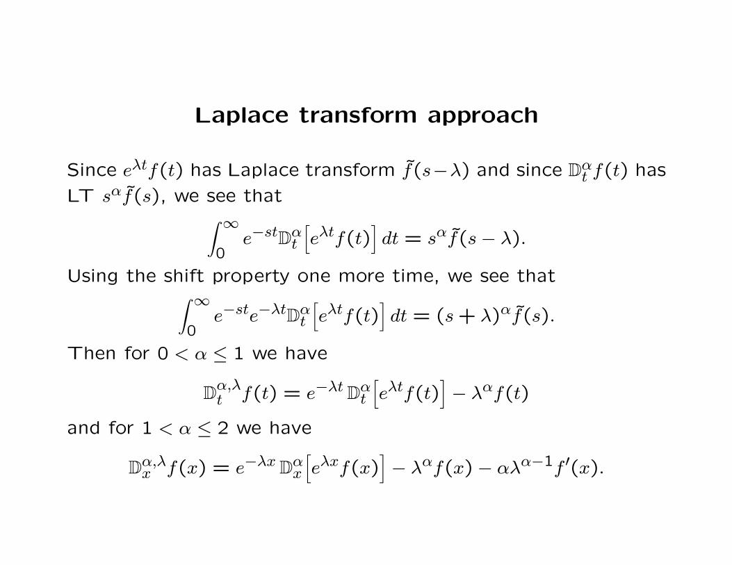
Laplace transform approach

Since eλtf(t) has Laplace transform f(s−λ) and since Dαt f(t) has

LT sαf(s), we see that∫ ∞

0e−stDαt

[

eλtf(t)]

dt = sαf(s− λ).

Using the shift property one more time, we see that∫ ∞

0e−ste−λtDαt

[

eλtf(t)]

dt = (s+ λ)αf(s).

Then for 0 < α ≤ 1 we have

Dα,λt f(t) = e−λtDαt

[

eλtf(t)]

− λαf(t)

and for 1 < α ≤ 2 we have

Dα,λx f(x) = e−λxDαx

[

eλxf(x)]

− λαf(x)− αλα−1f ′(x).

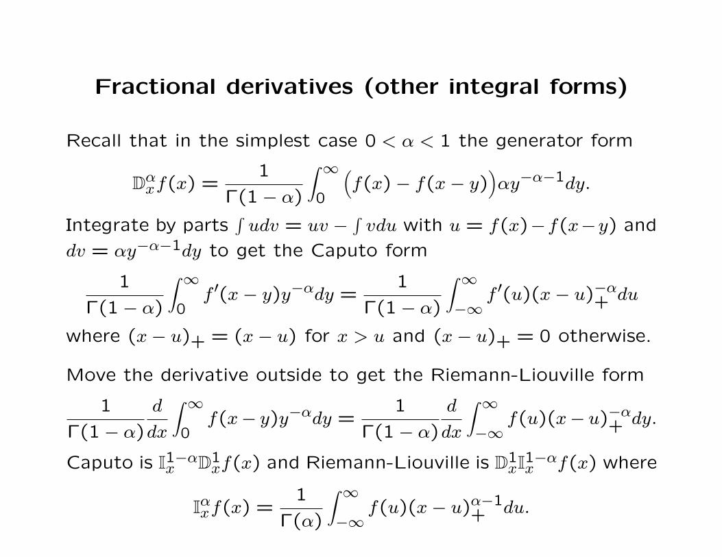
Fractional derivatives (other integral forms)

Recall that in the simplest case 0 < α < 1 the generator form

Dαxf(x) =

1

Γ(1− α)

∫ ∞

0

(

f(x)− f(x− y))

αy−α−1dy.

Integrate by parts∫

udv = uv −∫

vdu with u = f(x)−f(x−y) and

dv = αy−α−1dy to get the Caputo form

1

Γ(1− α)

∫ ∞

0f ′(x− y)y−αdy =

1

Γ(1− α)

∫ ∞

−∞f ′(u)(x− u)−α+ du

where (x− u)+ = (x− u) for x > u and (x− u)+ = 0 otherwise.

Move the derivative outside to get the Riemann-Liouville form

1

Γ(1− α)

d

dx

∫ ∞

0f(x− y)y−αdy =

1

Γ(1− α)

d

dx

∫ ∞

−∞f(u)(x− u)−α+ dy.

Caputo is I1−αx D

1xf(x) and Riemann-Liouville is D

1xI

1−αx f(x) where

Iαxf(x) =

1

Γ(α)

∫ ∞

−∞f(u)(x− u)α−1

+ du.

Fractional Brownian motion

Given Zn iid with mean zero and finite variance, the time series

Xt = ∆αZn =∞∑

j=0

(

αj

)

(−1)jZt−j

is long range dependent: E(XtXt+j) ≈ |j|2H−2 with H = 1/2−α.

Then n−H(X1+ · · ·+X[nt]) ⇒ BH(t) fractional Brownian motion.

Here BH(t) = ∂αt B(t)−∂αt B(0) where B(t) is a Brownian motion:

BH(t) =1

Γ(1− α)

∫ +∞

−∞

[

(t− u)−α+ − (0− u)−α+

]

B(du)

with B(du) = B′(u)du in the distributional sense (Caputo).

Hence FBM is the fractional integral of the white noise B(du).

Tempered fractional Brownian motion

Tempered fractional Brownian motion with −1/2 < α < 1/2:

Bα,λ(t) =∫ +∞

−∞

[

e−λ(t−u)+(t− u)−α+ − e−λ(0−u)+(0− u)−α+

]

B(du).

TFBM is the tempered fractional integral of white noise B(du):

Iα,λt f(t) =

1

Γ(α)

∫ ∞

−∞f(u)e−λ(t−u)+(t− u)α−1

+ du.

Tempered fractional Gaussian noise: Xt = Bα,λ(t)−Bα,λ(t− 1).

Semi-long range dependence: E(XtXt+j) ≈ |j|2H−2 for j small to

moderate, then E(XtXt+j) ≈ |j|−2 as j → ∞, where H = 1/2−α.

For any Zn iid with mean zero and finite variance, the time series

Xt = ∆α,λZn also exhibits semi-long range dependence.

FBM and tempered FBM

FBM (thin line) and TFBM (thick line) with same B(du) for

H = 0.3, λ = 0.03 (left) and H = 0.7, λ = 0.01 (right).

0 100 200 300 400 500

−5

05

10

t

X(t

)

0 100 200 300 400 500

−20

010

20t

X(t

)

Sample paths are Holder continuous of order H.

Scaling: BH(ct)d= cHBH(t) and Bα,λ(ct)

d= cHBα,cλ(t) .

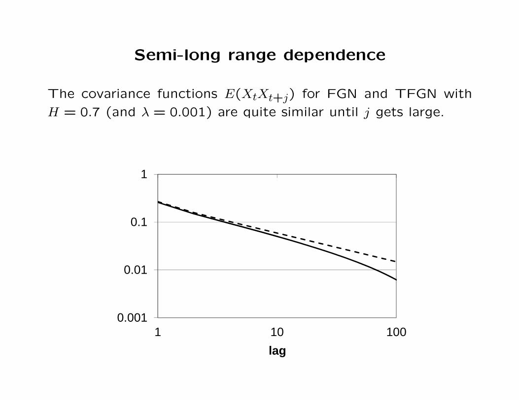
Semi-long range dependence

The covariance functions E(XtXt+j) for FGN and TFGN with

H = 0.7 (and λ = 0.001) are quite similar until j gets large.

0.001

0.01

0.1

1

1 10 100

lag

Spectral density

FGN spectral density blows up at low frequencies for H > 1/2:

fH(ω) =1

2π

∞∑

j=−∞

eiωjE(XtXt+j) ≈ |ω|1−2H as ω → 0.

For TFGN with λ ≈ 0 we get a similar result

fα,λ(ω) ≈ω2

[λ2 + ω2]H+1/2

as ω → 0.

Hence fα,λ(ω) ≈ |ω|1−2H for moderate frequencies, but remains

bounded for very low frequencies (Davenport spectrum).

Spectral density comparison

Spectral density for FGN and TFGN with H = 0.7, λ = 0.06.

0

0.05

0.1

0.15

0.2

0.25

0.3

0 0.5 1 1.5 2

frequency

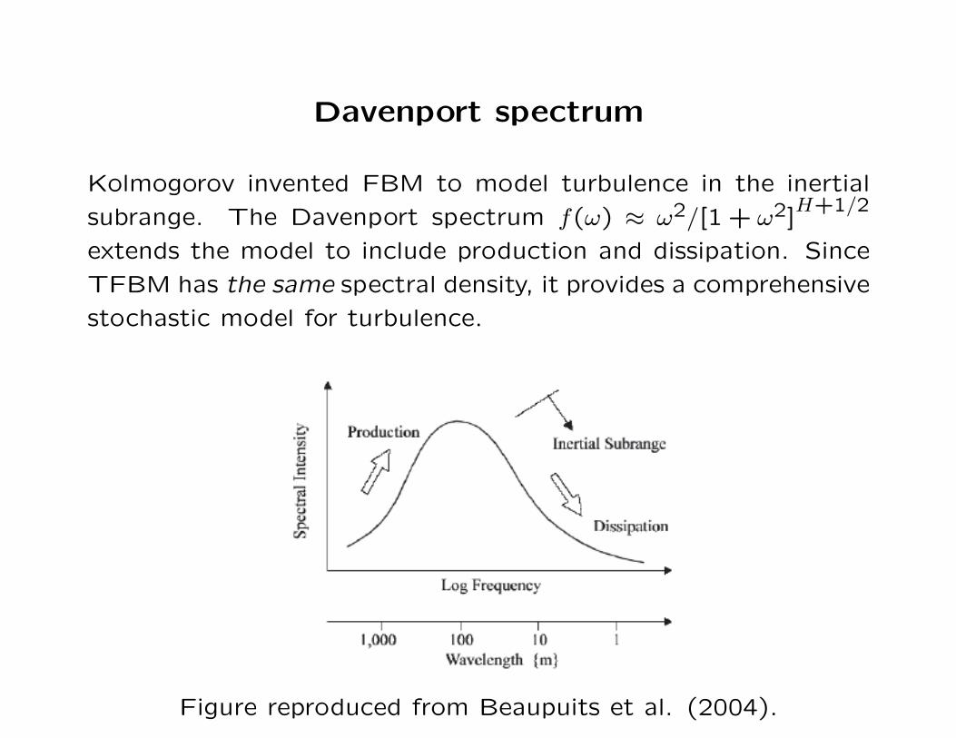
Davenport spectrum

Kolmogorov invented FBM to model turbulence in the inertial

subrange. The Davenport spectrum f(ω) ≈ ω2/[1 + ω2]H+1/2

extends the model to include production and dissipation. Since

TFBM has the same spectral density, it provides a comprehensive

stochastic model for turbulence.

Figure reproduced from Beaupuits et al. (2004).

Davenport spectrum for wind gusts

Spectral density of wind gustiness from Davenport (1961). TFBM

provides a stochastic model for the Davenport spectrum.

Wind power study

Spectral density of wind speed at the Chajnantor radio telescope

site in Chile.

Summary

• Tempered power laws

• Tempered fractional derivatives

• Numerical methods

• Tempered fractional Brownian motion

• Davenport model for wind speed

References1. I.B. Aban, M.M. Meerschaert, and A.K. Panorska (2006) Parameter Estimation for the

Truncated Pareto Distribution. Journal of the American Statistical Association: Theory

and Methods. 101(473), 270–277.

2. P. Abry, P. Goncalves and P. Flandrin (1995) Wavelets, spectrum analysis and 1/fprocesses. In Wavelets and statistics, 15–29. Springer New York.

3. B. Baeumer and M.M. Meerschaert (2010) Tempered stable Levy motion and transientsuper-diffusion. Journal of Computational and Applied Mathematics 233, 2438–2448.

4. J. P. Perez Beaupuits, A. Otarola, F. T. Rantakyro, R. C. Rivera, S. J. E. Radford,and L.-A. Nyman (2004) Analysis of wind data gathered at Chajnantor. ALMA Memo

497.

5. A. Cartea and D. del Castillo-Negrete (2007) Fluid limit of the continuous-time randomwalk with general Levy jump distribution functions. Phys. Rev. E 76, 041105.

6. A. Chakrabarty and M. M. Meerschaert (2011) Tempered stable laws as random walklimits. Statistics and Probability Letters 81(8), 989–997.

7. A. V. Chechkin, V. Yu. Gonchar, J. Klafter and R. Metzler (2005) Natural cutoff inLevy flights caused by dissipative nonlinearity. Phys. Rev. E 72, 010101.

8. S. Cohen and J. Rosinski (2007) Gaussian approximation of multivariate Levy processeswith applications to simulation of tempered stable processes, Bernoulli 13, 195-210.

9. A. G. Davenport (1961) The spectrum of horizontal gustiness near the ground in highwinds. Quarterly Journal of the Royal Meteorological Society 87, 194–211.

10. P. Flandrin (1989) On the spectrum of fractional Brownian motions. IEEE Trans. onInfo. Theory IT-35, 197199.

11. R. N. Mantegna and H. E. Stanley (1994) Stochastic process with ultraslow convergenceto a Gaussian: The truncated Levy flight. Phys. Rev. Lett. 73, 2946–2949.

12. M.M. Meerschaert and H.P. Scheffler (2001) Limit Theorems for Sums of Independent

Random Vectors: Heavy Tails in Theory and Practice. Wiley Interscience, New York.

13. M.M. Meerschaert and H.P. Scheffler (2004) Limit theorems for continuous-time ran-dom walks with infinite mean waiting times. J. Appl. Probab. 41(3), 623–638.

14. Meerschaert, M.M., Scheffler, H.P. (2008) Triangular array limits for continuous timerandom walks. Stoch. Proc. Appl. 118(9), 1606-1633.

15. Meerschaert, M.M., Y. Zhang and B. Baeumer (2008) Tempered anomalous diffusionin heterogeneous systems. Geophys. Res. Lett. 35, L17403.

16. M.M. Meerschaert and A. Sikorskii (2012) Stochastic Models For Fractional Calculus.De Gruyter, Berlin/Boston.

17. Meerschaert, M.M., P. Roy and Q. Shao (2012) Parameter estimation for temperedpower law distributions. Communications in Statistics Theory and Methods 41(10),1839–1856.

18. M.M. Meerschaert (2013) Mathematical Modeling. 4th Edition, Academic Press, Boston.

19. M.M. Meerschaert and F. Sabzikar (2013) Tempered fractional Brownian motion.Preprint at www.stt.msu.edu/users/mcubed/TFBM5.pdf

20. Rosinski, J. (2007), Tempering stable processes. Stoch. Proc. Appl. 117, 677–707.

21. C. Tadjeran, M.M. Meerschaert, H.P. Scheffler (2006) A second order accurate nu-merical approximation for the fractional diffusion equation. Journal of Computational

Physics 213(1), 205–213.

Simulating tempered stable laws

Simulation codes for stable random variates are widely available.

If X > 0 has stable density density f(x), TS density is

fλ(x) =e−λxf(x)

∫ ∞

0e−λuf(u) du

Take Y ∼ exp(λ) independent of X, (Xi, Yi) IID with (X,Y ).

Let N = min{n : Xn ≤ Yn}. Then XN ∼ fλ(x).

Proof: Compute P (XN ≤ x) = P (X ≤ x|X ≤ Y ) by conditioning,

then take d/dx to verify.

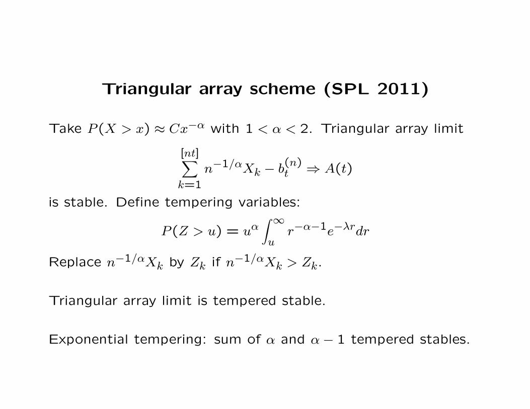
Triangular array scheme (SPL 2011)

Take P (X > x) ≈ Cx−α with 1 < α < 2. Triangular array limit

[nt]∑

k=1

n−1/αXk − b(n)t ⇒ A(t)

is stable. Define tempering variables:

P (Z > u) = uα∫ ∞

ur−α−1e−λrdr

Replace n−1/αXk by Zk if n−1/αXk > Zk.

Triangular array limit is tempered stable.

Exponential tempering: sum of α and α− 1 tempered stables.

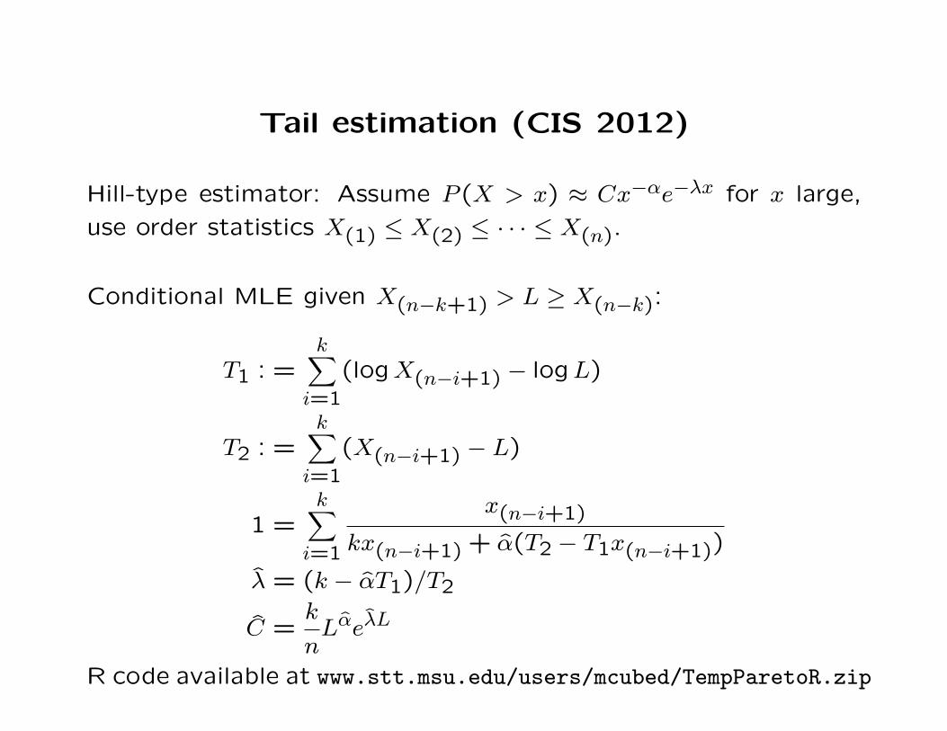
Tail estimation (CIS 2012)

Hill-type estimator: Assume P (X > x) ≈ Cx−αe−λx for x large,

use order statistics X(1) ≤ X(2) ≤ · · · ≤ X(n).

Conditional MLE given X(n−k+1) > L ≥ X(n−k):

T1 : =k∑

i=1

(logX(n−i+1) − logL)

T2 : =k∑

i=1

(X(n−i+1) − L)

1 =k∑

i=1

x(n−i+1)

kx(n−i+1) + α(T2 − T1x(n−i+1))

λ = (k − αT1)/T2

C =k

nLαeλL

R code available at www.stt.msu.edu/users/mcubed/TempParetoR.zip

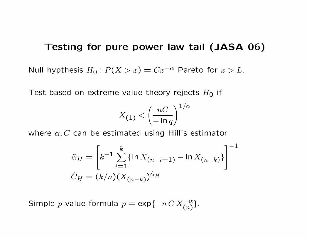
Testing for pure power law tail (JASA 06)

Null hypthesis H0 : P (X > x) = Cx−α Pareto for x > L.

Test based on extreme value theory rejects H0 if

X(1) <

(

nC

− ln q

)1/α

where α,C can be estimated using Hill’s estimator

αH =

k−1k∑

i=1

{lnX(n−i+1) − lnX(n−k)}

−1

CH = (k/n)(X(n−k))αH

Simple p-value formula p = exp{−nC X−α(n)

}.