Embed Size (px)
Citation preview
The Elusive Effects of Trade on Growth: Export Diversity and Economic Take-Off*
Theo S. Eicher University of Washington
David J. Kuenzel
Wesleyan University
Version 2.4
Abstract
The hallmark of the voluminous growth determinants literature is the absence of a clear-cut effect of trade on growth. Numerous candidate regressors have been motivated by alternative theories and tested by a multitude of empirical studies, but not one trade regressor has been robustly related to growth. In this paper, we leverage Melitz’ (2003) insights regarding sectoral export dynamics and Feenstra and Kee’s (2008) approach to productivity and sectoral export diversity to propose a structured approach to trade and growth determinants. Instead of relying on aggregate trade measures as previous studies, we examine the diversity of sectoral exports and the development of broad-based comparative advantage as a potential growth determinant. Controlling for model uncertainty and endogeneity, we find that export diversity serves as a crucial growth determinant for low income countries, an effect that weakens with the level of development.
JEL codes: F14, F43, O47 Keywords: Export Diversity, Trade and Growth Determinants, Bayesian Model Averaging
___________________________
* Contact information: Eicher: Department of Economics, 305 Savery Hall, University of Washington, E-mail: [email protected]. Kuenzel: Department of Economics, PAC 123, Wesleyan University, E-mail: [email protected]. We thank Chih Ming Tan, Andros Kourtellos and Chris Papageorgiou for sharing their data and for extensive discussions. We also wish to thank attendees of the Spring 2014 Midwest International Trade Meetings, the 2014 Workshop in Macroeconomic Research at Liberal Arts Colleges, and DEGIT XIX at Vanderbilt University, as well as seminar participants at Harvard Kennedy School for their helpful comments and suggestions. This work benefited from the financial support of the U.K.'s Department for International Development (DFID).
1
I. Introduction
The elusive effects of trade are a fundamental puzzle in the growth determinants literature.
Numerous theories link trade to economic growth, but exhaustive analyses of growth
determinants have not produced robust trade effects.1 Endogeneity bias compounds the issue
since feedback effects from growth to trade are commonly ignored in studies that examine a
wide range of growth determinants.2 Complicating matters further are the multitude of trade
channels and their positive or negative effects on growth that different trade theories suggest.
When competing theories propose alternative candidate regressors and/or opposing effects, the
associated model uncertainty may artificially inflate t-statistics (see Raftery, 1995, and Raftery
and Zheng, 2003).
In this paper, we extend the empirical trade-and-growth literature in two dimensions.
First, we identify trade effects on growth by focusing not on the volume but the composition of
trade. While previous growth determinant approaches use aggregate trade measures, we examine
trade-driven growth through sectoral export diversification. We do not rely on aggregate tariff
levels or aggregate trade volumes, but instead examine variations in the breadth of countries’
comparative advantages across sectors as a potential growth determinant. Second, we
simultaneously address model uncertainty and endogeneity to produce consistent test statistics
and reduce the associated endogeneity and omitted variable bias.
Levine and Renelt (1992) first included a number of trade measures in their seminal study
of growth determinants and reported that no trade measure is robustly linked to growth. “Primary
Export Shares”, “Openness” (import+export share of GDP) and/or “Years Open”3 have since
become standard candidate growth determinants, although it is well known that neither variable
is robust. Sala-i-Martin (1997) subsequently used Levine and Renelt’s “Openness” measure and
added “Primary Export Shares” and “Years Open”. Only after lowering Renelt and Levine’s
extreme bound effect-thresholds, he found “Years Open” and “Primary Export Shares” to be
1 Rodriguez and Rodrik (2001) provide a skeptics’ guide to the related literature of reduced-form trade-policy-and-growth empirics which includes trade measures but only a fraction of potentially relevant growth determinants. The authors side with Edwards’ (1993) previous trade-and-growth survey assessment that these studies “have been plagued by empirical and conceptual shortcomings. The theoretical frameworks used have been increasingly simplistic, failing to address important questions such as the exact mechanism through which export expansion affects GDP growth.” 2 The exceptions are Barro (2003) and Durlauf et al. (2008). 3 The fraction of years in the period 1950-1990 for which Sachs and Warner (1995) rate a country “open to trade”.

2
robust, but his approach was called into question because it highlighted the arbitrary width of the
extreme bounds. Sala-i-Martin’s analysis has since been reexamined in a multitude of studies
using Bayesian Model Averaging (BMA) where effect-thresholds are theory-specified. Using the
original (and/or updated) Sala-i-Martin data, in cross sections and/or panels, with different
parameter and/or model priors, not a single paper identifies any one of the above trade measures
as exerting a decisive effect on growth.4 In the most recent and the most extensive analysis of
trade, growth and model uncertainty (without controlling for endogeneity, however), Eris and
Ulasan (2013) examine “Openness”, “Real Openness”, “Years Open”, “Tariff Rates”,
“NonTariff Barriers” and “Black Market Premiums” to find “no evidence that trade openness is
directly and robustly correlated with economic growth in the long run.”
To better understand how trade affects growth, we move away from aggregate trade
measures and focus on sectoral export diversity. Our fine-grained approach highlights that it is
the evolution of export sectors along the development path that affects economic growth.5 To
measure export diversity, we use the extensive margin measure introduced by Hummels and
Klenow (2005), which is based on earlier work by Feenstra (1994).6 The Hummels-Klenow
measure has been employed extensively in studies of export diversity and income patterns –
although its connection to economic growth has not been explored to date. The descriptive
literature examining export diversity and income patterns finds conflicting results. For advanced
countries, income was found to be correlated with increasing or constant export diversification
(Proudman and Redding, 2000, and Funke and Ruhwedel, 2001). Studies utilizing global panels
find that exports first diversify and then re-concentrate with income (Cadot et al., 2011, and
Papageorgiou and Spatafora, 2012), or that diversity is rising throughout, but with decreasing
intensity (Brasili et al., 2000, De Benedictis et al., 2009, Parteka, 2010, and Besedes and Prusa,
2011). The only salient and uncontroversial feature of this literature is then that diversification
levels differ distinctly by development stages. That is, the relationship between diversity and
4 See Fernández at al. (2001), Brock and Durlauf (2001), Sala-i-Martin et al. (2004), Durlauf et al. (2008), Ciccone and Jarocinski (2010) and Eicher et al. (2011). Note that BMA results have better predictive performance and a lower Mean Squared Error than any single regression model (Raftery and Zheng, 2003). 5 We discuss the various theories that give rise to such a hypothesis in the following section. 6 Our empirical results are robust to using other export diversity measures commonly employed in the literature, such as Herfindahl, Gini and Theil indices. Detailed results are provided below in the robustness section.

3
income is positive for low income countries while the correlation for high income countries is
somewhat uncertain.7
Our approach to identifying an effect of export diversity on growth builds on Durlauf et
al.’s (2008) seminal BMA panel study of growth determinants, which is itself based on the
methodology and dataset of Barro (2003). We extend the time dimension of the Durlauf et al.
panel and introduce export diversity as a potential growth determinant. In addition, we utilize a
methodology that fully accounts for model uncertainty in the presence of endogeneity, since
Durlauf et al. examined model uncertainty in the second stage only (Barro, 2003, does not
consider model uncertainty or endogeneity).
Our findings confirm the Durlauf et al. results that aggregate trade volumes are not a
robust growth determinant in a panel of countries. Once we introduce export diversity, however,
we find that the breadth of a country’s exports is a crucial determinant of economic growth for
low income economies. The effect is associated with a high posterior probability and it is also
economically important: a one standard deviation increase in export diversity for low income
countries is shown to increase their average annual growth rate by one percentage point.
Interestingly, there is also evidence that the effect of export diversity on low income countries is
amplified by reliance on primary exports. The greater the primary export reliance of a low
income country, the larger is the growth impact of diversification.
Aside from export diversity, the growth determinants suggested by our approach are
those central to all previous studies: “InitialGDP”, “PopulationGrowth” and “Investment” reflect
neoclassical growth models; “GovernanceQuality” and “GovernmentExpenditures” represent
new growth theories; and there is also support for theories that link religion to growth as
indicated by the importance of the “JewishFraction” of the population. In addition, we show
explicitly that a country’s terms-of-trade, real exchange rate, trade agreement memberships,
openness, FDI flows and GDP volatility do not drive the effect of export diversity on growth.
7 The descriptive literature also developed stylized facts that relate export diversity to aggregate trade growth. Hummels and Klenow (2005) show that larger (in terms of GDP) and richer countries (in terms of GDP per capita) have greater trade volumes and more diversified exports. Brenton and Newfarmer (2007) document that increased export diversity accounts for 20 percent of trade growth in developing nations, while Kehoe and Ruhl (2013) show that it explains 10 percent of trade growth in advanced countries. Below we take this literature one step further and examine the effects of diversity on economic growth.

4
Previously, Feenstra and Kee (2008) examined the relationship between productivity and
export diversity in a Melitz (2003) type model of heterogeneous firms. In Feenstra and Kee’s
approach, greater export diversity causes increases in a country’s average productivity. In their
empirical specification, they then examine the link between income levels and export diversity
using standard gravity controls but not allowing for any other alternative income determinants
(e.g., investment, education, etc.). Our approach differs substantially as we ask whether export
diversification drives income growth after having controlled for 28 competing growth
determinants. We consider a host of alternative theories, ranging from governance quality,
investment, religion, inflation, life expectancy and education to geographic factors. In addition,
we apply an appropriate growth framework that features “InitialGDP” and employ an
econometric methodology that is designed to juxtapose alternative growth theories (IVBMA) in
the presence of endogeneity. Moreover, Feenstra and Kee restrict their analysis to the exports of
48 countries to the United States from 1980-2000 while we examine the diversity of global
exports for 84 countries from 1965-2009. Finally, we investigate not only the extensive but also
the intensive margin of exports in our robustness section.
The remainder of the paper is organized as follows. Section II sketches the various links
between trade, diversity and growth suggested in the literature and highlights the importance of
model uncertainty in this context. The section also discusses our preferred measure of export
diversity and our empirical specification. Section III provides an overview of the IVBMA
methodology. Section IV describes the structure of the panel of countries used in our empirical
analysis and also introduces alternative export diversity measures considered in the literature.
Section V presents a discussion of the empirical results. Section VI considers a range of
robustness checks and section VII concludes.
II. Trade, Export Diversity and Growth Determinants
II.1 Theory and Empirics
To appreciate the dichotomy between the absence of significant trade effects in growth
regressions and the number of theories that relate trade to growth, we briefly summarize the trade
and growth effects and their associated candidate regressors that have been suggested by
different strands of trade theories. Neoclassical trade theories focus on static comparative

5
advantage (productivity and endowment differences) and aggregate trade volumes (see, e.g.,
Bernhofen, 2011). In order to control for this channel, we include in our empirical model the
standard trade volume measure (“Openness”), which we filter for population and country size as
in Barro (2003) and Durlauf et al. (2008). In the absence of cross-country productivity data for
our sample, we also include “FDIInFlow” and “FDIOutFlow” in the robustness section VI as
proxies for productivity.
Strategic Trade models rely instead on monopolistic competition where export product
differentiation is crucially affected by market size (e.g., Dixit and Norman, 1980, and Krugman,
1980). In this literature, scale economies allow larger markets to produce and export a greater
quality/variety of goods. Hence we include below country size (“lLand”) and population
(“lPop”) as determinants for diversity. Country size has also previously been linked to export
diversity in empirical studies (e.g. Hummels and Klenow, 2005). Strategic Trade models are thus
the first to provide a clear justification for focusing on sectoral export diversity instead of
aggregate measures of trade and productivity.
New Trade theories rely on dynamic sectoral reallocation and growth in quality and/or
variety via sectoral spillovers in innovation, learning, or knowledge capital investment (Young,
1991, Rivera-Batiz and Romer, 1991, and Grossman and Helpman, 1991). These theories link
export diversity to growth accelerations via the extensive margin, since new sectors generate
additional learning, spillovers, and incentives to invent additional varieties or better qualities that
increase real incomes in perpetuity. Here it is important to note that the predicted effect of
diversity on growth may be neither linear nor monotone, depending on the extent of cross-
country knowledge spillovers. Laggard countries may well experience growth reductions when
trade shifts production towards less dynamic sectors in terms of learning, spillover or R&D
intensive goods. Such spillovers are facilitated by a country’s level of human capital
(“Education”) which we include as control below.
The next generation of “New-New” Trade theories links export diversity to heterogeneity
in firms’ productivities (e.g., Feenstra and Kee, 2008, and Baldwin and Robert-Nicoud, 2008).
Feenstra and Kee (2008) highlight the positive link between export diversity (the share of
exporting firms), income and average sectoral productivity. If exporting firms are more
productive than only domestically active firms, a greater share of exporters (or varieties)

6
increases productivity and income in an economy. While sectoral productivity data is not
available for our global sample to implement the Feenstra and Kee’s hypothesis, we can capture
the dynamic evolution of exports by considering countries’ extensive trade margins. As in the
case of New Trade theories, heterogeneous firm trade models do not predict a uniform impact of
export diversity on growth across development stages. In particular, the positive impact of export
diversity on sectoral TFP levels is decreasing with income as long as export revenues raise
domestic GDP at a declining rate.8 This condition is more likely to hold in more developed
economies which rely less on export revenue to stimulate internal demand. In addition, Baldwin
and Robert-Nicoud (2008) show that if productivity is modeled endogenously in a heterogeneous
firm environment, the relation between trade, export diversity and growth depends on the
evolution of the cost of innovation as a country grows richer. Economic growth might slow or
accelerate depending upon the impact of trade and diversity on the marginal cost of innovation.
Alternative channels that suggest links between export diversity and economic growth are
based on primary export reliance, output volatility, or preferential trade agreements. Prebisch
(1950) and Singer (1950) highlight the detrimental effects of excessive specialization in primary
exports and deteriorating terms-of-trade on economic development. Hence we also include
primary export shares (“PrimaryX”), the terms-of-trade (“TOT”) and terms-of-trade volatility
(“TOTVolatility”) as controls in our robustness analysis below. Koren and Tenreyro (2007) find
that GDP is much more volatile in poor countries which specialize in fewer and more volatile
sectors. In a similar vein, Raddatz (2011) suggests that export diversity insures against exchange
rate variability. To account for these channels, we consider in our robustness analysis the real
effective exchange rate (“REER”), as well as measures of exchange rate volatility
(”FXVolatility”) and output volatility (“GDPVolatility”). In addition, we control for potential
effects of bilateral and multilateral preferential trade agreements (“WTO” and “PTA”). Even
though trade agreements are not part of standard growth regression frameworks, we include
variables that capture WTO and PTA membership to rule out that any diversity effects may be
driven by membership-induced tariff reductions.
Finally, note that the traditional “Openness” measure and “PrimaryX” are predicted to
simultaneously exert an impact on both export variety and the evolution of incomes. From an 8 This result emerges when differentiating relative sectoral TFP, as given by equation (32) in Feenstra and Kee (2008), with respect to domestic export diversity ( h
ixtM ) and the domestic sectoral GDP share, hits .
7
econometric perspective, it is therefore possible that any export diversity effect on growth is
amplified by either of these variables, which could be missed when not properly accounting for
potential interlinkages. We therefore also test below whether “Openness” and “PrimaryX” act as
hidden catalysts for potential export diversity effects on growth.
II.2 Measuring Export Diversity and Additional Covariates
As our discussion shows, dynamic and static trade models provide diverse trade and growth
channels that might differ in importance depending on a country’s level of development. The
importance of trade for growth is then best captured by examining sectoral export diversity, since
it allows for a disaggregation of trade flows to account for dynamic trade effects. To quantify the
effect of sectoral export expansion on growth, we use the extensive margin measure suggested
by Hummels and Klenow (2005), which has the advantage of being firmly rooted in trade
theory.9 The Hummels-Klenow measure appropriately integrates new products into price indices
(see Feenstra, 1994) which is crucial in dynamic sectoral studies. Specifically, the extensive
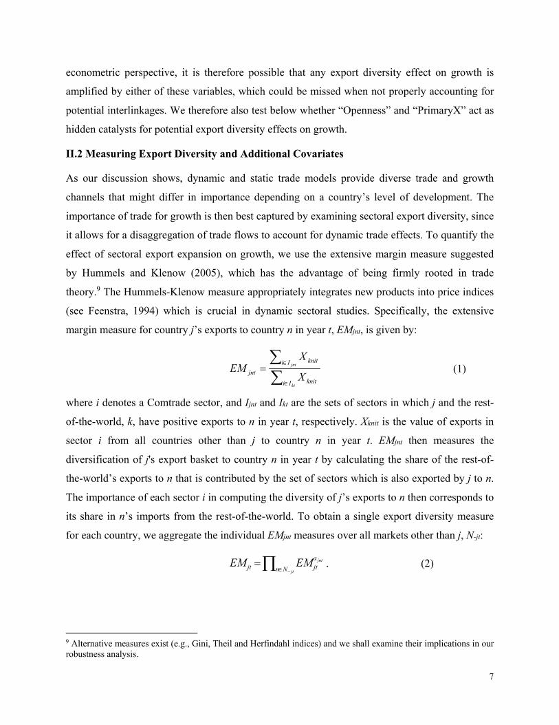
margin measure for country j’s exports to country n in year t, EMjnt, is given by:
kt
jnt
Ii knit
Ii knit
jnt X
XEM (1)
where i denotes a Comtrade sector, and Ijnt and Ikt are the sets of sectors in which j and the rest-
of-the-world, k, have positive exports to n in year t, respectively. Xknit is the value of exports in
sector i from all countries other than j to country n in year t. EMjnt then measures the
diversification of j's export basket to country n in year t by calculating the share of the rest-of-
the-world’s exports to n that is contributed by the set of sectors which is also exported by j to n.
The importance of each sector i in computing the diversity of j’s exports to n then corresponds to
its share in n’s imports from the rest-of-the-world. To obtain a single export diversity measure
for each country, we aggregate the individual EMjnt measures over all markets other than j, N-jt:
jt
jnt
Nn
ajtjt EMEM . (2)
9 Alternative measures exist (e.g., Gini, Theil and Herfindahl indices) and we shall examine their implications in our robustness analysis.

8
Following Hummels and Klenow (2005), ajnt weighs the individual diversity measures by the
logarithmic mean of country n's share in country j's and the rest-of-the-world’s year t exports.10
Identifying the effect of export diversity on economic growth is, however, complicated
by endogeneity considerations. A country’s growth rate may be a key determinant of its ability to
invest into R&D, which in turn drives the number of new product varieties that can be exported.
To address endogeneity, we instrument our export diversity measure in the spirit of Frankel and
Romer (1999) with a number of exogenous geographical features: the log of a country’s land
area, a dummy taking the value one for landlocked countries, and the log of a country’s
population.
All additional covariates and instruments used in our empirical analysis below were
obtained from Durlauf et al. (2008) and the associated data update in Henderson et al. (2012).
Durlauf et al. base the selection of their variables on Barro (2003), which was previously one of
the most comprehensive approaches to growth determinants in a panel of countries. Durlauf et al.
include proxies for seven different growth theories, including regressors suggested by I)
neoclassical growth theory (“InitialGDP”, “PopulationGrowth”, “Investment”, and “Education”).
We follow Durlauf et al. and instrument for these four variables with one-period lagged values in
the absence of available data on alternative instruments. Also included are II) proxies for
demographic change (“LifeExpectancy”, “Fertility”) and III) theories that link macroeconomic
policies to growth (“GovernmentExpeditures”, “Openness” and “Inflation”). As in Durlauf et al.,
the latter three variables are instrumented with their respective lagged values. We also consider
IV) geographical features (land area within 100km of ice-free coast – “LandNearCoastPct”,
percent tropical land area – “LandTropicsPct”) and V) theories linking institutions to growth
(“ExpropriationRisk”, “ExecutiveConstraints” and “GovernanceQuality”). In addition, we
include dummy variables for the English and French origin of a country’s legal system
(“LegalOriginsUK”, “LegalOriginsFrench”) and use lagged values of “ExpropriationRisk” as
instrument for the current value of the same variable. VI) Theories relating to religion and
growth are proxied using the shares of all major religions in a country’s population
(“EasternFraction”, “HinduFraction”, “JewishFraction”, “MuslimFraction”, “OrthodoxFraction”,
10 Formally, let λ be country n's share in country j's overall exports at time t, and Λ be the rest-of-the-world’s export share to n, then
jtNnjnta lnlnlnln .
9
“ProtestantFraction” and “OtherReligionsFraction”). As Durlauf et al., we use the respective
religious shares in 1900 as instruments. Finally, we also include regressors capturing VII)
theories that predict a detrimental effect of ethnic tensions on growth (using
“LinguisticFractionalization” and “EthnicFractionalization” indices). Exact definitions and
sources of each variable are provided in the appendix.
III. Model Uncertainty and Endogeneity
Competing growth theories and their associated candidate regressors have given rise to a sizable
literature that seeks to identify robust growth determinants. Early approaches used Leamer’s
(1978) Extreme Bound Analysis (see Levine and Renelt, 1992, and Sala-i-Martin, 1997), which
suffers from arbitrary robustness thresholds for the extreme bounds. Subsequent approaches
employ Bayesian Model Averaging, which was developed specifically to address model
uncertainty empirically (Fernandez at al., 2001, Brock and Durlauf, 2001, Sala-i-Martin et al.,
2004, Ciccone and Jarocinski, 2010, and Eicher et al., 2011). None of the above approaches
tackle endogeneity, however, since the nested nature of the Instrumental Variable (IV) estimation
poses challenges for direct model comparisons.
A number of different econometric approaches have since been designed to address
endogeneity and model uncertainty simultaneously. Durlauf et al. (2008), Cohen-Cole et al.
(2009) and Durlauf et al. (2012) consider approximations of marginal likelihoods in a framework
similar to two-stage least squares. Lenkoski et al. (2014) continue this development with an
Instrumental Variable Bayesian Model Averaging (IVBMA) methodology, which uses a
framework developed by Kleibergen and Zivot (2003) and a two-stage extension of the unit
information prior (Kass and Wasserman, 1995). A similar approach has been developed by Chen
et al. (2009). Moral-Benito (2012) considers a likelihood function for dynamic panel models,
which Moral-Benito (2012b) extends to models with weakly exogenous regressors that are
combined with BMA techniques. Koop et al. (2012) develop a Bayesian IV methodology based
on a Reversible Jump Markov Chain Monte Carlo algorithm which may, however, encounter
significant mixing difficulties. Karl and Lenkoski (2012) introduce Conditional Bayes Factors
for model comparison and resolve these mixing difficulties by using a MC3-Within-Gibbs search

10
algorithm. Below we sketch the Lenkoski et al. (2014) approach in the interest of providing
intuition on how BMA can be extended to resolve endogeneity.
The IVBMA estimator by Lenkoski et al. (2014) functions as a two-step BMA procedure
where final model weights take into account uncertainty in both stages. Traditionally,
endogeneity is addressed by applying 2SLS and certifying over-identification and instrument
restrictions in the canonical setup
x
wy ' , (3)
xzw xz'' , (4)
where y is the dependent variable, x is a set of covariates, w is the set of endogenous variables,
and z is the set of instruments. The x and x are of dimension xp , and z and z have
dimension zp . To simplify the exposition, we assume that w is univariate. Assuming that
22
22
,0
0~
N , (5)
the classical endogenous variable situation arises when 02 , causing w to violate the
regression assumption of independence of the error term, . The determination of w then leads
to inconsistent estimates of the entire coefficient vector, . 2SLS solves the consistency
problem, but relies on the existence of a set of instrumental variables (IV), z, which are
independent of y, given w and the vector of covariates, x. The IV-based estimates,
ywwwIV '' 1 , obtained using the fitted values from the first stage, w , are consistent if the
conditional independence assumptions are valid.
Intuitively, IVBMA combines the IV and BMA methodologies. It processes the data
much like a two-stage least square estimator while also addressing model uncertainty in both
stages. The first stage is a straight BMA application to identify effective instruments. Let be a
quantity of interest and let the set of potential models in the first stage, M~
, be comprised of
MMi
~~ individual models. The posterior distribution of conditional on the data, D, is then

11
given by the weighted average of the predictive distribution under each model, using as weights
the models’ corresponding posterior probabilities:
MM iii
DMprDMprDpr ~~ |~
,~
|| , (6)
where DMpr i ,~
| is the predictive distribution and DMpr i |~
is the posterior model
probability of model iM~
. The posterior model probability, i~, for each model in the first stage is
given by
iiii MprMDprDMpr~~
||~~ , (7)
where
iiiiii dMprMDprMDpr ~|
~,|
~| (8)
is the integrated likelihood of model iM~
with model parameters i . The prior densities for
parameters and models are given by ii Mpr~
| and iMpr~
, respectively. The posterior mean of
the model parameters in stage 1 is then
iMM iBMAi
~ˆˆ~~
, (9)
which is given by the average of the parameter estimates from each model, i , weighted by their
respective posterior model probabilities. Similarly, the posterior variance can be calculated as
MM BMAiiMM iiBMAii
~~2
~~22 ˆˆ~ˆ~ˆ . (10)
The variance has a clear interpretation that highlights how model uncertainty is accounted for by
standard errors of the BMA methodology. The first term in (10) is the weighted variance for each
model, DMVar iii ,~
|ˆˆ 2 , summed over all relevant models, and the second term indicates how
stable the estimates are across models. The more the estimates differ across models, the greater is
the posterior variance.
The posterior distribution for a parameter is a mixture of a regular posterior distribution
and a point mass at zero, which represents the probability that the parameter equals zero. The
12
sum of the posterior probabilities of the models that contain the variable is called the posterior
inclusion probability (PIP) and can then be taken as a measure of the importance of a variable:
Ai MM iBMA Dpr ~~~|0ˆ . (11)
where AM~
is the set of models in the first stage in which parameter is not constrained to zero.
IVBMA is then a nested approach that first determines the posterior model probabilities
in the first stage according to the BMA methodology, and then uses the predicted values from
each model, iw , to derive the second stage model posterior model probabilities, ij w , and
estimates, ij w . The set of models in the second stage is denoted by M, which consists of all
second stage models MM j .
The posterior means for the second stage can then be derived to be
MM MM ijijiIVBMAi j
ww~~ˆ~~
ˆ , (12)
which implies that the IVBMA estimate is formed as the average of the IV estimates obtained
using the fitted values from each first stage model, iM~
, weighted by both the respective quality
of the first and second stage specifications.
The posterior variance of IVBMA~ˆ reflects again the average variation of the estimated
parameters in all models, and how estimates differ across models in both the first and second
stages, just as captured by 2ˆBMA in the canonical BMA setup in (10). However, IVBMA also
takes into account the model weights derived in the first stage so that the posterior variance is
again weighted by the quality of its instrumenting models:
2
~~ ,~~22
~ˆ][ˆ~][ˆ~~
ˆ
MM IVBMAiBMAiiMM iBMAiIVBMAii
ww . (13)
The posterior variance of IVBMA estimates can be again decomposed into two parts. The first
term in (13) is the average of the second stage BMA variances associated with a particular first
stage model iM~
. The second term indicates the stability of the individual BMA estimates
obtained with particular first stage models relative to the IVBMA estimate. Therefore, results

13
generated by underperforming instrument models are deemphasized, while those based on strong
instrument models receive relatively high posterior weights.
A similar interpretation holds for the IVBMA posterior inclusion probabilities:
MM MM ijiIVBMAi Aj
wDpr ~~~)|0ˆ(][ (14)
where MA indicates the subset of second stage models for which the coefficient β is not
constrained to zero. Standard rules of thumb for interpreting IVBMA have been provided by Kass
and Raftery (1995). They establish the following effect-thresholds: < 50% evidence against the
effect, 50-75% weak evidence for the effect, 75-95% positive evidence, 95-99% strong evidence,
and > 99% decisive evidence.
IV. Data
The dataset is an unbalanced panel of 84 countries from 1965 to 2009. Using 5-year periods, the
dataset comprises 589 country-period observations. To extend the datasets of Durlauf et al.
(2008) and Henderson et al. (2012), we use government expenditures as share of GDP instead of
government expenditures net of education and military expenditures. In addition, the Durlauf et
al. “Cheque” data on legal procedures required to collect a bounced check is only available for a
limited set of countries from the World Bank Doing-Business Indicators. Djankov et al. (2003)
and La Porta et al. (2008) document the strong empirical relationship between legal origin and
current legal procedures and standards, hence we substitute “LegalOrigins” (French and English)
for the “Cheque” variable in our regressions.
Since our focus is on the relationship between diversity and growth, we exclude resource-
rich economies from our analysis (specifically countries that generate more than 20 percent of
their GDP from resource rents as reported by the World Development Indicators). Resource-rich
countries represent sizable outliers with unusually low export diversity and uncommonly high
income levels. Neither the extension of the dataset beyond the original Durlauf et al. data nor the
exclusion of resource rich countries affects our results qualitatively.
The dependent variable in our analysis is average per capita GDP growth over each 5-
year period. Growth rates were calculated using data on per capita incomes from the Penn World
14
Tables versions 6.2 (1965-2004) and 7.1 (2005-2009). To control for spatial and time effects on
growth, we also include period and regional dummies: “SubSaharanAfrica”, “EastAsia” and
“LatinAmerica” (including the Caribbean). To construct the Hummels and Klenow (2005)
extensive margin measure of export diversification, we use trade data from Feenstra et al. (2005)
(4-digit SITC 1965-1989) and from the UN Comtrade database (6-digit HS 1990-2009).11
Sectoral exports for both classifications were compiled using mirror import data.
In our robustness section we also provide estimates based on alternative export diversity
indicators that have been employed by the previous literature, specifically the “Herfindahl”,
“Gini”, “Total Theil”, “Between Theil”, and “Within Theil” indices (see Cadot et al., 2011, for a
survey). Each index captures slightly different dimensions of export diversification. The
“Herfindahl” index measures the concentration of export shares, while the “Gini” and “Total
Theil” indices assess export diversification based on the equality of export shares across sectors.
The “Total Theil” index is composed of the “Between Theil” and the “Within Theil” indices. The
“Between Theil” index measures export diversification based on the extensive margin, while the
“Within Theil” index captures export diversification on the basis of the intensive margin (how
equally exports are distributed across active export lines, independent of the actual of number of
export sectors). While these diversity measures are similar in nature to the Hummels-Klenow
diversity measure, the “Within Theil” index adds one distinctly different diversity dimension by
examining to what extent export volumes in different sectors evolve similarly over time. To
ensure comparability, all diversity measures are normalized to range from zero to unity.
Finally, we construct an entirely new “Clustered” diversity measure to control for
potential measurement errors in the UN Comtrade database. It is well known that the database
features arbitrary and misleading sector classifications in the HS and SITC nomenclatures, as
data collection was designed to monitor tariff collection and not to disaggregate trade flows (see
Cadot et al., 2011). Measurement errors in the database are relevant for studies of export
diversity when sector classifications contain excessively irrelevant or insufficiently differentiated
11 Trade data in the more detailed 6-digit HS nomenclature is not available before 1988. Although not reported in the results section below, we also estimated our baseline specification controlling for a potential structural break in the export diversity measure. We do not find evidence for a structural break around 1990. Nor do we find that observations pre or post 1990 drive our results. Detailed result tables are available on request.

15
sectors.12 Our new diversity measure clusters the 4-digit SITC and 6-digit HS exports by the
similarity of their production processes. Using the 2002 US benchmark Input-Output table from
the US Bureau of Economic Analysis, we employ complete-linkage clustering to aggregate
individual export sectors into clusters that share similar input structures (as measured by the
Euclidian distance in input shares between sectors). The sensitivity of the complete-linkage
algorithm can be adjusted from a Euclidian distance of 0 (replicating the original SITC/HS
sectors) to 1 (all exports are aggregated into a single cluster). Choosing a Euclidian distance of
0.1 as input similarity cutoff, we generate 481 clusters (296 for pre-1990) to calculate our
“Clustered” Hummels-Klenow diversity measure. Above a cutoff of 0.1, the algorithm quickly
leads to an excessive aggregation to only a handful clusters that generate rather meaningless
diversity indices.
V. Export Diversity and GDP Growth Across Stages of Development
We begin our empirical analysis by introducing export diversity into a canonical OLS growth
determinant regression. Then we examine the importance of endogeneity using 2SLS. Finally,
we address model uncertainty and endogeneity simultaneously by applying IVBMA. We
conclude by exploring the robustness of our results, allowing for alternative export diversity
measures and additional controls that explore different channels through which export diversity
might impact GDP growth.
V.1 OLS Baseline Results
The OLS results provide a baseline comparison with previous growth determinant studies.
Column 1 in Table 1 reports results without export diversity for our extended panel, producing
roughly comparable results to Barro’s (2003) shorter panel. As expected, “InitialGDP”,
“Investment” and “PopulationGrowth” are significant – all variables suggested by the
neoclassical model. Institutional factors also matter, as indicated by the significant effects of
“GovernanceQuality”, “GovernmentExpenditures” and “ExecutiveConstraints”. Finally, we
replicate the importance of religious measures in Barro (2003), as both “JewishFraction” and
“ProtestantFraction” are significant. The “Openness” trade measure is marginally significant as 12 For example, “Women’s Suits” HS6204 and “Women’s Suits knitted” HS6104 contain 50 different sectors at the six-digit level, while “Machinery Parts Without Electrical Connectors” HS8485 contains only two six-digit subsectors (“Ships' Propellers” HS 848510 and “All Other Non-electrical Machinery Parts” HS 848590).

16
in Barro (2003) and Durlauf et al. (2008) who found that the weak trade effect disappeared once
they controlled for endogeneity.
Column 2 in Table 1 adds export diversity to the standard growth regression. It is
insignificant in the global OLS regression and the other growth determinates are largely
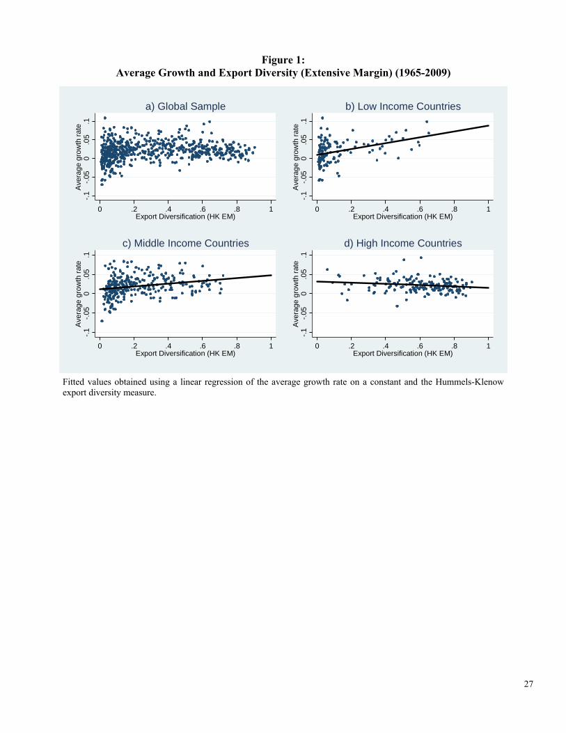
unchanged. The result is not surprising given the partial correlation between growth and export
diversity in the global sample (Figure 1a). On the other hand, we find that the effect of diversity
on growth varies substantially with income (Table 1, Column 3).13 In the presence of the
country-income dummy variables, the main diversity coefficient represents the effect of diversity
on growth for high income countries (the omitted country-income dummy). To obtain the effect
of diversity on growth for the other country-income categories, we construct composite
coefficients that represent the effect of diversity on growth for each remaining income category.
These composite coefficients (“Diversity [LowIncome]”, “Diversity [LowerMedIncome]”,
“Diversity [UpperMedIncome]”) are based on the main effect of “Diversity” and its interaction
with the respective country-income coefficient. The economic effect of diversity, as well as its
statistical significance, decline with development, just as we observe in the partial correlations in
Figures 1b-1d. The economic effect of diversity on low income countries is sizable, implying
that a one standard deviation increase in export diversity raises average annual growth in low
income countries by just about 1 percentage point.14
V.2 2SLS: Controlling for Endogeneity
As outlined in section II, there is ample evidence for feedback effects from growth to trade and
in this section we control for endogeneity by implementing a standard 2SLS approach. Column 4
in Table 1 acknowledges not only the endogeneity of trade, but also the potential endogeneity of
18 other growth determinants whose respective instruments were described in Section II.15 Given
13 The income classifications are coded according to the 1988 World Bank classification (the midpoint of our sample period). Our export diversity results are nearly identical when we use a contemporaneous income classification where countries switch in and out of the income categories. We also estimated a specification in which we fixed countries’ income categories at the time they first entered our panel (1965 or the earliest year thereafter) and we still find evidence for a positive effect of export diversity on economic growth in low income countries (although weaker). Diversity effects by income classification are calculated as the sum of the main export diversity coefficient and the respective country-income interaction with the diversity term. The standard errors of the composite coefficients are calculated using the Delta Method. 14 The coefficient of 0.062 and the 0.16 standard deviation of export diversity for low income countries imply that a one standard deviation increase in diversity will increase growth by 100x0.062x0.16 = 0.992%. 15 Following Durlauf et al. (2008), the endogenous regressors are “InitialGDP”, “Investment”, “PopulationGrowth”, “Education”, “Openness”, “ExecutiveConstraints”, “GovernmentExpenditures”, “Inflation”, “HinduFraction”,
17
the sizable number of endogenous regressors, we report the Angrist-Pischke test statistics that
indicate whether a particular endogenous regressor is identified. The Angrist-Pischke first-stage
chi-squared and F-statistics are tests of underidentification and weak identification, respectively,
which are both rejected at the 5 percent level for all endogenous variables in our specification.
The Sargan-Hansen J-Statistic rejects instrument validity, indicating that more parsimonious
instrumentation specifications may be preferable.16
In terms of significance, the 2SLS results in column 4 mostly overlap with the OLS
results in column 3. Only “Investment”, “ExecutiveConstraints” and “EasternReligionFraction”
lose significance in the 2SLS approach. The loss of significance for “Investment” is worrisome
but not surprising. While “Investment” is seen as a universal growth determinant in theory,
previous panel studies (e.g., Durlauf et al., 2008, and Barro, 2003) also find that its significance
decreases substantially after controlling for endogeneity. Note that “Investment” is insignificant
only when we control for endogeneity, but before we address model uncertainty. Export diversity
remains significant for low (and upper medium) income countries.
V.3 Model Uncertainty, Endogeneity and Export Diversity
The set of candidate regressors in growth regressions is always an amalgam of variables
suggested by a multitude of growth theories. Hence, it is important to control not only for
endogeneity but also for the associated uncertainty whether a regressor suggested by a particular
theory captures the true underlying growth process. Here it is important to note that single
regressions cannot account for the uncertainty surrounding the validity of a particular empirical
model. While an extensive literature on model uncertainty in growth regressions exists, only
Durlauf et al. (2008) account simultaneously for endogeneity and model uncertainty (in the
second stage only). Using IVBMA, we examine whether export diversity exerts an effect on
growth, even after controlling for endogeneity and model uncertainty.17
“EasternReligionFraction”, “OrthodoxFraction”, “MuslimFraction”, “OtherReligionsFraction”, “JewishFraction”, “ProtestantFraction”, “Diversity”, and “Diversity” with three income interactions. Our instruments follow directly from Barro (2003) and Durlauf et al. (2008). 16 A formal Bayesian test for weak instruments does not exist. Lenkoski et al. (2014) suggest a simple and direct approach based on the instruments’ inclusion probabilities. IVBMA addresses the issue of weak instruments by providing negligible inclusion probabilities and low posterior model weights to models with weak instruments. 17 To implement IVBMA, we use Lenkoski’s IVBMA R-package, which relies on a MC3-Within-Gibbs sampler, a uniform model prior and an inverse Wishart prior over the parameter space, see Karl and Lenkoski (2012). The
18
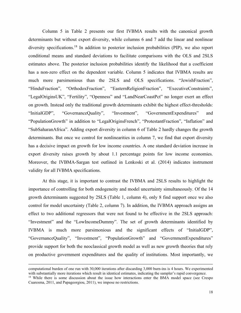
Column 5 in Table 2 presents our first IVBMA results with the canonical growth
determinants but without export diversity, while columns 6 and 7 add the linear and nonlinear
diversity specifications.18 In addition to posterior inclusion probabilities (PIP), we also report
conditional means and standard deviations to facilitate comparisons with the OLS and 2SLS
estimates above. The posterior inclusion probabilities identify the likelihood that a coefficient
has a non-zero effect on the dependent variable. Column 5 indicates that IVBMA results are
much more parsimonious than the 2SLS and OLS specifications. “JewishFraction”,
“HinduFraction”, “OrthodoxFraction”, “EasternReligionFraction”, “ExecutiveConstraints”,
“LegalOriginsUK”, “Fertility”, “Openness” and “LandNearCoastPct” no longer exert an effect
on growth. Instead only the traditional growth determinants exhibit the highest effect-thresholds:
“InitialGDP”, “GovernanceQuality”, “Investment”, “GovernmentExpenditures” and
“PopulationGrowth” in addition to “LegalOriginsFrench”, “ProtestantFraction”, “Inflation” and
“SubSaharanAfrica”. Adding export diversity in column 6 of Table 2 hardly changes the growth
determinants. But once we control for nonlinearities in column 7, we find that export diversity
has a decisive impact on growth for low income countries. A one standard deviation increase in
export diversity raises growth by about 1.1 percentage points for low income economies.
Moreover, the IVBMA-Sargan test outlined in Lenkoski et al. (2014) indicates instrument
validity for all IVBMA specifications.
At this stage, it is important to contrast the IVBMA and 2SLS results to highlight the
importance of controlling for both endogeneity and model uncertainty simultaneously. Of the 14
growth determinants suggested by 2SLS (Table 1, column 4), only 8 find support once we also
control for model uncertainty (Table 2, column 7). In addition, the IVBMA approach assigns an
effect to two additional regressors that were not found to be effective in the 2SLS approach:
“Investment” and the “LowIncomeDummy”. The set of growth determinants identified by
IVBMA is much more parsimonious and the significant effects of “InitialGDP”,
“GovernanceQuality”, “Investment”, “PopulationGrowth” and “GovernmentExpenditures”
provide support for both the neoclassical growth model as well as new growth theories that rely
on productive government expenditures and the quality of institutions. Most importantly, we
computational burden of one run with 30,000 iterations after discarding 3,000 burn-ins is 4 hours. We experimented with substantially more iterations which result in identical estimates, indicating the sampler’s rapid convergence. 18 While there is some discussion about the issue how interactions enter the BMA model space (see Crespo Cuaresma, 2011, and Papageorgiou, 2011), we impose no restrictions.

19
document the crucial effect of trade, through export diversity, that drives growth in low income
countries.
VI. Robustness
In this section, we examine whether our results are sensitive to a) the use of different export
diversity measures, b) the inclusion of additional control variables that might lower the
explanatory power of export diversity, and c) alternative channels through which export diversity
might affect growth. As discussed in section IV, a number of alternative export diversity indices
have been suggested in the literature. Although all measures identify different dimensions of
sectoral export diversity, we show that our IVBMA growth determinants and the effect of export
diversity on growth are remarkably stable across specifications. We also confirm that our results
are robust to the simultaneous inclusion of the extensive and intensive margins of trade, although
we will show that the extensive margin dominates. Then we examine growth determinants that
might negate the explanatory power of export diversity and check if their omission may have
introduced omitted variable bias. Specifically, we investigate whether controlling for the effects
of trade agreements, WTO membership, output volatility, primary exports, the real exchange rate
and a country’s terms-of-trade negates the effect of export diversity on growth. In all cases, our
previous findings are robust. Finally, we examine alternative channels which might amplify the
effect of export diversity on growth (specifically trade openness and primary export shares). We
show that export diversity drives growth in low income economies independent of countries’
trade volumes, while countries relying on primary exports can particularly benefit from
diversification.
VI.1 Alternative Diversity Measures
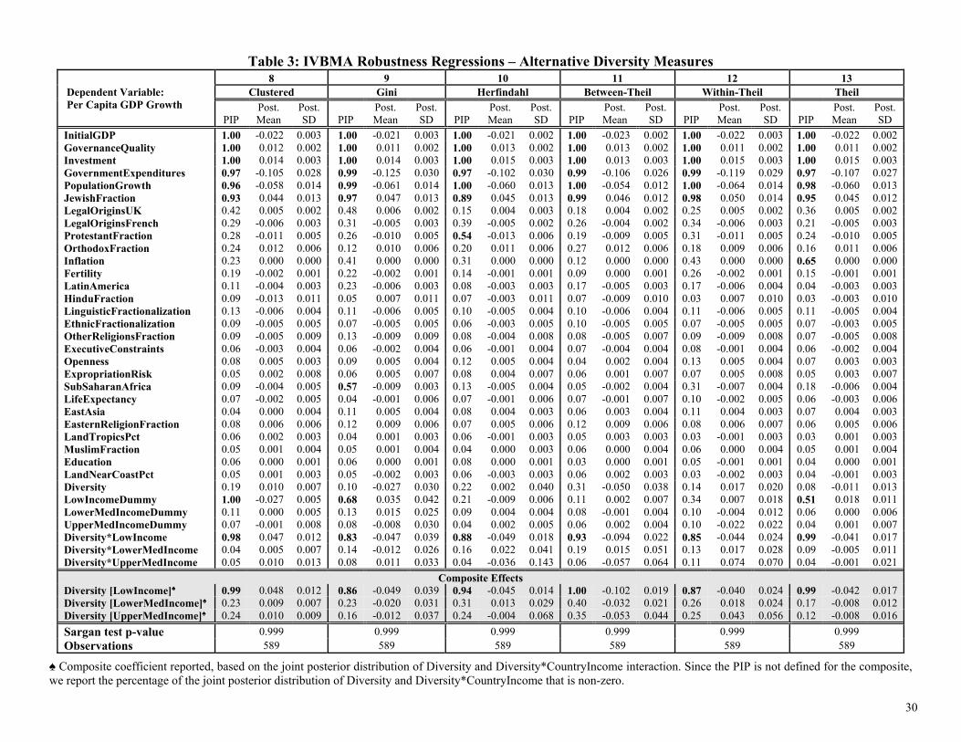
Table 3 presents IVBMA results for six alternative export diversity measures to document the
robustness of our baseline specification. Column 8 reports estimates for the “Clustered” export
diversity measure discussed in section IV, which are just about identical to those produced by
our baseline (Table 2, column 7). This result indicates that the arbitrary nomenclatures of the UN
Comtrade database do not drive our findings. Columns 9-13 present results for the “Herfindahl”,
“Gini” and “Theil” indices, which are very similar to column 8, the only difference being that the
Herfindahl index also attributes a weak effect to a country’s “ProtestantFraction”.
20
VI.2 Intensive versus Extensive Margins
Table 4 presents results that control for the intensive rather than the extensive margin of exports.
Since a number of studies point out that existing export lines are crucial drivers of trade growth
(see Felbermayr and Kohler, 2006, Helpman et al., 2008, and Amiti and Freund, 2010), we also
calculate a measure of export diversity based on the intensive margin
(“IntensiveMarginDiversity”) following Hummels and Klenow (2005, p. 710-711). Again, the
results are very similar to our baseline. Column 14 in Table 4 shows that
“IntensiveMarginDiversity” indeed matters for low income countries, but the effect vanishes
once we include our preferred measure of diversity based on the extensive margin (“Diversity”)
in column 15. Thus, low income countries are pushed up the development ladder by the diversity
of their export sectors, and not by the similarity of their active export sectors' trade volumes.
VI.3 Additional Control Variables
The candidate regressors that are included in our baseline specification were motivated by
traditional growth determinant studies. Table 5 introduces additional control variables that are
specifically linked to export diversity, as discussed in section II. Their omission might lead to
omitted variable bias resulting in an overstatement of the explanatory power of export diversity
on growth. Columns 16-18 in Table 5 add WTO membership (“WTO”), membership in
Preferential Trade Agreements (“PTA”), primary export shares (“PrimaryX”), output volatility
(“GDPVolatility”), the real effective exchange rate (“REER”), real exchange rate volatility
(“FXVolatility”), terms-of-trade (“TOT”) and TOT volatility (“TOTVolatility”). All additional
covariates are treated as exogenous and their inclusion does not change our previous result that
export diversity drives growth in low income countries. Neither of the new variables is identified
as key growth determinant, with the exception of “FXVolatility”, which is shown to exert a
decisive effect on growth. The inclusion of “FXVolatility” does not, however, affect the
diversity-growth relationship. Finally, column 19 introduces “FDIInFlow” and “FDIOutFlow” to
proxy for countries’ global TFP exposure. Only “FDIInFlow” exerts an effect on growth, but the
diversity-growth relationship is again robust.
VI.4 Diversity Catalysts
The effect of diversity might be driven by a third regressor, which would then be the underlying
catalyst of growth. In section II, we motivate how trade openness and primary exports may exert
21
an effect on both diversity and growth. By interacting diversity with “PrimaryX” and
“Openness”, we can examine if the diversity effect is indeed operating through either of these
two potential catalysts. When interacting diversity and openness (Table 6, column 20), we find
no change in our core results, including the estimated coefficient magnitudes. Trade openness
does not drive the export diversity effect on growth in low income countries. Using “PrimaryX”
and “Diversity” interactions, column 21 examines the Prebisch-Singer hypothesis that reliance
on primary exports (implying lower diversity) impacts growth. The positive and significant
effect for the interaction of “PrimaryX” with “Diversity” and the “LowIncomeDummy” provides
evidence that the diversity-growth relationship for low income countries is indeed partly
operating through primary exports. The greater the primary export reliance of a low income
country, the larger is the growth impact of diversification.
VII. Concluding Remarks
We reexamine the effect of trade on growth by conducting a detailed analysis of the impact of
sectoral exports. Since previous empirical studies of growth determinants did not find a robust
trade effect, we introduce disaggregate exports to examine the impact of sectoral export diversity
on growth. Using Hummels and Klenow’s (2005) measure of export diversity, we find decisive
evidence that export diversification is a key determinant of growth in low income countries, an
effect that weakens and eventually vanishes with development. Our findings are robust to the
two major caveats that are generally encountered in growth regressions: endogeneity and model
uncertainty. Our results are also robust to the inclusion of at least five alternative export
diversification measures and a number of variables that have been suggested as potential drivers
of export diversity.
The benefits of export diversity for growth are thus greatest in the early stages of
development. As development progresses, export diversification is shown to be a by-product of
prosperity but not its cause. Export diversity could drive growth in low income countries through
several channels. More diversified economies are, for instance, better insured against
idiosyncratic sectoral shocks, especially at the early stages of development when countries
export only few products. Finally, in the light of our results, it is of interest to note the finding of
Besedes and Prusa (2011) that the extensive margin growth in developing countries is less stable

22
than in developed economies. Since we consider 5-year averages, our findings suggest that short-
run fluctuations in export diversity are less important for low income countries than the steady
diversification of exports over the long run to successfully climb the development ladder.

23
References
Amiti, Mary and Freund, Caroline (2010). “The Anatomy of China's Export Growth.” In: Feenstra, Robert C. and Wei, Shang-Jin (eds), China's Growing Role in World Trade The University of Chicago Press: 35-56.
Baldwin, Richard E. and Robert-Nicoud, Frédéric. (2008). “Trade and Growth With Heterogeneous Firms.” Journal of International Economics, 74(1), 21-34.
Barro, Robert J. (2003). “Determinants of Economic Growth in a Panel of Countries.” Annals of Economics and Finance, 4, 231-274.
Bernhofen, Daniel M. (2011). “The Empirics of General Equilibrium Trade Theory.” In: Bernhofen, Daniel M.; Falvey, Rod; Greenaway, David and Udo Kreickemeier (eds.), Palgrave Handbook of International Trade, Palgrave MacMillan: 88-118.
Besedes, Tibor and Prusa, Thomas J. (2011). “The Role of Extensive and Intensive Margins and Export Growth.” Journal of Development Economics, 96(2), 371-379.
Brasili, Andrea; Epifani, Paolo and Helg, Rodolfo (2000). “On the Dynamics of Trade Patterns.” De Economist, 148(2), 233-257.
Brenton, Paul and Newfarmer, Richard (2007). “Watching More Than the Discovery Channel: Export Cycles and Diversification in Development.” World Bank Policy Research Working Paper 4302.
Brock, William A. and Durlauf, Steven N. (2001). “What Have We Learned From a Decade of Empirical Research on Growth? Growth Empirics and Reality.” World Bank Economic Review, 15(2), 229-272.
Cadot, Olivier; Carrère, Céline and Strauss-Kahn, Vanessa (2011). “Export Diversification: What’s Behind the Hump?” Review of Economics and Statistics, 93(2), 590-605.
Chen, Huigang; Mirestean, Alin and Tsanarides, Charalambos (2009). “Limited Information Bayesian Model Averaging for Dynamic Panels with Short Time Periods.” IMF Working Paper WP/09/74.
Ciccone, Antonio and Jarocinski, Marek (2010). “Determinants of Economic Growth: Will Data Tell?” American Economic Journal: Macroeconomics, 2(4), 222-246.
Cohen-Cole, Ethan; Durlauf, Steven; Fagan, Jeffrey and Nagin, Daniel (2009). “Model Uncertainty and the Deterrent Effect of Capital Punishment.” American Law and Economics Review, 11(2), 335-369.
Crespo Cuaresma, Jesus (2011). “How Different Is Africa? A Comment On Masanjala and Papageorgiou.” Journal of Applied Econometrics, 26(6), 1041-1047.
De Benedictis, Luca; Gallegati, Marco and Tamberi, Massimo (2009). “Overall Trade Specialization and Economic Development: Countries Diversify.” Review of World Economics, 145(1), 37-55.
Dixit, Avinash K. and Norman, Victor D. (1980). Theory of International Trade: A Dual, General Equilibrium Approach. Cambridge, England: Cambridge University Press.
24
Djankov, Simeon; La Porta, Rafael; Lopez-de-Silanes, Florencio and Shleifer, Andrei (2003). “Courts.” Quarterly Journal of Economics, 118(2), 453-517.
Durlauf, Steven N.; Kourtellos, Andros and Tan, Chih Ming (2008). “Are Any Growth Theories Robust?” Economic Journal, 118 (March), 329-346.
Durlauf, Steven N.; Kourtellos, Andros and Tan, Chih Ming (2012). “Is God in the Details? A Reexamination of the Role of Religion in Economic Growth.” Journal of Applied Econometrics, 27(7), 1059-1075.
Edwards, Sebastian (1993). “Openness, Trade Liberalization, and Growth in Developing Countries.” Journal of Economic Literature, 31(3), 1358-1393.
Eicher, Theo S.; Papageorgiou, Chris and Raftery, Adrian E. (2011). “Default Priors and Predictive performance in Bayesian Model Averaging, with Application to growth Determinants.” Journal of Applied Econometrics, 26(1), 30-55.
Eris, Mehmet N. and Ulasan, Bülent (2013). “Trade Openness and Economic Growth: Bayesian Model Averaging Estimate of Cross-country Growth Regressions.” Economic Modelling, 33, 867-883.
Feenstra, Robert C. (1994). “New Product Varieties and the Measurement of International Prices.” American Economic Review, 84(1), 157-177.
Feenstra, Robert C. and Kee, Hiau Looi (2008). “Export Variety and Country Productivity: Estimating the Monopolistic Competition Model with Endogenous Productivity.” Journal of International Economics, 74(2), 500-518.
Feenstra, Robert C.; Lipsey, Robert E., Deng, Haiyan; Ma, Alyson C. and Mo, Hengyong (2005). “World Trade Flows: 1962-2000.” NBER Working Paper 11040.
Felbermayr, Gabriel J., and Kohler, Wilhelm (2006). “Exploring the Intensive and Extensive Margins of World Trade.“ Review of World Economics, 142(4), 642-673.
Fernández, Carmen; Ley, Eduardo and Mark F. J. Steel (2001). “Model Uncertainty in Cross-Country Growth Regressions.” Journal of Applied Econometrics, 16(5), 563-576.
Frankel, Jeffrey A. and Romer, David (1999). “Does Trade Cause Growth?” American Economic Review, 89(3), 379-399.
Funke, Michael and Ruhwedel, Ralf (2001). “Product Variety and Economic Growth: Empirical Evidence for the OECD Countries.” IMF Staff Papers, 48(2), 225-242.
Grossman, Gene M. and Helpman, Elhanan (1991). Innovation and Growth in the Global Economy. Cambridge, MA: MIT Press.
Hausmann, Ricardo and Hidalgo, César A. (2011). “The Network Structure of Economic Output.” Journal of Economic Growth, 16(4), 309-342.
Helpman, Elhanan; Melitz, Marc and Rubinstein, Yona (2008). “Estimating Trade Flows: Trading Partners and Trading Volumes.” Quarterly Journal of Economics, 123(2), 441-487.
Henderson, Daniel J.; Papageorgiou, Chris and Christopher F. Parmeter (2012). “Growth Empirics Without Parameters.” Economic Journal, 122 (March), 125-154.

25
Karl, Anna and Lenkoski, Alex (2012). “Instrumental Variable Bayesian Model Averaging via Conditional Bayes Factors.” Heidelberg University Working Paper.
Kass, Robert E. and Raftery, Adrian E. (1995). “Bayes Factors.” Journal of the American Statistical Association, 90(430), 773-795.
Kass, Robert E. and Wasserman, Larry (1995). “A Reference Bayesian Test for Nested Hypotheses and its Relationship to the Schwarz Criterion.” Journal of the American Statistical Association, 90(431), 928-934.
Kehoe, Timothy J. and Ruhl, Kim J. (2013). “How Important Is the New Goods Margin in International Trade?” Journal of Political Economy, 121(2), 358-392.
Kleibergen, Frank and Zivot, Eric (2003). “Bayesian and Classical Approaches to Instrumental Variable Regression.” Journal of Econometrics, 114(1), 29-72.
Koop, Gary; Leon-Gonzalez, Roberto and Strachan, Rodney (2012). “Bayesian Model Averaging in the Instrumental Variable Regression Model.” Journal of Econometrics, 171(2), 237-250.
Koren, Miklós and Tenreyro, Silvana (2007). “Volatility and Development.” Quarterly Journal of Economics, 122(1), 243-287.
Krugman, Paul (1980). “Scale Economies, Product Differentiation, and the Pattern of Trade.” American Economic Review, 70(5), 950-959.
La Porta, Rafael; Lopez-de-Silanes, Florencio and Shleifer, Andrei (2008). “The Economic Consequences of Legal Origins.” Journal of Economic Literature, 46(2), 285-332.
Leamer, Edward E. (1978). “Specification Searches: Ad Hoc Inference from Non-Experimental Data.” New York, NY: Wiley.
Lenkoski, Alex; Eicher, Theo S. and Raftery, Adrian E. (2014). “Two-Stage Bayesian Model Averaging in Endogenous Variable Models." Econometric Reviews, 33(1-4), 122-151.
Levine, Ross and Renelt, David (1992). “A sensitivity Analysis of Cross-Country Growth Regressions.” American Economic Review, 82(4), 942-963.
Melitz, Marc J (2003). “The Impact of Trade on Intra-Industry Reallocations and Aggregate Industry Productivity.” Econometrica, 71(6), 1695-1725.
Moral-Benito, Enrique (2012). “Determinants of Economic Growth: A Bayesian Panel Data Approach”, Review of Economics and Statistics, 94(2), 566-579.
Moral-Benito, Enrique (2012b). “Growth Empirics in Panel Data under Model Uncertainty and Weak Exogeneity.” Bank of Spain Working Paper 1243.
Parteka, Aleksandra (2010). “Employment and Export Specialisation Along the Development Path: Some Robust Evidence.” Review of World Economics, 145(4), 615-640.
Papageorgiou, Chris (2011). “How To Use Interaction Terms In BMA: Reply To Crespo Cuaresma’s Comment On Masanjala And Papageorgiou (2008).” Journal of Applied Econometrics, 26(6), 1048-1050.
Papageorgiou, Chris and Spatafora, Nikola (2012). “Economic Diversification in LICs: Stylized Facts and Macroeconomic Implications.” IMF Staff Discussion Note SDN/12/13.

26
Prebisch, Raul (1950). The Economic Development of Latin America and its Principal Problems. New York: United Nations.
Proudman, James and Redding, Stephen (2000). “Evolving Patterns of International Trade.” Review of International Economics, 8(3), 373-396.
Raddatz, Claudio (2011). “Over the Hedge: Exchange Rate Volatility, Commodity Price Correlations and the Structure of Trade.” World Bank Policy Research Working Paper 5590.
Raftery, Adrian E. (1995). “Bayesian Model Selection in Social Research.” Sociological Methodology, 25, 111-163.
Raftery, Adrian E. and Zheng, Yingye (2003). “Discussion: Performance of Bayesian Model Averaging.” Journal of the American Statistical Association, 98, 931-938.
Rivera-Batiz, Luis A. and Romer, Paul M. (1991). “Economic Integration and Endogenous Growth.” Quarterly Journal of Economics, 106(2), 531-555.
Rodriguez, Francisco and Rodrik, Dani (2001). “Trade Policy and Economic Growth: A Skeptic’s Guide to the Cross-National Evidence.” In: Bernanke, Ben S. and Rogoff, Kenneth (eds.), NBER Macroeconomics Annual 2000.
Sachs, Jeffrey D. and Warner, Andrew (1995). “Economic Reform and the Process of Global Integration.” Brookings Papers on Economic Activity, Vol. 1, 1-118.
Sala-i-Martin, Xavier X. (1997). “I Just Ran Two Million Regressions.” American Economic Review Papers and Proceedings, 87(2), 178-183.
Sala-i-Martin, Xavier X.; Doppelhofer, Gernot and Miller, Ronald I. (2004). “Determinants of Long-Term Growth: A Bayesian Averaging of Classical Estimates (BACE).” American Economic Review, 94(4), 813-835.
Singer, Hans W. (1950). “The Distribution of Gains between Investing and Borrowing Countries.” American Economic Review Papers and Proceedings, 40(2), 473-485.
Young, Alwyn (1991). “Learning by Doing and the Dynamic Effects of International Trade.” Quarterly Journal of Economics, 106(2), 369-405.
27
Figure 1: Average Growth and Export Diversity (Extensive Margin) (1965-2009)
-.1
-.05
0.0
5.1
Ave
rag
e g
row
th r
ate
0 .2 .4 .6 .8 1Export Diversification (HK EM)
a) Global Sample
-.1
-.05
0.0
5.1
Ave
rag
e g
row
th r
ate
0 .2 .4 .6 .8 1Export Diversification (HK EM)
b) Low Income Countries
-.1
-.05
0.0
5.1
Ave
rag
e g
row
th r
ate
0 .2 .4 .6 .8 1Export Diversification (HK EM)
c) Middle Income Countries
-.1
-.05
0.0
5.1
Ave
rag
e g
row
th r
ate
0 .2 .4 .6 .8 1Export Diversification (HK EM)
d) High Income Countries
Fitted values obtained using a linear regression of the average growth rate on a constant and the Hummels-Klenow export diversity measure.

28
Table 1: OLS and 2SLS Estimates
1 2 3 4 Dependent Variable: Extended DKT Extended DKT Extended DKT Extended DKT Per Capita GDP Growth ols ols ols 2sls (2nd Stage) AP p-values Coeff SE Coeff SE Coeff SE Coeff SE Χ2 F
InitialGDP -0.011*** 0.003 -0.012*** 0.003 -0.015*** 0.004 -0.020*** 0.005 0.000 0.000 GovernanceQuality 0.005*** 0.003 0.006*** 0.003 0.010*** 0.003 0.013*** 0.003 Investment 0.010*** 0.003 0.010*** 0.003 0.011*** 0.003 0.006*** 0.004 0.000 0.000 GovernmentExpenditures -0.107*** 0.026 -0.108*** 0.026 -0.112*** 0.026 -0.133*** 0.039 0.000 0.000 PopulationGrowth -0.042*** 0.012 -0.042*** 0.012 -0.044*** 0.012 -0.058*** 0.023 0.000 0.001 JewishFraction 0.039*** 0.009 0.040*** 0.009 0.035*** 0.009 0.062*** 0.016 0.000 0.000 LegalOriginsUK 0.005*** 0.003 0.004*** 0.003 0.007*** 0.003 0.008*** 0.005 LegalOriginsFrench -0.002*** 0.003 -0.002*** 0.004 -0.002*** 0.004 -0.001*** 0.005 ProtestantFraction -0.007*** 0.004 -0.008*** 0.004 -0.008*** 0.004 -0.010*** 0.006 0.000 0.000 OrthodoxFraction 0.008*** 0.005 0.010*** 0.006 0.006*** 0.006 0.008*** 0.006 0.000 0.000 Inflation -0.000*** 0.000 -0.000*** 0.000 -0.000*** 0.000 -0.000*** 0.000 0.017 0.030 Fertility -0.003*** 0.002 -0.003*** 0.001 -0.002*** 0.002 -0.003*** 0.002 LatinAmerica -0.001*** 0.005 0.001*** 0.005 -0.002*** 0.005 -0.005*** 0.007 HinduFraction -0.001*** 0.012 -0.003*** 0.013 -0.024*** 0.014 -0.028*** 0.017 0.000 0.000 LinguisticFractionalization -0.008*** 0.005 -0.007*** 0.005 -0.002*** 0.006 -0.007*** 0.007 EthnicFractionalization -0.005*** 0.006 -0.006*** 0.006 -0.008*** 0.006 -0.004*** 0.007 OtherReligionsFraction -0.007*** 0.008 -0.007*** 0.008 -0.011*** 0.008 -0.017*** 0.015 0.000 0.000 ExecutiveConstraints -0.006*** 0.004 -0.006*** 0.004 -0.007*** 0.004 -0.003*** 0.005 0.000 0.000 Openness 0.007*** 0.004 0.007*** 0.004 0.003*** 0.004 0.004*** 0.005 0.000 0.000 ExpropriationRisk 0.001*** 0.010 -0.001*** 0.011 -0.007*** 0.011 -0.005*** 0.011 SubSaharanAfrica -0.003*** 0.005 -0.003*** 0.005 -0.000*** 0.006 0.000*** 0.008 LifeExpectancy 0.011*** 0.013 0.012*** 0.013 0.008*** 0.014 0.002*** 0.014 EastAsia 0.005*** 0.004 0.004*** 0.005 -0.006*** 0.005 0.001*** 0.008 EasternReligionFraction 0.005*** 0.006 0.005*** 0.006 0.012*** 0.006 0.001*** 0.009 0.000 0.000 LandTropicsPct 0.003*** 0.004 0.003*** 0.004 0.005*** 0.005 0.003*** 0.005 MuslimFraction 0.000*** 0.004 0.001*** 0.004 -0.002*** 0.005 -0.006*** 0.007 0.000 0.000 Education -0.001*** 0.001 -0.000*** 0.001 -0.001*** 0.001 -0.001*** 0.001 0.000 0.000 LandNearCoastPct -0.007*** 0.004 -0.007*** 0.004 -0.006*** 0.004 -0.009*** 0.004 Diversity 0.007*** 0.008 -0.002*** 0.009 -0.003*** 0.011 0.000 0.000 LowIncomeDummy -0.020*** 0.010 -0.020*** 0.014 LowerMedIncomeDummy -0.005*** 0.009 0.001*** 0.012 UpperMedIncomeDummy -0.011*** 0.010 -0.020*** 0.013 Diversity*LowIncome 0.064*** 0.019 0.065*** 0.030 0.000 0.000 Diversity*LowerMedIncome 0.026*** 0.012 0.007*** 0.018 0.000 0.000 Diversity*UpperMedIncome 0.037*** 0.022 0.059*** 0.029 0.000 0.000
Composite Effects Diversity [LowIncome]♠ 0.062*** 0.019 0.062*** 0.032 Diversity [LowerMedIncome]♠ 0.024*** 0.011 0.004*** 0.017 Diversity [UpperMedIncome]♠ 0.035*** 0.023 0.056*** 0.029
R-squared 0.409 0.410 0.434 0.403 Sargan test p-value 0.000 Observations 589 589 589 589
♠ Composite coefficient comprised of Diversity and Diversity*CountryIncome interaction, standard errors calculated using the Delta Method.

29
Table 2: IVBMA Estimates
5 6 7 Dependent Variable: Extended DKT Extended DKT Extended DKT Per Capita GDP Growth IVBMA IVBMA IVBMA
PIP Post. Mean
Post. SD PIP
Post. Mean
Post. SD PIP
Post. Mean
Post. SD
InitialGDP 1.00 -0.016 0.002 1.00 -0.016 0.002 1.00 -0.022 0.002 GovernanceQuality 1.00 0.010 0.002 1.00 0.011 0.002 1.00 0.011 0.002 Investment 0.99 0.012 0.003 0.99 0.013 0.003 1.00 0.014 0.003 GovernmentExpenditures 0.75 -0.075 0.028 0.85 -0.078 0.032 0.99 -0.112 0.027 PopulationGrowth 0.87 -0.045 0.013 0.84 -0.042 0.014 1.00 -0.062 0.013 JewishFraction 0.23 0.027 0.016 0.27 0.031 0.020 0.98 0.047 0.012 LegalOriginsUK 0.13 0.000 0.004 0.12 0.000 0.005 0.54 0.006 0.002 LegalOriginsFrench 0.65 -0.006 0.002 0.71 -0.006 0.002 0.29 -0.005 0.003 ProtestantFraction 0.92 -0.016 0.005 0.91 -0.016 0.005 0.21 -0.009 0.005 OrthodoxFraction 0.09 0.008 0.006 0.11 0.010 0.006 0.19 0.011 0.006 Inflation 0.59 0.000 0.000 0.33 0.000 0.000 0.19 0.000 0.000 Fertility 0.35 -0.002 0.002 0.34 -0.003 0.001 0.12 -0.001 0.001 LatinAmerica 0.06 -0.002 0.003 0.09 -0.002 0.004 0.13 -0.004 0.003 HinduFraction 0.03 -0.004 0.009 0.06 -0.006 0.009 0.10 -0.016 0.011 LinguisticFractionalization 0.06 -0.004 0.005 0.10 -0.005 0.006 0.10 -0.006 0.004 EthnicFractionalization 0.07 -0.004 0.006 0.07 -0.003 0.005 0.10 -0.004 0.005 OtherReligionsFraction 0.15 0.010 0.012 0.15 0.012 0.011 0.07 -0.005 0.007 ExecutiveConstraints 0.04 0.000 0.004 0.05 0.000 0.005 0.08 -0.003 0.004 Openness 0.04 0.002 0.004 0.08 0.005 0.004 0.10 0.004 0.003 ExpropriationRisk 0.06 -0.001 0.008 0.07 0.000 0.009 0.05 0.002 0.007 SubSaharanAfrica 0.91 -0.011 0.004 0.92 -0.011 0.004 0.06 -0.002 0.004 LifeExpectancy 0.11 -0.003 0.008 0.11 -0.003 0.007 0.03 0.000 0.005 EastAsia 0.12 0.004 0.004 0.07 0.004 0.003 0.05 0.001 0.004 EasternReligionFraction 0.07 0.007 0.007 0.05 0.005 0.007 0.05 0.005 0.006 LandTropicsPct 0.07 0.001 0.003 0.05 0.001 0.003 0.04 0.002 0.003 MuslimFraction 0.06 0.003 0.004 0.06 0.003 0.004 0.04 0.002 0.003 Education 0.06 0.000 0.001 0.04 0.000 0.001 0.04 0.000 0.001 LandNearCoastPct 0.06 -0.002 0.003 0.03 -0.001 0.003 0.04 0.000 0.003 Diversity 0.12 0.008 0.007 0.09 0.006 0.007 LowIncomeDummy 1.00 -0.026 0.005 LowerMedIncomeDummy 0.07 -0.001 0.005 UpperMedIncomeDummy 0.06 -0.003 0.007 Diversity*LowIncome 1.00 0.069 0.016 Diversity*LowerMedIncome 0.05 0.003 0.009 Diversity*UpperMedIncome 0.08 0.012 0.016
Composite Effects Diversity [LowIncome]♠ 1.00 0.070 0.016 Diversity [LowerMedIncome]♠ 0.14 0.005 0.008 Diversity [UpperMedIncome]♠ 0.16 0.010 0.013
Sargan test p-value 0.999 0.999 0.999 Observations 589 589 589
♠ Composite coefficient reported, based on the joint posterior distribution of Diversity and Diversity*CountryIncome interaction. Since the PIP is not defined for the composite, we report the percentage of the joint posterior distribution of Diversity and Diversity*CountryIncome that is non-zero.
30
Table 3: IVBMA Robustness Regressions – Alternative Diversity Measures
8 9 10 11 12 13 Dependent Variable: Per Capita GDP Growth
Clustered Gini Herfindahl Between-Theil Within-Theil Theil
PIP Post. Mean
Post. SD PIP
Post. Mean
Post. SD PIP
Post. Mean
Post. SD PIP
Post. Mean
Post. SD PIP
Post. Mean
Post. SD PIP
Post. Mean
Post. SD
InitialGDP 1.00 -0.022 0.003 1.00 -0.021 0.003 1.00 -0.021 0.002 1.00 -0.023 0.002 1.00 -0.022 0.003 1.00 -0.022 0.002 GovernanceQuality 1.00 0.012 0.002 1.00 0.011 0.002 1.00 0.013 0.002 1.00 0.013 0.002 1.00 0.011 0.002 1.00 0.011 0.002 Investment 1.00 0.014 0.003 1.00 0.014 0.003 1.00 0.015 0.003 1.00 0.013 0.003 1.00 0.015 0.003 1.00 0.015 0.003 GovernmentExpenditures 0.97 -0.105 0.028 0.99 -0.125 0.030 0.97 -0.102 0.030 0.99 -0.106 0.026 0.99 -0.119 0.029 0.97 -0.107 0.027 PopulationGrowth 0.96 -0.058 0.014 0.99 -0.061 0.014 1.00 -0.060 0.013 1.00 -0.054 0.012 1.00 -0.064 0.014 0.98 -0.060 0.013 JewishFraction 0.93 0.044 0.013 0.97 0.047 0.013 0.89 0.045 0.013 0.99 0.046 0.012 0.98 0.050 0.014 0.95 0.045 0.012 LegalOriginsUK 0.42 0.005 0.002 0.48 0.006 0.002 0.15 0.004 0.003 0.18 0.004 0.002 0.25 0.005 0.002 0.36 0.005 0.002 LegalOriginsFrench 0.29 -0.006 0.003 0.31 -0.005 0.003 0.39 -0.005 0.002 0.26 -0.004 0.002 0.34 -0.006 0.003 0.21 -0.005 0.003 ProtestantFraction 0.28 -0.011 0.005 0.26 -0.010 0.005 0.54 -0.013 0.006 0.19 -0.009 0.005 0.31 -0.011 0.005 0.24 -0.010 0.005 OrthodoxFraction 0.24 0.012 0.006 0.12 0.010 0.006 0.20 0.011 0.006 0.27 0.012 0.006 0.18 0.009 0.006 0.16 0.011 0.006 Inflation 0.23 0.000 0.000 0.41 0.000 0.000 0.31 0.000 0.000 0.12 0.000 0.000 0.43 0.000 0.000 0.65 0.000 0.000 Fertility 0.19 -0.002 0.001 0.22 -0.002 0.001 0.14 -0.001 0.001 0.09 0.000 0.001 0.26 -0.002 0.001 0.15 -0.001 0.001 LatinAmerica 0.11 -0.004 0.003 0.23 -0.006 0.003 0.08 -0.003 0.003 0.17 -0.005 0.003 0.17 -0.006 0.004 0.04 -0.003 0.003 HinduFraction 0.09 -0.013 0.011 0.05 0.007 0.011 0.07 -0.003 0.011 0.07 -0.009 0.010 0.03 0.007 0.010 0.03 -0.003 0.010 LinguisticFractionalization 0.13 -0.006 0.004 0.11 -0.006 0.005 0.10 -0.005 0.004 0.10 -0.006 0.004 0.11 -0.006 0.005 0.11 -0.005 0.004 EthnicFractionalization 0.09 -0.005 0.005 0.07 -0.005 0.005 0.06 -0.003 0.005 0.10 -0.005 0.005 0.07 -0.005 0.005 0.07 -0.003 0.005 OtherReligionsFraction 0.09 -0.005 0.009 0.13 -0.009 0.009 0.08 -0.004 0.008 0.08 -0.005 0.007 0.09 -0.009 0.008 0.07 -0.005 0.008 ExecutiveConstraints 0.06 -0.003 0.004 0.06 -0.002 0.004 0.06 -0.001 0.004 0.07 -0.004 0.004 0.08 -0.001 0.004 0.06 -0.002 0.004 Openness 0.08 0.005 0.003 0.09 0.005 0.004 0.12 0.005 0.004 0.04 0.002 0.004 0.13 0.005 0.004 0.07 0.003 0.003 ExpropriationRisk 0.05 0.002 0.008 0.06 0.005 0.007 0.08 0.004 0.007 0.06 0.001 0.007 0.07 0.005 0.008 0.05 0.003 0.007 SubSaharanAfrica 0.09 -0.004 0.005 0.57 -0.009 0.003 0.13 -0.005 0.004 0.05 -0.002 0.004 0.31 -0.007 0.004 0.18 -0.006 0.004 LifeExpectancy 0.07 -0.002 0.005 0.04 -0.001 0.006 0.07 -0.001 0.006 0.07 -0.001 0.007 0.10 -0.002 0.005 0.06 -0.003 0.006 EastAsia 0.04 0.000 0.004 0.11 0.005 0.004 0.08 0.004 0.003 0.06 0.003 0.004 0.11 0.004 0.003 0.07 0.004 0.003 EasternReligionFraction 0.08 0.006 0.006 0.12 0.009 0.006 0.07 0.005 0.006 0.12 0.009 0.006 0.08 0.006 0.007 0.06 0.005 0.006 LandTropicsPct 0.06 0.002 0.003 0.04 0.001 0.003 0.06 -0.001 0.003 0.05 0.003 0.003 0.03 -0.001 0.003 0.03 0.001 0.003 MuslimFraction 0.05 0.001 0.004 0.05 0.001 0.004 0.04 0.000 0.003 0.06 0.000 0.004 0.06 0.000 0.004 0.05 0.001 0.004 Education 0.06 0.000 0.001 0.06 0.000 0.001 0.08 0.000 0.001 0.03 0.000 0.001 0.05 -0.001 0.001 0.04 0.000 0.001 LandNearCoastPct 0.05 0.001 0.003 0.05 -0.002 0.003 0.06 -0.003 0.003 0.06 0.002 0.003 0.03 -0.002 0.003 0.04 -0.001 0.003 Diversity 0.19 0.010 0.007 0.10 -0.027 0.030 0.22 0.002 0.040 0.31 -0.050 0.038 0.14 0.017 0.020 0.08 -0.011 0.013 LowIncomeDummy 1.00 -0.027 0.005 0.68 0.035 0.042 0.21 -0.009 0.006 0.11 0.002 0.007 0.34 0.007 0.018 0.51 0.018 0.011 LowerMedIncomeDummy 0.11 0.000 0.005 0.13 0.015 0.025 0.09 0.004 0.004 0.08 -0.001 0.004 0.10 -0.004 0.012 0.06 0.000 0.006 UpperMedIncomeDummy 0.07 -0.001 0.008 0.08 -0.008 0.030 0.04 0.002 0.005 0.06 0.002 0.004 0.10 -0.022 0.022 0.04 0.001 0.007 Diversity*LowIncome 0.98 0.047 0.012 0.83 -0.047 0.039 0.88 -0.049 0.018 0.93 -0.094 0.022 0.85 -0.044 0.024 0.99 -0.041 0.017 Diversity*LowerMedIncome 0.04 0.005 0.007 0.14 -0.012 0.026 0.16 0.022 0.041 0.19 0.015 0.051 0.13 0.017 0.028 0.09 -0.005 0.011 Diversity*UpperMedIncome 0.05 0.010 0.013 0.08 0.011 0.033 0.04 -0.036 0.143 0.06 -0.057 0.064 0.11 0.074 0.070 0.04 -0.001 0.021
Composite EffectsDiversity [LowIncome]♠ 0.99 0.048 0.012 0.86 -0.049 0.039 0.94 -0.045 0.014 1.00 -0.102 0.019 0.87 -0.040 0.024 0.99 -0.042 0.017 Diversity [LowerMedIncome]♠ 0.23 0.009 0.007 0.23 -0.020 0.031 0.31 0.013 0.029 0.40 -0.032 0.021 0.26 0.018 0.024 0.17 -0.008 0.012 Diversity [UpperMedIncome]♠ 0.24 0.010 0.009 0.16 -0.012 0.037 0.24 -0.004 0.068 0.35 -0.053 0.044 0.25 0.043 0.056 0.12 -0.008 0.016
Sargan test p-value 0.999 0.999 0.999 0.999 0.999 0.999 Observations 589 589 589 589 589 589
♠ Composite coefficient reported, based on the joint posterior distribution of Diversity and Diversity*CountryIncome interaction. Since the PIP is not defined for the composite, we report the percentage of the joint posterior distribution of Diversity and Diversity*CountryIncome that is non-zero.

31
Table 4: IVBMA Robustness Regressions – Extensive versus Intensive Diversity Margins
Dependent Variable: Per Capita GDP Growth
14 15
PIP Post. Mean
Post. SD PIP
Post. Mean
Post. SD
InitialGDP 1.00 -0.022 0.003 1.00 -0.022 0.003 GovernanceQuality 1.00 0.012 0.002 1.00 0.012 0.002 Investment 0.65 0.010 0.004 0.97 0.013 0.003 GovernmentExpenditures 0.98 -0.113 0.030 0.99 -0.107 0.027 PopulationGrowth 0.91 -0.052 0.019 0.98 -0.059 0.015 JewishFraction 0.93 0.046 0.013 0.98 0.045 0.012 LegalOriginsUK 0.43 0.006 0.003 0.52 0.006 0.002 LegalOriginsFrench 0.38 -0.006 0.003 0.23 -0.005 0.003 ProtestantFraction 0.31 -0.012 0.005 0.18 -0.009 0.005 OrthodoxFraction 0.13 0.010 0.006 0.30 0.013 0.006 Inflation 0.66 0.000 0.000 0.31 0.000 0.000 Fertility 0.77 -0.004 0.001 0.25 -0.002 0.001 LatinAmerica 0.15 -0.004 0.004 0.12 -0.005 0.003 HinduFraction 0.06 -0.006 0.012 0.11 -0.016 0.011 LinguisticFractionalization 0.13 -0.006 0.005 0.17 -0.006 0.004 EthnicFractionalization 0.05 -0.004 0.005 0.09 -0.005 0.005 OtherReligionsFraction 0.22 -0.014 0.008 0.07 -0.007 0.008 ExecutiveConstraints 0.07 -0.002 0.005 0.09 -0.003 0.004 Openness 0.07 0.003 0.004 0.08 0.004 0.003 ExpropriationRisk 0.04 0.001 0.008 0.05 0.001 0.008 SubSaharanAfrica 0.11 -0.005 0.004 0.07 -0.002 0.004 LifeExpectancy 0.08 0.000 0.006 0.06 0.000 0.004 EastAsia 0.04 0.001 0.004 0.04 0.001 0.004 EasternReligionFraction 0.07 0.004 0.007 0.07 0.006 0.007 LandTropicsPct 0.03 0.001 0.004 0.06 0.000 0.003 MuslimFraction 0.05 0.000 0.004 0.03 0.002 0.003 Education 0.06 0.000 0.001 0.04 0.000 0.001 LandNearCoastPct 0.07 0.003 0.003 0.07 0.002 0.003 Diversity 0.14 0.006 0.008 IntensiveMarginDiversity 0.05 0.018 0.039 0.06 0.028 0.042 LowIncomeDummy 0.99 -0.034 0.007 1.00 -0.026 0.006 LowerMedIncomeDummy 0.10 0.000 0.007 0.07 0.001 0.005 UpperMedIncomeDummy 0.10 -0.006 0.010 0.16 -0.009 0.009 Diversity*LowIncome 0.92 0.072 0.018 Diversity*LowerMedIncome 0.07 0.006 0.010 Diversity*UpperMedIncome 0.08 0.005 0.025 Int.Marg.Diversity*LowIncome 0.98 1.355 0.403 0.17 0.584 0.848 Int.Marg.Diversity*LowerMedIncome 0.12 0.266 0.220 0.07 0.098 0.220 Int.Marg.Diversity*UpperMedIncome 0.14 0.605 0.499 0.16 0.699 0.506
Composite EffectDiversity [LowIncome]♠ 0.94 0.071 0.020 Diversity [LowerMedIncome]♠ 0.20 0.007 0.009 Diversity [UpperMedIncome]♠ 0.20 0.006 0.017 Int.Marg.Diversity [LowIncome]♠ 0.98 1.354 0.406 0.21 0.470 0.787 Int.Marg.Diversity [LowerMedIncome]♠ 0.16 0.199 0.219 0.13 0.066 0.166 Int.Marg.Diversity [UpperMedIncome]♠ 0.18 0.472 0.504 0.21 0.522 0.525
Sargan test p-value 0.999 0.999 Observations 589 589
♠ Composite coefficient reported, based on the joint posterior distribution of Diversity (IntensiveMarginDiversity) and Diversity*CountryIncome (IntensiveMarginDiversity*CountryIncome) interaction. Since the PIP is not defined for the composite, we report the percentage of the joint posterior distribution of Diversity and Diversity*CountryIncome (IntensiveMarginDiversity and IntensiveMarginDiversity*CountryIncome) that is non-zero.

32
Table 5: IVBMA Robustness Regressions – Additional Control Variables
Dependent Variable: Per Capita GDP Growth
16 17 18 19
PIP Post. Mean
Post. SD PIP
Post. Mean
Post. SD PIP
Post. Mean
Post. SD PIP
Post. Mean
Post. SD
InitialGDP 1.00 -0.021 0.003 1.00 -0.020 0.003 1.00 -0.020 0.003 1.00 -0.022 0.003 GovernanceQuality 1.00 0.012 0.002 1.00 0.010 0.002 0.76 0.008 0.003 1.00 0.013 0.003 Investment 0.99 0.013 0.003 0.99 0.012 0.003 0.95 0.013 0.004 1.00 0.015 0.003 GovernmentExpenditures 0.89 -0.109 0.028 0.89 -0.093 0.028 0.86 -0.103 0.033 1.00 -0.132 0.029 PopulationGrowth 0.95 -0.056 0.014 0.96 -0.054 0.015 0.97 -0.072 0.019 1.00 -0.053 0.014 JewishFraction 0.86 0.046 0.012 0.86 0.043 0.012 0.66 0.047 0.016 0.98 0.051 0.013 LegalOriginsUK 0.34 0.005 0.002 0.42 0.005 0.003 0.34 0.009 0.004 0.43 0.006 0.002 LegalOriginsFrench 0.40 -0.005 0.002 0.47 -0.006 0.003 0.75 -0.010 0.004 0.36 -0.005 0.002 ProtestantFraction 0.35 -0.010 0.005 0.37 -0.011 0.005 0.44 -0.017 0.008 0.11 -0.008 0.006 OrthodoxFraction 0.19 0.012 0.006 0.15 0.010 0.006 0.20 0.015 0.009 0.13 0.011 0.006 Inflation 0.33 0.000 0.000 0.13 0.000 0.000 0.09 0.000 0.000 0.15 0.000 0.000 Fertility 0.25 -0.002 0.001 0.29 -0.002 0.002 0.20 -0.003 0.002 0.07 0.000 0.001 LatinAmerica 0.13 -0.005 0.003 0.06 -0.001 0.004 0.09 -0.004 0.005 0.22 -0.006 0.003 HinduFraction 0.11 -0.014 0.011 0.15 -0.019 0.011 0.35 -0.027 0.012 0.12 -0.010 0.012 LinguisticFractionalization 0.13 -0.007 0.004 0.19 -0.007 0.004 0.16 -0.009 0.005 0.18 -0.008 0.004 EthnicFractionalization 0.08 -0.005 0.005 0.11 -0.006 0.005 0.11 -0.006 0.006 0.08 -0.007 0.005 OtherReligionsFraction 0.09 -0.004 0.007 0.08 -0.001 0.008 0.07 0.004 0.011 0.06 -0.006 0.008 ExecutiveConstraints 0.08 -0.003 0.004 0.12 -0.005 0.004 0.09 -0.005 0.006 0.08 -0.003 0.005 Openness 0.07 0.004 0.004 0.07 0.003 0.004 0.07 -0.001 0.004 0.04 -0.001 0.004 ExpropriationRisk 0.05 0.001 0.008 0.09 -0.002 0.008 0.07 0.000 0.009 0.06 0.001 0.007 SubSaharanAfrica 0.07 -0.003 0.004 0.09 -0.004 0.004 0.13 -0.004 0.006 0.10 -0.005 0.004 LifeExpectancy 0.06 0.001 0.007 0.09 -0.003 0.006 0.13 -0.003 0.006 0.08 -0.002 0.003 EastAsia 0.07 0.000 0.004 0.06 0.004 0.004 0.07 0.000 0.007 0.03 -0.003 0.005 EasternReligionFraction 0.09 0.005 0.007 0.16 0.011 0.006 0.23 0.014 0.009 0.08 0.004 0.007 LandTropicsPct 0.04 0.002 0.003 0.10 0.003 0.003 0.13 0.005 0.004 0.05 0.001 0.004 MuslimFraction 0.06 0.000 0.004 0.02 0.000 0.004 0.07 0.004 0.004 0.06 0.003 0.004 Education 0.05 0.000 0.001 0.06 0.000 0.001 0.08 -0.001 0.001 0.09 -0.001 0.001 LandNearCoastPct 0.03 0.001 0.003 0.06 0.002 0.003 0.04 0.003 0.004 0.08 0.002 0.003 Diversity 0.08 0.007 0.007 0.10 0.005 0.007 0.15 0.012 0.010 0.11 0.007 0.008 LowIncomeDummy 1.00 -0.025 0.005 1.00 -0.023 0.005 0.99 -0.025 0.006 1.00 -0.025 0.005 LowerMedIncomeDummy 0.08 0.000 0.005 0.08 0.001 0.004 0.15 -0.005 0.006 0.09 -0.003 0.004 UpperMedIncomeDummy 0.05 -0.001 0.007 0.02 -0.001 0.007 0.07 0.004 0.006 0.04 -0.002 0.007 Diversity*LowIncome 1.00 0.067 0.016 1.00 0.073 0.017 0.97 0.067 0.022 0.99 0.065 0.016 Diversity*LowerMedIncome 0.03 0.005 0.009 0.03 0.003 0.008 0.08 -0.003 0.013 0.06 -0.001 0.009 Diversity*UpperMedIncome 0.10 0.015 0.018 0.06 0.009 0.013 0.10 0.015 0.012 0.05 0.012 0.016 WTO 0.04 0.002 0.003 0.04 0.002 0.003 0.05 -0.001 0.003 PTA 0.05 0.000 0.000 0.04 0.000 0.000 0.11 0.000 0.000 PrimaryX 0.07 0.002 0.004 0.08 0.006 0.004 0.08 0.005 0.006 GDPVolatility 0.06 -0.031 0.034 0.04 0.002 0.037 0.06 0.010 0.045 REER 0.07 0.002 0.002 0.05 0.002 0.004 FXVolatility 0.99 -0.004 0.001 0.76 -0.003 0.001 TOT 0.05 0.002 0.003 TOTVolatility 0.07 -0.001 0.001 FDIOutFlow 0.08 -0.001 0.001 FDIInFlow 0.95 0.001 0.000
Composite Effects Diversity [LowIncome]♠ 1.00 0.069 0.017 1.00 0.073 0.017 0.99 0.068 0.023 0.99 0.066 0.016 Diversity [LowerMedIncome]♠ 0.11 0.005 0.008 0.13 0.004 0.008 0.22 0.007 0.013 0.15 0.005 0.009 Diversity [UpperMedIncome]♠ 0.17 0.009 0.012 0.16 0.006 0.010 0.24 0.014 0.011 0.15 0.009 0.012
Sargan test p-value 0.999 0.999 0.999 0.999 Observations 589 584 407 541
♠ Composite coefficient reported, based on the joint posterior distribution of Diversity and Diversity*CountryIncome interaction. Since the PIP is not defined for the composite, we report the percentage of the joint posterior distribution of Diversity and Diversity*CountryIncome that is non-zero.

33
Table 6: IVBMA Robustness Regressions – Diversity Catalysts
20 21 Dependent Variable: Diversity via Trade
Openness? Diversity via Primary
Exports? Per Capita GDP Growth
PIP Post. Mean
Post. SD
PIP Post. Mean
Post. SD
Initial GDP 1.00 -0.020 0.002 1.00 -0.021 0.003 GovernanceQuality 1.00 0.012 0.002 1.00 0.012 0.002 Investment 0.98 0.012 0.003 0.97 0.012 0.003 GovernmentExpenditures 0.95 -0.105 0.028 1.00 -0.121 0.028 PopulationGrowth 0.88 -0.048 0.015 0.94 -0.055 0.016 JewishFraction 0.90 0.044 0.013 0.99 0.050 0.012 LegalOriginsUK 0.28 0.005 0.003 0.46 0.006 0.002 LegalOriginsFrench 0.46 -0.006 0.002 0.24 -0.005 0.003 ProtestantFraction 0.28 -0.010 0.005 0.13 -0.008 0.005 OrthodoxFraction 0.40 0.013 0.006 0.17 0.011 0.006 Inflation 0.31 0.000 0.000 0.35 0.000 0.000 Fertility 0.32 -0.002 0.001 0.28 -0.002 0.001 LatinAmerica 0.08 -0.003 0.003 0.30 -0.007 0.004 HinduFraction 0.12 -0.016 0.011 0.06 -0.014 0.011 LinguisticFractionalization 0.11 -0.006 0.004 0.39 -0.011 0.005 EthnicFractionalization 0.14 -0.007 0.005 0.16 -0.007 0.006 OtherReligionsFraction 0.04 -0.004 0.007 0.13 -0.010 0.008 ExecutiveConstraints 0.09 -0.004 0.004 0.06 -0.001 0.004 ExpropriationRisk 0.06 0.004 0.007 0.04 0.001 0.008 SubSaharanAfrica 0.09 -0.003 0.004 0.04 -0.002 0.004 LifeExpectancy 0.07 -0.005 0.009 0.06 -0.003 0.007 EastAsia 0.03 0.000 0.004 0.07 -0.004 0.005 EasternReligionFraction 0.07 0.007 0.007 0.10 0.009 0.008 LandTropicsPct 0.07 0.002 0.003 0.07 -0.001 0.003 MuslimFraction 0.03 0.000 0.003 0.08 0.002 0.005 Education 0.05 0.000 0.001 0.08 0.000 0.001 LandNearCoastPct 0.03 0.001 0.003 0.06 -0.002 0.003 Diversity 0.10 0.005 0.007 0.14 0.006 0.008 LowIncomeDummy 1.00 -0.025 0.005 1.00 -0.028 0.007 LowerMedIncomeDummy 0.10 -0.003 0.005 0.09 -0.001 0.005 UpperMedIncomeDummy 0.06 0.000 0.005 0.09 -0.007 0.011 Diversity*LowIncome 1.00 0.074 0.015 0.40 0.068 0.038 Diversity*LowerMedIncome 0.04 -0.001 0.010 0.06 0.002 0.012 Diversity*UpperMedIncome 0.05 0.010 0.013 0.08 0.013 0.022 Openness 0.07 0.005 0.005 0.09 0.005 0.003 Openness*Diversity 0.07 -0.002 0.012 Openness*LowIncome 0.08 0.010 0.013 Openness*LowerMedIncome 0.04 -0.002 0.006 Openness*UpperMedIncome 0.05 0.015 0.021 Openness*Low*Diversity 0.08 0.060 0.058 Openness*LowerMed*Diversity 0.05 -0.011 0.014 Openness*UpperMed*Diversity 0.07 -0.023 0.051 PrimaryX 0.05 0.000 0.005 PrimaryX*Diversity 0.08 0.015 0.016 PrimaryX*LowIncome 0.19 0.010 0.013 PrimaryX*LowerMedIncome 0.06 -0.004 0.006 PrimaryX*UpperMedIncome 0.07 -0.006 0.019 PrimaryX*Low*Diversity 0.74 0.154 0.071 PrimaryX*LowerMed*Diversity 0.09 0.022 0.032 PrimaryX*UpperMed*Diversity 0.10 0.062 0.061
Composite Effects Diversity [LowIncome, Openness]♠ 1.00 0.075 0.015 Diversity [LowerMedIncome, Openness]♠ 0.24 0.002 0.008 Diversity [UpperMedIncome, Openness]♠ 0.26 0.005 0.009 Diversity [LowIncome, PrimaryX]♠ 1.00 0.054 0.043 Diversity [LowerMedIncome, PrimaryX,♠ 0.32 0.005 0.009 Diversity [UpperMedIncome, PrimaryX]♠ 0.35 0.007 0.013
Sargan test p-value 0.999 0.999 Observations 589 589
♠ Composite coefficient reported, based on the joint posterior distribution of Diversity, Diversity*Catalyst, Diversity*CountryIncome and Diversity*CountryIncome*Catalyst interactions. Since the PIP is not defined for the composite, we report the percentage of the joint posterior distribution of Diversity, Diversity*Catalyst, Diversity*CountryIncome and Diversity*CountryIncome*Catalyst that is non-zero.

34
Data Appendix
Variable Name Mean StDev Min Max Definition Source
Between Theil 0.103 0.100 0.000 0.550
Average Between Theil measure of export diversifications, calculated using 4-digit SITC data (for 1960-1989) and 6-digit HS data (1990-2009).
Authors' own calculations, trade data: Feenstra et al. (2005), Comtrade
EastAsia 0.105 0.307 0.000 1.000 Dummy variable for East Asia. World Bank
EasternReligionFraction 0.055 0.187 0.000 0.967
Eastern Religion share in 1970, 1980, 1990, 2000 as fraction of the population who expressed adherence to some religion and corresponding share in 1900.
Durlauf, Kourtellos, Tan (EJ 2008) for 1900, 1970, 1980, 1990 and McCleary for 2000
Education -3.769 1.864 -11.555 -0.488
Logarithm of the average percentage of a country’s working age population that attended secondary school times the completion rate of secondary school for all periods.
Barro and Lee dataset
Diversity 0.305 0.258 0.008 0.904
Average Hummels-Klenow extensive margin measure of a country's exports, calculated using 4-digit SITC data (for 1960-1989) and 6-digit HS data (1990-2009).
Authors' own calculations, trade data: Feenstra et al. (2005), Comtrade
EthnicFractionalization 0.400 0.261 0.002 0.930 Measures the degree of tension within a country attributable to racial, nationality, or language divisions.
Alesina (2003)
ExecutiveConstraints 0.633 0.352 0.000 1.000
A measure of the extent of institutionalized constraints on the decision making powers of chief executives. This variable ranges from one to seven where higher values equal a greater extent of institutionalized constraints on the power of chief executives. This variable is calculated as per period average. The variable was transformed first using (x-1)/6.
Henderson, Papageorgiou, Parmeter (EJ 2012) and Polity IV Project
ExpropriationRisk 0.718 0.206 0.160 1.000
Risk of “outright confiscation and forced nationalization" of property. Rescaled, from 0 to 1, with a higher score indicating less risk of expropriation.
Henderson, Papageorgiou, Parmeter (EJ 2012) and Durlauf, Kourtellos, Tan (EJ 2008).
Fertility 3.575 2.104 0.073 8.072 Logarithm of the total fertility rate in initial years of 5-year periods.
Henderson, Papageorgiou, Parmeter (EJ 2012) and World Bank.
FDIInFlow 1.922 2.369 -3.433 19.053 Inward FDI flows as percent of GDP UNCTAD FDIOutFlow 0.748 1.729 -0.377 16.782 Outward FDI flows as percent of GDP UNCTAD
g 0.020 0.025 -0.070 0.109 Average per capita GDP growth rate. Henderson, Papageorgiou, Parmeter (EJ 2011 - PWT 6.2), PWT 7.1.
Gini 0.942 0.058 0.699 0.999
Average Gini measure of export diversification, calculated using 4-digit SITC data (for 1960-1989) and 6-digit HS data (1990-2009).
Authors' own calculations, trade data: Feenstra et al. (2005), Comtrade
GovernanceQuality 0.338 0.912 -1.870 1.930
Average Composite Governance index. It is calculated as the average of six variables: voice and accountability, political stability and absence of violence, government effectiveness, regulatory quality, rule of law, and control of corruption.
World Bank
GovernmentExpenditures 0.149 0.054 0.041 0.387 Average ratio of government consumption to GDP.
World Bank.
Herfindahl 0.125 0.154 0.002 0.859
Average Herfindahl measure of export diversification, calculated using 4-digit SITC data (for 1960-1989) and 6-digit HS data (1990-2009).
Authors' own calculations, trade data: Feenstra et al. (2005), Comtrade
HinduFraction 0.019 0.100 0.000 0.820 Hindu share in 1970, 1980, 1990 and 2000 as fraction of the population who expressed adherence to some religion.
Durlauf, Kourtellos, Tan (EJ 2008) for 1900, 1970, 1980, 1990 and McCleary for 2000
Inflation 13.067 23.325 -3.079 270.651 The average consumer price inflation rate.
Henderson, Papageorgiou, Parmeter (EJ 2012) and World Bank.

35
Variable Name Mean StDev Min Max Definition Source
InitialGDP 8.539 1.090 6.177 10.806 Logarithm of initial per capita GDP in each period.
Henderson, Papageorgiou, Parmeter (EJ 2011 - PWT 6.2), PWT 7.1.
IntensiveMarginDiversity 0.023 0.033 0.000 0.267
Average Hummels-Klenow intensive margin measure of a country's exports, calculated using 4-digit SITC data (for 1960-1989) and 6-digit HS data (1990-2009).
Authors' own calculations, trade data: Feenstra et al. (2005), Comtrade
Investment 2.746 0.538 1.097 4.515 Average ratio of investment to GDP. Henderson, Papageorgiou, Parmeter (EJ 2011), PWT 7.1.
JewishFraction 0.015 0.103 0.000 0.896 Jewish share in 1970, 1980, 1990 and 2000 as fraction of the population who expressed adherence to some religion.
Durlauf, Kourtellos, Tan (EJ 2008) for 1900, 1970, 1980, 1990 and McCleary for 2000
LandNearCoastPct 0.504 0.347 0.000 1.000 Percentage of a country’s land area within 100km of an ice-free coast.
Henderson, Papageorgiou, Parmeter (EJ 2011).
LandTropicsPct 0.308 0.395 0.000 1.000 Percentage of land area classified as tropical and subtropical via the in Koeppen-Geiger system.
Henderson, Papageorgiou, Parmeter (EJ 2011).
LatinAmerica 0.233 0.423 0.000 1.000 Dummy variable for Latin America and the Caribbean.
World Bank
LegalOriginsFrench 0.472 0.500 0.000 1.000 Dummy variable that takes value 1 if a country legal system is based on French legal code.
Durlauf, Kourtellos, Tan (EJ 2008).
LegalOriginsUK 0.345 0.476 0.000 1.000 Dummy variable that takes value 1 if a country legal system is based on British legal code.
Durlauf, Kourtellos, Tan (EJ 2008).
LifeExpectancy 0.205 0.497 0.012 2.253 Reciprocal of life expectancy at age 1 in initial years of 5-year periods.
Henderson, Papageorgiou, Parmeter (EJ 2012) and World Bank.
LinguisticFractionalization 0.354 0.304 0.000 0.923 Measure of linguistic fractionalization based on data describing shares of languages spoken as “mother tongues”.
Henderson, Papageorgiou, Parmeter (EJ 2012) and Alesina (2003).
LowerMedIncomeDummy 0.399 0.490 0.000 1.000 Dummy variable taking value one for lower medium income dummies using 1988 World Bank definition.
World Bank
LowIncomeDummy 0.219 0.414 0.000 1.000 Dummy variable taking value one for low income dummies using 1988 World Bank definition.
World Bank
MuslimFraction 0.191 0.330 0.000 0.995 Muslim share in 1970, 1980, 1990 and 2000 as fraction of the population who expressed adherence to some religion.
Durlauf, Kourtellos, Tan (EJ 2008) for 1900, 1970, 1980, 1990 and McCleary for 2000
PTA 10.131 10.687 0.000 56.000 Number of economic integration agreements at the beginning of each period.
NSF-Kellogg Institute EIA database.
Openness -0.035 0.303 -0.505 1.497 Average ratio exports plus imports to GDP, filtered for the relation of this ratio to the logs of population and area.
Openness, GDP, population and area data from PWT 7.1 and World Bank.
OrthodoxFraction 0.037 0.157 0.000 0.972 Orthodox share in 1970, 1980, 1990 and 2000 as fraction of the population who expressed adherence to some religion.
Durlauf, Kourtellos, Tan (EJ 2008) for 1900, 1970, 1980, 1990 and McCleary for 2000
OtherReligionsFraction 0.109 0.182 -0.560 0.904
Other Religion share in 1970, 1980, 1990 and 2000 as fraction of the population who expressed adherence to some religion.
Durlauf, Kourtellos, Tan (EJ 2008) for 1900, 1970, 1980, 1990 and McCleary for 2000
GDPVolatility 0.033 0.025 0.003 0.244 Standard deviation of per capita GDP growth rates during each period.
Authors' own calculations, growth rate data: Henderson, Papageorgiou, Parmeter (EJ 2011 - PWT 6.2), PWT 7.1.
PopulationGrowth -2.718 0.164 -3.201 -2.204 Logarithm of average population growth rate plus 0.05.
Henderson, Papageorgiou, Parmeter (EJ 2011), PWT 7.1.
PrimaryX 0.536 0.298 0.023 0.992
Average share of primary exports in total exports. Primary exports are defined as categories 0, 1, 2, 3, 4 and 68 in SITC (Rev.1) classification.
Authors' own calculations, trade data: Comtrade
ProtestantFraction 0.153 0.259 -0.007 1.460 Protestant share in 1970, 1980, 1990 and 2000 as fraction of the population who expressed adherence to some religion.
Durlauf, Kourtellos, Tan (EJ 2008) for 1900, 1970, 1980, 1990 and McCleary for 2000
REER 4.698 0.455 3.306 9.567 Average real effective exchange rate. Bruegel real effective exchange rate database
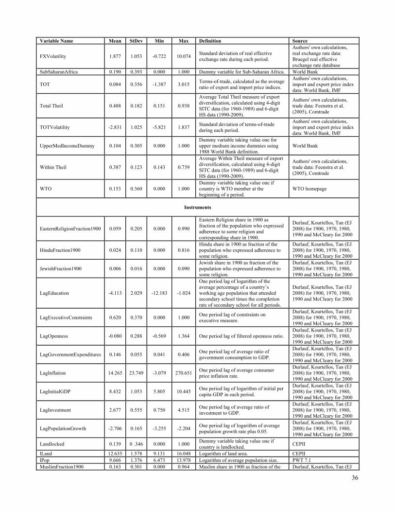
36
Variable Name Mean StDev Min Max Definition Source
FXVolatility 1.877 1.053 -0.722 10.074 Standard deviation of real effective exchange rate during each period.
Authors' own calculations, real exchange rate data: Bruegel real effective exchange rate database
SubSaharanAfrica 0.190 0.393 0.000 1.000 Dummy variable for Sub-Saharan Africa. World Bank
TOT 0.084 0.356 -1.387 3.015 Terms-of-trade, calculated as the average ratio of export and import price indices.
Authors' own calculations, import and export price index data: World Bank, IMF
Total Theil 0.488 0.182 0.151 0.938
Average Total Theil measure of export diversification, calculated using 4-digit SITC data (for 1960-1989) and 6-digit HS data (1990-2009).
Authors' own calculations, trade data: Feenstra et al. (2005), Comtrade
TOTVolatility -2.831 1.025 -5.821 1.837 Standard deviation of terms-of-trade during each period.
Authors' own calculations, import and export price index data: World Bank, IMF
UpperMedIncomeDummy 0.104 0.305 0.000 1.000 Dummy variable taking value one for upper medium income dummies using 1988 World Bank definition.
World Bank
Within Theil 0.387 0.123 0.143 0.739
Average Within Theil measure of export diversification, calculated using 4-digit SITC data (for 1960-1989) and 6-digit HS data (1990-2009).
Authors' own calculations, trade data: Feenstra et al. (2005), Comtrade
WTO 0.153 0.360 0.000 1.000 Dummy variable taking value one if country is WTO member at the beginning of a period.
WTO homepage
Instruments
EasternReligionFraction1900 0.059 0.205 0.000 0.990
Eastern Religion share in 1900 as fraction of the population who expressed adherence to some religion and corresponding share in 1900.
Durlauf, Kourtellos, Tan (EJ 2008) for 1900, 1970, 1980, 1990 and McCleary for 2000
HinduFraction1900 0.024 0.110 0.000 0.816 Hindu share in 1900 as fraction of the population who expressed adherence to some religion.
Durlauf, Kourtellos, Tan (EJ 2008) for 1900, 1970, 1980, 1990 and McCleary for 2000
JewishFraction1900 0.006 0.016 0.000 0.090 Jewish share in 1900 as fraction of the population who expressed adherence to some religion.
Durlauf, Kourtellos, Tan (EJ 2008) for 1900, 1970, 1980, 1990 and McCleary for 2000
LagEducation -4.113 2.029 -12.183 -1.024
One period lag of logarithm of the average percentage of a country’s working age population that attended secondary school times the completion rate of secondary school for all periods.
Durlauf, Kourtellos, Tan (EJ 2008) for 1900, 1970, 1980, 1990 and McCleary for 2000
LagExecutiveConstraints 0.620 0.370 0.000 1.000 One period lag of constraints on executive measure.
Durlauf, Kourtellos, Tan (EJ 2008) for 1900, 1970, 1980, 1990 and McCleary for 2000
LagOpenness -0.080 0.288 -0.569 1.364 One period lag of filtered openness ratio. Durlauf, Kourtellos, Tan (EJ 2008) for 1900, 1970, 1980, 1990 and McCleary for 2000
LagGovernmentExpenditures 0.146 0.055 0.041 0.406 One period lag of average ratio of government consumption to GDP.
Durlauf, Kourtellos, Tan (EJ 2008) for 1900, 1970, 1980, 1990 and McCleary for 2000
LagInflation 14.265 23.749 -3.079 270.651 One period lag of average consumer price inflation rate.
Durlauf, Kourtellos, Tan (EJ 2008) for 1900, 1970, 1980, 1990 and McCleary for 2000
LagInitialGDP 8.432 1.053 5.805 10.445 One period lag of logarithm of initial per capita GDP in each period.
Durlauf, Kourtellos, Tan (EJ 2008) for 1900, 1970, 1980, 1990 and McCleary for 2000
LagInvestment 2.677 0.555 0.750 4.515 One period lag of average ratio of investment to GDP.
Durlauf, Kourtellos, Tan (EJ 2008) for 1900, 1970, 1980, 1990 and McCleary for 2000
LagPopulationGrowth -2.706 0.165 -3.255 -2.204 One period lag of logarithm of average population growth rate plus 0.05.
Durlauf, Kourtellos, Tan (EJ 2008) for 1900, 1970, 1980, 1990 and McCleary for 2000
Landlocked 0.139 0 .346 0.000 1.000 Dummy variable taking value one if country is landlocked.
CEPII
lLand 12.635 1.578 9.131 16.048 Logarithm of land area. CEPII lPop 9.666 1.376 6.473 13.978 Logarithm of average population size. PWT 7.1 MuslimFraction1900 0.163 0.301 0.000 0.964 Muslim share in 1900 as fraction of the Durlauf, Kourtellos, Tan (EJ

37
population who expressed adherence to some religion.
2008) for 1900, 1970, 1980, 1990 and McCleary for 2000
Variable Name Mean StDev Min Max Definition Source
OrthodoxFraction1900 0.041 0.163 0.000 0.982 Orthodox share in 1900 as fraction of the population who expressed adherence to some religion.
Durlauf, Kourtellos, Tan (EJ 2008) for 1900, 1970, 1980, 1990 and McCleary for 2000
OtherReligionsFraction1900 0.206 0.326 0.000 0.997 Other Religion share in 1900 as fraction of the population who expressed adherence to some religion.
Durlauf, Kourtellos, Tan (EJ 2008) for 1900, 1970, 1980, 1990 and McCleary for 2000
ProtestantFraction1900 0.150 0.301 0.000 0.999 Protestant share in 1900 as fraction of the population who expressed adherence to some religion.
Durlauf, Kourtellos, Tan (EJ 2008) for 1900, 1970, 1980, 1990 and McCleary for 2000