1

13 Sep 2012

Sensor & Simulation Notes

Note 559

October 2012

The Ellipticus CW Illuminator

William D. Prather

Air Force Research Laboratory/RHDP Kirtland AFB NM

Abstract

The Ellipticus Illuminator was designed and built to be a CW counterpart to the ATHAMAS II electromagnetic pulse (EMP) Simulator, commonly referred to as the Hor-izontally Polarized Dipole (HPD). As such, it can be used in designing and evaluating the EMP shielding on aircraft and other test objects and maintaining the hardness throughout the system’s lifetime. This paper describes the design, construction, and operation of the Ellipticus Illumina-tor and shows some limited CW-to-pulse comparisons on several aircraft that were meas-ured in both facilities.

2

Contents

1.0 Introduction…………………………………………………………………………..1 2.0 Hybrid EMP Simulator Design……………………………………………………….2 3.0 The Elliptic CW Illuminator – Horizontal Mode……………...………………………3

4.0 Ellipticus CW System – Vertical Polarization………………………………………11

5.0 Mechanical Design…………………………………………………………………..14

6.0 Data Acquisition System…………………………………………………………….16

7.0 Frequency Clearance and Skip Bands………………………………………………..16

8.0 Simulator Performance Measurements……………………………………………....17

9.0 Measured Electromagnetic Fields……………………………………………………17

10.0 Time-domain Analysis of Simulator Performance………………...…………….27

11.0 Extrapolation to Criterion EMP…………………………………...……………29

12.0 CW-to-Pulse Comparison………………………………………..……………..29

13.0 Summary……………………………………………………………..……..……35 References……………………………………………………………………………….35 Additional Bibliography…………………………………………………………………36 Appendix A. Time-domain Analysis of the Ellipticus Simulator………………………37

3

Preface

The design of the Ellipticus CW Illuminator has evolved over a period of some 20 years, starting in the early 80s and evolving to the point where it is today, a demonstrated CW illumination system that compares remarkably well to the Horizontally Polarized Di-pole simulator. In recent years, as I began to gather data to put into a testing handbook, I found that there was no single report that described the entire Ellipticus design, so I de-cided that one needed to be written for the benefit of the current users as well as those involved in designing and fielding other swept CW systems. This Note is simply an overview of the design, bringing all of the component parts together in one volume. The details can be found in the various referenced reports.

Acknowledgements

There have been many people who have contributed to the design of the Ellipticus CW Illuminator. The main contributors who made this design possible include Dr. Carl Baum, Gary Sower, Donald McLemore, Kelvin Lee, Cinzia Zuffada, Robert Torres, Ty-rone Tran, Sam Gutierrez, Dan Turner, Fred Williams, Jory Cafferky, Gary Sower, Tom Dana, Michael Gruchalla, Jay Anderson, Lenny Ortiz, James Prewitt, Parviz Parhami, Clay Taylor, Kurt Sebacher, David Belt, and Mike Clelland. I would like to recognize the sponsorship from the Air Force Weapons Laboratory (now Air Force Research Laboratory), Defense Threat Reduction Agency, and Oklahoma City Air Logistics Center.

4

1. Introduction. The EMP from a high altitude nuclear detonation is a plane wave incident from any angle. For aircraft testing, two types of simulator are used, one that is overhead incident and horizontally polarized and one that is vertically polarized and incident from the side. In the case of overhead incidence, the electric and magnetic fields are both horizontal, and the wave impedance is Zo = E/H ≈ 377Ω.1 The ATHAMAS II EMP simulator, commonly known as the Horizontally Polarized Dipole (HPD), would not generate a plane wave, but it was designed to cause the aircraft to react as if it were being illumi-nated by a plane wave field. This was accomplished by resistively loading the antenna along its entire length in such a way that the low frequency wave impedance was 377Ω. The Ellipticus Illuminator was designed and built to be a CW counterpart to the ATHAMAS II, to be used as an aid in designing and measuring the EMP shielding on aircraft and as a hardness-maintenance/hardness-surveillance (HM/HS) tool over the course of the system’s lifetime. It is relatively inexpensive to build and operate and has been shown to be comparable to the ATHAMAS II for linear coupling. The Ellipticus was designed to generate a swept CW field from 100 kHz to 1 GHz. The output pulse from an EMP simulator such as the ATHAMAS II has three primary regions of interest. The early time part of the waveform (fast risetime) contains the high frequency part of the spectrum; the intermediate time corresponds to the mid frequencies; and the low-frequencies correspond to the late time portion of the pulse. This is illustrat-ed in the example EMP waveform and spectrum shown in Figure 1. This paper describes the design, construction, and electromagnetic properties of the Ellipticus Illuminator and shows some limited comparisons with the ATHAMAS II using measurements made on the EMP Test-bed Aircraft (EMPTAC) aircraft owned by the Air Force Weapons Laboratory at Kirtland AFB NM in the 1980s [1].2

Figure 1. Unclassified High-Altitude EMP Waveform from MIL-STD-464.

1 376.73, to be exact. 2 The EMPTAC was a Boeing 707-320B aircraft that had been retrofitted with EMP hardening similar to that used on other military aircraft. It was used in the design and development of aircraft hardening tech-niques and measurement methods.

5

2. Hybrid EMP Simulator Design.

The ATHAMAS II and Ellipticus Simulators are a class of “hybrid” simulators that combine far-field and near-field illumination by utilizing the features of a radiating dipole and a magnetic loop [2]. The first and most important design consideration was the low frequency content of the radiated field. An aircraft the size of a Boeing 707, for example, exhibits it’s fundamental resonance at around 3 MHz (λ = 100m). For typical dipole an-tenna dimensions on the order of tens of meters, the wavelength becomes large compared to the antenna, and it does not radiate efficiently. However, the high altitude EMP envi-ronment does not roll off at low frequencies, so the simulator must be designed to cor-rectly excite the aircraft in this region of the spectrum. A long, straight dipole antenna will not produce enough low frequency field strength over the required volume to cor-rectly simulate the EMP response. This led Dr. Baum to the use of the elliptical loop de-sign in both the ATHAMAS II and Ellipticus simulators, as shown in Figures 2 and 3. It is also important to note that one cannot describe the hybrid simulators in terms of near field and far field radiation as one would a dipole. In this simulator, the aircraft is always in the near field of the antenna except at the very highest frequencies. The high frequency (early time) field radiates from the antenna gap at the top as a spherical wave, which always has a wave impedance of 377Ω. The intermediate frequencies are radiated by the first few meters of the antenna, and the low frequencies are concentrated in the center by the current flowing around the loop of the antenna, where the impedance has been carefully adjusted to give Z0 ≈ 377Ω. In addition, the resistive loading on the an-tenna tends to damp any interaction between the antenna and the aircraft, something we do not want. Thus, the Ellipticus and the HPD are not radiating “antennas,” nor are they loop antennas. They are Hybrid EMP simulators. As such, they are designed to give up radiation efficiency in favor of a flat, ultra-wideband spectrum.

Figure 2. The ATHAMAS II (HPD) Simulator.

6

3. Ellipticus CW Illuminator – Horizontal Mode. 3.1. Original Design. The original Ellipticus Simulator was designed to emulate the

shape, and field distribution of the ATHAMAS II. It will be shown in the paragraphs be-low that it does this very well. The first experimental version of the Ellipticus was made of a single strand of steel wire with the resistive loading in line just like the ATHAMAS I and the signal generator and power amplifier on the top of the antenna as shown in Figure 3 [3].

Figure 3. Original Ellipticus Antenna with a Battery-Powered Signal Generator and Power Amplifier in a Pod at the Top.

The fields that it produced in the working volume were quite satisfactory, but opera-tionally, it was far from optimum. The antenna had to be lowered several times per day to change the batteries, and that would require moving the aircraft each time. Clearly, something better was needed.

3.2. Final Design. To solve this problem, Dr. Baum conceived the idea of making the antenna out of coaxial cable instead of wire and loading the outer conductor with re-sistively damped ferrite beads. The signal generator and power amplifier would be on the ground where they belong, and a balun at the top would excite the voltage across the ra-diating gap and match the impedance of the antenna as shown in Figure 4. The ferrite bead design, as well as that of the balun, was quite a challenge because the system had to produce a flat frequency spectrum from 100 kHz to 1 GHz (4 decades) and operate continuously at 100W RMS. This was done, however, and the details are pre-sented in the following pages. Note that the version, which was the first antenna built in Palmdale CA, has the support poles inboard of the ends of the antennas. In later versions,

7

the poles were placed outside the ends of the antenna to allow more room for maneuver-ing the aircraft and to eliminate their causing reflections in the vertical mode. In Figure 4 is an illustration of the Ellipticus showing the gap at the top of the loop. The gap can actually be placed at any location around the antenna to simulate different angles of incidence. It is usually placed at the top because this gives maximum excitation to the horizontally polarized aircraft resonances. Then, if the gap is placed at the ground plane, will radiate a vertically polarized wave. The antenna has also been made in a transportable version, though usually it is part of a fixed facility.

Figure 4. 20m Ellipticus Design with Balun and Ferrites.

A photograph of the Ellipticus Antenna at Patuxent River NAS MD is shown in Figure 5.

Figure 5. The Ellipticus CW Illuminator at Patuxent River NAS.

3.2.1. Wormhole feed concept. The method chosen for driving the radiating gap at the top of the antenna was what Dr. Baum called the “wormhole” feed concept as shown in Figure 6. i.e. A coaxial cable was chosen as the antenna wire so the signal

8

could be driven at ground level, and drives the radiating gap at the top. In between, the drive current is invisible to the simulation.

Figure 6. The Wormhole Feed concept for Ellipticus.

3.2.2. Resistive Loading Concept. The basic concept of a hybrid simulator is

described by Baum in SSN 277 [3]. The idea is to encircle the test object with a resis-tively loaded antenna that has a radiating gap at one point. An encircling band of current with the proper resistive loading profile will create a uniform field in the center having an impedance of approximately 377Ω at the low frequencies, where the simulator is behav-ing as a loop. The resistance will be distributed uniformly along the antenna, and the value of the total resistance is determined from SSN 160 [4] and ATHAMAS Memo 7 [5] as

𝑅0 = 120𝜋 ln 8 𝑎𝑒𝑓𝑓𝑏𝑒𝑓𝑓

− 2 in Ohms (1)

where R0 = resistance around a complete loop (360°)

a = radius of the circular toroid b = radius of the wire

Note that Ro is the total resistance around a complete loop so the resistance on each side of the HPD is Rside = ¼ Ro . This equation was originally developed for a circular toroid. However, for the ellipti-cal antenna, we may apply the expression by using a diameter that gives the same area as the ellipse. This method was used in the design of the ATHAMAS II (HPD) antenna and found to be acceptable. Thus, for a 60m x 160m ellipse like the HPD antenna, which has a 5m diameter wire cage made up of 12 wires, the value chosen for the equivalent radius was aeff ≈ 47.4m which gives Rside = 315 Ω for each side of the HPD.

9

For the 20m x 100m ellipse of Ellipticus, which is made of 3/8” Heliax cable, we chose the equivalent radius to be aeff ≈ 31.6m and beff = 0.0048m, which yields Ro = 3348 Ω, or Rside = 837Ω. This is then distributed in 76 ferrite/resistive elements spaced at 0.5m intervals along the antenna. When operating only up to 100 MHz, the spacing is ade-quate, but for 1GHz operation, it falls a little short in the mid frequency range. This ac-counts for some of the variations in the antenna field measurements, but it cannot be en-tirely avoided for practical reasons. For 1GHz operation, it would be better to place them closer together, but there is a limit on how much weight the structure will hold. In order to avoid standing waves on the antenna due to the regular spacing, we found that we could randomize the spacing, and that would serve quite well out to 1GHz. However, as can be seen in Section 7, the field measurements in the working volume only show a var-iation of a few dB. Moreover, when the aircraft current measurements are normalized to the incident field, these variations disappear altogether. Also, we note that the EMP spectrum in Figure 1 rolls off significantly above 50 MHz. At 100MHz, it is down more than 20 dB, and at 1 GHz, it is down more than 60 dB. Therefore, if a CW measurement is extrapolated to the EMP spectrum or to the HPD spectrum, these variations will be sig-nificantly reduced. The ATHAMAS I (HPD) has (high voltage) resistors placed at intervals along the an-tenna wires. However, with the wormhole concept of using a coaxial cable to feed the signal from the ground, this kind of loading is not possible. Therefore, an alternative method was sought. In the initial trials, unloaded ferrite beads having several different frequency response characteristics were placed along the antenna [6]. This worked to an extent, but the fre-quency response was not flat over the entire range of interest. The ferrites themselves are frequency dependent, so it was necessary to resistively load the ferrites to smooth out the response. The final design has resistors looped through the ferrite beads, which in effect transformer couples the resistors to the shield of the coaxial cable.

Figure 7. Ellipticus Resistive Loading Concept.

10

In the loaded ferrite design, a number of different ferrites were needed to cover the different frequency bands, but in order to do the calculations, we needed to know the complex permeability (µ', µ″) and permittivity (ε', ε″)of the ferrites across the entire fre-quency band. The manufacturers didn’t have this information, so Dr. Sower at EG&G made a coaxial test fixture and measured the various ferrites himself until he found the right combination. In the end, two ferrites were chosen: Manganese Zinc #77 (low fre-quency) and Nickel Zinc #43 (mid frequency) [7]. He then tried various combinations of resistors to arrive at a 10Ω load using 4 resistors, which gave the smoothest frequency characteristic as shown in Figures 8 and 9. As it turns out, only the #77 ferrite is required for the antenna. The mid-frequency ferrites were used in some of the baluns.

Figure 8. Real Part of Loading Curve with Various Resistor Combinations.

Figure 9. Imaginary Part of Loading with Various Resistor Combinations.

11

They were then assembled for installation on the antenna. Figure 10 shows a loaded fer-rite bead in various stages of assembly.

a. Bare toroidal FEB. b. FEB with four 39Ω resistors. c. Wound with foam tape. d. Covered with UV-resistant heat shrink. e. Ferrite installed on Heliax antenna cable.

Figure 10. Details of the Ferrite Bead Assembly.

3.3. Matching Network – The Quad Coaxial Balun. A matching network in the

form of a balun is used at the apex of the antenna to match the 50Ω impedance of the co-axial cable to the ≈ 200Ω impedance of the antenna gap. The requirements on this balun were quite stringent: It had to match 50Ω to 200Ω from 100 kHz to 1 GHz, a span of 4 decades, to within a few dB. The system then had to operate continuously at 100W without overheating. (The ferrites do get hot!) This was achieved by employing the wideband, low inductance Quad Coaxial Balun concept set forth by Baum, as shown in Figure 11 [9-10].

a. b. c. d.

e.

12

Figure 11. Quad Coaxial Balun Design.

If one is familiar with balun designs, and in particular with the Dr. Baum’s Twin Co-axial Balun [11], one can see that in creating this design, what he did was to essentially take the Twin Coaxial Balun and turn it inside out. It’s topologically the same, but now the ferrites are on the outside and the 100Ω solid jacket coax is on the inside instead of the other way around. i.e. Topologically, it’s the same, but physically, it’s very different. This balun was designed to work up to 1 GHz in order to be able to test aircraft to the full EMP requirement. To illustrate its performance, the transfer function is shown in Figure 12.

13

Figure 12. Measured Transfer Function of the Original Ellipticus Balun up to 200MHz.

The connection of the balun to the antenna is illustrated in Figure 13.

Figure 13. Connection of the Quad Coaxial Balun to the Antenna.

3.4. Grounding the Ends of the Antenna. A key performance requirement for this

antenna is that both ends must be grounded equally and well. If there is an imbalance in the antenna currents, there will be an imbalance in the radiated fields, and there will be a vertical electric field component in the center of the working volume that shouldn’t be there. The easiest way to check this balance is to measure the currents at the bottom of each antenna leg prior to make sure they’re equal. This is described in more detail in paragraph 8.4.

14

4. Ellipticus CW System -- Vertical Polarization. Although the original concept included provisions for vertical polarization, that capa-bility was never built into the first design. However, in recent years, the requirement for a vertically polarized CW test capability has been reemphasized. As a result, modifica-tions were made to the existing Ellipticus system to enable it to operate in the vertical mode.

4.1. Ground Plane. For vertical operation, a ground screen (symmetry plane)

must be installed at one end of the antenna to act as a counterpoise against which to drive the antenna. A drawing of the ground plane at Patuxent River NAS is shown in Figure 14. It was constructed of 4 x 10’ sheets of welded 2” x 2” wire mesh with 0.1” diameter wire. The dimensions of the ground plane only need to be approximate. Its main purpose is to provide a counterpoise for the antenna to work against to maintain the 100Ω imped-ance and to establish the launch impedance of the vertical mode. Ground stakes were placed every 6’ around the entire perimeter and also at the antenna connection point. These are very important, because without them, the ground screen will resonate. The antenna was tied to its ground stake which was also connected to the mesh.

Figure 14. Ground Screen at Patuxent River NAS.

4.2. Antenna. The antenna is reconfigured to operate in the vertical mode by

disconnecting the end of the antenna at the ground screen and installing the matching transformer as shown in Figure 15. This then drives the outer shield of the antenna against the ground plane. The inner conductor is grounded to the shield to eliminate any ringing.

15

Figure 15. Ellipticus in Vertical Mode.

4.3. Matching Transformer. In the vertical mode, a 50-to-100Ω matching transformer is installed on one end. It uses the same design concept as the QCB, a trans-mission line transformer with externally mounted ferrite chokes [3]. A schematic is shown in Figure 16. The transfer function in Figure 17. Like the QCB, it is spectrally flat ±3dB from 100kHz to 1GHz.

Figure 16. Low Frequency Circuit of the 2:1 Transmission Line Transformer.

16

Figure 17. Transfer Function of the 2:1 Transmission-Line Transformer. A photograph of the 2:1 transformer is shown in Figure 18. Note that the transformer is grounded along its entire length to eliminate high frequency resonances and minimize the size of the transmitting gap shown on the right-hand side below.

Figure 18. Matching Transformer for Vertical Drive.

17

5. Mechanical Design. The HPD simulator is 30m high at the center of the antenna. That is, the main switch

is 30m above the ground. The original Ellipticus at Kirtland AFB was designed to be 20m high at the center. This height was chosen because the largest telephone poles that are available are about 115’ long. Allowing for 10% of the length that has to go in the ground and the amount needed above the apex to support the catenary, one has about 20m left over. However, when the Ellipticus antenna was built for the facility at Palmdale, an improved rigging design allowed the antenna to be raised to 25m in the center. This more nearly approximates the HPD geometry. (The HPD is 5m in diameter, so the lower edge of the antenna cage is actually only 27.5m above the ground. With the Ellipticus at 25m, that is pretty close.) To raise it any further would require longer poles mounted on a concrete base instead of buried in the ground. Note that the drawing in Figure 19 shows the poles inboard of the ends of the antenna. The original antenna at Palmdale CA had the poles placed inboard because of facility constraints, whereas the ones at Oklahoma City and at Patuxent River were built with their poles outboard as shown in Figure 20. This placement is essential for vertically po-larized operation. Otherwise the vertically polarized field will reflect off the poles and cause serious notches in the spectrum. At the time of this writing, the facility at Palmdale is being modified to move the poles outboard and install a ground screen so that it, too, can be used for vertical polarization.

Figure 19. Original Design with Support Poles Inboard.

Dimensions are shown in Feet.

18

Figure 20. Final Design with Poles Outboard.

To put the size of the antenna in perspective, the major dimensions of several aircraft of interest are shown in Table 1. As can be seen, the 767 and 747 aircraft will not fit in a 20m Ellipticus antenna like the 720B shown in Figure 4 above. To test the larger aircraft will require a 30m antenna.

Table 1. Some Typical Aircraft Dimensions.

Length Wing Span Tail Height Boeing 720B5 41m 40m 12.5m (KC-135, E-3A, E-6B E-8A, EMPTAC) Boeing 767-200 48.5m 47.6m 15.8m (KC-46A) Boeing 747-200B 69m 60m 19.2m (YC-25A, E-4B) B-1B 44m 42m 10.4m B-52H 47.5m 56m 13.3m B-2A 21m 52.1m 5.2m

5 The Boeing 707-320B airframe, the cargo version of the 707, is the basis for the KC-135 Tank-er, the E-3A AWACS, the E-6B TACAMO, and other military aircraft. It is commonly referred to as a 720B.

19

6. Data Acquisition System.

The data acquisition system used for the Ellipticus system is the Portable Hardness Surveillance and Test System (PHSTS), built by EG&G and owned by Oklahoma City ALC. (Other CW data acquisition systems, such as the ones made by SARA and Jaycor, are very similar in operation and use similar equipment.) The Electromagnetic Environ-mental Effects Data Acquisition System (E3DAS) software operates 8 Agilent6 4396A vector network analyzers with 2 data channels and a reference channel each for a total of 16 channels. In addition, a separate 4396B is used as the RF Source. Each channel has its own 1 GHz fiber-optic system. The software steps the system across 3000 frequency points in about 45 minutes, depending on the receiver bandwidth used (typically 100 Hz). Instrumentation response variation and gain changes are removed automatically in real time using frequency-domain calibration data for each component. Corrected phase data is continuously acquired in order to produce Fourier-transformable data. 7. Frequency Clearance and Skip Bands. In order to operate the CW system, a clearance from the appropriate local frequency control authority is required. This includes filing a DD Form 1494 with the appropriate Frequency Management Agency. This has turned out to be a frustrating process, because the frequency managers often don’t and can’t understand how this CW system operates. The Ellipticus has been licensed now and is operating at three locations within the conti-nental US, so it is hoped that since we have now completed the process one time and ac-quired a nationwide frequency license, future changes or renewals will be much easier. Even with this license in place, it is still necessary to acquire an operating permit for each location using probably a Standard Frequency Action Format (SFAF), and this must be renewed periodically. If this becomes necessary, here are a few pertinent facts that may help you, the reader, and perhaps the frequency control authority to better understand the operation of this system.

7.1. Output Power. The radiated power from the antenna is about 4W. This seems at odds with the fact that it requires a 100W amplifier to drive it. The reason is that most of the power is absorbed by the ferrites and resistors in the balun (or matching transform-er) and on the antenna legs. It takes 100W in to get 4W out.

7.2. Frequency Stepping. Even though the term “swept frequency” is commonly used to describe this system, the frequencies are not swept, but are stepped, one at a time across the band. Each individual frequency is programmed into a “drive file” in the com- 6Formerly Hewlett Packard.

20

puter. The PHSTS data system can radiate as many as 3000 individual frequencies across the EMP band. Thus, only those frequencies in the drive file are radiated. All other fre-quencies are skipped over. These gaps are referred to as “skip bands.” They are pre-scribed by the frequency management authority and vary from location to location. The skip bands associated with air traffic control and national emergency networks are the same everywhere. Others will be specific to each location.

7.3. Transmitter Bandwidth and Dwell Time. In the Portable Hardness Surveil-

lance and Test System (PHSTS) owned by the Air Force, each frequency is controlled by an Agilent 4396B Frequency Synthesizer. Each frequency is precisely controlled to with-in 2 parts per million (ppm). Each frequency is only radiated long enough for the receiv-er to acquire the measurement, about 300ms, and is then turned off. That particular fre-quency will not be radiated again until the next sweep, 45 min. to 1hr. later.

7.4. Putting the Radiated Signal in Perspective for the Frequency Controllers.

To put the radiated signal into perspective, we can look at the energy that is actually radi-ated. The frequency synthesizer emits a single frequency sine wave or “tone” during each transmission. Since the sine wave is not modulated, it will not be detected as a sig-nal by any other receiver. That is, if it does happen to fall on the same frequency as an-other communications system, the receiver will perceive only a slight increase in the am-bient noise appearing one time for 300ms and then disappearing, not to be seen again un-til the next sweep, usually about an hour. Though the antenna is powered by a 100W amplifier, almost all of the power is ab-sorbed by the ferrites and resistors. Measurements made a short distance from the anten-na showed that the electric field at 320m is about only 60mV/m or a power density of less than 10µW/m2.

7.5. Local Radio Interference. It was noticed that in some locations such as Albuquerque and Oklahoma City, we experienced strong interference from local radio stations, something not usually seen on a military test range. The Ellipticus is after all a very large, very wideband radio antenna, and as a result, it will pick up anything and eve-rything in the area, even the low frequency AM stations.7 These radio stations would in effect put enough of a DC bias on the FO transmitters to saturate their input circuits and cause them automatically change their attenuator settings and cause recording errors. Other strong FM stations were found (few 100s of MHz). The answer was first to record the local RF environment with a spectrum analyzer coupled directly to the sensor (with no F.O. link). The FM stations can be simply skipped over. The AM stations require one

7For example, KOA Denver, KOB Albuquerque, KOMA Oklahoma City, et al., are 50,000W AM transmit-ters radiating a vertically polarized “ground wave.” If the orientation of the Ellipticus is such that it will couple to the B-field of the antenna, a large current will be induced in the loop.

21

to use a filter or derivative probe to suppress the low frequency energy or to set the F.O. attenuator setting so they will not change during the sweep. This reduces the data accu-racy somewhat, but was found to be acceptable because all we want to see in measuring the antenna let currents is that the antenna is properly grounded on each end. For this measurement, a fixed attenuation worked acceptably. 8. Simulator Performance Measurements. As the CW simulators were put into service, it was found that there are certain precau-tions that need to be taken in order to maximize the performance.

8.1. Antenna Leg Currents.

8.1.1. Horizontal Drive. Figure 21 shows the antenna current measured at the bottom of one of the antenna legs when the antenna is driven in the horizontal mode. the data is normalized to the voltage out of the power amplifier. It is important to measure these before beginning testing or field mapping to make sure that the currents are equal in each leg. If they are not, then there is a problem with one or the other of the ground rods, and this must be corrected before proceeding further. This measurement reveals several interesting things about the design of the Ellipticus structure. Take a close look. Note that there is a periodic oscillation of the current, with a period of about 13 MHz. As we can see from the evaluation in Appendix A, this is from a standing wave formed inside the drive coax due to slight mismatches in the balun and power amplifier. i.e. We can “see” the length of the drive cable in the field measure-ments. Also, if one measures the field at a 3m height instead of on the ground, there is a 50MHz oscillation in the frequency domain measurement due to the difference in time between the incident and reflected pulses. The other thing that we notice is that the cur-rent decreases with increasing frequency. Recalling that this is measured at the bottom of the leg, this tells us that the low frequencies are going completely around the loop and that as the frequency increases, wavelengths get progressively shorter, that they are radi-ating from less and less of the antenna (in proportion to their wavelength) until finally, the highest frequencies radiate only from the top.

22

a. Leg current measured up to 100MHz.

b. Leg current measured up to 1GHz.

Figure 21. Antenna Current at the Bottom of the Antenna Leg.

Horizontal Polarization.

In Figure 21b, we see the regular 0.5m spacing of the ferrite beads in the notches ap-pearing at 250, 500, 750, and 1000 MHz, a feature that did not show up at frequencies

23

below 100MHz. In the latest mods to the antenna, we randomized the spacing, and the effect went away.

8.1.2. Antenna Leg Currents, Vertical Polarization. In Figure 22, we see the

current measured at the bottom of the antenna legs, when the antenna is driven in the ver-tical mode. Figure 22a shows the current in the driven leg. In this, we can see that the current is flat across the frequency band. (The drop in the curve at 150MHz is due to a shift within the power amplifier that was not corrected.) We can also see the shallow notches appearing at n x 250 MHz due to the 0.5m spacing of the ferrite beads. Figure 22b shows the Fourier Transform (impulse response) of the driven leg. In this we see the impulse at the beginning of the trace at to = 660ps, along with some small oscillations due to the 3’ probe cable followed later by several small reflections, some in phase and some out of phase. The in-phase reflections (from a high impedance) are due to virtual current pulses reflecting from the power amplifier and the balun. The out-of-phase (short circuit) reflection is from the opposite end of the antenna. Recall that in this mode of operation, we are driving the outside of the cable and the “antenna” is actually functioning as a transmission line, and the speed of light along the outside of the cable is that of the transmission line. In Figure 22c, we see the current at the bottom of the leg on the far end of the antenna. We notice that the current falls off quite steeply at the higher frequencies, which is as ex-pected and that the ferrite bead spacing shows up readily. Also, we can see that the shal-low notches at 1, 3, 6 MHz, etc. are reflections from the balun and the far end of the an-tenna.

a. Current at the Bottom of the Driven Leg.

b. Impulse Response of the Current on the Driven Leg.

CU

RR

ENT

(arb

itrar

y un

its)

24

c. Current at the Bottom of the Termination Leg.

Figure 22. Antenna Current at the Bottom of the Driven Legs.

Vertical Polarization.

8.2. Use of an Isolation Transformer. Since this simulator operates at very low frequencies, down into the kHz range, it was found very early on during the field map-ping that anything at all connected to the antenna system will show up in the measure-ments. During field mapping, we could see reflections returning from the power grid returning through the AC power connected to the power amplifier. These reflections were eliminated by connecting an isolation transformer to the power amplifier as well as the Network Analyzer to isolate them from the power grid. That seemed to solve the problem.

8.3. Grounding the Current Probes. When only testing up to 100MHz, the use of 2 or 3 foot cables between the probe and the F.O. posed no problem. However, if we are sweeping all the way to 1 GHz, these cables suddenly become very visible in the data as a notch at frequencies where the length of the connecting cable was either λ/2 or λ/4, depending on whether the transmitter was grounded or not. i.e. For a 3’ cable, λ/2 oc-curs at f = 150 MHz, and λ/4 occurs at f = 75 MHz, and these notches are definitely in the band where we’re trying to acquire data. They are most visible when measuring the cur-rent at the bottom of the antenna legs. Therefore, when making measurements of the an-tenna leg currents, we found it necessary to ground the connector of the current probe to the ground stake at the end of the antenna in order to get rid of the oscillations. Likewise, when making measurements of the fields, it is necessary to ground the field sensor properly or, if measuring at 3m, to keep the coax as short as possible and attempt to align it perpendicular to the local electric field.

8.4. Lightning Rods and Warning Lights. When one has a facility requiring

25

tall poles, especially near an airfield, it is required to have (1) red warding lights on top of the poles, which requires a power lead from the ground, and (2) a lightning ground wire on each pole. A question always asked by the facilities personnel is whether we can leave the lightning grounds and the power lines to the warning lights connected while op-erating. To answer this question, comparison measurements have been made with and without the electrical conductors in place. For the horizontal polarization, the effect of the poles is negligible regardless of whether the poles are inboard or outboard of the ends of the antenna, so the common practice has been to leave them up. However, when oper-ating in the vertical polarization, the electrical conductors must be taken down, even if the poles are outboard of the ends of the antenna, or they will cause unwanted reflections. 9. Measured Electromagnetic Fields.

The principal electric (Ex) and magnetic (Hz) field components were measured at the test points in the working volume shown in Figure 23. Measurements of the horizontal component of H were made directly under the balun at T.P. 1 (y = 0), and measurements of both E and H were made at T.P. 2 (y = 3m). These measurements give us information on the uniformity of the field over the working volume, and also give us the value of Einc and Hinc that we need to normalize the aircraft data and extrapolate it to HPD or to some EMP criterion.

Figure 23. Field Map Locations and Test Point Numbers.

26

A measurement of H with the B-dot probe sitting on the ground gives Hmeas = 2 Hinc

due to the in-phase reflection of the magnetic field at the ground surface. This is illus-trated in Figure 24.

Figure 24. Ellipticus and HPD Incident and Reflected Fields.

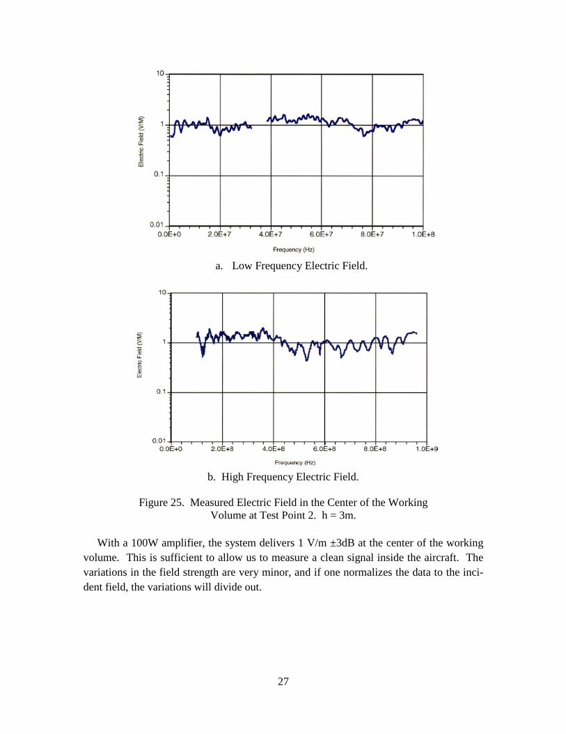
From this, we can get Einc by assuming the free space impedance Zo = 377Ω. However, since Ehorizontal goes to zero at a conducting interface (The ground is close to that.), we can’t measure E at that point. Instead, we measure it at some point above the ground where we will pick up both Einc and Ereflected. The measurement point is usually chosen to be the center of the working volume at the top of the aircraft fuselage. In this case, the measurements were taken at y = 3m. The measured electric field directly under the balun at a height of 3m above the ground is shown in Figure 25. (Note that there is a skip band between 320 and 380 MHz and another between 960 MHz and 1.0 GHz.)

27

a. Low Frequency Electric Field.

b. High Frequency Electric Field.

Figure 25. Measured Electric Field in the Center of the Working

Volume at Test Point 2. h = 3m. With a 100W amplifier, the system delivers 1 V/m ±3dB at the center of the working volume. This is sufficient to allow us to measure a clean signal inside the aircraft. The variations in the field strength are very minor, and if one normalizes the data to the inci-dent field, the variations will divide out.

28

Figure 26. Incident Magnetic Field (x 2) Measured on the Ground. 100kHz - 1GHz. Although the balun was designed to operate only up to 1 GHz, we ran it higher one day, just to see how it behaved. Figure 26 shows the measured data up to 3 GHz. Even with the variations, it is still usable up to about 2.5 GHz until the balun begins to reso-nate.

Figure 27. Electric Field Measured up to 3 GHz (TP 0,3,0).

In addition, measurements were made at 4 different locations within the working vol-ume that correspond to the nose, tail, and wingtips of an aircraft under test to get a meas-ure of the uniformity of the fields over the test object. These are shown in Figures 28 and 29 for the horizontal and vertical polarizations respectively.

29

Figure 28. Distribution of Simulator Fields in the Working Volume.

Horizontal Polarization.

Figure 29. Distribution of Simulator Fields in the Working Volume. Vertical Polarization.

10-1 100 101 102 10310-4

10-3

10-2

10-1 Horizontal Drive; Location 17

Fiel

d Re

spon

se (V

/m/V

)

Frequency(MHz)

10-1 100 101 102 10310-4

10-3

10-2

10-1 Horizontal Drive; Location 18

Fiel

d Re

spon

se (V

/m/V

)

Frequency(MHz)

10-1 100 101 102 10310-4

10-3

10-2

10-1 Horizontal Drive; Location 19

Fiel

d Re

spon

se (V

/m/V

)

Frequency(MHz)

10-1 100 101 102 10310-4

10-3

10-2

10-1 Horizontal Drive; Location 20

Fiel

d Re

spon

se (V

/m/V

)

Frequency(MHz)

10-1 100 101 102 10310-4

10-3

10-2

10-1 Horizontal Drive; Location 02

Fiel

d Re

spon

se (V

/m/V

)Frequency(MHz)

10-1 100 101 102 10310-4

10-3

10-2

10-1 Vertical Drive; Location 17

Fiel

d Re

spon

se (V

/m/V

)

Frequency(MHz)

10-1 100 101 102 10310-4

10-3

10-2

10-1 Vertical Drive; Location 18

Fiel

d Re

spon

se (V

/m/V

)

Frequency(MHz)

10-1 100 101 102 10310-4

10-3

10-2

10-1 Vertical Drive; Location 19

Fiel

d Re

spon

se (V

/m/V

)

Frequency(MHz)

10-1 100 101 102 10310-4

10-3

10-2

10-1 Vertical Drive; Location 20

Fiel

d Re

spon

se (V

/m/V

)

Frequency(MHz)

10-1 100 101 102 10310-4

10-3

10-2

10-1 Vertical Drive; Location 02

Fiel

d Re

spon

se (V

/m/V

)

Frequency(MHz)

30

10. Time-domain Analysis of Simulator Performance.

10.1. Impulse Response. Since the Ellipticus provides us with a stationary phase at the single radiating point and we have continuous phase across the entire spectrum, we can Fourier Transform the data to create a virtual impulse response. The resulting time-domain response is similar to what would be obtained from an impulse generator. One can trace the progression of the pulse from the network analyzer all the way through the coaxial cable and the balun to the measured fields underneath the antenna. Any imped-ance mismatches, reflections, or bad connectors show up readily and can be located from their time of arrival. Multiple reflections are easily noticed, and it is possible to relate the periodicity of the reflections to features in the frequency domain curves and vice versa. By looking at Fourier Transforms of the field measurements, especially the vertical fields, one can also assess the effect of any nearby structures. This is presented in detail in Appendix A. As has been stated before, now that we are testing at frequencies up to 1 GHz, we are seeing affects from things that we had never paid any attention to before, and the impulse response gives us a good tool to use to track them down. This process is described in much more detail in Appendix A. In Appendix A, the antenna was only swept to 100 MHz, so Dr. McLemore multiplied the waveform by a (sin x)/x function in order to shape the impulse. For the 1 GHz data, the impulse is very sharp, and we did not do that. The virtual impulses shown are simply from the Fourier Transform of the meas-ured field data.

10.2. Phase Slope and Time Delay. In Figure 30, we see the H-field measured in

the working volume and it’s Fourier Transform. As a sanity check, we can look at the phase shift and the time delay and see if they correlate with theory.

a. Magnitude.

31

b. Unwrapped Phase.

c. Impulse Response.

Figure 30. Phase Slope and Time Delay of a Measured Magnetic Field.

The phase slope is Δφ

Δω , where φ is in radians and ω in radians/sec. Therefore, the

phase slope is in units of seconds, and it should correspond to the time or arrival of the impulse. In this measurement,

Δφ = (2 x 105 deg) 2π radians360 degrees

= 3491 radians.

Δω = 2π · Δf = 2π x 109 radians/sec.

Therefore, Δφ

Δω = 550 ns (2)

which is exactly what we observe in Figure 30c.

32

11. Extrapolation to Criterion EMP. In order to extrapolate the data to a criterion EMP and/or compare it with measure-ments from ATHAMAS I, we must extract the reflected field in order to isolate Einc and Hinc. To do this we measure Etotal and Htotal at the same location in space, where

Etotal = Einc + Ereflected

(Note that Ereflected is negative.) Htotal = Hinc + H reflected

Then, Einc(ω) = ½ [ Etotal (ω) + Zo Htotal (ω) ] = ZoHinc(ω). (3) This is illustrated in Figure 24 above.

12. CW-to-Pulse Comparisons. Below are three examples comparing CW and pulse measurements made on three dif-ferent aircraft.

12.1. Example 1: EMPTAC Measurements. This shows a limited comparison between measurements made in the ATHAMAS II simulator and the Ellipticus CW illu-minator on the EMPTAC aircraft. Figures 31 and 32 are plotted on a linear scale, which emphasizes the peaks and suppresses the smaller parts of the data. Such a plot makes it easy to see how a strong fuselage resonance can affect the data when it is recorded on a digitizer with limited dynamic range. A plot on a log scale would emphasize the smaller data coming after the resonant peak. Some examples of this are shown in Figures 30 and following. Test Point 110Y was an unshielded cable bundle in the cockpit and TP 2142 was a common mode core current measurement made inside a shielded cable in the aft com-partment. In both cases, the CW data was extrapolated to the HPD radiated waveform for comparison. In these two figures, “measured” refers to the HPD measurement and “CW scaled” refers to the Ellipticus.

33

Figure 31. Ellipticus to HPD Comparison for Test Point 110Y.

Shown on linear scale.

Figure 32. Ellipticus to HPD Comparison for Test Point 2142.

Shown on linear scale.

12.2. Example 2: Other Aircraft Measurements. The data shown below was from a test on a similar military aircraft at Patuxent River NAS made within the last few years. In this data, we can see frequency, phase, as well as time domain comparisons be-tween the two simulators. In Figures 33 and 34 are some examples of CW and pulse measurements on cables inside an aircraft. Green = original HPD measurement before extrapolation. Blue = HPD measurement extrapolated to MIL-STD-464.8 Red = CW extrapolated to MIL-STD-464.

8 PST refers to the Passive Systems Test portion of the EMP test program. That is, transient EMP current measurements made on the aircraft with power off.

34

a. Time-domain comparison.

b. Frequency-domain comparison.

c. Unwrapped phase comparison.

Figure 33. Example of CW-to-Pulse Correlation of Aircraft

Cable Current Measurements.

We can see that the time-domain waveforms are not aligned in time, because the CW and Pulse measurements systems do not have the same time reference. The transient data begins when the pulser switch fires, whereas the CW data is referenced back to a sensor on the power amplifier. In this example, we have not attempted to align the data, but

35

have left them separated for clarity of viewing. If the peaks were aligned, one can see that the waveforms are very similar. The difference in the delay times is also evident as a shift in the phase slope as seen in Figure 33c. This data has been plotted on a log scale, so the phase appears as exponentially curved lines. If it were plotted on a linear scale, the phase would appear as an almost straight line, and the change in phase slope would be more obvious. This is further illustrated in the two examples below.

12.2.1. Phase Response and the Noise Floor. If we unwrap the phase data and create a continuous curve, we can also clearly see when the data system is approach-ing its noise floor. In Figure 33c, we see that around 250 MHz, the phase of the transient measurement begins to wander, a clear indication that the instrumentation system is oper-ating at the limit of its dynamic range. This then defines the noise floor. This is more clearly seen if the phase is plotted on a linear scale as seen in Figure 34. Another exam-ple is shown in Figure 35.

Figure 34. Unwrapped Phase of the Fourier Transform of a Pulse Measurement on a Cable. Linear scale.

Figure 35 below is an example of a cable current that is dominated by the aircraft fuselage resonance. As we can see, the frequency domain data is very noisy above about 10MHz, but it is almost impossible to determine exactly where the signal falls below the noise floor. By unwrapping the phase, however, we can see more clearly what is happen-ing. We see from the CW measurement that the measurement has higher frequency con-tent, but it is small compared to the dominant resonant peak at 3MHz. As a result, since the dynamic range of the transient instrumentation is only about 32dB, we can see that the phase begins to drop below that threshold at around 50MHz. On the other hand, the CW system, which has a dynamic range of 120dB, can continue to record signal. In these aircraft measurements in HPD, it was very handy to have the CW measurements to com-

36

pare to. This helped the data analysts a great deal to more clearly see where a given piece of data fell into the noise so they could apply a digital filter and get rid of it.

a. Extrapolated time-domain comparison.

b. Frequency-domain comparison.

c. Unwrapped phase comparison.

Figure 35. CW-to-Pulse Comparison of Aircraft Cable Current Measurements

with Strong Fuselage Resonant Coupling.

37

12.3. Example 3: Comparison of the Norms. In 2008, a comparison was made between CW and Pulse data taken on a small aircraft at Patuxent River. In Figure 36, we see the comparison between the three principal norms that are used in most EMP evalua-tions. (All were extrapolated to MIL-STD-464.)

Figure 36. Comparison of the Principal Norms in the CW and Pulse Measurements.

We see that for this data set, the average difference is no more than 3.4 dB, and the standard deviation is < 5 dB, which in our opinion indicates extremely good correlation! We notice the one oddball measurement in each of the three histograms. It turns out that this is the same test point in all three graphs. This leads us to be very suspicious of that measurement. It should have been double checked, but the data was not reduced until after the test, and the opportunity to correct it had passed.

12.4. Putting the CW Measurements in Perspective. The field radiated by the Ellipticus is spectrally flat across the entire measurement band. As a result, at the higher frequencies, the transfer functions Icable(ω)/Hinc(ω) will be exaggerated. However, when the data is multiplied by the EMP spectrum of Figure 1 during the extrapolation process (Equation 2), the high frequency responses will be greatly suppressed and no longer look out of proportion. For example, we can see in the CW leg current data of Figure 22b that the regular spacing of the ferrite beads (0.5m) causes notches at 250, 500, 750, and 1000MHz. This provides us with excellent diagnostic information, but after multiplica-tion by the EMP spectrum, the effect will be considerable suppressed. In general, we observe in the CW-to-pulse comparisons with ATHAMAS II that if there is a strong signal on the measured cable, the comparison is good. If the signal is weak, then the data is noisier, and the comparison is not as good.

a. Time-domain Peak b. Peak Rate of Rise c. Root Action Integral

38

13. Summary

If one wishes to compare low-level CW measurements with high level pulse, one must have the same field configuration and impedance in both facilities. Ellipticus provides a proper environment for estimating the coupling to the aircraft, for comparison to HPD and to evaluate the shielding elements on an aircraft. In the last 2 years, aircraft Swept CW testing capability has improved a great deal and now operates over the full range of HEMP frequencies in both horizontal and vertical po-larizations. While using this capability in this last year, we have gained some valuable insight into the proper methods of making HEMP measurements above 100MHz where wavelengths range from 3m at 100MHz to only 30cm at 1GHz. In the higher frequency regime, features of the simulator and instrumentation system that previously went unno-ticed suddenly become important. These include the length of the instrumentation cables, the spacing between the ferrites on the antenna, or the presence of small scattering ob-jects. We can also clearly see the high frequency losses in the concrete parking pad and ground plane mesh as a function of frequency, just as the theory predicts. These losses are present in the pulse measurements too, of course, but are more difficult to see because of the limitations of the transient recording system. Thus, having the CW capability pre-sent along with the EMP simulator will help identify areas where the facility design and the instrumentation design can be improved. We have learned the value of continuous, unwrapped phase data and how to use it and the impulse response as diagnostic tools. As a result, we see how valuable it is to have an antenna that operates continuously across the entire band. Note that the HPD and Ellipticus are designed to simulate the environment seen by an aircraft sitting on the ground only. To estimate the in-flight response requires a ground-to-air extrapolation procedure such as the “3C” procedure described by Baum [12]. However, it should be mentioned that for a small fighter aircraft, a very good in-flight simulation can be achieved by supporting the aircraft above the ground on a wooden test stand. The previous one used at Kirtland AFB was 10m high, but one could be made a bit smaller and still be effective. References 1. W.D. Prather, D.P. McLemore, et al, “Comparison of the Low Level Ellipticus and

High Level Pulse HPD Currents on the EMPTAC Aircraft,” IEEE Int’l Symposium on EMC, Dallas, August 1993.

2. Carl E. Baum, “Review of Hybrid and Equivalent Electric Dipole EMP Simula-tors,” Sensor and Simulation Note 277, Air Force Weapons Lab, Oct 1982.

39

3. W.D. Prather, “Elliptic CW Antenna Design,” Miscellaneous Simulator Memo 24, Air Force Weapons Laboratory, Kirtland AFB, NM, March 1987.

4. C.E. Baum, “Fields at the Center of a Full Circular TORUS and a Vertically Orient-ed TORUS on a Perfectly Conducting Earth,” SSN 160, Air Force Weapons Labor-atory, December 1972.

5. W.S. Kehrer, “ATHAMAS II Antenna Resistive Loading,” ATHAMAS Memo 7, Air Force Weapons Laboratory, July 1975.

6. T. Tran, R. Torres, W. Prather, D. McLemore, J. Martinez, and C. Zuffada, “Test Results for the Phillips Laboratory High Frequency CW Simulator,” HPM Confer-ence, August 1992.

7. C.E. Baum, W.D. Prather, and D.P. McLemore, “Topology for Transmitting Low-Level Signals from Ground Level to Antenna Excitation Position in Hybrid EMP Simulators,” Sensor & Simulation Note 333, AF Phillips Laboratory, Sept 1991.

8. G.D. Sower, D.P. McLemore, and W.D. Prather, “Ellipticus Ferrite/Resistive Load-ing,” Measurement Note 41, Air Force Phillips Laboratory, February 1993.

9. C.E. Baum, “Multiconductor-Transmission-Line Model of Balun and Inverter,” Measurement Note 42, Phillips Laboratory, 1 March 1993.

10. G.D. Sower, D.P. McLemore, and W.D. Prather, “Quad Coaxial Balun (QCB),” Measurement Note 44, August 1993.

11. G.D. Sower and L.M. Atchley, “Twin Coaxial Balun (TCB) Development,” Meas-urement Note 34, 3 June 1987.

12. C.E. Baum, “Extrapolation Techniques for Interpreting the Results of Tests in EMP Simulators in Terms of EMP Criteria,” Sensor & Simulation Note 222, Air Force Weapons Laboratory, Kirtland AFB NM, March 1977.

Additional Bibliography 13. C.D. Taylor, S. Langdon, and S.J. Gutierrez, “On the Wide-Band CW Illumination

of Large Scale Systems: The Ellipticus Illuminator,” IEEE Trans. On EMC, Vol. 37, No. 3, August 1995.

14. D.P. McLemore, et al., “The Phillips Laboratory Broad Band, HF CW Simulator,” National Radio Science (URSI) Meeting, Boulder CO, January 1993.

15. Y.G. Chen, R. Crumley, C.E. Baum, and D.V. Giri, “Field-Containing Inductors,” Sensor & Simulation Note 287, Air Force Weapons Laboratory, July 1985.

16. D.V. Giri, C.E. Baum, and D. Morton, “Field-Containing Solenoidal Inductors,” Sensor & Simulation Note 368, Air Force Phillips Laboratory, July 1994.

17. “Ellipticus CW Illuminator in Palmdale, California,” Final Report, DC-TR-5008.301-2, Kaman Sciences, March 1996.

18. Earl Dressel, et al., “Characterization of the Portable Ellipticus Antenna Simulator Modified to Allow Directional Illumination,” AMEREM ’96, Albuquerque NM, May 1996.

40

APPENDIX A

Time-Domain Analysis of the Ellipticus Simulator A.1. Introduction. This section was taken in large part from the Final Report for the Ellipticus at Palmdale CA [A-1]. It describes the technique used by Dr. Don McLemore to evaluate the performance of the original Ellipticus system which was swept from 100kHz to 100MHz. He measured the input current to the antenna as well as the fields in the working volume and transformed them into the time domain. The resulting time-domain response is similar to what would be obtained from an impulse generator. One can trace the progression of the pulse from the network analyzer all the way through the coaxial cable and the balun to the measured fields underneath the antenna. Any imped-ance mismatches, reflections, or bad connectors readily show up from their time of arri-val and the time of arrival of the reflection. Multiple reflections are easily noticed, and it is easy to relate the periodicity of the reflections to features in the frequency domain curves and vice versa. By looking at Fourier Transforms of the field measurements, one can also assess the effect of any nearby structures, wiring, or buried pipes. The data evaluation presented in this appendix addresses the antenna currents and the fields directly beneath the antenna apex. Section A.2 below first describes the data pro-cessing that was performed to calculate the time domain impulse response of the meas-urements. A.2. Time Domain Impulse Response. The time domain impulse response is obtained by taking the inverse Fourier transform of the corrected measurements. Since the meas-ured data are all normalized by the network analyzer drive voltage, the impulse response consists of the field or current that would result from a virtual impulse originating from the network analyzer at time t = 0. The virtual impulse would have a flat frequency spec-trum from 100kHz to 100MHz and a time domain waveshape of the general form:

𝑉(𝑡)𝑑𝑟𝑖𝑣𝑒 = 𝑉0 sin (𝜋∆𝑓𝑡)𝜋∆𝑓𝑡

(A-1)

where Δf = 100MHz and V0 is a constant. The zero-to-zero time duration of this impulse is 20ps. In order to perform an inverse Fourier transform on the corrected response data, the skip bands were first filled by inter-polation. The data was then interpolated again to provide digital files with 1024 sample points with uniform frequency spacing across the entire frequency range in order to be able to perform the Fourier transform. The phase data were unwrapped before interpolat-ing in order to prevent interpolation errors. An inverse FFT algorithm was used to obtain the impulse response of the fields and antenna currents.

41

A.3. Absolute Time Reference. All impulse responses have a common time reference defined to be zero when the virtual drive pulse is emitted by the network analyzer.9 The drive pulse propagates inside the coaxial cable to the antenna apex where it excited an-tenna currents and produces the illuminator fields. The data analysis that follows indi-cates that it takes 0.53μs to reach the antenna apex. Thus, all the field and current im-pulse responses occur after this point in time. A.4. Antenna Currents. Figure A-1 shows the antenna currents measured about 0.5m from the southeast (drive end) and northwest terminations. Below 5MHz, the data are almost the same, and above 5MHz, they exhibit similar overall frequency dependence. Both current measurements show an amplitude periodicity of about 1 to 3 MHz, which is associated with antenna resonant responses. This same resonance phenomenon can be seen from a time-domain perspective in the impulse response data shown in Figure A-2. In order to illustrate the time sequence of this response, the arrival time of the drive pulse at the antenna apex is denoted by a bar at t = 530ps. (This time identification was ob-tained from the field data discussed in Section 5.3 below.)

Figure A-1. Amplitude of Leg Current 0.5m from the Bottom on Both Ends.

A current pulse propagates from the apex down both antenna arms, arriving at each termination 210ps later at t = 740ps. Two additional small amplitude pulses are seen ar-riving at t = 1120 and 1760ps. The first small pulse is caused by reflection of the initial pulse at the termination and subsequent propagation back to the opposite termination. This corresponds to a total propagation distance of 115m, which is the combined length

9 The PHSTS van uses the output of the power amplifier as its phase reference instead of the network ana-lyzer.

42

of both antenna arms. The second small pulse is caused by an internal reflection of the drive pulse at the antenna balun at t = 530ps, propagation back through the coaxial drive cable to the amplifier, reflection from the amplifier back to the antenna apex, followed by current propagation along the outside of the antenna arms to the terminations. As was the case for the primary drive pulse, the time of arrival of the second drive pulse at the anten-na apex must be 200ps before a current is observed at the terminations. Therefore, it is designated by a bar in Figure A-2 at t = 1550ps. (This time of arrival is consistent with the length determined for the drive coax in Section A.6, i.e. 153m. Note in Figure A-2 that the time difference between the arrival of the second drive pulse and the primary pulse at the apex is 1550 - 530 = 1010ps. This corresponds to the electrical length be-tween the apex and the amplifier of 151.5m. The extra meter and a half between this length and 153m accounts for the coaxial cable from the network analyzer to the amplifi-er as shown in Figure A-1.) It is interesting to show how the two secondary current pulses at t = 1120ps and 1760ps effect the 1-3MHz periodicity seen in the frequency domain current response in Figure 20. This periodicity can be removed by first hand editing the impulse response data in Figure A-2 to eliminate the two secondary pulses (i.e. set the current after 1100ps to zero) and then taking the Fourier transform. The result is shown in Figure A-3 over-laid with the unedited data, which is the same as in Figure 20. Comparing these two plots clearly demonstrates that the two secondary pulses are responsible for the observed peri-odicity. Physically, the antenna current pulse at t = 1760ps could be removed if one could eliminate the reflection of the drive pulse at the balun or at the amplifier. The antenna current pulse at t = 1120ps is harder to eliminate, because it originates from the antenna current reflection at each termination. However, one might be able to reduce these reflec-tions with better impedance matching at the terminations.

43

Figure A-2. Antenna leg current impulse response 0.5m from southeast (drive) and northwest (termination) ends of the antenna, shown on two different time scales.

Figure A-3. Antenna leg current 0.5m from antenna southeast (driven) end,

with and without secondary reflections.

44

A.5. Reflections at the Termination. Additional information about the current reflec-tion at the termination is contained in the overall shapes of the two current pulses arriving at 740ps. These are illustrated on an expanded time scale in the lower portion of Figure A-2. Notice that the two pulse durations are in the 30-to-50ps range, which is about twice as long as the initial virtual impulse of Equation A-1, i.e. 20ps. The current pulses are broadened by propagation losses that increase with frequency, and because a slightly time-delayed reflected pulse is superimposed on each incident pulse. Since each current measurement was performed about 0.5m from the termination, it includes the incident pulse followed by a reflected pulse 3ps later. While the incident pulses at both termina-tions should be almost identical, the reflected pulses will be different because the termi-nation impedance is different at both ends. The antenna arm at the NW end, away from the drive, is terminated directly into a grounding rod, while the antenna arm at the SE end, the drive side, is terminated into a grounding rod in parallel with the drive cable, which is loaded with inductive chokes. Apparently this difference in the termination con-figurations changes the impedance and reflection coefficient enough to cause the ob-served difference in wave shape. This is manifest in the frequency domain data by the overall difference (ignoring the 1-3MHz periodicity) in the frequency dependence of the current, particularly above 5MHz. This small difference in the reflections at the two ter-minations produces a very slight asymmetry in the field responses in the plane of the an-tenna.

Figure A-4. Test point locations and field components measured at each location.

45

A.6. Fields Directly Beneath the Apex. Horizontal Polarization. A.6.1. Magnetic Field On the Ground Plane. Figures A-5 and A-6 show the

principal field components, Hz and Ex, measured directly beneath the apex of the antenna. Since Hz adds constructively on reflection from the ground, the reflected Hz field at Test Point 1 has the same wave shape and frequency spectrum as the incident field. Thus, the measured field (total field) at this location has the same frequency dependence, but about twice the amplitude of the incident field alone.

Figure A-5. Amplitude of the Principal Magnetic Field Component, Hz, at TP 1 and 2.

TP 1 is on the ground. TP 2 is 3m up.

Figure A-6. Amplitude of the Principal Electric Field Component, Hz, at TP 2.

46

Figure A-7 shows the impulse response of the total Hz field on the ground plane at TP 1. Note that the virtual impulse arrives at TP 1 at t = 610ps. Since the antenna apex is 25m above the ground, the virtual impulse must have begun propagating from there at t = 530ps, as previously noted.

Figure A-7. Impulse Response of Hz at Test Point 1.

The electrical length of the drive coax from the network analyzer to the apex is obtained by multiplying the transit time by the speed of light to get 153m. This includes the length of one antenna arm. One would expect the incident field at TP1 to have the same general wave shape as the virtual impulse of Equation A-1, and this is indeed the case before the pulse reaches its peak value. After the peak, however, the field oscillations appear to be inconsistent with the drive waveshape. The most probable explanation for this is that the balun at the apex is not working properly because of damage or incorrect installation. This could also explain why there is such a strong reflection inside the drive coax at the antenna apex. The only alternative explanation for the field oscillations immediately after the peak of the pulse would be scattering from the antenna arms. A.6.2. Fields at 3m above the Ground Plane. Figures A-5 and A-6 show the frequency domain response of Hz and Ex at TP2, which is 3m above the ground, directly beneath the apex. Figure A-8 shows the corresponding impulse responses. It should be noted that all the H-field impulse responses in this appendix have been multiplied by 377Ω so they will have the same normalized units as the E field. Once can see by the overlay of the incident E and H fields that their ratio is 377. One can also see that the E field in Figure A-8 has a negative spike about 20ps after the main pulse caused by the reflection from the ground. The H field has a positive spike since it reflects in phase. (Recall that the incident field also has a positive spike at 20ps after the initial pulse (see Figure A-7), which attributed to the balun. In Figure A-8, the ground reflection adds to the spike in the incident H field and subtracts from the spike in the incident E field.

47

Figure A-8. Impulse Response of Ex and Hz at Test Point 2.

A.6.3. Extracting the Incident Field. In order to support the above interpreta-tion of the impulse response data, it is useful to obtain an independent estimate of the in-cident field from the data at TP2. This can be done by adding Ex to 377 x Hy. Figure A-9 shows the result along with the Hz field at TP1.

Figure A-9. Synthesized Incident Field at Test Point 2 Compared to the Measured

Magnetic Field at Test Point 1.

48

The field strength for the synthesized incident field at TP2 was reduced by the ratio of the distanced from the apex to TP2 over the distance to TP1 (i.e. 22m/25m) to account for the 1/r fall-off due to the additional 3m of propagation. This scaling is only approximate and is intended only for easier visual comparison between the data from the two test points. It is clear from Figure A-9 that, except for the amplitude and time of arrival, the two inci-dent wave shapes are the same. A.6.4. Fields from the Secondary Pulse. The secondary pulse identified from the antenna leg current data discussed in Section A.1 above occurs at t = 1550ps and is also apparent in the field data. Recall that the original drive pulse is reflected from the antenna apex at t = 530ps, propagated back to the amplifier and reflected back to the apex to excite once again the antenna gap as a secondary pulse at t = 1550ps. This pulse can be seen in the time domain field of Figure A-7 at t = 1600ps and in the fields of Figures A-8 and A-9 at t = 1620ps. It can be seen more clearly on the smaller amplitude scale and shifted time window in the lower part of Figure A-9. Note that both plots in Figure A-9 display the same data, only scaled and plotted differently. Comparing the wave shapes in the upper and lower plots, one can see that they are not identical, but neverthe-less very similar. The reason they are not identical is because the secondary pulse is dis-torted by the reflections at the apex and amplifier and by attenuation caused by the triple-pass propagation through the drive coax. However, the overall features of the secondary pulse are unmistakably similar to the original pulse. In fact, the secondary pulse was ob-served in the impulse responses of all the measured data that was processed in this way, and its waveshape always had the same general features as the primary pulse.

A.6.5. Possible Improvements. The periodic variation in the frequency domain data are caused by 3 physical effects: 1) reflection from the ground, 2) reflection and scattering from the antenna terminations, and 3) the secondary pulse. It is possible, of course, to suppress the appearance of the scattered pulses in the time domain data of Fig-ures A-8 and A-9 by hand editing out (time gating) the secondary pulses and setting the response to zero after t ≈ 900ps. This allows a better look at the behavior of the antenna and balun without these pulses. However, the secondary reflections are actually there in the transmitted waveform and so must be left in when the antenna is used to measure an aircraft unless they could be edited out in both the incident field waveform and the meas-ured aircraft waveform. Figures A-10 to A-12 show the changes in the frequency domain data after the im-pulse responses have been edited and Fourier transformed. Notice that much of the peri-odicity has been removed, attesting to the fact that the periodicity was in fact caused by these secondary pulses. The remaining periodicity in Figure A-10 results from the de-graded balun performance or possible scattering from the antenna arms. Normally one would expect the balun response to be smooth and flat as a function of frequency. How-ever, based on the data in Figure A-12, the balun or the antenna arms seem to have sever-

49

al strong resonances, particularly around 13MHz. In addition, there is a periodicity of about 50MHz associated with reflections over an electrical length of about 3m. This is the cause of the spike in the impulse response of the incident field that occurs 20ps after the primary impulse.

Figure A-10. Amplitude of Hz at TP2, With and Without Hand Editing to Remove the Effects of Scattering From Terminations and Secondary Pulse at t = 15550ps.

Figure A-11. Amplitude of Ex at TP 2, with and without Hand Editing to Remove the Effects of Scattering from Terminations and Secondary Pulse at t = 1550ps.

50

Figure A-12. Amplitude of Hz at TP 1, With and Without Hand Editing to Remove the Effects of Scattering from Terminations and Secondary Pulse at t = 1550ps.

References A-1. “Ellipticus CW Illuminator in Palmdale, California,” Final Report, DC-TR-5008.301-2, Kaman Sciences, March 1996.