Embed Size (px)
Citation preview

I
Sensor and Simulation NotesNote 147
-’
(Radiation Laboratory Report
March 1972
MODIFIED BICONICAL .
No. O1O748-1-T)
T. B.A. Senior and G.A. Desjardins
The University of Michigan Radiation LaboratoryDepartment of Electrical Engineering
Ann Arbor, Michigan
Abstract
48105
The early time behavior of the fields radiated by two types of EMPantennas is investigated. The first type is a bicone-cylinder in which each coneis mated directly to a semi-infinite cylinder of constant radius, thereby creatinga ring discontinuity in slope at the junction. The second assumes a continuationof the bicone which matches the slcpe at the junction with the cone, producingthere a ring discontinuity in curvature. Using geometrical diffraction theorytechniques and knowing the diffraction matrices for the hvo forms of surticesingularity, a high frequency asymptotic development of the radiated field isobtained for each autenna. Application of an inverse Fourier transform thenyields a time domain solution valid for sufficiently early times. The solutionsare computed and their validity investigated. Examples are given showing thereduction in the perturbation of the early time response associated with thesmoother geometry.
,..
.-
-. —.. . .. . . . . . -,. .._ , .— —----
—.- .-. .- — s.--..—. — . _ . .. . .. .._ Q..4?/ikllqt~(

..
●
b
1. Introduction
● From an electromagnetic viewpoint the infinite biconical antenna is an
. ideal device for radiating an EMP. Since a constant voltage applied across the
infinitesimal gap separating the two halves of the bicone produces a pure frequency-
independent spherical TEM wave, a voltage pulse will create a radiating pulse
which is identical in all respects. Unfortunately, such an antenna is unrealistic
because of its infinite dimensions parallel and perpendicular to the axis of
symmetry. A compromise which seeks to retain some of the electromagnetic
advantages of the bicone whilst making the transverse dimensions finite is to mate
each half of the bicone to some other geometrical structure at a selected distance
from the gap. By choosing this structure to be a semi-infinite circular cylinder,
we arrive at the bicone-cylinder studied by Sancer and Varvatsis ( 1971) and char-
acterized by a slope discontinuity at the join. Within the spatial region which is
directly illuminated, it is expected that the dominant contribution will still be the
undistorted pulse radiated by the gap, but because of diffraction at the joins and
*the multiple interactions of these diffracted pulses with the rest of the antenna,
the net field will be affected, with the short time perturbations being attributable
to the diffraction of the high frequent y components. Any modification in the
cylindrical structure beyond the join will have a dominant effect on the field with-
in the shadowed region which is entirely diffractive in nature, and can also distort
yet further the field in the illuminated region through back reflection. On the semi-
infinite cylinder, however, the surface field is primarily a traveling or surface
wave excited by the join. If this were attenuated by progressive loading of the sur -
face, the cylinder could then be terminated without further affect on the field in the
illuminated region. Only on such a premise would an exact analysis of an infinite
bicone-cylinder be relevant to a realistic antenna, and we must emphasize that the
relevance would not extend to the deep shadowed regions of space.
The right circular cylinder is only one type of continuation structure for.
the bicone, and an infinity of other continuations are possible which also serve to
limit the transverse dimension of the resulting antenna. One class of these produces
O.-1

.,
b
*
a smoother transition between the bicone and the continuation by matching the
slope whilst leaving the curvature discontinuous at the join, and still higher order
matching could be entertained. Such smoothing of a surface singularity reduces
the high frequency diffraction, implying that a change from a slope discontinuity
(in the first derivative of the profile) to a curvature discontinuity (in the second
derivative of the profiie) will decrease the perturbation of the direct radiated
pulse for at least some span of elapsed time.,<
Since the precise leading term in
a high frequent y asymptotic expansion of the diffraction coefficient for a line dis -
continuity in curvature has recently been obtained (Senior, 1971), it is now pos-
sible to quantify this effect. This is the purpose of the present Note.
We here examine the consequences as regards the early time behavior of
the radiated field of replacing a cylindrical continuation of the bicone by a hyper -
bolic continuation ‘so chosen as to remove the discontinuity in slope at the junction.
The procedure that is adopted is to calculate the leading (first order) term in the
high frequency expansion of the diffracted field at any arbitrary point in the illu-
minated region for each of the two geometries. The time domain solution for a
step function voltage applied across the gap is then obtained by an inverse Four-
ier transformation. Although the range of elapsed times for which this so~ution
is valid cannot be stated with any real certainty, an upper bound is available from
a consideration of those ray interactions which are ignored in the frequency domain
analysis. Not surprisingly, at every point in spac,e there is some range of
elapsed time for which the perturbation of the undistorted pulse is smaller when
the discontinuity y is in curvature rather than slope. Data are presented illustra-
ting this effect and some general conclusions are drawn, but whether the improvem-
ent is sufficient to outweigh the disadvantages of this new geometry is a question
beyond the scope of this Note.
These disadvantages are two-fold: increased difficulty of construction to
produce the smooth junction and an increase in the overaH diameter of the antenna.
For any smooth and monotonic continuation, the maximum radius necessarily y ex-
ceeds the radius of”the join, and for the hyperbolic profile assumed in the analy-
sis, the discontinuity in radius of curvature is proportional to the fractional
2
.
6
* increase in maximum radius on changing from a cylindrical continuation (slope
discontinuity). Indeed, this fractional increase is one of the key parameters in
the final presentation of our results, but in practice it should be possible to ob-
tain the advantages of the smoother geometry with a smaller increase. The only
portion of the continuation structure which is essential to the analysis is that
which is just beyond the join. The surface field here is basically a creeping
wave whose strength and attenuation are known (Weston, 1965; Hong and Weston,
1966) . Because of this attenuation, the requirements on loading to permit ulti -
mate termination will be less stringent than was the case for a cylindrical con-
tinuation, and at some point of the curved surface beyond the join it would be‘.,
acceptable to change to another surface profile more nearly approximating that
of a right circular cylinder. The hyperbolic geometry would then apply only to
a transition region behveen the bicone and the structure further out, and provided
the second surface discontinuity was well within the shadow, its presence should
have no effect on the field within the illuminated region, certainly as regards the
early time behavior. However, these are practical considerations which are
irrelevant to the main thrust of our analysis.

2. Preliminary Considerations
.!
2.1 The Infinite Biconical Antenna
The antennas to be expiored are all geometrical modifications of the
infinite biconical antenna and it is therefore appropriate to consider first the
field radiated by such an antenna when excited by a point generator at the apex
of the cones,
The geometry is now as shown in Fig. 1. If (r, O, @)are sphericai polar
coordinates referred to an orgin at the apex, the field radiated by a time har-
monic voltage generator of circular frequency u = kc is
A(w) eik(r - et)~=&—— l!= ? * eit<(r-et)r sin (3 9
in which
(1)
A(w) = : 1(u, O)
where Z = l/Y is the intrinsic impedance of free space and 1(u, O) is the total
surface current entering the upper cone from the generator at r = O.
Knowing the structure of the field, we can integrate E. along the field
line r = constant, $1= constant from the va~ue @= 00 appropriate to the upper
cone to the value i3 = r -60 at the lower cone to obtain
V(W,r) = I(w, r) Zc
where
is the characteristic impedance of the antenna. In particular, at r = O
v(u) = r(u, o) zc
where V(u) = V(u, O) is the strength of the voltage source, and if we now write
4

z
●
\I /
\ I/
I/
\ M’
point genera
/I
/ I \
FIG. 1: INFINITE BICONICAL ANTENNA.

.
we have
(2)
a
A(u) = V(u)fo .
Tbe radiation field(l) is independent of @ andentirely specified by the 6
component of the electric field, viz.
‘(w)fO ik(r-et)‘6 =
—er sin 19
. (4)
Moreover, it is a function of frequency only through the phase factor and the
frequency dependence of the excitation voltage. It therefore foUows that if the
excitation is the voltage pulse v(t), it will
amplitude scaling factor fo/(r sin(3), and in
Heaviside) step function U(t), then
P
radiate undistorted except for the
particular, if v(t) is the unit (or
‘0‘e =
— U(t - :) ~r sine
(5)
We shalt henceforth restrict ourselves to such a voltage pulse.
2.2
For
Fourier Transform Relations
the modified antenna geometries discussed in Section 2.3 the pro-
cedure that we shall follow is to develop first a high frequency asymptotic
expansion of the radiated field for a simple harmonic source at the aWx of the
cones. In the illuminated region the leading term in the expansion is the field
(4) appropriate to an infinite biconical antenna. The higher order terms are
attributable to diffraction at the surface singularities, and to the accuracy that
this expansion can be found, these terms are of the form
1
V(w)w‘n- ~eik(t -et)
6
.
*
.- ●
for n = O, 1, where 1 is some distance, The early time behavior of the radiated
field is then obtained by appiying an inverse Fourier transform to each individual
term with V(w) as the spectrum of the unit step source voltage,
To permit the rigorous Fourier transformation of functions f{t) which do
not tend to zero as t + m, it is necessary to assume that w has a small positive
imaginary part c, With this extended definition, the Fourier transform of f(t) is
\
m
J {f(t)] = F(w) = e ‘Wt f(t) dt
J-a)
and the inverse transform is
(6)
(7)
J-m+ i~
If f(t) is tie unit step function U(t), direct integration shows that
F(u) = i/w .
Moreover, 3-1 {F(w)} can now be evaluated unambiguously, implying
u(t) = & ) -iwt‘e, dw. (8)w
-m + i~
Consider ~ -’{Q-’/21 where the cut originating at the branch point
w = O is assumed to lie along the negative real w axis. If t <0, the path of
integration can be closed by the addition of a semi-circle of large radius in the
upper half u plane and the transform shown equal to zero. If t >0, the addition
of a semi-circle in the lower half plane reduces the transform to the sum of
integrals along both sides of the cut, and these can be evaluated trivially. Hence
7

Integration by parts now yields the two results which are needed in the sequel,
viz.
(9)
and
3-1{iu-5/2 ~ikl
1=-
+ei”’4(’-:Y’2@ ~ “0)
which are special cases of the general formula
(11)
valid for positive integer n.
2.3 Specific Geometry
In the region adjacent to the gap the antenna is assumed to be a bicone of
half-cone angle 190, extending out to a radius d sin 13~ where d is the slant length
of the cone. At this point the profile is changed, and if p, z are cylindrical co-
ordinates with origin at the gap and z axis coincident
the requirements on the new profile p = P(z) are that
function of z with p + finite limit as z + m and
P = dsin607
go .) at z = dcos80 .=tane ~
with the axis of symmetry,
it be an analytic, monotonic
Since the entire configuration is symmetrical about the plane
cient to consider only the upper cone and its continuation.
The most simple function having the above properties
we therefore choose’ the hyperbolic profile
Z = O, it is suffi -
is a hyperbola, and
●. .
8

*
{- 1p-dsin OO=Btan60 1- ~ ~co~~ ~B ,0
for z~dcoseo, where B is some constant yet to be chosen. At the junction
with the upper cone, p = d sin 60 and dp/dz = taneo, as required, and the
(inward) curvature in any plane containing the z axis is
k sin 260COS6al=B 0“
This is the quantity which determines the strength of the field diffracted at the
junction of the bicone and its continuation.‘.
It only remains to express “B in terms of a convenient geometrical quantity
natural to the problem. For this purpose, we note that as z -+m,
p +dsin OO+Btan~O. Let us therefore write
Iim p = d(l+e)sin@o
2+0
where e is the fractional increase in the overail radius of the antenna on
from a circular cylindrical continuation of the bicone to a slope matching
Then
B = edcoseo
and
A sin 20al = cd o
with c = O implying a slope discontinuity at the junction.
(13)
changing
one.
(14)
. .
..*
.
3. Ray Techniques
The procedure that we shall follow in analyzing the transient radiation
from the antenna is to first develop a high frequency asymptotic expansion for
the field radiated when the voltage across the gap is a simpLe harmonic one with-iut
time variation e . The only effective method for doing so is to use the geo -
metrical theory of diffraction (GTD) originated by Keller (1957, 1962). The
theory is basically an extension of geometrical optics to include the concept of
diffracted rays produced by surface singularities, and since we shall re -phrase
slightIy the formulae of GTI) to emphasize still more the similarity to geometrical
optics, it is convenient to begin with a generaI survey of such aspects of ray tech-
niques as are appropriate to a problem such as this.
3.1 An Overview
In geometrical optics the propagation of energy between two points Q and
P occurs according to Fermat’s principle that the optical distance between Q
and P must be stationary with respect to small variations in path. In particular, a
therefore, the optical rays in a homogeneous isotropic medium are straight lines,
The variation of intensity of the geometrica~ optics field along a ray is dictated
by energy conservation: the energy flux in a tube of rays must be the same at all
points along the tube.
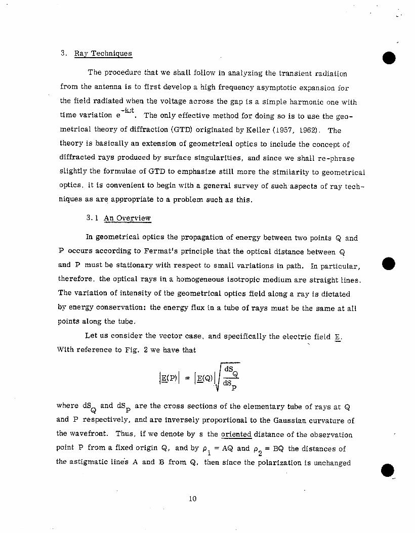
Let us consider the vector case, and specifically the electric field ~.
With reference to Fig. 2 we have that.
where dS and dSp are the cross sections of the elementary tube of rays at QQ
and P respectively, and are inversely proportional to the Gaussian curvature of
the wavefront. Thus, if we denote by s the oriented distance of the observation
point P from a fixed origin Q, and by pl = AQ and p2 = BQ the dis~nces of
the astigmatic line-s A and B from Q, then since the polarization is unchanged
Q
10

.-
dSQ /
dSP
FIG. 2: ASTIGMATIC TUBE OF RAYS.
- ,.. ,. ●,,1
.

--
along the ray,
&(P) = EJ(Q) ~eik(s -et)
where
r=
is the so-called divergence
/--
factor which isa measure of the spreading of the
(16)
elementary tube of rays from Q to P.
Equation ( 15) yields an infinite value for the fieid at the caustics A and
B where either s = -91 or s = -P2, implying r = m. This is a universal
failure of any ray technique and a procedure for obtaining a finite, frequency-
dependent expression for the field in the vicinity of a caustic has been discussed
by Kay and Keller ( 1954). However, on following a ray through a caustic and
beyond, r is again finite, and provided we interpret r -1 as -i, Eq. (16)
does predict the known phase delay of ~/2 on passing through a line caustic in
a positive direction.
At the surface of a body or, indeed, at any surface of discontinuity in a
medium, the direction and wavefront curvature associated with any ray change
discontinuously, as do the field strength and polarization. There are now two
distinct cases depending on the principal radii of curvature of the surface at the
point Q where the incident ray strikes. If both radii are non zero then, in the
high frequency limit, the incident ray will produce a single reflected ray whose
orientation is in accordance with Snell~s laws of reflection at a pLane interface.
This is the geometrical optics situation and the strength of the refiected field at
the surface is specified by the Fresnel reflection coefficients for plane wave
incidence on a plane interface. A general expression for Er(Q) has been derived—
by Fock ( 1965), and can be written most compactly as
E_r(Q) = ii* ~i(Q)
12

e
where the tensor reflection coefficient ~ is a function of the angle of incidence
and the electromagnetic parameters of the surface. For a perfectly conducting
body, ~ is such that fi~ ~r = -a ~ Jr
and $sIJ =fi”ql, where ?? is a unit vector
normal.
To calculate the field on the reflected ray at a point P which is away from
the surface we can again use Eq. ( i5) where p ~ and p2 are now the principal
radii of curvature of the reflected wavefront at the point of reflection, Q. In
general, these depend on the angle of incidence, LY, measured with respect to
the local normal, the radii of curvature, s ~ and S2, of the incident wavefront
at Q, measured in and perpendicular to the plane of incidence respectively, and
the corresponding radii, rl and r2, of the surface at Q. As shown by Fock
( 1965) and Senior ( 1972),
1 _+2seca _=~+2cosa1 1—= ,‘1 ‘1 ‘1 P2 %2 ra “
(18)
Observe that s ~, S2 and r , r are not necessarily principal radii of curvature.12
Indeed, if s ~ and s; are the principal radii for the incident wave front at Q and ~
is the angle between the plane of s f and the plane of incidence,1
(19)
and a similar pair of formulae hold for the surface curvatures.
The second case to be considered is that in which one or both of the
principal radii of curvature are zero at the point Q, corresponding to a line or
point (vertex) singularity respectively. Although geometrical optics is no longer
applicable, geometrical diffraction theory now takes over, and each incident ray
produces an infinity of diffracted rays. For the purposes of the present problem,
only the line singularity is important. This may be produced by a discontinuity
in the first derivative of the surface (wedge-like singularity) or in some higher
derivative, the earlier ones being continuous at Q, but in either case the diffracted
13

.-
.
rays are confined to the surface of the Keller cone. In the immediate vicinity
of Q the field on any one diffracted ray is entirely a local property of the sur - a“
face at Q, and can be found by soiving a canonical problem displaying the
geometry in question. In principal at least, this enables us to relate the
reflected field strength at a point close to Q to the incident field strength via
an equation similar to (17) in which a tensor diffraction coefficient takes the
place of F.
Unfortunately we now run into a conceptual difficulty in trying to find the
diffracted field at a remote point P along a diffracted ray. Since the surface
s insularity is a caustic for the diffracted ray tube in a plane perpendicular to
the singularity, we cannot use the divergence factor (16) to proceed outwards
from Q. For this reason, it has become customary (following Keller, 1957)
to omit any explicit statement of a diffraction tensor for points close to Q, and
to proceed immediately to a “remote” point P distance s (>> k) from Q, writing
the diffracted field there as
r‘1 ei7r/4 .
Ed(P) =\ ~1+5m ‘ll’(S ‘Ct) ‘“Ei(Q)
(20)
where pl is the transverse radius of curvature of the diffracted ray tube at Q.
If ~ is the angle between the incident unit vector ~ and a tangent unit vector ?
along the singularity or “edge’~r the local radius of,which is r ~, 7 is arclength
along the edge, 3 is the principal unit vector normal to the edge (i.e. pointing
towards the center of curvature) and ~ is a unit vector in the direction of the
diffracted ray, then
(21)
For a wedge-type singularity .
3= -cosec ~ T (22)
where ~ is given by Senior and Uslenghi (i971) in terms of a set of surface- 0--oriented base vectors.
14

Even if we grant that the above procedure is the most rigorously
justifiable ..one, we can still enhance the similarity of the diffraction and reilec -
tion processes by regarding ~ as a diffraction tensor which relates the field on
a diffracted ray at a distance s 21 from Q to the incident field at ‘Q. If this
displaced point is denoted by Q’, Eq. (20) can be decomposed into two equations
analogous to (15) and
where the divergence
and the proviso that
and though
for ks >> 1
deduced),
Eqs. (23)
( 17), viz.
~d(Q’) = ~ o~i(Q) , (23)
gd(P) = lJd(Q’) ~eik(s -et)
factor r has the standard form ( 16) with
P2=~
c i7r/4i=e . Thus
(24)
(25)
(26)
, (24) and (26) are no longer equivalent to (20) for ks & 1,
(the condition under which the diffraction tensor ~ was originally
(27)
and the equivalence is restored.
In a problem where both diffraction and reflection occur, the main
advantage of the present interpretation is that we can treat the two processes
similarly and proceed stepwise along all rays using the same general formula
for i’ . But the advantages are not overwhelming, and one penalty that we do
pay is that ~ can now involve the wave number, k.
15

3, 2 Diffraction Tensors.
The diffraction tensor for a line discontinuity in slope (wedge-like
singularity) was originally deveioped by Keller ( L957) and was put into a some-
what more general form by Senior and Uslenghi ( 1971). The analogous resuR for
a line discontinuity in curvature was obtained by Senior ( 1971), and to present,
the tensors in the form impkied by our preceding remarks, it is sufficient to
take “only a discontinuity in slope since the result for a discontinuity in curvature
differs only in the replacement of one pair of parameters by another.
Consider a wedge-like singularity shown in Fig. 3. Let the interior
half angle of the wedge be f2 and choose a base set of unit vectors f?’,I?,; withA AN normal to the edge and pointing out, B binormal to the edge and pointing
into the shadowed half space, and ; = R A~ to make the system right-handed.
Then if the incident ray direction is
(28)
with -~/2+ f2<cY<7r/2j O < P < ~ and the diffracted ray direction is
o~= ?cos P+ fisin6sin’Y -8sin Bcos T (29)
with -7T/2+f2<Y < 3m/2 -Cl (see Fig. 3), we have
(30)
.
at any point P of the singularity y where ~d(P) and ‘?_l(P) are the diffracted and
incident electric fields at P expressed as row and column vectors respectively
in the base ?, fi,fi, and
[
-(X-Y} o 0
~=-A (X-y) cot@sin7 (X+ Y)cos’Ycosa (X+ Y)cos?’sinf.Ysin P
-(X- Y)cot~cos? (X+ Y)sin7cosa (X+ Y)sinysind ,)
(Senior and Uslenghi, 1971, Appendix, with 6 = O) where -
a..

FIG. 3: GEOMETRY FOR A WEDGE-LIKE SINGULARITY,
*
with
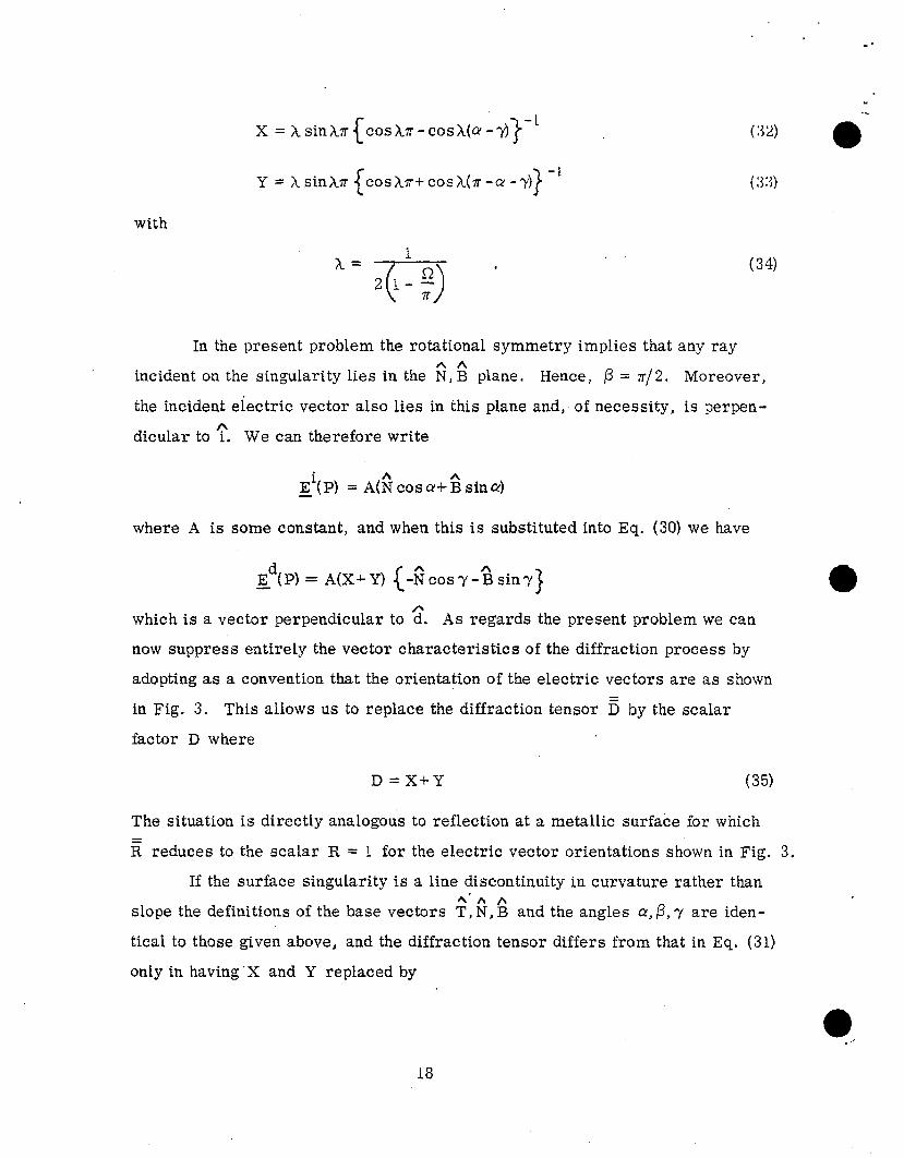
X = ksink7f{cos h.r-cos JJ~-y)}-i
Y = ksink7r {cosk7f+cosk(r -Q-y)] ‘i
.--
( 32) a(3:;)
(34)
In the present problem the rotational symmetry irnpiies that any ray
incident on the singularity lies in the 8, 8 plane. Hence, ~ = r/2. Moreover,
the incident electric vector also lies in this plane and, ~of necessity, is perpen-
dicular to ?. We can therefore write
where A is some constant, and when this is substituted into Eq. (30) we have
which is a vector perpendicular to ~. As regards the present problem we can
now suppress entirely the vector characteristics of the diffraction process by
adopting as a convention that the orientation of the electric vectors are as s hewn
in Fig. 3. This allows us to replace the diffraction tensor ~ by the scalar
factor D where
13=X+Y (35)
The situation is directly analogous to reflection at a metallic surface for which
~ reduces to the scalar R = 1 for the electric vector orientations shown in Fig. 3.
If the surface singularity is a Iine discontinuity in curvature rather than,
slope the definitions of the base vectors ?,;, 6 and the angles a, ~, Y are iden-
tical to those given above, and the diffraction tensor differs from that in Eq. (31)
only in having” X and Y replaced by
. .
●
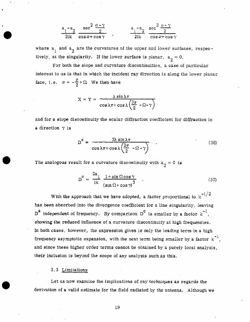
where a1
tively, at
s# ~al-a2 2
2ik cosa+cos’y ‘al-a2
2ik
and a2 are the curvatures of the upper
the singularity. If the lower surface is
~ec2 Q’+-i2—
Cos Q’+Cos -y
and lower surfaces, respec -
planar, an = O,
For both the slope and curvature discontinuities, a case of particular
interest to us is that in which the incident ray direction is along the lower pLanar
face, i.e. CY= -~ + Cl We then have
X=Y=ksinkr
(
3Tcos A7r+cos A ~ -WY
and for a slow discontinuity the scalar diffraction coefficient for diffraction in
a direction ? is
Ds =
The analogous result for
Dc =
a curvature discontinuity with an = O is
2a ~
:1>lJS
With the approach that
l+sinfi?cos~Q
(sin Q+cos y)”
we have adopted,
(36)
&
(37)
-1/2a factor proportional to k
has been absorbed into the divergence coefficient for a line singularity, leaving
Ds independent of frequency.-1
By comparison Dc is smaller by a factor k ,
showing the reduced influence of a curvature discontinuity at high frequencies.
In both cases, however, the expression given is only the leading term in a high
frequency asymptotic expansion, with the next term being smaller by a factor k ,-1
and since these higher order terms cannot be obtained by a purely local analysis,
their inclusion is beyond the scope of any analysis such as this.
3.3 Limitations
Let us now examine the implications of ray techniques as regards the
derivation of a valid estimate for the field radiated by the antenna. Although we
.“
shall obtain the time domain solution by inverse Fourier transformation of the.
high frequency response, quite different factors influence the accuracies in the m
two domains.
In the frequent y domain, the relative importance of individual contributions
to the field is determined by the k dependence of their amplitudes. If the ampli -
tude of a direct ray contribution from the source is A, where A is independent
of k, that for a contribution singly diffracted at a slope discontinuity is
Ak-’/2{l+0()}’)} . If a diffracted ray is subsequently reflected at a surface
whose radii are large, the k dependence is unaffected, though it should be noted
that the reflection coefficient is independent of k only to the leading order, On
the other ha~d, a secondary diffraction at a slope discontinuity will reduce the.
ampIitude to Ak-l {1 + O(k-l)] .
In the present problem it is possible for a ray to be diffracted bat!< to the
source and then re-radiated. It is intuitively obvious that the nature of this re -
radiation (or re -diffraction) will depend on the impedance of the source as well
as the geometry of the gap, but the factor which quantifies this process is quite
unimown even in its k dependence. It is therefore necessary to exclude any such a
ray contribution from our analysis, and the consequences of this are unfortunate.
at least from a rigorous viewpoint. If, for example, the factor were independent
of k, the contribution of a re-radiated ray would be of the same order as that for
a ray diffracted at a surface singularity y, regardless of its nature, and this would.-
invalidate all terms in the high frequency expansion beyond the first, corres pending
to direct radiation from the source; it is not inconceivable that the factor could be1/2
proportional to k , which would invalidate even the leading term !
The validity of even a single term in the high frequency expansion of the
field now rests on an assumption about the frequency dependence of the re -radia-
tion factor. On the premise that any EMP antenna which did not produce an early
time behavior of the radiated field comparable to that of the excitatiori voltage
would have its gap configuration changed until it did, we shall henceforth assume
that the re-radiation factor is proportional to some negative (perhaps fractional)
20

power of k, thereby reducing the importxmce of any such ray contribution below
that of a single diffracted ray, but not below that of a double diffracted ray, ‘f’ In
consequence, the only contributions which can be entertained are those of the
direct ray from the source and the rays singly diffracted at the surface disc on -
tinuities, either directly to the point of observation, or via an intermediate
reflection off the sides of the bicone. The resulting expansion in the frequency
domain is then
A+Bk ‘1/2{ l+ O(k-e)}
for a slope discontinuity, or
A+ Bk-3/2{J+0(k+)}
for a curvature discontinuity, where c >0 and we have again omitted the phase
factors produced by the different ray paths.
Let us now turn to the time domain. From a high frequency estimate of
the field we can deduce the early time behavior of the transient response by in-
verse Fourier transformation, but the validity of the result is not without question.
Whereas the lengths of the individual paths by which the ray contributions reach the
field point are no direct concern in the frequency domain, they are vital in the
time domain since these are reflected in time separations. The shortest ray
path whose contribution is omitted now provides an upper bound on the elapsed
time beyond which the time domain response is patently invalid. In the present
problem the bound is provided by either the doubly diffracted ray or the re -radiated
one, whichever is shorter, but even within this bound the accuracy of the solution is
not entirely certain. Take, for example, a singly diffracted ray contribution. In
the frequency domain, only the leading term in the asymptotic expansion of the
diffraction coefficient was included in estimating the contribution, yet all terms
‘f For a surface discontinuity in curvature it is even less justifiable to includedoubly diffracted rays since their contribut”o is 0(k-3) whereas the correction
-ifl,a singly diffracted ray contribution is o(k .to
21

would yield some contributior~ in the time domain..
Unfortunately, it is almost
impossible to estimate the error resulting from the omission of these terms, e
and on a strictly mathematical basis there are difficulties in justifying the Fourier
transformation of an asymptotic expansion in the first place.
O..-
22

.
4. Analysis
4.1 Frequency Domain
We shall now use the geometrical theory of diffraction
frequency expansion of the field radiated by the antenna. The
to develop a high
contributions
which will be included are those for rays singly diffracted at the surface singu-
larities and which then reach the field point either directly or by reflection off
the sides of the cone,
the assumption about
the previous section,
two orders in k.
plus the direct contribution from the source. Subject to
the re-radiation properties of the source referred to in
the resulting asymptotic expansion is accurate to the first
The polar coordinates of the field point PO are (r, 6) where 8
($0 < e < 7/2) is measured with respect to the symmetry (z) axis of the antenna.
For simplicity it will be assumed that PO is in the far field of the biconical
portion, which allows us to treat as parallel all rays reaching PO.
The procedure to be followed is the same whether the surface singularitiesI
are discontinuities in slope or curvature, and since the only difference between
the formulae is in the expression for the diffraction coefficient D, it is suffi-
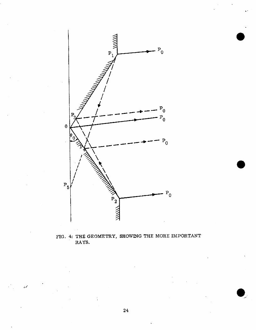
cient to describe the analysis in terms of slope discontinuities. The geometry
is now as shown in Fig. 4, where we have included the ray paths to be considered.
Observe that because of the azimuthal symmetry of the problem, all rays reaching
P are confined to a single plane through the z axis.
Let us begin by establishing some of the more important path lengths and
angles associated with the rays shown in Fig. 4. The direct--ray is OPO, and
[1OPO = r by definition. The two simple diffracted rays are OP ~PO and 0P2P0.
Since the interior half wedge angle ~ is
0’ ;(7-6.)
and ~P ~OPO = @-0., the diffraction angle
Q“.
(38)
y (see Fig. 3) for the upper path is
en(39)
23
. .
1----1
FIG. 4: THE GEOMETRY, SHOWING THE MORE IMPORTANTRAYS.
24

Also,.
● [PIPO]= .- [OP~COS~PIOPo = .-d.os(@-Oo) (40)
where d is the slant length of the cone. For the lower path OP P~ o, the cor-
responding results can be obtained by replacing 6 by ~ -0.
The two diffracted-reflected rays are OP i P4P0 and 0P2P3P0. For the
former, L 0P4PL = r -@o-6 and hence ~OPl P4 = 30.+0 -r. If this path is to
exist, it is necessary that
! o<3eo+e-w30
where we + d excluded the extremes for which the reflection point coincides with
either the ource O or the surface singularity P2, and thus‘7
T-360 <8 <T-260 (41)
showing that 00 must exceed r/4. The diffraction angle y for this path is
; 560
‘i~ 7. —+6-7 . (42)2,.
Moreover, ‘~rorn triangle 0P1P4,
“[ 1
d sin 200
[]
d sin(360 + 6-~)P1P4 = 0P4 ‘ (43)
sin(6 ++3.) ‘ sin(7r -6-60),i!.’-.
and hence ,’
[1‘4P0= r -d sin(8+ 36.) cot(tl +60) (44)
For the other path the corresponding results can again be obtained by replacing 0
by ~ -6, In particular, the criterion for existence of this path is
2f10<b <360 . (46)
25
.
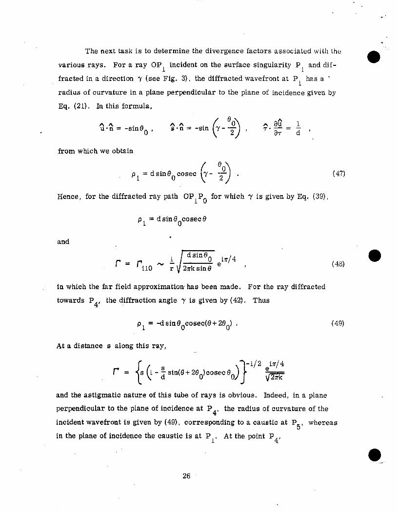
The next task is to determine the divergence factors associated with the
various rays. For a ray OPl incident on the surface singularity P ~ and dif -
fracted in a direction ‘y (see Fig. 3), the diffracted wavefront at P, has a “
radius of curvature in a plane
Eq. (21). In this formula,
64u*n= -sin$
o’
from which we obtain
perpendicular to
AAS“ri=
(
-sin Y -
J.
the pLane of incidence given by
()‘o= dsineocosec y- ~ .
~1
Hence, for the diffracted ray path OPLPO for which Y is given by Eq. (39),
= d sin60cosec6‘1
.and
in which the far field approximation has been made. For the ray diffracted
towards P4, the diffraction angle T is given by (42). Thus
‘1 = -d sin 6ocosec(6+ 28.) ,
At a distance s along this ray,
{(r=sl - ~ sin(tl + 2@o)cosec 0$-1/2 eg
and the astigmatic nature of this tube of rays is obvious. Indeed, in a plane
perpendicu~ar to the plane of incidence at P4, the radius of curvature of the
(47)
(49}
incident wavefront is given by (49), corresponding to a cauatic at P5’
whereas
in the plane of incidence the caustic is at P ~. At the point P4,
26
9
.
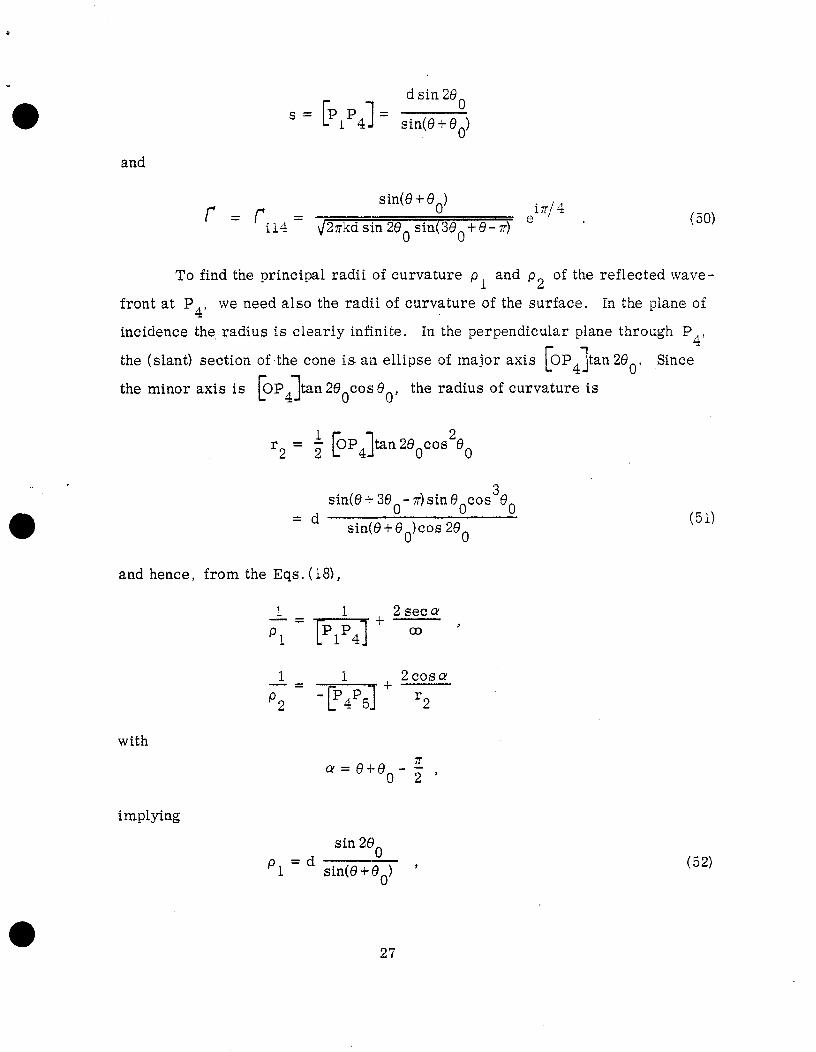
d sin 260
[1S=PP=14 sin(6+f30)
and
sin(e+$o)r = ri14s ~i7r/4
/2mkd sin 260 sin(360 +8 - r)(50)
To find the principal radii of curvature p ~ and p2 of the reflected wave-
front at P4, we need also the radii of curvature of the surface. In the plane of
incidence the, radius is clearly infinite. In the perpendicular plane through P4,
[1the (slant) section of the cone is an ellipse of major axis 0P4 tan 26.. Since
[1the minor axis is 0P4 tan 260COS 6., the radius of curvature is
[1L 0P4 tan 2@ocos260‘2=2
sin(e + 3@o
-T)sin@ocos3@d
o=sin(6+@o)cos 20
0
and hence, from the Eqs. ( 18),
:= TZ$J+-’;=+Z’I+2Y
implying
sin 28d
o‘1 = sin(6+60) ‘
(51)
(52)
27’

Qsin2$Ocos26&in(380 +6-r)
‘2=4(53)
sin(9+$O) {sin(6+60)cos Z@O- $ cos300sin(6’ + 26.)] “
The divergence factor for the reflected tube of rays is therefore
(54)
in which the far field approximation has been made,
We can now start assembling the ray contributions to the radiated fieid
at P o. For the direct ray OPO from the source we have, from Eq. ( 1),
A(w)E(PO) = ~ e
ik(r -et)(55)
where the symbol E will be used throughout to denote the 6 component of the
electric field. For the diffracted ray OPIPO,
1)ik([PIPO -etE(PO) = Ei(P1)Driloe . (56)
Since the diffraction angle ‘y is given by Eq. (39), the diffraction coefficient D
for a slope discontinuity is, from
Ds($) =
with
Eq. (36),
2k sin kn-~Osk~+cOske
(57)
h ()‘o ‘1= 1+7 , (54
whereas for a curvature discontinuity,
0.,

. 2’ ‘H.w422LDC(8)= ~ —{Cos,o.cos[+!$y
from Eq. (37). For brevity we shall denote both Ds(t?) and DC(0) by the same
symbol D(e). Also,
A(u)Ei(P1) = w e
ik(d -et)
o(60)
where the factor 2 appears because GTD requires only the incident rather than the
total field arriving at a singularity, and at grazing incidence, the former is one-
half of the latter. On inserting this expression into (56) and using (40) and (4d),
the contribution of the diffracted ray OPIPO is found to be
E(PO) x
- :R’(e)ei”’’;k’r+d-dcos(e-’o’-ct:,l) -
The contribution of the diffracted ray 0P2P0 differs only in having ~ -6 in place
of 9.
For the diffracted-reflected ray OP ~P41?0,
ik[PlP4] ik( [P4PO] - et)‘ E(I?O) = Ei(Pl)DPi14e Rrlae .
Comparison of the diffraction angles (39) and (42) shows that
Also, for a
(45) , (50,
(62)
D s D(27-200-8) .
normal component of the electric field, R = 1. Hence, from Eqs.
and (54), the contribution of this ray is .

.
A(&))coseo
/
cot eo
E(PO) - ~r~ cos3eosin(0+ 26.)]rkd{sin(e +60)cos ~eo- ~
i!<{r+d -dcos(~+ 36.) -et]
. D(27r-260-6)eiT/ 4 ~ . (63)
Since the contribution of the ray 0P2P3P0 again differs only in having 7-6 in
place of 6, the far zone radiated field at PO correct to the first two orders of
k is
ikd cos(e + 8.) -ikd COS(O+ 36.)
+D(r-$)e + v1F(@~2~ -260-6)e
where
ikd COS(W -0),0
+ ~2F(~-e)Mm-2eo+f3)e }1 (64)
/
sin6 cos3@F(6) =
o . (65)
2 sin(6 + 190)cos 26.- c0s3$osid@ + 26.)
In Eq. (64), vl = O unless
when v1
= 1, and V2 = O unless
260<0<360
when v =2
1, with the additional restriction that 60<6 ~ 7r/2. When normalized
relative to the direct radiated field of the source, the perturbation field is there-
fore
30

,J-:++ikd~(,):i’’’’’’o-’o’+D(T_,):’’cos(e+80’6E(PO) = A
-ikd COS(8+ 30.) ikdcos(3610-t?)
+ v1F(@)D(2r-200-6) e +v2F(~-t?)D(r- 2tlo+@)e
1
(66)
‘3/2) for a discontinuity in‘1’2) for a slope discontinuity, but O(kwhich is O(k
curvature.
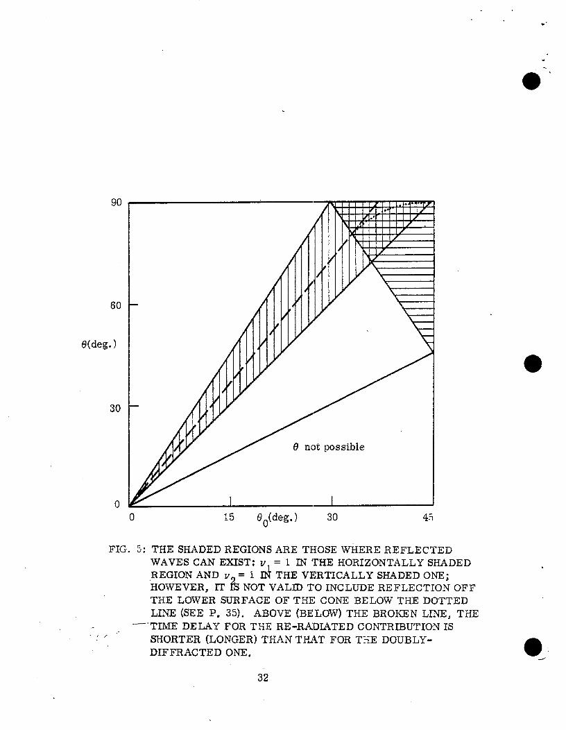
The diffracted-reflected rays can only exist for restricted ranges of 6’
and to better appreciate when either or both of the last two terms in (64) and (66)
are present, Fig. 5 shows the situations in which v ~ = 1 or V2 = 1‘ for 190< 7r/4.
Observe that neither reflected ray can occur if 380< e < IT/2 and that v ~ = o for
all ~ if 60< 7/6.
4.2 Time Domain
For a voltage pulse applied across the gap, the early time behavior of
the radiated field can be obtained by the inverse Fourier transformation of the
asymptotic expansion (64) for E( PO). The particular source voltage that we
shall consider is the unit step function U(t) for which (see Eq. 3)
A(u) = ;fo , (67)
and the contribution to the field produced by direct radiation from the gap is
{
f.E(PO) = #
~ eiur/cu r sine
}
f.=— U(t - :) .
r sin O
The diffracted and diffracted-reflected contributions then appear at times which
are delayed by amounts proportional to the increase in path ‘length.
To simplify the subsequent presentation of the data, it is convenient to
● take the origin of time at the instant at which the direct contribution arrives at
31
.
90
60
6(deg. )
30
00 15 f30(deg.) 30 45
FIG. 5: THE S13ADED REGIONS ARE THOSE WfiERE REFLECTEDWAVES CAN EXIST: v = 1 IN THE HORIZONTALLY SHADEDREGION AND V = 1 Id THE VERTICALLY SHADED ONE;HOWEVER, IT ?3 NOT VALID TO INCLUDE REFLECTION OFFTHE LOWER SURFACE OF THE CONE BELOW THE DOTTEDmm (SEE P. 35). ABOVE (BE Low) THE BROmN mm, THE
‘—-TIME DELAY FOR THE RE-RA.DIATED CONTRIBUTION 1S,.SHoRTER (LoNGER) THAN T.Hi4T FOR TXE DOUBLY-DIFFRACTED ONE, 0!’
32

. the field point PO, and to measure time in nanoseconds. Since the velocity of
light is, in MKS units, 3x10” m/see = O. 3 m/nsec approximately, it follows
that in all formulae from now on,
measured in meters (of course).
diffraction contributions are now
c must be given the value O. 3 with distances
The time delays associated with the various
t(=:{ 11 -Cos(e-eo) , t2 = : {l+cos(e+eo)} ,
(6d)
d {I -cOs(e+ 36.)] , t4 = ~ {1+ COS(6 - 30.)] .‘3=:
Observe that if tl = tl(e), we have
‘2= tp) ,
‘3= tl(27r-3eo-e) ,
‘4= p 3eo+6) .
It is also convenient to normalize the fields by suppressing the factor fO/r sin f3.
Using now the inverse Fourier transform (9), the time domain expression
for the normalized electric field at the point POwhen Pl and P2 are slope dis -
continuities is
E=J= [
u(t) + ~ Ds(6)(t -t$/2U(t -tl)+Ds{@)(t -t2)1/2U(t -t2)
+~1F(e)~s(2~-2$o-e)(t-t3)1/2u(t+3)
1+~2F(T-(@(~-260+@(t -t4)1/2u(t -t4) (69)
where DS(6) is given in Eq. (57). Similarly, for a discontinuity in curvature,
‘ +/”[E = U(t)+ m)(t -tp%(t -tl)+m-e)(t -t2)WJ(t -t2)
+ V1F(6)6C(27P 260-@(t -t3)3’2u(t -t3)
1+p2F(T-6)6c(p260+6)(t -t4)3’2iJ(t ‘t4) (70)
33

.
where.
●
and hence, from Eq. (59),
4.al Moseocc++ :)tic(e)= - -y--
foseo-cos(+) )}’ “(71)
As we have previously remarked, the criteria for validity of an approximate
solution in the frequency and time domains are somewhat different, and just be-
cause all four diffracted and diffracted-reflected contributions are of the same
order in k does not imply that it is legitimate to include them in the time domain
solution. An upper bound on the time duration for which our solution couid be
valid is provided by the shortest ray path whose contribution is omitted, and
since we have not included any double diffraction or re -radiation contribution, a
necessary condition for validity is
t<T
where
T=d: min.
{ )2, l+2cos130- cos(e-eo) . (73)
The angle 6 for which
2 = l+2cos60-cos(&f30) (74)
is plotted as a function of 19~, 80<45°, as a broken line in Fig. 5, Above this
line
2< l+2coseo-cos(&60)
so that the omission of any re-radiated contribution is now the more restrictive,
whereas below the line
2> ~+2c0. eo-c0.(e-eo) ,
34

*
.
making doubie diffraction the basis for our criterion. For t10 >36.9°, Eq, (74)
has no solution for 6 ~ 90°.
For the contribution produced by diffraction at the lower surface singularity
P2 and then reflection off the upper surface of the cone, the associated time delay
is t~, and it can be verified that
for all 6 for which the path exists. At the lower boundary of the vertically shaded
region in Fig. 5,
g
‘4=C { }l+2coseo-cos(e-eJ < :
and at the upper boundary
‘4 =f<:
{1+2 cosf30-cos(6-80)] ,
and since t4 < T throughout the interior of the region, it is legitimate to include
this contribution in our time domain solution.
The situation is rather different for the contribution which results from
reflection off the lower surface of the cone. It is obvious that t3 ~ t4 with
equality only for 19= 901 and t3 ~ 2d/c. with equaiity on the lower boundary
of the horizontally shaded region in Fig. 5, Throughout most of this region, how-
ever, T is determined by the doubly diffracted ray, and t3 < T only at those
points of the region lying above the dotted line in Fig. 5. For most practical
purposes, therefore, this reflected ray contribution is of no interest in the time
domain.
35

.,
,,
.5. Data and Coriclusions.
Expressions for the normalized transverse electric field E at a point
(rj G) in the far zone of the biconical portion of theantenna aregiven as functions
of the eiapsed time t in Eqs. (69) and (70). The first of these applies to the case
of a cylindrical continuation which produces a slope discontinuity at the junction,
and the second to a hyperbolic continuation for which the discontinuity is
vature. Both are vaiid for only
sufficient) condition for validity
required that
a short range of times, and a necessary
is that given in Eq. (72). In particular,
t<”= ad
in cur-
(but not
it is
(75)
where t is measured in nanoseconds and d in meters.
Each of the expressions for E(t) is valid for 00 f 6< 7r/2 and consists
of a direct contribution from the source and up to four secondary contributions
produced by diffraction and diffraction-reflection. AH of the contributions are
entirely real and since Ds(tl) and ~c(6) are negative for 60<6 ~ r/2, thee
secondary contributions subtract from the direct one. These properties are
physically required. With increasing t, each secondary contribution increases1/2
as (t -ti) or (t-t )3/2 according as the discontinuity is in siope or curvaturei
respectively, where t = ti is the time of onset. Of necessity, there must now:::
exist a time t = ti at which the secondary contributions are the same for the two
geometries, all other parameters being equal. For O<t<t~, a discontinuityL .,,
in curvature produces the smaller perturbation, whereas for t > ti a slope dis-,.
continuity is preferable. Each secondary contribution has its own associated,,:
‘lcrossing time” ti and there is obviously an analogous time t’~ appropriate to
the sum of all of them..,.-,-
A knowledge of t in relation to the upper limit T of validity of our
treatment is one of the key factors in assessing the relative merits of the two*-
geometries. Unfortunately, t can in general be obtained only from an exarnina -
tion of computed data, but in the particular case where 6 = T/’2 and the reflected
contributions can be ignored, e .-
36

>k nsi=lmL
Hence, from Eqs. (57), (71)
showing an
can ensure
.,.t 4’-,1 J-g
-15C( T/ 2)
and (14),
2X sin AT
COSA,+C?C)S+
(c.st?,-sin $)3
( )
‘osin 26 0 l+cosoo sin ~
(76)
(77)
increase proportional to e and d. By choosing e large enough, we
that the curvature discontinuity produces the smaller perturbation
throughout the entire range of’ times t < T for which our analysis is valid, and the
value of e for which t’x = T has been computed from Eq. (77) and is plotted as a
function of 00 in Fig. 6.
For values of 6 other than 7r/2 it is necessary to turn to computed values
of E(t) to draw any conclusions about the performance. A computer program has
been written to calculate E(t) from Eqs. (69) and (70) for any combination of para-
meters. The program is quite straightforward and needs no comment, and in
analyzing the data, the only complication is that produced by the number of
parameters involved. The variation of the field strength with time is a fum tion
of 0, 60 and d and, in the case of a curvature discontinuity, of ~ as well. For-
tunately, however, the effect of some of these parameters is rather trivial. Thus,
~ affects the perturbation produced by a curvature discontinuity only as a scaling ,
factor: an increase in e by a factor 2 decreases the perturbation by the same
amount. The slant length d affects proportionally the times
secondary contributions reach the field point (see Eqs. (68))
changes the magnitudes of all perturbations through a factor
dependence of E(t) on 6 and 60 is much more involved.
ti at which the
and, in addition,
d-1/2, but the
The form of the computer output is illustrated in Tables i and 2 which
show the normalized early time response, E(t), as a function of t for’f @@90 ,0
“e= O implies a slope discontinuity and, hence, Eq. (69), whereas c # Ocorresponds to a cul*vature discontinuity, i. e. Eq. (70).
37

..-.
145
1.0
e
0.5
0
.
.
10 20 30 40 50$O(deg.)
FIG. 6: THE FRACTIONAL INCREASE, e, IN RADIUS FOR WHICH.!.t~ = T WHEN 19= 90°.
. .
,,
38
●✌
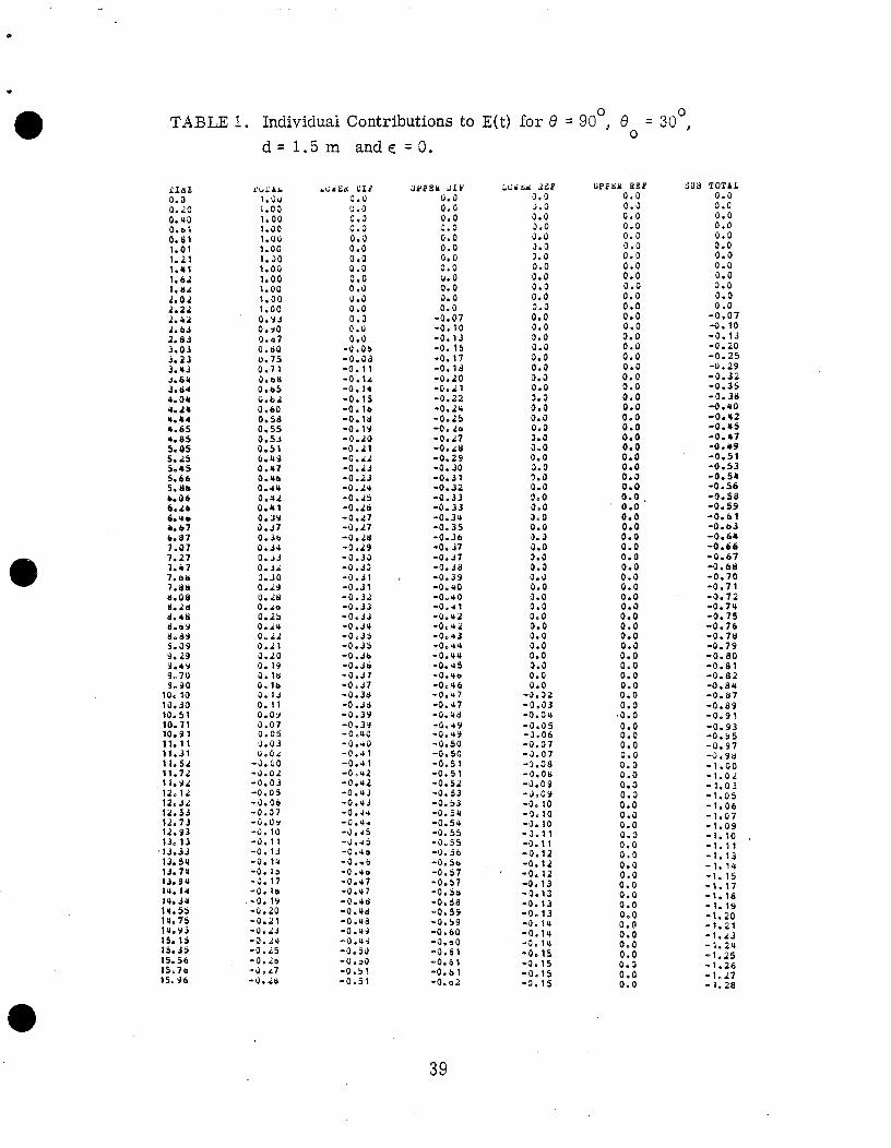
TABLE 1. Individual Contributions to
fSd E0.00.200.43O.bl0.811.011.211.411.621.8A2.022.222.422. bJ2.833.033.233.434.643.844.044.24*.k44.654.855.955.255.45%665. U*b. Li13
6.266.u6b.67h877.077.277.471. b~
1.88*.08&2dd.4tli3.698.$9S.099. .?99.499.709.90
10.1010.3010.5110.7110.9111.1111.3111. 5,211.7211.9412.1212.3212.5312.7312.93t3. 13
13.3313.5413.7413.9414.1494. J414.5s14.7514.9515.15:5.3s15.56ls.7b15. 9b
d=
iu’L4kl.dd1.001.001.001.001.001.001.001.001.001.001.000.930.900.67O.do0.7s0.710.b80.b5O.bd0.600.5130.550.5s0.516.490.470.4b0.4U0.4,?0.410.390.J70.3b0.340.J30.J29.300..290..280.200.25oei40..220.210.200.19a. 180.160.130.110.030.070.05LI.03U.04
-J. (JO-0.02-0.03-0.05-d.06-0.07-0.05-d. 10-0.11-0. lJ-o. 14-0.15-0.17-0. lu-0.19-0.20-0.21-O*JJ-0..44-0.25-0.20-Q*L7-o.2a
l,5m andc’O.
0.00.00.00.40.00,00.00.0O.uU.o0.00.0O.u0.0
-0. Ob-0. oa-0.11-0. lA-0.1*-0.15‘0. lb-0.18-0.19-0.20-0.21-0..42-0.23-0.23-0..lti-0.25-0..26-0..)7-0.27-0.28-0.29-0.3.3-0..I2-0.31 ,-0.31-0..),?-0.33-O*3J-0. J4-0.35-0. JJ-0. Jb-0.36-9,37-0. J7-0.38-0.3d-0.39-0.39-C.40-0.40-0.41-0.41-0.+2-0.$2-0.43‘o. QJ-0.44‘0. Q14-d. *5-d.45-0.43-0.46‘(?.40-0.47-O. *7-o.4d‘Oe4d-0.48-0.+9-o. @’J-U.50-0.50-0.53-0.51
0.00.00.00.00.00.00,00.0(J. O0.00.00.0
-0.07-0.10-o, 13-0.15-0.17-0.18-0.20-0. J.1-0.22-0.24-0.25-o. Je-0.47-o. &u-0.29-0. 30-0.31-0.32-0.33-0.33-0.34-0.35-0. Jb-0, 37-0.37-0.38-0.39-0.40-0.40-0.41-0.42-0.42-0,43-0.44-0.44-0.45-0.40-0.46-0.+7-o. U7-0.48-0.49-0.49-0.50-0.50-0.51-0.51-0.5.2-0.53-0.53-0.54-0.54-0,55-0.55‘0.5b-o.5b-0.57-0.57-0.58-0.58-0.59-0.59‘0,60‘0. bo-0.61-0.61-0. bl-0.02
E(t) for e = 90°, e. = 30°,
Lud Ld .42P0.0d.o0.09.00.0J.O).00.00.03.00.02.0O*O0.00.0U.o0.00.00.00.02.00.00.0U*O3.03.00.03.0‘).00.05s00.0Jao0.00.00.02.00.0O.d0.00.00.00.00.00.09.00.00.00.00.0
-3.92-0.03-0.04-Oaos-J.06-0.07-J .07-9.0$3-0.08-!3.09-J .09-0.10-9.10-o. 10-3.11-0.11-0.12-0.12-0. 12-0.13-0.13-0.13-Oa 13-0.14-0.14-O*14-0. 15-0.15-0+15-0.15
UPPiH REP0.00.00.00.00.00.00.0
MM0.00.00.00.00.00.00.00.00.00.00.00.00.00.00.00.00.00.00.00.0,0.00.00.00.00.00.00.00.00.00.00.00.00.00.00.00.00.00.00.00.00.0
.0.0
0.00.00.00.00.00.00.00.00.00.00.00.00.00.00.00.00.00.00.00.00.00.00.00.00.00.00.0
SUB TOTAL0.00.00.00.00.00.00.00.0!).00.00.00.0
-0.07-0.10-0.13-0.20-0.25-0.29-0.32-0.35-0.38-0.40-0. s2-0.45-0.47-0.49-0.51-0.53-0.56-0.56-0..58-0.59-0.61-o.133-0.64-0.66-0.67-0.68-0.70-0.71-0.72-0.74-0.75-0.76-0.78-0.79-0.80-0.81-0.82-0.84-0.87-0.89-0.91
-0.93-0.95-0.97-0.98-1.00-1.0/!-1.03-1.05-1.06-1.07-1.09-1.10-1.11-1.13-1.14-1.15-1.17-1.18-1.19-1.20-1.21-1.43-1.24-1.25-1.26-1..f7-1.28
39

TABLE 2: Individual Contributions to E(t) for6 =90°, ,60 ‘30°,
7.077.271.477.6*7.UUa.oti8.2#8.488.6’9*. ki99.9$+9.299.499.7a9.9a
to. laIO*JO10.51tollk?. 91
12.3J12.5312.7312.*3
d=l.5rn and
LuIAL1.001.00l.o~1..230.99a.970.940.91IJ.870.630.7*[email protected]#0.110. 1+6.07
-0.0 1-0. cal-a. w-0.24-0.3A-0.41
.-0.50-a.59-0.68-43.77-13. d7-a. sb-1.l)b-%. 10-1.,it-t. J7-i.4J-1.%1-1.69-1. MO-1.91-i. a3-2. 1*-2. 2*-4. W-.t.50-L.6L-J. 74-,z. d6-i.9j-3.11-3.24-i. il-J .50-3.6J-3.77-3.90-*.04-4.11-+.31-4.45.-4.5’4-.).71-4. dd-3.04-5. 17-j. Jl->.4*-5.01-5.70-> .91-U. co-G. AI-G.37-~.5.2‘o. b@
-0. tl.l
Ludi!i LtLtd.oO.JC.a0.!30.00.00.0a.o0.0o.aa.~0.00.00.0O.J0.00.00.30.00.00.00.0O.J0.00.0o.a0.9
-0.00-0.do-a.s~-0.0 t-0.01-a.o~-a. a~-0.0.?-0.od-b.03-0.04-0.04-0.05-0.05‘0. Ob-0.07-0. J7-0. od-o. a9-0.09-6.10-0.11-0.12-0. 1,+-O.l J-0. tu-0.15-0. lb-0.1?-0.17-0.16-0.19-o. &fJ-0../ I-Q.22-0..2J-0.24-a..25‘C. db
-0..?7-0..?5-0.29-o .40-3.31-0.4.4-0. JJ-0.34-0. db-0. J7-Old-0. JY-0.40-0.41
= 1,
ukti~d LU.?a.a0.00.0
-0.00-a. ol-0.03-0.06-o. a~-0.13-0.17-0.21-0..26-0.31-o. Jb-0.41-a.47-0. >3-0.59-0. b6-0.72-0.79-0.46-o. !33-1:01-t. oti-1.16-1.24-1.32-1. ut-1.49-1.51J-1.67-1.76-I .*5-1.94-2.03-2. 13-2.23-2.33-2.43-A. 53-2.63-.2.73-2.44-2.95-3.05-3.16-3. .?7-3.39-3.50‘3. bl-3.73-3.$5-3. Y7-4. a9-4.21-4*A3-4.45-6.57-4. 70-4.83-u’. !)5-5. Oa-5.2!-5.44-5,47-5.61-5. /u-5*67-b. al-e. li-b, JY-0.42-6. >b-b. 71-6. M5-b. YY
-7.13-7. dli-7. UJ
LUSU 4JFJ.o1.03.0J.o.?.0d.a
;::J.o0.9
NJ.a0.0J.a‘3.09.a0.0il. o3.00.00.00.04.00.0a. oJ.110.00.0o.a0.0o.a0.00.00.0
M0.00.0
M
M0.00.09.00.30.00.00.00.0
N’
::!0.0~.aJ.J3.09,0O.dJ.o0.00.0J.a1.03.03.0O.u3.03.00,0J.Ll].a0.0.3.0J.clJ*Od.o0.0
UI?PZU Ml!0.00.00.0o.a0.00.00.90.0o.a0.00.00.00.00.0a.o0.0o.a0.00.00.00.0a.o0.00.00.0o.aa.o0.0o.a0.00.00.00.00.00.00.0o.a0.00.00.60.00.00.00.00.0o.a0.00.00.00.0(7.00.00.00.00.0a.o0.00.00.00.00.0o.a0.0
:::o.a0.0
::;0.0G.o0.00.00.00.0G.oG.oo.a0.0a.o
SUB TuTALa.o0.00.0
-9.00-oat-0.03-0.06-0.09-0.13-0.17-0.21-a.26-0.31-0.36-0.41-0.47-0.53-0.59-0.46-0.72-0.79-0. i56-0.93-).01-i. os-1.16-1.2U
-1.32-1.41-1.50-*.59-1.68-1.77-1.87-1.96-2.06-2. 16-2.26-.4.37-2.67-2.5E-2.69-2* aa-2.9 1-3.03-3.14-3.26-3.38-3.50-3. b2-3. ’lb-3.86-J. 99-4.11-4.24-4.37-$.50-4.63-4.77-4.90-5. a4-5. 17-5.31-5.&5-5.59-5.73-5.8a-b.02-0. 1?-6.31-6.46-b.6 1-6.76-6.91-7.06-7.21-7.37-7.52-7. ba-7. h4
40

●
.
0“
~ = O and f3~60°, e = 1, the cdkr parameters b;ing the same (d = 1.5 m,
‘o~ 300). The total field is broken down into its various components and the
last column (labelled “sub-total”) is just the sum of the four previous columns,
i. e. the net perturbation. Although T ~ 10 nsec for both Tables, we have in-
cluded data for times up to 16 nanoseconds to demonstrate the increasingly neg-
ative value of the field amplitude as t increases. Indeed, as t -+ co, E(t)+ -co,
but this is just a consequence of the failure of the initial time approximation.
As noted earlier and evident in Table 1, the reflected field for 0 = 90° comes
in just before the limit of allowable times and only achieves a significant mag-
nitude at times which are greater than those that can be entertained. For values
of e markedly le~s than 90°, the same conclusion holds for the diffracted con-
tribution of the lower discontinuity (see Table 2). Thus, for most practical pur -
poses, it is sufficient to ignore any contribution due to reflection, i. e. put
‘1=V2= O in Eqs. (69) and (70) for all 6 and @o, and, in addition, include only
one diffracted contribution when e differs markedly from 90°.
The effect of changing from the slope to a curvature discontinuity is
illustrated in Fig. 7 for the case in which d = 1.5 m, 00 = 29°, @= 90° and
e = 1. The crossing time t* is 8.3 nsec, which is not far short of the limit
T = 10 nsec for which the solutions are admissible. As judged by the magnitude
of the field perturbation, this particular curvature discontinuity is superior to
the slope discontinuity over most of the admissible time span, and to increase
e or d enhances this superiority. When 6 = 90°, the contributions from the
upper and lower bicones and discontinuities come in at the same time, bat this
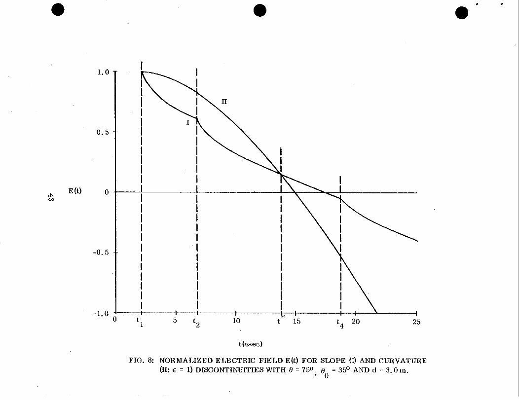
is not true for 0 # 90°. This is illustrated in Figs. 8 snd 9. In both cases
d = 3.0 m and the curves are for a slope discontinuity (e ‘ O) and a curvature
discontinuity having e = 1. In Fig. 8, @= 75° and 00 = 35° for which the
maximum allowable time is T = 18.7 nsec. The breakpoints associated with
the two diffracted contributions are clearly differentiated and even the contribution
due to reflection off the lower bicone enters within the allowable time span, as.
predicted by Fi&. 5. The curve for the curvature discontinuity has these same
●breakpoints, though they are not so immediately apparent.
41

0,5
E(t)
o
u 3 4 6 8 r’” 10t (nsec)
FIG. 7: NORMALIZED ELECTRIC FIELD E(t) FOR SLOPE (1) ANDCURVATURE (II: e = 1) DISCONTINUITIES WITH 6 = 90°, 00 = 29°ANDd=l.5m.
. . .,,f
,“””
42
I&GJ
E (t)
1.0
0.5
0
-0.5
-1.0
i I
I I II
iI I
IIIIIIIIII
-1
Ot1
\
I
\
iI III II II II 1“1 I
1 t 1 I 1 ,u
a \
5:
‘210 t 15
‘420
t (nsec)
-i
25
FIG. 8: NORMALIZED ELECTRIC FIELD E(t) FOR SLOPE (I) AND CURVATURE
(II: 6 = 1) DISCONTIN(JITIES WITH 0 = 750, e. = 35° AND d = 3. Om.

1.0
0,5
I@I& E (t) o
-O* 5
-1.0
IIII
I
I III II II I
I I I
I ! I# 1
‘1 5 t* 10 t2
t(nsec)
FIG. 9: NORMALIZED ELECTRIC FIELD E(t) FOR SLOPE (I) AND CURVATURE(II: e = 1) DISCON INUITIES WITH 6 = 57°, (30 = 29° AND d = 3. Orn.
b ● /b
,
*
..
.
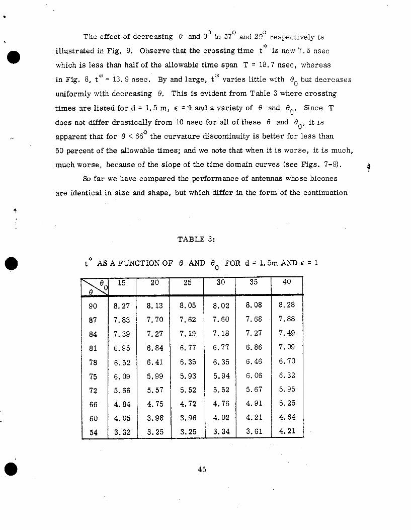
The effect of decreasing 19 and O“ h 57° and 29° respectively is
illustrated in Fig, 9. Observe that the crossing time t ‘;: is now 7.5 nsec
which is less than half of the allowable time span T ‘ 18.7 nsec, whereas>~
in Fig. 8, t = 13.9 nsec. By and large, t’;f varies little with 190but decreases
uniformly with decreasing t3. This is evident from Table 3 where crossing
times are listed for d = L 5 m, c =‘1 and a variety of 6 and 6.. Since T
does not differ drastically from 10 nsec for all of these @ and 8., it is
apparent that for 6<66° the curvature discontinuity is better for less than
50 percent of the allowable times; and we note that when it is worse, it is much,
much worse, because of the slope of the time domain curves (see Figs. 7-9).4
So far we have compared the performance of antennas whose bicones
are identical in size and shape, but which differ in the form of the continuation
TABLE 3:
;::t AS A FUNCTION OF 6 AND e. FOR d = 1. 5m AND ~ = 1
\6(
i3
90
87
84
81
78
75
72
66
60
54
15
8.27
7.83
7.39
6.95
6.52
6.09
5.66
4.84
4.05
3.32
20
8.13
7.70
7.27
6.84
6.41
5.99
5.57
4.75
3.98
3.25
~
25
8.05
7.62
7.19
6.77
6.35
5.93
5.52
4.72
3.96
3.25
30
8.02
7.60
7.18
6.77
6.35
5.94
5.52
4.76
4.02
3.34
T
8.08
7.68
7.27
6.86
6.46
6.06
5.67
4.91
4.21
3.61
40
b
8,28
7.88
7.49
7.09
6.70
6.32
5.95
5.25
4.64
4.21 “
45
c
*
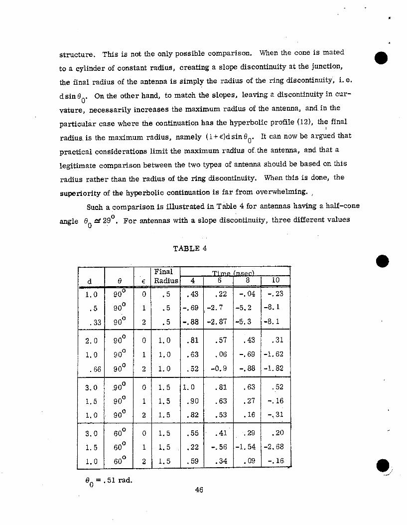
structure. This is not the only possible comparison. When the cone is mated
to a cylinder of constant radius,●
creating a slow discontinuity at the junction,
the final radius of the antenna is simply the radius of the ring discontinuity, i.e.
d sin 6.. On the other hand, to match the slopes, leaving a discontinuity in cur-
vature, necessarily increases the maximum radius of the antenna, and in the
particular case where the continuation has the hyperbolic profile (12), the final!
radius. is the maximum radius, namely ( i + e}d sin (lO. It can now be argued that
practical considerations limit the maximum radius of. the antenna, and that a
legitimate comparison between the two types of antenna should be based on this
radius rather than the radius of the ring discontinuity. When this is done, the
superiority of the hyperbolic continuation is far from overwhelming. ,
Such a comparison is illustrated in Table 4 for antennas having a half-cone
angle 190= 29°. For antennas with a S1OPSdiscontinuity, three different v~ues
TABLE 4
d 6
1.0 90°
.5 90°
.33 90°
2.0 90°
1.0 90°
.66 90°
3.0 .90°
1.5 90°
1.0 90°
3.0 60°
1.5 60°
1.0 60°
Final )E Radius 4 6 10
— —o .5 .22 -.04 -.23
1 I .5 -.69 ,-2.7 -5.2 -8.1
0 1.0 I .81 .57 I .43I
.31
1 11.0 I .63 .06 I -,69-1.62
2 I 1.0 I .52 [ -0.9 I -.881-1.82
0 1.5 1.0 .81 .63 .52
1 1.5 .90 .63 .27 -.16
2 1.5 .82 .53 .16 -..31
0 1.5 .55 .41 .29 .20
1 1.5 ● 22 -.56 -1.54 -2.68
2 1.5 .59 .34 .09 -.16
.
60= .51 rad.
46

of d are considered and the response noted at t ‘ 4, S, 8 and 10 nsec, E aoh
antenna is compared with two having curvature discontinuities at slant distances
d/ (l+e) which are such as to yield the same overall antenna radius.. The more
the response differs from 1.0, the greater the field perturbation and (for our
purposes) the poorer the antenna. As judged by the responses at the times listed
in Table 4, each of the curvature-discontinuity antennas is substantially infe rior
to the equivalent slope-discontinuity one.
This conclusion, however, is not entirely fair on several counts. To
change d changes the time T beyond which the analysis is invalid, and thus,
when d= 1.0 and e=l, T = 6.66 nsec, but when d= 0.5 and 0.33, T =3.33 and
2.22 nsec respectively. Hence, as regards the first three lines in Table 4, the
comparison with the curvature-discontinuity antennas has been made at times
far beyond the limits of applicability for these antennas. The same criticism
applies to most of the other comparisons in the Table. On the other hand, had
we concentrated on the responses at sampled times such as 1, 2, 3 nsec to
ensure the validity of the comparison, it would have been found that in almost
all cases, the slope-discontinuity antenna had a response of 1.0, showing no
~rturbation at ail, since the first diffracted contribution would not yet have
arrived. Once again, the curvature-discontinuity antennas would have been
judged inferior, aIbeit by not so large an amount.
A more fundamental criticism of the comparison is possible. We have
already remarked that the hyperbolic continuation is only one of many serving
to match the slope of the bicone. Others can be found which achieve the same
purpose but yield different values for the maximum radius of the antenna. In
practice, it is not even necessary that the continuation profile be a single analytic
curve, and having followed (say) a hyperbolic profile for some distance beyond
the upper limit of the cone, a different profile function can be introduced. Pro-
vided the new singularity which is created lies well within the shadow region, it
could even take the form of a discontinuity in slope without substantially affecting
the early time behavior. All such geometries require a much smaller (fractional)
increase in the radius of the antenna than is implied by (14) for the same discon-
47
.. .
A
tinuity in curvature, although some increase beyond that of the slope-discontinuity ?
antenna is inevitable, a
By its very nature, a discontinuity in curvature produces a smaller amount
of high frequency diffraction than a discontinuity y in S1Ope and hence, all other
factors being equal, the former is preferable as regards the early time behavior
of the antenna. The analysis we have given enables the effects to be determined,
but whether the improvement is sufficient to compensate for the increased radius
and difficulty of construction of the antenna, is a topic beyond the perview of this
report.
48*’/’

.. .’
.
J
9 References
* Fock, V. A. ( 1965), ElectromagneticPergamon Press, New York.
Hong, S. and V.H. Weston (1966), A
diffraction and propagation problems,
modified Fock function for the distribution
of currents in the penumbra region with discontinuity in curvature, RadioSci. ~, 1045-1053.
Kay, I. and J. B, Keller (1954), Asymptotic evaluation of the field at a caustic,J. Appl. Phys. &, 876-883.
Keller, J. B, (1957),
Keller, J. B. (1962),116-130.
Diffraction by an aperture, J. Appl. Phys. 2&, 426-444.
Geometrical theory of diffraction, J. Opt. Soc. Amer. ~,
Sancer, M. I. and A. D. Varvatsis ( 1971), Geometrical diffraction solution for thehigh frequency - early time behavior of the field radiated by an infinitecylindrical antenna with a biconical feed, Sensor and Simulation NotesNo. 129.
Senior, T, B.A. ( 1971), The diffraction matrix for a discontinuity in curvature,Sensor and Simulation Notes No. 132.
Senior, T. B. A. ( 1972), Divergence factors, University of Michigan RadiationLaboratory Memorandum No. O10748 -5 O4-M.
Senior, T. B. A. and P. L. E. Uslenghi ( 1971), High-frequency backscattering froma finite cone, Radio *i. 6_, 393-406.
Weston, V. H. ( 1965), Extension of Fock theory for currents in the penumbraregion, Radio Sci. 69D, 1257-1270.
.
49