The Electoral Advantage to Incumbency and Voters' Valuation of Politicians' Experience:

A Regression Discontinuity Analysis of Close Elections*

David S. Lee

UC Berkeley and NBER

April 2001

Abstract Using data on elections to the United States House of Representatives (1946-1998), this paper exploits a quasi-experiment generated by the electoral system in order to determine if political incumbency provides an electoral advantage – an implicit first-order prediction of most principal-agent theories of politician and voter behavior. Candidates who just barely won an election (barely became the incumbent) are likely to be ex ante comparable in all other ways to candidates who barely lost, and so their differential electoral outcomes in the next election should represent a true incumbency advantage. The regression discontinuity analysis provides striking evidence that incumbency has a significant causal effect of raising the probability of subsequent electoral success –by about 0.40 to 0.45. Simulations – using estimates from a structural model of individual voting behavior – imply that about two-thirds of the apparent electoral success of incumbents can be attributed to voters’ valuation of politicians’ experience. The quasi-experimental analysis also suggest that heuristic “fixed effects” and “instrumental variable” modeling approaches would have led to misleading inferences in this context.

* Matthew Butler provided outstanding research assistance. I thank John DiNardo for numerous invaluable discussions, and Josh Angrist, Jeff Kling, Jack Porter, Larry Katz, Ted Miguel, and Ed Glaeser for detailed comments on an earlier draft. I also thank seminar participants at Harvard, Brown, UIUC, and Berkeley for their additional useful suggestions.

1 Introduction

An essential element to the principal-agent approach to understanding politician and voter

behavior is the notion that political incumbents act in ways to raise their chances of re-election

and to further their political careers.1 A number of economic analyses have focused on the various

mechanisms through which this might occur. For example, incumbents may influence tax and ex-

penditure policy or monetary policy, use the office to sell political favors in exchange for campaign

contributions, or vote on legislation in a way that reflects the ideological make-up or economic in-

terests of their constituencies; these things are done in order to influence voters to support their

re-election bids.2 There is an implicit empirical prediction of many of these hypotheses. Winning

an election, by definition, allows a politician to be the incumbent. In turn, only an incumbent

is able to the choose actions of an elected official; any non-incumbent candidate, by definition,

cannot choose these actions. In equilibrium, if the incumbent’s actions are meant in part to gain

electoral support, then winning an election (and hence becoming the incumbent) should have a

reduced-form positive causal effect on the probability of being elected in a subsequent election.

To what extent does that causal relationship hold empirically? The political science lit-

erature has been careful to recognize that answering this question, and measuring the electoral

advantage to incumbency, is not as straightforward as the casual observer might think.3 Through-

1 This paper incorporates and extends the material in an earlier, prelimnary draft under a different title [Lee, 2000].2 Studies that adopt a principal-agent framework in examining the political economy of elections and politicianbehavior is too voluminous to review here. The following are only a few examples of studies that consider suchhypotheses. Rogoff [1990], Rogoff and Sibert [1988], and Alesina and Rosenthal [1989] consider how incumbentsmay manipulate fiscal or monetary policy to gain electoral support. Besley and Case [1995a,b] consider the tax andexpenditure-setting behavior of incumbents, and Levitt and Poterba [1994] consider how Congressional Representa-tion might effect state economic growth and the geographic distribution of federal funds. Levitt [1996] considers therelationship between constietuent (and own) interests and ideology and politician voting behavior in Congress. Thisis also the focus of the studies of Peltzman [1984, 1985], and Kalt and Zupan [1984]. That politicians are behavingin a way (potentially by catering to special interests groups) to raise campaign funds, to raise re-election chances isimplicitly or explicitly examined in Levitt [1994], Grossman and Helpman [1996], Baron [1989], and Snyder [1990].3 The empirical literature in political science that addresses the measurement of the incumbency advantage is large.A partial sample of studies that consider the potential selection bias problems include Erikson[1971], Collie [1981],Garand and Gross [1984], Jacobson [1987], Payne [1980], Alford and Hibbing [1981], and Gelman and King [1990].

1

out the latter-half of the 20th century, Representatives in the U.S. House who sought re-election

were successful about 90 percent of the time.4 However, incumbents may enjoy re-election success

for reasons quite apart from their incumbency status. After all, there are many potential reasons

why politicians are able to become incumbents in the first place. As an example, they could be in

Congressional districts that historically favor the incumbents’ political party. In principle, this one

phenomenon – persistent heterogeneity in partisan make-up of voters across Congressional dis-

tricts – could, by itself, generate the observed 90 percent incumbent re-election rate.5 In general,

no structural advantage to incumbency is needed to explain this empirical fact.

Using data from elections to the United States House of Representatives (1946-1998), this

paper produces quasi-experimental estimates of the true electoral advantage to political incum-

bency by comparing the subsequent electoral outcomes of candidates (and their parties) that just

barely won elections to those of candidates (and their parties) that just barely lost elections. Under

mild continuity assumptions, these two groups of candidates are, as one compares closer and closer

electoral races, ex ante comparable in all other ways except in their eventual incumbency status.

The design thus approximates the ideal classical randomized experiment that would be needed to

test the incumbency advantage hypothesis, as well as the implicit prediction of political agency

theories. The identification strategy in this context is recognized as an appropriate example of the

regression discontinuity design, as described by Thistlethwaite and Campbell [1960] and Camp-

bell [1969], more recently implemented in Angrist and Lavy [1998] and van der Klaauw [1996],

and formally examined as an identification strategy in Hahn, Todd, and van der Klaauw [2001].

In the analysis, I derive a simple structural model of the individual voter’s valuation of political

experience that permits an interpretation of the magnitude of the estimated effects.

The empirical analysis yields the following findings. First, incumbency has a significant

4 Jacobson [1997, p. 22].5 I sometimes refer to this alternative story as a “spurious” incumbency effect.

2

causal effect on the probability that a candidate (and her political party, in general) will be suc-

cessful in a re-election bid; it increases the probability on the order of 0.40 to 0.45. The magnitude

of the effect on the two-party vote share is about 0.08. These findings are consistent with the

“reduced-form” prediction of the prototypical political agency model. Second, after accounting

for the selection bias, losing an election reduces the probability of running for office in the sub-

sequent period, by about 0.43, consistent with an enormous deterrence effect. Third, under the

maintained assumptions of the structural model of individual voting behavior, the estimates imply

that voters place a fairly modest value on political experience when evaluating political candidates.

One additional term of political experience (relative to the opposing candidate) would lead to a 2 or

3 percent increase in the vote share. On the other hand, small magnitudes in terms of the vote share

can have enormous impacts on the eventual election outcomes. A simulation using the structural

estimates imply that most (two-thirds) of the apparent electoral success rate of incumbent parties

could be explained by a political experience advantage that incumbents typically hold over their

challengers. Finally, I show evidence that in this context, both a “instrumental variable” and “fixed

effect” analysis of the same data lead to misleading inferences.

The paper is organized as follows. Section 2 reviews the stylized facts of incumbency

and re-election in the U.S. House of Representatives in the latter half of the 20th century. It also

provides an illustration of how the regression discontinuity design accounts for selection bias in

testing the structural incumbency hypothesis. Section 3 establishes the continuity assumptions that

are crucial to the research design. Section 4 reports the main reduced-form estimates of the causal

effects of incumbency. Section 5 develops a structural framework for interpreting the magnitude

of the effects in terms of the individual voter’s valuation of political experience. In section 6,

I compare the main estimates to that obtained from alternative “differencing” and “instrumental

variable” approaches to identification. Section 7 concludes.

3

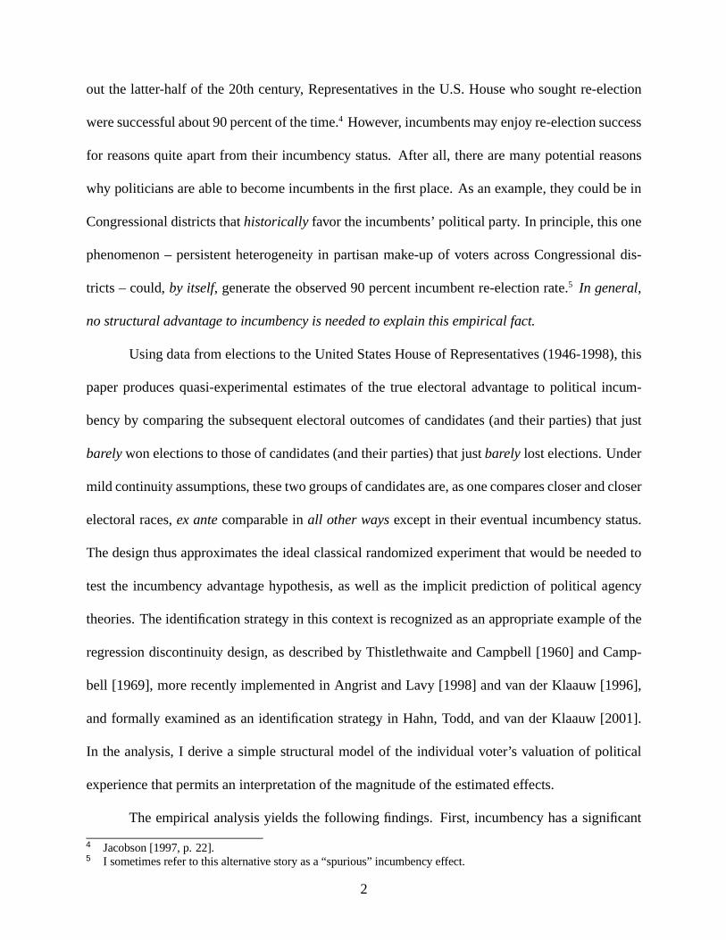
2 The Electoral Success of Incumbents - Advantage or Artifact?

For the U.S. House of Representatives, in any given election year, the incumbent party in

a given congressional district will likely win. The solid line in Figure I shows that this re-election

rate is about 90 percent and has been fairly stable over the past 50 years.6 Well-known in the

political science literature, the electoral success of the incumbent party is also reflected in the

two-party vote share, which is about 60 to 70 percent during the same period.7

As might be expected, incumbent candidates also enjoy a high electoral success rate. Fig-

ure I shows that the winning candidate has typically had a 80 percent chance of both running for

re-election and winning the following election. This slightly lower, because the probability that an

incumbent will be a candidate in the next election is about 88 percent, and the probability of win-

ning, conditional on running for election is about 90 percent. By contrast, the runner-up candidate

typically had a 3 percent chance of becoming a candidate and winning the next election. The prob-

ability that the runner-up is even a candidate in the next election is about 20 percent throughout

this period.

The casual observer is tempted to take these figures as evidence that there is an electoral

advantage to incumbency – that winning has a causal influence on the probability that the candi-

date will continue to run for office and eventually be elected. However, the difference between the

subsequent electoral outcomes of the winning and runner-up candidates may be due, perhaps en-

tirely, by the fact that the these two groups of candidates are ex ante non-comparable in important

ways.

Table I illustrates the point empirically. The first row and column indicates that the winner

of any given election at time t (i.e. the incumbent for election t + 1) has about a 0.803 chance of

6 Calculated from data on historical election returns from ICPSR study 7757. See Data Appendix for details. Notethat the “incumbent party” is undefined for years that end with ‘2’ due to decennial congressional re-districting.7 See, for example, the overview in Jacobson [1997].

4

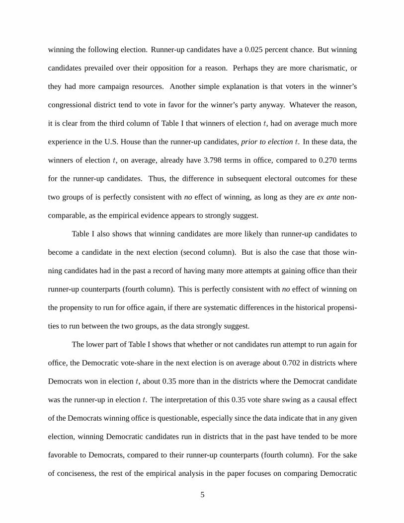
winning the following election. Runner-up candidates have a 0.025 percent chance. But winning

candidates prevailed over their opposition for a reason. Perhaps they are more charismatic, or

they had more campaign resources. Another simple explanation is that voters in the winner’s

congressional district tend to vote in favor for the winner’s party anyway. Whatever the reason,

it is clear from the third column of Table I that winners of election t, had on average much more

experience in the U.S. House than the runner-up candidates, prior to election t. In these data, the

winners of election t, on average, already have 3.798 terms in office, compared to 0.270 terms

for the runner-up candidates. Thus, the difference in subsequent electoral outcomes for these

two groups of is perfectly consistent with no effect of winning, as long as they are ex ante non-

comparable, as the empirical evidence appears to strongly suggest.

Table I also shows that winning candidates are more likely than runner-up candidates to

become a candidate in the next election (second column). But is also the case that those win-

ning candidates had in the past a record of having many more attempts at gaining office than their

runner-up counterparts (fourth column). This is perfectly consistent with no effect of winning on

the propensity to run for office again, if there are systematic differences in the historical propensi-

ties to run between the two groups, as the data strongly suggest.

The lower part of Table I shows that whether or not candidates run attempt to run again for

office, the Democratic vote-share in the next election is on average about 0.702 in districts where

Democrats won in election t, about 0.35 more than in the districts where the Democrat candidate

was the runner-up in election t. The interpretation of this 0.35 vote share swing as a causal effect

of the Democrats winning office is questionable, especially since the data indicate that in any given

election, winning Democratic candidates run in districts that in the past have tended to be more

favorable to Democrats, compared to their runner-up counterparts (fourth column). For the sake

of conciseness, the rest of the empirical analysis in the paper focuses on comparing Democratic

5

winning candidates to Democratic losing candidates.8

This paper proposes examining the data in a way that can distinguish between the proposed

causal effect of incumbency and the artifact of pure selection. Even though winning and losing

candidates are likely to be in general ex ante non-comparable, it is highly plausible that winners

of elections who win by a very slim margin are likely to be ex ante comparable to candidates who

barely lose the election by a very slim margin. In the extreme, among all political elections that

are decided by 1 vote, on average, the winners and the losers of those elections are almost certain

to be on average comparable. In practice, virtually no elections are decided by one vote. However,

under mild continuity and smoothness conditions, it is possible use data from elections within a

close neighborhood of this extreme case to estimate subsequent electoral outcomes of bare winners

and losers.9 The idea of exploiting cases when a treatment variable is a deterministic function of

an observed variable to credibly estimate causal effects originates in Thistlethwaite and Campbell

[1960]. Here, the nature of an election (the candidate of with the most votes wins, and becomes

the incumbent) is the deterministic function, and the observed variable is the vote share.

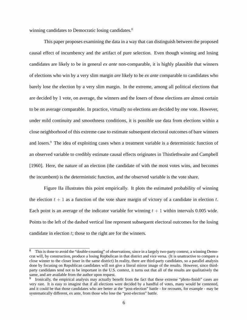
Figure IIa illustrates this point empirically. It plots the estimated probability of winning

the election t + 1 as a function of the vote share margin of victory of a candidate in election t.

Each point is an average of the indicator variable for winning t + 1 within intervals 0.005 wide.

Points to the left of the dashed vertical line represent subsequent electoral outcomes for the losing

candidate in election t; those to the right are for the winners.

8 This is done to avoid the “double-counting” of observations, since in a largely two-party context, a winning Demo-crat will, by construction, produce a losing Repbulican in that district and vice versa. (It is unattractive to compare aclose winner to the closer loser in the same district) In reality, there are third-party candidates, so a parallel analysisdone by focusing on Republican candidates will not give a literal mirror image of the results. However, since third-party candidates tend not to be important in the U.S. context, it turns out that all of the results are qualitatively thesame, and are available from the author upon request.9 Ironically, the empirical analysis may actually benefit from the fact that these extreme “photo-finish” cases arevery rare. It is easy to imagine that if all elections were decided by a handful of votes, many would be contested,and it could be that those candidates who are better at the “post-election” battle - for recounts, for example - may besystematically different, ex ante, from those who lose the “post-election” battle.

6

As apparent from the figure, there is a striking discontinuous jump, right at the 0 point,

indicating that bare winners of elections are much more likely to run for office and win the next

election than the bare losers. The effect is enormous: about 0.45 in probability. It is important to

note that nowhere else does a jump seem apparent. The data exhibit a well-behaved continuous

and smooth relationship between the two variables, except at the threshold that determines victory

and defeat.

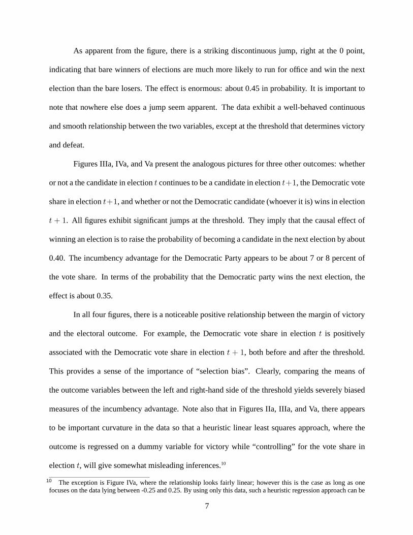
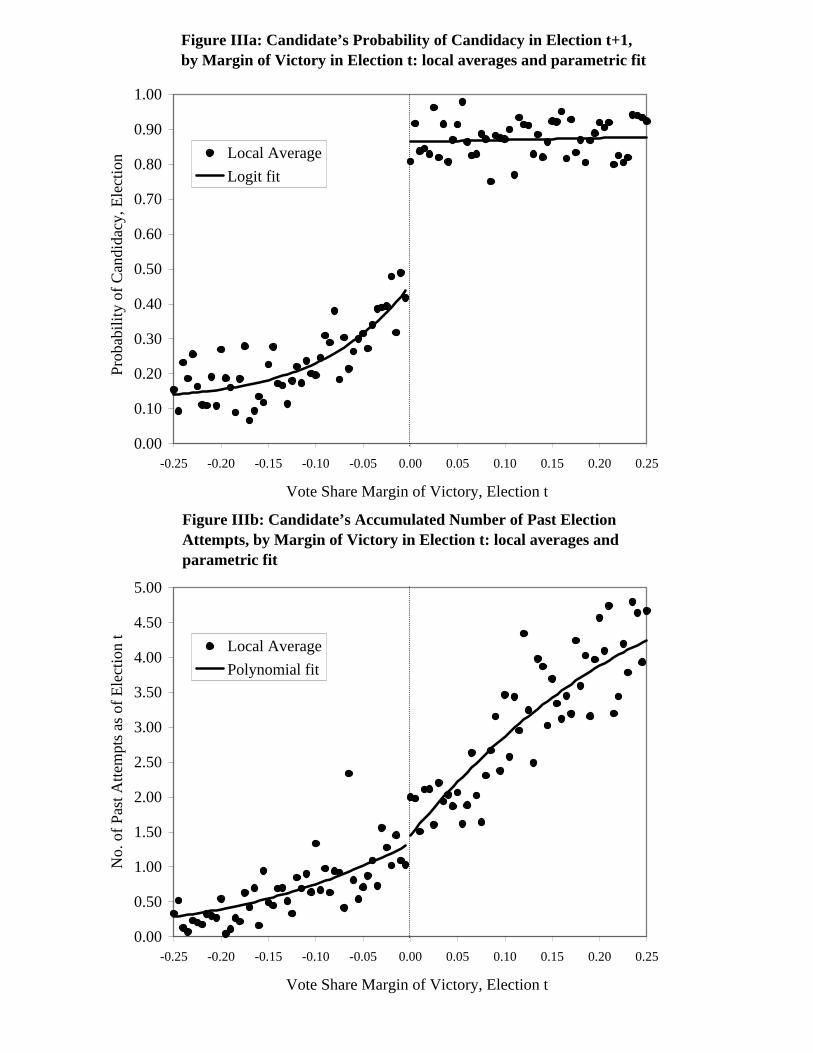
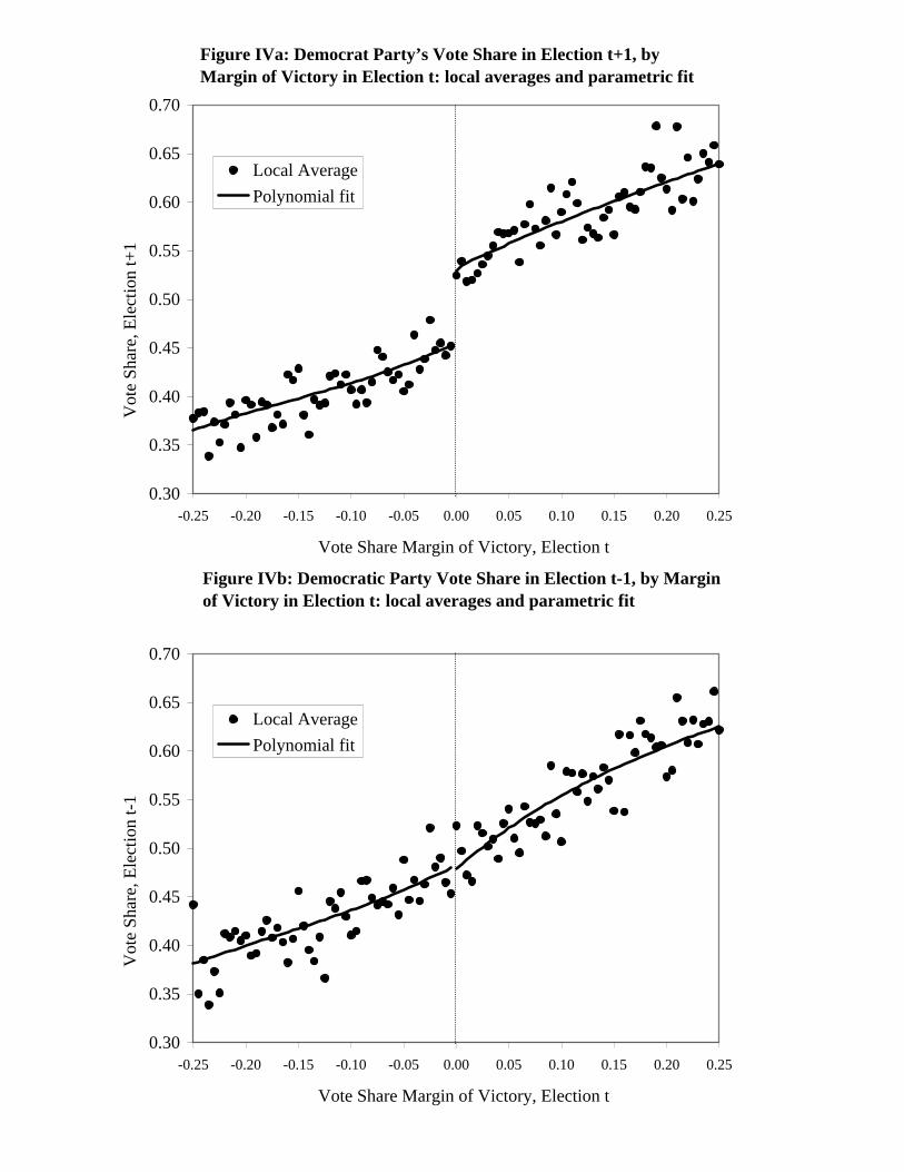
Figures IIIa, IVa, and Va present the analogous pictures for three other outcomes: whether

or not a the candidate in election t continues to be a candidate in election t+1, the Democratic vote

share in election t+1, and whether or not the Democratic candidate (whoever it is) wins in election

t + 1. All figures exhibit significant jumps at the threshold. They imply that the causal effect of

winning an election is to raise the probability of becoming a candidate in the next election by about

0.40. The incumbency advantage for the Democratic Party appears to be about 7 or 8 percent of

the vote share. In terms of the probability that the Democratic party wins the next election, the

effect is about 0.35.

In all four figures, there is a noticeable positive relationship between the margin of victory

and the electoral outcome. For example, the Democratic vote share in election t is positively

associated with the Democratic vote share in election t + 1, both before and after the threshold.

This provides a sense of the importance of “selection bias”. Clearly, comparing the means of

the outcome variables between the left and right-hand side of the threshold yields severely biased

measures of the incumbency advantage. Note also that in Figures IIa, IIIa, and Va, there appears

to be important curvature in the data so that a heuristic linear least squares approach, where the

outcome is regressed on a dummy variable for victory while “controlling” for the vote share in

election t, will give somewhat misleading inferences.10

10 The exception is Figure IVa, where the relationship looks fairly linear; however this is the case as long as onefocuses on the data lying between -0.25 and 0.25. By using only this data, such a heuristic regression approach can be

7

The identification strategy here crucially relies on the comparability of candidates and their

parties within a small neighborhood of either side of the 0 threshold. The credibility of the causal

inferences made here depend on this. Thus, it is instructive to examine the pre-determined char-

acteristics (outcomes that occur prior to election t) between the bare winners and losers. The

regression discontinuity design here has the very strong prediction that any such pre-determined

characteristics must not be systematically different between the bare winners and losers of elec-

tions. The extent to which they do differ is the extent to which we should place some doubt on

the internal validity of the research design. Such a prediction is analogous to the strong prediction

of an experiment that randomizes treatment and control, that the baseline characteristics of the

experimental subjects should not be in any ex ante observable way, systematically different from

the control subjects.

Figures IIb, IIIb, IVb, and Vb demonstrate that the data fail to reject the strong empirical

predictions of this research design. There is a strong positive relationship between the margin of

victory in election t and 1) past political experience, 2) electoral experience (the number of times

the candidate has run for election in the past), 3) the Democratic vote share in t−1, and 4) whether

the Democratic party won election t−1. However, Figure IIb shows, for example, that bare winners

and losers have, on average the same amount of accumulated congressional experience by time t.

There are also no visible discontinuities at the threshold for electoral experience, the previous

Democratic vote share or previous victory indicator. Close winners and losers do appear to be

quite comparable along these four dimensions; these facts lend credibility to the identification

strategy employed in this study.

thought of as a non-parmaeteric local linear estimate of the gap using a bandwidth of 0.50.

8

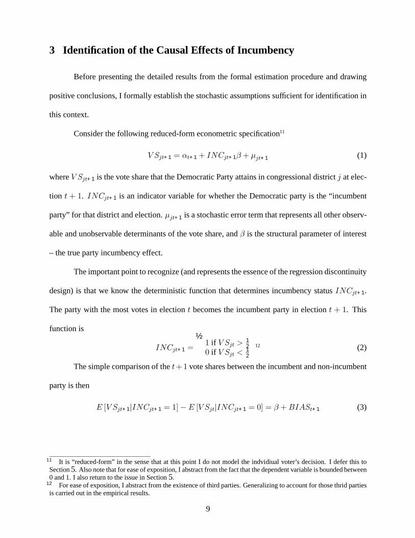
3 Identification of the Causal Effects of Incumbency

Before presenting the detailed results from the formal estimation procedure and drawing

positive conclusions, I formally establish the stochastic assumptions sufficient for identification in

this context.

Consider the following reduced-form econometric specification11

V Sjt+1 = αt+1 + INCjt+1β + µjt+1 (1)

where V Sjt+1 is the vote share that the Democratic Party attains in congressional district j at elec-

tion t + 1. INCjt+1 is an indicator variable for whether the Democratic party is the “incumbent

party” for that district and election. µjt+1 is a stochastic error term that represents all other observ-

able and unobservable determinants of the vote share, and β is the structural parameter of interest

– the true party incumbency effect.

The important point to recognize (and represents the essence of the regression discontinuity

design) is that we know the deterministic function that determines incumbency status INCjt+1.

The party with the most votes in election t becomes the incumbent party in election t + 1. This

function is

INCjt+1 =

½1 if V Sjt > 1

20 if V Sjt < 1

2

12 (2)

The simple comparison of the t+1 vote shares between the incumbent and non-incumbent

party is then

E [V Sjt+1|INCjt+1 = 1]− E [V Sjt|INCjt+1 = 0] = β +BIASt+1 (3)

11 It is “reduced-form” in the sense that at this point I do not model the indvidiual voter’s decision. I defer this toSection 5. Also note that for ease of exposition, I abstract from the fact that the dependent variable is bounded between0 and 1. I also return to the issue in Section 5.

12 For ease of exposition, I abstract from the existence of third parties. Generalizing to account for those thrid partiesis carried out in the empirical results.

9

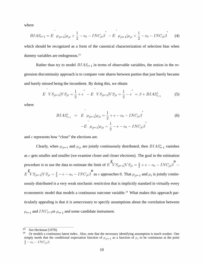
where

BIASt+1 = E

·µjt+1|µjt >

1

2− αt − INCjtβ

¸−E

·µjt+1|µjt <

1

2− αt − INCjtβ

¸(4)

which should be recognized as a form of the canonical characterization of selection bias when

dummy variables are endogenous.13

Rather than try to model BIASt+1 in terms of observable variables, the notion in the re-

gression discontinuity approach is to compare vote shares between parties that just barely became

and barely missed being the incumbent. By doing this, we obtain

E

·V Sjt+1|V Sjt = 1

2+ e

¸− E

·V Sjt+1|V Sjt = 1

2− e

¸= β +BIAS∗t+1

(5)

where

BIAS∗t+1= E

·µjt+1|µjt =

1

2+ e− αt − INCjtβ

¸(6)

−E·µjt+1|µjt =

1

2− e− αt − INCjtβ

¸and e represents how “close” the elections are.

Clearly, when µjt+1 and µjt are jointly continuously distributed, then BIAS∗t+1 vanishes

as e gets smaller and smaller (we examine closer and closer elections). The goal in the estimation

procedure is to use the data to estimate the limit of E£V Sjt+1|V Sjt = 1

2+ e− αt − INCjtβ

¤ −E

£V Sjt+1|V Sjt = 1

2− e− αt − INCjtβ

¤as e approaches 0. That µjt+1 and µt is jointly contin-

uously distributed is a very weak stochastic restriction that is implicitly standard in virtually every

econometric model that models a continuous outcome variable.14 What makes this approach par-

ticularly appealing is that it is unnecessary to specify assumptions about the correlation between

µt+1 and INCt+1or µt+1 and some candidate instrument.

13 See Heckman [1978].14 Or models a continuous latent index. Also, note that the necessary identifying assumption is much weaker. Onesimply needs that the conditional expectation function of µjt+1 as a function of µt to be continuous at the point12 − αt − INCjtβ.

10

4 Estimation of the Causal Effects of Incumbency

Table II illustrates that as one compares closer and closer elections, winning and losing

candidates look more similar, and suggests that the selection bias in the naive comparison of win-

ning and losing candidates can be quite large. In the first set of columns we see that the Democrats

obtain about 70 percent of the vote share in election t+ 1 when they win office in election t, com-

pared to about 35 percent of the vote when they lose. At the same time, on average, winning

candidates in any given election year typically have about 3.8 terms of congressional experience

and have run in about 4 elections prior to time t. Also note that the average political experience of

the winning Democrat candidate’s challenger (as of election t) is about 0.25 terms.15

The second set of columns demonstrate that the differences remain large when focusing

on the three-fourths of the sample in which the margin of victory is less than 50 percent of the

vote. The probability of Democrats winning election t + 1 remains large at 0.88 for winners in

t, compared to the 0.10 at t. And similarly, there remains a large difference, for example, in the

average electoral experience (the number of times a candidate has run in an election as of year t),

with a difference in favor of the winners of about 3.50 attempts.

A substantial portion of the differences go away when focusing on the 10 percent of the

elections that is decided by less than 5 percent of the vote, as shown in the third set of columns

in Table II. In this sample, the average difference in political and electoral experience between

the Democratic winners and losers is about 0.65 years, much smaller than in previous columns.

However, important differences persist: the winning Democrat candidate is significantly more

likely (by about 0.14 in probability) than a losing candidate to be in a district where the Democrats

had won the election in t−1. Moreover, all of the differences in the pre-determined characteristics

15 The “opposition” party is defined as the party (other than the Democrats) with the highest vote share in t − 1.Almost all of the time this is the Republican party.

11

(the variables in the 3rd through 8th rows) remain are statistically significant. It is important to

recognize, however, that this is to be expected: the sample average in a narrow neighborhood of

a margin of victory of 5 percent is in general a biased estimate of the true conditional expectation

function when that function has a nonzero slope (which it appears to have, as illustrated in Figures

II and III).

The approach in this paper is to estimate a flexible parameterization of the function leading

up to and after the threshold, in order to estimate the mean electoral outcome at the threshold

from the left and the right. For example, I regress the Democrat vote share t + 1 on a 4th-order

polynomial in the margin of victory in election t, separately, for the sample of winners in election t

(3818 observations) and for the sample of losing candidates at t (2740 observations). For indicator

variables, for example, whether or not the Democratic party won in t+ 1, I estimate a logit with a

4th order polynomial in the margin of victory, separately, for the winners and the losers.

Figures II, III, IV, and V all demonstrate that this procedure appears to visually perform

well. The regression and logit predictions do seem to line up well with the local averages plotted

in the figures. In particular, Figure IIIa suggests that the data asks for different kinds of curvature

on either side of the threshold.16

The final set of columns in Table II demonstrate that this procedure makes all of the dif-

ferences in the pre-determined characteristics between the winners and losers vanish, as exactly

predicted by the assumptions of the regression discontinuity design. In the third to eighth rows, all

16 In principle, it would be more attractive to view this as a nonparametric estimation problem, where the parameter ofinterest is the conditional expectation function just to the left and right of the threshold. It would also be more attractiveto utilize an automatic bandwidth selection procedure to determine the optimal amount of smoothing. However, eventhe so-called “automatic” data-based bandwidth selection procedure for the optimal (in the MSE sense) bandwidth at aparticular support of the regressor requires as an input an initial subjective smoothing parameter. See Fan and Gijbels[1996]. An assessment of the finite-sample performance of these procedures is beyond the scope of this study. Instead,I make that all of the functions belong to the class of fourth order polynomial (interacted with winner/loser) regressionequations and logits. Statistical inference is straightforward in this framework. It simply involves estimating thestandard error of parameteric predictions.

12

of the differences are small and statistically insignificant.17 By contrast, differences in the electoral

outcome variables – the Democrat vote share and actual whether they win in t+ 1 – remain large

and statistically significant. They imply a true electoral incumbency advantage of about 8 percent

in terms of the vote share, and about 0.36 in probability of winning election t+ 1.

If the bare winners and losers are in all other ways ex ante comparable near the discontinu-

ity threshold, then the estimated incumbency advantage is predicted to be invariant to the inclusion

(and in the way they enter) of pre-determined characteristics as covariates. Table III shows this

to be true: the results are quite robust to various specifications. Column (1) reports the estimated

incumbency effect on the vote share, when the vote share is regressed on the victory (in election t)

indicator, the quartic in the margin of victory, and their interactions. The estimate should and does

exactly match the differences in the first row of the last set of columns in Table II. Column (2) adds

to that regression the Democratic vote share and whether they won in t− 1. The Democratic share

in t− 1 comes in highly significant and statistically important. The coefficient on victory in t does

not change. The coefficient also does not change when the Democrat and opposition political and

electoral experience variables are included in Columns (2)-(5).

The estimated effect also remains stable when a completely different method of controlling

for pre-determined characteristics is utilized. In Column (6), the Democratic vote share t + 1

is regressed on all pre-determined characteristics (variables in rows three through eight), and the

discontinuity jump is estimated with the residuals of this first stage as the outcome variable. The

estimated incumbency advantage remains at about 8 percent of the vote share. Finally, in Column

(7) the vote share t− 1 is subtracted from the vote share in t+1 and the discontinuity jump in that

difference is examined. Again, the coefficient remains at about 8 percent.

Column (8) reports a final specification check of the regression discontinuity design and

17 This is favorable for the research design in the same way it would be comforting to see that the baseline character-istics between experimental and control subjects are on average the same in a classical randomized study.

13

estimation procedure. I attempt to estimate the causal effect of the impact of winning in election t

on the vote share in t − 1. Since we know that the outcome of election t cannot possibly causally

effect the electoral vote share in t−1, the estimated impact should be zero. If it significantly departs

from zero, this calls into question, some aspect of the identification strategy and/or estimation

procedure. The estimated effect is essentially 0, with a fairly small estimated standard error of

0.011. All specifications in Table III were repeated for the indicator variable for a Democrat victory

in t+ 1 as the dependent variable, and the estimated coefficient was stable across specifications at

about 0.38 and it passed the specification check of Column (8) with a coefficient of -0.005 with a

standard error of 0.033.

By way of summarizing the results, Table IV reports the estimated causal effects of incum-

bency using the three other outcome measures that were examined in Figures IIa, IIIa, IVa, and

Va. All estimates use the full specification of Column (5) in Table III. The first two entries in the

top panel show that, at the individual candidate level, winning an election increases the probabil-

ity that the candidate will run for office again and be successful by about 0.45 in probability. It

increases the probability of becoming a candidate in the next election by about 0.434. It is impor-

tant to emphasize that these are not simple associational correlations. They represent the kind of

causal effects – quite plausibly free of unobservable selection bias – that can strongly suggest that

there losing may have a real deterrence effect on the decision to run for office.18 If the politician

is making an expected utility calculation, this suggests that there is strong empirical evidence that

either the perceived payoffs or probabilities of winning (or both) shift against the runner-up quite

significantly.

It is also important to note that since losing has an enormous impact on even attempting

to run for office, it will be virtually impossible to convincingly estimate the candidate-level in-

18 Such a possible deterrent effect is discussed in Levitt and Wolfram [1997].

14

cumbency advantage in terms of the vote share advantage for the individual candidates, without

imposing a great deal of structure on the unobservable process that determines the candidate’s

decision to run for office.19 This is because we will never observe the vote share for candidates

who choose not to pursue elected office. This is analogous to the inherent difficulty in estimating

a treatment effect in a classical randomized experiment when most of the controls drop out of the

sample.

On the other hand, the true incumbency advantage for the party in a congressional district

is well-defined, because typically some other candidate will replace any past challengers who drop

out of politics.20 The third and fourth entries in the top panel of Table IV indicate that the causal

effect of the Democrat winning office is to raise the Democrat vote share by 0.078 in the next

election, and raise the probability that the Democratic candidate will win by 0.385.

The results make clear that the electoral success of incumbents is not an artifact of se-

lection, and hence the evidence is at least broadly consistent with the reduced-form prediction of

many political agency hypotheses that incumbents successfully utilize the opportunities embodied

in elected office to be re-elected.21

Finally, the lower panel of Table IV shows that there is little evidence that these estimated

incumbency effects vary by sub-groups defined by the amount of political experience that the

candidate possess at election t. It would be interesting to know if the incumbency advantage

diminishes or increases as we consider more and more experienced candidates. For example, a

finding that the incumbency advantage disappeared when considering candidates that have already

19 For the approaches that attempt to tackle this difficult issue, refer to the sample selection literature beginning withe.g. Heckman [1979] and Gronau [1977].

20 And even in the case where no candidate runs for the party, it is not unreasonable to assign “0” to the vote shareattained by the party in that district and year.

21 Strictly speaking, political agency theories have yet to explicitly model the dynamic of how a candidate within aparty is chosen, and how candidates decide to run with the expectation of how the party will support them. However,ignoring those inter-party dynamics, the “agent” could be heuristically defined as the set of possible candidates for aparty within a congressional district, where the party in power pursues actions that are implicitly rewarded by voters.

15

been in office for a number of terms would be consistent with the notion of a signaling mechanism

[Rogoff 1990], where incumbents pursue policies to signal their type (good or bad) to voters.

However, the results are somewhat mixed. While the point estimates of the incumbency effects do

appear smaller for more experienced candidates in three of the four electoral outcome measures,

it is also true that the F-test in each case fails to reject equality of the coefficients across these

sub-groups. This suggests that any empirical analysis that purports to sort out these second order

effects will require much more data than that used in this analysis.

5 An Econometric Model of Voters’ Implicit Valuation of PoliticalExperience

In this section I develop a simple structural model of individual voting behavior for the pur-

pose of providing an economic interpretation of the magnitudes of the estimates of the incumbency

advantage.

The analysis thus far has addressed the first-order, difficult issue of disentangling a true

electoral return to holding office from an obscuring unobservable selection process. Possessing

arguably credible estimates of this incumbency advantage is a first step towards deepening our

understanding of underlying voter preferences. Given that the findings are broadly consistent with

the implications of political agency theories, it will be a fruitful avenue for research to subject these

various theories to further empirical tests – while simultaneously addressing important selection

issues that typically make it difficult to distinguish between association and causation. This will re-

quire detailed, data on measurable politician actions: ultimately we cannot empirically distinguish

between various hypothesized mechanisms of political agency with election returns data alone.

Nonetheless, the reduced-form estimates from these election returns data do suggest that

voters place some value on incumbency, when deciding for whom to vote. It is thus useful to

16

explore what kind of institutional and behavioral assumptions we can impose on the data in the

present study, in order to make a statement about the nature of voter preferences within an eco-

nomic model of utility-maximizing voters.

Many of the assumptions of the model are motivated by the limitations of the data used in

this empirical study. The distinctive features of the model are: 1) the politician action set is not at

the individual congressional district level, but at the national (two-party) level; in each election t,

there is a national party “platform” to which the candidates of each party uniformly adhere, and 2)

citizens have heterogeneous political preferences, but make their decision based on two factors: the

national party platforms, and the relative political experience of the two candidates, independent

of their party affiliation.

The model yields an intuitive empirical implication. Dividing the causal effect of a Demo-

cratic win in t on (a monotonic transformation of) the vote share in t+ 1, by the causal effect of a

Democratic win in t on the Democratic experience advantage in t+ 1 yields the voter’s valuation

of an additional congressional term of politician experience.

Suppose that in any congressional district j at election t + 1, we can represent individual

voter i’s political preference by the scalar εijt+1; higher εijt+1represents more liberal preferences.

It is taken as primitive (exogenous), with εijt+1 ∼ N (ajt+1, 1) , so that preferences are heteroge-

neous within district and year, but the location of the distribution varies arbitrarily across districts

and over time. Assume a two-party system, and that in any given election year t+1 the Democratic

platform is represented by the scalar δt+1 and the Republican platform by ρt+1, with δt+1 > ρt+1.

Since we have no data on the process that generates δt+1 or ρt+1, I treat it as an unobservable pro-

cess. However, I do assume that no single Congressional district electoral outcome can influence

the national party platform. This is an important assumption of the structural model.

Finally, assume that citizens’s voting is influenced by two factors: 1) the relative “close-

17

ness” of the national party platforms to their own political preferences, and 2) the relative Con-

gressional experience ∆EXPjt+1 (normalized as the Democrat’s political experience minus that

of the Republican, and measured in number of Congressional terms) of the two candidates.

The vote vijt+1 of individual i in district j at election t+ 1 is thus described by

vijt+1 =

½Democrat if |εijt+1 + γ∆EXPjt+1 − δt+1| <

¯̄εijt+1 + γ∆EXPjt+1 − ρt+1

¯̄Republican otherwise (7)

with the value of candidates’ Congressional experience denoted by γ, γ > 0. So, for example, if

there is no political experience difference between the two candidates, voters will choose based

on the national party platform alone. But if ∆EXPjt+1 > 0 (the Democratic candidate is more

experienced), then individuals may vote for the Democrat candidate, even though their positions

are closer to the Republican national platform. The reverse is true for∆EXPjt+1 < 0.

This voting rule is equivalent to

vijt+1 =

½Democrat if εijt+1 >

δt+ρt

2− γ∆EXPjt+1

Republican otherwise (8)

which implies that the vote share obtained by the Democrat in district j at election t+ 1 is

V Sjt+1 = Φ (γ∆EXPjt+1 + θjt+1) (9)

where θjt+1 = −δt+ρt

2+ ajt+1. V Sjt+1 is directly observed in the available election return data.

The inverse normal cdf transformation of the data

Φ−1jt+1 = Φ

−1 (V Sjt+1) = γ∆EXPjt+1 + θjt+1 (10)

is also observable.

No assumptions are made about the process that determines ∆EXPjt, except that past

electoral outcomes may play at least some role. We can always write

∆EXPjt+1 = f (V Sjt) + ujt+1 (11)

18

with ujt+1 is defined as∆EXPjt+1 − f (V Sjt), where

f (V Sjt) =

½∆EXPjt + 1 if V Sjt > 1

2∆EXPjt − 1 if V Sjt < 1

2

(12)

If all candidates always choose to run for office in the same district regardless of past electoral

outcomes, then ujt+1 is always 0. In other words, if the Democrat wins in election t, he will have

an experience advantage of 1 year in election t + 1, but if he loses, he will have an experience

disadvantage of 1 year. More generally, candidates do drop out of politics, and this generates the

error ujt+1, which can in general be correlated with θjt+1. Whether the outcome of election t

influences ∆EXPjt+1 is, of course, ultimately an empirical question.

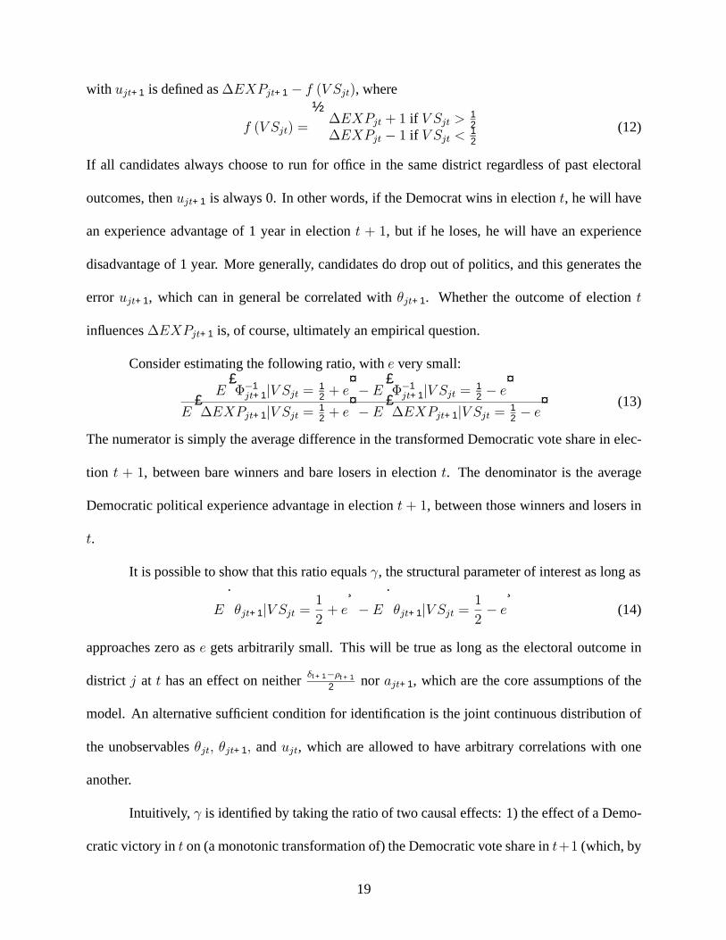
Consider estimating the following ratio, with e very small:

E£Φ−1jt+1|V Sjt = 1

2+ e

¤− E £Φ−1jt+1|V Sjt = 1

2− e¤

E£∆EXPjt+1|V Sjt = 1

2+ e

¤− E £∆EXPjt+1|V Sjt = 1

2− e¤ (13)

The numerator is simply the average difference in the transformed Democratic vote share in elec-

tion t + 1, between bare winners and bare losers in election t. The denominator is the average

Democratic political experience advantage in election t + 1, between those winners and losers in

t.

It is possible to show that this ratio equals γ, the structural parameter of interest as long as

E

·θjt+1|V Sjt = 1

2+ e

¸− E

·θjt+1|V Sjt = 1

2− e

¸(14)

approaches zero as e gets arbitrarily small. This will be true as long as the electoral outcome in

district j at t has an effect on neither δt+1−ρt+1

2nor ajt+1, which are the core assumptions of the

model. An alternative sufficient condition for identification is the joint continuous distribution of

the unobservables θjt, θjt+1, and ujt, which are allowed to have arbitrary correlations with one

another.

Intuitively, γ is identified by taking the ratio of two causal effects: 1) the effect of a Demo-

cratic victory in t on (a monotonic transformation of) the Democratic vote share in t+1 (which, by

19

assumption, operates through the voters’ valuation of experience) and 2) the effect of a Democratic

victory in t on the Democratic experience advantage in election t+ 1. Each of these causal effects

can be estimated using the same procedure described in Section 4.

6 Structural Estimates and Alternative Estimation Approaches

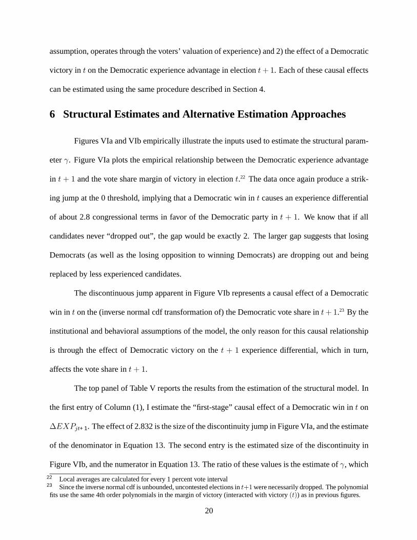
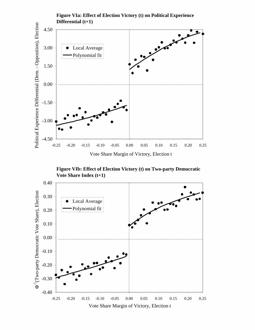
Figures VIa and VIb empirically illustrate the inputs used to estimate the structural param-

eter γ. Figure VIa plots the empirical relationship between the Democratic experience advantage

in t + 1 and the vote share margin of victory in election t.22 The data once again produce a strik-

ing jump at the 0 threshold, implying that a Democratic win in t causes an experience differential

of about 2.8 congressional terms in favor of the Democratic party in t + 1. We know that if all

candidates never “dropped out”, the gap would be exactly 2. The larger gap suggests that losing

Democrats (as well as the losing opposition to winning Democrats) are dropping out and being

replaced by less experienced candidates.

The discontinuous jump apparent in Figure VIb represents a causal effect of a Democratic

win in t on the (inverse normal cdf transformation of) the Democratic vote share in t+ 1.23 By the

institutional and behavioral assumptions of the model, the only reason for this causal relationship

is through the effect of Democratic victory on the t + 1 experience differential, which in turn,

affects the vote share in t+ 1.

The top panel of Table V reports the results from the estimation of the structural model. In

the first entry of Column (1), I estimate the “first-stage” causal effect of a Democratic win in t on

∆EXPjt+1. The effect of 2.832 is the size of the discontinuity jump in Figure VIa, and the estimate

of the denominator in Equation 13. The second entry is the estimated size of the discontinuity in

Figure VIb, and the numerator in Equation 13. The ratio of these values is the estimate of γ, which22 Local averages are calculated for every 1 percent vote interval23 Since the inverse normal cdf is unbounded, uncontested elections in t+1were necessarily dropped. The polynomialfits use the same 4th order polynomials in the margin of victory (interacted with victory (t)) as in previous figures.

20

is 0.073, highly statistically significant.24 This estimate implies that an additional Congressional

term of experience (above the opposite candidate) attracts voters towards that candidate by 0.073

of a standard deviation (in terms of underlying political preferences within a district), a seemingly

modest magnitude. However, in close elections, that 0.073 translates to a 2.5 percent vote share

difference, which of course can make a significant influence on the eventual outcome.

The deceptively small estimate of γ can play a significant role accounting for the persis-

tently high electoral success of incumbents in the U.S. House. I use my estimate of γ to ask what

would the incumbent party re-election rate be if all ∆EXPjt+1 were set to zero. This would cor-

respond to the extreme policy of mandatory term limits of 1, where in each election, no candidate

has an experience advantage. Adjusting the actual vote shares by bγ∆EXPjt+1 and tallying up

the counterfactual electoral outcomes yields a dramatic impact. The electoral success the incum-

bent party falls from about 90 percent to 60 percent, and the electoral success of the non-incumbent

party rises from about 10 percent to 40 percent. Approximately two-thirds of the observed electoral

success can be explained by the existing distribution of experience differences between candidates

for the U.S. House. This makes some intuitive sense, since we know (Table II) that the average

political experience difference is more than 3 and half terms of experience. The average difference

between the simulated and actual vote shares is about 10 percent, a significant political magnitude.

Finally, the bottom panel of Table V reports the estimates of the structural parameter un-

der alternative specifications: a heuristic “fixed effects” and an alternative “instrumental variable”

approach to modeling the unobservables. An attractive feature of a research design where there is

arguably not only exogenous but also (as good as) random variation in the “treatment” variable,

is that it provides a baseline for assessing whether or not other commonly-used econometric ap-

24 Practically, this is an instrumental variable estimate from regression of the transformed vote share on∆EXPjt+1

instrumenting with the indicator of a Democratic win in t, using the 4th order polynomial in the margin of the victory(and the interaction of these terms with the win indicator) as covariates.

21

proaches would yield the same “experimental” estimate.25 Since “fixed effects” and “instrumental

variable” approaches implicitly assume continuity of the distribution of unobservables, the typical

assumptions used in “differencing” and IV approaches are necessarily more restrictive than the

mild stochastic assumptions invoked in Section 5. Thus, substantial deviation of the alternative

specifications from the baseline results of Table V would be an indication that the assumptions

required for “fixed effects” and other “IV” approaches are invalid in this particular context.

Table V show that these estimates indeed depart substantially from the quasi-experimental

estimates. The estimates of a “fixed-effect” regression yields an estimate of 0.022, which is less

than a third of the magnitude of the baseline regression discontinuity estimate of γ.26 The fixed

effects assumption appears to be inappropriate in this context.

Suppose the econometrician were to utilize the assumed exclusion restriction that a Demo-

cratic victory does not directly and independently impact the electoral outcome in t + 1 except

through ∆EXPjt+1. But suppose the analyst were to conjecture that there was “no reason to

believe that a Democratic victory should be correlated with θjt+1.”27 These assumptions would

suggest an IV estimator that does not control for a non-parametric function of the margin of vic-

tory at t.28 This analyst would obtain misleading inferences regarding γ, as shown by the last row

of estimates in Table V. This IV approach is yields estimates that are about 50 percent too high.

In this particular application, the best estimate is in fact the simplest cross-sectional OLS

25 This is the spirit of the influential work of Lalonde [1986]. Obviously, the situation here is not literally a controlled,true “experiment”. However, in a sense, there is as much evidence that this is as good as a randomized experimentas there is, for example, that the NSW program was correctly randomized in Lalonde [1986]. This was the point ofshowing Table II, which is analogous to Lalonde’s Table I that provides empirical evidence that the randomization“worked”.

26 This “differencing” specification is a regression of the the transformed vote share on a set of year dummies (topresumably “absorb” the δt−ρt

2 term), state-district-decade dummies (that presumably “absorbs” the “permanent het-erogeneity” in ajt; i.e. the assumption is that ajt0 = ajt00 for all t0 and t00 within a decade), and∆EXPjt+1.

27 Actually, given the setup of the model, there are a lot of reasons to expect that the Democrat win variable shouldbe correlated with θjt+1. Namely, a simple autocorrelation of ajt would produce such a correlation.

28 Specifically, the regression is the transformed vote share on ∆EXPjt+1 using the Democratic victory indicatorfor t as an instrument, and including year dummies as the covariates.

22

regression, which yields an estimate of about 0.06 for γ.29 On the other hand, both the OLS and

alternative IV estimates give misleading inferences concerning whether γ varies by sub-groups

defined by ∆EXPjt. They imply that the γ declines with a higher initial ∆EXPjt, when in fact,

as the top panel of Table V demonstrates, the interaction effects are statistically insignificant. The

null hypothesis of homogeneity along this dimension cannot be rejected.

7 Conclusions

This paper exploits the “near”-random assignment of incumbency generated by close U.S.

House elections in order to 1) assess whether or not the electoral success of incumbents is a mere

artifact of selection, 2) quantify the reduced-form causal relationship of incumbency on subse-

quent electoral outcomes, 3) provide an input – arguably free of selection bias – to a structural

model of voting behavior that produces an estimate of the voter’s valuation of political experience,

and 4) to evaluate the performance of commonly-used alternative approaches to modelling the

unobservables within this empirical example.

I find evidence that rejects the pure spurious-selection hypothesis, and estimate that incum-

bency has a significant positive causal effect on the probability that the incumbent candidate or

party will run again for office and succeed, by about 0.40 to 0.45. Losing candidates most often do

not run again for election, and while much of this is due to selection, a significant portion of this

represents a causal relationship. A structural model implies that heterogeneity in political prefer-

ences across voters (within district) is quite large, relative to the implicit valuation of congressional

experience, but that even this modest valuation can be important. According to the model, about

two-thirds of the apparent electoral success of incumbents can be attributed to the distribution of

political experience differences across Congressional districts in the U.S. Finally, the results sug-

29 The specification is a regression of the transformed vote share on∆EXPjt+1 and a set of year dummies.

23

gest that an analyst relying on a “fixed effect” approach to estimating the valuation of experience

would obtain a significantly downward-biased estimated. They also suggest that an analyst em-

ploying “IV” by relying on the assumed exclusion restriction – but simply asserting orthogonality

of the instrument and the unobservable error term – would generate seriously upwardly-biased

estimates in this particular context.

Meaningful theories of political agency ultimately make causal empirical predictions. If

there is any hope in assessing whether any or which of these theories have empirical relevance,

it lies in evaluating whether or not there is definitive evidence that these causal relationships ap-

pear in real-world data. Unobservable selection and omitted-variable bias is endemic in empirical

research, so such definitive evidence is likely to be quite rare; unilaterally relying on a particular

approach (e.g. “differencing” or “IV”) for modelling unobservable mechanisms has the potential to

produce misleading inferences. On the other hand, it appears that examining the “near”-experiment

generated by close elections may be a promising approach in this line of research.

24

Data Appendix

The data used for this analysis is based on the candidate-level Congressional election returns for the

U.S., from ICPSR study 7757, “Candidate and Constituency Statistics of Elections in the United

States, 1788-1990”.

The data were intially checked for internal consistencies (e.g. candidates’ vote totals not

equalling reported total vote cast), and corrected using published and official sources (Congres-

sional Quartlery [1997] and the United States House of Representatives Office of the Clerk’s Web

Page). Election returns from 1992-1998 were taken from the United States House of Representa-

tives Office of the Clerk’s Web Page, and appended to these data. Various states (e.g. Arkansas,

Louisiana, Florida, and Oklahoma) have laws that do not require the reporting of candidate vote

totals if the candidate ran unopposed. If they are the only candidate in the district, they were as-

signed a vote share of 1. Other individual missing vote totals were replaced with valid totals from

published and official sources. Individuals with more than one observation in a district year (e.g.

separate Liberal and Democrat vote totals for the same person in New York and Connecticut) were

given the total of the votes, and was assigned to the party that gave the candidate the most votes.

The name of the candidate was parsed into last name, first name, and middle names, and suffixes

such as “Jr., Sr., II, III, etc.”

Since the exact spelling of the name differs across years, the following algorithm was used

create a unique identifier for an individual that could match the person over time. Individiuals

were first matched on state, first 5 characters of the last name, and first initial of the first name. The

second layer of the matching process isolates those with a suffix such as Jr. or Sr., and small number

of cases were hand-modified using published and official sources. This algorithm was checked by

drawing a random sample of 100 election-year-candidate observations from the original sample,

25

tracking down every separate election the individual ran in (using published and official sources;

this expanded the random sample to 517 election-year-candidate observations), and asking how

well the automatic algorithm performed. The fraction of observations from this “truth” sample

that matched with the processed data was 0.982. The fraction of the processed data for which there

was a “true” match was 0.992. Many different algorithms were tried, but the algorithm above

performed best based on the random sample.

Throughout the sample period (1946-1998), in about 3 percent of the total possible number

of elections (based on the number of seats in the House in each year), no candidate was reported

for the election. I impute the missing values using the following algorithm. Assign the state-year

average electoral outcome; if still missing, assign the state-decade average electoral outcome.

Two main data sets are constructed for the analysis. For all analysis at the Congressional

level, I keep all years that do not end in ‘0’ or ‘2’. This is because, strictly speaking, Congressional

districts cannot be matched between those years, due to decennial re-districting, and so in those

years, the previous or next electoral outcome is undefined. The final data set has 6558 observations.

For the analysis at the individual candidate level, one can use more years, because, despite re-

districting, it is still possible to know if a candidate ran in some election, as well as the outcome.

This larger dataset has 9674 Democrat observations.

For the sake of conciseness, the the empirical analysis in the paper focuses on observations

for Democrats only. This is done to avoid the “double-counting” of observations, since in a largely

two-party context, a winning Democrat will, by construction, produce a losing Repbulican in that

district and vice versa. (It is unattractive to compare a close winner to the closer loser in the

same district) In reality, there are third-party candidates, so a parallel analysis done by focusing

on Republican candidates will not give a literal mirror image of the results. However, since third-

party candidates tend not to be important in the U.S. context, it turns out that all of the results are

26

qualitatively the same, and are available from the author upon request.

27

References[1] Alesina, Alberto, and Howard Rosenthal. “Partisan Cycles in Congressional Elections and the

Macroeconomy.” American Political Science Review 83 (1989): 373-398.[2] Alford, John R., and John R. Hibbing. “Increased Incumbency Advantage in the House.”

Journal of Politics 43 (1981): 1042-61.[3] Angrist, Joshua D., and Victor Lavy. “Using Maimondies’ Rule to Estimate the Effect of Class

Size on Scholastic Achievement.” Quarterly Journal of Economics 114 (1998):533-75.[4] Baron, David P. “Service-induced Campaign Contributions and the Electoral Equilibrium.”

Quarterly Journal of Economics 104 (1989): 45-72.[5] Besley Timothy, and Anne Case. “Does Electoral Accountability Affect Economic Policy

Choices? Evidence from Gubernatorial Term Limits.” Quarterly Journal of Economics 110(1995): 769-798.

[6] Besley Timothy, and Anne Case. “Incumbent Behavior: Vote-Seeking, Tax-Setting, and Yard-stick Competition.” American Economic Review 85 (1995): 25-45.

[7] Campbell, D. T. “Reforms as Experiments.” American Psychologist 24 (1969): 409-29.[8] Collie, Melissa P. “Incumbency, Electoral Safety, and Turnover in the House of Representa-

tives, 1952-1976.” American Political Science Review 75 (1981): 119-31.[9] Congressional Quartlery. Congressional Elections: 1946-1996. 1997.[10]Erikson, Robert S. “The Advantage of Incumbency in Congressional Elections.” Polity 3

(1971): 395-405.[11]Fan, J., and I. Gijbels. Local Polynomial Modelling and Its Applications, New York, New

York: Chapman and Hall, 1996.[12]Garand, James C., and Donald A. Gross. “Change in the Vote Margins for Congressional

Candidates: A Specification of the Historical Trends.” American Political Science Review 78(1984): 17-30.

[13]Gelman, Andrew, and Gary King. “Estimating Incumbency Advantage without Bias.” Ameri-can Journal of Political Science 34 (1990): 1142-64.

[14]Gronau, R. “Leisure, home production and work – the theory of the allocation of time revis-ited.” Journal of Political Economy 85 (1977): 1099-1124.

[15]Grossman Gene M., and Elhanan Helpman. “Electoral Competition and Special Interest Poli-tics.” Review of Economic Studies 63 (1996): 265-286.

[16]Hahn, Jinyong, Petra Todd, and Wilbert van der Klaauw. “Identification and Estimation ofTreatment Effects with a Regression-Discontinuity Design.” Econometrica 69 (2001): 201-209.

[17]Heckman, James J. “Dummy Endogenous Variables in a Simultaneous Equations System.”Econometrica 46 (1978): 931-59.

[18]Heckman, James J. “Sample selection bias as a specification error.” Econometrica 47 (1979):153-62.

[19] Inter-university Consortium for Political and Social Research. “Candidate and ConstituencyStatistics of Elections in the United States, 1788-1990” Computer File 5th ICPSR ed. AnnArbor, MI: Inter-university Consortium for Political and Social Research, producer and dis-tributor, 1995.

28

[20] Jacobson, Gary C. “The Marginals Never Vanished: Incumbency and Competition in Electionsto the U.S. House of Representatives.” American Journal of Political Science 31 (1987): 126-41.

[21] Jacobson, Gary C. The Politics of Congressional Elections, Menlo Park, California: Longman,1997.

[22]Kalt, Joseph P., and Mark A. Zupan. “Capture and Ideology in the Economic Theory of Poli-tics.” American Economic Review 74 (1984): 279-300.

[23]Lalonde, Robert J. “Evaluating the Econometric Evaluations of Training Programs with Ex-perimental Data.” American Economic Review 76 (1986): 604-620.

[24]Lee, David S. “Is there Really an Electoral Advantage to Incumbency?: Evidence from CloseElections to the United States House of Representatives.” mimeo, April, 2000.

[25]Levitt, Steven D. “Using Repeat Challengers to Estimate the Effect of Campaign Spending onElection Outcomes in the U.S. House.” Journal of Political Economy 102 (1994): 777-798.

[26]Levitt, Steven D., and James M. Poterba. “Congressional Distributive Politics and State Eco-nomic Performance.” NBER Working Paper #4721 (1994).

[27]Levitt, Steven D. “How Do Senators Vote? Disentangling the Role of Voter Preferences, PartyAffiliation, and Senator Ideology.” American Economic Review 86 (1996): 425-441.

[28]Levitt, Steven D., and Catherine D. Wolfram. “Decomposing the Sources of Incumbency Ad-vantage in the U.S. House.” Legislative Studies Quarterly 22 (1997) 45-60.

[29]Payne, James L. “The Personal Electoral Advantage of House Incumbents.” American PoliticsQuarterly 8 (1980): 375-98.

[30]Peltzman, Sam. “Constituent Interest and Congressional Voting.” Journal of Law and Eco-nomics 27 (1984): 181-210.

[31]Peltzman, Sam. “An Economic Interpretation of the History of Congressional Voting in theTwentieth Century.” American Economic Review 75 (1985): 656-675.

[32]Rogoff, Kenneth. “Equilibrium Political Budget Cycles.” American Economic Review 80 (1990):21-36.

[33]Rogoff, Kenneth, and Anne Sibert. “Elections and Macroeconomic Policy Cycles” Review ofEconomic Studies 55 (1988): 1-16.

[34]Snyder, James M. “Campaign Contributions as Investments: The U.S. House of Representa-tives, 1980-1986.” Journal of Political Economy 98 (1990): 1195-1227.

[35]Thistlethwaite, D., and D. Campbell. “Regression -Discontinuity Analysis: An alternative tothe ex post facto experiment.” Journal of Educational Psychology 51 (1960): 309-17.

[36]Van der Klaauw, Wilbert. “Estimating the Effect of Financial Aid Offers on College Enroll-ment: A Regression-Discontinuity Approach.” Unpublished manuscript (1996).

29

FIGURE I: Electoral Success of U.S. House Incumbents: 1948-1998

0

0.1

0.2

0.3

0.4

0.5

0.6

0.7

0.8

0.9

1

1948 1958 1968 1978 1988 1998

Year

Incumbent PartyWinning CandidateRunner-up Candidate

Prop

orti

on W

inni

ng E

lect

ion

Note: Calculated from ICPSR study 7757. Details in Data Appendix. Incumbent party is the party that won the electionin the preceding election in that congressional district. Due to re-districting on years that end with "2", there are nopoints on those years. Other series are the fraction of individual candidates in that year, who win an election in thefollowing period, for both winners and runner-up candidates of that year.

0.00

0.10

0.20

0.30

0.40

0.50

0.60

0.70

0.80

0.90

1.00

-0.25 -0.20 -0.15 -0.10 -0.05 0.00 0.05 0.10 0.15 0.20 0.25

Local Average

Logit fit

Vote Share Margin of Victory, Election t

Prob

abili

ty o

f W

inni

ng, E

lect

ion

t+1

Figure IIa: Candidate’s Probability of Winning Election t+1, by Margin of Victory in Election t: local averages and parametric fit

0.00

0.50

1.00

1.50

2.00

2.50

3.00

3.50

4.00

4.50

5.00

-0.25 -0.20 -0.15 -0.10 -0.05 0.00 0.05 0.10 0.15 0.20 0.25

Local Average

Polynomial fit

Vote Share Margin of Victory, Election t

No.

of

Past

Vic

tori

es a

s of

Ele

ctio

n t

Figure IIb: Candidate’s Accumulated Number of Past Election Victories, by Margin of Victory in Election t: local averages and parametric fit

0.00

0.10

0.20

0.30

0.40

0.50

0.60

0.70

0.80

0.90

1.00

-0.25 -0.20 -0.15 -0.10 -0.05 0.00 0.05 0.10 0.15 0.20 0.25

Local Average

Logit fit

Vote Share Margin of Victory, Election t

Prob

abili

ty o

f C

andi

dacy

, Ele

ctio

n

Figure IIIa: Candidate’s Probability of Candidacy in Election t+1, by Margin of Victory in Election t: local averages and parametric fit

0.00

0.50

1.00

1.50

2.00

2.50

3.00

3.50

4.00

4.50

5.00

-0.25 -0.20 -0.15 -0.10 -0.05 0.00 0.05 0.10 0.15 0.20 0.25

Local Average

Polynomial fit

Vote Share Margin of Victory, Election t

No.

of

Past

Atte

mpt

s as

of

Ele

ctio

n t

Figure IIIb: Candidate’s Accumulated Number of Past Election Attempts, by Margin of Victory in Election t: local averages and parametric fit

0.30

0.35

0.40

0.45

0.50

0.55

0.60

0.65

0.70

-0.25 -0.20 -0.15 -0.10 -0.05 0.00 0.05 0.10 0.15 0.20 0.25

Local Average

Polynomial fit

Vote Share Margin of Victory, Election t

Vot

e S

hare

, Ele

ctio

n t+

1

Figure IVa: Democrat Party’s Vote Share in Election t+1, by Margin of Victory in Election t: local averages and parametric fit

0.30

0.35

0.40

0.45

0.50

0.55

0.60

0.65

0.70

-0.25 -0.20 -0.15 -0.10 -0.05 0.00 0.05 0.10 0.15 0.20 0.25

Local Average

Polynomial fit

Vote Share Margin of Victory, Election t

Vot

e S

hare

, Ele

ctio

n t-

1

Figure IVb: Democratic Party Vote Share in Election t-1, by Marginof Victory in Election t: local averages and parametric fit

0.00

0.10

0.20

0.30

0.40

0.50

0.60

0.70

0.80

0.90

1.00

-0.25 -0.20 -0.15 -0.10 -0.05 0.00 0.05 0.10 0.15 0.20 0.25

Local Average

Logit fit

Vote Share Margin of Victory, Election t

Prob

abili

ty o

f V

icto

ry, E

lect

ion

t+1

Figure Va: Democratic Party Probability Victory in Election t+1, by Margin of Victory in Election t: local averages and parametric fit

0.00

0.10

0.20

0.30

0.40

0.50

0.60

0.70

0.80

0.90

1.00

-0.25 -0.20 -0.15 -0.10 -0.05 0.00 0.05 0.10 0.15 0.20 0.25

Local Average

Logit fit

Vote Share Margin of Victory, Election t

Prob

abili

ty o

f V

icto

ry, E

lect

ion

t-1

Figure Vb: Democratic Probability of Victory in Election t-1, by Margin of Victory in Election t: local averages and parametric fit

-4.50

-3.00

-1.50

0.00

1.50

3.00

4.50

-0.25 -0.20 -0.15 -0.10 -0.05 0.00 0.05 0.10 0.15 0.20 0.25

Local Average

Polynomial fit

Vote Share Margin of Victory, Election t

Polit

ical

Exp

erie

nce

Dif

fere

ntia

l (D

em. -

Opp

ositi

on),

Ele

ctio

n

Figure VIa: Effect of Election Victory (t) on Political Experience Differential (t+1)

-0.40

-0.30

-0.20

-0.10

0.00

0.10

0.20

0.30

0.40

-0.25 -0.20 -0.15 -0.10 -0.05 0.00 0.05 0.10 0.15 0.20 0.25

Local Average

Polynomial fit

Vote Share Margin of Victory, Election t

Φ-1

(Tw

o-pa

rty

Dem

ocra

tic

Vot

e S

hare

), E

lect

ion

Figure VIb: Effect of Election Victory (t) on Two-party Democratic Vote Share Index (t+1)

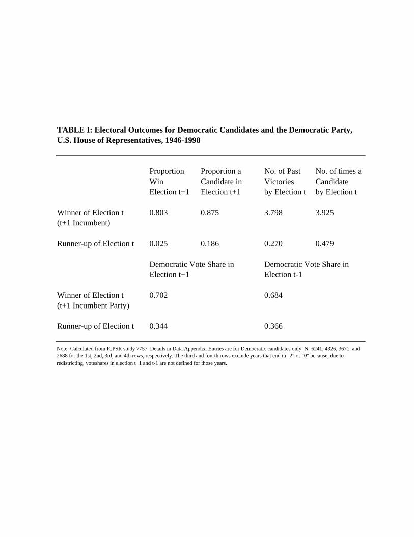
TABLE I: Electoral Outcomes for Democratic Candidates and the Democratic Party,U.S. House of Representatives, 1946-1998

Proportion Proportion a No. of Past No. of times aWin Candidate in Victories CandidateElection t+1 Election t+1 by Election t by Election t

Winner of Election t 0.803 0.875 3.798 3.925(t+1 Incumbent)

Runner-up of Election t 0.025 0.186 0.270 0.479

Democratic Vote Share in Democratic Vote Share inElection t+1 Election t-1

Winner of Election t 0.702 0.684(t+1 Incumbent Party)

Runner-up of Election t 0.344 0.366

Note: Calculated from ICPSR study 7757. Details in Data Appendix. Entries are for Democratic candidates only. N=6241, 4326, 3671, and 2688 for the 1st, 2nd, 3rd, and 4th rows, respectively. The third and fourth rows exclude years that end in "2" or "0" because, due to redistricting, voteshares in election t+1 and t-1 are not defined for those years.

Variable All |Margin|<.5 |Margin|<.05 Parametric fitWinner Loser Winner Loser Winner Loser Winner Loser

Democrat Vote Share 0.698 0.347 0.629 0.372 0.542 0.446 0.531 0.454Election t+1 (0.003) (0.003) (0.003) (0.003) (0.006) (0.006) (0.008) (0.008)

[0.179] [0.15] [0.145] [0.124] [0.116] [0.107]

Democrat Win Prob. 0.909 0.094 0.878 0.100 0.681 0.202 0.611 0.253Election t+1 (0.004) (0.005) (0.006) (0.006) (0.026) (0.023) (0.039) (0.035)

[0.276] [0.285] [0.315] [0.294] [0.458] [0.396]

Democrat Vote Share 0.681 0.368 0.607 0.391 0.501 0.474 0.477 0.481Election t-1 (0.003) (0.003) (0.003) (0.003) (0.007) (0.008) (0.009) (0.01)

[0.189] [0.153] [0.152] [0.129] [0.129] [0.133]

Democrat Win Prob. 0.889 0.109 0.842 0.118 0.501 0.365 0.419 0.416Election t-1 (0.005) (0.006) (0.007) (0.007) (0.027) (0.028) (0.038) (0.039)

[0.31] [0.306] [0.36] [0.317] [0.493] [0.475]

Democrat Political 3.812 0.261 3.550 0.304 1.658 0.986 1.219 1.183Experience (0.061) (0.025) (0.074) (0.029) (0.165) (0.124) (0.229) (0.145)

[3.766] [1.293] [3.746] [1.39] [2.969] [2.111]

Opposition Political 0.245 2.876 0.350 2.808 1.183 1.345 1.424 1.293Experience (0.018) (0.054) (0.025) (0.057) (0.118) (0.115) (0.131) (0.17)

[1.084] [2.802] [1.262] [2.775] [2.122] [1.949]

Democrat Electoral 3.945 0.464 3.727 0.527 1.949 1.275 1.485 1.470Experience (0.061) (0.028) (0.075) (0.032) (0.166) (0.131) (0.23) (0.151)

[3.787] [1.457] [3.773] [1.55] [2.986] [2.224]

Opposition Electoral 0.400 3.007 0.528 2.943 1.375 1.529 1.624 1.502Experience (0.019) (0.054) (0.027) (0.058) (0.12) (0.119) (0.132) (0.174)

[1.189] [2.838] [1.357] [2.805] [2.157] [2.022]

Observations 3818 2740 2546 2354 322 288 3818 2740

Table II: Electoral Outcomes and Pre-determined Election Characteristics: Democratic candidates,Winners vs. Losers: 1948-1996

Note: Details of data processing in Data Appendix. Estimated standard errors in parentheses. Standard deviations of variables in brackets. Data include Democratic candidates (inelection t). Democrat vote share and win probability is for the party, regardless of candidate. Political and Electoral Experience is the accumulated past election victories and electionattempts for the candidate in election t, respectively. The "opposition" party is the party with the highest vote share (other than the Democrats) in election t-1. Details of parametric fitin text.

(1) (2) (3) (4) (5) (6) (7) (8)

Dependent Variable Vote Share Vote Share Vote Share Vote Share Vote Share Res. Vote 1st dif. Vote Vote Sharet+1 t+1 t+1 t+1 t+1 Share, t+1 Share, t+1 t-1

Victory, Election t 0.077 0.078 0.077 0.077 0.078 0.081 0.079 -0.002(0.011) (0.011) (0.011) (0.011) (0.011) (0.014) (0.013) (0.011)

Dem. Vote Share, t-1 ---- 0.293 ---- ---- 0.298 ---- ---- ----(0.017) (0.017)

Dem. Win, t-1 ---- -0.017 ---- ---- -0.006 ---- -0.175 0.240(0.007) (0.007) (0.009) (0.009)

Dem. Political Experience ---- ---- -0.001 ---- 0.000 ---- -0.002 0.002(0.001) (0.003) (0.003) (0.002)

Opp. Political Experience ---- ---- 0.001 ---- 0.000 ---- -0.008 0.011(0.001) (0.004) (0.004) (0.003)

Dem. Electoral Experience ---- ---- ---- -0.001 -0.003 ---- -0.003 0.000(0.001) (0.003) (0.003) (0.002)

Opp. Electoral Experience ---- ---- ---- 0.001 0.003 ---- 0.011 -0.011(0.001) (0.004) (0.004) (0.003)

Note: Details of data processing in Data Appendix. N= 6558 in all regressions. Regressions include a 4th order polynomial in the margin of victory for the Democrats in Election t, with all terms interactedwith the Victory, Election t dummy variable. Political and Electoral Experience is defined in notes to Table II. Column (6) uses as its dependent variable the residuals from a least squares regression on theDemocrat Vote Share (t+1) on all the covariates. Column (7) uses as its dependent variable the Democrat Vote Share (t+1) minus the Democrat Vote Share (t-1). Column (8) uses as its dependent variablethe Democrat Vote Share (t-1). Estimated standard errors (in parentheses) are consistent with state-district-decade clustered sampling.

Table III: Effect of Winning an Election on Subsequent Party Electoral Success: Alternative Specifications, and Refutability Test, Regression Discontinuity Estimates

Dependent Variable (t+1) Candidate Candidate Party Vote Party Victory Candidacy Share Victory

Overall Estimate of Effect 0.450 0.434 0.078 0.385of Victory (t) (0.031) (0.032) (0.011) (0.036)

Sub-groups, by Experience (t)Experience=0 0.431 0.502 0.084 0.388

(0.043) (0.039) (0.013) (0.052)

Interaction: 0.027 -0.181 0.004 -0.1140<Experience<=2 (0.104) (0.107) (0.031) (0.15)

Interaction 0.008 -0.123 -0.116 -0.249Experience>2 (0.09) (0.115) (0.052) (0.183)

p-value 0.966 0.164 0.078 0.328F-test of Equal Coefficients

Sample Size 9674 9674 6558 6558

Table IV: Effect of Winning an Election on Candidate Electoral Success, Candidacy, and Party Vote Share and Electoral Success: Overall and by Experience (t) groups, Regression Discontinuity Estimates

Note: Details of data processing in Data Appendix. Least Squares Estimates for for Democrat candidates in Election t. Estimated standarderrors (in parentheses) are consistentwith candidate-levelclustering for the first two columns, and state-district-decadeclustered sampling, forthe second two columns. Sub-groups defined by Political Experience as of Election t. All columns include a 4th order polynomial in theDemocratic margin of victory (with interactions with sub-groups), and Political and Electoral Experience Variables (with subgroupinteractions). Second two columns additionally include Democrat Vote Share and Victory Indicator (t-1). F-test is of the null hypothesesthatboth sub-group interactions are zero.

Regression Discontinuity Estimates

Sample Overall Exp.=0 0<Exp<=2 Exp.>2Interaction Interaction

(1) (2) (3) (4)First stage Relationship 2.832 2.656 -0.364 1.101Effect of Victory on Exp. Dif. (0.311) (0.287) (0.514) (0.982)

Reduced-Form Relationship 0.208 0.222 -0.124 0.002Effect of Victory on Vote Share (0.027) (0.032) (0.067) (0.092)Index

Structural Parameter: Implicit 0.073 0.084 -0.041 -0.034Value of a Year of Experience (0.012) (0.014) (0.029) (0.025)

Alternative Estimation Approaches

Cross-sectional OLS 0.060 0.052 0.032 -0.031(0.002) (0.003) (0.012) (0.004)

"Fixed Effect" (Differencing) 0.022 0.031 0.000 -0.016Estimator (0.003) (0.005) (0.008) (0.007)

Instrumental Variable Estimate 0.103 0.151 0.018 -0.065(Victory in Election t as (0.002) (0.006) (0.014) (0.008)Instrument)

Sample Size 5186 5186 ---- ----

Table V: Structural Estimation of Implicit Voters’ Valuation of Political Experience, Overall and by Experience (t) Sub-groups: Regression Discontinuity Estimates and Alternative Estimation Approaches

Note: Details of data processing in Data Appendix.Estimates for Democrat candidates in Election t. Estimated standard errors (inparentheses) are consistent with state-district-decade clustered sampling. Sub-groups defined by Political Experience as ofElection t. All regression discontinuity estimates include a 4th order polynomial in the Democratic margin of victory (t) (andinteractions with Democratic Victory (t) indicator). Details of Alternative Specifications in text.