HAL Id: tel-01258843https://tel.archives-ouvertes.fr/tel-01258843

Submitted on 19 Jan 2016

HAL is a multi-disciplinary open accessarchive for the deposit and dissemination of sci-entific research documents, whether they are pub-lished or not. The documents may come fromteaching and research institutions in France orabroad, or from public or private research centers.

L’archive ouverte pluridisciplinaire HAL, estdestinée au dépôt et à la diffusion de documentsscientifiques de niveau recherche, publiés ou non,émanant des établissements d’enseignement et derecherche français ou étrangers, des laboratoirespublics ou privés.

The effects of wind-induced mixing on the structure andfunctioning of shallow freshwater lakes in a context of

global change.Lydie Blottiere

To cite this version:Lydie Blottiere. The effects of wind-induced mixing on the structure and functioning of shallowfreshwater lakes in a context of global change.. Biodiversity and Ecology. Université Paris Saclay(COmUE), 2015. English. �NNT : 2015SACLS016�. �tel-01258843�

NNT : 2015SACLS016

THESE DE DOCTORAT

DE L‟UNIVERSITE PARIS-SACLAY,

préparée à l‟Université Paris-Sud

ÉCOLE DOCTORALE N° 567

Sciences du Végétal : du Gène à l‟Ecosystème

Spécialité de doctorat (Biologie)

Par

Mme Lydie Blottière

The effects of wind-induced mixing on the structure and functioning of shallow

freshwater lakes in a context of global change.

Thèse présentée et soutenue à Université Paris-Saclay, le 8/10/2015 :

Composition du Jury :

Mr, Huisman, Jef

Mr, Cecchi, Philippe

Mr, Lacroix, Gérard

Mme, Quiblier, Catherine

Mme, Shykoff, Jacqui

Mme, Lecomte, Jane

Mme, Hulot, Florence

Directeur de recherches Université d‟Amsterdam

Chargé de recherches IRD Université de Montpellier

Chargé de recherches IEES Paris

Maître de conférences Université Paris Diderot

Directrice de recherches Université Paris-Saclay

Professeur, Université Paris-Saclay

Maître de conférences Université Paris-Saclay

Rapporteur

Rapporteur

Examinateur

Examinatrice

Examinatrice

Présidente

Directrice de thèse

3

Acknowledgement – Remerciements

First and foremost, I would like to thank the members of the jury for kindly accepting to review my work

and coming to the defense.

I would like to thank the University Paris-Sud, the doctoral school “Sciences du vegetal” and the

Ecologie, Systématique and Evolution laboratory for making this thesis possible.

En français maintenant,

Je tiens à remercier, du fond du cœur, ma directrice de thèse, Florence Hulot, pour l‟aventure humaine que

nous avons vécue, tout ce qu‟elle m‟a donné et appris. Merci de m‟avoir fait grandir, de m‟avoir fait

confiance et donné l‟appui et le soutien nécessaire à l‟aboutissement de ce travail. Je te suis infiniment

reconnaissante également de m‟avoir fait découvrir le Zimbabwe, ces deux précieuses semaines là-bas

resteront gravées dans ma mémoire pour toujours.

A Carmen, merci pour les 4 années de partage de bureau, de m‟avoir écoutée quand ça n‟allait pas et

quand ça allait bien aussi ! Pensées à Colbert, John Oliver et Jon Stewart.

Merci à l‟équipe écophysiologie végétale de m‟avoir accueillie comme l‟une des vôtres. Votre bonne

humeur, les discussions incroyables et l‟ambiance soudée de cette équipe ont été une resource essentielle

pendant toute la durée de mon doctorat.

A mes stagiaires, Mourad, Mégane, Margaux, Loïc et Brieuc, merci pour tous ces excellents moments sur

le terrain en votre compagnie, votre très bon travail et votre bonne humeur !

A Nina, merci de votre soutien infaillible, de m‟avoir aidée à traverser les épreuves, et d‟avoir cru en moi

du début à la fin.

A mes merveilleux amis, merci pour votre soutien, votre amitié ô combien précieuse. Ambre, merci

d‟avoir été présente et de m‟avoir soutenue pendant ces 4 années. Adélaïde, loin des yeux, près du cœur,

je suis heureuse d‟avoir vécu ma thèse en même temps que toi, de t‟avoir comme amie depuis tant

d‟années. Elena, tu as été l‟une de mes plus belles rencontres pendant cette thèse, tu es un vrai modèle à

suivre, muchas gracias por las flores, los estímulos y apoyo : « tu peux ! ». Alice, ma co-thésarde des bons

et des mauvais moments, nous avons traversé tout ce périple ensemble et tu as toujours été là pour me

soutenir et m‟encourager. Elodie, merci pour ta bonne humeur au laboratoire, il ne te reste que quelques

2

mois et c‟est fini ! Courage ! Lisa, merci de m‟avoir remise sur pied en cette fin de thèse, de m‟avoir fait

découvrir la plongée et d‟être toujours la chercheuse passionnée que j‟ai connue lors de mon premier stage

avec toi. J‟espère vraiment qu‟un jour prochain, nous pourrons travailler ensemble ! Malou, séparées par

la vie et réunies ces deux dernières années, merci de t‟être installée dans ce no man’s land qu‟est Fontaine

Michalon, pour ta bonne humeur, ton soutien, et tous ces apéros ! Pauline, amie depuis la licence, toi aussi

tu te lances dans l‟aventure de la thèse, bon courage ! Gabriel, tu es devenu un de mes plus proches amis

pendant cette thèse, merci de ta collaboration dans le travail, de m‟avoir appris des astuces sur Matlab, et

pour les innombrables soirées sushis. Joannes, je crois qu‟on aura tout vécu en 4 ans toi et moi ! Merci

pour la colloc‟, les soirées, la musique, les week-ends au labo… Elie et Brieuc, merci pour votre

enthousiasme, les jeux vidéo, Xavier Dolan, Adventure Time et pour tous ces supers moments ensembles.

Agathe, ma cravate, merci pour les années de lycée inoubliables, j‟ai tellement ri avec toi ! Merci d‟être

restée en contact malgré tes périples autour du monde. A notre prochaine rencontre que j‟attends avec la

plus grande impatience.

Une pensée particulière à Benoît, mon ami d‟enfance, qui nous a quittés beaucoup trop tôt.

Enfin, ma famille, c‟est grâce à vous si tout cela a été possible. Mes parents, vous avez toujours soutenu

mes projets, vous n‟avez eu de cesse de m‟encourager et de faire tout votre possible pour m‟offrir la

meilleure éducation. Vous m‟avez insufflé l‟amour, l‟admiration et le respect de la Nature, vous avez, en

grande partie façonné qui je suis aujourd‟hui. Merci pour votre amour et votre bienveillance à mon égard.

A mon frère, Gaël, tu as été un grand frère exceptionnel, tu m‟as appris des millions de choses comme la

persévérance et cette envie de résoudre mystères et énigmes et je suis sûre que tu ne le sais même pas ! A

ma famille, je vous dédie cette thèse en guise de remerciement pour tout ce que vous avez fait pour moi.

Merci !

3

Table of contents

4

Introduction ..................................................................................................................................... 7

1. Shallow lakes: context and definition ............................................................................................ 9

2. Structure of shallow lakes: the effect of wind-induced mixing.................................................. 12

2.1. Wind-induced mixing and resuspension events ........................................................................................... 12

2.2. The effects of wind-induced mixing and resuspension on shallow lake ecosystems ................................... 16

3. Shallow lakes under anthropogenic pressures – challenges ahead ........................................... 28

3.1. Eutrophication .............................................................................................................................................. 28

3.2. Climate change ............................................................................................................................................. 30

3.3. Interaction between anthropogenic stressors: warming and eutrophication ................................................. 32

4. Objectives of the thesis .................................................................................................................. 33

4.1 Questions and goals ................................................................................................................................ 33

4.2 Chapter 1: modelling the effect of wind on algal competition in shallow lakes ..................................... 35

4.3 Chapter 2 & 3: Testing the effects of mixing using wavemakers ........................................................... 36

4.4 Chapter 4: impact of mixing and warming on freshwater foodwebs ...................................................... 37

Chapter I ........................................................................................................................................ 39

Abstract .................................................................................................................................................. 42

Introduction ........................................................................................................................................... 43

Methods .................................................................................................................................................. 46

Parameter forcings ............................................................................................................................................... 46

The dynamical model .......................................................................................................................................... 48

The reaction part .................................................................................................................................................. 54

Numerical method ............................................................................................................................................... 55

Scenarios explored .............................................................................................................................................. 56

Results .................................................................................................................................................... 57

Phytoplankton responses to pure mixing effect ................................................................................................... 57

Storm events: sediment and phosphorus resuspension ........................................................................................ 61

The impact of warming on the phytoplankton growth ........................................................................................ 63

Discussion ............................................................................................................................................... 67

Eutrophication and wind exposure ...................................................................................................................... 67

Impacts of storm events ....................................................................................................................................... 69

Effects of warming on M. aeruginosa dominance and bloom-formation ............................................................ 72

Conclusion .............................................................................................................................................. 74

Acknowledgments .................................................................................................................................. 75

References .............................................................................................................................................. 75

Appendix A: Computation of the bottom shear stress ....................................................................... 80

Appendix B: Phosphorus parameters .................................................................................................. 82

Appendix C: Figure of the effect of initial M. aeruginosa density on simulations results............... 82

Appendix D: Figure of the percentage of light lost for all depths and dates of the figure 3. .......... 83

5

Chapter II ...................................................................................................................................... 85

Abstract .................................................................................................................................................. 88

Introduction ........................................................................................................................................... 89

Physical characteristics, wind forcing and water motions in lakes ...................................................................... 89

Experimental devices manipulating the water-column structuration ................................................................... 91

Effects of waves in deep and shallow lakes ........................................................................................................ 92

Mesocosms with wavemakers: a new ecological device ..................................................................... 95

Theoretical background ....................................................................................................................................... 95

Specifications of the mesocosm with a wavemaker ............................................................................................ 98

Technical study of a prototype ............................................................................................................................ 99

Comments and recommendations ...................................................................................................... 104

Acknowledgements .............................................................................................................................. 105

References ............................................................................................................................................ 106

Chapter III ................................................................................................................................... 111

Abstract ................................................................................................................................................ 114

Introduction ......................................................................................................................................... 115

Materials and methods ........................................................................................................................ 118

Study site and experimental design ................................................................................................................... 118

Physical measurements and water chemistry .................................................................................................... 119

Phytoplankton and zooplankton ........................................................................................................................ 120

Statistical analysis ............................................................................................................................................. 121

Results .................................................................................................................................................. 122

Initial conditions ................................................................................................................................................ 122

Water mixing effects on turbidity and water chemistry .................................................................................... 123

Water mixing effects on phytoplankton ............................................................................................................ 127

Water mixing effects on zooplankton ................................................................................................................ 129

Water mixing effects on prokaryotes and virus-like particles ........................................................................... 131

Discussion ............................................................................................................................................. 132

Mixing effects on turbidity and sediments ........................................................................................................ 132

Mixing effects on nutrient concentration ........................................................................................................... 133

Mixing effects on phytoplankton and chlorophyll a concentrations ................................................................. 134

Mixing effects on pH and primary productivity ................................................................................................ 135

Mixing effects on zooplankton dynamics .......................................................................................................... 136

Mixing effects on prokaryotes and viruses ........................................................................................................ 137

Ecosystem level ................................................................................................................................................. 137

Acknowledgements .............................................................................................................................. 139

References ............................................................................................................................................ 139

Chapter IV ................................................................................................................................... 147

Abstract ................................................................................................................................................ 150

6

Introduction ......................................................................................................................................... 151

Materials and Methods ....................................................................................................................... 154

Study site and experimental design ................................................................................................................... 154

Mixing ............................................................................................................................................................... 155

Warming ............................................................................................................................................................ 155

Physical measurements and water chemistry .................................................................................................... 156

Phytoplankton and zooplankton ........................................................................................................................ 157

Statistical analysis ............................................................................................................................................. 158

Results .................................................................................................................................................. 160

Temperatures evolution and quantification of the warming effect .................................................................... 160

Effect of warming on biotic and abiotic variables ............................................................................................. 166

Effects of mixing on abiotic and biotic variables .............................................................................................. 166

Discussion ............................................................................................................................................. 176

Use of polyethylene films as a warming tool .................................................................................................... 176

On the (non)-effects of experimental warming ................................................................................................. 177

Effects of mixing – comparison with 2012 experiment ..................................................................................... 178

Conclusion ............................................................................................................................................ 180

Aknowledgments ................................................................................................................................. 180

References ............................................................................................................................................ 181

Annexe 1 ............................................................................................................................................... 184

Conclusion and perspectives ....................................................................................................... 185

Reproducibility and major experimental results .............................................................................. 189

Temporality of wind-induced mixing episodes ................................................................................. 194

Warming – results and questions ....................................................................................................... 198

General conclusion .............................................................................................................................. 201

References .................................................................................................................................... 203

Synthèse……………...………………………………………………………………………….218

Résumé. ................................................................................................................................................ 220

Abstract ............................................................................................................................................... 220

7

Introduction

Emerald Lake in the Candian Yukon. ©Matt Shetzer

8

9

1. Shallow lakes: context and definition

Shallow lakes have been a great source of scientific interest and questioning in the past

century. The incredible biodiversity, daunting complexity and the tight historical link between

these ecosystems and human societies, all represent a highway for scientific studies of all kinds.

A simple analysis of the past century publications (using the “Publish or Perish” software,

Harzing 2007) shows the high diversity of ecological inquiries focused on shallow lakes, from

water chemistry and nutrient cycling, to modelling alternative equilibria, along with

biomanipulation and trophic cascades analysis. However, because many considered inland water

bodies to be insignificant component of the biosphere, they have often been ignored in global

estimates of ecosystem processes in large scale studies (Downing et al. 2006).

Since the first estimations by Schuiling in 1977, a great effort has been made to

characterize the global abundance and distribution of freshwater bodies on Earth. Recently,

Downing and colleagues (2006), using modern techniques, gave the staggering estimation of 304

million lakes covering approximately 4.2 million km² in area. In addition to the fact that water

bodies smaller than 1 km² largely dominate lake abundance (Schuiling 1977, Wetzel 1990), they

showed that the two smallest size categories of lakes (0.001-0.01 and 0.01-0.1 km²) cover more

area than the three largest size categories (1,000-10,000; 10,000-100,000 and >100,000 km²).

Given the previous underestimation of small shallow lakes, it is likely that ecological processes

handled by freshwater bodies, such as carbon and nitrogen cycling, might have also been

underemphasized (Downing et al. 2006).

Shallow lakes and ponds form naturally in lowland areas with modest depressions in the

landscape. The natural processes involved in the origin of shallow lakes are geological

disturbances, glacial movements, or yet altered river courses or wind deflation. Humans are also

10

responsible for the creation of millions of small shallow lakes, either unintentionally, for instance

after mining activities or willfully, for agricultural, industrial or aesthetic purposes (Wetzel 2001,

Moss 2010). These lakes and ponds are extremely important for human activities and occupy a

central place in the daily life of many people (for cleaning, drinking, bathing, fishing etc.). Lakes

surroundings are usually densely populated either by necessity or for their aesthetic qualities (or

both). This led to a strong anthropogenic pressure (pollution, eutrophication) on these ecosystems

which are undergoing rapid changes in their functioning.

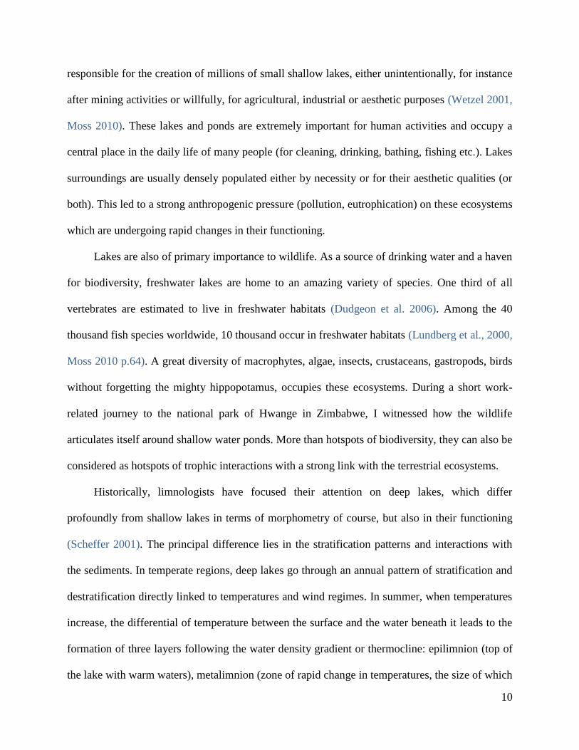
Lakes are also of primary importance to wildlife. As a source of drinking water and a haven

for biodiversity, freshwater lakes are home to an amazing variety of species. One third of all

vertebrates are estimated to live in freshwater habitats (Dudgeon et al. 2006). Among the 40

thousand fish species worldwide, 10 thousand occur in freshwater habitats (Lundberg et al., 2000,

Moss 2010 p.64). A great diversity of macrophytes, algae, insects, crustaceans, gastropods, birds

without forgetting the mighty hippopotamus, occupies these ecosystems. During a short work-

related journey to the national park of Hwange in Zimbabwe, I witnessed how the wildlife

articulates itself around shallow water ponds. More than hotspots of biodiversity, they can also be

considered as hotspots of trophic interactions with a strong link with the terrestrial ecosystems.

Historically, limnologists have focused their attention on deep lakes, which differ

profoundly from shallow lakes in terms of morphometry of course, but also in their functioning

(Scheffer 2001). The principal difference lies in the stratification patterns and interactions with

the sediments. In temperate regions, deep lakes go through an annual pattern of stratification and

destratification directly linked to temperatures and wind regimes. In summer, when temperatures

increase, the differential of temperature between the surface and the water beneath it leads to the

formation of three layers following the water density gradient or thermocline: epilimnion (top of

the lake with warm waters), metalimnion (zone of rapid change in temperatures, the size of which

11

depends on the steepness of temperature changes) and hypolimnion (layer with fairly

homogeneous cold waters in contact with the sediment bed) (Dodds & Whiles 2010 p156-161;

Reynolds 2006 p73-75). The differences in temperatures and water density between those three

layers act as a barrier for heat diffusion, wind-generated turbulences, small organisms, nutrient

exchanges or gas diffusion (Dodds & Whiles 2010 p160, Padisák and Reynolds 2003). By

contrast, stratification in shallow lakes may occur for a few hours to a few days

(microstratifications), but enhanced wind stress, reduced insolation or diel changes in

temperature will eventually rapidly overcome any structure (Scheffer 1998 p32; Reynolds 2006

p73-75, Padisák and Reynolds 2003).

In addition to the structure of the water column, deep and shallow lakes also differ greatly

in their interaction with the sediment bed. Because of the depth and stratification, the trophogenic

zone of deep lakes is largely isolated from the sediment bed (especially in summer) while in

shallow lakes, there is a quasi-constant interaction between the whole water column and the

sediments because of the lack of long-lasting stratification. This lack of segregation is of great

importance for geochemical processes (for instance, diffusion of oxygen and expulsion of carbon

dioxide and phosphorus diffusion from the sediments), vertical distribution of organisms, and

ability for macrophytes to colonize this habitat. In shallow lakes, recycling of organic matter is

also distinct from deeper lakes. In the latter, biogenic materials sink through the water column,

and while the decomposition process starts during the vertical descent, the rest of the

decomposition will take place at the bottom beyond the range of entraining shear stress (Scheffer

1998 p49). In shallow lakes, the decomposition products will rapidly regain the trophogenic zone

by diffusion or entrainment (Padisák and Reynolds 2003).

12

In all, shallow lakes can be defined as an aquatic ecosystem where at least two of the

following compartments: the littoral, the sediment bed and the entire water column, are in

constant interaction.

2. Structure of shallow lakes: the effect of wind-induced mixing

Because of their morphometry, shallow lakes are particularly vulnerable to the effects of

wind. As previously mentioned, the wind action is one of the major sources of mixing and

destratification of the water column, but it is also the main mechanism behind resuspension of the

sediments. In this section, I will discuss in more details the mechanisms and consequences of

wind-induced mixing.

2.1. Wind-induced mixing and resuspension events

As the wind blows over the surface of shallow lakes, surface waves are generated. The

physics behind wave motion is extremely complex but there are three parameters that are highly

important to understand wave

action in shallow lakes: the depth

(d), the fetch and the wind

velocity.

The fetch is the length of

the lake over which the wind

blows without interruption

(Figure 1). The longer the fetch,

the higher the waves will be for a

Figure 1. The fetch is the length of the lake (here irregularly

shaped) on which the wind of a certain direction blows. (A) The

maximal fetch of a wind blowing in the south-north direction, (B)

The maximal fetch of a wind blowing in the east-west direction.

From Dodds & Whiles 2010.

13

given wind speed. This phenomenon can be easily observed in any lake on windy days. At the

shoreline, often sheltered from the wind, the surface is quiet or slightly rippled. But further from

the shore, waves build up and become higher as the fetch extends. The maximum height (h, in

cm) of a wave on a lake appears to be proportional to the square root of the fetch (in cm) as

follows:

√

According to this equation, a lake with a fetch of 10 km will have a maximal wave height

of 1.05 m (Wetzel 2001 p.103). When the wavelength (λ) of these waves is long enough and the

lake shallow (d < λ/2), water particles underneath the surface move in an elliptical orbit. The

radius of these orbits gets smaller as they move downward in the water column and flatten near

the bottom. The horizontal oscillatory movements of the water at the bottom exert a shear stress

on the sediment bed that can generate resuspension (Figure 2).

Figure 2. Schematic representation of wave action on the water column and sediment bed in a shallow

lake. From Laenen and LeTourneau, U.S Geological survey, Portland Oregon, 1996.

14

As previously mentioned, whether resuspension occurs or not depends on the wind

velocity, water depth and fetch, but also on the sediment characteristics. Typically, the fresh

material at the top of the sediment bed requires a lower critical shear stress for resuspension than

compacted material further down in the sediments (Bengtsson & Hellström 1992). The

erodability of the sediments can be increased by bioturbation (Bakker 2012) or decreased by

algae and bacteria biofilms (Lundkvist et al. 2007). Also, fine-grained particles, for instance silt

and clay, are more easily transported than coarser particles (Luettich et al. 1990). Erosion of the

sediment bed takes place until the depth is reached where the sediment strength/cohesiveness is

equal to the erosive force (Mehta and Partheniades 1979). Therefore, the amount of resuspended

material as a function of wind speed can be represented as in figure 3.

Figure 3. Theoretical link between suspended solid concentration and wind speed for a

large/shallow lake and a smaller /deeper lake. No resuspension occurs for a certain range of wind

velocity because either the wave energy dissipates in the water column and does not reach the

sediment or the shear stress imposed at the bottom is weaker than the strength of the sediment.

When the erosive force in superior to sediment strength, resuspension increases asymptotically

until all suspendible material is in the water column. From Scheffer 1998.

15

As long as the wind blows over the lake and generates sufficient mixing, suspended

particles are moved and distributed almost evenly in the lake water (Bengtsson & Hellström

1992). In some well-exposed shallow lakes, or in very large lakes, this phenomenon can be

almost continuous. When the wind stops or at least is gentle enough, suspended particles settle at

the bottom of the lake. The length of time that particles remain suspended in the water depends

mainly on the particle settling velocity characterized by the particle size, shape and density

(Hamilton & Mitchell 1996, Zhiyao et al. 2008). Fine-grained - low density particles sediment

slowly while coarse - high density particles sediment quickly (Kristensen et al. 1992). The

complex dynamic of sediment resuspension and deposition have been extensively studied and

modelled in the 1990s‟ (Luettich et al. 1990, Van Duin et al. 1992, Bengtsson & Hellström 1992,

Blom et al. 1992, Kristensen et al. 1992, Vlag 1992, Hamilton & Mitchell 1996).

The extent to which a lake will be influenced by the wind depends also on the topography

of the lake and composition of the surroundings. Lakes surrounded by high trees blocking the

wind will have smaller fetch. Human constructions as well as deforestation might alter the wind

regimes experienced by a lake. An interesting example of this is from France 1997, who studied

the impact of riparian deforestation on the thermocline depth in the Shield Lakes in Canada. He

showed that deforestation deepened the thermocline thus compressing the hypolimnion and

increased the water lake turbidity. In shallower lakes, such variations in the fetch length could

greatly change the resuspension dynamics.

Macrophytes can also greatly influence the rate of resuspension in shallow lakes (Hamilton

& Mitchell 1997, Jeppesen et al. 1998 chapter 25). In 1959, Jackson and Starret showed that the

turbidity caused by wind-induced mixing was much higher in winter than in summer when the

vegetation covered the lake bottom. In 2007, Huang et al. observed similar patterns in Lake Taihu

in China where resuspension rates were significantly lower in zones covered by the floating-

16

leaved Trapa quadrispinosa than in zones without any macrophytes cover. Macrophytes,

especially at high density, reduce strongly the movements of the water at the sediment surface,

thus avoiding resuspension (Scheffer 1998 p48).

2.2. The effects of wind-induced mixing and resuspension on shallow lake

ecosystems

2.2.1 Underwater light climate

Cycles of resuspension and sedimentation by

wind-induced mixing affects the ecosystem in

various ways. By increasing the concentration of

suspended matter in the water column,

resuspension affects greatly the underwater light

climate. In water, the light intensity diminishes

with depth in an approximately exponential

manner:

Where z represents the depth, I the light

intensity and E the vertical attenuation coefficient

for downward irradiance (Scheffer 1998 p21).

When resuspension occurs, suspended particles

either absorb the light or scatter it in all direction

depending on their composition, size and shape

(Davies-Colley & Smith 2001). For instance, clay

Figure 4. (A) Estimated PAR as a function

of depth in condition of wind or without

wind in Lake Tämnaren (Sweden). (B)

Corresponding predicted relative algal

production (Prel). From Hellström 1991.

17

particles tend to cause scattering while dissolved organic substances absorb light (Davies-Colley

& Smith 2001). In clear waters with little or no resuspension, light easily reach the bottom of

shallow lakes, which allows for the growth of macrophytes and phytoplankton in the water

column. Light attenuation due to resuspension has two major effects on the biota: increased light

limitation for photosynthetic organisms and reduced visual range or kinetic perturbations of

animals. In a successful attempt to quantify the effect of resuspension events on algal production

in Lake Tämnaren (Sweden) Hellström (1991) showed that algal production was reduced to 15%

of its production in calm conditions (see figure 4).

In a more dramatic turn of events, the lake Apopka (128 km², mean depth 1.65m) in Florida

was struck by a hurricane in 1947 that wiped out macrophytes. Since then, a thick layer of

unstable sediment is frequently resuspended by windy episodes. This lake that was known for its

clear water became highly turbid which completely prevented the recovery of the macrophytes

bed due to the light limitation (Scheffer 1998 p5-6, Scheffer et al. 2001).

The frequency of resuspension events, which can be very high in wind-exposed large lakes,

might be one of the main factors controlling phytoplankton and macrophytes growth and

production in shallow lakes with important repercussions on the rest of the foodweb.

2.2.2 Nutrient release from the sediments

One of the most sudied effect of wind-induced resuspension is the release of phosphorus

from the sediment into the water column. Shallow lakes are very different from deep lakes in that

particular matter. In deep lakes, particlate matter rich in nutrients sink through the water column

and deposit at the bottom where they are mineralized. Nutrients will only return to the epilimnion

with seasonal turnovers when the whole lake is mixed (autumn and spring). Following this logic,

Guy et al. (1994) estimated that stratified lakes can lose up to 50% of its total phosphorus during

18

the summer. In shallow lakes, the short depth ensures rapid return of sedimented particles and

mineralized nutrients into the water column. Therefore nutrients are unlikely to be lost from the

system except when the lake is flushed, by sediment dredging or when restauration tools such as

floating macrophytes bed are used to pump the nutrients.

Nevertheless, the concentration of phosphorus of the sediments in eutrophicated lakes can

be considerable. Søndergaard et al. (2003) stated that the phosphorus pool in the sediment is often

more than 100 times higher than the pool in the lake water. Consequently, the phosphorus content

in the water will depend largely on the sediment-water interactions.

Three mechanisms are involved in phosphorus loading in shallow lakes : molecular

diffusion, turbulent diffusion and resuspension (Thomas & Schallenberg 2008). The shear stress

exerted at the top of the sediment by wind-induced mixing will determine which process will take

place (see figure 5).

Figure 5. The three mecanisms of internal nutrient-loading in relation to wind-speed. In calm

conditions, with benthic shear stress τ < 𝝈𝟏, molecular diffusion is the only loading process. When wind

induces a shear stress at the bottom comprised between 𝝈𝟏 <τ < 𝝈𝟐, pore-water nutrients are

transported in eddies to the water column (turbulent diffusion). Finally, when the wind-induced mixing

is high enough the erode the surface sediments (τ > 𝝈𝟐), the main mecanism of nutrient loading is

through resuspension.From Thomas & Schallenberg 2008.

19

Molecular diffusion is a passive mecanism related to calm conditions that occur when there

is a gradient of nutrient concentration between the sediments and the water column. The diffusion

rate depends highly on physical and chemical properties of the water. The classic explanation of

phosphorus diffusion is the Redox conditions in the surface sediment : Einsele (1936) and

Mortimer (1941) described how iron (III) and phosphorus bind and precipitate under oxic

conditions, whereas in anoxic conditions iron (III) is reduced to iron (II) and both phosphorus and

iron are brought back in solution. In shallow lakes, we could stipulate that the water column is

well oxygenated especially under mixing conditions. Soluble phosphorus coming from the anoxic

sediment are therefore trapped in a narrow oxic layer at the bottom surface. When this layer

becomes anoxic, for exemple when temperatures increase and oxygen is consumed by the

organisms, this microlayer can break and release the retained phosphorus. In addition when this

microlayer is saturated, phosphorus may simply pass through and reach the water column. High

pH (which reduces iron-phosphorus binding, Lijklema 1976), increase in temperatures (Jeppesen

et al. 1997) and benthic bioturbation, are, among other factors, also implicated in phosphorus

diffusion (reviewed in Søndergaard et al. (2003)).

Turbulent diffusion happens when the shear stress due to wind action is enough to transport

pore-water nutrients (nutrients contained in intersticial water of the surface sediments) in eddies.

The fluxes of nutrient resulting from this mecanism are deemed several orders of magnitude

greater than molecular diffusion (Portielje & Lijklema 1999, Haugan & Alendal 2005).

Resuspension of the sediments can rapidly change the concentration of phosphorus in the

water (exemple Figure 6; Hamilton & Mitchell, 1997, Ogilvie & Mitchell 1998, Zhu et al. 2005).

By simulating resuspension events on sediments sampled in Lake Arresø, Søndergaard et al.

(1992) deduced that a typical resuspension event in the lake would lead to the release of

20

150 mg of SRP m-2

(SRP : soluble reactive phosphorus, used as the best estimate of the fraction

directly available for algae). This number indicates that the internal loading induced by

resuspension is 20-30 times more important than the release from undisturbed sediments in this

lake. In other shallow lakes, inter-annual variation in internal phosphorus loading was shown to

be controlled mostly by wind mixing (Jones and Welch, 1990). Thomas & Schallenberg (2008)

also calculated that wind induced resuspension was the main mecanism involved in internal

nutrient loading.

However, it is important to note that while resuspension increases the concentration of

suspended solids, concomitant increase in phosphorus concentration is not always observed. The

release of phosphorus depends also on equilibrium conditions between the sediments and the

water column. Søndergaard et al. (1992) showed that a second resuspension simulation conducted

the day after the first one did not lead to any further release of soluble reactive phosphorus. In

short, if there is an equilibrium between the phosphorus bound to suspended particles and the

water content of phosphorus, then no release will be observed. As mentioned earlier,

macrophytes can greatly reduce resuspension events, and consequently decrease the internal

phosphorous loading in shallow lakes. For instance, dense macrophyte beds of submerged and

Figure 6. Example of a lake water changes in suspended solids concentrations (left) and the concomitant

total phosphorus concentration (right) during 10 days of varying wind speed (0-2 to 5-7 to 2-3 m.s-1

). Lake

Vest Stadil Fjord, 450 ha and mean depth 0.8 m, Denmark. Reproduced from Søndergaard et al. (1992).

21

emergent plants have been shown to reduce internal loading on average by 12 and 26 mg m-2

d-1

respectively in the shallow Kirkkoja¨basin in Iceland (Horppila & Nurminen 2005).

2.2.3 Direct effects of mixing on phytoplankton: horizontal and vertical entrainment

Water movements generated by wind are essential to understand the horizontal and

vertical distribution of phytoplankton in the water column. Far from being homogeneous, the

phytoplankton distribution can be highly variable in both vertical and horizontal planes

(Reynolds 2006 p.84). However, horizontal and vertical distributions do not depend on the same

mechanisms and do not take place at the same time-scale.

In well-exposed lakes, wind forcing generates internal currents that transport

phytoplankton cells. Using a complex model of hydrodynamic transport for a lake of medium

depth (10km of fetch, 10m depth), Verhagen (1994) concluded that the horizontal distribution of

phytoplankton in response to changes of wind speed can take weeks while the vertical response is

usually within 24h. In the large shallow lake Taihu in China, the horizontal distribution of the

buoyant, bloom-forming cyanobacteria Microcystis aeruginosa was shown to depend mainly on

Figure 7. Pictures taken at the Lake Viaud (Saint-Viaud, France). On the left picture, we can observe

the high density of phytoplankton (M. aeruginosa) at the shoreline. A white dotted line is traced to show

the color difference between the shore and the open lake area. On the right picture, close-up on the lake

shore, where M. aeruginosa colonies accumulate due to wind-drift. Pictures from L. Blottière.

22

surface wind drift and to a lesser extent to internal currents (Wu et al. 2010). Wind drift is

especially relevant for buoyant phytoplankton species that colonize the surface of the water (see

figure 7).

The vertical distribution of the phytoplankton depends mainly on two parameters: their

buoyancy and the degree of mixing. In calm conditions, most of non-motile phytoplankton

species sink through the water column following Stokes equation:

Where vs (m s-1

) is the sinking velocity, g (m s-2

) is the gravitational acceleration, r (m) is

the radius of the sinking spherical particle, ρ’ and ρ are the volumic mass (or density) of the

particle and the volumic mass of the liquid medium (kg m-3

), respectively. (kg m-1

s-1

) is the

medium viscosity and is the form resistance factor (dimension-less) that captures the resistance

to sinking due to the shape of the particle relatively to a sphere ( ) (Padisák et al.

2003). Sinking is a major constraint for phytoplankton cells. In order to maintain the population,

at least a fraction of the cells must stay long enough in the photic zone to accumulate enough

carbon via photosynthesis for the next cellular replication (Reynolds 2006 p38).

In the equation above, only three variables, the size r, the density ρ’ and the form resistance

, are properties of the organism and therefore open to adaptation and/or evolution. The smaller

the particle, the slower it will sink through the water column. However, a trade-off seems to exist

between being small and thus being easily predated by zooplankton grazers (Padisák et al. 2003,

Litchman & Klausmeier 2008), and being large and sinking more rapidly. It is also hypothesized

that by sinking through the water column, larger algae increase their chance of contact with

nutrients by disrupting nutrient gradients around the cell (Wetzel 2010 p345).

23

The cytoplasm of living cells is composed mainly of water but also contains proteins,

carbohydrates, nucleic acids, and in the case of diatoms : exoskeletal structures in silica which

make the cells more dense than water. This excessive density can be overcome by multiple

mecanisms: oil droplets or lipids accumulation in the cytoplams (for instance, the green algae

Botryococcus sp. can contain lipids up to 30-40% of dry weight which enables them to float

(Fogg 1965), gas vacuols in cyanobacteria (such as M. aeruginosa seen earlier that can colonize

the surface of calm, unexposed waters), or ion regulation (which occurs mainly in species living

in salty or brackish waters and consists in replacing the heavy elements Na+ and SO4

2- by the

lighter element K+ and Cl

-).

Finally, the third variable that modulates cells sinking rate is the resistance form. In a truly

original and pedagogic experiment, Padisák et al. (2003) reproduced phytoplankton cells of

various shapes and sizes in PVC and measured the sinking velocity through a glycerine medium

(the materials were specifically chosen to respect the density difference between algae and

water). They demonstrated that a large variety of forms found in natural phytoplankton (rod-like,

coiled filaments, flat coenobs, etc) have and therefore contribute to the reduction of cell

sinking velocity.

These differences in sinking velocities are crucial for understanding the competition

between different species. Species that can regulate their position in the water column such as

swimming or buoyant species have a clear advantage in calm conditions or in wind-sheltered part

of lakes compared to heavy, sinking species that rely on mixing to reach the euphotic zone. A

great exemple of that is the bloom-forming cyanobacterium M. aeruginosa. This ubiquitous

colonial species is well-known for its massive surface scums (centimeters thick) in eutrophicated

lakes in late summer (Figure 7) (Reynolds & Walsby 1975, Paerl et al. 2001, Chen et al. 2003, de

Figueiredo et al. 2004, Jöhnk et al. 2008, Wu et al. 2010). Buoyancy regulation in this species is

24

achieved through changes in gas vacuole:cell-volume ratio and responds to various

environmental variables such as light (Reynolds 1973, Thomas & Walsby 1985, Reynolds et al.

1987, Kromkamp & Mur 1984, Wallace & Hamilton 1999), temperatures (Thomas & Walsby

1986, Kromkamp et al. 1988) and nutrients availability (Brookes & Ganf 2001). Under weak

mixing conditions, this cyanobacterium enhances its access to light while shading other non-

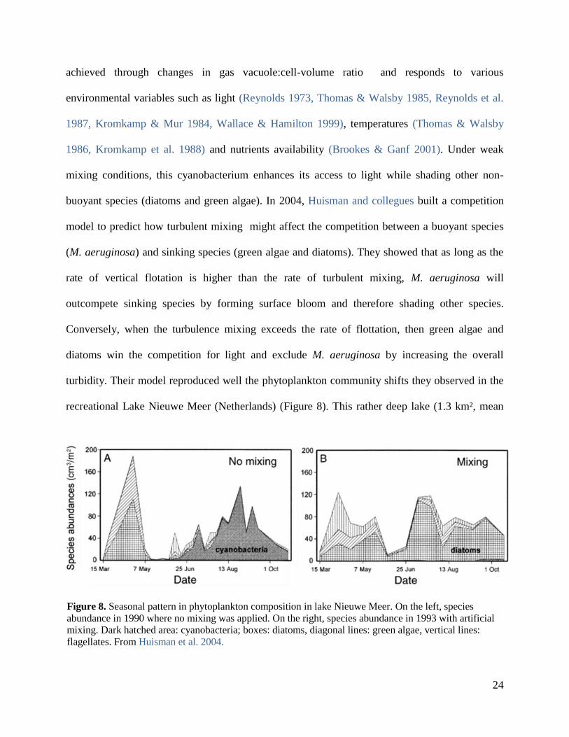
buoyant species (diatoms and green algae). In 2004, Huisman and collegues built a competition

model to predict how turbulent mixing might affect the competition between a buoyant species

(M. aeruginosa) and sinking species (green algae and diatoms). They showed that as long as the

rate of vertical flotation is higher than the rate of turbulent mixing, M. aeruginosa will

outcompete sinking species by forming surface bloom and therefore shading other species.

Conversely, when the turbulence mixing exceeds the rate of flottation, then green algae and

diatoms win the competition for light and exclude M. aeruginosa by increasing the overall

turbidity. Their model reproduced well the phytoplankton community shifts they observed in the

recreational Lake Nieuwe Meer (Netherlands) (Figure 8). This rather deep lake (1.3 km², mean

Figure 8. Seasonal pattern in phytoplankton composition in lake Nieuwe Meer. On the left, species

abundance in 1990 where no mixing was applied. On the right, species abundance in 1993 with artificial

mixing. Dark hatched area: cyanobacteria; boxes: diatoms, diagonal lines: green algae, vertical lines:

flagellates. From Huisman et al. 2004.

25

depth: 18m) experiences dense blooms of M. aeruginosa during summer months. In order to

solve this problem, bubbling systems have been installed above the sediment. This artificial

mixing led to a dramatic change in community composition from almost monospecific population

of M. aeruginosa to a mixture of green algae, diatoms and flagellates (Visser et al. 1996, Jungo

et al. 2001).

This idea that the level of mixing (natural or artificial) led to shifts in community

composition is not new. In the 1970s and 1980s, it became increasingly recognized that changes

in mixing regimes, particularly changes in stratification-destratifications in deep lakes in autumn

and spring, was responsible in part for the annual succession of phytoplankton groups (Round

1971, Reynolds 1980a, b, 1982, Reynolds et al. 1983, 1984, Sommer et al. 1986, 2012), diatoms

being favored by intense mixing and buoyant species being favored by summer stratification.

While artificial mixing was already used in many reservoirs in order to avoid anoxic hypolimnion

and its consequences (Dunst et al. 1974); in 1984, Reynolds proposed to use intermittent artificial

mixing to control phytoplankton biomass, especially in eutrophic storages suffering from

cyanobacterial blooms.

Since then, artificial mixing using bubbling systems, has been widely used to control

cyanobacterial blooms in eutrophic and hypereutrophic lakes. However, due to high energy

consumption and cost, this method is not applicable in small lakes. Another drawback is that the

influence of bubbling systems is limited to the plume of each air diffuser. Recently, another

system called Solar Powered Circulation (SPC) has been tested on lakes of different sizes and

depths (Hudnell et al. 2010). It proved very efficient except in very shallow lakes (less than 1m

deep) where the system could not control the populations of cyanobacteria.

26

Figure 9. Regression of surface chlorophyll a in Lake

Apopka (Florida) on average daily wind speed.

Redrawn from Schelske et al. 1995.

In shallow lakes, water mixing has a more complex outcome than in deep lakes. Whether

the source of the mixing is artificial or wind-induced, the mixing extends usually to the whole

water column. While it may increase water turbidity and therefore hinder algae growth and

productivity, it may also resuspend nutrients, and bring back sedimented algae to the euphotic

zone. In the absence of wind, sinking algae settle on top of the sediments. Many phytoplankton

species are able to survive temporally in cellular resting stages that are induced by darkness. This

benthic population of dormant algae (mainly composed of planktonic diatoms, vegetative

colonies or asexual spores of cyanobacteria and cysts of dinoflagellates) is called the

meroplankton and can be 5-10 cm thick with chlorophyll a concentrations up to 10-fold that of

the surface waters (Reynolds 2006, Schelske et al. 1995). During wind-induced mixing, the

meroplankton is brought back in the water column where it is exposed to light. Within a few

hours of exposition, resting cells become physiologically active. Carrick et al. (1993) found that

the resuspension of meroplankton could

double the algal biomass in the surface

water in Lake Apopka (Florida, surface

area: 124.6 km², mean depth: 1.7m).

In a following paper on

meroplankton resuspension, Schelske and

collegues (1995) demonstrated that

chlorophyll concentrations above 100 µg

L-1

in Lake Apopka were highly

correlated with wind speed, the latter

explaining 53% of the temporal

27

variability in chlorophyll content (Figure 9).

Similarly, in 2004 and 2005 Verspagen and colleagues carried out field measurements in

lake Volkerak (The Netherlands) in order to assess the importance of benthic recruitment of

overwintering populations of M. aeruginosa. They discovered that without benthic recruitment,

summer blooms would be reduced by 50%. In addition, it was shown that the most viable

colonies were surviving in the shallow parts of the lake where resuspension events from wind

action could easily inoculate M. aeruginosa propagules in the water column and lead to bloom

formation.

2.2.3 Indirect effects of mixing on phytoplankton

In light of the foregoing, it is clear that wind-induced mixing affects the whole ecosystem

of shallow lakes via different pathways: sediment resuspension, nutrient release and also via

direct effect on phytoplankton recruitment and competition. Increased light-limitation due to

sediment resuspension can hinder phytoplankton growth and can cause a drop in production as

shown by Hellström (1991). At the same time, nutrient release, and especially phosphorus can act

as a boost of phytoplanktonic growth when previous nutrient-limitation exists. And finally, the

loss of phytoplankton due to high turbidity can be compensated or even overcome by benthic

recruitment.

A few studies attempted to understand the relative importance of each process. In their

study on meroplankton recruitment, Carrick et al. (1993), despite some uncertainties, considered

that the release of nutrients following resuspension was not enough to explain the observed

increase in chlorophyll a. In a controlled experiment, Schallenberg & Burns (2004) showed that

entrainment of meroplankton was the most important effect following resuspension. The level of

turbidity was not enough to induce light-limitation, and the nutrient release proved to be small

28

compared to the usual nutrient content of the water. Moreover, they showed that particulate total

phosphorus and total nitrogen increased, but not dissolved nutrient concentration, which is the

only form directly available for algae. Conversely, Ogilvie and Mitchell (1998) observed a

positive effect of nutrient release on algal biomass and production and a positive effect of

turbidity via a reduction of light-inhibition.

Clearly, the outcome of mixing is complex and depends on the duration and frequency of

mixing events and on the previous state of the lake and the time scale considered. On the short

term, resuspension induced by storms may deeply change the underwater light climate and the

nutrient content. On larger time scale, regular wind-induced mixing plays a role on species

selection and might be determinant for the trophic foodweb structure, nutrient cycles and overall

productivity of the lake.

3. Shallow lakes under anthropogenic pressures – challenges ahead

3.1. Eutrophication

Shallow lakes, alongside all ecosystems, are facing multiple anthropogenic pressures,

especially since the industrial revolution (Strayer & Dudgeon 2010). Among others, nutrient

pollution, that is, man-made eutrophication can profoundly alter aquatic ecosystem structure and

functioning. Compared to natural eutrophication, “cultural eutrophication” occurs rapidly,

especially in densely populated area (Dodds and Whiles, 2010). Agricultural fertilizers, livestock

practices, watershed disturbance and the release of nutrient-rich sewage into rivers and lakes are

the main sources of phosphorus and nitrogen enrichment. Increased algal biomass and bloom

frequency, loss of biodiversity and reduced water quality are typical consequences of nutrient

loading (see Fig. 10).

29

Figure 10. Some biological and economical effects of excessive nutrient loading on freshwater ecosystems.

Up arrows : increase, down arrows : decrease, double arrows : increase or decrease depending on the

amount of nutrient added to the system. . Reproduced from Dodds et al. 2009.

Shallow lakes are particularly vulnerable to eutrophication because of their high

surface/volume ratio and their intense water-sediment interactions. In order to limit the costly

consequences of eutrophication, many restoration plans involving dramatic cuts in nutrient inputs

have been put in place in the past 60 years such as the EU Water Framework Directive

(Søndergaard et al. 2001). While some lakes respond rather rapidly to the reduced phosphorus

loading, other lakes responses are very slow (Marsden 1989, Jeppesen et al. 1991, van der Molen

et al. 1994, Phillips et al. 2005). The reason behind this delay is the substantial quantities of

phosphorus that accumulates in the sediments during periods of high external loading

(Søndergaard et al. 2001, 2003). As seen in the previous sections (2.2.1), internal loading through

30

molecular diffusion, turbulent diffusion or resuspension maintain high phosphorus concentrations

in the water column.

3.2. Climate change

In the last decades, climate change has been recognized as one of the major threat on

biodiversity at global, regional and local scales (Heino et al. 2009). Since the 1950s, many

changes due to climate warming have been observed and most of them are unprecedented over

decades to millennia. Over the period 1880 to 2012, the combined land and ocean surface

temperatures have increased by 0.85 [0.65 to 1.06]°C and are projected to keep on rising over the

21st century. In order to anticipate the effect of global change on temperatures, integrated

assessment models have been used to produce four Representative Concentration Pathways

(RCPs) based on greenhouse gases emission scenarios for the century (IPCC report, 2014).

According to those scenarios, global average temperatures will increase by 1.0 [0.3 to 1.7]°C in

the best case scenario and by 3.7 [2.6 to 4.8] in the worst case scenario by 2100 (Table 1).

Table 1. Projected change in global mean surface temperature for the mid- and late 21st century

relative to the 1986-2005 period. From the IPCC climate change 2014 synthesis report p.60.

2046-2065 2081-2100

Scenario Mean Likely range Mean Likely range

Global mean

surface

temperature

change (°C)

RCP2.6 1.0 0.4 to 1.6 1.0 0.3 to 1.7

RCP4.5 1.4 0.9 to 2.0 1.8 1.1 to 2.6

RCP6.0 1.3 0.8 to 1.8 2.2 1.4 to 3.1

RCP8.5 2.0 1.4 to 2.6 3.7 2.6 to 4.8

31

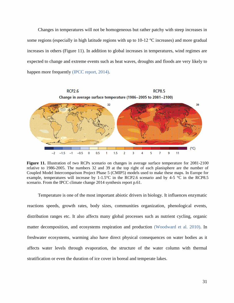
Changes in temperatures will not be homogeneous but rather patchy with steep increases in

some regions (especially in high latitude regions with up to 10-12 °C increases) and more gradual

increases in others (Figure 11). In addition to global increases in temperatures, wind regimes are

expected to change and extreme events such as heat waves, droughts and floods are very likely to

happen more frequently (IPCC report, 2014).

Temperature is one of the most important abiotic drivers in biology. It influences enzymatic

reactions speeds, growth rates, body sizes, communities organization, phenological events,

distribution ranges etc. It also affects many global processes such as nutrient cycling, organic

matter decomposition, and ecosystems respiration and production (Woodward et al. 2010). In

freshwater ecosystems, warming also have direct physical consequences on water bodies as it

affects water levels through evaporation, the structure of the water column with thermal

stratification or even the duration of ice cover in boreal and temperate lakes.

Figure 11. Illustration of two RCPs scenario on changes in average surface temperature for 2081-2100

relative to 1986-2005. The numbers 32 and 39 at the top right of each planisphere are the number of

Coupled Model Intercomparison Project Phase 5 (CMIP5) models used to make these maps. In Europe for

example, temperatures will increase by 1-1.5°C in the RCP2.6 scenario and by 4-5 °C in the RCP8.5

scenario. From the IPCC climate change 2014 synthesis report p.61.

32

Because of the urgency of the situation, many scientific studies have been published on the

effect of changes in temperatures on freshwater ecosystems. One of the well-known

consequences of rising temperatures and heat-waves is the increase in frequency and magnitude

of cyanobacterial blooms (Paerl & Huisman 2008, Jöhnk et al. 2008, Kosten et al. 2011) which

threatens water quality and ecosystem functioning. Losses in biodiversity are also predicted

because of the insular nature of freshwater habitats (Strayer & Dudgeon 2010) which limits the

ability of freshwater species to migrate across the landscape. Also, large-scale changes in

ecosystem functioning have also been demonstrated in mesocosm experiments: for instance,

increase in temperatures led to a faster rate of respiration relative to primary production causing a

reduction of carbon sequestration by 13% (Yvon-Durocher et al. 2010).

Shallow lakes might be particularly vulnerable to climate change: because of the short

depth, the thermal stress is expected to be greater than in deep lakes. Cold-water species will not

be able to migrate in colder waters during heat-waves. Furthermore, these ecosystems are

particularly at risk during droughts with longer periods of low water levels (Heino et al. 2009).

3.3. Interaction between anthropogenic stressors: warming and eutrophication

Another layer of complexity is emerging as it is becoming clear that warming and other

anthropogenic pressures have synergistic effects on freshwater ecosystems (Moss et al. 2011).

For instance, high temperatures have a positive effect on phosphorus release from the sediments

through direct effect, anoxia-mediated effect and increased mineralization rates (Jensen &

Andersen 1992, Søndergaard et al. 2003, McKee et al. 2003, Feuchtmayr et al. 2009). This

phenomenon could exacerbate the effects of eutrophication that we have seen in section 3.1

(figure 10). Rising temperatures also favors floating vegetation and blooms of cyanobacteria,

33

which are a symptom of eutrophication, through higher growth rates and water stratifications

(Paerl & Huisman 2008, Kosten et al. 2011).

Most of the water bodies in the world are suffering from cultural eutrophication and

increases in temperatures seem more and more ineluctable (at least 2°C by the end of the 21st

century). Therefore, in order to fully comprehend how freshwater shallow lakes function, it is

necessary to take into account these anthropogenic pressures in experimental and modelling

studies.

4. Objectives of the thesis

4.1 Questions and goals

The aim of this thesis is to gain a more comprehensive understanding of the influence of

mixing on shallow lake ecosystems and how the processes involved articulate themselves in a

context of anthropogenic pressures, here, eutrophication and global warming.

My work can be divided into three parts. First, I worked on a coupled hydrodynamic and

competition model inspired from the work of Huisman and colleagues and adapted it to a shallow

ecosystem. This model gave me the possibility to test multiple case-scenarios of wind-induced

mixing, from short term storms (with resuspension and nutrient release) to long term effects of

different wind-exposures on phytoplankton (a typical green algae versus M. aeruginosa)

competitions (chapter I).

In a second part, I wanted to explore the effects of mixing on the whole pelagic ecosystem.

As one can notice from the sections 2.2.1-2.2.2, the vast majority of studies on mixing focuses on

phytoplankton. Only a few studies took into account the effects of mixing on other groups such as

zooplankton (zooplankton succession: Eckert & Walz 1998, trophic-transfer: Weithoff et al.

2000, turbidity interference on zooplankton feeding rate: Levine et al. 2005), bacteria and

34

prostists (Garstecki and Wickham 2001). To my knowledge, Weithoff‟s (2000) study on the

effect of consecutive resuspension events is the only one to address the mixing effect on three

trophic levels (bacteria, phytoplankton and rotifers). Considering the importance of wind-induced

mixing on the local environment (turbidity, nutrient availability) and on phytoplankton growth

and biomass, direct and indirect impacts on higher and lower trophic levels could be expected. To

test this hypothesis, I carried out an experiment using mesocosms equipped with wave-makers.

These new systems have been adapted from fluid mechanics to ecology by Florence Hulot (ESE,

University Paris Sud, France) and Maurice Rossi (IJLRA, Paris, France). The amplitude,

frequency and length of the waves are adjustable (details in chapter II). Using this, we

successfully created two distinct environments: a water column fully mixed with resuspension of

the top sediment bed, and a water column with only superficial mixing and no resuspension. In

our experiments (2012 and 2013), we chose to work on pelagic communities without

macrophytes. This restricts our conclusions to algae-dominated shallow lakes, which is typical of

eutrophicated systems.

During the summer 2012, we followed the dynamic and composition of pelagic

communities as well as standard chemical and physical variables during 9 weeks and compared

the results between mixed and calm enclosures (chapter III). In 2013, I we applied the same

mixing treatments but this time crossed with a warming experiment using polyethylen sheets

causing a local-greenhouse effect. We followed the same variables as in 2012 and also analyzed

the warming capacity of our heating system. This set-up allowed us to assess whether shallow

ecosystems with different levels of mixing respond in a similar or different way to an increase in

water temperatures (chapter IV).

35

4.2 Chapter 1: modelling the effect of wind on algal competition in shallow lakes

The goal of the study was to model the effect of wind speed on shallow lakes using a

hydrodynamic model coupled to a phytoplankton species model. Here, the model was built to

encompass three major effects of wind-induced mixing on shallow lakes: (i) sediment

resuspension above a certain threshold of wind-induced mixing which changes the underwater

light climate, (ii) nutrient release from those sediments, (iii) vertical distribution and competition

between two phytoplankton species: a typical sinking green algae (chlorella type) and a buoyant

cyanobacteria M. aeruginosa. I studied different scenarios from short storm events to long-term

effects of different level of regular mixing. In this work, I included a gradient of phosphorus

concentration, from oligotrophic to hypereutrophic lakes, and also simulated a + 2°C warming to

understand how lakes with differing mixing regimes will respond to anthropogenic pressures.

The key results are:

Without warming, blooms of cyanobacteria are restricted to hypertrophic waters with low

wind exposure. Wind speed above 2 m.s-1

hinders bloom formation and favors the

establishment of green algae, even in hypereutrophic conditions.

With a 2°C warming, blooms of cyanobacteria are no longer confined to hypereutrophic

waters, and start to form in mesotrophic waters. Green algae are excluded in low-wind and

eutrophic conditions. They only win the competition in oligotrophic waters. Wind-induced

mixing above 3m.s-1

impairs dense bloom formation at the surface; however, there is still a

coexistence of green and cyanobacteria in the water column. If the wind stops, dense surface

scums will form immediately.

Storm events lead to a decrease in phytoplankton density because of turbidity but this effect is

rapidly compensated by the release of phosphorus.

36

The results of this modeling study were published in Theoretical Ecology in 2014.

4.3 Chapter 2 & 3: Testing the effects of mixing using wavemakers

Chapter 2 is a methodological paper describing the mesocosms used in the 2012 and 2013

experiments. A review of the effects of wind forcings and water motions is provided and other

tools used in resuspension-mixing experiments are discussed. Theoretical description and in situ

testing of the physical effect of wave makers on water motion are presented. This paper is in

preparation for submission to Limnology & Oceanography: Methods.

Chapter 3 reports the study of the impact of mixing on freshwater pelagic communities. A

9-weeks long experiment was carried out in summer 2012 using 6 mesocosms equipped with

wave-makers. Two mixing regimes were compared: “mixed” with a fully mixed water column

and resuspension of the top sediment bed and “calm” with only superficial mixing and no

resuspension. Standard chemical and physical variables were followed weekly alongside the

dynamic of phytoplankton, zooplankton, bacteria and viruses.

The key results are:

Mixing successfully induced resuspension on the sediment leading to a more turbid

environment.

Higher concentrations of chlorophyll a were found in mixed enclosures. However, we did not

find any increase in phytoplankton abundance suggesting a physiological adaption to mixing.

Photosynthetic activity was higher in mixed enclosures. This result could be explained by a

positive response of phytoplankton to fluctuating light.

Zooplankton responses varied among groups with neutral effect of rotifers and bosminas and

a negative effect of mixing on copepods.

37

Lysis of bacteria by viruses seemed enhanced in mixed enclosures probably because of an

increased contact rate.

Accumulation of nitrites, which was found in all mesocosms probably due to a dysfunction in

the nitrogen cycle, was slightly alleviated by mixing.

This study is submitted to Limnology & Oceanography.

4.4 Chapter 4: impact of mixing and warming on freshwater foodwebs

In this chapter, I describe a study on the response of freshwater pelagic communities to the

combined effects of mixing and warming. The experiment took place in the summer 2013. This

year, 12 mesocosms were used. On half of them, polyethylen sheets were installed in order to

generate a local greenhouse effect. Two mixing regimes (“Mixed” and “Calm”) were applied and

crossed with the warming treatment. As in 2012, we followed for 9 weeks physical and chemical

parameters as well as the dynamics of phytoplankton and zooplankton.

The key results:

Using polyethylen sheets, we achieved in a few days a warming effect of ~1°C throughout the

water column.

No effect of warming was found on any of the variables followed during this experiment.

However, due to technical difficulties, the warming took place only halfway through the

experiment. This reduced greatly the statistical power of the analysis and calls for caution in

the conclusions.

The mixing effect was extremely similar to the one found in 2012 with similar effects on

phytoplankton and zooplankton which suggest a robust and reproducible effect of mixing on

pelagic communities.

38

Further analyses are currently carried out in order to test the effects of mixing and warming

on bacteria, virus and also size of phytoplankton and zooplankton.

39

Chapter I

40

41

Colonies of M. aeruginosa floating at the surface of the Lake Viaud in the summer 2013 (France).

Picture from: L. Blottière

Modeling the role of wind and warming on Microcystis aeruginosa

blooms in shallow lakes with different trophic status

L. Blottière & M Rossi & F. Madricardo & F. D. Hulot

Received: 22 January 2013 / Accepted: 18 June 2013 in

Theoretical Ecology February 2014 Vol. 7 No. 1 pp. 35-52

Keywords: Microcystis aeruginosa; phosphorus resuspension; vertical mixing; wind; eutrophication; temperature

42

Abstract

This study focuses on the role of wind exposure, in interaction with trophic status and

temperature, on the competition between two species: M. aeruginosa and a typical green alga. It

is based on a water column model containing ecological and fluid mechanic features including

mixing and shear stress at the bottom. This model addresses for the first time the impact of storm

events (inducing sediment and nutrient resuspension) on algal dynamics. Simulations with

realistic environmental forcings were performed with different sets of wind, temperatures and

trophic conditions. With normal temperatures, conditions for dominance and bloom formation of

M. aeruginosa in summer are restricted to hypertrophic waters with low wind exposure. Higher

wind velocity (above 2m.s-1

) impairs the formation blooms even in phosphorus-reach waters and

enhances the dominance of green algae. Warming increases the capacity of M. aeruginosa to

develop at lower phosphorus concentrations and higher wind exposure. In hypereutrophic waters

without wind, green algae are completely excluded. Nevertheless, high wind exposure (above

3m.s-1

) still prevents dense bloom formation and allows for the coexistence of both species.

Storm events bring two counter-balancing features: sediment and nutrient resuspension. Higher

turbidity leads to a decrease of phytoplankton density due to light-limitation, while the

phosphorus release leads to an increase and better maintenance of M. aeruginosa blooms. This

result depends on the timing of the event and on general wind exposure as phosphorus release

only benefits to M. aeruginosa if exposure to wind is low.

43

Introduction

The past decades have seen an important increase of frequency and magnitude of

cyanobacterial blooms in freshwater bodies throughout the world (Graham and Wilcox 2000;

Hudnell et al. 2010a; Kosten et al. 2012). Microcystis aeruginosa, a cosmopolitan genus, often

dominates the phytoplankton community in eutrophic lakes (Reynolds 2006; Baldia et al. 2007)

and is known for its dense surface scums. Some strains produce toxins, such as microcystins,

which are released into the water during the senescence of the bloom (Jacoby et al. 2000). These

scums and toxins compromise drinking water production, recreational activities and above a

certain threshold, may have negative effects on human health (Codd et al. 1999; Carmichael et al.

2001; Zegura et al. 2003; de Figueiredo et al. 2004; Falconer and Humpage 2005; Wiegand and

Pflugmacher 2005; Hudnell et al. 2010a).

Understanding the seasonal dynamics and bloom magnitude of cyanobacteria in response

to environmental conditions thus becomes a priority if prediction and eventual prevention of

blooms are to be achieved. A variety of limnological, meteorological, chemical or biological

processes are known to promote the growth of M. aeruginosa (Soranno 1997; Jacoby et al. 2000;

Bonnet and Poulin 2002; Moss et al. 2003; Jöhnk et al. 2008; Kosten et al. 2012). First,

increasing occurrences of cyanobacterial blooms are usually symptomatic of accelerating

eutrophication, in particular of phosphorus enrichment (beyond 30 µg.L-1

) in aquatic systems

(Jacoby et al. 2000; Downing et al. 2001). Second, field observations and laboratory experiments

also indicate a strong preference of M. aeruginosa for warm temperatures with blooms occurring

predominantly during summer and beginning of autumn (Baldia et al. 2007; Havens 2008; Jöhnk

et al. 2008). In addition to these two elements (lake trophic status, water temperature), a third

factor seems particularly crucial: mixing due to wind or thermal effects. For instance, previous

44

field studies indicated that eutrophic waters, warm temperatures and little vertical mixing provide

ideal conditions for surface blooms of M. aeruginosa (Jacoby et al. 2000; Chen et al. 2003; Jöhnk

et al. 2008). This probably originates from the capacity of M. aeruginosa to regulate its buoyancy

thanks to gas vesicles allowing it to gain better vertical positions in the light gradient and migrate

to the water surface (Paerl 1988; Verspagen et al. 2004).

Several modelling studies have been performed to understand to what extent each factor

might affect the phytoplankton dynamics. For instance, the roles of buoyance regulation and

mixing processes have been extensively studied by Huisman and collaborators (1994; 1999a, b;

2002a; 2004) in deep lake models. Klausmeier and Litchman (2001) studied the algal distribution

in a water column under light and nutrient competition in poorly mixed conditions. Yoshiyama et

al. (2009) examined the outcomes of phytoplankton competition for nutrients and light in a water

column with a well-mixed surface layer and a poorly mixed deep layer. Other models reproduced

the seasonal variations of phytoplankton densities in particular lakes by considering

environmental forcings (Bonnet and Poulin 2002; Elliott et al. 2006; Jöhnk et al. 2008; Elliott and

May 2008).

Field observations (Soranno 1997; Chen et al. 2003) and modelling by Jöhnk and

collaborators (2008) indicate an important role of wind speed on phytoplankton dynamics and

especially on bloom formation. In fact, there is a general consensus that buoyant species like M.

aeruginosa profit from stable waters due to low-wind conditions as they benefit from a maximum

light exposure and shade their sinking or neutral buoyant competitors (Huisman et al. 2004).

Despite a large amount of field data and observations, little attention has been paid to

modelling the impact of wind on phytoplankton dynamics in shallow lakes. Yet, in addition to

45

increasing mixing efficiency, the wind plays another key role for shallow lakes: because of low

water depth, moderate to high wind speed generates shear stress at the lake bottom which may be

sufficient to resuspend sediments thus increasing turbidity and releasing nutrients in waters

(Luettich et al. 1990; Bengtsson and Hellström 1992; Søndergaard et al., 2003; Zhu et al. 2005).

By contrast, in deeper lakes, the sediments are protected from wave action and from most wind-

generated shear. The amount of energy needed to resuspend sediments in those lakes increases

steeply with depth. In shallow lakes, even moderate wind may induce mixing of the entire water

column and the threshold for resuspension is lower (Reynolds, 2006 p250). Plus, the shallower

the sediments are, the more intense the wind-generated shear will be. As a consequence, wind-

induced resuspension may be a common event in shallow lakes and therefore an important

characteristic to take into account. These features may have a strong impact on the phytoplankton

bloom formation. Several models focused on sediment dynamics (settling and resuspension)

(Bengtsson and Hellström 1992; Qin 2004; Chao et al. 2008), however, to our knowledge, our

model is the first to capture both the effect of wind-induced mixing and sediment resuspension in

shallow lakes and their consequences on algae dynamics.

In this paper, we address the significance of the wind exposure to explain the dynamics of

phytoplankton species in shallow lakes with different trophic status. We developed a one-

dimensional hydrodynamic model (i.e. a water column) coupled with phytoplankton dynamics

with a buoyant cyanobacterium species (M. aeruginosa) and a sinking green alga. The model

structure is based on the models built by Huisman et al. (2004) and Jöhnk et al. (2008).The model

is driven by environmental forcings: wind, irradiance, water temperature and phosphorus input.

Our aim is to gain a mechanistic understanding of the interactions between physical and

ecological factors governing cyanobacterial blooms in freshwater systems. As stated by Sommer

46

et al. (2012), model formats vary in their degree of realism and complexity according to the

questions addressed. In this gradient, our goal is to gain insights into general system behavior and

to explore patterns observed in shallow lakes, especially phytoplankton dynamics, using realistic

environmental parameters and forcings. Keeping this in mind, we address the following questions

regarding the summer phytoplankton dynamics in shallow lakes: 1) what are the effects of

different wind speed exposures, 2) what are the effects of storm events (which induce sediment

resuspension and nutrient release) and their timing, and 3) how does the interaction between wind

mixing and climate warming affect cyanobacterial blooms. All those questions are assessed in

different trophic status scenarios.

Methods

A one-dimensional hydrodynamic water column model coupled with phytoplankton

population dynamical model has been developed to simulate the phytoplankton dynamics. The

model simulates the dynamics of different concentrations: nutrient (N) here phosphorus,

suspended detritus (D), two phytoplankton species (P1, P2) and sediment (S). The sinking green

alga is P1 and the buoyant cyanobacterium M. aeruginosa is P2.

Parameter forcings

The model is forced by three main factors: temperature (Fig. 1a), light (Fig. 1b) and wind.

To cover the entire bloom dynamics (from growth period to complete crash of the population) of

our species M. aeruginosa in a temperate environment, we specifically chose data of

temperatures and light corresponding to the bloom period i.e, July to November (5 months). In

our model, the temperature is assumed uniform throughout the column and thus equal to the

surface temperature. The underlying assumption that shallow lakes are mostly polymictic and

47

thermal stratification only occurs for short periods

of time (from few hours to a few days) throughout

summer (Reynolds 2006 p74; Scheffer 1998 p32).

We used a dataset obtained through hourly

measurements of water temperatures collected in a

shallow lake located near Paris (France) in 2004

(unpublished data). This forcing plays only a role in

determining the phytoplankton species growth rates

(Fig. 1c).

The model is also forced by the incident light

at the water surface (Iin) calculated as a function of

date, latitude, longitude and cloud cover. In our

model the values correspond to Paris (France) with a

maximum of 1600 µmol photon.m-2

.s-1

in July

slowly decreasing down to 660 µmol photon.m-2

.s-1

at the end of November (Fig. 1b) with a cloud cover

set to 30%. This forcing also affects the growth rate

of the phytoplankton species (see below the

dynamical model, eq. 15).

Finally the wind forcing is introduced via the shear

stress τ imposed at the lake free surface which is

Figure 1. Model Forcings: (a) Water

temperature in Celsius recorded in 2004 from

July to beginning of December through

hourly measurements. Data were obtained in

a shallow lake south-east of Paris, France

(unpublished data). (b) Daily maximum light

intensity in µmol.m-².s-1 at the water surface

calculated for the latitude and longitude of

Paris (France) and for the same time period.

(c) Growth rates of M. aeruginosa (plain

line) and green algae (dashed line) as a

function of temperature ( extracted from

Jöhnk et al. (2008) using the software

©g3data and fitted with ©Matlab. All rights

reserved.

48

parameterized by the standard phenomenological law:

where denotes the wind velocity set at 10 m above water surface, denotes air density and

is the wind drag coefficient (Chao et al. 2008). One defines the free surface shear velocity as:

(2)

where ρ denotes water density. The wind directly produces two basic processes in a lake (a)

turbulence intensity, i.e., mixing, and (b) currents. In turn, these two effects directly influence

resuspension of bottom sediment, thus turbidity level and availability of resuspended nutrient.

Below, it is explained how these processes are quantified in terms of .

The dynamical model

Each concentration X (i.e. N, D, P1, P2, S) is dependent on time and depth z (z runs from 0

at the bottom to d at the surface). Except for phosphorus and detritus expressed in

mg of Phosphorus/m3, all concentrations are defined in mg.m

-3.

Equation for light intensity

In the water column, the local light intensity in the PAR range (400-700) needs to be

computed since it affects phytoplankton growth rates (see below). Quantity decreases with

depth and is mathematically governed by a diagnostic equation:

(1)

49

(

∑

) (3)

This Beer-Lambert law expresses several effects: pure lake water absorption (background

coefficient ), absorption by phytoplankton species (coefficients ,

), turbidity resulting

from detritus (turbidity coefficient ), and turbidity due to other suspended particles

(coefficient ). Note that the detritus being given in phosphorus biomass, one introduces

the stoichiometric ratio of the phosphorus mass on the detritus biomass.

Equations for particle concentrations in the water column

Contrary to light intensity, each field satisfies a prognostic equation i.e. a reaction-

diffusion equation:

(4)

where the term describes the reaction part (which will be explicitly described later) and the

term defines precisely the vertical fluxes by the following expression:

(5)

where denotes the vertical sedimentation velocity of element X, and dX its diffusivity.

Sedimentation velocities

Except for dissolved nutrient , all elements possess non-zero sedimentation velocities

which are set to constant values (see Tables 1 and 2). Note that the cyanobacteria M. aeruginosa

is assumed buoyant (lower density due to gas vesicles implying >0) while green algae,

detritus and sediments are sinking particles ( , <0).

50

Diffusion coefficients

The diffusion coefficient dX includes two terms:

(6)

The first term (Table 1) is constant. It is the diffusivity due to minimum background

turbulence. This implies that molecular diffusivity of constituents is neglected. The second term

describes the wind action:

(7)

It represents a parabolic turbulent eddy diffusivity common to all constituents. The dimensionless

parameter λ characterizes the intensity of turbulence. The dimensionless coefficients ,

respectively defines the location of the bottom and surface turbulent logarithmic boundary layer

(Wu and Tsanis 1995, however our and correspond respectively to Wu and Tsanis‟ and

).

Top boundary conditions

We impose no mass flux at the lake surface. For all elements, this is done through a zero-flux

condition J=0.

Bottom boundary conditions

When wind blows, waves as well as currents are generated by the wind shear. For shallow lakes,

this induces a bottom shear stress as a sum of a wave contribution and a current

contribution :

| | | | (8)

51

In appendix A, the precise relation between and air velocity is indicated. When air velocity

increases, bottom shear stress increases and can reach a critical value capable to initiate

bottom erosion or a critical value above which the deposition is prevented. Both mechanisms

are introduced via the value of the flux at the bottom:

|z=0

(9)

The term Eb expresses the erosion rate (Chao et al., 2008) as:

(10)

With

{

| | <

(| |

) | |

(11)

where M denotes the erodability coefficient. M and are dependent on the cohesive nature of

the bottom (which depends on the nature of the bottom or on the presence of rooted aquatic

plants). The dimensionless variable is the mass percentage of X in the eroded sediment: for S

and N it is non-null, for all the other elements, it is set to 0. The percentage of phosphorus in the

sediments is set to 0.0005% which means for example that for 1 kg of sediments released, 500

mg of phosphorus will be released in the water. The second term mathematically expresses

that the bottom shear stress can reach another critical value above which particle redeposition

is avoided.

52

Table 1. Physical parameters used in the model simulations

Parameters Description Value Units Source

Light

Background turbidity 0.7 m-1

Jöhnk et al. (2008)

Sediment turbidity 0.03 × 10-3

m-1

.mg.m-3

Scheffer (1998)

Detritus turbidity 0.03 × 10-3

m-1

.mg.m-3

Same as sediments

Resuspension

M Soil erodability coefficient 50×104 mg.m

-2.d

-1 Modified from Chao et al. (2008)

Wind speed at 10m above the surface 0.5-8 m.s-1

-

Percentage of phosphorus in the sediments 0.0005 % -

Air density 1225 kg.m-1

Teeter et al. (2001)

ρ Water density 1000 kg.m-1

-

Minimum background turbulence diffusivity 0.864 m².d-1

-

Drag coefficient 0.001 - Chao et al. (2008)

g Gravity constant 9.81 m.s-1

λ Constant to characterize the turbulence intensity 0.35 - Wu and Tsanis (1995)

Critical shear stress for deposition 0.01 N.m-2

Chao et al. (2008)

Critical shear stress for erosion 0.005 N.m-2

Chao et al. (2008)

d Water column height 3 M -

Fetch Fetch length of wind 100 M -

Surface characteristic 2.2×10-4

- Wu and Tsanis (1995)

Bottom characteristic 0.6×10-4

-

Detritus

Remineralization rate 30 d-1

-

Stoechiometric ratio of Phosphorus/Biomass 1.8 × 10

-3 - -

Sinking velocity -1 m.d-1

-

Sediment

Sinking velocity 10 m.d-1

Chao et al. (2008)

53

Table 2. Phytoplankton parameters used in the model simulations

Parameters Description M.

aeruginosa

Green

alga Units

Source

Maximal growth rate at Topt 0.8 0.63 d-1

Jöhnk et al. (2008)

Optimal temperatures 28 17 °C Jöhnk et al. (2008)

Loss rate 0.096 0.144 d

-1 Huisman et al. (2004)

Half saturation constant for phosphorus 24 6 mg P.m-3

Reynolds (1984), Baldia et al.(2007)

Half saturation constant for light 40 40

µmol photon.m-2

.s-

1

Huisman et al. (2004)

Stoechiometric ratio

Phosphorus/Biomass

for 1 cell

1.8 × 10-3

1.8 × 10-3

- Baldia et al. (2007)

Velocity 11.24 -0.11 m.d-1

Huisman et al. (2004), Reynolds

(1984)

Light attenuation coefficient 3.4 70 µm².cell-1

Huisman et al. (2004)

P(0)i Initial population densities 50 100 mg.m-3

-

Cellular volume 25 × 10-18

33 × 10-18

m3 Reynolds (1984)

Cellular radius 1.8 × 10-6

2 × 10-6

µm Reynolds (1984)

Cellular density 0.985 × 103 1.1 × 10

3 kg.m

-3 Reynolds (1984)

Cellular mass 36 × 10-9

24 × 10-9

Mg Calculated

54

For all constituents with < (all except the buoyant M. aeruginosa), we define a

deposition rate (Chao et al., 2008):

{

| |

( | |

) | |

(12)

Where is the critical shear stress for deposition

depends on the constituent X through

(13)

with being a constant positive critical dimensionless shield parameter.

The reaction part

Let us now describe the reaction part providing the biological interactions. All model

parameters took standard values for lakes typical of temperate regions (See Tables 1 and 2).

Sediment S is a passive scalar . The two phytoplankton densities (i=1,2) are

driven by the local phosphorus concentration , light intensity , and water

temperature (in °C):

(

) (14)

with

,

- (15)

and

is the half-saturation constant for phosphorus and for light for the species i (Baldia

et al. 2007; Reynolds 2006; Huisman et al. 2004). The min function indicates that phosphorus

or light are the limiting elements for phytoplankton growth. The term is the specific loss

rate of the species i (Huisman et al. 2004) due to mortality or respiration. In our model this

coefficient is assumed constant with temperature. Finally, the specific maximum growth rate

55

of phytoplankton i (i=1, 2) is a function of the water temperature. This dependence has

been fitted by analytical functions using the data from Figure 2 in Jöhnk et al. (2008) (Fig.

1c). As described in the literature (Reynolds 2006; Jöhnk et al. 2008, Pearl and Huisman

2008), M. aeruginosa growth rate increases very fast with temperature and reaches a

maximum growth rates for temperature around 28°C.

When phytoplankton dies, it becomes detritus D which is then recycled into phosphorus

thanks to the bacterial action during a decay time τ. The reaction part of thus reads:

∑

(16)

Where the ratio D/τ gives the quantity of detritus recycled into nutrients per day,

represents the stoichiometric ratio of the phosphorus mass to the phytoplankton biomass.

Finally, the phosphorus is consumed by the phytoplankton species and recycled from detritus.

∑

(17)

Natural systems are seldom closed, so to maintain the level of phosphorus relatively stable in

the environment, we added a volumic input constant in space and time, and an output

parameter , these two parameters are set for each initial trophic status (detailed parameters

in Table 3- Appendix B). The phosphorus is therefore homogeneously distributed in the water

column. Note that the level of volumetric input and output of phosphorus were set in order to

maintain the initial phosphorus concentration in the absence of phytoplankton species.

Numerical method

The numerical model which describes the constituent dynamics in space and time is

discretized using finite differences methods with the equations written in a conservative form.

56

It is of second order in space. We use a semi-implicit method: the non-linear term (reaction

term) is integrated explicitly using an Adams Bashforth method, while the advection diffusion

terms (flux terms) are integrated by a fully implicit method. The water column of 3 m is

discretized with 96 points.

Scenarios explored

We use the model to simulate the phytoplankton dynamics during 5 months, starting in

summer in a shallow water column (for the numerical computations, the depth d is set to 3 m).

To ease the description of figures and since our temperatures data and light were obtained

during this period, we assume that computations start the first of July and end the first of

December. Clearly such results should not depend very much on the precise date. As a

consequence, when we mention in the following some precise dates, we refer to an interval of

time between that date and the beginning of the simulations. In all the scenarios, we

considered three water trophic status: mesotrophic (initial phosphorus concentration equal

respectively to 20 mg.m-3

), eutrophic (65 mg.m-3

) and hypertrophic (150 mg.m-3

). The initial

densities for both species were set to respect realistic values and allow M. aeruginosa to

develop during the bloom period (Table 2, see Appendix C for the effect of initial densities on

simulations results).

Wind less than 5 m.s-1: mixing without resuspension

We present the results for two cases: a water column constantly exposed (a) to a very

light breeze (ripples without crests) with a wind speed equal to 0.5 m.s-1

(Force 1 on the

Beaufort scale) and (b) to a gentle breeze (large wavelets, crests begin to break; scattered

whitecaps) with wind speed set to 4 m.s-1

(Force 3 on the Beaufort scale) (Ogilvie and

Mitchell 1998).

57

Strong wind: mixing and resuspension

We study the impact of strong wind events on the phytoplankton density and

dynamics. Here, we focus on simulations with a two days storm event with wind speed at 8

m.s-1

(Force 5 on the Beaufort scale). During the storm, the bottom shear stress is large

enough to generate sediment and phosphorus resuspension. In the model, the minimum wind

speed for erosion has been set to 5 m.s-1

(Luettich et al. 1990; Bengtsson and Hellstrom 1992;

Zhu et al. 2005). The amount of sediment resuspended depends on its erodability and wind

speed. The results are presented for two situations: (a) in mesotrophic water with a storm

event happening mid-July to study how resuspended nutrient could impact the phytoplankton

dynamic later in the season, (b) in eutrophic water with a storm event happening during the

cyanobacterial peak to understand the impact of a storm on well-established species. Those

storm events are simulated in calm waters (0.5 m.s-1

) and mixed waters (4 m.s-1

) to understand

how general exposure affects the outcome of the storm.

Temperature increase

Finally in water columns exposed to 0.5 m.s-1

or 4 m.s-1

winds, we investigate the impact of a

2°C increase I water temperature on the algae populations.

Results

We present below the results of the three different scenarios. Note that at the end of all

scenarios, both populations decrease with decreasing incident light intensity, light duration

and water temperature.

Phytoplankton responses to pure mixing effect

For a constant exposure to wind velocities less than 5 m.s-1

, the wind affects

phytoplankton density only via mixing.Let us first consider low wind conditions (0.5 m.s-1

)

(Fig. 2 a,c, e). For mesotrophic environment (Fig. 2a), the green alga dominates throughout

58

the simulation with a maximum density of 484 mg.m-3

at the end of July and M. aeruginosa

density stays under 50 mg.m-3

throughout the season. In eutrophic and hypertrophic

environments (Fig. 2c, 2e), M. aeruginosa quickly builds up a dense population in August, i.e.

a bloom. Note that, in the hypertrophic case (Fig. 2e), the density of M. aeruginosa becomes

high enough (~2.6 g/m3) to affect noticeably the green algae growth, the density of which is

globally lower throughout the simulations compared to eutrophic conditions (Fig. 2c).

For a constant exposure to medium wind conditions (4 m.s-1

), the results are quite

different (Fig. 2b, 2d, 2f). For mesotrophic waters (Fig. 2b), the green alga reaches a higher

maximum density of 732 mg.m-3

to be compared to 484 mg.m-3

in low wind conditions.

Simulations with the green algae alone show that their maximum density is higher in case of

mild wind (4 m.s-1

) compared to simulations with low wind (0.5 m.s-1

) (data not shown).

Therefore, the wind affects positively the green algae via mixing. The increased diffusivity

allows the green algae to stay longer in the water column and therefore to develop. The weak

increase of M. aeruginosa density previously observed in low wind conditions is no longer

visible (Fig. 2b). For eutrophic conditions (Fig. 2d), the green algae still dominate throughout

the simulation with a density slightly higher than in mesotrophic waters though the

phosphorus content is higher (Fig. 2d). More importantly, M. aeruginosa bloom no longer

occurs since the maximum density is of 88.3 mg.m-3

(784 mg.m-3

for low wind). In

hypertrophic conditions (Fig. 2f), despite the high phosphorus availability, M. aeruginosa

density stays below 150 mg.m-3

while it reaches 2.6 103 mg.m

-3 in the low wind conditions.

The green alga is dominant. However, its density is almost identical in hypertrophic and

eutrophic conditions under 4 m.s-1

winds. This indicates that, in this case, light availability is

the limiting process for the green algae growth.

The shift in dominance observed between low (0.5 m.s-1

) and medium wind speed (4

m.s-1

) in eutrophic (going from Fig. 2 c to 2d) and hypertrophic environment (going from Fig.

59

2e to 2f) may be explained by the mixing process. In addition to light, mixing partially

controls the vertical distribution of phytoplankton density, which in turn impacts the light

availability. These distributions depend on mixing via the diffusion coefficient (dx) and on the

velocity (vx) which is different for M. aeruginosa (buoyant species) and the green alga

(sinking species). Let us focus on the vertical distribution of both species at different times

during the simulations in the hypertrophic case.

Under low mixing (Fig. 3, top figures), the green alga is homogeneously distributed in

the water column and its density is quite similar on July 11 and September 3. Consequently it

cannot affect light intensity which varies between these two dates. On the contrary, M.

aeruginosa population grows, colonizing the first 50 cm thanks to its buoyancy property: the

cell concentration at the surface increases rapidly to reach 18 103 mg.m

-3 at the end of the

bloom period (Sept 3). Such densities impair the light penetration in the water column: 67%

of the incident light is lost in the first 50 cm on September 3. By the end of the bloom, as both

species density decrease, light availability increases. For higher mixing rates (Fig. 3, bottom

figures), M. aeruginosa becomes almost as homogeneously distributed as the green alga. As

in low wind case, one can observe a light intensity loss between July 11 (52% loss in the first

50cm) and September 3 (64% loss in the first 50cm). But this time, the light intensity is

controlled more by the green alga than by the cyanobacterium as the latter‟s density stays

constant between July 11 and September 3. Note that although the densities of the two algae

are quite different between low and higher mixing, the light intensity loss is of the same order

of magnitude. This is because the two algae species have different light attenuation

coefficients (See Appendix D for details).

60

Figure 2. Effect of wind speed and trophic status on the mean value over the water column of

phosphorus concentration (dashed line), M. aeruginosa density (thick line), and green algae density

(gray line). Figures on the left and right correspond to constant wind speed of 0.5 and 4 m s−1,

respectively. The first row corresponds to mesotrophic conditions; the second row corresponds to

eutrophic conditions; and the third row corresponds to hypertrophic conditions. Small oscillations are

due to day/night variations of density. The vertical axes quantify on the left side the phytoplankton

densities (in milligrams per cubic meter) and on the right side the phosphorus concentration (in

milligrams of phosphorus per cubic meter)

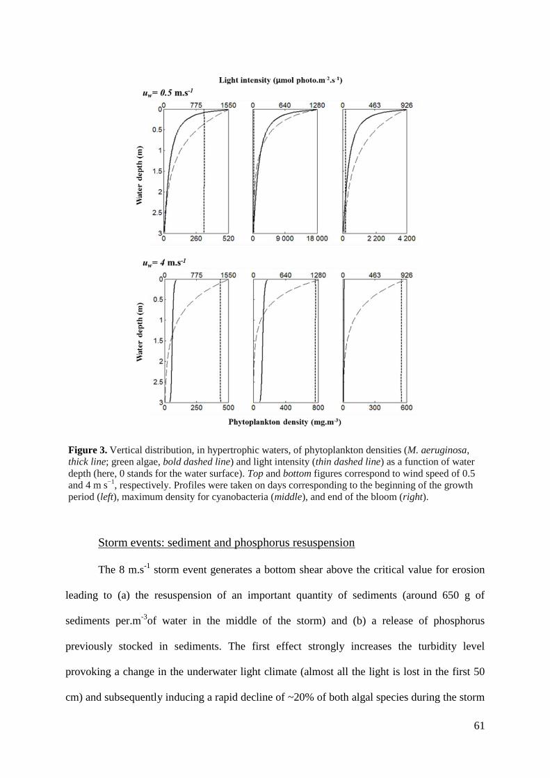
61

Storm events: sediment and phosphorus resuspension

The 8 m.s-1

storm event generates a bottom shear above the critical value for erosion

leading to (a) the resuspension of an important quantity of sediments (around 650 g of

sediments per.m-3

of water in the middle of the storm) and (b) a release of phosphorus

previously stocked in sediments. The first effect strongly increases the turbidity level

provoking a change in the underwater light climate (almost all the light is lost in the first 50

cm) and subsequently inducing a rapid decline of ~20% of both algal species during the storm

Figure 3. Vertical distribution, in hypertrophic waters, of phytoplankton densities (M. aeruginosa,

thick line; green algae, bold dashed line) and light intensity (thin dashed line) as a function of water

depth (here, 0 stands for the water surface). Top and bottom figures correspond to wind speed of 0.5

and 4 m s−1

, respectively. Profiles were taken on days corresponding to the beginning of the growth

period (left), maximum density for cyanobacteria (middle), and end of the bloom (right).

62

(Fig. 4). In the same time, the phosphorus concentration increases up to 400 mg.m-3

during the

storm.

In eutrophic waters with low regular wind exposure (Fig. 4b), the storm occurs during

the cyanobacterium peak. The subsequent phosphorus release allows M. aeruginosa to

maintain high densities longer in the season compared to simulations without any storm event.

For instance, on mid-September (Fig. 4b), M. aeruginosa mean density is around 715 mg.m-3

after the storm event to be compared to 650 mg.m-3

without storm (Fig. 2c). However, the

Figure 4. Effects of storm events (wind speed of 8 m s−1

during 2 days) on phosphorus concentration

(dashed line), densities of M. aeruginosa (thick line), and green algae (gray line). Left and right

figures display simulations for mesotrophic and eutrophic water, respectively, with storm happening

at the end of August and mid-July, respectively. a, b Data for a storm event happening in a low wind

exposure environment (0.5 m s−1

constant speed). c, d Data for a storm event happening in a medium

wind exposure environment (4 m s−1

constant speed). Arrows indicate the beginning and the end of

the storm.

63

overall dynamics is not much modified in terms of magnitude: the green algae dynamics is

very similar, which suggests that it does not benefit from the resuspended phosphorus (Fig. 4b

and 2c).

In eutrophic waters with medium regular wind exposure (Fig. 4d), the storm event

does not change the dynamics of both species except for a slightly lower global density of the

green algae after the storm compared to simulations without storm (Fig. 2d).

In mesotrophic waters with low regular wind exposure (Fig. 4a), the storm event

happens just before the beginning of the cyanobacterial development. M. aeruginosa density

reaches a maximum mean density of 1.4 103 mg.m

-3 (Fig. 4a), which is much higher than in

absence of a storm (Fig. 2a). As in eutrophic waters, the green alga does not benefit from the

storm event. Therefore, the storm event creates a favorable environment for M. aeruginosa

proliferation.

In mesotrophic waters with medium regular wind exposure (Fig. 4c), the phosphorus

release due to the storm benefits slightly to M. aeruginosa with a density reaching 100 mg.m-3

compared to simulations without storm (density at the same time around 20 mg.m-3

Fig. 2b).

It mostly benefits to the green algae that reach values comparable to simulations without

storm in eutrophic environment (Fig. 2d).

The impact of warming on the phytoplankton growth

Let us now perform simulations with higher water temperature (previous temperature

forcing increased by 2°C) in order to mimic a warmer climate (Fig. 5). The temperature

increase is favorable to the cyanobacteria and unfavorable to the green alga. But these overall

results can be strongly modulated by the wind-induced mixing.

64

For low wind speeds (0.5 m.s-1

) and mesotrophic conditions, the green algae growth is

impaired by the temperature rise and reach smaller densities throughout the season (compare

Fig. 5a and 2a). On the contrary, M. aeruginosa is favored by the temperature increase:

density reaches a maximum of 200 mg.m-3

(Fig. 5a) to be compared with the value of 38.5

mg.m-3

with standard temperatures (Fig. 2a).

For low wind speeds and eutrophic conditions, the maximal cyanobacterial density is

almost 10 times higher with warming than with standard temperatures (8.1 103 mg.m

-3 vs 784

mg.m-3

) (Fig. 5b and 2c). Moreover M. aeruginosa builds up a high density population in a

shorter time and the bloom peak occurs a few days earlier than with standard temperatures

(Fig. 5b). The phosphorus depletion by the cyanobacteria is very fast and the bloom can no

longer maintain itself despite the favorable temperatures. The decline of the bloom is also

faster than with standard temperatures. Besides, it is important to note that the green alga is

strongly suppressed during the cyanobacterial bloom, decreasing below 50 mg.m-3

at the end

of August (Fig. 5b).

For higher wind speeds (4 m.s-1

), in both mesotrophic and eutrophic situations (Fig.

5c, 5d), we observe the same trends caused by warming than those with weak winds, i.e. a

lower density of the green alga and an enhancement of M. aeruginosa compared to

simulations without warming (Fig 2b, 2d). Results show that the mixing process dampens the

effects of warming (compare figures 5a and 5c or figures 5b and 5d). M. aeruginosa displays

a decrease of its maximum density. For instance, in eutrophic and warm waters, maximum

density is reduced by 83% in wind-exposed water-column by comparison to the non-exposed

water column (Fig. 5b and 5d).

65

The mixing slightly increases the green alga density in mesotrophic conditions (Fig. 5a

and 5c), and it maintains a significant density throughout the season in eutrophic conditions

despite the development of the cyanobacterium (Fig. 5d). The dynamics of both species in

various environment conditions from July to December are detailed in figures 1-5.

The figure 6 displays, for standard temperatures (Fig. a) and 2°C increase in

temperatures (Fig. b), the logarithm of the ratio of M. aeruginosa density over the green algae

density when M. aeruginosa is at its peak (note that 0 corresponds to a ratio equal to 1). This

is done on interval of wind speeds (from 0.5 to 5 m.s-1

) and initial phosphorus concentrations

Figure 5. Effect of a 2 °C warming of the water column on phosphorus concentration (dashed

line), densities of M. aeruginosa (thick line), and green algae (gray line). Left and right figures

display simulations for mesotrophic and eutrophic water, respectively. a, b Data for 0.5 m s−1

wind speed; c, d data for 4 m s−1

wind speed.

66

(from 10 to 150 mg.m-3

). These figures show the conditions favorable for one species or the

other and what conditions lead to net dominance of one species on the other or to coexistence.

The left panel (Fig. 6a) shows that most of the wind and trophic status conditions lead

to green algae dominance or co-dominance. M. aeruginosa clear dominance is restricted to

eutrophic/hypertrophic and low wind conditions. The preference of the green algae for

medium wind exposure and low phosphorus concentrations is visible on the left of the panel

with log values below -2. In comparison, the right panel (warming, Fig. 6b) displays a clear

spread of the dominance domain of M. aeruginosa on the bottom right of the graph. This clear

dominance extends to mesotrophic conditions (~30 mg.m-3

) and higher wind speeds (~3 m.s-

1). Regions of green algae dominance shrink to the left side, where the phosphorus

concentration is very low (10-20 mg.m-3

). The top right area (log values between ~1 and ~2.5)

corresponds to M. aeruginosa dominance but with the persistence of the green algae. The

Figure 6. In the parameter plane (initial trophic status, wind), color chart of the log-transformed ratio of

M. aeruginosa density over green algae density at the precise moment when M. aeruginosa density

reaches its maximum (please note that the value of 0 on the color bar represents a ratio of 1). Left :

simulations run with standard temperatures; right: the same simulations run with a 2 °C increase in

temperatures. This figure is made from 256 simulation runs with cubic interpolation between points.

67

bottom right domain (log values above ~4) corresponds to a dense bloom with strong

limitation of the green algae growth. On both figures, especially on the right one, the green

algae dominance domain is reduced when the wind speed exceeds 4 m.s-1

. This is due to

nutrient resuspension: at those wind speeds, the pool of available phosphorus increases,

leading to favorable conditions for M. aeruginosa.

Discussion

This study proposes a model on shallow lakes which addresses the transient effects of

the interaction of physical and ecological processes, in particular storm events, on

phytoplankton dynamics. To our knowledge, it is the first to include sediment and nutrient

resuspension. Our model results stress the importance of wind effects in interactions with

trophic status and water temperature for understanding the magnitude and dynamics of M.

aeruginosa blooms.

Eutrophication and wind exposure

In accordance with field observations, our results confirm the importance of the

trophic status of a lake to understand the dominance of one algal group on another. These

results might be mechanistically supported by a difference in physiological characteristics

between phytoplankton groups. The half saturation constant of the green alga (6 mg P.m-3

) is

lower than M. aeruginosa (24 mg P.m-3

). This means that (a) in mesotrophic environment (in

the model [P]initial=20 mg.m-3

), the green alga is very much favored compared to M.

aeruginosa and therefore dominates in this environment (for this sets of temperatures); (b) in

eutrophic and hypertrophic conditions ([P]initial>65 mg.m-3

), the green alga is at its saturating

level for phosphorus while M. aeruginosa still benefits from the concentration increase,

giving it a clear advantage when temperatures become favorable. To sum up, phosphorus

concentration will condition the “carrying capacity” of the water column. Phosphorus is an

68

important driver of the competition when its level is low. At higher trophic status, other

constraints, like light availability and temperatures drive the competition. Everything being

equal, the only effect of phosphorus at higher trophic level is to accentuate the formation of

M. aeruginosa scums, which in turns reinforce its impact on underwater climate.

The buoyancy of M. aeruginosa explains its high surface density, forming dense

scums at the water surface as observed in the field (See for instance: Soranno 1997; Ahmed et

al. 2008; Homma et al. 2008). For instance our results in hypertrophic waters show a surface

density around 18 103 mg.m

-3 which is of the same order of magnitude as densities found at

the surface of water ponds by Homma et al. (2008) and Ahmed et al. (2008) (respectively 15

103 mg.m

-3 and 14.9 10

3 mg.m

-3 using a M. aeruginosa cell mass equal to 24 10

-9 mg). Despite

the small size of one M. aeruginosa cell compared to the green alga, their high surface density

in calm waters allows them to dramatically change the underwater climate and therefore

strengthen their dominance in eutrophic and hypertrophic waters. In the simulations with low

wind, the light availability under 50 cm is dramatically reduced (58% reduction in eutrophic

waters and 67% in hypertrophic waters during the blooms) impairing the development of

competitors with neutral or sinking properties. As most of M. aeruginosa population is at the

surface, it does not suffer from light limitation and therefore benefits highly from high

phosphorus availability which in turn worsens the shading due to their high density scums.

The dominance of M. aeruginosa can be altered by the wind regimes. Our results show

that a water column regularly mixed by the wind ( =4 m.s-1

) does not suffer from M.

aeruginosa blooms of the same magnitude as non-exposed ( =0.5 m.s-1

), stagnant waters.

Because of the strong water mixing, M. aeruginosa loses its capacity to colonize the surface

and the green algae take over the dominance thus creating a turbid environment impairing the

development of their competitor (Huisman et al, 2004). Therefore, the competition for light

depends strongly on the stability of the water column. These results are in accordance to those

69

of Soranno (1997) who pointed out that scums can only appear in low wind conditions. Also,

the deep-lake model developed by Huisman et al. (2004) explicitly shows that turbulence and

currents on one hand prevent M. aeruginosa from gaining the water surface and, on the other

hand, allow the sinking species to stay longer in the euphotic zone.

The wind-induced mixing allows a greater development of the green algae in all the

simulations, which is consistent with field experiments with artificial mixing (Visser et al.

1996; Ptacnik et al. 2003; Jöhnk et al. 2008; Hudnell et al. 2010b) and early modelling work

(Huisman et al. 2002b). This leads to the interesting result that, even in eutrophic and

hypertrophic conditions, a water column regularly mixed will not experience high density M.

aeruginosa blooms, as has been shown in eutrophic or hypertrophic lakes with artificial

mixing (Visser et al. 1996, Hudnell et al 2010b). These results may explain in part the

variability observed between water ponds experiencing different wind regimes according to

their location, surrounding vegetation and urbanization. Our results stress that the

presence/absence of cyanobacterial blooms do not only depend on lake trophic status. Even if

natural mixing intensity is enough to prevent blooms of buoyant species, it does not mean that

the trophic status of the lake is not high and its water quality poor.

Impacts of storm events

In this study, we distinguished two kinds of wind effects: low to medium wind speeds

that only mix the water column without disrupting the sediment surface, and high wind

speeds, i.e storm events, that induce enough bottom shear stress to induce sediment

resuspension. In our simulations, we show two distinct effects of short storm events. First, the

sediment resuspension, depending on the erodability of the soil and wind speed, strongly

decreases the light availability in the water column. As a consequence, the density of

phytoplankton species decreases rapidly. For a two days long storm, the overall

phytoplankton density is reduced by ~20%. Hellström (1991) estimated that algal production

70

was reduced by 85% when resuspension occured in the lake Tämnaren in Sweden. Second,

we observe an important increase of phosphorus concentration in the water which reaches

values around 400 mg.m-3

; this value is comparable to those obtained in resuspension

experiments (Ogilvie and Mitchell 1998). This newly available phosphorus is in part

consumed by the phytoplankton species. But the phosphorus concentration does not decrease

as fast as measured by Olgivie and Mitchell (1998). This discrepancy may be explained by the

absence in the model of 1) phosphorus sedimentation velocity and 2) phosphorus

sedimentation due to binding to the settling sediments.

The results show that, when the storm occurs during the M. aeruginosa bloom peak,

the cyanobacterial density slightly decreases but recovers readily (Fig. 4b). As explained

above, this decrease is due to increased turbidity but the cyanobacteria benefits from the

release of phosphorus from the resuspended sediments. Therefore storm events allow M.

aeruginosa to reach higher overall densities than without any storm event. In the eutrophic

shallow lake Taihu in China, Zhu et al (2005) showed that the strong and regular wind events

might be the main mode for internal release of phosphorus in the lake waters. As this lake

regularly suffers from M. aeruginosa blooms, the authors conclude that the storm events must

have important effects on the nutrient supply during blooms.

In mesotrophic waters with enriched sediments, our results show that storm events can

sufficiently change the phosphorus availability to allow the development of the cyanobacteria

(Fig. 4a). According to our simulations, those results depend on the meteorological

conditions. For instance, if regular wind exposure is rather high, and therefore not really

favorable to M. aeruginosa, it will only slightly or not at all benefit from the phosphorus

release. Conversely, it might benefit to its competitors that are doing better at higher wind

speeds. So the outcome of storm events can be strongly modulated by the general wind

exposure before and after the event.

71

Indeed, phosphorus concentration in sediments is usually high. The phosphorus pool

in the sediments can be more than 100 times higher than the pool present in the lake water

(Søndergaard et al. 2003). Besides, the quantity of phosphorus in one compartment is highly

dependent on the density in the other. This is particularly clear in lakes under restoration

plans. Even if the phosphorus input is steeply reduced, some lakes do not show any

improvement of the water quality for a considerable period after the loading reduction

(Søndergaard et al. 2003; Spears et al. 2007). Søndergaard et al. (2003) also stated that wind-

induced resuspension is a mechanism frequently causing increased sediment and phosphorus

concentrations in shallow lakes. Medium to strong mixing also allows the oxygen to be

homogeneously distributed throughout the water column, which can lead to less phosphorus

release from the sediment through complex iron-oxygen interactions (Gächter and Müller,

2003).

The model does not take into account the recruitment and flocculation of Microcystis

cells in relation to sediment. Verspagen et al. (2006) showed that aggregation to clay particles

may cause sedimentation of buoyant Microcystis. The aggregation efficiency depends on

many variables such as clay concentration and type, concentration and physiological status of

the cells. Therefore, storm events, which resuspends large amount of sediment might cause

massive sedimentation of Microcystis cells. However, storm events also affect the recruitment

of Microcystis cells living in the sediment. Verspagen et al. (2004) stated that a non-negligible

amount of Microcystis cells overwinter in sediments and stay photochemically active,

especially in shallow waters. These cells might inoculate the water column and promote the

development of blooms in summer if they can leave the sediments. Their study showed that

physiological changes (buoyancy and ballast content in cells) were unlikely to be the

recruitment cause; therefore, resuspension of sediment via mixing seems to be the most

possible recruitment mechanism.

72

Effects of warming on M. aeruginosa dominance and bloom-formation

High temperatures are usually associated with cyanobacterial blooms. Indeed,

Microcystis sp. is known to proliferate under warm climate, but also in temperate regions

during summer (Havens 2008; Jöhnk et al. 2008; Paerl & Huisman 2008; Kosten et al. 2012).

With a maximum growth rate around 28°C, M. aeruginosa is particularly adapted to summer

heatwaves and warm temperatures (Jöhnk et al. 2008). Conversely, low temperatures are also

one of the most limiting factor of M. aeruginosa development (Oberholster et al. 2004), as its

growth is critically impaired below 15°C (Jöhnk et al. 2008). The GIEC scenarios indicate

that global temperatures are rising rapidly and Rogelj et al. (2011) recently stated that if plans

to reduce global emissions are not put in place, the actual target of a 2°C increase limit will

not be achieved. Our results on the effects of a 2°C increase in water temperatures confirms

the hypothesis that rising temperatures will have a strong impact on freshwater bodies. In fact,

in eutrophic and hypertrophic conditions (results for hypertrophic conditions not shown), we

observe a strong increase in the densities reached by M. aeruginosa, an earlier bloom

formation, and also a quicker bloom die-off. In our warming simulations (with low wind), the

maximum density of Microcystis is about 10 times higher than with normal temperatures.

This trend is in accordance with other studies and observations (Jöhnk et al. 2008, Kosten et

al. 2012, Mooij et al. 2005). This is in part due to the relationship between Microcystis growth

rate vs temperature. In our simulations, with only 2°C increase in mean water temperatures,

we approach the maximum growth rate of Microcystis (about 0.8 day-1

), which allows a quick

growth of Microcystis population. However, it is important to keep in mind that our model

does not take into account natural meteorological variability, which could dampen the

importance of warming although the trend is correct.

In addition, the green alga is totally excluded in some conditions. As a consequence,

the warming worsens the effects of nutrient enrichment especially in stagnant waters. In

73

particular, we observe a cyanobacterial development even in mesotrophic conditions. The

disadvantage of M. aeruginosa in low phosphorus environment is compensated by the

increased growth rate due to high temperatures. In the field, this conclusion strongly depends

on the adaptation of the competitors to high temperatures, but Kosten et al. (2012) stated that

cyanobacteria may have higher optimum temperatures for growth than eukaryotes. Therefore,

among other well-studied negative impact of warming, such as fish kills or increased anoxic

conditions, the risk for freshwater bodies is to suffer from the loss of numerous algal species

during summer with particularly hot temperatures (Jöhnk et al. 2008). Warming also allows

the development of dense blooms at higher wind speed, but a clear limit is set around 3 m.s-1

where mixing starts to limit the maximum density reachable by M. aeruginosa. Moreover,

when the wind speed is above 3 m.s-1

the green alga maintains itself thanks to the wind

induced mixing. The wind exposure is therefore an important feature to take into account to

understand the impacts of warming on phytoplankton dynamics and diversity in shallow

lakes.

In the last decades, we saw changes in distribution and increased density of M.

aeruginosa blooms. Our predictions and recent literature (Kosten et al 2011, Jöhnk et al.

2008) indicate that the problem is worsening with rising temperatures. This is a costly

problem, from ecological and economical points of view. A lot of research has been carried to

find ways to prevent and eliminate blooms (for a review see for example Hudnell 2010a and

Gumbo et al. 2008). Chemical solutions based on algaecide are one of the mostly used

methods to suppress and terminate blooms. However, those methods are potentially dangerous

for the whole ecosystem and even favor the release of high amount of toxins from lysed

cyanobacterial cells (Touchette et al., 2008). Studies on the effect of mixing have opened new

perspectives for bloom prevention: bubbling systems have been tested in deeper lakes

suffering from Microcystis sp. blooms during the warm season (Visser et al. 1996, Jungo et al.

74

2001; Huisman et al. 2004; Jöhnk et al. 2008). The results are an efficient suppression of

blooms and algal diversity enhancement. However, those systems are costly to put in place,

need to be constantly powered and have a very limited range of action. Moreover, intermittent

use enables M. aeruginosa to develop again as soon as the system is turned off (Jöhnk et al.

2008). Another concern is that bubbling creates a transport of nutrient from the rich

hypolimnion to the epilimnion which might favor blooms (Singleton and Little 2006). Some

of those disadvantages are covered by another system called SPC (Solar Powered

Circulation), which creates a current only in the epilimnion and is powered by solar panels.

Results have been efficient bloom suppression in most of the lake tested, with the

reestablishment of a balanced algal community years after the deployment (Hudnell et al.

2010b). So the question is: are those systems adaptable to shallow lakes? In Hudnell et al.

(2010b) experiments, the SPC system failed in very shallow lakes where fish densities,

affluents carrying cyanobacteria and other factors might have overcome or counteract the

effect of mixing (Hudnell et al. 2010b). Our study points out another difficulty: mixing in

shallow lakes may disrupt the sediment surface and enhance phosphorus release as shown in

our simulations with storm events. Adapting this technic to shallow lakes (< 1m depth) might

prove to be risky and uncertain.

Conclusion

In shallow lakes, wind has a key role in the structure and dynamic of phytoplankton

populations. By mixing the water column and inducing sediment and nutrient resuspension, it

affects strongly the competition for light and nutrients. Regular mixing by medium wind

prevents the development of the buoyant M. aeruginosa. Punctual storm events have two

successive effects: 1) a global decrease in phytoplankton density due to increased turbidity, 2)

species can benefit from the phosphorus release by sediments depending on the timing of the

event and the general wind exposure. The consequences of a 2°C warming are an earlier and a

75

denser M. aeruginosa bloom in summer and blooms in mesotrophic waters. However, the

symptoms of warming can be masked by the wind-regime experienced by the lake. The

interactions between eutrophication, warming and wind regimes may produce unexpected

effects on cyanobacterial dynamics in shallow lakes.

Acknowledgments

L.B thanks G. Hmimina for his help in improving the figures quality. We thank the reviewers

for their comments which strongly improved the manuscript quality. L.B. and this work are

financially supported by the ANR Pulse 2010 CEPL 01004. F.M was supported by a post-

doctoral grant from the University Pierre et Marie Curie (Paris, France).

References

Ahmed MS, Hiller S, Luckas B (2008) Microcystis aeruginosa Bloom and the Occurrence of

Microcystins (Heptapeptides Hepatotoxins ) From an Aquaculture Pond in Gazipur ,

Bangladesh. Turk J Fish Aquat Sci 41:37–41.

Baldia SF, Evangelista a. D, Aralar E V., Santiago a. E (2007) Nitrogen and phosphorus

utilization in the cyanobacterium Microcystis aeruginosa isolated from Laguna de Bay,

Philippines. J Appl Phycol 19:607–613

Bengtsson L, Hellstrom T (1992) Wind-induced resuspension in a small shallow lake.

Hydrobiologia 241:163–172

Bonnet M., Poulin M (2002) Numerical modelling of the planktonic succession in a nutrient-

rich reservoir: environmental and physiological factors leading to Microcystis

aeruginosa dominance. Ecol Model 156:93–112

Carmichael WW, Azevedo SM, An JS, Molica RJ, Jochimsen EM, Lau S, Rinehart KL, Shaw

GR, Eaglesham GK (2001) Human fatalities from cyanobacteria: chemical and

biological evidence for cyanotoxins. Env Health Persp 109:663–668.

CERC (1984) Shore protection manual, vol.1. Vicksburg, MS, USA: US Army Corp of

517 Engineering

Chao X, Jia Y, Shieldsjr F, Wang S, Cooper C (2008) Three-dimensional numerical modeling

of cohesive sediment transport and wind wave impact in a shallow oxbow lake. Adv

Water Res 31:1004–1014

76

Chen Y, Fan C, Teubner K, Dokulil M (2003) Changes of nutrients and phytoplankton

chlorophyll-a in a large shallow lake , Taihu , China : an 8-year investigation.

Methods:273–279

Chen Y, Qin B, Teubner K, Dokulil M (2003) Long-term dynamics of phytoplankton

assemblages : Microcystis-domination in Lake Taihu , a large shallow lake in China. J

Plankton Res 25:445–453

Codd GA, Bell SG, Kaya K, Ward CJ, Beattie KA, Metcalf JS (1999) Cyanobacterial toxins,

exposure routes and human health. Eur J Phycol 34:405–415

De Figueiredo DR, Azeiteiro UM, Esteves SM, Gonçalves FJM, Pereira MJ (2004)

Microcystin-producing blooms : a serious global public health issue. Ecotox Environ

Safe 59:151–63

Downing JA, Watson SB, McCauley E (2001) Predicting cyanobacteria dominance in lakes.

Can J Fish Aquat Sci 58:1905–1908

Elliott JA, Jones ID, Thackeray SJ (2006) Testing the Sensitivity of Phytoplankton

Communities to Changes in Water Temperature and Nutrient Load, in a Temperate Lake.

Hydrobiologia 559:401–411

Elliott AJ, May L (2008) The sensitivity of phytoplankton in Loch Leven (U.K.) to changes in

nutrient load and water temperature. Fresh Biol 53:2–41

Falconer IR, Humpage AR (2005) Health risk assessment of cyanobacterial (blue-green algal)

toxins in drinking water. Int J Environ Res Public Health 2:43–50

Gächter R, Müller B (2003) Why the phosphorus retention of lakes does not necessarily

depend on the oxygen supply to their sediment surface. Limnol Oceanogr 48:929–933

Graham LE, Wilcox LW (2000) Algae. Prentice Hall, Upper Saddle River, New Jersey; 2000

Gumbo RJ, Ross G, Cloete ET (2008) Biological control of Microcystis dominated harmful

algal blooms. Afr J Biotechnol 7:4765-4773

Havens KE (2008) Cyanobacteria blooms: effects on aquatic ecosystems. Adv Exp Med Biol

619:733–747

Hellström T (1991) The effect of resuspension on algal production in a shallow lake.

Hydrobiologia 213, 183-190

Homma T, Komatsu N, Negishi M, Katagami Y, Nakamura K (2008) Influence of Dissolved

Inorganic Nitrogen and Phosphorus Concentrations on the Horizontal and Temporal

Changes of Microcystis Population in Lake. M. Sengupta, R. Dalwani (Eds.),

Proceedings of Taal2007: The 12th World Lake Conference (2008) 1423–1429

Hudnell HK. (2010a) The state of U.S. freshwater harmful algal blooms assessments, policy

and legislation. Toxicon 55, 1024-34

77

Hudnell HK, Jones C, Labisi , Lucero V, Hill DR, Eilers J (2010b) Freshwater harmful algal

bloom (FHAB) suppression with solar powered circulation (SPC). Harmful Algae

9:208–217

Huisman J, Weissing FJ (1994) Light-Limited Growth and Competition for Light in Well-

Mixed Aquatic Environments: An Elementary Model. Ecology 75:507–520

Huisman J, Van Oostveen P, Weissing FJ (1999a). Critical Depth and Critical Turbulence :

Two Different Mechanisms for the Development of Phytoplankton Blooms. Limnol

Oceanogr 44:1781–1787

Huisman J, Van Oostveen P, Weissing FJ (1999b) Species Dynamics in Phytoplankton

Blooms: Incomplete Mixing and Competition for Light. Am Nat 154:46–68

Huisman J, Sommeijer B (2002a) Population dynamics of sinking phytoplankton in light-

limited environments: simulation techniques and critical parameters. J Sea Res 48:83–96

Huisman, J, Arrayás M, Ebert U, Sommeijer B (2002b). How do sinking phytoplankton

species manage to persist? Am Nat 159:245–54

Huisman J, Sharples J, Stroom JM, Visser PM, Kardinaal WE, Verspagen JMH, Sommeijer B

(2004) Changes in Turbulent Mixing Shift Competition for Light Between

Phytoplankton Species. Ecology 85:2960–2970

Jacoby JM, Collier DC, Welch EB, Hardy FJ, Crayton M (2000) Environmental factors

associated with a toxic bloom of Microcystis aeruginosa. Can J Fish Aquat Sci 57:231–

240

Jöhnk KD, Huisman J, Sharples J, Sommeijer B, Visser PM, Stroom JM (2008) Summer

heatwaves promote blooms of harmful cyanobacteria. Glob Change Biol 14:495–512

Jungo E, Visser PM, Stroom J, Mur LR (2001) Artificial mixing to reduce growth of the blue-

green alga Microcystis in Lake Nieuwe Meer, Amsterdam: an evaluation of 7 years of

experience. Water Sci Technol 1:17–23

Klausmeier C and Litchman E (2001) Algal games: The vertical distribution of phytoplankton

in poorly mixed water columns. Limnol Oceanogr 46:1998–2007

Kosten S, Huszar VLM, Bécares E, Costa LS, Donk E, Hansson L-A, Jeppesen E, Kruk C,

Lacerot G, Mazzeo N, Meester L, Moss B, Lürling M, Nõges T, Romo S, Scheffer M

(2012) Warmer climates boost cyanobacterial dominance in shallow lakes. Glob Change

Biol 12:118–126

Luettich RA, Harleman DR, Somlyody L (1990) Dynamic behavior of suspended sediment

concentrations in a shallow lake perturbed by episodic wind events. Limnol Oceanogr

35:1050–1067

Moss B, Mckee D, Atkinson D, Collings SE, Eaton JW, Gill a. B, Harvey I, Hatton K, Heyes

T, Wilson D (2003) How important is climate? Effects of warming, nutrient addition and

fish on phytoplankton in shallow lake microcosms. J. Appl. Ecol. 40:782–792

78

Mooij WM, Hülsmann S, De Senerpont Domis LN, Nolet BA, Bodelier PLE, Boers PCM,

Pires LMD, Gons HJ, Ibelings BW, Noordhuis R, Portielje R, Wolfstein K., Lammens

EHRR (2005) The impact of climate change on lakes in the Netherlands: a review.

Aquat. Ecol. 39:381–400

Oberholster PJ, Botha A-M, Grobbelaar JU (2004) Microcystis aeruginosa : source of toxic

microcystins in drinking water. Afr. J. Biotechnol. 3:159–168

Ogilvie BG, Mitchell SF (1998) Does sediment resuspension have persistent effects on

phytoplankton ? Experimental studies in three shallow lakes. Fresh Biol 40:51–63

Ptacnik R, Diehl S, Berger S (2003) Performance of sinking and nonsinking phytoplankton

taxa in a gradient of mixing depths. Limnol Oceanogr 48:1903–1912

Paerl HW (1988) Nuisance phytoplankton blooms in coastal, estuarine, and inland waters.

Limnol Oceanogr 33:823–847

Paerl HW, Huisman J (2008) Blooms Like It Hot. Science 320:57–58

Qin B (2004) Dynamics of sediment resuspension and the conceptual schema of nutrient

release in the large shallow Lake Taihu, China. Chinese Sci Bull 49:54–64

Reynolds CS (2006) Ecology of freshwater phytoplankton. Cambridge University Press,

Cambridge

Rogelj J, Hare W, Lowe J, van Vuuren DP, Riahi K, Matthews B, Hanaoka T, Jiang K,

Meinshausen M (2011) Emission pathways consistent with a 2 °C global temperature

limit. Nature Clim. Change 1:413–418

Singleton VL, Little JC (2006) Designing hypolimnetic aeration and oxygenation systems – a

review. Environ. Sci. Technol 40:7512–7520.

Søndergaard M, Jensen JP, Jeppesen E (2003) Role of sediment and internal loading of

phosphorus in shallow lakes. Hydrobiologia 506-509:135–145

Soranno P (1997) Factors affecting the timing of surface scum and epilimnetic blooms of

blue-green algae in a eutrophic lake. Canadian Journal of Fisheries and Aquatic Sciences

54:1965–1975

Scheffer M (1998) Ecology of shallow lakes. Chapman and Hall, London

Sommer U, Adrian R, De Senerpont Domis L, Elser JJ, Gaedke U, Ibelings B, Jeppesen E,

Lürling M, Carlos Molinero J, Mooij WM, van Donk E, Winder M (2012) Beyond the

Plankton Ecology Group (PEG) Model: Mechanisms Driving Plankton Succession. Annu

Rev Ecol Evol Syst 43:429–48

Spears BM, Carvalho L, Paterson DM (2007) Phosphorus partitioning in a shallow lake:

implications for water quality management. Water Environ. J. 21:47–53

79

Teeter AM, Johnson BH, Berger C, Stelling G, Scheffner NW, Garcia MH, Parchure TM

(2001) Hydrodynamic and sediment transport modeling with emphasis on shallow-water,

vegetated areas (lakes, reservoirs, estuaries and lagoons). Hydrobiologia 444:1–23

Touchette BW, Edwards CT, Alexander J (2008) A comparison of cyanotoxin release

following bloom treatment with copper sulfate or sodium carbonate perohydrate. In:

Hudnell HK (Ed.) Cyanobacterial Harmful Algal Blooms: State of the Science and

Research Needs, Adv Exp Med Biol 619 Chapter 14. Springer Press, New York, pp.314–

315

Verspagen JMH, Snelder EOFM, Visser PM, Huisman J, Mur LR, Ibelings BW (2004)

Recruitment of Benthic Microcystis (Cyanophyceae) To the Water Column: Internal

Buoyancy Changes or Resuspension? J Phycol 40:260–270

Verspagen JMH, Visser PM, Huisman J (2006) Aggregation with clay causes sedimentation

of the buoyant cyanobacteria Microcystis spp.Aquat Microb Ecol 44:165–174

Visser P, Ibelings B, Van Der Veer B, Koedood J, Mur R (1996) Artificial mixing prevents

nuisance blooms of the cyanobacterium Microcystis in Lake Nieuwe Meer, the

Netherlands. Fresh Biol 36:435–450

Wiegand C, Pflugmacher S (2005) Ecotoxicological effects of selected cyanobacterial

secondary metabolites: a short review. Toxicol Appl Pharmacol 203:201–218

Wu J and Tsanis IK (1995) Numerical study of wind-induced water currents. J Hydrau Eng

121:388–395

Yoshiyama K, Mellard JP, Litchman E, Klausmeier CA (2009) Phytoplankton competition for

nutrients and light in a stratified water column. Am Nat 174:190–203

Zegura B, Sedmak B, Filipic M (2003) Microcystin-LR induces oxidative DNA damage in

621 human hepatoma cell line HepG2. Toxicon 41:41–48

Zhu G, Qin B, Guang G (2005) Direct evidence of phosphorus outbreak release from

sediment to overlying water in a large shallow lake caused by strong wind wave

disturbance. Chinese Sci Bull 50:577–582

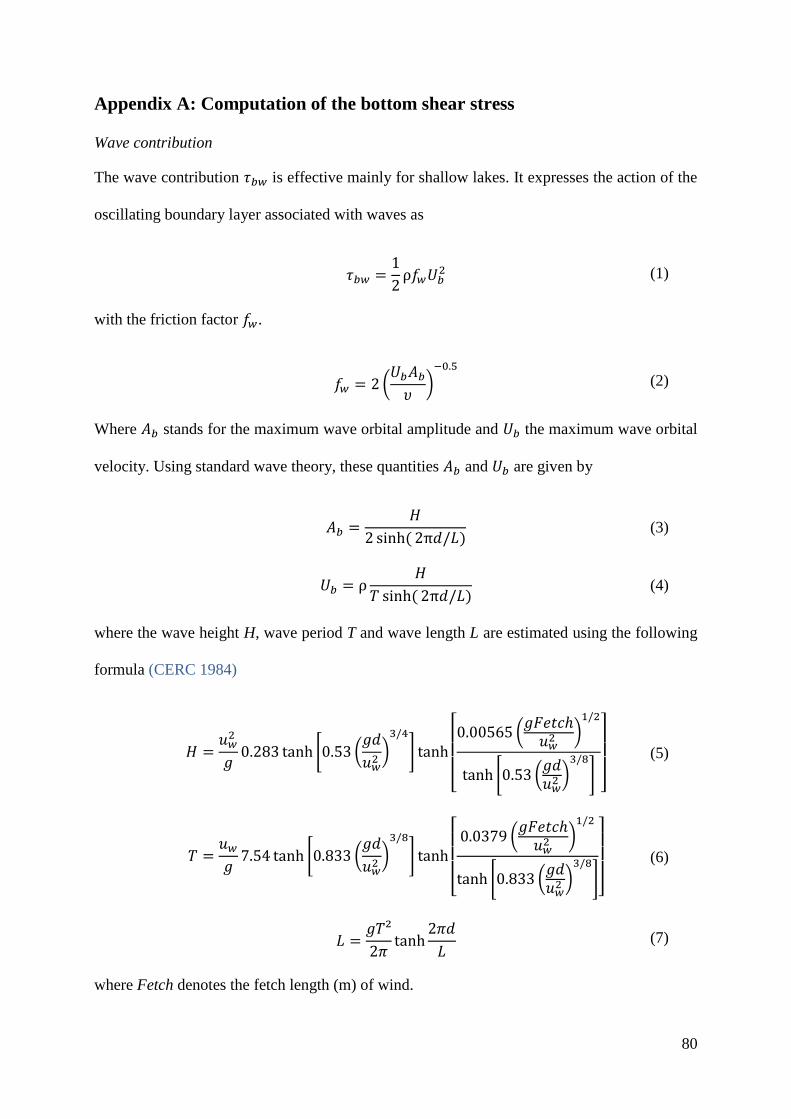
80

Appendix A: Computation of the bottom shear stress

Wave contribution

The wave contribution is effective mainly for shallow lakes. It expresses the action of the

oscillating boundary layer associated with waves as

(1)

with the friction factor .

(

)

(2)

Where stands for the maximum wave orbital amplitude and the maximum wave orbital

velocity. Using standard wave theory, these quantities and are given by

(3)

(4)

where the wave height H, wave period T and wave length L are estimated using the following

formula (CERC 1984)

* (

)

+

[ (

)

* (

)

+]

(5)

* (

)

+

[ (

)

* (

)

+]

(6)

(7)

where Fetch denotes the fetch length (m) of wind.

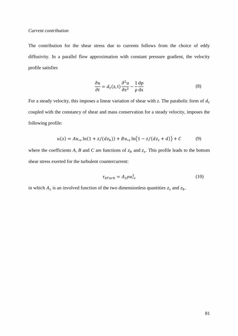
81

Current contribution

The contribution for the shear stress due to currents follows from the choice of eddy

diffusivity. In a parallel flow approximation with constant pressure gradient, the velocity

profile satisfies

(8)

For a steady velocity, this imposes a linear variation of shear with z. The parabolic form of

coupled with the constancy of shear and mass conservation for a steady velocity, imposes the

following profile:

( ) (9)

where the coefficients A, B and C are functions of and . This profile leads to the bottom

shear stress exerted for the turbulent countercurrent:

(10)

in which is an involved function of the two dimensionless quantities and .

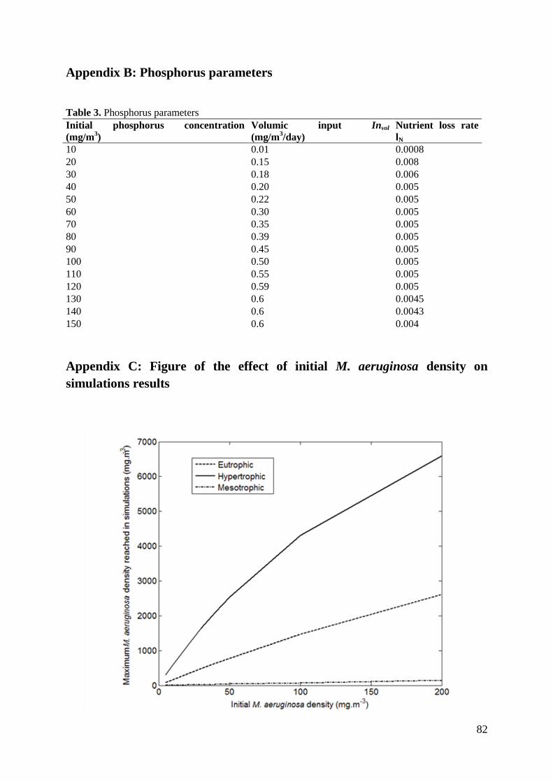
82

Appendix B: Phosphorus parameters

Appendix C: Figure of the effect of initial M. aeruginosa density on

simulations results

Table 3. Phosphorus parameters

Initial phosphorus concentration

(mg/m3)

Volumic input Invol

(mg/m3/day)

Nutrient loss rate

lN

10 0.01 0.0008

20 0.15 0.008

30 0.18 0.006

40 0.20 0.005

50 0.22 0.005

60 0.30 0.005

70 0.35 0.005

80 0.39 0.005

90 0.45 0.005

100 0.50 0.005

110 0.55 0.005

120 0.59 0.005

130 0.6 0.0045

140 0.6 0.0043

150 0.6 0.004

83

Appendix D: Figure of the percentage of light lost for all depths and dates

of the figure 3.

84

85

Chapter II

86

87

Mesocosms with wavemakers: a new device to study the effects

of water-mixing on lake ecology

Florence D. Hulot, Maurice Rossi, Bruno Verdier, Jean-Pascal Urban, Lydie Blottière,

Fantina Madricardo and Beatriz Decencière

In preparation for submission to Limnology & Oceanography: Methods

88

Abstract

Water structuration, either by wind or by solar radiation, is a physical characteristic of

aquatic ecosystems. Wind forcing is a transfer of energy to the water, which responds with

currents, surface and internal waves that greatly influence chemical parameters and food web

dynamics (Wetzel 2001). In order to manage freshwater ecosystems, different devices have

been developed to modify lake‟s physical structure. Other studies seek to emulate some

physical processes in experimental systems. Here we review succinctly these experimental

works. Most devices generate turbulence flows that are a particular flow regime characterized

by chaotic changes in properties. They do not reproduce precisely natural physical processes

occurring in lakes but seek to emulate them. By contrast, surface and internal waves,

generated by wind, affect the surface of the water and induce circular motions of water

particles with a slow horizontal displacement of water and orbital motions of water particles

in the water column. In fluid mechanics, the study of fluid motions under different forces

stimulated the development of different experimental designs. Tanks with wave or tidal

generators are common devices installed to reproduce natural processes and are used for

research or applied purposes. To better understand the interaction between the physical and

biological properties of aquatic ecosystems, one may want to reproduce predictable water

motions. Indeed the importance of surface waves on the lake functioning justifies the

development of a device designed to reproduce the effects of wind forcing. In this paper, we

present new original 15 m3 mesocoms with wavemakers designed to reproduce the effects

surface and internal waves. We detail the theoretical effects of waves on the water column

and the choices that have been made to design our device.

89

Introduction

Water motions are of primary importance for aquatic ecosystems functioning.

Common thought sese the water column as spatially homogeneous system except for the

summer and winter stratifications (Wetzel 2001). Water masses however are submitted to

inhomogeneous turbulence and surface and internal waves that greatly influence chemical

parameters and food web dynamics (Reynolds 2006; Scheffer 1998; Wetzel 2001). Studying

the interactions between the physical and the ecological structures of aquatic ecosystems

needs specific experimental systems. The aim of this paper is to present a new experimental

system for freshwater ecology that generates surface waves whose effects propagate in the

water column. First we introduce the importance of physical characteristics for ecosystems

and the effects of wind forcing on lake physical structure. Second we review succinctly

experimental systems that have been developed to modify the physical structure of freshwater

ecosystems in real lakes or in mesocosms, either to study them or for management purposes.

We then focus on surface and internal waves and their effects on deep and shallow lakes. We

finally give the underlying theory and describe the original experimental system.

Physical characteristics, wind forcing and water motions in lakes

Following the definition of Tansley (1935) that is still widely accepted (Gignoux et al. 2011),

an ecosystem is the union of two components, a physical system and a biological system. The

study and management of ecosystems may either focus on one of these two systems or

consider them as indivisible parts of one system (For a discussion on the definition of

ecosystem, see Gignoux et al. 2011). For instance, the experimental studies of nutrient

enrichment on food web dynamics explore how the change of a chemical factor affects the

biological system with a focus on energy and matter flows. In these studies, the physical

system may be either the habitat, i.e. the physical container characterized by a set of fixed

90

variables, or else the arena, i.e. the place with unsteady characteristics in which organisms

interact. In this context, the physical system is not the focus of the study and it has the the

underlying hypothesis that the biological system is driven by a physical factor. By contrast, in

other studies, the ecosystem is defined as a dual object by nature and physics and biology are

aspects, rather than components, and they can affect each other (Gignoux et al. 2011). This

approach has been fruitful for the study of Microcystis aeruginosa, a cyanobacteria that forms

dense blooms in freshwater (Blottière et al. 2014). Thanks to gas vesicles that increase cell

buoyancy, these cyanobacteria flows up to the surface and may outcompete other

photosynthetic organisms by changing a physical parameter, the light climate in the water

column. The buoyancy is a physical competitive advantage as surface cells shade the water

column. However this competitive advantage depends on a major physical factor, water

mixing by wind forcing. Either water is not well-mixed by wind forcing and still water allows

the expression of the buoyant characteristics of M. aeruginosa cells; or water is well-mixed by

wind forcing and the cells lose their competitive advantage for light as they are dispersed in

the water column. The study of the dual nature of the ecosystem implies the development of

adapted systems when studying or managing them.

The physical state of a lake, temperature and chemical stratifications for instance, is

modified by external forces that derive from energy or matter exchanges at its boundaries.

The main exchange arises from the wind stress and the thermal energy input by solar radiation

or evaporation. Other main processes that affect the lake physical states are inputs and outputs

of water and matter from rivers and groundwater tables. Wind forcing is a transfer of energy

to the water, which responds with currents, surface and internal waves that generate large

scale flows as well as turbulent motions. This transfer depends on (1) the fetch, the lake

distance to leeward, (2) the morphometry, that is the lake surface:volume ratio and shape, and

(3) the stratification, the thermic structure defined by solar radiation.

91

Coherent water motions induced by wind forcing in lakes appear at different spatial

scales: large scale surface or internal seiches, internal waves, surface (or progressive) waves

and Langmuir circulations. Seiches appear after long-standing winds in a constant direction.

As a consequence water piles up at one end of the lake and, when the wind stops, the water

flows back to equilibrium with a rocking motion of the entire water mass. Seiches affect the

motion of the entire water mass. Internal waves are smaller scale structures but are long

enough to affect the metalimnion and the lake bottom. Surface waves affect only the surface

of the water. Finally Langmuir circulation is a vortex, which arises through the interaction of

a drift induced by surface wave and the presence of a vertical shear in turbulent fluid (Thorpe

2004). These different flows are characterised by large scale current structures and not simply

small scale turbulence.

Small scale turbulence in lakes results from different processes: mainly natural

convection at the surface, breaking of internal waves and shear. Vertical shear may take place

at the surface, at the pycnocline and at the bottom and generates turbulences through various

instability processes (Kelvin-Helmholtz instability, boundary layer instability, for instance).

Experimental devices manipulating the water-column structuration

In order to study or manage freshwater ecosystems, different devices have been

developed to modify lake‟s spatial structure. The Table 1 summarizes the operating principles

of these devices and the physical processes involved. The objectives in management are to

improve water quality, that is in most of the cases to obtain the lake destratification to

alleviate problems linked to bloom-forming cyanobacteria (Burford and O‟donohue 2006;

Hawkins and Griffiths 1993; Hudnell et al. 2010; Oberholster et al. 2006; Steinberg 1983;

Upadhyay et al. 2013; Visser et al. 1996). The objectives in research encompass the study of

mixing depth and background turbidity on phytoplankton species (Diehl et al. 2002), the

92

effects of destratification and water column-mixing on bacteria and plankton (Becker et al.

2006; Read et al. 2011; Reynolds et al. 1983; Weithoff et al. 2000) and the effects of sediment

resuspension on phytoplankton biomass and plant nutrient concentration (Ogilvie and

Mitchell 1998). The operating principles of the devices can be split in five categories (Table

1): (1) bubble plume or air bubble curtail that generates a mixed water layer; (2) long-distance

circulation of the epilimnion that disrupts the quiescent surface water or deepens the

epilimnion; (3) up and down water motions that increase high-frequency internal waves and

generate turbulences; (4) air-providing tubs that generate turbulence; and (5) manual mixing

that also generates turbulences in water-column. All these devices aim to modify the water-

column structuration, i.e. destratification, but do not seek to reproduce natural physical

processes occurring in lakes. Most of the devices generate turbulent flows that have a

particular flow regime characterized by chaotic properties changes. However, in order to

better understand the interaction between the physical and biological properties of aquatic

ecosystems, it is necessary to reproduce predictable water motions.

Effects of waves in deep and shallow lakes

The shear stress produced by wind at the water surface generates traveling

(progressive) surface waves as well as internal waves. These waves induce orbital motions of

water particles (Figure 1A). Surface waves have an effect on mixing only at the water surface.

Internal waves whose amplitude is maximum near the pycnocline possess much larger

wavelength and are much slower. According to the ratio between the lake depth d and the

wave wavelength λ of internal waves, the effects on the water column are very different.

When the lake is deep that is to say the wave wavelength is small relative to the lake depth,

the shear at the bottom boundary is negligeable. When the lake is shallow that is the internal

wave wavelength is long compared to the depth, the orbital motions of water particles reach

93

Table 1. Review of the systems developed to modify lake’s spatial structure

Operating principles Processes involved References

Bubble plume or air bubble curtails. Long diffuser-

pipe with nozzles connected to an off-shore compressor

with an air-providing pipe.

Generation of turbulence in the water column

creating a mixed water layer, possibly below a thin

warm surface layer not affected by the turbulence

Becker et al (2006); Burford

and O‟Donohue (2006);

Hawkins and Griffiths (1993);

Oberholster et al (2006);

Visser et al (1996)

Long-distances circulation of the epilimnion. Flexible

intake hose attached to the base of a (solar-powered)

impeller with an intake depth usually above the

thermocline for epilimnion circulation or air lift apparatus

that discharges water through airlift.

Turbulent mixing with deep epilimnion water

pumping and disruption of quiescent surface water

or deepening of the epilimnion by drawing

hypolimnetic water and discharging it into the

epilimnion.

Hudnell et al (2010); Reynolds

et al (1983) ; Upadhyay et al

(2013)

Up and down water motions. 8.25 m diameter rubber

membrane surrounded by a buoyancy-controlled ring that

can be raised and lowered repeatedly through the water

column using compressed air (Gradual Entrainment Lake

Inverter [GELI])

Up and down motions (1) increase high-frequency

internal waves, (2) generate shear stress in the water

column and turbulence and (3) generates turbulence

with cold water lifted by the GELI spreading at the

surface.

Read et al (2011)

Air providing tub. Air-providing tub connected at one

end to a compressor, which pumps regularly air, and to a

diffusor to the other end situated at the deepest part of a

lake basin or at the bottom end of an enclosure.

Generation of turbulence in the water column Diehl et al (2002) ; Steinberg

(1983)

Manual mixing (small scale). Water mixing with a

wooden oar or mixing by vertically hauling a 60-cm

diameter metal plate in 1.5 m diameter enclosures

Generation of turbulence in the water column and

vertical flows generated by the vertical motions of

the metal plate

Ogilvie and Mitchell (1998);

Weithoff et al (2000)

94

the benthic zones and are able to generate a stress at the bottom boundary. If the resistance of

the bottom substrate is low in relation to the flow speed, sediments may be resuspended in the

water column (Niemisto et al. 2008; Kleeberg and Herzog, 2014). The effects of waves are

hence of particular importance in lakes. Interactions between the benthic, pelagic and littoral

zones form the core of the functioning of these ecosystems (Scheffer 1998). The effects of

waves on freshwater column mixing have been widely studied in deep lakes in order to

understand the relationship between sinking and non-sinking phytoplankton (Diehl et al.

2002; Huisman et al. 1999a; Huisman et al. 1999b).

95

Mesocosms with wavemakers: a new ecological device

The importance of internal waves on the lake functioning justifies the development of

a device designed to reproduce the effects of this wind forcing. Tanks with wave makers are

common devices installed to reproduce natural processes and are used for research or applied

purposes. For instance, different wave and swell makers have been designed worldwide by

national navies for testing model warships and measuring their wave drag. (Fascinating

pictures and movies can be found on the worldwide web.) The functioning of a tank with a

wavemaker is well known (see for a short history Hyun 1976) and the originality of our

system relies in the adaptation for research in freshwater ecology. The principle of our device

is to emulate in a mesocosm internal waves with surface waves generated by the wavemaker.

Next paragraph, we describe the effect of surface waves on the water column and explain the

choices that have been made to design our device.

Theoretical background

Progressive surface wave are characterized by the displacement in time and space of a

point at the water surface. This displacement induces a distortion ζ of the surface described as

follows:

(1)

Where x and t are the space and time dimensions, a is the wave amplitude (2a is the distance

between the wave‟s trough and crest), , is the wave number with λ the wave

wavelength (the distance between two crests), and ω the wave temporal frequency.

The classical theory gives the general propagation velocity of surface waves:

(

) (2)

where h is water depth and g is the gravity,

and the velocity of a water particles at a depth z:

96

- Horizontal component: [ ]

(3)

- Vertical component: [ ]

(4)

The equations (3-4) show that 1) the velocity of a water particle decreases with depth, and 2)

the decrease with depth is a function of the wave‟s wavelength.

When two waves of identical frequency but traveling opposite directions in the same

medium encounter each other, they interfere with one another and the result of the

interference is a new wave described as standing or stationary wave. This superposition of

two individual waves occurs in tank with vertical edges where progressive waves bounce,

travel back and encounter newly generated progressive waves. Standing waves are described

as follow by the classical theory:

- the distortion ζ of the surface is (5)

and the velocity of a water particles at a depth z:

- Horizontal component: [ ]

(6)

- Vertical component: [ ]

(7)

The classical theory allows us to describe water particle motions according to water

depth in shallow and deep waters where the ratio water depth:wavelength is small or large

respectively (Figure 1, Table 2). With progressive waves, In deep lakes, the motions are

orbital and the velocity decrease with depth and, below a depth of around ⁄ , their effects

become negligible. In shallow lakes, water particle motions become ellipsoidal, their

amplitude decreases slowly and are constant for very shallow water ( ⁄ ), and they

may provoke a shear stress at the bottom boundary. With standing waves, water particle

motions have the same pattern in deep lake than with progressive waves. In shallow lakes,

motions are ellipsoidal but not flat as with progressive waves.

97

The aim of developing mesocosms with wavemakers is to reproduce the effects of

internal waves with different wave amplitude, number and frequency and see their effects on

the water column. The theory for wavemakers has been developed by Hyun (1976). We report

here the characteristics of our system. Most tanks use one of the two types of wavemakers

called after the motion of the oscillating paddle: either flap or piston. In the flap wavemaker,

the paddle rotates around an axis assembled at its basis (Figure 2). Paddle oscillations

generate at the surface orbital motions of water particles that decay with depth. With piston

wavemaker, the paddle slides and generates elliptical motions of water particle at all depth.

Flap wavemakers are better adapted to reproduce waves in a deep water column while piston

wavemakers reproduce water motions in shallow water column. However, the effects of flap

wavemakers on the water column depend on the ratio water depth:wavelength as detailed

above and they may generate ellipsoidal water particle motions at the bottom if the parameters

(see below) are set to get a small ratio. We choose to develop a flap wavemaker because it is

more flexible for the type of effects it may generate.

Figure 2.Schematic representation of a mesocosm with a wave-generator.The tank is rectangular with a

wave-generator a one end. The engine is the light-grey box and the paddle is the dark-grey plane.

Dimensions are indicated on the diagram but water depth cannot exceed 1 m.

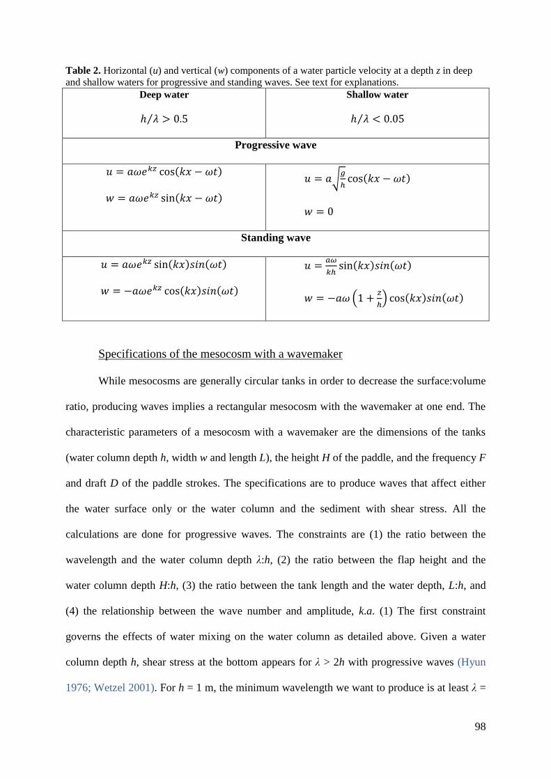
98

Table 2. Horizontal (u) and vertical (w) components of a water particle velocity at a depth z in deep

and shallow waters for progressive and standing waves. See text for explanations.

Deep water

⁄

Shallow water

< ⁄

Progressive wave

√

Standing wave

(

)

Specifications of the mesocosm with a wavemaker

While mesocosms are generally circular tanks in order to decrease the surface:volume

ratio, producing waves implies a rectangular mesocosm with the wavemaker at one end. The

characteristic parameters of a mesocosm with a wavemaker are the dimensions of the tanks

(water column depth h, width w and length L), the height H of the paddle, and the frequency F

and draft D of the paddle strokes. The specifications are to produce waves that affect either

the water surface only or the water column and the sediment with shear stress. All the

calculations are done for progressive waves. The constraints are (1) the ratio between the

wavelength and the water column depth λ:h, (2) the ratio between the flap height and the

water column depth H:h, (3) the ratio between the tank length and the water depth, L:h, and

(4) the relationship between the wave number and amplitude, k.a. (1) The first constraint

governs the effects of water mixing on the water column as detailed above. Given a water

column depth h, shear stress at the bottom appears for λ > 2h with progressive waves (Hyun

1976; Wetzel 2001). For h = 1 m, the minimum wavelength we want to produce is at least λ =

99

2 m. (2) The second constraint governs the paddle size relative to the water depth. Generating

waves induces hydrodynamically induced torque and hydrodynamic force on the flap that we

want to minimize. These physical effects decrease with an increase of the λ:h ratio, and

increase with the H:h ratio (Hyun 1976). The maximum value of the ratio is 1 when the

paddle height equals the water depth. Reducing the ratio implies reducing the height of the

paddle and fixing it at the corresponding height of the tank. For instance, a ratio of 0.5 or 0.25

implies fixing the paddle at mid-height or quarter-height of the tank respectively. However,

attaching a small paddle on the top of the tank precludes experiments with a small water

depth. Therefore, we set the H:h ratio to 1. (3) The third constraint governs the water column

distortion by spatially transitory perturbations near the wavemaker. These perturbations decay

rapidly and virtually disappear after traveling a distance of 3h (Hyun 1976). (4) The fourth

constraint governs the crest formation and wave breaking. To observe the effects of surface

waves, we want to avoid wave breaking that generates turbulences. This is insured when

ka<0.1, that is ⁄ < . Taking into account all these constraints lead to a tank of a

length L = 10 m, a width w = 1.5 m, and a height of 1.5 m for a water column 0.6 m ≤ h ≤1 m.

The maximum water volume is 15 m3. The paddle height, draft and frequency are respectively

H = 1.2 m, 0 mm ≤ D ≤ 60 mm at 1 m height and 0.21 Hz ≤ F ≤ 1.5 Hz. Hence in normal use,

the wavemaker may produce waves with a wavelength between 0.06 and 3.6 m and a

maximum amplitude of 60 mm at a maximum water column of 1 m.

Technical study of a prototype

A prototype was developed with a collaboration of the Aissor firm and tested at the

CEREEP Ecotron IleDeFrance (Saint-Pierre-lès-Nemours, France) during Spring 2011

(Figure 3). We show here results about the effect of waves‟ wavelength and amplitude on

water circulation in the water column with standing waves. We explored the wave generator

100

parameters that is the frequency of paddle stroke and its draft angle, and the produced waves

that do not break. The water velocity was measured with an Acoustic Doppler Velocimeter

(MicroADV 16 MHz, Aqualyse) at different depth in a mesocosm where the water height was

1 m. Because surface waves induce a circular motion of water particles, their mean velocity is

close to null and their standard deviation changes with waves‟ wavelength and amplitude. As

detailed above, waves with a large amplitude and wave number form crests and break. Wave

number is inversely related to wave wavelength. So the smaller the wave wavelength and the

larger the amplitude, the higher the probability of producing crests. This constrained the

number of parameters‟ combinations that we could explore so that for large wave amplitudes

we were limited to long wavelength. This is illustrated in Figure 4 by the number of

parameters‟ combinations tested.

As shown in figure 4, when the wave amplitude increases (panels A to D), the

standard deviation of water velocity increases for a given wave wavelength. The standard

deviation decreases with water depth but this decrease is less pronounced for large

wavelength and depends on the wave amplitude. When the amplitude increases, the decrease

in velocity standard deviation with depth is less pronounced. For a very large wavelength of 6

m, one can see that the x component of the water velocity standard deviation does not

decrease with depth, suggesting an elliptical motion of water at the bottom able to produce a

shear stress.

101

A.

B.

C.

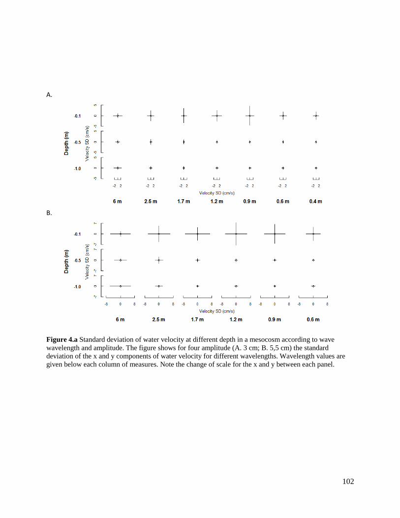
102

A.

B.

Figure 4.a Standard deviation of water velocity at different depth in a mesocosm according to wave

wavelength and amplitude. The figure shows for four amplitude (A. 3 cm; B. 5,5 cm) the standard

deviation of the x and y components of water velocity for different wavelengths. Wavelength values are

given below each column of measures. Note the change of scale for the x and y between each panel.

103

104

Comments and recommendations

The results of the tests of the prototype allowed us to conclude that the wave generator

and tank technical specifications could reproduce the water mixing in the wave column generated

by the surface waves. By comparison to theoretical specifications, the system is more flexible

and, for instance, it is possible to produce waves of 6.0 m wavelength with a small amplitude is

possible. Five additional mesocosms were installed in Spring 2012 and six more in Spring 2013.

Besides classical tanks of different volumes, the aquatic platform of the CEREEP Ecotron

IleDeFrance (Saint-Pierre-lès-Nemours, France) is equipped with 12 mesocosms with wave

generators.

A first experiment was conducted in Summer 2012 by Blottière et al (in prep) to test the

effects of mixing on water chemistry and the food-web dynamics of a freshwater community.

Two mixing regimes were compared and the experiment lasted nine weeks. The results show

effects of the treatment on water turbidity, phytoplankton and some zooplankton functional

groups and chemical parameters (Blottière et al. submitted). The results of this experiment suggest

that mixing affects the foodweb and chemical properties via a complex combination of direct

interaction through vertical displacement and indirect interaction through turbidity and sediment

resuspension.

Beyond the classical tank experiments focusing on the study of aquatic ecosystems,

though this experimental setup it is possible to also explores the different physical factors

structuring them. We give here four examples: 1) The nature and quantity of the sediments may

be manipulated as well as the timing of the surface waves. Our experimental setup allows one to

study the effects of shear stress at the sediment surface after different consolidation times.

(Kleeberg and Herzog 2014; Niemisto et al. 2008). 2) Light is the fuel of photosynthesis and light

105

absorption (see for instance Gallegos et al. 2008) determines light reflectance. Our experimental

setup can be used to the effects of surface water roughness due to waves, in interactions with the

concentration and quality of suspended matter and colored dissolved organic matter, on light

reflectance, a measure used for remote-sensing monitoring of lakes (Kutser et al. 2005; Yacobi et

al. 1995). 3) Contact surfaces of water with air and sediments are habitats for different species.

Benthic species, leaving in the sediments or at their surface, are better known than species using

water superficial tensions to stay afloat. (Suter 2013). 4) In addition, an artificial beach, with

different lengths and inclinations, can be put into the tank at the opposite side of the wave

generator. This set up could, for instance, reproduce in controlled experiments the beach or bank

erosion by waves (Liedermann et al. 2014; Lorang and Stanford 1993).

In conclusion, the mesocosm with a wave generator is a multipurpose tool to explore

surface and internal waves and the water motions they generate in the water column and at the

interfaces of water with air and sediments, respectively. This original experimental device opens

new opportunities for studying multiple interactions between ecological and physical processes in

ecosystems.

Acknowledgements

This project has succeeded thanks to the constant support of Régis Ferrière, Jean-François Le

Galliard and Gérard Lacroix. FDH appreciates greatly their encouragement; she is grateful to

Isabelle Jouanneau and Samuel Perret for their help during the prototype exploration. We thank

Jacques Gignoux and William XXX for comments and corrections on a previous draft.The

prototype and the additional mesocosms with generators were funded by XXX and the Projet

d‟Excellence Planaqua.

106

References

Becker, A., A. Herschel, and C. Wilhelm. 2006. Biological effects of incomplete destratification

of hypertrophic freshwater reservoir. Hydrobiologia 559: 85-100.

Blottière, L., M. Jaffar Bandjee, S. Jacquet, A. Millot, and F. D. Hulot. submitted. Effect of water

column mixing on freshwater ecosystems: a mesocosm experiment.

Blottière, L., M. Rossi, F. Madricardo, and F. D. Hulot. 2014. Modelling the role of phosphorus,

wind and warming on cyanobacterial (Microcystis aeruginosa) blooms in shallow lakes.

Theoretical Ecology 7: 35-52.

Burford, M. A., and M. J. O‟donohue. 2006. A comparison of phytoplankton community

assemblages in artificially and naturally mixed subtropical water reservoirs. Freshwater

Biology 51: 973–982.

Diehl, S., S. Berger, R. Ptacnik, and A. Wild. 2002. Phytoplankton, light, and nutrients in a

gradient of mixing depths: field experiments. Ecology 83: 399–411.

Gallegos, C. L., R. J. Davies-Colley, and M. Gall. 2008. Optical closure in lakes with contrasting

extremes of reflectance. Limnol. Oceanogr. 53: 2021-2034.

Gignoux, J., I. D. Davies, S. R. Flint, and J.-D. Zucker. 2011. The Ecosystem in Practice: Interest

and Problems of an Old Definition for Constructing Ecological Models. Ecosystems 14:

1039-1054.

Hawkins, P. R., and D. J. Griffiths. 1993. Artificial destratification of a small tropical reservoir:

effects upon the phytoplankton. Hydrobiologia 254: 169-181.

Hudnell, H. K., C. Jones, B. Labisi, V. Lucero, D. R. Hill, and J. Eilers. 2010. Freshwater

harmful algal bloom (FHAB) suppression with solar powered circulation (SPC). Harmful

Algae 9: 208-217.

107

Huisman, J., P. Van Oostveen, and F. J. Weissing. 1999a. Critical depth and critical turbulence:

Two different mechanisms for the development of phytoplankton blooms. Limnol

Oceanogr 44: 1781-1787.

---. 1999b. Species dynamics in phytoplankton blooms: Incomplete mixing and competition for

light. Am. Nat. 154: 46-68.

Hyun, J. M. 1976. Theory for hinged wavemakers of finite draft in water of constant depth. J.

Hydronautics 10: 2-7.

Kleeberg, A., and C. Herzog. 2014. Sediment microstructure and resuspension behavior depend

on each other. Biogeochemistry 119: 199-213

Kutser, T., D. Pierson, L. Tranvik, A. Reinart, S. Sobek, and K. Kallio. 2005. Using satellite

remote sensing to estimate the colored dissolved organic matter absorption coefficient in

lakes. Ecosystems 8: 709-720.

Liedermann, M. and others 2014. Typification of vessel-induced waves and their interaction with

different bank types, including management implications for river restoration projects.

Hydrobiologia 729: 17-31.

Lorang, M., and J. Stanford. 1993. Variability of shoreline erosion and accretion within a beach

compartment of Flathead Lake, Montana. Limnol. Oceanogr. 38: 1783-1795.

Niemisto, J., H. Holmroos, Z. Pekcan-Hekim, and J. Horppila. 2008. Interactions between

sediment resuspension and sediment quality decrease the TN : TP ratio in a shallow lake

Limnol. Oceanogr. 53: 2407-2415

Oberholster, P. J., A.-M. Botha, and T. E. Cloete. 2006. Toxic cyanobacterial blooms in a

shallow, artificially mixed urban lake in Colorado, USA. Lakes & Reservoirs: Research

and Management 11: 111-123.

108

Ogilvie, B. G., and S. F. Mitchell. 1998. Does sediment resuspension have persistent effects on

phytoplankton? Experimental studies in three shallow lakes. Freshwater Biology 40: 51-

63.

Read, J. S., A. Shade, C. H. Wu, A. Gorzalski, and K. D. Mcmahon. 2011. Gradual Entrainment

Lake Inverter” (GELI): A novel device for experimental lake mixing. Limnol. Oceanogr.:

Methods 9: 14-28.

Reynolds, C. S. 2006. The ecology of freshwater phytoplankton. Cambridge University Press.

Reynolds, C. S., S. W. Wiseman, B. M. Godfrey, and C. Butterwick. 1983. Some effects of

artificial mixing on the dynamics of phytoplankton populations in large limnetic

enclosures. Journal of Plankton Research 5: 203-234.

Scheffer, M. 1998. Ecology of shallow lakes. Chapman & Hall.

Steinberg, C. 1983. Effects of artificial destratification on the phytoplankton populations in a

small lake. Journal of Plankton Research 5: 855-864.

Suter, R. B. 2013. Spider locomotion on the water surface: biomechanics and diversity. Journal of

Arachnology 41: 93-101.

Thorpe, S. 2004. Langmuir circulation. Annu. Rev. Fluid Mech. 36: 55-79.

Upadhyay, S., K. A. Bierlein, J. C. Little, M. D. Burch, K. P. Elamc, and J. D. Brookesb. 2013.

Mixing potential of a surface-mounted solar-powered water mixer (SWM) for controlling

cyanobacterial blooms. Ecological Engineering 61: 245-250.

Visser, P., B. Ibelings, B. Vanderveer, J. Koedood, and L. Mur. 1996. Artificial mixing prevents

nuisance blooms of the cyanobacterium Microcystis in Lake Nieuwe Meer, the

Netherlands. Freshwater Biol 36: 435-450.

109

Weithoff, G., A. Lorke, and N. Walz. 2000. Effects of water-column mixing on bacteria,

phytoplankton, and rotifers under different levels of herbivory in a shallow eutrophic lake.

Oecologia 125: 91-100.

Wetzel, R. G. 2001. Limnology. Lake and River Ecosystems, 3rd ed. Academic Press.

Yacobi, Y., A. Gitelson, and M. Mayo. 1995. Remote-sensing of chlorophyll in Lake Kinneret

using spectral-resolution radiometer and landsat-TM - spectral features of reflectance abd

algorithm development. Journal of Plankton Research 17: 2155-2173.

110

111

Chapter III

112

113

How does water mixing affect the pelagic food-web in

shallow lakes?

Blottière L. Jaffar Bandjee M., Jacquet S., Millot A. and Hulot F.D.

In preparation for submission to limnology & Oceanography

Keywords: Shallow lake, mixing, phytoplankton, zooplankton, foodweb, mesocosms,

wave-makers, water chemistry, wind

114

Abstract

We examined the effects of wind-induced mixing and sediment resuspension on typical

food webs of temperate shallow lakes. These processes are known to have a major impact on the

phytoplankton community, light penetration, and nutrient availability in the water column.

However, little is known about the global effects of these processes on freshwater food webs. We

thus conducted a 9-week experiment comprising a manipulation of mixing intensity in 15 m3

mesocosms with wave-makers in order to explore the impact of two mixing intensities on water

chemistry as well as viral, bacterial, phytoplankton, and zooplankton communities. The turbidity

level in mixed mesocosms (compared to calm conditions) was higher on average, especially at

the bottom, indicating resuspension of the sediment bed. Mixing increased chlorophyll a

concentration without any clear increase in algal abundance, which pointed to a physiological

adaptation to mixing. A strong positive effect was also found on pH, suggesting an increased

primary productivity in well-mixed systems. Zooplankton responses to mixing were neutral for

cladocerans and rotifers, but negative for copepods. Finally, bacterial and viral abundances were

unchanged by the mixing regimes, but viral lysis of heterotrophic bacteria could be enhanced by

the water column mixing. Our experiment demonstrates that mixing is likely to influence shallow

lake functioning through a complex combination of direct and indirect effects on the underwater

light climate and water chemistry, phytoplankton physiology and productivity, zooplankton

growth, and possibly virus-host interactions. These complex effects could play a major role in

structuring pelagic and benthic communities in shallow lakes.

115

Introduction

Wind-induced mixing is a key process in shallow lakes (Reynolds et al. 1983, 1984;

Carrick et al. 1993; Schelske et al. 1995; Søndergaard et al. 2003; Reynolds 2006). In addition to

mixing the water column, wind forcing usually generates sufficient shear stress to cause the

erosion and resuspension of bottom material. As a result, vertical mixing can significantly affect

the underwater light climate, nutrient availability, and distribution of organisms (Wetzel 2001). In

nature, freshwater lakes experience different mixing regimes depending on the local climate, their

morphometry, thermal stratification, and exposure to wind. Indeed, this natural heterogeneity in

mixing regimes might have important consequences on the functioning and structure of such

ecosystems.

Wind-induced mixing has long been recognized as a major factor impacting phytoplankton

biomass, growth, and community composition. Phytoplankton species, whether motile, non-

motile, or buoyant, respond differently to water stability. Typically, microstratification within the

euphotic zone generally favors motile or buoyant species, while fast-sinking species like diatoms

or desmids are quickly lost from suspension (Reynolds et al. 1983; 2006). Sinking species rely

heavily on mixing processes to maintain or be resuspended in the photic zone. The seasonal

succession of phytoplankton groups in temperate lakes has been shown to be regulated in part by

shifts in mixing patterns and intensities (typically in autumn and spring) (Reynolds et al. 1983,

1984; Sommer et al. 2012). Further, the different strategies exhibited by phytoplankton with

regard to mixing intensity have been successfully studied through modelling (Huisman and

Weissing 1994; Huisman et al. 1999, 2004; Klausmeier and Litchman 2001; Blottière et al. 2013;

Aparicio Medrano et al. 2013) and used in water management to prevent bloom-forming

cyanobacteria in stratified lakes and reservoirs using artificial mixing (Hawkins and Griffiths

116

1993; Visser et al. 1996; Jungo et al. 2001; Burford and O‟Donohue 2006; Jöhnk et al. 2008;

Hudnell et al. 2010).

In shallow lakes, mixing has a direct influence on water quality as it affects turbidity levels

(Bengtsson and Hellström 1990; Luettich et al. 1990; Bengtsson and Hellstrom 1992). Indeed, by

resuspending matter from the sediment bed, mixing increases light attenuation, which can in turn

reduce algal growth and productivity. For instance, Hellström (1991) calculated a 85% reduction

in algal production following storm events in Lake Tämnaren (Sweden). However, most studies

with a simulation of resuspension events showed a short- and long-term increase (from a few

hours to a week) in chlorophyll concentrations, algal productivity, and growth, with no visible

adverse effect of turbidity (Ogilvie and Mitchell 1998). This positive outcome of mixing and

resuspension is mainly explained by the inoculation of meroplanktonic algae in resting stages into

the water column, thus changing community compositions and increasing phytoplankton biomass

and chlorophyll a concentration (Carrick et al. 1993; Schelske et al. 1995; Head et al. 1999;

Schallenberg and Burns 2004; Verspagen et al. 2004, 2005). Through the resuspension of

sediments, mixing also increases the possibility of releasing high quantities of nutrients and,

especially, phosphorus into the water (Søndergaard et al. 1992; Søndergaard et al. 2003; Zhu et

al. 2005; Reynolds 2006). Nutrient input from the sediment might alleviate nutrient limitation and

thus positively affect phytoplankton growth and biomass. In an attempt to disentangle the

influences of light, nutrients, and algal entrainment, Schallenberg and Burns (2004) reported that

meroplankton resuspension and, to a lesser extent, nutrient release were the main mechanisms

through which phytoplankton was impacted by mixing. Light limitation due to increased turbidity

was shown to be unlikely, except in very high turbidity levels that only coincide with extreme

weather events.

117

Despite the large number of studies on mixing in shallow lakes, little is known about the

overall impact of mixing on trophic levels other than phytoplankton. A few studies have

investigated the effects of mixing and resuspension on bacteria and the benthic microbial food

web, observing a global positive effect of resuspension on bacterial and protist growth (Weithoff

et al. 2000; Garstecki and Wickham 2001). Eckert and Walz (1998) explored the link between the

frequency of wind events and zooplankton succession in a shallow polymictic lake in Germany,

while Levine et al. (2005) studied how wind-induced resuspension decreased the feeding and

clearance rates of Daphnia and Boeckella hamate in Lake Waihola (New Zealand). Weithoff et

al. (2000) studied more than one trophic level by simultaneously testing the effect of two

consecutive resuspension events on three trophic bacteria, phytoplankton, and rotifers,

demonstrating a positive effect on bacteria and phytoplankton through enhanced nutrient

availability, which could in turn favor rotifers. Nevertheless, more studies are needed on multiple

trophic levels in order to better understand the global effects of mixing on the whole ecosystem.

In this study, we aim to present a general pattern to show whether and how water mixing

impacts the trophic food web through direct physical effects or indirect pathways. To explore this

phenomenon, we used a unique experimental set-up with mesocosms equipped with wave-makers

(Hulot et al. in prep.). The goal was to mimic as closely as possible the natural water motion

induced by continuous moderate winds in lakes. Previous attempts to study mixing were usually

conducted in situ using bubbling systems or manual mixing of the water column, which might not

be representative of natural wind-induced mixing (reviewed in Hulot et al. in prep.). We used

these mesocosms over 9 weeks to follow the physical, chemical, and biological responses of our

systems to two mixing levels: 1) complete mixing of the water column plus resuspension, which

118

mimics well-exposed shallow lakes; 2) superficial mixing of the top water layer and no

resuspension, which concerns unexposed shallow lakes.

Materials and methods

Study site and experimental design

The experiment was run from July to September 2012 at the CEREEP-Ecotron Ile-de-

France (Equipex Planaqua, St-Pierre-lès-Nemours, France). We used six rectangular mesocosms

(10 x 1.5 x 1.5 m) made of 10 cm insulating polyester covered with a liner. Each mesocosm has a

wave generator fixed at one extremity, with the mechanism described in detail in Hulot et al.

(submitted). In short, a paddle rotates around an axis assembled at its basis, while the paddle

oscillations generate surface stationary waves. The wavelength and amplitude of waves are

determined by the frequency and amplitude of paddle oscillations, respectively. All enclosures

were filled with tap water, reaching a final total volume of 15 m3 and a water column of 1 m. To

create a sediment bed, approximately 300 L of sieved sand from the Loire River (France) were

put into each mesocosm as homogeneously as possible. At the same time, we used four circular

containers of ~1.5 m3 to cultivate algae and zooplankton collected from natural communal lakes

and ponds nearby the experimental site. The diversity in these containers was maintained by

regularly adding water from the same lakes and ponds. They were used as reservoirs for

reseeding the mesocosms on a weekly basis throughout the experiments in order to limit the loss

of diversity due to species selection (Mette et al. 2011) and ensure the development of potential

populations in favorable environmental conditions (Hulot et al. 2014). On July 10, each

mesocosm was seeded with phytoplankton and then the following week with zooplankton.

Phosphorus was added along with phytoplankton using a K2HPO4 solution to reach a final

mesocosm concentration of 70 µg P. L-1

. Four days after zooplankton introduction, eight or nine

119

planktivorous cyprinid fish (Carassius carassius, purchased from SARL Vinal fishfarm, France)

were added to each mesocosm with a mean density of 9.10 ± 1.02 g m-3

.

To test the impact of mixing on shallow lakes, the experimental design had two treatment

levels (“mixed” and “calm”) run in triplicates. In three of the mesocosms, we generated long

wavelength waves (about 3.5 m) to mix the entire water column and create friction forces at the

sediment surface so as to ensure the regular resuspension of the bottom-top layer and sedimented

particles (“mixed” treatment). In the other three mesocosms, short wavelength waves were

generated to create a very superficial mixing (“calm” treatment). The machines were activated

immediately after the fish addition on July 20.

Physical measurements and water chemistry

All mesocosms were sampled weekly (July 23: date 0 to September 19: date 9), and all

measurements were taken at two different depths: below the surface and just above the sediment

bed. Samples and measurements were taken at the center of the enclosures from a small ramp

fixed on top of each mesocosm. Mesocosms were sampled in random order on each occasion.

Physical parameters such as temperature, pH, oxygen concentration, conductivity, and

nephelometric turbidity (expressed in NTU) were measured directly in the mesocosms using a

multiparameter probe (YSI 6600 V2-4-M).

Water samples for total suspended solids (TSS), dissolved nutrient concentrations,

phytoplankton, zooplankton, and flow cytometry analyses were taken with a 2.2-l Alpha model

Van Dorn horizontal water sampler (Anhydre). TSS (in dry weight per liter) were obtained by

filtering a known water volume (typically 1 L, more or less depending on the particulate density)

through pre-weighted and dried 0.7 µm pore size Whatman GF/F filters and then weighting the

120

filters again after at least 24 hours of drying in an oven at 105 °C. The filtered water was then

used in the laboratory to measure dissolved nutrient concentrations with a spectrophotometer

(DR3900 Hach Lange). Orthophosphates were determined using the vanadate-molybdate method

(LCK349 Kit Hach Lange). Total nitrogen was determined using the Koroleff digestion

(Peroxodisulphate) and photometric detection with 2.6-Dimethylphenol (LCK138 Hach Lange

Kit). Nitrate, ammonium, and nitrite were respectively determined using the cadmium reduction,

diazotation, and salycilate methods (Hach Lange kits: Nitraver 5, Nitriver 3, and Ammonia

Nitrogen reagent set).

Phytoplankton and zooplankton

Phytoplankton samples were divided into three size classes directly on site using

differential filtration, i.e., a consecutive filtration through 100 µm and 30 µm mesh-size nylon

filters. Hence, we had three subsamples: unfiltered water with algae of all sizes, a subsample with

algae below 100 µm in the greatest axial linear dimension (GALD), and a subsample with algae

below 30 µm in GALD. These subsamples were kept in the dark for 15 min before taking

fluorescence measurements using the BBE FluoroProbeTM

spectrofluorometer (Moldaenke) in

laboratory. This fluoroprobe provides an estimate of chlorophyll a content (expressed in

equivalent µg L-1

of Chl-a) by measuring in vivo autofluorescence of pigment-containing micro-

organisms (Beutler et al. 2002, Leboulanger et al. 2002, Rolland et al. 2010). The probe allows us

to differentiate four phytoplankton groups referred to as “green” (chlorophyta and Euglenophyta),

“brown” (Bacillariophyta, Chrysophyta, and Euglenophyta), “blue” (Cyanophyta), and “red”

algae (Cryptophyta). Preliminary results showed that there were no algae larger than 100 µm,

therefore the biomass of algae between 30 and 100 µm in GALD was obtained by subtracting the

biomass values of algae under 30 µm from the 100 µm filtered sample value.

121

Three to five liters were filtered through 30 µm mesh-size nylon filters to collect

zooplankton, which were immediately fixed in a solution of 96% ethanol and 4% glycerol (72%

and 1% final concentration, respectively) to avoid body deformation. Samples were then

exhaustively identified to the genus or species level and counted under a microscope.

For flow cytometry (FCM) analysis of small phytoplankton, prokaryote, and virus

abundance, 4 mL of water was filtered through 30 µm mesh-size nylon filters and immediately

fixed with paraformaldehyde (1% final concentration). The samples were then plunged into liquid

nitrogen for 1 min before storage at -80 °C. Just before FCM analysis, samples were thawed at

room temperature for a few minutes. Autotrophic small eukaryotes, picocyanobacteria,

heterotrophic bacteria, and virus-like particles (VLPs) were counted using a FACSCalibur flow

cytometer (Becton Dickinson) equipped with an air cooled laser providing 15 mW at 488 nm. For

the analysis of VLPs and bacteria, samples were diluted in 0.02 µm filtered TE buffer (0.1 mM

Tris–HCL and 1 mM EDTA, pH 8), and incubated with SYBR Green I (at a final 10-4

dilution of

the commercial stock solution; Molecular Probes) for 5 min at ambient temperature, followed by

10 min heating at 75°C and then another 5 min at room temperature, prior to FCM analysis

(based on Brussaard 2004 and modified by Jacquet et al. 2013.). For photosynthetic cells (i.e.,

picocyanobacteria and small eukaryotes), no fluorochrome was used; analysis was thus made on

fixed samples to which we added a suspension of 1-µm beads (molecular probes). The flow

cytometer list mode files thus obtained were then transferred and analyzed on a PC using the

custom-designed software CYTOWIN (Vaulot 1989).

Statistical analysis

Statistical analyses were performed using the R software version 3.0.3 (www.r-

project.org).The data set from the first date was analyzed using the Wilcoxon test in order to test

122

the homogeneity between mesocosms. To test the effects of mixing on the biological and

chemical variables measured, we constructed linear mixed-effects models (LME, fit by REML -

nlme packages -, Pinheiro et al. 2013, R Core Team. 2014) with time, treatment, and their

interaction as fixed effects. Individual mesocosms were treated as a random effect. Furthermore,

heteroscedasticity correction and auto-correlation structures using AR(1) function (Pinheiro and

Bates 2000) were added to the models when the homogeneity and independence hypothesis were

violated. Residuals were visually checked to assess the quality of the model. The effects of depth

were tested on every variable, and when non-significant, further statistical analyses were

conducted on the mean values between depths (every variable except for turbidity and TSS).

Prior to these analyses, the normality and homoscedasticity of each variable were assessed

visually, and log or sqrt corrections were applied when necessary.

Results

Initial conditions

At the start of the experiment (date 0), dissolved phosphorus and nitrogen concentrations

were 0.017±0.005 mg L-1

and 5.855±0.097 mg L-1

, respectively. Total chlorophyll a

concentration was 24.60±4.00 µg L-1

with a large dominance of green algae compared to

cyanobacteria and diatoms (21.61±3.80, 2.63±1.84, and 0.35±0.24 µg Chl a L-1

, respectively).

Phytoplankton abundance assessed using FCM was 1.01x106

±4.12 x104

and 1.08x106

± 4.10

x104

cells mL-1

in mixed and calm mesocosms, respectively. Prokaryote (essentially heterotrophic

bacteria) as well as virus-like particle abundance were also very similar between mixed and calm

treatments (prokaryotes: 4.6x106

±3.2 x106 vs. 4.3x10

6 ±5.8 x10

5 cells mL

-1; virus: 6.5 x10

6±2.0

x105 vs. 6.1 x10

6±5.3 x10

5 part mL

-1). Zooplankton was largely dominated by rotifers on the first

date with 63±13 individuals L-1

. Crustacean concentration was very low at the beginning with

123

only a few Bosmina longirostris, Scapholebris mucronata, and calanoids. Between-treatment

comparison on the first date for all physical, chemical, and biological variables showed no

significant differences (Wilcoxon test, P>0.05).

Water mixing effects on turbidity and water chemistry

Mixing increased the nephelometric turbidity in the more turbulent mesocosms, while it

decreased slightly in calm conditions (Fig.1a, Table 1, LME, Mixing x Time: F1,99=13.556,

p=0.0004). Surface turbidity of mixed mesocosms was similar to the turbidity level at the bottom

of the calm mesocosms (Fig.1a). Overall, the nephelometric turbidity was always greater at the

bottom compared to the surface, except during the first week of the experiment (LME, Depth:

F1,99=77.863, p<0.0001). On average, the turbidity was maximal at the bottom of mixed

mesocosms with a mean value of 14.8±2.2 NTU, suggesting the continuous resuspension of the

sediment top layer.

TSS had similar dynamics. TSS concentration increased in the mixed mesocosms from the

4th

week until the end of the experiment, while it remained stable under calm conditions (Fig.1b,

Table 1). TSS concentrations at the end were 14.6±5.4 mg L-1

and 8.0±0.9 mg L-1

in mixed and

calm mesocosms, respectively. TSS concentration was strongly correlated to green algae biomass

(spearman rank correlation, rho=0.677, p=<0.0001), suggesting that most of the suspended solids

in our mesocosms were phytoplankton cells and cell debris.

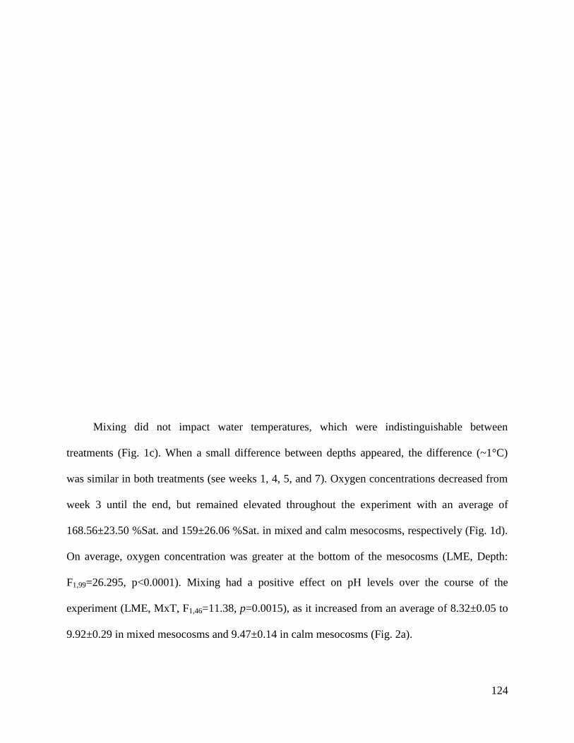
124

Mixing did not impact water temperatures, which were indistinguishable between

treatments (Fig. 1c). When a small difference between depths appeared, the difference (~1°C)

was similar in both treatments (see weeks 1, 4, 5, and 7). Oxygen concentrations decreased from

week 3 until the end, but remained elevated throughout the experiment with an average of

168.56±23.50 %Sat. and 159±26.06 %Sat. in mixed and calm mesocosms, respectively (Fig. 1d).

On average, oxygen concentration was greater at the bottom of the mesocosms (LME, Depth:

F1,99=26.295, p<0.0001). Mixing had a positive effect on pH levels over the course of the

experiment (LME, MxT, F1,46=11.38, p=0.0015), as it increased from an average of 8.32±0.05 to

9.92±0.29 in mixed mesocosms and 9.47±0.14 in calm mesocosms (Fig. 2a).

125

Table 1. Results of the mesocosm experiment carried out in summer 2012.

P-values

Response variables Mixing (M) Time (T) M x T Depth

Turbidity

Nephelometric turbidity (NTU) 0.0207 n.s. 0.0004 <0.0001

TSS (mg L-1

) 0.0113 0.0377 0.0363 0.0478

Chemistry

Oxygen (%Sat.) n.s. <0.0001 n.s. <0.0001

pH 0.0129 <0.0001 0.0015

NO3-N (mg L-1

) n.s <0.0001 n.s.

NO2-N (mg L-1

) 0.0886* <0.0001 <0.0062

NH3-N (mg L-1

) n.s 0.0248 n.s.

PO43-

(mg L-1

) n.s n.s. n.s

Phytoplankton

Green algae (µg Chl a L-1

) 0.0434 0.0001 0.0008

GALD<30 µm (µg Chl a L-1

) n.s. 0.0132 0.0024

30<GALD<100 µm (µg Chl a L-1

) 0.0483 <0.0001 <0.0001

Abundance (cell mL-1

) n.s. 0.0093 n.s.

Virus and bacteria

Virus (VLP mL-1

) n.s. 0.0024 n.s.

Bacteria (cell mL-1

) n.s. n.s. n.s.

Zooplankton

Zooplankton (ind. L-1

) n.s. <0.0001 n.s.

Rotifer (ind. L-1

) n.s. <0.0001 n.s.

Bosmina (ind. L-1

) n.s. <0.0001 n.s.

Nauplii (ind. L-1

) n.s <0.0001 n.s.

Copepode (ind. L-1

) 0.0644* <0.0001 0.0003

n.s = not significant, * marginally significant.

126

The concentration of dissolved nitrates, ammonium, and phosphates and their temporal

dynamics were similar in mixed and calm mesocosms (Fig. 2b, c, d, Table 1). Nitrate

concentration decreased over time from 3.57±0.41 mg L-1

to 2.21±0.21 mg L-1

in all mesocosms,

suggesting assimilation by the phytoplankton. Nitrite temporal dynamic differed significantly

between treatments (Fig. 2e), with a greater accumulation of nitrites in calm mesocosms (LME,

MxT, F1,46=8.23, p<0.0001).

127

Water mixing effects on phytoplankton

The most abundant phytoplankton species found in the mesocosms throughout the

experiment were the three chlorophycae, Coelastrum sp., Pediastrum sp., and Ankistrodesmus sp.

According to the BBE fluoroprobe, more than 80% of chlorophyll a content was attributable to

the “green” algal group in all mesocosms (Fig. 3). As a result, we will mainly focus on green

algae.

In both treatments, we observed an increase in chlorophyll a content for the first three

weeks of the experiment (Fig. 4a). Chlorophyll a concentration subsequently decreased and

stabilized in calm conditions, while it continued to increase in mixed mesocosms (LME, MxT, F1,

46=12.872, p=0.0008). At the end of the experiment, “green algae” chlorophyll a content reached

102.01±31.11 µg Chl a L-1

in mixed mesocosms compared to 41.54±17.71 µg Chl a L-1

in calm

conditions. This positive response to mixing was found for both “small” and “large” green algae

(Fig. 4b, 4c). Overall, 60% of the total chlorophyll a concentration was found in “small” green

Figure 3. Proportion of phytoplankton classes during the 9 weeks experiment. “M” and “C” are

respectively mixed and calm mesocosms. Green algae are in light grey, diatoms in light grey and

bluegreen algae in black.

128

algae (less than 30 µm in GALD) (Fig. 4b). Larger algae (between 30 µm and 100 µm, Fig. 4c)

reached higher chlorophyll a content in mixed mesocosms (last week of the experiment:

34.18±11.90 vs 12.37±2.58 µg Chl a L-1

).

129

FCM data on phytoplankton indicated an increase in abundance (in cells mL-1

) during the

first three weeks of the experiment in accordance with chlorophyll a measurements (Fig. 4d).

However, while we observed a between-treatment divergence in chlorophyll a concentration

using the BBE probe, here we found a steady decline in cell abundance until the end of the

experiment in both treatments.

Water mixing effects on zooplankton

The zooplankton communities in this experiment were found to be typical of a high

predation rate by planktivorous fishes, i.e., the dominant species were small, mainly comprising

herbivorous rotifers and the cladoceran Bosmina longirostris (Fig. 5a, b, c, and d). Rotifers

formed more than 90% of zooplankton abundance at all times. Rotifer community composition

changed over time, but it was dominated by planktonic genera such as Keratella cochlearis,

Anueropsis fissa, Polyarthra sp., and Brachionus sp. Other small cladocerans like Scapholebris

sp., Ceriodaphnia sp., and Diaphanosoma brachyurum also appeared during the experiment,

albeit rarely. Nauplii and copepodes (calanids and cyclopids) were mainly found from the second

half of the experiment onwards.

Rotifer abundance increased up to ~2200 individuals per liter in both treatments. The

abundance peak was reached at week 6 in calm mesocosms and week 8 in mixed mesocosms

(Fig. 5b). In calm conditions, we then observed a steady decline until the end of the experiment.

Despite this difference in dynamic, no statistical effect of mixing was found for rotifer

abundance. Bosmina longirostris abundance and dynamic was very similar in both treatments

over time, with increasing abundance in the second half of the experiment (Fig. 5c). Mixing

intensity only had a significant effect on copepods over time (LME, MxT: F1,46=15.415,

130

p=0.0003), reaching higher densities in clam mesocosms (Fig. 5d). This result was not found for

copepod larvae, i.e., nauplii, even though the graphical patterns are similar (Fig. 5e).

131

Water mixing effects on prokaryotes and virus-like particles

Temporal dynamics of virus-like particles and prokaryotes were globally indistinguishable

between the mixing treatments (Fig. 4e, f). Virus abundance increased during the first 4 weeks,

while prokaryote abundance decreased. Inversely, the prokaryote abundance suddenly increased

in weeks 5 and 6, while virus abundance dropped. In calm conditions, the virus-to-prokaryote

ratio (VPR) remained relatively low and homogenous between mesocosm replicates. Conversely,

in mixed conditions, each replicate displayed a relatively high VPR value at different moments of

the experiment (Fig. 6: weeks 3, 4, and 7 for mesocosms 3, 5, and 1, respectively).

Figure 6. Temporal dynamics of the VRP ratio in each mesocosms. Black line: mixed mesocosms, grey line:

calm mesocosms. Each mesocosm (from 1 to 6) is identified by a specific dot shape.

132

Discussion

To the best of our knowledge, this is the first experiment to investigate the effects of water

mixing and resuspension on shallow ecosystems using a new, efficient, and more appropriate

artificial wave-maker tool than previously proposed in the literature. In our experiment, we

successfully created two distinct environments: 1) a well-mixed and turbulent water column with

the resuspension of bottom materials leading to higher turbidity; 2) a stable water column with

only superficial mixing (comparable to calm conditions) and no resuspension. In fine, we found

two different types of food web functioning that we will discuss below.

Mixing effects on turbidity and sediments

As expected, turbidity and TSS concentration were greater in mixed mesocosms, with

maximum values at the bottom indicating the resuspension of the top layer of the sediment bed.

However, the impact on overall turbidity was moderate, with values never exceeding 20 NTU in

mixed mesocosms. Turbidity levels in lakes are of great importance for primary production, as it

reduces light availability for phytoplankton and macrophytes. The effect of resuspension on

phytoplankton production depends on the amount of matter that is resuspended for a given

mixing intensity (which depends on the sediment composition and cohesion) and on the threshold

of phytoplankton species for light limitation. Schallenberg and Burns (2004) showed that the

threshold for light limitation of phytoplankton was rather high, e.g., >200 NTU. These levels of

turbidity are most likely to be seen after strong weather events like storms. It is therefore unlikely

that algae would suffer from strong light limitation with the moderate level of continuous mixing

as seen in our experiment.

133

Mixing effects on nutrient concentration

In eutrophic shallow lakes, wind-induced resuspension is usually associated with the

release of total phosphorus from the sediments (Sondergaard et al. 1992; Hamilton and Mitchell

1997; Zhu et al. 2005; Thomas and Schallenberg 2008). Visible effects on dissolved phosphorus

are less common, as dissolved nutrients are subject to rapid biological assimilation and depend on

the difference in concentration between sediment-bound and dissolved phosphorus in the water

(Gunatilaka 1982; Hamilton and Mitchell 1997; Schallenberg and Burns 2004). In this

experiment, we did not observe any significant differences in dissolved phosphorus

concentrations between the mixed and unmixed enclosures. This can partly be explained by the

nature of the sediments chosen in our experiment, that is, sieved sand from the Loire River

(France). Even though we did not measure nutrient concentrations in the sand prior to the

experiment, it is rather safe to suggest that phosphorus concentration was very low compared to a

fresh sediment layer from a eutrophic shallow lake. Phosphorus release following mixing events

has been shown to have a positive impact on phytoplankton (Schallenberg and Burns 2004; Zhu

et al. 2005) and bacterial biomass (Weithoff et al. 2000). Indeed, this positive effect will only be

found when phytoplankton and procaryotes are in a state of nutrient limitation (Schallenberg and

Burns 2004).

No difference was observed in nitrogen concentration and dynamics except for nitrite

nitrogen. NO2 increased in both mixed and calm mesocosms, which usually indicates a

dysfunctioning of the nitrogen cycle. Nitrite accumulation often occurs in anoxic waters, which

was not the case in this experiment where oxygen levels in the water column were elevated

throughout the experiment. However, it is known that Nitrobacter, the primary bacterial genus

involved in the oxidation of nitrites to nitrates, is less tolerant of high pH values (Wetzel 2001).

134

In both treatments, pH levels were rather high, which could explain this trend. Further, NO2

accumulation was greater in calm as opposed to more turbulent conditions. The lack of

oxygenation of the sediment in unmixed mesocosms could reduce the nitrification activity in this

compartment (Chen et al. 1972). Similar results were found in the resuspension experiment of

Kang et al. (2013), where nitrites accumulated in mesocosms without resuspension, an effect that

was less pronounced when mixing was applied.

Mixing effects on phytoplankton and chlorophyll a concentrations

Higher concentrations of chlorophyll a were found in the mixed mesocosms. A positive

relationship between mixing and chlorophyll a has been found in numerous studies (Carrick et al.

1993; Schelske et al. 1995; Hamilton and Mitchell 1997; Ogilvie and Mitchell 1998;

Schallenberg and Burns 2004). For example, Schelske et al. (1995) showed that chlorophyll a

concentrations exceeding 100 µg/L were highly correlated with wind speed in Lake Apopka

(Florida, USA). In all cases, however, an increase in algae abundance through the recruitment of

meroplanktonic algae was the leading cause of change in chlorophyll a concentration. In contrast,

we found no increase in the abundance of small algae (<30 µm in diameter) in our mesocosms.

This discrepancy between chlorophyll a measurements and abundance data suggests that the

increase in chlorophyll a was not due to the entrainment of sedimented or meroplanktonic algae.

This was more likely a physiological response of algae cells to mixing, leading to higher

chlorophyll a content (a hypothesis that was indeed corroborated by FCM fluorescence data, not

shown). Photosynthetic organisms have the capacity to regulate the amount of pigments in

response to the light climate and nutrient concentration (Falkowski 1984; Shin et al. 1987;

Longhurst and Glen Harrison 1989; Ibelings et al. 1994; Felip and Catalan 2000). An increase in

chlorophyll a content is usually a response to a more turbid environment, known as shade

135

adaptation. Therefore, the higher global turbidity level observed in our mixed mesocosms could

have induced an increase in chlorophyll a cell content. Another hypothesis to explain the

discrepancy between abundance data and chlorophyll a might be a shift in community toward

species with higher chlorophyll a cell content (Visser et al. 1996; Felip and Catalan 2000). Large

algae (30 µm<GALD<100 µm) also respond positively to mixing in terms of chlorophyll content.

In addition to the physiological adaptation described for smaller algae, large algae abundance

could also be enhanced through a reduction of loss rate by sedimentation.

Mixing effects on pH and primary productivity

Although not measured directly, we observed a greater photosynthetic activity in mixed as

opposed to calm mesocosms, as shown by the higher pH values. In summer, pH usually increases

in natural environments as a consequence of the uptake of inorganic carbon by the primary

producers for their photosynthetic activity (Schelske et al. 1974; Scheffer 1998; Reynolds 2006;

Moss 2010; Kosten et al. 2011). Previous studies on the effects of fluctuating light due to mixing

showed diverse physiological responses, often leading to an increase in photosynthetic rates (see

references in Litchman 2000). Early experiments evaluating the phytoplankton photosynthetic

response to vertical movement in oceans showed an enhancement of photosynthesis for

phytoplankton grown at fluctuating depths compared to the same phytoplankton species

maintained at a fixed depth (Marra 1978). The reduction in photoinhibition experienced in clear

waters and/or the reduction in light limitation in turbid environments are two mechanisms

proposed to explain this positive effect of mixing on primary production (Mallin and Paerl 1992).

On the one hand, regular mixing allows phytoplankton cells to be exposed to sufficient light by

increasing their probability of passing through the well-exposed surface layer. On the other hand,

136

it also decreases the risk of photoinhibition by moving phytoplankton cells rapidly through the

water column to less exposed depth.

Mixing effects on zooplankton dynamics

Zooplankton responses to mixing varied from one group to another. Small cladoceran,

mainly Bosmina longirostris, and rotifer abundances were consistent in calm and mixed

mesocosms. Nonetheless, rotifers dynamics slightly differed with an abundance peak in week 6 in

calm mesocosms followed by a steady decline, while rotifer abundance increased until week 8 in

mixed mesocosms. This difference in timing might be explained by copepod density, which was

higher in calm mesocosms during the second half of the experiment. Most copepod species in

their adult stages are very efficient predators, with rotifers often being their preferred prey. It has

been demonstrated that their feeding rate on rotifers is high enough to produce top-down control

(Brandl 2005). As to why copepod densities are significantly higher in calm mesocosms, we

propose three non-exclusive hypotheses that might explain these results. First, the turbulent flows

caused by mixing could hinder the kinematics of copepods. It might therefore be more difficult

and energy-consuming for individuals to maintain their position in the water (Yen et al. 2008),

leading to reduced feeding and growth rates. Second, copepods in mixed enclosures could

proportionally absorb more resuspended material that is lower in nutrient content as compared to

in low turbidity environments, thus reducing the efficiency of food assimilation (Gasparini et al.

1999). Copepods could also expend more energy sorting food from sediment, although according

to Levine et al. (2005), NTU levels around 15 NTU as in our mixed mesocosms only reduce

clearance rates by 3-8%. Kang (2012) also showed non-statistical differences in the ingestion

rates of food particles by a marine copepod at suspended sediment concentration of 10 mg L-1

.

Third, it is possible that suspended sediments could interfere with the mechanical or chemical

137

signals from both copepod preys (Levine et al. 2005) and their predators. This could in turn lower

their feeding success, growth rates, and reproduction rates (Paffenhöfer 1972; Oviatt 1981;

Turner and Tester 1989; Gasparini et al. 1999; Kang 2012).

Mixing effects on prokaryotes and viruses

Bacteria are a crucial component in limnetic food webs, yet very little is known about the

impacts of mixing on this specific group in lakes. Weithoff et al. (2000) showed that bacterial

abundance increases strongly after mixing events due to the nutrient input in the water column. In

our experiment, we did not observe any differences in abundance between mixed and calm

enclosures, which is not surprising considering that we did not observe any changes in nutrient

content.

In the last decades, viruses have been recognized as an important component in the

microbial food web. They have an especially strong impact on bacterial mortality and diversity

(Wommack and Colwell 2000; Weinbauer 2004). Our results on the VRP ratio (generally

considered as a proxy of the interactions between viruses and hosts, e.g., Parikka et al. in

revision) could suggest that the lysis activity was stronger in mixed compared to calm conditions.

We hypothesize that this result could reflect enhanced contact rates in mixed conditions. A

similar effect of water motion was proposed by Hudnell et al. (2010) regarding the control of

cyanobacteria by cyanophages. Further studies would be necessary to confirm our finding, which

could have important consequences on ecosystem microbial functioning.

Ecosystem level

This medium-term experiment reveals that water mixing may have multiple impacts on

shallow water bodies, either directly through mechanic action or turbidity levels or indirectly

138

Figure 7. Synthetic schema of the effects of mixing based on our experimental results. The different types

of arrow represent 6 interactions that structure the environment.

through the food web. In Figure 7, inspired by the framework proposed by Olff et al. (2009), we

have illustrated the effects of mixing based on our experimental results and the hypothetical

mechanisms behind them. Our results show how mixing changes the conditions of the water

column through either direct physical effects (e.g., sediment resuspension, copepod kinetics,

virus and prokaryote interactions, green algae chlorophyll a content and productivity) or indirect

effects (e.g., increasing green algae productivity, which in turn causes the pH to rise, or

resuspension of sediments, leading to a more turbid environment for algae and possibly impairing

copepod feeding activity).

Heterotrophic

bacteria Viruses

+

+

External forcing:

N-NO3 N-NH

3 NO

2 PO

4

3−

Sediments

Physical-mechanical interactions:

Small algae (Chl a) Large algae (Chl a)

Fish

Rotifers Bosmina

Copepodes

Mesocosm

Consumer-resource interactions:

Mixing intensity

Interactions between organisms and

conditions:

Turbidity pH

Chemical interactions:

+

+

+

+

-

+

+ +

-

- -

Host-parasite interactions:

139

In our experiment, mixing changed ecosystem functioning by enhancing the primary

productivity. Yet it also changed the structure of the community by differently affecting the

zooplankton community and possibly strengthening the viral impact on the prokaryotes. This

could have an important impact on energy pathways from lower to upper trophic levels. Mixing

and resuspension events are common features in shallow lakes that demand a broader analysis on

multiple trophic levels to fully comprehend their action on the ecosystem functioning. The

inclusion of abiotic factors and different types of interactions, albeit challenging, gives a better

understanding of how the food web behaves and adjusts to different environmental conditions.

Acknowledgements

We wish to thank François Rocher and Jean-Jacques Lamandé of the CEREEP Ecotron

station for their technical help regarding the repairs, maintenance, and setting up of the ramps on

the enclosures. We would also like to thank the CNRS station for their help and technical

support. L.B. and this work are financially supported by the ANR Pulse 2010 CEPL 01004 and

ANR Equipex PLANAQUA (ANR-10-EQPX-13-01) coordinated by the CEREEP-Ecotron

IleDeFrance (UMS 3194).

References

Aparicio Medrano, E., R. E. Uittenbogaard, L. M. Dionisio Pires, B. J. H. van de Wiel, and H. J.

H. Clercx. 2013. Coupling hydrodynamics and buoyancy regulation in Microcystis

aeruginosa for its vertical distribution in lakes. Ecol. Modell. 248: 41–56.

Bengtsson, L., and T. Hellstrom. 1992. Wind-induced resuspension in a small shallow lake.

Hydrobiologia 241: 163–172.

Bengtsson, L., and T. Hellström. 1990. Redistribution of sediments in three Swedish lakes.

Hydrobiologia 192: 167–181.

140

Beutler, M., K.H.Wilshire, B. Meyer, C. Moldaenke, C. Lüring, M. Meyerhöfer, H.P Hansen and

H. Dau.2002. A fluorometric method for the differentiation of algal populations in vivo and

in situ. Photosynth. Res. 72: 39–53.

Blottière, L., M. Rossi, F. Madricardo, and F. D. Hulot. 2013. Modeling the role of wind and

warming on Microcystis aeruginosa blooms in shallow lakes with different trophic status.

Theor. Ecol. 7: 35–52.

Brandl, Z. 2005. Freshwater copepods and rotifers: predators and their prey. Hydrobiologia 546:

457–489.

Brussaard, C. P. D. 2004. Optimization of procedures for counting viruses by flow cytometry.

Appl. Environ. Microbiol. 70: 1506–1513.

Burford, M. A., and M. J. O‟Donohue. 2006. A comparison of phytoplankton community

assemblages in artificially and naturally mixed subtropical water reservoirs. Freshwater

Biol. 51: 973–982.

Carrick, H. J., F. J. Aldridge, and C. L. Schelske. 1993. Wind influences phytoplankton biomass

and composition in a shallow, productive lake. Limnol. Oceanogr. 38: 1179–1192.

Eckert, B., and N. Walz. 1998. Zooplankton succession and thermal stratification in the

polymictic shallow Müggelsee ( Berlin , Germany ): a case for the intermediate disturbance

hypothesis ? Hydrobiologia 387-388: 199–206.

Falkowski, P. G. 1984. Physiological responses of phytoplankton to natural light regimes. J.

Plankt. Resarch 6: 295–307.

Felip, M., and C. Catalan. 2000. The relationship between phytoplankton biovolume and

chlorophyll in a deep oligotrophic lake: decoupling in their spatial and temporal maxima. J.

Plankt. Res. 22: 91–105.

Garstecki, T., and S. Wickham. 2001. Effects of resuspension and mixing on population

dynamics and trophic interactions in a model benthic microbial food web. Aquat. Microb.

Ecol. 25: 281–292.

Gasparini, S., J. Castel, and X. Irigoien. 1999. Impact of suspended particulate matter on egg

production of the estuarine copepod, Eurytemora affinis. J. Mar. Syst. 22: 195–205.

Gunatilaka, A. 1982. Phosphate adsorption kinetics of resuspended sediments in a shallow lake,

Neusiedlersee, Austria. Hydrobiologia 91-92: 293–298.

Hamilton, D. P., and S. F. Mitchell. 1997. Wave-induced shear stresses, plant nutrients and

chlorophyll in seven shallow lakes. Freshwater Biol. 38: 159–168.

141

Hawkins, P. R., and D. J. Griffiths. 1993. Artificial destratification of a small tropical reservoir:

effects upon the phytoplankton. Hydrobiologia 254: 169–181.

Head, R. M., R. I. Jones, and a. E. Bailey-Watts. 1999. An assessment of the influence of

recruitment from the sediment on the development of planktonic populations of

cyanobacteria in a temperate mesotrophic lake. Freshwater Biol. 41: 759–769.

Hellström, T. 1991. The effect of resuspension on algal production in a shallow lake.

Hydrobiologia 213: 183–190.

Hudnell, H. K., C. Jones, B. Labisi, V. Lucero, D. R. Hill, and J. Eilers. 2010. Freshwater

harmful algal bloom (FHAB) suppression with solar powered circulation (SPC). Harmful

Algae 9: 208–217.

Huisman, J., P. van Oostveen, and F. J. Weissing. 1999. Species Dynamics in Phytoplankton

Blooms: Incomplete Mixing and Competition for Light. Am. Nat. 154: 46–68.

Huisman, J., J. Sharples, J. M. Stroom, P. M. Visser, W. E. a. Kardinaal, J. M. H. Verspagen, and

B. Sommeijer. 2004. Changes in Turbulent Mixing Shift Competition for Light Between

Phytoplankton Species. Ecology 85: 2960–2970.

Huisman, J., and F. J. Weissing. 1994. Light-Limited Growth and Competition for Light in Well-

Mixed Aquatic Environments: An Elementary Model. Ecology 75: 507–520.

Hulot, F. D., G. Lacroix, and M. Loreau. 2014. Differential responses of size-based functional

groups to bottom-up and top-down perturbations in pelagic food webs: a meta-analysis.

Oikos 000:001-010.

Ibelings, B. W., B. M. a. Kroon, and L. R. Mur. 1994. Mixing in Lakes Acclimation to high of

photosystem a in a green cyanobacterium and and flux eukaryotic simulating alga

fluctuating densities , photosynthetic light in photon regimes induced mixing lakes. New

Phytol. 128: 407–424.

Jacquet, S., Dorigo U., Personnic S. (2013) A Few Tests Prior to Flow Cytometry and

Epifluorescence analysis of freshwater samples. In Stefanos Papandreou (Ed) Flow

Cytometry: Principles, Methodology and Applications, Chapter 1, Related Nova

publication, Nova Publishers Inc., New York, 1–30.

Jöhnk, K. D., J. Huisman, J. Sharples, B. Sommeijer, P. M. Visser, and J. M. Stroom. 2008.

Summer heatwaves promote blooms of harmful cyanobacteria. Glob. Chang. Biol. 14: 495–

512.

Jungo, E., P. M. Visser, J. Stroom, and L. R. Mur. 2001. Artificial mixing to reduce growth of the

blue-green alga Microcystis in Lake Nieuwe Meer , Amsterdam : an evaluation of 7 years

of experience. Water Sci. Technol. Water Supply 1: 17–23.

142

Kang, H. K. 2012. Effects of suspended sediments on reproductive responses of Paracalanus sp.

(Copepoda: Calanoida) in the laboratory. J. Plankton Res. 34: 626–635.

Kang, Y., X. Song, and Z. Liu. 2013. Sediment resuspension dampens the effect of nutrient

inputs on the phytoplankton community: A mesocosm experiment study. Hydrobiologia

710: 117–127.

Klausmeier, C. a., and E. Litchman. 2001. Algal games: The vertical distribution of

phytoplankton in poorly mixed water columns. Limnol. Oceanogr. 46: 1998–2007.

Kosten, S., V. L. M. Huszar, E. Bécares, L. S. Costa, E. Donk, L.-A. Hansson, E. Jeppesen, C.

Kruk, G. Lacerot, N. Mazzeo, L. Meester, B. Moss, M. Lürling, T. Nõges, S. Romo, and M.

Scheffer. 2011. Warmer climates boost cyanobacterial dominance in shallow lakes. Glob.

Chang. Biol. 18: 118–126.

Kristensen, P., M. Søndergaard, and E. Jeppesen. 1992. Resuspension in a shallow eutrophic

lake. Hydrobiologia 228: 101–109.

Leboulanger, C., U. Dorigo, S. Jacquet, B. Le Berre, G. Paolini and J.F. Humbert. 2002.

Application of a submersible spectrofluorometer for rapid monitoring of freshwater

cyanobacterial blooms: a case study. Aquat. Microb. Ecol. 30: 83–89.

Levine, S. N., R. F. Zehrer, and C. W. Burns. 2005. Impact of resuspended sediment on

zooplankton feeding in Lake Waihola, New Zealand. Freshwater Biol. 50: 1515–1536.

Litchman, E. 2000. Growth rates of phytoplankton under fluctuating light. Freshwater Biol. 44:

223–235.

Longhurst, A. R., and W. Glen Harrison. 1989. The biological pump: Profiles of plankton

production and consumption in the upper ocean. Prog. Oceanogr. 22: 47–123.

Luettich, R. A., D. R. Harleman, and L. Somlyody. 1990. Dynamic behavior of suspended

sediment concentrations in a shallow lake perturbed by episodic wind events. Limnol.

Oceanogr. 35: 1050–1067.

Mallin, M. a., and H. W. Paerl. 1992. Effects of variable irradiance on phytoplankton

productivity in shallow estuaries. Limnol. Oceanogr. 37: 54–62.

Marra, J. 1978. Phytoplankton photosynthetic response to vertical movement in a mixed layer.

Mar. Biol. 46: 203–208.

Mehta, A. J., and E. Partheniades. 1979. Kaolinite resuspension properties. J. Hydraul. Div. 105:

411-416.

143

Mette, E. M., M. J. Vanni, J. M. Newell, and M. J. González. 2011. Phytoplankton communities

and stoichiometry are interactively affected by light, nutrients, and fish. Limnol. Oceanogr.

56: 1959–1975.

Moss, B. 2010. Ecology of Fresh Waters: A View for the Twenty-First Century, 4th editio.

Wiley-Blackwell.

Ogilvie, B. G., and S. F. Mitchell. 1998. Does sediment resuspension have persistent effects on

phytoplankton ? Experimental studies in three shallow lakes. Freshwater Biol. 40: 51–63.

Olff, H., D. Alonso, M. P. Berg, B. K. Eriksson, M. Loreau, T. Piersma, and N. Rooney. 2009.

Parallel ecological networks in ecosystems. Philos. Trans. R. Soc. Lond. B. Biol. Sci. 364:

1755–79.

Oviatt, C. 1981. Effects of Different Mixing Schedules on Phytoplankton. Zooplankton and

Nutrients in Marine Microcosms . Mar. Ecol. Prog. Ser. 4: 57–67.

Paffenhöfer, G. A. 1972. The effects of suspended „red mud‟ on mortality, body weight, and

growth of the marine planktonic copepod,Calanus helgolandicus. Water. Air. Soil Pollut. 1:

314–321.

Pinheiro, J.C., and D.M. Bates. (2000) Mixed-Effects Models in S and S-PLUS, Springer.

Pinheiro, J.C., D. Bates, S. DebRoy, D. Sarkar, and R Core Team (2013). nlme: Linear and

Nonlinear Mixed Effects Models. R package version 3.1-107.

R Core Team (2014). R: A language and environment for statistical computing. R Foundation for

Statistical Computing, Vienna, Austria. URL http://www.R-project.org/.

Reynolds, C. S. 2006. The Ecology of Phytoplankton, Press, Cambridge University.

Reynolds, C. S., S. W. Wiseman, and M. J. O. Clarke. 1984. Growth- and loss-rate responses of

phytoplankton to intermittent artificial mixing and their potential application to the control

of planktonic algal biomass. J. Appl. Ecol. 21: 11–39.

Reynolds, C. S., S. W. Wiseman, B. M. Godfrey, and C. Butterwick. 1983. Some effects of

artificial mixing on the dynamics of phytoplankton populations in large limnetic enclosures.

J. Plankton Res. 5: 203–234.

Rolland, A., F. Rimet and S. Jacquet. 2010. A 2-year phytoplanktonic survey in the Reservoir

Marne (France): a case study validating the use of a spectrofluorometer by comparison to

algal taxonomy and chlorophyll a measurements. Know. Monitor. Aquat. Ecosyst. 398:1-19

144

Schallenberg, M., and C. W. Burns. 2004. Effects of sediment resuspension on phytoplankton

production: Teasing apart the influences of light, nutrients and algal entrainment.

Freshwater Biol. 49: 143–159.

Scheffer, M. 1998. Ecology of Shallow Lakes, Springer Science & Business Media [ed.].

Springer US.

Schelske, C. L., E. D. Rothman, E. F. Stoermer, and M. a. Santiago. 1974. Responses of

phosphorus limited Lake Michigan phytoplankton to factorial enrichments with nitrogen

and phosphorus. Limnol. Oceanogr. 19: 409–419.

Schelske, C. L., H. J. Carrick, and F. J. Aldridge. 1995. Can wind-induced resuspension of

meroplankton affect phytoplankton dynamics? J. N. Am. Benthol. Soc. 14: 616–630.

Shin, C. N., G.-Y. Rhee, and J. Chen. 1987. Phosphate requirement, photosynthesis, and diel cell

cycle of Scenedesmus obliquus under fluctuating light. Can. J. Fish. Aquat. Sci. 44: 1753–

1758.

Sommer, U., R. Adrian, L. De Senerpont Domis, J. J. Elser, U. Gaedke, B. Ibelings, E. Jeppesen,

M. Lürling, J. C. Molinero, W. M. Mooij, E. van Donk, and M. Winder. 2012. Beyond the

Plankton Ecology Group (PEG) Model: Mechanisms Driving Plankton Succession. Annu.

Rev. Ecol. Evol. Syst. 43: 429–448.

Søndergaard, M., J. P. Jensen, and E. Jeppesen. 2003. Role of sediment and internal loading of

phosphorus in shallow lakes. Hydrobiologia 506-509: 135–145.

Søndergaard, M., P. Kristensen, and E. Jeppesen. 1992. Phosphorus release from resuspended

sediment in the shallow and wind- exposed Lake Arreso, Denmark. Hydrobiologia 228: 91–

99.

Thomas, D. B., and M. Schallenberg. 2008. Benthic shear stress gradient defines three mutually

exclusive modes of non-biological internal nutrient loading in shallow lakes. Hydrobiologia

610: 1–11.

Turner, J. T., and P. A. Tester. 1989. Zooplankton feeding ecology: nonselective grazing by the

copepods Acartia tonsa Dana, Centropages velificatus De Oliveira, and Eucalanus pileatus

Giesbrecht in the plume of the Mississippi River. J. Exp. Mar. Bio. Ecol. 126: 21–23.

Vaulot, D. 1989. CYTOPC: processing software for flow cytometric data. Signal and Noise 2: 8.

Verspagen, J. M. H., E. O. F. M. Snelder, P. M. Visser, J. Huisman, L. R. Mur, and B. W.

Ibelings. 2004. Recruitment of benthic Microcystis (Cyanophyceae) to the water column:

internal buoyancy changes or resuspension? J. Phycol. 40: 260–270.

145

Verspagen, J. M. H., E. O. F. M. Snelder, P. M. Visser, K. D. Johnk, B. W. Ibelings, L. R. Mur,

and J. Huisman. 2005. Benthic-pelagic coupling in the population dynamics of the harmful

cyanobacterium Microcystis. Freshwater Biol. 50: 854–867.

Visser, P., B. Ibelings, B. Van Der Veer, J. Koedood, and R. Mur. 1996. Artificial mixing

prevents nuisance blooms of the cyanobacterium Microcystis in Lake Nieuwe Meer, the

Netherlands. Freshwater Biol. 36: 435–450.

Weinbauer, J. and R. Stanier. 2004. Ecology of prokaryotic viruses. FEMS Microbiol. Rev.

28:127–181.

Weithoff, G., a. Lorke, and N. Walz. 2000. Effects of water-column mixing on bacteria,

phytoplankton, and rotifers under different levels of herbivory in a shallow eutrophic lake.

Oecologia 125: 91–100.

Wetzel, R. G. 2001. Limnology, 3rd editio. Elsevier.

Wommack, K.E., and R.R. Colwell. 2000. Virioplankton: Viruses in Aquatic Ecosystems.

Microbiol. Mol. Biol. Rev. 64: 69–114.

Yen, J., K. D. Rasberry, and D. R. Webster. 2008. Quantifying copepod kinematics in a

laboratory turbulence apparatus. J. Mar. Syst. 69: 283–294.

Zhu, G., B. QIN, and G. Guang. 2005. Direct evidence of phosphorus outbreak release from

sediment to overlying water in a large shallow lake caused by strong wind wave

disturbance. Chinese Sci. Bull. 50: 577.

146

147

Chapter IV

148

149

Response of shallow lakes with different mixing regimes to 1°C

warming

Blottière L., Hmimina G., Prosnier L., Couillerot B., Beaudard M., Charra M., Decencière B. and

Hulot F.D.

In preparation

Keywords: Shallow lake, mixing, phytoplankton, zooplankton, foodweb, mesocosms, wave-

makers, water chemistry, wind

150

Abstract

Freshwater ecosystems will experience an increase of average temperatures in the next

decades (from 1° to 3.7°C increase on average for the end of the 21th century depending on the

IPCC scenarios). In addition to other anthropogenic pressures, such as land-use changes,

pollution and eutrophication, climate warming is likely to affect phenological events,

communities‟ assemblages, metabolic balance, water chemistry and trophic cascades. Shallow

lakes are extremely complex ecosystems that can greatly differ in terms of functioning and

composition from one lake to another. Among the sources of variability, the degree to which a

shallow lake is exposed to wind-induced mixing seems highly important. Mixing has been shown

to impact phytoplankton communities, biomass and photosynthetic activity. It can also have a

strong impact on nutrient and sediment resuspension through the erosion of the sediment bed. In

this two-month experiment, we followed the response to 1°C warming of typical pelagic

communities in mesocosms with two distinct mixing regimes. Due to technical problems, the

warming experiment started only at the end of the first month. In this experiment, results show

that an increase of 1°C does not affect the functioning or composition of freshwater communities.

By contrast, mixing had a visible effect on phytoplankton biomass, primary productivity and

copepodes abundance. This experience calls for replication as technical difficulties shortened the

length of the warming experiment which might have not been enough to observe subtle changes

due to 1°C warming.

151

Introduction

In the past decades, climate warming has sparked a great interest in the scientific

community. The IPCC report (IPCC climate change-synthesis Report 2014) gives four estimates

of mean global temperature increase for the end of the 21th century (2081-2100 relative to the

1986–2005 period) based on four green-house gases emission scenario (RCP) : RCP2.6 : 1°C

(likely range 0.3 to 1.7°C), RCP4.5 : 1.8°C (likely range : 1.1 to 2.6°C), RCP6.0 : 2.2°C (likely

range: 1.4 to 3.1°C) and last RCP8.5 : 3.7°C (likely range : 2.6 to 4.8°C). In addition to an

average increase of global temperature, IPCC climate experts also predict an increase in the

frequency and duration of summer heat-waves. Temperature is a major abiotic forcing on

freshwater ecosystems. It impacts every unit of biomes, from the physiology of single cells to

phenological events and distribution ranges of entire populations. It is also very likely to affect

biogeochemical cycles, lake stratification and water levels. Taking into account all possible

drivers of global change (land use, climate, biotic exchanges, nitrogen deposition and CO2atm

increases), freshwater biodiversity might be declining at a faster rate than any other ecosystem

(Sala et al. 2000). It is therefore crucial to understand and anticipate the responses of freshwater

ecosystems to the current accelerating global change.

In response to these challenging tasks, an abundant literature is already available on the

effects of warming and heat waves on freshwater ecosystems. One of the well-known and already

observable consequences of warming is the increasing frequency and magnitude of

cyanobacterial blooms in eutrophic lakes (Paerl and Huisman 2008; Kosten et al. 2011).

Cyanobacteria, like the potentially toxic Microcystis aeruginosa, grow better at high temperature

than other groups such as diatoms, and supposedly green algae but the latter point is controversial

(Lürling et al. 2013). Buoyant cyanobacteria also benefit from the still water due to increased

152

stratification (Jöhnk et al. 2008). These blooms can seriously damage the functioning of these

lakes and prevent fishery and recreational activities (Dodds et al. 2009). Other observations on

shallow lakes across latitudinal gradients suggest longer growing seasons, increased dominance

of phytoplankton over macrophytes, development of floating plant communities, greater diversity

and fecundity of fish, and reduced zooplankton grazing (McKee et al. 2003; Moss et al. 2004;

Gyllström et al. 2005; Jeppesen et al. 2005; Mooij et al. 2005; Meerhoff et al. 2007). All these

changes could have potentially great impacts on trophic interactions, energy pathways and global

functioning of lakes.

Mesocosm experiments have also been carried out in order to experimentally test the

effects of increased temperatures in freshwater lakes. These experiments usually use computer-

controlled heating systems with hot water injections or heating elements at the bottom of

mesocosms (Mckee et al.; McKee et al. 2003; Liboriussen et al. 2005; Feuchtmayr et al. 2009;

Yvon-Durocher et al. 2010; Kratina et al. 2012; Stewart et al. 2013); others simulate local

greenhouse effects using transparent plastic covers (Strecker et al. 2004; Netten et al. 2010). The

temperature target in warming experiment is usually high with 3°C to 5°C above ambient

temperatures. Month and year-long experiments manipulating warming in shallow enclosures

gave interesting results, for instance : ecosystem respiration increases at a faster rate than primary

production leading to a reduction of carbon sequestration by 13% (Yvon-Durocher et al. 2010),

increases in phosphorus concentration and frequency of severe deoxygenation (McKee et al.

2003), earlier onset of phytoplankton and zooplankton growth with earlier biomass peaks and

strong positive responses of zooplankton abundance (cladoceran, copepodes and rotifers) (Nicolle

et al. 2012), decreased phytoplankton biomass through light competition with developing floating

153

plants (Feuchtmayr et al. 2009), and increased top-down control in winter and reduced algal

blooms in summer (Kratina et al. 2012).

While the majority of warming experiments manipulate two or three elements (nutrient

charge, predation through fish abundance and temperature), in our study, we considered another

angle which is the structure of the water column with different mixing regimes. Wind-induced

mixing is a key element in shallow lakes structure (Reynolds et al. 1983, 1984; Carrick et al.

1993; Schelske et al. 1995; Søndergaard et al. 2003; Reynolds 2006). When strong enough,

mixing causes resuspension of sediments changing the under-water light climate and can also

release nutrients (especially phosphorus) into the water column. Water motion is also an

important factor in the competition between different groups of algae and favors sinking species

such as diatoms or green algae while calm condition favors buoyant cyanobacteria (Reynolds et

al. 1983, 1984; Huisman et al. 1999, 2004; Sommer et al. 2012; Blottière et al. 2013). In a large

mesocosm experiment with wave-makers, we showed that mixing had a clear and positive effect

on chlorophyll a concentration, on pH (due to increased photosynthetic activity and pumping of

CO2) and negative impact on copepodes growth (Blottière et al. in prep.). Mixing is also an

important process in the oxygenation of the water column, especially during warm periods.

In this paper, we studied the response of typical freshwater pelagic communities to

warming (+1°C) under two mixing regimes: well-mixed conditions and calm conditions. We

hypothesize that warming will affect phytoplankton communities differently between mixing

regimes by favoring cyanobacterial groups in calm enclosures. It is also expected that

photosynthetic activity will be further promoted in mixed and heated enclosures. Considering

water chemistry, mixing should have an antagonistic effect with warming on oxygen

154

concentration. Zooplankton are expected to respond positively in terms of abundance to

warming, especially rotifers as Nicolle et al. (2012) showed.

Materials and Methods

Study site and experimental design

The experiment was run during the summer 2013 at the CEREEP-Ecotron Ile-de-France

(Equipex Planaqua, St-Pierre-lès-Nemours, France). We used 12 rectangular mesocosms (10 x

1.5 x 1.5 m) made of 10 cm insulating polyester covered with a liner. A wave generator is fixed

at one extremity which mechanism is described in detail in Hulot et al. (in prep.). A paddle

rotates around an axis assembled at its basis and the paddle oscillations generate surface

stationary wave. The wavelength and amplitude of waves are determined by respectively the

frequency and amplitude of paddle oscillations. All enclosures were filled at 50% from tap water

and 50% from a rain reservoir of the station, reaching a final total volume of 15m3 and water

column of 1 m. 200L of seaved sand from Loire River (France) were put in each mesocosm as

homogeneously as possible to serve as a sediment bed. 20 L of fresh sediments from a lake (Base

de loisir, Champ-sur-Marne, France) were added on top on the sand in each mesocosms. This

particular lake was chosen because it is hypereutrophic and experiences heavy cyanobacterial

blooms every summer. Consequently, sediments were very likely to contain dormant

cyanobacterial cells and high phosphorus concentration. In the same time, we used 4 circular

containers ~1.5m3 to cultivate algae and zooplankton collected in lakes and ponds around the

station. They were used as reservoirs for reseeding the mesocosms weekly throughout the

experiments in order to limit the loss of diversity due to species selection (Mette et al. 2011) and

ensuring the development of potential populations when environmental conditions are met (Hulot

et al. 2014). Also, water charged with M. aeruginosa cells from the lake of Champ-sur-Marne

155

was regularly added to each mesocosms. On June 27th

, phosphorus was added in all mesocosms

using a K2HPO4 solution to reach a final mesocosm concentration of 100 µg P. L-1

. On the same

day, each mesocosm was seeded with phytoplankton and zooplankton from the containers. On

July 1st, 14 planktivorous cyprinid fish (Carassius carassius) were added in each mesocosm with

a mean density of 9.82±0.22 g m-3

.

Mixing

To test the impacts of mixing and warming on shallow lakes, the experimental design had 4

treatment levels: “Mixed” (M), “Mixed and Warmed” (MW), “Calm”(C), “Calm and Warmed”

(CW). Each treatment was run in triplicates. In M and MW enclosures, we generated long wave-

length waves (about 3.5 m) in order to mix the entire water column and create friction forces at

the sediment surface. This ensures regular resuspension of the bottom top layer and sedimented

particles. In C and CW enclosures, short wave-length waves were generated to create a very

superficial mixing. The machines were activated right after fish addition on July 1st.

Warming

In order to increase the water temperature in warmed mesocosms (MW and CW), we used

200µm thick polyethylene films fixed on metal rods on top of the enclosures as shown on figure

1. Ten polyethylen films were necessary to cover each mesocosms. Each piece of film was

mobile and could be opened or closed at will. A space between the edges and the films and

between two films was left to ensure the air circulation above the water. This set up ensures a

“green-house” effect from the top of the water column and does not mechanically interfere with

the water column structure. We verified that the plastic films did not alter the quality of the light

by realizing absorption spectra of natural light under the films and compared them to natural light

156

spectra taken at the same time. As expected,

the light spectrum under the polyethylen films

is highly similar to natural light spectrum

(Annex 1).

The plastic films were installed on all

mesocosms but only opened on 6 of them on

July 31th (the 5th

week of the experiment).

The delay between the beginning of the

experiment and the beginning of the warming

was due to technical problems.

Air and water temperatures were followed

using iButton® (Maxim Integrated, U.S.). To make a complete depth profile of temperature in

each mesocosms, we hooked 5 iButtons on a rope fixed on a metal rod and weighed with a bottle

of sand. The iButtons took temperatures measurements every 10 minutes above the surface, at the

subsurface, at depth of -30cm, -60cm and at the bottom ~-80cm. The measurements started on

July 12th

and ended on August 19th

. In addition, meteorological data (air temperature, wind speed,

rain and atmospheric pressures) were taken every 10 minutes by a multi-sensors acquisition unit

(CR23X, Campbell scientific, U.S.) directly on site.

Physical measurements and water chemistry

All mesocosms were sampled weekly (July 1st: date 0 to August 26

th: date 9) and all

measurements were made at two depths: below the surface and just above the sediment bed.

Samples and measurements were made at the center of the enclosures from a ramp fixed on top of

Figure 1. Photography of one mesocosm

with polyethynel films fully deployed.

157

each mesocosm. Physical parameters such as temperature, pH, oxygen concentration,

conductivity and nephelometric turbidity (expressed in FNU) were measured directly in the

mesocosms using a multiparameter probe (YSI 6600 V2-4-M).

Water samples for total suspended solids (TSS), total and dissolved nutrient concentrations,

phytoplankton, zooplankton and flow cytometry analyses were taken with a 2.2-l Alpha model

Van Dorn horizontal water sampler (Anhydre). TSS (in dry weight per liter) were obtained by

filtering a known water volume (typically 1 L, more or less depending on the particulate density)

through pre- weighted and dried 0.7 µm pore size Whatman GF/F filters and then weighting the

filters again after at least 24 hours of drying in an oven at 105° C. The filtered water was then

used in laboratory to measure dissolved nutrient concentrations with a spectrophotometer

(DR3900 Hach Lange). Orthophosphates were determined using the ascorbic acid method

(PhosVer3 powder Kit Hach Lange). Nitrate, ammonium, nitrite were determined using cadmium

reduction method, the diazotation method and the salycilate method (Hach Lange kits: Nitraver 5,

Nitriver 3 and Ammonia Nitrogen reagent set), respectively. Total phosphorus (TP) and Total

Nitrogen (TN) were determined on unfiltered water samples using the vanadate-molybdate

method (LCK349 Kit Hach Lange) and the Koroleff Digestion (Peroxodisulphate) with

photometric Detection with 2.6-Dimethylphenol (LCK138 Hach Lange Kit). Total organic

carbon (TOC) determination was carried out with the purging method and persulphate digestion

(LCK385 Hach Lange Kit)

Phytoplankton and zooplankton

Phytoplankton samples were divided in three size classes directly on site using differential

filtration, i.e. a consecutive filtration through 100 µm and 30 µm mesh sizes nylon filters. Hence,

we had three subsamples: unfiltered water with algae of all sizes, a subsample with algae below

158

100 µm in GALD (greatest axial linear dimension) and a subsample with algae below 30 µm in

GALD. These subsamples were kept in the dark for 15 minutes before fluorescence

measurements using the BBE FluoroProbeTM

spectrofluorometer (Moldaenke) in laboratory. This

fluoroprobe provides an estimate of chlorophyll a content (expressed in equivalent µg L-1

of Chl-

a) by measuring in vivo autofluorescence of pigment-containing micro-organisms (Beutler et al

2002, Leboulanger et al. 2002, Rolland et al. 2010). The probe allows for discrimination among

four phytoplankton groups referred to as „green‟ algae (chlorophyta and Euglenophyta), „brown‟

algae (Bacillariophyta, Chrysophyta and Euglenophyta), „blue‟ algae (Cyanophyta) and „red‟

algae (Cryptophyta). Preliminary results showed that there were no algae larger than 30 µm in

GALD.

Three to five liters were filtered on 30 µm mesh size nylon filters to collect zooplankton.

They were immediately fixed in a solution of 96% ethanol and 4% glycerol (respectively 72%

and 1% final concentration) to avoid body deformation. Samples were then exhaustively counted

and identified to the genus or species under a microscope.

Statistical analysis

Quantifying the warming effect of polyethylen films.

In order to quantify the warming effect of polyethylen films, we fitted robust linear

regressions between warmed (W) and non-warmed (NW) systems on iButtons temperature data

before and after the set-up date as follow;

159

Slope ( , ) and intercepts ( , ) were extracted. When slopes were not significantly

different (as expected), then the difference between the intercepts was used as an estimation of

the warming effect. All combinations of mesocosms were tested (MW vs M, CW vs C, MW vs C,

CW vs M, CW vs MW and C vs M) at all depths (subsurface, -30cm, -60cm and at the bottom).

Statistical analysis on biotic and abiotic variables

We verified the homogeneity between mixed and unmixed mesocosms at the beginning of

the experiment using a Wilcox test on the first date. Due to the delay between the start of the

experiment and the set-up of polyethylen films, we took the decision to split the data set in half.

The warming effect was tested on the second part of the data set, using the last sampling date

before the installation (29-30/07/2013) as the initial point as the date 0. The effect of mixing was

then tested on the whole dataset.

In order to test the effects of mixing and warming on the biological and chemical variables

measured, we constructed linear mixed-effects models (LME, fit by REML - nlme packages -,

Pinheiro et al. 2013, R Core Team. 2014) with time, warming (for the analysis on the second part

of the dataset) and mixing, plus their interactions as fixed effects. Individual mesocosms were

treated as a random effect. The majority of variables had non-linear dynamic across time, so we

used quadratic, log or exponential model to fit the observation as closely as possible. Residuals

were visually checked to assess the quality of the model. The effects of the depth were tested on

every variable, and when non-significant, further statistical analyses were made on the mean

values between depths. Prior to these analyses, normality and homoscedasticity of each variable

were assessed visually and log or sqrt corrections were applied when necessary. Statistical

analyses were performed using the R software version 3.0.3 (www.r-project.org).

160

Results

Temperatures evolution and quantification of the warming effect

The figure 2 shows the evolution of subsurface temperatures by treatments (iButton data)

and air temperatures (from the acquisition unit) from July 12th

to August 19th

. The month of July

was particularly hot for the region with peaks of temperature reaching 35°C. This month was

officially declared as the 3rd

hottest month of July since 1900 with temperature 1.9°C higher than

average. At the end of July, a thunderstorm broke out with heavy rains and we observed a drop in

temperatures. Polyethylen films were installed after the storm on July 31th and remained

deployed until the end of the experiment. The month of August was closer to summer averages

with only temperatures 0.2°C higher than average. On figure 2, we clearly see that temperatures

were homogeneous between enclosures during July and diverged rapidly after polyethylen film

installation. The temperature difference between warmed and normal enclosures remained more

or less the same until the end of the experiment. Figure 3 shows water temperature evolution of

the different groups of mesocosms at different depths. We can observe a decrease of average

temperatures with depth but more importantly a clear diminution of daily temperature

fluctuations. The temperature increase due to polyethylen films is similar throughout the water

column. Regression analyses confirm these visual observations and allows for a valid estimation

of the warming effects. When regression slopes a1 and a2 were not statistically different, the

differences of b2 and b1 were around 0.8-1°C. However, in most regressions, slopes were

statistically different and therefore intercepts were not comparable. Another visual approach is

given in figure 4, where the difference of temperatures between warmed and non-warmed

mesocosm is shown. Temperature depth profiles taken 1 month apart illustrates the difference of

~1°C between warmed and normal enclosures (figure 5). This difference is also kept at night

161

(data not shown). We observe that water temperature structure daffected neither by warming nor

by mixing. This indicates that the warming effect due to the polyethylen sheets warms the water

column rapidly as a whole and does not increase microstratification in warmed mesocosms, at

least on this range of air temperature.

162

Figure 2. Evolution of air and subsurface water temperatures during the experiment. A GAM model was fitted on each data set with a

99% confidence interval on parameters and with a span of 0.5 (50% of the points were used for the fit) to show the global temperature

trends without the noise of daily fluctuations.

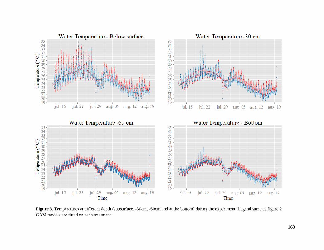
163

Figure 3. Temperatures at different depth (subsurface, -30cm, -60cm and at the bottom) during the experiment. Legend same as figure 2.

GAM models are fitted on each treatment.

164

165

Figure 5. Depth profiles of water temperatures in all mesocosms at two distinct dates at noon. The top

panel corresponds to temperatures taken on the 15th of July (without polyethylene films) and the bottom

panel corresponds to temperatures taken on august 15 (with polyethylene films). Mesocosms of the same

treatment group (3 mesocosms per treatment) share the same color.

166

Effect of warming on biotic and abiotic variables

Statistical analysis on the second period showed no significant effect of warming on any of

the 18 variables followed (See table 1 and figures 7, 8, 10). Considering the latter results, the

effect of mixing was tested on the whole data set and the warming effect was not taken into

account in the statistical models.

Effects of mixing on abiotic and biotic variables

Turbidity

Mixing increased the nephelometric turbidity

significantly (M, F1,10=10.30, p=0.0015, table

2). The highest turbidity values were found at

the bottom of mixed mesocosms and the lowest

values at the surface of calm mesocosms (Fig.

6). There was a clear difference between depths

with higher turbidity values at the bottom in

calm and mixed mesocosms (Depth,

F1,198=75.64, p<0.0001). The difference

between surface and bottom turbidity was more

important in mixed mesocosms compared to

calm ones (DxM, F1,198=9.176, p=0.0028).

Chemistry

No effect of mixing was detected on any of the chemical variables except for TOC (Fig.

7f). Nitrate-nitrogen concentration decreased rapidly from 2.13±0.25 mg L-1

to 0.67±0.15 mg L-1

during the first half (week 1- week 5, all mesocosms pooled) of the experiment and stabilized

Figure 6. Temporal dynamic of the

nephelometric turbidity (FNU). Black symbols :

mixed mesocoms, white symbols : calm

mesocoms. Round dots : surface measurements,

diamond shapes : bottom measurements. Error

bars are standard deviation. The decrease of

turbidity seen on the 4th week was due to an power

outage on the site that stopped the wave machines

for one or two days.

167

around 0.65 mg L-1

in the second half of the experiment (Fig. 7b). Nitrite-nitrogen followed the

same pattern with a rapid decrease from 0.029±0.006 mg L-1

to 0.009±0.007 mg L-1

in 5 weeks

and then stabilized (Fig. 7c). Ammonium remained at very low concentrations during the

experiment suggesting that the nitrogen cycle was functioning well (Fig. 7e). Total nitrogen

displayed an interesting temporal dynamic (Fig. 7a) with a decrease from 3.88±1.42 mg L-1

to

1.56±0.33 mg L-1

in the first half of the experiment in accordance with the decrease of nitrate-

nitrogen but then we observed a net increase from date 6 to 8 reaching concentrations of

3.79±0.79 mg L-1

while nitrate-nitrogen were still low suggesting a strong increase in

organically-bounded nitrogen. Total phosphorus showed a complex dynamic that we could not

successfully analyze with usual statistical method. Very high values were found in some

mesocosms, high above the original enrichment level of 0.1 mg L-1

suggesting that the sediment

and the water from Champ-Sur-Marne Lake were highly enriched in phosphorus. Total Organic

Carbon concentration almost doubled (from 14.42±1.43 mg L-1

to 26.42=0±1.94 mg L-1

, all

mesocosm pooled) in the first week of the experiment (Fig. 7f). Then, we observed a separation

between mixed and calm mescosoms with higher TOC concentrations in mixed mesocosms

compared to calm ones (MxT, F1,93=13.11, p=0.0005, table 2).

168

Table 1.Results of the warming experiment carried out in summer 2013.

P-values

Data set : 29/07-26/08

Response variable Mixing (M) Warming (W) Time (T) M x T WxT MxWxT

Turbidity

Nephelometric turbidity (FNU) 0.0476 n.s n.s. n.s n.s n.s.

Chemistry

Oxygen (mg L

-1) n.s n.s n.s. n.s. n.s. n.s.

pH n.s n.s n.s. n.s. n.s. n.s.

Ntot (mg L-1) n.s n.s <0.0001 n.s n.s n.s.

NO3-N (mg L-1

) n.s n.s n.s. n.s. n.s. n.s.

NO2-N (mg L-1

) n.s n.s <0.0001 n.s n.s n.s.

NH3-N (mg L-1

) n.s n.s n.s. n.s. n.s. n.s.

COT (mg L-1) 0.0592* n.s <0.0001 0.0565* n.s. n.s.

PO43-

(mg L-1

) not applicable

Phytoplankton

Chlorophyll YSI (µg Chl a L

-1) 0.0512* n.s 0.0035 n.s. n.s. n.s.

Green algae (µg Chl a L-1

) 0.0449 n.s 0.0053 n.s. n.s. n.s.

Blue green algae (µg Chl a L-1

) 0.0804 n.s. 0.0053 n.s. n.s. n.s.

Zooplankton

Zooplankton (ind. L

-1) n.s. n.s. n.s. n.s. n.s. n.s.

Rotifer (ind. L-1

) n.s. n.s. 0.0067 n.s. n.s. n.s.

Bosmina (ind. L-1

) n.s. n.s. <0.0001 n.s. n.s. n.s.

Nauplii (ind. L-1

) n.s. n.s. 0.0065 n.s. n.s. n.s.

Diaphanosoma Brachyurum n.s n.s 0.0217 n.s n.s n.s.

Copepode (ind. L-1

) n.s. n.s.

<0.0001 <0.0001 n.s. n.s.

n.s = not significant, * marginally significant.

169

Table 2.Results of mixing experiment carried out in summer 2013.

P-values

Data set : 01/07 - 26/08

Response variable Mixing (M) Time (T) Depth (D) M x T M x D D x T M x D x T

Turbidity

Nephelometric turbidity (FNU) 0.0079 0.0015 <0.0001 0.0004 0.0028 0.0001 n.s

Chemistry

Oxygen (mg L

-1) n.s. <0.0001 n.s. 0.0665* n.s. n.s. n.s.

pH 0.0477 <0.0001 n.s. 0.0204 n.s. n.s. n.s.

Ntot n.s <0.0001 n.s. 0.0621 n.s. n.s. n.s.

NO3-N (mg L-1

) n.s <0.0001 n.s. n.s. n.s. n.s. n.s.

NO2-N (mg L-1

) n.s <0.0001 n.s. n.s n.s. n.s. n.s.

NH3-N (mg L-1

) n.s n.s. n.s. n.s. n.s. n.s. n.s.

COT (mg L-1) 0.0336 <0.0001 n.s. 0.0005 n.s. n.s. n.s.

PO43-

(mg L-1

) not applicable

Phytoplankton

Chlorophyll a in situ (µg L

-1) 0.0648 <0.0001 <0.0001 0.0051 0.0101 0.0017 0.0562*

Green algae (µg Chl a L-1

) 0.0449 0.0001 n.s. 0.0083 n.s. n.s. n.s.

Blue-green in situ (µg Chl a L-1

) 0.0556* 0.0001 0.0001 0.0021 0.0259 0.0160 n.s.

Zooplankton

Zooplankton (ind. L

-1) n.s. <0.0001 n.s. n.s. n.s. n.s. n.s.

Rotifer (ind. L-1

) n.s. <0.0001 n.s. n.s. n.s. n.s. n.s.

Bosmina (ind. L-1

) 0.0188 <0.0001 0.0002 0.086 n.s 0.0329 n.s.

Diaphanosoma brachyurum n.s <0.0001 0.0099 0.053* n.s. n.s. n.s.

Nauplii (ind. L-1

) 0.0624* <0.0001 n.s. 0.0120 n.s. n.s. n.s.

Copepode (ind. L-1

) n.s <0.0001 n.s.

0.0001 n.s. n.s. n.s.

n.s = not significant, * marginally significant.

170

171

Effects of mixing on chlorophyll a, pH of dissolved oxygen

According to the BBE data, green algae chlorophyll a content accounted for more than 98%

of total chlorophyll a during the experiment. Diatoms and cyanobacteria signals were very low,

most of the time below detection limit. In contrast, the ISY probe gave a clear, positive dynamics

for blue-green algae, even though they still represented less than 6% of the total chlorophyll a

measured.

Green algae density increased rapidly during the first 5 weeks followed by a decline until

the end of the experiment (Fig. 8). Green algae reached higher density and decreased less rapidly

in mixed mesocosms compared to calm ones (MxT, F1,93=7.28, p=0.0083, table 2).

BBE and YSI measurements yielded comparable results in terms of global dynamic and

range of chlorophyll a concentration (linear regression : R²=0.62, p<0.0001) (Fig. 8a, b).

However, in situ data from the YSI probe showed a difference of chlorophyll a between the

surface and the bottom measurements (D: F1,197=36.67, p<0.0001). Detailed observations of the

dynamics of chlorophyll a in each mesocosms show that concentrations are homogeneous in calm

mesocosms while chlorophyll a concentrations were always higher at the bottom than at the

surface in mixed mesocosms (data not shown, MxD: F1,197=6.75, p=0.0151 and MxDxT:

F1,197=3.68, p=0.0562, table 2).

Blue-green algae measured with the YSI probe were positively affected by mixing and

grew better in mixed enclosures (Fig. 8c; MxT, F1,197=9.72, p=0.0021). They were more abundant

at the bottom of the enclosures (D: F1,197=36.67, p<0.0001), especially in mixed mesocosms

while they remained homogeneously distributed in calm enclosures.

172

The pH reached very high values during this experiment with an increase from 9.13±0.13 to

10.28±0.33 (all mesocosms pooled) in the first 4 weeks (Fig. 8d). Then, pH decreased in calm

mesocosm while it remained elevated in mixed mesocosms (MxT: F1, 93=5.56, p=0.0204, table 2).

Day-concentrations of dissolved oxygen were relatively high throughout the experiment.

Oxygen concentration in the water decreased steadily from the third to the sixth week and then

plateaued in both mixed and calm mesocosms (Fig. 8e). Dissolved oxygen (DO) concentrations

seemed to decrease to a lesser extent in mixed mesocosms but this effect was only marginally

significant (M x T: F1,92=3.44, p=0.0665, table 2). Night measurements (between 4 and 5 am)

were also done in August the night after day-measurements (6/08, 13/08 and 20/08) to evaluate

the effect of respiration on dissolved oxygen content at night (Fig. 9). The differential of

concentration between day and night measurements was significantly higher in mixed mesocosms

(Wilcox-test were performed on each date separately and yielded the following results date 6:

n=12 p=0.0076; date 7: n=12 p=0.0193; date 8: n= 12 p=0.0166, see figure 8).

Figure 9. Difference between day and night

concentration of dissolved oxygen (DO) in the

water. Measurements were done on three dates in

August. The night-measurements were done the

night after the day-measurements between 4 and 5

am. Round dots in boxplots represents the mean.

173

174

Effects of mixing on zooplankton

The zooplankton community was composed of 3 major groups : rotifers with large

dominance of the polyarthra, lecanidae and trichocera families, cladocerans with two prevalent

species Bosmina longirostris and Diaphanosoma brachyurum, and last, copepodes (large

dominance of cyclopides) and their nauplii larvae.

Rotifers were the only abundant zooplankton group for the first 4 weeks of experiment

(Fig. 10a). Their population dropped in mixed and calm mesocosms from 642±236 to 114±58

ind. L-1

in the first 3 weeks. Rotifers reached a peak of abundance on the fifth week (867±498

and 419±262 ind. L-1

in calm and mixed mesocosms, respectively) and then declined and

stabilized. Mixing had no noticeable effects on rotifer dynamics or abundance except that the

peak of abundance was slightly more important in calm mesocosms (wilcox-test on week 5, n=6

p=0.0465).

Cladocerans (B. longirostris and D. brachyurum) became relatively abundant in the second

part of the experiment (Fig. 10b, e). B. longirostris abundance was always higher at the bottom of

the water column than at the surface (D: F1, 102=14.55 p=0.0002, table 2). No significant effect of

mixing was found for either species dynamics.

Nauplii and cyclopide copepods also became noticeable in the second part of the

experiment (Fig. 10c, d). Mixing had a significant negative effect on both age classes (Nauplii: M

x T: F1, 70=6.65, p=0.0120; Copepodes: M x T: F1, 70=18.29 p=0.0001, table 2).

175

176

Discussion

Use of polyethylene films as a warming tool

To our knowledge, only two other warming experiments used a similar heating system

based on local green-house effect in aquatic mesocosm experiments (Strecker et al., 2004, Netten

et al., 2010). This system presents multiple advantages: 1/ this is a simple and cheap method, 2/

polyethylen films do not modify the sun spectrum, 3/ the warming of the water column comes

from the top as in natural systems 4/ the plastic films do not interfere with the structure of the

water column as immersed resistances or hot water injection would. This last point deserves some

emphasis as spatial heterogeneity is often overlooked in shallow ecosystems. In warmer climate,

the heat will come from the top of the water column and diffuse. Even if shallow lakes do not

experience strong and long-term stratifications, it is virtually certain that temperatures at the

surface will be higher than the temperatures at the bottom of the lakes. This difference of a few

degrees might be absolutely crucial to the species survival. Migration and patchiness are common

in freshwater and marine ecosystems. In this experiment, we noticed a clear pattern in the spatial

distribution of B. longirostris and D. brachyurum which were always more abundant at the

bottom than at the surface of our enclosures. Whatever the reason for this behavior, it indicates

that vertical distributions are not homogenous even in shallow environments. Homogeneously

warming mesocosms from the bottom might impair migration mechanisms to take place. It might

also unrealistically disturb the benthic fauna and chemical reactions at the water-sediment

interface like the release of phosphorus or deoxygenation.

177

On the (non)-effects of experimental warming

No significant effect of warming was found on any of the 18 variables followed during this

experiment. The statistical power of our analysis was greatly reduced by the fact that we had to

split the data set in half. Four weeks of warming did not seem enough to observe any sensible

effect of 1°C warming, especially on species such as copepodes which take a rather long time to

develop. Other warming experiment usually last for months or even years. Another important

point is that the month of July was especially hot this year for this region, with maximum water

temperatures around 35°C. Five fish died in calm enclosures during this period (1 on July 8th

, 3

on July 16 and 17th

, 1 on July 23rd

which was the hottest day); with no indication of disease

which suggests that they died from the heat or severe deoxygenation during the night. These

extreme temperatures in July might have selected very rapidly well-adapted species to warm

waters. Thus, the following 1°C warming might not have had any impact on neither selection nor

physiology of the species already in place. Very high temperatures might also have put pressure

on cladocerans and copepods which started to develop only after the atmospheric temperature

dropped at the end of July. Rotifers abundance also decreased rapidly during the first 3 weeks

while their food source (i.e phytoplankton) was increasing and their natural predators (mainly

copepodes here) were still absent which might indicate a negative effect of the July heatwave.

One degree Celsius warming is far below the usual temperature targets of warming

experiment in freshwater studies. However, before reaching 3 to 5°C warming, ecosystems will

go through a more or less continuous warming that should be addressed. 1°C warming

corresponds to predictions of the IPCC experts for the mid-century (3 out 4 climatic scenarios for

2046-2065). Will the response of freshwater ecosystems be gradual or will it be sudden? Is there

a temperature threshold that will trigger the changes observed today in warming experiments?

178

Will communities be able to evolve or at least adapt? New approaches with gradual temperature

increase seem necessary in order to understand how present-day communities will respond to

gradual warming. Implementing a sudden 3°C to 5°C temperature increase on present-day

community assemblages might relate more to heatwaves than long-term changes in average

temperatures.

Effects of mixing – comparison with 2012 experiment

Mixing had a noticeable impact on our mesocosms by increasing global turbidity and

mixing the whole water column. Higher concentrations of chlorophyll a, TOC, pH values and

oxygen concentrations suggests that the standing crop of autotrophic organisms was greater in

mixed enclosures. The difference between day and night oxygen concentrations was significantly

greater in mixed enclosures supporting the idea that mixing allows the system to have higher

global biomass.

Higher concentrations of chlorophyll a can be due to 1/ increased abundance of

phytoplankton 2/ at similar abundance: bigger cells with higher chlorophyll a content or 3/ for the

same size and abundance: higher concentration of chlorophyll per cells. Our data set does not yet

allow us to differentiate between those 3 possibilities. However, in a previous mixing experiment

(Blottière et al. submitted), we showed that higher chlorophyll a concentrations were not

attributable to increased abundance of phytoplankton. It seems rather that cells had higher content

of chlorophyll a suggesting physiological adaptation to mixing. As in 2012, we also observe

increased pH values in our mixed enclosure, again suggesting increased withdrawal of CO2 due

to higher photosynthetic activity. The hypothesis developed in the previous experiment was that

by circulating regularly in the whole water column, phytoplankton had regular access to high

light intensity but was less likely to suffer from photoinhibition due to surface high irradiance.

179

Nutrient availability was not affected by mixing. We did not observe higher release of

phosphorus in mixed mesocosms despite the addition of enriched sediments. It is possible that

with the important temperature experienced in July, most of the phosphorus held in the sediment

was rapidly released in the water in all mesocosms, and the effect of mixing was therefore

negligible compared to diffusion from the sediments (Jensen and Andersen 1992; Søndergaard et

al. 2003; Jensen et al. 2006).

Copepodes and nauplii were the only zooplankton group to significantly respond to mixing.

Adult and nauplii grew better in calm enclosures. Whether the mixing negatively impacted

nauplii, adults or both remains uncertain. Many nonexclusive hypotheses may be proposed to

explain this result: 1/ a negative effect of turbidity on nauplii and copepodes hunting skills, 2/

physical interference of mixing which could increase energy expenditures, 3/ higher turbidity

could impair copepodes detection of their predators.

Altogether, the results of this experiment are remarkably similar to results obtained with the

mixing experiment carried out in 2012 (Blottière et al. in prep.). The only major difference with

2012 is the effect of mixing on nitrites. In 2012, nitrites accumulated in calm and mixed

mesocosms, but significantly less in mixed mesocosms. In 2013, nitrites were at very low

concentration throughout the experiment. This comparison suggests that in 2012, there was a

general dysfunction of the nitrogen cycle which led to nitrite accumulation, and in that case,

mixing tended to reduce this accumulation. This dysfunction was likely due to the fact that tanks

were filled with tap water, which lacked nitrogen cycling bacterial communities. This was not the

case in 2013 as the water came at 50% from a local reservoir with a well-established nitrogen

cycle.

180

Despite differences in enrichment (being more important in 2013 than in 2012), timing

(2012: August-September 2013: July-August) and overall biomass (higher in 2013 than in 2012)

the effect of mixing seems robust and repeatable.

Conclusion

Our experiment was not long enough to observe any subtle change in communities

responses due to 1°C increase. More experiments with gradual increases of temperatures are

necessary to comprehend how freshwater communities will respond to the future changes in

average temperatures. On the other hand, this experiment strongly support the idea that mixing is

an important element in shallow lake functioning. Lake to lake variability or even intra-lake

variability might come in part from different wind-exposure and mixing intensity. Further studies

are needed to fully comprehend how different structural parameters will interact with an increase

in global temperatures.

Aknowledgments

We wish to thank François Rocher and Jean-Jacques Lamandé of the CEREEP Ecotron

station for their technical help regarding the repairs, maintenance and setting up of the ramps on

the enclosures. We also thank the CNRS station for their help and technical support. L.B. and this

work are financially supported by the ANR Pulse 2010 CEPL 01004 and the ANR Equipex

PLANAQUA (ANR-10-EQPX-13-01) coordinated by the CEREEP-Ecotron IleDeFrance (UMS

3194).

181

References

Blottière, L., M. Rossi, F. Madricardo, and F. D. Hulot. 2013. Modeling the role of wind and

warming on Microcystis aeruginosa blooms in shallow lakes with different trophic status.

Theor. Ecol. 7: 35–52.

Blottière, L., S. Jacquet, A. Millot, and F. D. Hulot. (submitted). How does mixing affect the

pelagic food-web in shallow lakes?

Carrick, H. J., F. J. Aldridge, and C. L. Schelske. 1993. Wind influences phytoplankton biomass

and composition in a shallow, productive lake. Limnol. Oceanogr. 38: 1179–1192.

Dodds, W. K., W. W. Bouska, J. L. Eitzmann, T. J. Pilger, K. L. Pitts, A. J. Riley, J. T.

Schloesser, and D. J. Thornbrugh. 2009. Eutrophication of U.S. freshwaters: analysis of

potential economic damages. Environ. Sci. Technol. 43: 12–19.

IPCC, 2014: Climate Change 2014: Synthesis Report. Contribution of Working Groups I, II and

III to the Fifth Assessment Report of the Intergovernmental Panel on Climate Change [Core

Writing Team, R.K. Pachauri and L.A. Meyer (eds.)]. IPCC, Geneva, Switzerland, 151 pp.

Feuchtmayr, H., R. Moran, K. Hatton, L. Connor, T. Heyes, B. Moss, I. Harvey, and D. Atkinson.

2009. Global warming and eutrophication: Effects on water chemistry and autotrophic

communities in experimental hypertrophic shallow lake mesocosms. J. Appl. Ecol. 46: 713–

723.

Gyllström, M., L. -a. Hansson, E. Jeppesen, F. García-Criado, E. Gross, K. Irvine, T. Kairesalo,

R. Kornijow, M. R. Miracle, M. Nykänen, and T. Nöges. 2005. The role of climate in

shaping zooplankton communities of shallow lakes. Limnol. Oceanogr. 50: 2008–2021.

Huisman, J., P. van Oostveen, and F. J. Weissing. 1999. Species Dynamics in Phytoplankton

Blooms: Incomplete Mixing and Competition for Light. Am. Nat. 154: 46–68.

Huisman, J., J. Sharples, J. M. Stroom, P. M. Visser, W. E. a. Kardinaal, J. M. H. Verspagen, and

B. Sommeijer. 2004. Changes in Turbulent Mixing Shift Competition for Light Between

Phytoplankton Species. Ecology 85: 2960–2970.

Hulot, F. D., G. Lacroix, and M. Loreau. 2014. Differential responses of size-based functional

groups to bottom-up and top-down perturbations in pelagic food webs: a meta-analysis.

Oikos 001–010.

Jensen, H. S., and F. O. Andersen. 1992. Importance of temperature, nitrate, and pH for

phosphate release from aerobic sediments of four shallow, eutrophic lakes. Limnol.

Oceanogr.

Jensen, J. P., A. R. Pedersen, E. Jeppesen, and M. Søndergaard. 2006. An empirical model

describing the seasonal dynamics of phosphorus in 16 shallow eutrophic lakes after external

loading reduction. Limnol. Oceanogr. 51: 791–800.

182

Jeppesen, E., M. Søndergaard, J. P. Jensen, K. E. Havens, O. Anneville, L. Carvalho, M. F.

Coveney, R. Deneke, M. T. Dokulil, B. Foy, D. Gerdeaux, S. E. Hampton, S. Hilt, K.

Kangur, J. Köhler, E. H. H. R. Lammens, T. L. Lauridsen, M. Manca, M. R. Miracle, B.

Moss, P. Nõges, G. Persson, G. Phillips, R. Portielje, S. Romo, C. L. Schelske, D. Straile, I.

Tatrai, E. Willén, and M. Winder. 2005. Lake responses to reduced nutrient loading - An

analysis of contemporary long-term data from 35 case studies. Freshw. Biol. 50: 1747–

1771.

Kratina, P., H. S. Greig, P. L. Thompson, T. S. a Carvalho-Pereira, and J. B. Shurin. 2012.

Warming modifies trophic cascades and eutrophication in experimental freshwater

communities. Ecology 93: 1421–1430.

Liboriussen, L., F. Landkildehus, M. Meerhoff, M. E. Bramm, M. Søndergaard, K.

Christoffersen, K. Richardson, M. Søndergaard, T. L. Lauridsen, and E. Jeppesen. 2005.

Global warming: Design of a flow-through shallow lake mesocosm climate experiment.

Limnol. Oceanogr. Methods 3: 1–9.

Lürling, M., F. Eshetu, E. J. Faassen, S. Kosten, and V. L. M. Huszar. 2013. Comparison of

cyanobacterial and green algal growth rates at different temperatures. Freshw. Biol. 58:

552–559.

Mckee, D., D. Atkinson, S. Collings, J. Eaton, I. A. N. Harvey, K. Hatton, T. O. M. Heyes, D.

Wilson, L. Wolstenholme, and B. Moss. 2000. Heated aquatic microcosms for climate

change experiments. 51–58.

McKee, D., D. Atkinson, S. E. Collings, J. W. Eaton, a. B. Gill, I. Harvey, K. Hatton, T. Heyes,

D. Wilson, and B. Moss. 2003. Response of freshwater microcosm communities to

nutrients, fish, and elevated temperature during winter and summer. Limnol. Oceanogr. 48:

707–722.

Meerhoff, M., J. M. Clemente, F. T. de Mello, C. Iglesias, A. R. Pedersen, and E. Jeppesen. 2007.

Can warm climate-related structure of littoral predator assemblies weaken the clear water

state in shallow lakes? Glob. Chang. Biol. 13: 1888–1897.

Mette, E. M., M. J. Vanni, J. M. Newell, and M. J. González. 2011. Phytoplankton communities

and stoichiometry are interactively affected by light, nutrients, and fish. Limnol. Oceanogr.

56: 1959–1975.

Mooij, W. M., S. Hülsmann, L. N. De Senerpont Domis, B. a. Nolet, P. L. E. Bodelier, P. C. M.

Boers, L. M. D. Pires, H. J. Gons, B. W. Ibelings, R. Noordhuis, R. Portielje, K. Wolfstein,

and E. H. R. R. Lammens. 2005. The impact of climate change on lakes in the Netherlands:

a review. Aquat. Ecol. 39: 381–400.

Moss, B., D. Stephen, D. M. Balayla, E. Becares, S. E. Collings, C. Fernandez-Alaez, M.

Fernandez-Alaez, C. Ferriol, P. Garcia, J. Goma, M. Gyllstrom, L. -a. Hansson, J. Hietala,

T. Kairesalo, M. R. Miracle, S. Romo, J. Rueda, V. Russell, a. Stahl-Delbanco, M.

183

Svensson, K. Vakkilainen, M. Valentin, W. J. Van de Bund, E. Van Donk, E. Vicente, and

M. J. Villena. 2004. Continental-scale patterns of nutrient and fish effects on shallow lakes:

synthesis of a pan-European mesocosm experiment. Freshw. Biol. 49: 1633–1649.

Netten, J. J. C., G. H. P. Arts, R. Gylstra, E. H. van Nes, M. Scheffer, and R. M. M. Roijackers.

2010. Effect of temperature and nutrients on the competition between free-floating Salvinia

natans and submerged Elodea nuttallii in mesocosms. Fundam. Appl. Limnol. / Arch. für

Hydrobiol. 177: 125–132.

Reynolds, C. S. 2006. The Ecology of Phytoplankton, Press, Cambridge University.

Reynolds, C. S., S. W. Wiseman, and M. J. O. Clarke. 1984. Growth- and loss-rate responses of

phytoplankton to intermittent artificial mixing and their potential application to the control

of planktonic algal biomass. J. Appl. Ecol. 21: 11–39.

Reynolds, C. S., S. W. Wiseman, B. M. Godfrey, and C. Butterwick. 1983. Some effects of

artificial mixing on the dynamics of phytoplankton populations in large limnetic enclosures.

J. Plankton Res. 5: 203–234.

Schelske, C. L., H. J. Carrick, and F. J. Aldridge. 1995. Can wind-induced resuspension of

meroplankton affect phytoplankton dynamics? J. N. Am. Benthol. Soc. 14: 616–630.

Sommer, U., R. Adrian, L. De Senerpont Domis, J. J. Elser, U. Gaedke, B. Ibelings, E. Jeppesen,

M. Lürling, J. C. Molinero, W. M. Mooij, E. van Donk, and M. Winder. 2012. Beyond the

Plankton Ecology Group (PEG) Model: Mechanisms Driving Plankton Succession. Annu.

Rev. Ecol. Evol. Syst. 43: 429–448.

Søndergaard, M., J. P. Jensen, and E. Jeppesen. 2003. Role of sediment and internal loading of

phosphorus in shallow lakes. Hydrobiologia 506-509: 135–145.

Stewart, R. I. a, M. Dossena, D. a. Bohan, E. Jeppesen, R. L. Kordas, M. E. Ledger, M. Meerhoff,

B. Moss, C. Mulder, J. B. Shurin, B. Suttle, R. Thompson, M. Trimmer, and G. Woodward.

2013. Mesocosm Experiments as a Tool for Ecological Climate-Change Research, 1st ed.

Elsevier Ltd.

Strecker, A. L., T. P. Cobb, and R. D. Vinebrooke. 2004. Effects of experimental greenhouse

warming on phytoplankton and zooplankton communities in fishless alpine ponds. Limnol.

Oceanogr. 49: 1182–1190.

Yvon-Durocher, G., J. I. Jones, M. Trimmer, G. Woodward, and J. M. Montoya. 2010. Warming

alters the metabolic balance of ecosystems. Philos. Trans. R. Soc. Lond. B. Biol. Sci. 365:

2117–2126.

Yvon-Durocher, G., J. M. Montoya, M. Trimmer, and G.Woodward. 2010. Warming Alters the

Size Spectrum and Shifts the Distribution of Biomass in Aquatic Ecosystems. Glob. Chang.

Biol. 17 pp.1681.

184

Annexe 1

Natural light spectra. Blue : direct sunlight. Green : 100µm polyethylen film. Pink : 200µm

polyethylen film.

185

Conclusion and perspectives

186

187

During the last four years, we have documented the effects of wind-induced mixing on

pelagic communities in shallow lakes with modeling and experimental approaches. Throughout

this work, we included two anthropogenic stressors: nutrient enrichment and increased

temperatures in order to integrate ongoing changes in freshwater ecosystems.

One of the challenges of ecological studies is to understand the intricate relationships

between abiotic and biotic drivers in the organization of communities, foodwebs and on a larger

scale, the functioning of ecosystems. In this regard, freshwater lakes are particularly interesting

models since a great deal of knowledge has been accumulated on their physical structure as well

as on the composition and organization of their foodwebs (Strong 1992, Chase 2000, Hulot et al.

2000, Shurin et al. 2006). In freshwater environments, foodwebs and communities are shaped by

biotic interactions such as predator-prey or allelopathic interactions but also by abiotic variables

such as light, temperature and of course mixing. However, for a long time, the representation of

these different drivers and interactions lacked a general framework.

Recently, Olff and his colleagues (2009) proposed new frameworks in which multiple kinds

of interactions could be represented in addition to predator-prey interactions. Typically, the first

framework they proposed (Figure 12), allows for the inclusion of an abiotic factor and its effects

on the rest of the foodweb. This kind of representation could prove to be particularly useful when

an abiotic factor is a strong driver of population dynamics with different responses for each

trophic level. In the light of previous studies and the results of this thesis, it seems clear that

wind-induced mixing is a key abiotic process driving shallow freshwater ecosystems through

direct and indirect pathways (Figure 7 in chapter III). In the following section, I will discuss the

results obtained during the last four years and the perspectives they offer for further studies. To

do so, I will first comment on my major experimental results and how they add to current

188

knowledge, then I will address the concept of temporality of wind-induced events, and finally, I

will discuss some questions raised by our warming experiment.

Figure 12. Framework proposed by Olff et al. 2009 allowing the inclusion of abiotic factors and various

types of interactions in foodweb representation.

189

Reproducibility and major experimental results

A key aspect of science is the reproducibility of experimental results. Often confused with

the notion of replicates, which is performed within an experiment, reproducibility is an

independent repetition of an experiment which gives similar results every time. The latter is a

necessary condition for establishing facts in any field of science. In 2012 and 2013 we carried out

two experiments with similar treatments regarding the mixing intensity. Both gave the same

results, and when divergence occurred, it was explained by the specificity of each year initial

conditions. For instance, in 2012 and 2013, mixing increased the chlorophyll a content in mixed

enclosures and had a negative impact on copepodes but we did not observe the same effect in the

consecutive years on nitrite-nitrogen. However, in 2012, there was a general dysfunction of the

nitrogen cycle leading to nitrite-nitrogen accumulation in calm and mixed enclosures. This

accumulation was alleviated by mixing, probably through a better oxygenation of the sediments

where most of the nitrification activity takes place. In 2013, there was no accumulation of nitrite-

nitrogen, therefore in this particular case, no effect of mixing was observed.

Effects of mixing on chlorophyll a content

Although two independent experiments are not enough, and this experiment should be

reproduced by other scientists, the fact that we observed similar patterns gives us confidence in

the experimental results. In 2012 and 2013, mixing had a positive effect on chlorophyll a

concentration in the water column. According to the literature on the subject, two mechanisms

could be behind this effect: (i) increased availability of nutrients in the water column, (ii)

phytoplankton cells are more abundant in the water column of mixed enclosures due to the

absence of loss rate via sedimentation. However, both hypotheses were rapidly ruled out as

nutrient content and phytoplankton cell counts were similar between treatments (phytoplankton

190

count-analyses for 2013 still underway). There was a clear discrepancy between cell counts and

chlorophyll a content suggesting a physiological adaptation of primary producers to either

turbidity or mixing or both. Changes in intracellular pigment content are characteristic of light-

shade adaptation in plants and phytoplankton (Beale & Appleman 1971, Falkowski & Owens

1980, Reynolds 2006 p. 113-114). Typically, phytoplankton cells respond to decreased light by

increasing their photosynthetic pigment content. Variations of cell pigment content between

individuals grown under different light intensity may vary from two up to -nine folds (Falkowski

1980, Reynolds 1997). Reynolds (2006 p. 113) states that most phytoplankton are able to adjust

their chlorophyll a content within a range of ±50% of average and so within one or two cell

generations. This capacity allows for the cell to adapt its harvesting capacity to light availability.

In turbid environment such as well-mixed shallow lakes, it is thus very likely to find higher

chlorophyll a content per cell compared to phytoplankton in wind-protected area.

The chlorophyll a content can also vary gapingly between different species. Using a large

data set of unpublished field measurements, Reynolds found in 1984 that biomass-specific

estimates of chlorophyll a content ranged from 0.0015 to 0.0197 pg µm-3

of live cell volume.

Felip & Catalan (2000) reported in a field study that differences in the taxonomic composition of

phytoplankton accounted for most of the variability in the chlorophyll-biovolume relationship. In

conclusion, in our experiment, the increase in chlorophyll a observed in mixed enclosures could

be due to (i) increased pigment synthesis as a mean of photoadaptation to higher turbidity caused

by resuspended materials, (ii) change in species composition toward species with higher

chlorophyll content. Further analysis of DNA sampled during our experiment might help

determine if one of these hypothesis or both is responsible for the discrepancy between algae

count and chlorophyll a concentration. In all, our results add to the debate on the utilization of

191

chlorophyll concentration as a proxy of phytoplankton biomass and productivity (Felip & Catalan

2000, Kruskopf & Flynn 2006).

Effect of fluctuating light on phytoplankton productivity

In our mesocosm experiments, pH was higher in mixed enclosures compared to calm ones.

In natural system, high pH is indicative of high photosynthesis activity depleting the water of its

dissolved inorganic carbon (Schelske & Callender 1970, Schelske et al. 1974, Heaney et al. 1986,

observed in Litchman 1998 and Feuchtmayr et al. 2009). Therefore we concluded that mixing

enhances photosynthetic activity. First, we thought that it was a direct consequence of higher

chlorophyll a content in phytoplankton cells; however, this is not likely the case as cells with

higher chlorophyll content only compensate for the reduced light availability caused by turbidity.

In theory, these cells are capable of fixing the same amount of carbon as cells growing at higher

irradiance (Reynolds 2006 p. 144). The observed increase in photosynthetic activity is rather

linked to the regime of fluctuating light experience in mixed mesocosms.

An abundant literature exists on the physiology of phytoplankton in response to fluctuating

light experienced by cells in the mixing layer (Marra, 1978, Walsh & Legendre 1983, Falkowski

1984, Cullen & Lewis 1988, Kroon et al. 1992, Mallin & Paerl 1992, MacIntyre 1993, Litchman

1998, 2000). This was studied first on marine phytoplankton. In 1978, John Marra made an

experiment measuring the production of phytoplankton (via carbon-14 uptake rates) suspended in

bottles that were either fixed at a certain depth or moved through the water column. He found that

estimates of integral photosynthesis were 19 to 87% higher under variable light condition that

was probably explained by higher light-saturated photosynthetic rates. Traveling through the

water column may be an advantage as cells are regularly brought up to surface-light intensities

which allow phytoplankton to photosynthesize at light-saturated rates. In turn, they are unlikely

192

to suffer from photoinhibition as they are moved downward to lower irradiance layers (Ibelings et

al. 1994). Similarly, algae are very unlikely to be light-limited as might be the case for

sedimented algae in calm waters (Mallin & Paerl 1992). In all, rapid light fluctuations due to

continuous mixing might generate optimal conditions for photosynthetic activity. Nevertheless,

precise monitoring and physiological measurements would be necessary in further studies to

validate these hypotheses.

Interestingly, some studies suggest that phytoplankton species are unequally adapted to

fluctuating light. In an impressive study, Ibelings et al. (1994) compared the responses of

cyanobacterium M. aeruginosa and the green algae Scenedesmus protuberans to simulated

fluctuating light corresponding to wind-induced mixing. They concluded that S. protuberans was

more flexible in its acclimation to fluctuating lights compared to the cyanobacterium which

relates well to their specific strategies regarding buoyancy and vertical placement. In 1998, Elena

Litchman studied the impact of fluctuating light on the diversity, composition and structure of 2

and 18-species communities of freshwater phytoplankton. She showed that diatoms were favored

under fluctuating light where they became the dominant group. This positive effect of fluctuating

light on growth of diatoms add to the already known positive effect of mixing which keeps these

heavy cells suspended in the water column. This was not observed in our mixed enclosures where

densities of diatoms remained very low throughout the experiment. However, other elements

such as initial input and climatic conditions were probably unfavorable to diatoms. Litchman

(1998, 2000) also added that the very species-specific growth rates responses to fluctuating light

could be of major importance for differences in community composition in natural systems. As

mentioned previously, analysis of DNA samples could give us further information on whether

mixing impacted species composition and diversity in our mesocosm experiments.

193

Effects of mixing on zooplankton communities

In our studies, we monitored not only the response of phytoplankton to mixing but also the

responses of other functional groups, especially zooplankton. In 2012 as well as in 2013,

copepodes were the only group affected (negatively) by mixing. With our data set, it was not

possible to give a specific mechanism behind this negative effect, however, we could speculate

direct physical disturbance on copepodes kinematics, which could be energy-consuming and lead

to lower growth rates (Yen et al. 2008). Indirect effect through turbidity and suspended material

could also be responsible for lower food quality, with a proportionally higher consumption of

resuspended materials with low nutritional value (Paffenhöfer 1972, Gasparini et al. 1999),

and/or lower feeding rates due to interference of resuspended material on copepods hunting

capacity (Levine et al. 2005).

In 2012, I suspected the difference in copepod density in the second half of the experiment

to be responsible for the shift in population maxima of rotifers. In calm enclosures where

copepods were more abundant, rotifer population decreased earlier than in mixed enclosures.

Copepods are known to exert a strong top-down control on rotifers as they are usually considered

as their favorite preys (Brandl 2005). This could be an interesting outcome of mixing on the

organization and force of feeding links in the foodweb. However, this result is uncertain as this

pattern was not clearly observed in 2013.

Effects of mixing on bacteria and viruses

Our analysis also showed a difference in the lysis activity of virus on prokaryotes

depending on the mixing regime. In contrast to calm enclosures where lysis activity remained low

and rather homogenous, we observed a high peak of lysis activity in the three mixed mesocosms.

This could be the result of a higher contact rate between the viruses and their hosts. In the last

194

decades, the impacts of viruses on foodwebs and community organization have sparked the

interests of the scientific community. For instance, viruses have been shown to be a major control

agent of phytoplankton blooms (Jacquet et al. 2002, Frada et al. 2008, review in Paerl & Otten,

2013). Hudnell et al. (2010) proposed that one of the mechanisms through which artificial mixing

controlled harmful algal blooms was the promotion of cyanophage distribution in the water

column. Our results support the idea that communities in well-mixed water bodies could be

subjected to stronger regulation by pathogens such as viruses.

In conclusion, our experiment brought additional informations on the impact of wind-

induced mixing on pelagic communities. Usual effects, such as benthic recruitment or important

releases of nutrients from the sediment bed were not observed due to the time-scale and set-up of

mesocosms. However, this allowed us to uncover important effects of mixing on phytoplankton

physiology and photosynthetic activity. Furthermore, we showed that other compartment of the

foodweb were also sensitive to mixing with differential responses among groups. Here only

copepods responded with a possible top-down consequence on rotifers while cladocerans

remained undisturbed. In addition, virus-prokaryote interaction seemed enhanced by mixing and

deserves more emphasis in further studies. Furthermore, there is still a huge gap of knowledge on

the microbial community and activity which needs further analysis.

Temporality of wind-induced mixing episodes

In our modeling and field studies, mixing was applied continuously on our systems, except

for simulations of storm events with net changes in wing regimes. In natural environments, the

frequency and length of wind-induced mixing episodes may be highly different depending on the

lakes morphometry, exposure and location. On coastal region and/or in very large lakes with

195

important fetch and low depth, mixing might be almost continuous whereas in less exposed

regions, wind-induced mixing may be less frequent with long pauses between windy episodes.

The frequency of resuspension events is of great importance to the sediment structure.

Long-lasting calm periods will allow sediment deposition and consolidation. The stability of the

sediment cohesion depends to a large extent on chemical factors such as electrostatic attraction

caused by ion pairing, which modulates sediment flocculation processes (Lundkvist et al. 2007).

In addition, given enough time between windy episodes, bacteria, microalgae and fungi may form

biofilms at the surface of the sediments that increase the erosion threshold, decrease erosion rates

and enhance deposition (Grant et al. 1986, Madsen et al. 1993, Lundkvist et al. 2007, Righetti &

Lucarelli 2010, Fang et al. 2014, Ubertini et al. 2015). Also, bacteria within the sediment matrix

can also promote the binding of the sediment via the excretion of extracellular polymers. For

instance, in an experiment analyzing the contribution of physical-chemical factors and

microbiobial factors on marine sediment cohesion, Lundkvist et al. 2007 found that the presence

of benthic diatoms increased the erosion threshold by 120% and bacteria by 20%. When both

were present, this threshold was increased by 150% suggesting synergistic effects. After a

mechanical disturbance of the sediment, 10 days were necessary to reach a plateau of sediment

stability. As we have seen previously, the sediment is also a reservoir of nutrients, especially

phosphorus in shallow ecosystems. In the case of intermittent resuspension, wind events will

have a stronger impact on phosphorus release as concentration gradients between the sediments

and the water column will have time to establish between resuspension events (Søndergaard et al.

1992).

In some cases, wind has a specific pattern. In a very well documented and interesting paper,

Arfi & Bouvy (1995) described the clear diel wind cycle experienced by the tropical shallow

196

Ebrié lagoon in Côte d‟Ivoire. From midnight to midday, the wind blows at low speed (~1.2 m s-

1), the water is flat and sedimentation occurs whereas from midday to midnight, the wind blows

at higher speeds (>3 m s-1

, range: 4-6 m s-1

), waves form and resuspension of sedimented

particles takes over. The authors showed that this pattern was the main physical factor controlling

the pelagic ecosystem. For instance, daily changes in nutrient content (specifically NH4-N and

PO4-P) were due to resuspension of algae cells, which led to increased uptake during windy

episodes. When the wind speed decreased, nutrient standing stock reconstituted rapidly. They

also demonstrated that the size distribution of bacterial cells changed with windy episodes as

large benthic bacteria were brought into the water column. Similarly, the composition of

phytoplankton communities temporarily changed with higher proportion of diatoms, chlorophytes

such as Chlorella sp. and some species of cyanobacteria. Particle size was greatly influenced by

the wind, and small particles stayed longer than heavy and large particles during the relaxation

period. The authors hypothesized that all these changes were likely to modify the food-web

organization on a short time-scale with regular formation or suppression of feeding links.

Micrograzers (like ciliates) seemed permanently favored as small size-particles (small bacteria

and picoalgae) were regularly resuspended and stayed longer in the water column, while the food

resource of predators feeding on larger particles were dependent on resuspension event and

length.

Rapid shifts in community structure have also been observed in Lake Balaton in Hungary

due to storm events. Padisák (1988, 1990) showed that storm events occurring after 5-15 days of

calm weather cause “jump-like” changes in phytoplankton community composition with a rapid

growth of small algae that last for a few days, which are then replaced by larger algae until the

next storm. Furthermore, the dominant filamentous cyanobacteria significantly decreased because

197

of the storm. The explanation given by the authors was physiological death of cells of unknown

cause. However, one may think of direct physical effect of strong small-scale turbulence on the

structure of filaments or mechanical damage due to collision with other particles (Moisander et

al. 2002). Resuspension events can also induce loss of pelagic phytoplankton biomass through

aggregation (also called flocculation) between cells and sediment particles such as clay

(Avnimelech et al. 1982). This process is driven in part by mass action, i. e. the flocculation rate

is proportional to concentration of suspended particles, in part by the type of clay (size and

surface charges), and also by the “stickiness” of the phytoplankton species. The latter is often

linked to the amount of extracellular polymers excreted by algae, such as mucilage (Walsby

1968, Kiørboe & Hansen 1993). This mechanism may even cause buoyant species to sediment.

For instance, Verspagen et al. (2004, 2006) showed that aggregation with clay particles was the

main mechanism behind Microcystis spp. sedimentation in Lake Volkerak (The Netherlands).

As knowledge of freshwater ecosystem accumulates, it becomes clear that physical factors

such as wind events are a key process driving those ecosystems. Continuous mixing in well-

exposed lakes generates specific conditions of turbidity and fluctuating light that will affect the

phytoplankton as well as zooplankton. Periodic wind events act as “pulses” that can change the

underwater light climate and nutrient availability as well as the organization and composition of

planktonic communities. With our mesocosm experiment, we studied only one kind of mixing

pattern, but storm events, intermittent wind episodes with varying time-lags and diel patterns are

also among the possible scenarios that could be explored. In addition, different kinds of

sediments could also be used to determine the importance of sediment composition in

resuspension events.

198

Warming – results and questions

In 2013, we crossed a mixing treatment with a warming treatment using polyethylen films

to produce local greenhouse effects. Originally, the warming was supposed to start at the

beginning of the mixing treatment; however, due to delays in the delivery of polyethylen sheets,

it only began halfway through the experiment. This led to a short-term warming effect of 4 weeks

which, compared to other warming experiments, is quite short. In addition, the polyethylen sheets

were specifically made to fit on our mesocosms and we had no previous knowledge on the

intensity of warming we would get. Post-experiment quantification of warming indicated that the

greenhouse effect led to a temperature rise of ~1°C throughout the water column. This increase

was surprisingly well-maintained until the end of the experiment, suggesting that equilibrium

between the greenhouse effect and temperature exchanges with the atmosphere was reached.

Does the fact that we did not observe any effect of 1°C warming mean that there is none?

This is quite unlikely. Most of freshwater species, from bacteria to phytoplankton, to zooplankton

and fish, have temperatures optimum for growth, reproduction and steps in life-cycles. These

optimums correspond to hardwired metabolic activities and rates. In nature, there are increasing

evidences that relatively small increases in temperature (0.6°C in the past 100 years) can affect

phenological events (Walther et al. 2002). For example, flowering and bud-breaking in plants

tend to happen earlier in spring (1.4-3.1 days earlier per decade in Europe), butterflies appear

earlier (2.8-3.2 days per decade) and amphibians and birds also breed earlier. In freshwater

ecosystems, the timing and magnitude of seasonal phytoplankton blooms are also shifting in

response to recent climate changes (Thackeray et al. 2010, Winder et al. 2012). In our modelling

work, we also found that blooms of M. aeruginosa happen sooner in summer with 2°C warming

due to a physiological advantage at higher temperatures. Herbivores, such as the key-stone

199

species of the genus Daphnia are also known to be strongly regulated by water temperatures and

respond to higher temperatures by reaching their maximum density sooner (Thackeray et al.

2012, Straile et al. 2012). In our experiment, time was a limiting factor and phenological changes

could not be observed due to the experimental time scale. However, changes in community

assemblages (for example an increase in abundance of cyanobacteria relative to green algae) and

changes in abundance of fast-growing organisms such as phytoplankton, rotifers and bosmines

were expected (Strecker et al. 2004, Walters et al. 2013). We did not observe any changes on

community assemblages with the present data set however, phytoplankton and bacteria counting

is still ongoing at the moment. Those groups with high turn-overs are the most likely to respond

to warming in short periods of time. Any effects on other groups with longer growth such as

copepods are unlikely to be detectable in short-term experiments.

In order to better anticipate the effects of global warming on shallow freshwater

ecosystems, many experiments have been carried out in mesocosms (McKee et al. 2003, Moss et

al. 2003, Strecker et al. 2004, Feuchtmayr et al. 2009, 2010, Kratina et al. 2012, Nicolle et al.

2012). Most of these experiments use complex heating systems, often fixed just above the

sediment, injecting hot (up to 60°C) water into the enclosures. The water temperature increase

targeted is often between 3 and 5°C above non-heated adjacent mesocosms, which is

considerable. These set-ups raise some questions on the effects produced. First, as we have seen,

the physical structure of shallow lake is key to many processes, and especially the interface

between the water column and the sediments. Injecting hot water or heating the systems from the

bottom just above the sediments is likely to disrupt important processes such as nutrient cycles,

phosphorus release, nitrification etc. Moreover, in nature, the warming comes from a greenhouse

effect from the atmosphere. The temperature dissipates throughout the water column and

200

gradients of temperature, even small, appear. For example, with our heating systems, we

observed a structure in temperatures in the water column even though the enclosures are only 1m

deep. This heterogeneity seems crucial, as it gives the possibility of vertical migration for some

species where they can find a relief from hot temperatures or, on the contrary, migrate to hotter

waters. In our experiment, we found that some species, especially cladocerans were not

distributed homogeneously with depth and were more abundant at the bottom of enclosures.

However, many hypotheses could explain this phenomenon: predation avoidance, hot

temperature avoidance, better access to food resources at the bottom etc.

Another question that should be raised concerning experimental warming in mesocosm is

what are we testing when we apply 3 to 5°C of warming to present-day communities? According

to the 2014 IPCC reports, these temperature increases will be reached at the end of the 21st

century. Before then, global average temperatures will increase in an almost linear fashion as in

figure 13.

201

Many changes in processes, communities‟ organization and phenology will probably occur

during the next 85 years in response to small, gradual increases in temperatures. Acclimation,

adaptation and evolution will also take place (Parmesan 2006). It would be interesting to make

controlled experiments with smaller increases in temperature and also investigate what are the

responses of communities to slow, gradual increases rather than abrupt and considerable

temperatures increases.

General conclusion

Wind-induced mixing plays a major role on freshwater ecosystems. From physiological

adaptations of phytoplankton cells to fluctuating light to changes in diversity, community

successions and foodweb organization, water column mixing affects water bodies through

multiple pathways. Intra-lake variability of wind-exposure could generate patchiness in the

community composition and foodweb organization. For instance, we could speculate that

biological control is the main driver in wind-protected area where the medium is stable, whereas

in continuously wind-exposed regions, physical constraints will become the major driver of

community organization. Similarly, inter-lake variability in wind exposure could explain in part

the differences between lakes with similar morphometry and localization. These hypotheses

could be tested in shallow lakes by searching for a correlation between wind action and foodweb

composition and structure. With our work, we started to uncover the effect of mixing on other

trophic levels than phytoplankton. However, longer experiments are necessary in order to fully

understand the impacts of mixing on zooplankton communities, especially on species with long

life-cycles, and the potential feedbacks within the trophic network. Experiments with storm

events, diel pattern or intermittent mixing with long calm periods and with different sorts of

202

sediments could also provide interesting information on the interaction between mixing, sediment

resuspension, phosphorus release and the food web dynamics.

203

References

204

205

Arfi, R., and M. Bouvy. 1995. Size, composition and distribution of particles related to wind-

induced resuspension in a shallow tropical lagoon. J. Plankton Res. 17: 557–574.

Avnimelech, Y., B. W. Troeger, and L. W. Reed. 1982. Mutual flocculation of algae and clay:

evidence and implications. Science 216: 63–65.

Bakker, M. 2012. The effect of bioturbation on the erodability of fine sediments in Lake

Markermeer. Thesis manuscript.

Beale, S. I., and D. Appleman. 1971. Chlorophyll Synthesis in Chlorella. Plant Physiol. 47: 230–

235.

Bengtsson, L., and T. Hellstrom. 1992. Wind-induced resuspension in a small shallow lake.

Hydrobiologia 241: 163–172.

Blom, G., E. H. S. Van Duin, R. H. Aalderink, L. Lijklema, and C. Toet. 1992. Modelling

sediment transport in shallow lakes - interactions between sediment transport and sediment

composition. Hydrobiologia 235-236: 153–166.

Brandl, Z. 2005. Freshwater copepods and rotifers: predators and their prey. Hydrobiologia 546:

457–489.

Brookes, J. D. and G. G. Ganf. 2001. Variations in the buoyancy response of Microcystis

aeruginosa to nitrogen, phosphorus and light. J. Plankton Res. 23:1399-1411.

Carrick, H. J., F. J. Aldridge, and C. L. Schelske. 1993. Wind influences phytoplankton biomass

and composition in a shallow, productive lake. Limnol. Oceanogr. 38: 1179–1192.

Chase, J. M. 2000. Are there real differences among aquatic and terrestrial food webs? Trends

Ecol. Evol. 15: 408–412.

Chen, Y., B. QIN, K. Teubner, and M. Dokulil. 2003. Long-term dynamics of phytoplankton

assemblages : Microcystis-domination in Lake Taihu, a large shallow lake in China. J.

Plankton Res. 25: 445–453.

Cullen, J. J., and M. R. Lewis. 1988. The kinetics of algal photoadaptation in the context of

vertical mixing. J. Plankton Res. 10: 1039–1063.

Davies-Colley, R. J., and D. G. Smith. 2001. Turbidity, suspended sediment, and water clarity: a

review. J. Am. water Resour. Assoc. 37: 1085–1101.

De Figueiredo, D. R., U. M. Azeiteiro, S. M. Esteves, F. J. M. Gonçalves, and M. J. Pereira.

2004. Microcystin-producing blooms : a serious global public health issue. Ecotoxicol.

Environ. Saf. 59: 151–63.

206

Dodds, W. K., W. W. Bouska, J. L. Eitzmann, T. J. Pilger, K. L. Pitts, A. J. Riley, J. T.

Schloesser, and D. J. Thornbrugh. 2009. Eutrophication of U. S. freshwaters: Analysis of

potential economic damages. Environ. Sci. Technol. 43: 12–19.

Dodds, W., and M. Whiles. 2010. Freshwater ecology, Academic Press.

Downing, J. a., Y. T. Prairie, J. J. Cole, C. M. Duarte, L. J. Tranvik, R. G. Striegl, W. H.

McDowell, P. Kortelainen, N. F. Caraco, and J. M. Melack. 2006. The global abundance

and size distribution of lakes, ponds, and impoundments. Limnol. Oceanogr. 51: 2388–

2397.

Dudgeon, D., A. H. Arthington, M. O. Gessner, Z.-I. Kawabata, D. J. Knowler, C. Lévêque, R. J.

Naiman, A.-H. Prieur-Richard, D. Soto, M. L. J. Stiassny, and C. a Sullivan. 2006.

Freshwater biodiversity: importance, threats, status and conservation challenges. Biol. Rev.

Camb. Philos. Soc. 81: 163–182.

Dunst, R. C., S. M. Born, P. D. Uttormark, S. A. Smith, S. A. Nichols, J. O. Peterson, , D. R.

Knauer, S. L. Serns, D. R. Winter, and T. L. Wirth. 1974. Survey of lake rehabilitation

techniques and experiences. Technical Bulletins of the Department of natural Resources,

Wisconsin. 75: 179.

Eckert, B., and N. Walz. 1998. Zooplankton succession and thermal stratification in the

polymictic shallow Müggelsee ( Berlin , Germany ): a case for the intermediate disturbance

hypothesis ? Hydrobiologia 387-388: 199–206.

Einsele, W., 1936. Über die Beziehungen der Eisenkreislaufes zum Phosphorkreislauf im

eutrophen See. Arch. Hydrobiol. 29: 664– 686

Falkowski, P. G. 1980. Light- Shade Adaptation in marine phytoplankton. In Falkowski, P.G.

(ed.), Primary Productivity in the sea. Plenum Press, New York.

Falkowski, P. G., and T. G. Owens. 1980b. Light-Shade Adaptation : two strategies in marine

phytoplankton. Plant Physiol. 66: 592–595.

Falkowski, P. G. 1984. Physiological responses of phytoplankton to natural light regimes. J.

Plankt. Resarch 6: 295–307.

Fang, H., Q. Shang, M. Chen, and G. He. 2014. Changes in the critical erosion velocity for

sediment colonized by biofilm. Sedimentology 61: 648–659.

Felip, M., and C. Catalan. 2000. The relationship between phytoplancton biovolume and

chlorophyll in a deep oligotrophic lake: decoupling in their spatial and teporal maxima. J.

Plankt. Res. 22: 91–105.

207

Feuchtmayr, H., R. Moran, K. Hatton, L. Connor, T. Heyes, B. Moss, I. Harvey, and D. Atkinson.

2009. Global warming and eutrophication: Effects on water chemistry and autotrophic

communities in experimental hypertrophic shallow lake mesocosms. J. Appl. Ecol. 46:

713–723.

Feuchtmayr, H., B. Moss, I. Harvey, R. Moran, K. Hatton, L. Connor, and D. Atkinson. 2010.

Differential effects of warming and nutrient loading on the timing and size of the spring

zooplankton peak: An experimental approach with hypertrophic freshwater mesocosms. J.

Plankton Res. 32: 1715–1725.

Fogg, G. E. 1965. Algal cultures and phytoplankton ecology. University of Wisconsin Press,

Madison.

Frada, M., I. Probert, M. J. Allen, W. H. Wilson, and C. de Vargas. 2008. The „Cheshire Cat‟

escape strategy of the coccolithophore Emiliania huxleyi in response to viral infection.

Proc. Natl. Acad. Sci. U. S. A. 105: 15944–15949.

France, R. 1997. Land water linkages: influences of riparian deforestation on lake thermocline

depth and possible consequences for cold stenotherms. Can. J. Fish. Aquat. Sci. 54: 1299–

1305.

Garstecki, T., and S. Wickham. 2001. Effects of resuspension and mixing on population

dynamics and trophic interactions in a model benthic microbial food web. Aquat. Microb.

Ecol. 25: 281–292.

Gasparini, S., J. Castel, and X. Irigoien. 1999. Impact of suspended particulate matter on egg

production of the estuarine copepod, Eurytemora affinis. J. Mar. Syst. 22: 195–205.

Grant, J., U.V. Bathmann and E. L. Mills. 1986. The interaction between benthic diatom films

and sediment transport. Estuar. Coast. Shelf S. 23:225–238.

Guy, M., W. D. Taylor and J. C. H. Carter. 1994. Decline in total phosphorus in the surface

waters of lakes during summer stratification, and its relationship to size distribution of

particles and sedimentation. Can. J. Fish. Aquat. Sci. 51: 1330-1337

Hamilton, D. P., and S. F. Mitchell. 1996. An empirical model for sediment resuspension in

shallow lakes. Hydrobiologia 317: 209–220.

Hamilton, D. P., and S. F. Mitchell. 1997. Wave-induced shear stresses, plant nutrients and

chlorophyll in seven shallo

Harzing, A.W. 2007. Publish or Perish, available from http://www.harzing.com/pop.htm

Haugan, P. M. & G. Alendal. 2005. Turbulent diffusion and transport from a CO2 lake in the

deep ocean. Journal of Geophysical Research–Oceans 110(C9): Art. No.C09S14.

208

Heaney, S.I., W.J.P. Smyly, and J.F. Talling. 1986. Interactions of physical, chemical and

biological processes in depth and time within a productive English lake during summer

stratification. Intern. Revue Hydrobiol. Hydrogr. 71: 441–494.

Heino, J., R. Virkkala, and H. Toivonen. 2009. Climate change and freshwater biodiversity:

Detected patterns, future trends and adaptations in northern regions. Biol. Rev. 84: 39–54.

Hellström, T. 1991. The effect of resuspension on algal production in a shallow lake.

Hydrobiologia 213: 183–190.

Horppila, J., and L. Nurminen. 2005. Effects of different macrophyte growth forms on sediment

and P resuspension in a shallow lake. Hydrobiologia 545: 167–175.

Huang, P., B. Han, and Z. Liu. 2007. Floating-leaved macrophyte (Trapa quadrispinosa Roxb)

beds have significant effects on sediment resuspension in Lake Taihu, China.

Hydrobiologia 581: 189–193.

Hudnell, H. K., C. Jones, B. Labisi, V. Lucero, D. R. Hill, and J. Eilers. 2010. Freshwater

harmful algal bloom (FHAB) suppression with solar powered circulation (SPC). Harmful

Algae 9: 208–217.

Huisman, J., J. Sharples, J. M. Stroom, P. M. Visser, W. E. a. Kardinaal, J. M. H. Verspagen, and

B. Sommeijer. 2004. Changes in Turbulent Mixing Shift Competition for Light Between

Phytoplankton Species. Ecology 85: 2960–2970.

Hulot, F. D., G. Lacroix, F. Lescher-Moutoué, and M. Loreau. 2000. Functional diversity governs

ecosystem response to nutrient enrichment. Nature 405: 340–4.

Ibelings, B. W., B. M. a. Kroon, and L. R. Mur. 1994. Mixing in Lakes Acclimation to high of

photosystem a in a green cyanobacterium and and flux eukaryotic simulating alga

fluctuating densities, photosynthetic light in photon regimes induced mixing lakes. New

Phytol. 128: 407–424.

IPCC, 2014: Climate Change 2014: Synthesis Report. Contribution of Working Groups I, II and

III to the Fifth Assessment Report of the Intergovernmental Panel on Climate Change [Core

Writing Team, R.K. Pachauri and L.A. Meyer (eds.)]. IPCC, Geneva, Switzerland, 151 pp.

Jackson, H. O. and W. C. Starrett. 1959. Turbidity and sedimentation at lake Chautauqua, Illinois.

J. Wildl. Manage. 23: 157-168.

Jacquet, S., M. Heldal, D. Iglesias-Rodriguez, a Larsen, W. Wilson, and G. Bratbak. 2002. Flow

cytometric analysis of an Emiliana huxleyi bloom terminated by viral infection. Aquat.

Microb. Ecol. 27: 111–124.

209

Jensen, H. S., and F. O. Andersen. 1992. Importance of temperature, nitrate, and pH for

phosphate release from aerobic sediments of four shallow, eutrophic lakes. Limnol.

Oceanogr.

Jeppesen, E., P. Kristensen, J.P. Jensen, M. Søndergaard, E. Mortensen, T. Lauridsen. 1991.

Recovery resilience following a reduction in external phosphorus loading of shallow,

eutrophic Danish lakes: duration, regulating factors and methods for overcoming resilience.

Mem. Ist. Ital. Idrobiol. 48, 127-148.

Jeppesen, E., J. P. Jensen, M. Søndergaard, T. Lauridsen, L. J. Pedersen, and L. Jensen. 1997.

Top-down control in freshwater lakes : the role of nutrient state , submerged macrophytes

and water depth. Hydrobiologia 342/343: 151–164.

Jeppesen, E., M. Søndergaard, M. Søndergaard and K. Christofferson. 1998. The structuring role

of submerged macrophytes in lakes, Springer.

Jöhnk, K. D., J. Huisman, J. Sharples, B. Sommeijer, P. M. Visser, and J. M. Stroom. 2008.

Summer heatwaves promote blooms of harmful cyanobacteria. Glob. Chang. Biol. 14: 495–

512.

Jones, C. A., and E. B. Welch, 1990. Internal phosphorus loading re- lated to mixing and dilution

in a dendritic, shallow prairie lake. Res. J.Water Poll. Control Fed. 62: 847–852.

Jungo, E., P. M. Visser, J. Stroom, and L. R. Mur. 2001. Artificial mixing to reduce growth of the

blue-green alga Microcystis in Lake Nieuwe Meer , Amsterdam : an evaluation of 7 years

of experience. Water Sci. Technol. Water Supply 1: 17–23.

Kiørboe, T., and J. L. S. Hansen. 1993. Phytoplankton aggregate formation: Observations of

patterns and mechanisms of cell sticking and the significance of exopolymeric material. J.

Plankton Res. 15: 993–1018.

Kosten, S., V. L. M. Huszar, E. Bécares, L. S. Costa, E. Donk, L.-A. Hansson, E. Jeppesen, C.

Kruk, G. Lacerot, N. Mazzeo, L. Meester, B. Moss, M. Lürling, T. Nõges, S. Romo, and M.

Scheffer. 2011. Warmer climates boost cyanobacterial dominance in shallow lakes. Glob.

Chang. Biol. 18: 118–126.

Kratina, P., H. S. Greig, P. L. Thompson, T. S. a Carvalho-Pereira, and J. B. Shurin. 2012.

Warming modifies trophic cascades and eutrophication in experimental freshwater

communities. Ecology 93: 1421–1430.

Kromkamp, J., and L. R. Mur. 1984. Buoyant density changes in the cyanobacterium Microcystis

aeruginosa due to changes in the cellular carbohydrate content. FEMS Microbiol. Let.

25:105-109.

210

Kromkamp, J., J. Botterweg, and L. R. Mur. 1988. Buoyancy regulation in Microcystis

aeruginosa grown at different temperatures. FEMS Microbiol. Ecol. 53: 231–237.

Kroon, B. M. a., M. Latasa, B. W. Ibelings, and L. R. Mur. 1992. The effect of dynamic light

regimes on Chlorella. Hydrobiologia 238: 79–88.

Kruskopf, M., and K. J. Flynn. 2006. Chlorophyll content and fluorescence responses cannot be

used to gauge reliably phytoplankton biomass, nutrient status or growth rate. New Phytol.

169: 525–536.

Levine, S. N., R. F. Zehrer, and C. W. Burns. 2005. Impact of resuspended sediment on

zooplankton feeding in Lake Waihola, New Zealand. Freshw. Biol. 50: 1515–1536.

Lijklema, L. 1976. The role of iron in the exchange of phosphate between water and sediments.

In Interaction Between Sedimetns and Freshwater. SIL-UNESCO-symp., Junk, The Hague:

313– 317.

Litchman, E. 1998. Population and community responses of phytoplankton to fluctuating light.

Oecologia 117: 247–257.

Litchman, E. 2000. Growth rates of phytoplankton under fluctuating light. Freshw. Biol. 44: 223–

235.

Litchman, E., and C. a. Klausmeier. 2008. Trait-Based Community Ecology of Phytoplankton.

Annu. Rev. Ecol. Evol. Syst. 39: 615–639.

Luettich, R. A., D. R. Harleman, and L. Somlyody. 1990. Dynamic behavior of suspended

sediment concentrations in a shallow lake perturbed by episodic wind events. Limnol.

Oceanogr. 35: 1050–1067.

Lundberg, J. G., M. Kottelat, G. R. Smith, M. L. J. Stiassny, and A. C. Gill. 2000. So many

fishes, so little time: an overview of recent ichthyological discovery in continental waters.

Ann. Missouri Bot. Gard. 87: 26–62.

Lundkvist, M., M. Grue, P. L. Friend, and M. R. Flindt. 2007. The relative contributions of

physical and microbiological factors to cohesive sediment stability. Cont. Shelf Res. 27:

1143–1152.

MacIntyre, S. 1993. Vertical mixing in a shallow, eutrophic lake: Possible consequences for the

light climate of phytoplankton. Limnol. Oceanogr. 38: 798–817.

McKee, D., D. Atkinson, S. E. Collings, J. W. Eaton, a. B. Gill, I. Harvey, K. Hatton, T. Heyes,

D. Wilson, and B. Moss. 2003. Response of freshwater microcosm communities to

nutrients, fish, and elevated temperature during winter and summer. Limnol. Oceanogr. 48:

707–722.

211

Madsen, K.N., P. Nilsson, K. Sundbäck, K. 1993. The influence of benthic microalgae on the

stability of a subtidal sediment. J. Exp. Mar. Biol. Ecol. 170: 159–177.

Mallin, M. A., and H. W. Paerl. 1992. Effects of variable irradiance on phytoplankton

productivity in shallow estuaries. Limnol. Oceanogr. 37: 54–62.

Marra, J. 1978. Phytoplankton photosynthetic response to vertical movement in a mixed layer.

Mar. Biol. 46: 203–208.

Marsden, M.W. 1989. Lake restoration by reducing external phosphorus loading: the influence of

sediment phosphorus release. Fresh. Biol. 21: 139-162.

Moisander, P. H., J. L. Hench, K. Kononen, and H. W. Paerl. 2002. Small-scale shear effects on

heterocystous cyanobacteria. Limnol. Oceanogr. 47: 108–119.

Mortimer, C. H., 1941. The exchange of dissolved substances between mud and water in lakes. J.

Ecol. 29: 280–329.

Moss, B., D. Mckee, D. Atkinson, S. E. Collings, J. W. Eaton, a. B. Gill, I. Harvey, K. Hatton, T.

Heyes, and D. Wilson. 2003. How important is climate? Effects of warming, nutrient

addition and fish on phytoplankton in shallow lake microcosms. J. Appl. Ecol. 40: 782–

792.

Moss, B. 2010. Ecology of freshwaters, J. Wiley & Sons.

Moss, B., S. Kosten, M. Meerhof, R. Battarbee, E. Jeppesen, N. Mazzeo, K. Havens, G. Lacerot,

Z. Liu, L. de Meester, H. Paerl, and M. Scheffer. 2011. Allied attack: climate change and

eutrophication. Inl. Waters 1: 101–105.

Nicolle, A., P. Hallgren, J. Von Einem, E. S. Kritzberg, W. Granéli, A. Persson, C. Brönmark,

and L. A. Hansson. 2012. Predicted warming and browning affect timing and magnitude of

plankton phenological events in lakes: A mesocosm study. Freshw. Biol. 57: 684–695.

Ogilvie, B. G., and S. F. Mitchell. 1998. Does sediment resuspension have persistent effects on

phytoplankton ? Experimental studies in three shallow lakes. Freshw. Biol. 40: 51–63.

Olff, H., D. Alonso, M. P. Berg, B. K. Eriksson, M. Loreau, T. Piersma, and N. Rooney. 2009.

Parallel ecological networks in ecosystems. Philos. Trans. R. Soc. Lond. B. Biol. Sci. 364:

1755–79.

Padisák, J., L. G.-Tóth, and M. Rajczy. 1988. The role of storms in the summer succession of the

phytoplankton community in shallow lake (Lake Balaton, Hungary). J. Plankton Res. 47:

197-240.

212

Padisák, J., L. G.-Tóth, and M. Rajczy. 1990. Stir-up effect of wind on a more-or-less stratified

shallow lake phytoplankton community, Lake Balaton, Hungary. Hydrobiologia 191: 249–

254.

Padisák, J., and C. S. Reynolds. 2003. Shallow lakes: the absolute, the relative, the functional and

the pragmatic. Hydrobiologia 506-509: 1–11.

Padisák, J., É. Soróczki-Pintér, and Z. Rezner. 2003. Sinking properties of some phytoplankton

shapes and the relation of form resistance to morphological diversity of plankton - An

experimental study. Hydrobiologia 500: 243

Paerl, H. W., R. S. Fulton, P. H. Moisander, and J. Dyble. 2001. Harmful freshwater algal

blooms, with an emphasis on cyanobacteria. ScientificWorldJournal. 1: 76–113.–257.

Paerl, H. W., and J. Huisman. 2008. Blooms like It Hot. Science. 320: 57–58.

Paerl, H. W., and T. G. Otten. 2013. Harmful Cyanobacterial Blooms: Causes, Consequences,

and Controls. Microb. Ecol. 65: 995–1010.

Paffenhöfer, G. A. 1972. The effects of suspended „red mud‟ on mortality, body weight, and

growth of the marine planktonic copepod,Calanus helgolandicus. Water. Air. Soil Pollut. 1:

314–321.

Parmesan, C. 2006. Ecological and Evolutionary Responses to Recent Climate Change. Annu.

Rev. Ecol. Evol. Syst. 37: 637–669.

Portielje, R. and L. Lijklema, 1999. Estimation of sediment- water exchange of solutes in Lake

Veluwe, the Nether- lands. Water Research 33: 279–285.

Phillips, G., A. Kelly, J. A. Pitt, R. Sanderson, and E. Taylor. 2005. The recovery of a very

shallow eutrophic lake, 20 years after the control of effluent derived phosphorus. Freshw.

Biol. 50: 1628–1638.

Reynolds, C. S. 1973. Growth and buoyancy of Microcystis aeruginosa Kutz. Emend. Elenkin in

a shallow eutrophic lake. Proc. R. Soc. B. 184:29-50.

Reynolds, C. S., and A. E. Walby. 1975. Water blooms. Biol. Rev. 50:437-481.

Reynolds, C. S. 1980a. Processes controlling the quantities of biogenic materials in lakes and

reservoirs subject to cultural eutrophication. Pollut. Rep. Dep. Environ. 8: 45-62.

Reynolds, C. S. 1980b. Phytoplankton assemblages and their periodicity in stratifying lake

systems. Holarctic Ecol. 3: 141-159.

Reynolds, C. S. 1982. Phytoplankton periodicity: its motivation, mechanisms and manipulation.

Rep. Freshwater Biol. Assoc. 50: 60-75.

213

Reynolds, C. S., S. W. Wiseman, B. M. Godfrey, and C. Butterwick. 1983. Some effects of

artificial mixing on the dynamics of phytoplankton populations in large limnetic enclosures.

J. Plankton Res. 5: 203–234.

Reynolds, C. S. 1984. The ecology of freshwater phytoplankton. Cambridge: Cambridge

University Press.

Reynolds, C. S., S. W. Wiseman, and M. J. O. Clarke. 1984. Growth- and loss-rate responses of

phytoplankton to intermittent artificial mixing and their potential application to the control

of planktonic algal biomass. J. Appl. Ecol. 21: 11–39.

Reynolds, C. S., R. L. Oliver, A. E. Walsby. 1987. Cyanobacterial dominance: The role of

buoyancy regulation in dynamic lake environments. New Zeal. J. Mar. Fresh. 21: 379-390.

Reynolds, C. S. 1997. Vegetation Processes in the Pelagic: A model for ecosystem theory.

Olendorf: ECI.

Reynolds, C. S. 2006. The Ecology of Phytoplankton, Press, Cambridge University.

Righetti, M. and C. Lucarelli. 2010. Resuspension phenomena of benthic sediments: The role of

cohesion and biological adhesion. River Res. Applic. 26: 404–413.

Round, F. E. 1971. The growth and succession of algal populations in freshwaters. Mitt. Int. Ver.

Theor. Angew. Limnol. 19: 70-99.

Schallenberg, M., and C. W. Burns. 2004. Effects of sediment resuspension on phytoplankton

production: Teasing apart the influences of light, nutrients and algal entrainment. Freshw.

Biol. 49: 143–159.

Scheffer, M. 1998. Ecology of Shallow Lakes, Springer Science & Business Media [ed.].

Springer US.

Scheffer, M. 2001. Alternative attractors of shallow lakes. Sci. World J. 1: 254–263.

Scheffer, M., S. Carpenter, J. a Foley, C. Folke, and B. Walker. 2001. Catastrophic shifts in

ecosystems. Nature 413: 591–6.

Schelske, C. L., and E. Callender. 1970. Survey of phytoplankton productivity and nutrients in

Lake Michgan and Lake Superior. Proc. 13th

Conf. Great Lakes Res. (Int. Assoc. Great

Lakes Res.). 93-105.

Schelske, C. L., E. D. Rothman, E. F. Stoermer, and M. a. Santiago. 1974. Responses of

phosphorus limited Lake Michigan phytoplankton to factorial enrichments with nitrogen

and phosphorus. Limnol. Oceanogr. 19: 409–419.

214

Schelske, C. L., H. J. Carrick, and F. J. Aldridge. 1995. Can wind-induced resuspension of

meroplankton affect phytoplankton dynamics? J. N. Am. Benthol. Soc. 14: 616–630.

Schuiling, R. D. 1977. Source and composition of lake sediments, p. 12-18. In H. L. Golterman

[ed.], Interaction between sediments and freshwater. Proceedings of an international

symposium held at Amsterdam, the Netherlands, September 6-10, 1976. Dr. W. Junk B. V.

Shurin, J. B., D. S. Gruner, and H. Hillebrand. 2006. All wet or dried up? Real differences

between aquatic and terrestrial food webs. Proc. Biol. Sci. 273: 1–9.

Sommer, U., Z. M. Gliwicz, W. Lampert, and a. Duncan. 1986. The PEG-model of seasonal

succession of planktonic events in fresh waters. Arch. für Hydrobiol. 106: 433–471.

Sommer, U., R. Adrian, L. De Senerpont Domis, J. J. Elser, U. Gaedke, B. Ibelings, E. Jeppesen,

M. Lürling, J. C. Molinero, W. M. Mooij, E. van Donk, and M. Winder. 2012. Beyond the

Plankton Ecology Group (PEG) Model: Mechanisms Driving Plankton Succession. Annu.

Rev. Ecol. Evol. Syst. 43: 429–448.

Søndergaard, M., P. Kristensen, and E. Jeppesen. 1992. Phosphorus release from resuspended

sediment in the shallow and wind- exposed Lake Arreso , Denmark. Hydrobiologia 91–99.

Søndergaard, M., P. J. Jensen, and E. Jeppesen. 2001. Retention and Internal Loading of

Phosphorus in Shallow, Eutrophic Lakes. Sci. World J. 1: 427–442.

Søndergaard, M., J. P. Jensen, and E. Jeppesen. 2003. Role of sediment and internal loading of

phosphorus in shallow lakes. Hydrobiologia 506-509: 135–145.

Straile, D., R. Adrian, and D. E. Schindler. 2012. Uniform Temperature Dependency in the

Phenology of a Keystone Herbivore in Lakes of the Northern Hemisphere. PLoS One 7: 1–

9.

Strayer, D. L., and D. Dudgeon. 2010. Freshwater biodiversity conservation: recent progress and

future challenges. J. North Am. Benthol. Soc. 29: 344–358.

Strecker, A. L., T. P. Cobb, and R. D. Vinebrooke. 2004. Effects of experimental greenhouse

warming on phytoplankton and zooplankton communities in fishless alpine ponds. Limnol.

Oceanogr. 49: 1182–1190.

Strong, D. R. 1992. Are trophic cascades all wet? Differentiation and donor-control in speciose

ecosystems. EcologyEcology 73: 747–754.

Thackeray, S. J., T. H. Sparks, M. Frederiksen, S. Burthe, P. J. Bacon, J. R. Bell, M. S. Botham,

T. M. Brereton, P. W. Bright, L. Carvalho, T. Clutton-Brock, A. Dawson, M. Edwards, J.

M. Elliott, R. Harrington, D. Johns, I. D. Jones, J. T. Jones, D. I. Leech, D. B. Roy, W. A.

Scott, M. Smith, R. J. Smithers, I. J. Winfield, and S. Wanless. 2010. Trophic level

215

asynchrony in rates of phenological change for marine, freshwater and terrestrial

environments. Glob. Chang. Biol. 16: 3304–3313.

Thackeray, S. J., P. A. Henrys, I. D. Jones, and H. Feuchtmayr. 2012. Eight decades of

phenological change for a freshwater cladoceran: what are the consequences of our

definition of seasonal timing? Freshw. Biol. 57: 345–359.

Thomas, R. H., and a. E. Walsby. 1985. Buoyancy regulation in a strain of Microcystis.

Microbiology 131: 799–809.

Thomas, R. H., and a. E. Walsby. 1986. The effect of temperature on recovery of buoyancy by

Microcystis. Microbiology 132: 1665–1672.

Thomas, D. B., and M. Schallenberg. 2008. Benthic shear stress gradient defines three mutually

exclusive modes of non-biological internal nutrient loading in shallow lakes. Hydrobiologia

610: 1–11.

Ubertini, M., S. Lefebvre, C. Rakotomalala, and F. Orvain. 2015. Impact of sediment grain-size

and biofilm age on epipelic microphytobenthos resuspension. J. Exp. Mar. Bio. Ecol. 467:

52–64.

Van der Molen, D.T., and P.C.N. Boers. 1994. Influence of internal loading on phosphorus

concentration in shallow lakes before and after reduction of the external loading.

Hydrobiologia 275/276: 379-389.

Van Duin, E. H. S. 1992. PhD: Sediment transport, light and algal growth in the Markermeer,

Landbouwuniversiteit, Wageningen.

Verhagen, J. H. G. 1994. Modeling phytoplankton patchiness under the influence of wind-driven

currents inlakes. Limnol. Oceanogr. 39: 1551–1565.

Verspagen, J. M. H., E. O. F. M. Snelder, P. M. Visser, J. Huisman, L. R. Mur, and B. W.

Ibelings. 2004. Recruitment of Benthic Microcystis (Cyanophyceae) To the Water Column:

Internal Buoyancy Changes or Resuspension? J. Phycol. 40: 260–270.

Verspagen, J. M. H., E. O. F. M. Snelder, P. M. Visser, K. D. Johnk, B. W. Ibelings, L. R. Mur,

and J. Huisman. 2005. Benthic-pelagic coupling in the population dynamics of the harmful

cyanobacterium Microcystis. Freshw. Biol. 50: 854–867.

Verspagen, J. M. H., P. M. Visser, and J. Huisman. 2006. Aggregation with clay causes

sedimentation of the buoyant cyanobacteria Microcystis spp. Aquat. Microb. Ecol. 44: 165–

174.

216

Visser, P., B. Ibelings, B. Van Der Veer, J. Koedood, and R. Mur. 1996. Artificial mixing

prevents nuisance blooms of the cyanobacterium Microcystis in Lake Nieuwe Meer, the

Netherlands. Freshw. Biol. 36: 435–450.

Vlag, D. P. 1992. A model for predicting waves and suspended silt concentration in a shallow

lake. Hydrobiologia 235-236: 119–131.

Wallace, B. B., and D. P. Hamilton. 1999. The effect of variations in irradiance on buoyancy

regulation in Microcystis aeruginosa. Limnol. Oceanogr. 44: 273–281.

Walsby, a. E. 1968. Mucilage secretion and the movements of blue-green algae. Protoplasma 65:

223–238.

Walsh, P., and L. Legendre. 1983. Photosynthesis of natural phytoplankton under high frequency

light fluctuations simulating those induced by sea surface waves. Limnol. Oceanogr. 28:

688–697.

Walters, A. W., M. de los Angeles Gonzales Sagrario, and D. E. Schindler. 2013. Species- and

community-level responses combine to drive phenology of lake phytoplankton. Ecology

94: 2188–2194.

Walther, G., E. Post, P. Convey, A. Menzel, C. Parmesan, T. J. C. Beebee, J. Fromentin, O. H. I,

and F. Bairlein. 2002. Ecological responses to recent climate change. Nature 416: 389–395.

Weithoff, G., a. Lorke, and N. Walz. 2000. Effects of water-column mixing on bacteria,

phytoplankton, and rotifers under different levels of herbivory in a shallow eutrophic lake.

Oecologia 125: 91–100.

Wetzel, R. W. 1990. Land-water interfaces: Metabolic and limnological regulators. Int. Verein.

Theor. Limnol? Verh. 24: 6-64. [In German].

Wetzel, R. G. 2001. Limnology, 3rd editio. Elsevier.

Winder, M., S. a. Berger, A. Lewandowska, N. Aberle, K. Lengfellner, U. Sommer, and S. Diehl.

2012. Spring phenological responses of marine and freshwater plankton to changing

temperature and light conditions. Mar. Biol. 159: 2491–2501.

Woodward, G., D. M. Perkins, and L. E. Brown. 2010. Climate change and freshwater

ecosystems: impacts across multiple levels of organization. Philos. Trans. R. Soc. Lond. B.

Biol. Sci. 365: 2093–2106.

Wu, X., F. Kong, Y. Chen, X. Qian, L. Zhang, Y. Yu, M. Zhang, and P. Xing. 2010. Horizontal

distribution and transport processes of bloom-forming Microcystis in a large shallow lake

(Taihu, China). Limnol. - Ecol. Manag. Inl. Waters 40: 8–15.

217

Yen, J., K. D. Rasberry, and D. R. Webster. 2008. Quantifying copepod kinematics in a

laboratory turbulence apparatus. J. Mar. Syst. 69: 283–294.

Yvon-Durocher, G., J. I. Jones, M. Trimmer, G. Woodward, and J. M. Montoya. 2010. Warming

alters the metabolic balance of ecosystems. Philos. Trans. R. Soc. Lond. B. Biol. Sci. 365:

2117–2126.

Zhiyao, S., T. Wu, F. Xu, and R. Li. 2008. A simple formula for predicting settling velocity of

sediment particles. Water Sci. Eng. 1: 37–43.

Zhu, G., B. QIN, and G. Guang. 2005. Direct evidence of phosphorus outbreak release from

sediment to overlying water in a large shallow lake caused by strong wind wave

disturbance. Chinese Sci. Bull. 50: 577.

218

Synthe se

Les écosystèmes aquatiques d‟eau douce sont d‟une importance cruciale du point de vu

écologique, social et économique. Or ces écosystèmes sont soumis à de nombreuses pressions

anthropiques, tels que l‟eutophisation et le réchauffement climatique qui tendent à modifier leur

fonctionnement, à engendrer des pertes de biodiversité et à favoriser la dominance de

cyanobactéries formant des efflorescences néfastes pour la qualité de l‟eau. En raison de leur

importance dans la biosphère, il est nécéssaire de comprendre les éléments qui structurent ces

écosystèmes afin d‟améliorer les méthodes de restauration ainsi que la qualité des modèles de

prédiction. Historiquement, l‟intérêt des limnologues s‟est concentré sur les grands lacs profonds

or, la grande majorité des étendues d‟eau douce sur terre sont des lacs de petite taille et de faible

profondeur. Parmi les élements structurants les lacs peu profonds, le vent tient une place

prépondérante. En effet, lorsque le vent souffle sur une surface d‟eau, le frottement de l‟air va

induire des mouvements de brassage de la colonne d‟eau et éventuellement des phénomènes de

resuspension des sédiments. La structure de la colonne d‟eau est un élément crucial pour de

nombreuses espèces planctoniques dont la distribution verticale et horizontale dépend de leur

motilité d‟une part, mais également des courants et mouvements d‟eau dans lesquels ils sont pris.

Le brassage de la colonne d‟eau est notamment impliqué dans la compétition entre les différentes

espèces de phytoplancton dont les stratégies de positionnement vertical varient largement entre

groupes. Par exemple, les cyanobactéries sont globalement favorisées par des conditions de

brassage faible grâce à des mécanismes physiologiques de flottaison leur permettant de se

maintenir à une profondeur désirée, alors que les diatomées et les algues vertes qui n‟ont pas de

système de flottaison dépendent d‟un brassage important et régulier pour être suspendues dans la

zone euphotique. Le vent est donc d‟une importance fondamentale pour la structure et la

composition des communautés phytoplanctoniques. Parallèlement, dans les lacs peu profonds, le

brassage généré par le vent est généralement suffisant pour entrainer la resuspension des

sédiments. Ceci a pour conséquence directe une augmentation de la turbidité qui peut directement

impacter la croissance et la productivité algale. La conséquence indirecte est la libération de

phosphore précédemment stocké dans les sédiments. Le relarguage massif de nutriments pendant

les épisodes de resuspension peut avoir un impact important sur les communautés en place,

notamment lorsque les ressources sont limitantes dans la colonne d‟eau, et contribuer aux

difficultés de restauration des lacs eutrophisés.

Le but de cette thèse est l‟étude des effets du brassage induit par le vent sur les écosystèmes

aquatiques d‟eau douce dans le contexte actuel de changements globaux. Pour réaliser cette

étude, deux axes ont été développés :

Axe 1 : le premier objectif est de modéliser de façon mécaniste l‟effet du brassage dû au vent sur

la compétition entre une cyanobactérie et une algue verte dans une colonne d‟eau de lac peu

profond prenant en compte la possibilité de resuspension des sédiments et de phosphore. Par

ailleurs, afin de prendre en considération les différentes pressions anthropiques, les niveaux

219

d‟eutrophisation et la température ont été inclus dans le modèle. Différents niveaux de brassage

ont été testés: de quasi-stagnant à tempête. Les simulations indiquent qu‟au-delà de 3 m.s-1

, le

brassage induit par le vent est suffisant pour limiter la prolifération de cyanobactéries en surface

et permet à l‟algue verte de dominer la colonne d‟eau. En deça de cette limite, la cyanobactérie

domine lorsque les ressources en phosphore sont abondantes. Lorsque le vent est suffisamment

puissant pour générer de la resuspension, la turbidité augmente rapidement et provoque une

réduction de la biomasse algale globale. Par contre, le relargage de phosphore peut

éventuellement eutrophiser la colonne d‟eau et permettent la formation d‟efflorescences denses

de la cyanobactérie si la tempête est suivie d‟une période de calme. En parallèle, des centaines de

simulations ont été réalisées dans différentes conditions de brassage, d‟eutrophisation (de oligo- à

hypereutrophe) et de réchauffement climatique (actuel et +2°C) permettant d‟établir des

domaines de conditions de dominance d‟une espèce ou de l‟autre. Les résultats démontrent

qu‟avec le réchauffement climatique, les conditions favorables aux efflorescences de

cyanobactéries s‟étendent à des conditions de brassage plus important en raison d‟une

augmentation de leur vitesse de croissance leur permettant de pallier les effets négatifs du

brassage.

Axe 2 : le second objectif est d‟explorer les impacts potentiels du brassage sur l‟ensemble du

réseau trophique pélagique. En effet, la grande majorité des études portant sur le brassage sont

des études in situ focalisées sur le phytoplancton. Dans le cas présent, nous avons utilisé des

mésocosmes de 15m3 équipés de batteurs à vagues dont les amplitudes, fréquences et longueurs

d‟ondes sont modifiables. Une première expérience en 2012 a eu pour objet de suivre durant 9

semaines la dynamique des variables physico-chimiques standards et des communautés de

phytoplancton, zooplancton, bactéries et virus dans deux modalités de brassage : brassage

superficiel et brassage de l‟ensemble de la colonne d‟eau avec resuspension des sédiments.

L‟année suivante, la même expérience a été conduite mais cette fois-ci couplée à un traitement de

réchauffement appliqué grâce à des bâches de polyéthylène transparentes posées sur les

mésocosmes. Les résultats combinés de ces deux expériences montrent un effet important du

brassage dans différents compartiments : chimie de l‟eau, phytoplancton, zooplancton et au

niveau microbien. Par exemple, on observe une augmentation du contenu en chlorophyll a et une

augmentation de la productivité phytoplanctonique via une forte augmentation du pH en

mésocosmes brassés. A l‟inverse des prédictions, l‟augmentation de la chlorophyll a n‟est pas dû

à une augmentation de l‟abondance algale, mais plutôt à un changement de composition ou une

adaptation physiologique au brassage. Au niveau du zooplancton, la réponse dépend du sous-

groupe. Dans nos expériences, uniquement les copépodes ont répondu négativement au régime de

brassage avec un potentiel effet cascade sur la population de rotifers. En parallèle, les cladoscères

n‟ont pas répondu au traitement ce qui suggère que les effets du brassage sont très dépendants du

mode de déplacement des espèces. L‟expérience de 2012 suggère également un renforcement de

l‟activité de lyse bactérienne par les virus dans des conditions de brassage important,

probablement dû à une augmentation de la probabilité de contact. Par contre, aucun effet du

réchauffement de 1°C n‟a été détecté en 2013.

220

Titre : Rôles du brassage dans le fonctionnement des écosystèmes aquatiques peu profonds dans un

contexte de réchauffement climatique.

Mots clés : brassage, vent, lacs peu profonds, réseau trophique, resuspension, eutrophisation, changements globaux

Résumé : Le vent joue un rôle clé dans la structure

et le fonctionnement des lacs. Le brassage de la

colonne d‟eau est notamment impliqué dans la

compétition entre les différentes espèces de

phytoplancton dont les stratégies de

positionnement vertical varient largement entre

groupes. Par exemple, les cyanobactéries sont

globalement favorisées par des conditions de

brassage faible grâce à des mécanismes

physiologiques de flottaison leur permettant de se

maintenir à une profondeur désirée, alors que les

diatomées et les algues vertes qui n‟ont pas de

système de flottaison dépendent d‟un brassage

important pour être suspendues dans la zone

euphotique. Dans les lacs peu profonds, le brassage

généré par le vent est généralement suffisant pour

entrainer la resuspension des sédiments. Ceci a

pour conséquence directe une augmentation de la

turbidité qui peut directement impacter la

croissance et la productivité algale. La seconde

conséquence est la libération de phosphore

précédemment stocké dans les sédiments. La

pollution et l‟usage d‟engrais ont provoqué un

important import de phosphore dans les lacs qui

sont pour la plupart dans un état d‟eutrophisation.

Dans un premier temps, cette thèse a eu pour

objectif de modéliser la compétition entre une

cyanobactérie et une algue verte dans une colonne

d‟eau de lac peu profond prenant en compte la

possibilité de resuspension des sédiments et de

phosphore. Différents niveaux de brassage ont été

testés: de quasi-stagnant à tempête. Des centaines

de simulation ont été réalisées dans différentes

conditions de brassage, d‟eutrophisation (de oligo-

à hypereutrophe) et de réchauffement climatique

(actuel et +2°C) permettant d‟établir des domaines

de conditions de dominance d‟une espèce ou de

l‟autre. Dans une seconde partie, la thèse a eu pour

objectif d‟explorer les impacts potentiels du

brassage sur l‟ensemble du réseau trophique

pélagique. En effet, la grande majorité des études

portant sur le brassage sont des études in situ

focalisées sur le phytoplancton. Dans le cas

présent, nous avons utilisé des mésocosmes de

15m3 équipés de batteurs à vagues dont les

amplitudes, fréquences et longueurs d‟ondes sont

modifiables. Une première expérience en 2012 a eu

pour objet de suivre durant 9 semaines la

dynamique des variables physico-chimiques

standards et des communautés de phytoplancton,

zooplancton, bactéries et virus dans deux modalités

de brassage : brassage superficiel et brassage de

l‟ensemble de la colonne d‟eau avec resuspension

des sédiments. L‟année suivante, la même

expérience a été conduite mais cette fois-ci couplée

à un traitement de réchauffement appliqué grâce à

des bâches de polyéthylène transparentes posées

sur les mésocosmes. Ces deux expériences

montrent un effet important du brassage sur le

phytoplancton avec une augmentation du contenu

en chlorophyll a et une augmentation de la

productivité. Au niveau du zooplancton, la réponse

dépend du sous-groupe. Dans nos expériences,

uniquement les copépodes ont répondu

négativement au régime de brassage avec un

potentiel effet cascade sur la population de rotifers.

L‟expérience de 2012 suggère également un

renforcement de l‟activité de lyse bactérienne par

les virus dans des conditions de brassage important.

En 2013, aucun effet du réchauffement de l‟eau de

1°C n‟a été observé sur les variables mesurées. Des

analyses supplémentaires en cours devraient

permettre de compléter les informations obtenues

et de vérifier l‟absence d‟effet du réchauffement.

221

Title: Rôles du brassage dans le fonctionnement des écosystèmes aquatiques peu profonds dans un

contexte de réchauffement climatique.

Key words: brassage, vent, lacs peu profonds, réseau trophique, resuspension, eutrophisation,

changements globaux

Summary: The wind plays a key role in the

structure and functioning of lakes. Water

column mixing is involved in the competition

between different species of phytoplankton

with different vertical positioning strategies.

For example, buoyant cyanobacteria are

generally favored by low mixing conditions,

while sinking diatoms and green algae depend

on mixing to be suspended in the photic zone.

In addition, in shallow lakes, wind-induced

mixing is usually sufficient to cause sediment

resuspension. This leads to an increase in

turbidity which can directly impact the algal

growth and productivity. Resuspension can

also induce the release of phosphorus

previously stored in sediments. This internal

loading via resuspension can boost algal

production and growth. The first goal of this

thesis was to model the competition between

the buoyant cyanobacterium Microcystis

aeruginosa and a sinking green algae under

different mixing conditions: from quasi-

stagnant to storm-like events. Hundreds of

simulations were carried out in different

conditions of mixing, phosphorus

concentration and water temperatures in order

to establish the conditions necessary for the

dominance of one species on the other. In the

second part of this thesis, we explored the

potential impacts of mixing on the pelagic food

web. The vast majority of previous studies on

mixing in shallow lakes are in situ studies

focused on phytoplankton. In the summer

2012, we used 15m3 mesocosms equipped with

wave-makers and followed during nine weeks

the dynamics of physical and chemical

variables and the dynamic of phytoplankton,

zooplankton, bacteria and viruses under two

mixing conditions: whole column mixing with

sediment resuspension and superficial mixing

without resuspension. The following year, the

same experiment was conducted but this time

crossed with a warming treatment. Both

experiments gave similar results in regards to

mixing. We observed a significant effect of

mixing on phytoplankton with an increase in

chlorophyll content and an increase in

productivity. The response of zooplankton to

mixing depended on the subgroup. In our

experiments, only copepods responded

negatively to mixing with a potential cascade

effect on the rotifer population while bosminas

remained unaffected throughout the

experiments. The 2012 experience also

suggests an increase in bacterial lysis activity

by virus in mixed enclosures. In 2013, no

effect of water warming (+1°C) was observed

on the measured variables, however, additional

analysis are still underway to confirm or infirm

these results.