Embed Size (px)
Citation preview

Received: September 23, 2020. Revised: November 9, 2020. 340
International Journal of Intelligent Engineering and Systems, Vol.14, No.1, 2021 DOI: 10.22266/ijies2021.0228.32
The Effect of the Eigenvalues of the Zero-Forcing Detector on Its Performance in
the Space-Division Multiplexing System
Ashraf Yahia Hassan1* Ali Saleh1
1Benha Faculty of Engineering, Benha University, Egypt
* Corresponding author’s Email: [email protected]
Abstract: Zero-Forcing (ZF) detector is used in Space-Division Multiplexing (SDM) receiver to remove interference
among the received symbols. Previous works showed that the power of channel noise is enhanced in the output of the
ZF detector. They recommend using the ZF detector when the received Signal-to-Noise Ratio (SNR) is high. This
work proves that the performance of the ZF detector depends on the eigenvalues of the channel correlation matrix. The
paper shows that if the sum of the eigenvalues of this correlation matrix is equal to the rank of the channel matrix, the
ZF detector will not enhance noise power at its outputs. Moreover, if the sum of the eigenvalues is smaller than the
rank of the channel matrix, the ZF detector will reduce noise power at its outputs. In this work, a theorem, which
demonstrates the performance of the ZF detector in SDM receiver, is introduced and proved. The proposed work uses
smart antennas in the transmitter and receiver to control the elements and eigenvalues of the channel matrix. The
introduced theorem and a complete SDM receiver with ZF detector are simulated and evaluated at different conditions
with different criteria. A real-time SDM receiver with ZF detector is also implemented and evaluated. The simulation
and implementation results are shown at the end of this study. The results of the proposed systems show that a ZF
detector can be used to remove interference in the SDM system without enhancing the channel noise.
Keywords: Space division multiplexing, Zero-forcing detector, Interference cancellation, Noise reduction,
Eigenvalues, Correlation matrix.
1. Introduction
The multiplexing of symbols is used to increase
the data transmission rate in communication systems.
Multiplexing systems transmit N modulated symbols
through N parallel channels in one symbol period.
Frequency Division Multiplexing (FDM),
Orthogonal Frequency Division Multiplexing
(OFDM), Code Division Multiplexing (CDM), and
Space Division Multiplexing (SDM) are the known
multiplexing methods, which are used in
communication systems to increase the data
transmission rate. SDM is used to increase the
bandwidth efficiency of the communication system
as well as increasing the data transmission rate [1, 2].
The bandwidth efficiency is defined as the ratio
between the total transmission rate and the total
transmission bandwidth. In FDM systems, the
maximum achievable bandwidth efficiency is half [3].
On the other hand, the bandwidth efficiency of
OFDM systems is close to one but it never reaches it
[4]. In SDM systems, the bandwidth efficiency is
greater than one. The SDM transmitter sends N
different modulated symbols parallel through the
same frequency channel at the same time slot (symbol
period) using N transmitting antennas [5, 6]. The
transmitted symbols in the SDM system occupy the
same bandwidth, which is used by the non-
multiplexing system. Since the transmission rates
from the N transmitting antennas are always equal,
the total transmission rate in the SDM system is equal
to the symbol rate of the non-multiplexed system
multiplied by the number of the transmitting antennas.
The bandwidth efficiency of the SDM system is also
equal to the bandwidth efficiency of the non-
multiplexed system multiplied by the number of the
transmitting antennas. The SDM system has
bandwidth efficiency greater than the bandwidth

Received: September 23, 2020. Revised: November 9, 2020. 341
International Journal of Intelligent Engineering and Systems, Vol.14, No.1, 2021 DOI: 10.22266/ijies2021.0228.32
efficiency of any other multiplexing systems. The
SDM receiver must contain N receiving antennas to
achieve the required transmission rate. Moreover, the
channels between the transmitting antennas and the
receiving antennas must be uncorrelated [7]. The rank
of the channel matrix in the SDM system must be
equal to the number of the transmitting antennas and
the number of the receiving antennas. The rank of the
channel matrix is also equal to the improvement
factor in the transmission rate and bandwidth
efficiency. The improvement in the transmission rate
of the SDM system does not come without any cost.
The transmitter and the receiver in the SDM system
are more complex than the transmitters and the
receivers in the other multiplexing systems.
The main disadvantage of multiplexing systems
is the interference among the transmitted symbols.
This interference is negligible in FDM systems
because there is a guard band between the used
frequency channels. However, in OFDM systems, the
interference appears among the multiplexed symbols
on the received subcarriers if there is a Doppler
frequency shift in the transmission channel, or there
is a miss-synchronization between the received
subcarriers and the local subcarriers in the receiver
[8,9]. In the CDM system, the interference among the
multiplexed symbols appears when the used
signature codes are not orthogonal [10]. As all
multiplexing systems, the SDM system suffers from
interference among the received symbols. The SDM
system has the largest symbols interference among
the multiplexing systems since the transmitted
symbols from the N transmitting antennas have the
same power and occupy the same bandwidth in the
same time slot. Space-time codes are developed to
prevent interference in SDM systems [11, 12].
However, these codes reduce the symbols
transmission rate. This contradicts with the main
objective of the multiplexing systems. The problem
of symbols interference in multiplexing systems is
directly proportional to bandwidth efficiency. Since
the SDM system has the highest bandwidth efficiency,
the interference in the SDM system is always larger
than the interference in the other multiplexing
systems. The receivers of the SDM systems must
have interference cancellation detectors to eliminate
or reduce the interference among the received
symbols.
The interference cancellation detectors are
classified into optimal interference cancellation
detectors and suboptimal interference cancellation
detectors [13,14]. The Maximum Likelihood (ML)
detector is the optimal interference cancellation
detector. It maximizes the likelihood function of the
observation vector after the matched filters. The
complexity of the ML detector is very high. The ML
detector makes an exhaustive search for the most
probably transmitted vector in a vector space of MN
vectors, where M is the number of the constellation
symbols in the used modulation scheme and N is the
number of the transmitting antennas [15]. The
suboptimal interference cancellation detectors are
proposed because their complexities are less than the
complexity of the ML detector [16]. The suboptimal
interference cancellation detectors are divided into
three groups. The first group is the Parallel
Interference Cancellation (PIC) detectors such as the
Zero-Forcing (ZF) detector and the Minimum-Mean-
Square Error (MMSE) detector. These detectors are
linear. They remove the interferences among the N
multiplexed symbols in the observation vector
concurrently [17-19]. In ZF detection, the detector
multiplies the observation vector by the inverse of the
channel matrix. However, the MMSE detector
multiplies the observation vector by the MMSE
solution matrix, which minimizes the energy of the
error between the desired symbols and the detected
symbols. The second group of suboptimal detectors
is the Successive Interference Cancellation (SIC)
detectors. In these detectors, a decision is made about
an interfering symbol in one stage, and then this
symbol is subtracted from the other interfering
symbols in the next stages. This process is repeated
until all interfering symbols are detected [20, 21].
This procedure removes interferences if the decisions
of the detected symbols in previous stages are correct;
otherwise, it will duplicate the contribution of the
interference. The last group of the suboptimal
detectors is the Decision-Feedback (DF) detectors
[22, 23]. These detectors are nonlinear. In DF
detectors, a linear matrix maps the observation vector
to the decision vector. This mapping removes a large
amount of interference in the observation vector. A
decision device is used to detect the symbols from the
decision vector. These symbols are returned to the
input of the decision device after remapping with
another mapping matrix. The remapped vector is
subtracted from the input of the decision device to
remove the residual interference. The mapping
matrices are chosen according to the MMSE criterion
to minimize the error between the detected symbols
and the desired symbols. The performance of the DF
detectors is better than the performance of the linear
detectors [24, 25]. However, the complexity of the
DF detectors is higher than the complexity of the
linear detectors.
In this paper, we concentrate on parallel
interference cancellation using ZF detectors. The ZF
detector has less computation complexity than the
ML detector. The literature of communications says

Received: September 23, 2020. Revised: November 9, 2020. 342
International Journal of Intelligent Engineering and Systems, Vol.14, No.1, 2021 DOI: 10.22266/ijies2021.0228.32
that the ZF detector removes the interferences among
the received symbols completely, but it enhances the
channel noise at its output [16, 26-28]. Moreover, the
ZF detector is very sensitive to the input Signal-to-
Noise Ratio (SNR). The performance of the ZF
detector is good at high input SNR and it is
deteriorating at low SNR [16, 28-31]. This is the main
disadvantage of the ZF detector and the reason for its
suboptimal performance. However, in this work, it is
proved that the performance of the ZF detector does
not depend on the received SNR. However, it mainly
depends on the sum of the eigenvalues of the channel
correlation matrix. The paper will show that the noise
power at the output of the ZF detectors varies at the
same input SNR according to the sum of the
eigenvalues of the channel correlation matrix. The
proposed work will also show that the performance
of the ZF detector can achieve performance closed to
the performance of the ML detector and can
outperform the MMSE detector if the channel matrix
satisfies a certain condition.
The paper is organized as followed. In section 2,
the mathematical models of the transmitted SDM
signal and the received SDM signal are introduced.
The used channel model is also represented in this
section. Section 3 presents the eigenvalues theorem,
which controls the performance of the ZF detector in
different states. In section 4, an algorithm is
introduced to control channel gain and channel
matrix eigenvalues. Section 5 evaluates the
eigenvalues theorem using MATLAB m-files.
Different ZF detectors at different conditions are
simulated and they are evaluated using different
criteria according to the introduced eigenvalues
theorem. A complete SDM receiver with ZF detector
is also simulated and implemented using Xilinx
FPGA kit to detect symbols from Rayleigh fading
channel. Finally, the conclusions of the introduced
study are represented.
2. The mathematical model of the received
SDM signal
This section introduces the baseband transmitter
and the baseband receiver of the SDM system. The
transmitter of the SDM system is very simple. It
consists of a baseband modulator, a serial-to-parallel
converter, and N transmitting antennas. The baseband
modulator converts binary symbols to complex
modulated symbols according to the used modulation
scheme. The serial-to-parallel converter arranges the
modulated symbols into parallel vectors of N
modulated symbols. The N transmitting antennas are
used to transmit the modulated symbols in the parallel
vectors. Each transmitting antenna transmits its
corresponding modulated symbol in the parallel
vectors. N also represents the multiplicative factor of
the total symbol rate.
The symbol rate at the output of the baseband
modulator in SDM transmitter is N×Rs. Rs is the
symbol rate at the output of the baseband modulator
in the non-multiplexing system. In SDM transmitter,
the parallel vectors of the modulated symbols are sent
to the transmitting antennas with a rate of Rs vectors
per second. The transmission rate of each
transmitting antenna is Rs. The null-to-null
bandwidth of the transmitted symbols is 2×Rs, which
is the same as the bandwidth of the transmitted
symbols in non-multiplexing system. Therefore, the
SDM transmitter sends the modulated symbols with
a rate of N×Rs in the same bandwidth of the non-
multiplexing system. Eq. (1) shows the bandwidth
efficiency of the SDM system (𝜂𝑆𝐷𝑀) and its relation
with the bandwidth efficiency of the non-
multiplexing system (𝜂𝑁𝑀𝑆).
𝜂𝑆𝐷𝑀 =𝑆𝑦𝑚𝑏𝑜𝑙 𝑟𝑎𝑡𝑒
𝐵𝑎𝑛𝑑𝑤𝑖𝑑𝑡ℎ=
𝑁𝑅𝑠
2𝑅𝑠=
𝑁
2= 𝑁𝜂𝑁𝑀𝑆 (1)
Eq. (2) represents the transmitted symbol by the
nth antenna in the mth transmission period.
𝑠𝑛(𝑡 − 𝑚𝑇𝑠) = 𝑑(𝑚−1)𝑁+𝑛𝑝(𝑡 − 𝑚𝑇𝑠)
(𝑚 − 1)𝑇𝑠 ≤ 𝑡 ≤ 𝑚𝑇𝑠 (2)
𝑑(𝑚−1)𝑁+𝑛 is the modulated symbol, which is
transmitted in the mth transmission period by the nth
transmitting antenna. 𝑝(𝑡 − 𝑚𝑇𝑠) is the normalized
shaping pulse of the transmitted symbols. 𝑇𝑠 is the
period of one transmitted symbol. Fig. 1 (a) and 1 (b)
show the block diagram of the SDM transmitter and
receiver.
In the used SDM system, the transmitted symbols
pass through Rayleigh flat fading channel. They are
also corrupted with Additive-White Gaussian Noise
(AWGN). The received symbols suffer from no Inter-
Symbol Interference (ISI) if the channel is flat fading.
When the fading channel is frequency selective, the
received symbols suffer from ISI. To maintain the
condition of flat fading, the bandwidth of the
transmitted symbols is adjusted to be always smaller
than the coherence bandwidth of the fading channel.
In non-multiplexing systems, adjusting the symbols
bandwidth to be smaller than the coherence
bandwidth of the channel requires a reduction in the
transmission rate. In the SDM system, the condition
of flat fading is conserved at high transmission rates.
This is accomplished by reducing the individual
transmission rate (Rs) of each transmitting antenna to
be smaller than half the coherence bandwidth of the

Received: September 23, 2020. Revised: November 9, 2020. 343
International Journal of Intelligent Engineering and Systems, Vol.14, No.1, 2021 DOI: 10.22266/ijies2021.0228.32
(a)
(b)
Figure. 1: (a) The block diagram of the SDM transmitter and (b) the block diagram of the SDM receiver
fading channel. However, increasing the number of
transmitting antennas (N) keeps the total transmission
rate high. This is similar to what happens in OFDM
systems. The individual transmitting antennas play
the same role as the subcarriers in OFDM systems.
Hence, increasing the number of transmitting
antennas is the cost, which should be paid by the
SDM system to increase the symbol rate in flat fading
channels.
To achieve the required symbols rate in the SDM
system, the receiver must contain N receiving
antennas. Moreover, the channel paths from the
transmitting antennas to the receiving antennas must
be uncorrelated. The spaces between the receiving
antennas are adjusted to be multiple of the received
signal wavelength to have uncorrelated paths from
the transmitting antennas to the receiving antennas
[7]. The fading channel between the transmitter and
the receiver is assumed to be quasi-static. This means
that the fading gain from each transmitting antenna to
each receiving antenna is constant during the symbol
period 𝑇𝑠, but it changes randomly from one symbol
to another. Eq. (3) shows the received symbol
𝑟𝑙(𝑡 − 𝑚𝑇𝑠) by the lth antenna at the mth transmission
period.
𝑟𝑙(𝑡 − 𝑚𝑇𝑠) = ∑ 𝛼𝑙𝑛𝑒−𝑗𝜙𝑙𝑛𝑑(𝑚−1)𝑁+𝑛𝑝(𝑡 −𝑁𝑛=1
𝑚𝑇𝑠) + 𝑤𝑙(𝑡) (𝑚 − 1)𝑇𝑠 ≤ 𝑡 ≤ 𝑚𝑇𝑠 (3)
𝛼𝑙𝑛 is a Rayleigh random variable with √𝜋
2𝜎 mean
and (2 − 𝜋
2)𝜎2 variance. 𝜙𝑙𝑛 is a uniform random
variable in the interval [–𝜋, 𝜋]. The average power
gain in the fading path from the nth transmitting
antennas to the lth receiving antennas is 2𝜎2. 𝑤𝑙(𝑡) is
a sample function of a white Gaussian noise process
W(t) at the output of the lth receiving antenna. The
noise process has zero mean and 𝜎𝑤2 variance.
The output of each receiving antenna passes through
a matched filter, which is matched to the shaping
pulse of the received symbols. The output 𝑦𝑙𝑚 of the
lth-matched filter at the mth symbol period is:
𝑦𝑙𝑚 = ∑ 𝛼𝑙𝑛𝑒−𝑗𝜙𝑙𝑛𝑑(𝑚−1)𝑁+𝑛𝑁𝑛=1 + 𝑛𝑙𝑚 (4)
𝑛𝑙𝑚 is a zero-mean Gaussian random variable. It
represents the noise random variable after the lth-
matched filter at the mth symbol period. The outputs
of the N matched filters at the mth symbol period are
arranged in one vector 𝒚𝑚 as shown in Eq. (5).
𝒚𝑚 = 𝑯. 𝒅𝑚 + 𝒏𝑚 (5)
𝒚𝑚 is the input observation vector to the interference
cancellation detector. H is an N×N channel matrix.
The elements of H are the fading gains from the
transmitting antennas to the receiving antennas. The
noise samples in 𝒏𝒎 are independent identical
distributed (i.i.d) random variables, because they
come from independent sample functions of the
Gaussian noise process W(t). The noise samples in
𝒏𝒎 are Gaussian random variables with zero mean
and 𝜎𝑤2 variance. A proper channel estimator is used
to estimate the channel matrix H in the receiver. The
channel estimation process is out of the scope of this
paper. Thus, it is assumed that the receiver gets the
Channel Status Information (CSI) from the channel
estimator each symbol period.
According to Eq. (5), there are Multiplexing
Interferences (MI) among the received symbols at the
outputs of the matched filters. The ZF detector is used
bmData
Source
QAM
Modulator
Serial to
Parallel TX
Vector
Tx antenna 1
Tx antenna N
Transmitting
Filter
dm sm s
N
Matched
Filter
MI
Cancellation
Parallel to
Serial
QAM
Demodulator
Data
Destination
Rx antenna 1
Rx antenna N
ym '() *() +, )
bmData
Source
QAM
Modulator
Serial to
Parallel TX
Vector
Tx antenna 1
Tx antenna N
Transmitting
Filter
dm sm s
N
Matched
Filter
MI
Cancellation
Parallel to
Serial
QAM
Demodulator
Data
Destination
Rx antenna 1
Rx antenna N
ym '() *() +, )

Received: September 23, 2020. Revised: November 9, 2020. 344
International Journal of Intelligent Engineering and Systems, Vol.14, No.1, 2021 DOI: 10.22266/ijies2021.0228.32
to remove these interferences. It multiplies the
observation vector in Eq. (5) by the inverse of the
channel matrix H. All previous works say that the
mapping process done by the ZF detector enhances
the channel noise power at its outputs. This is the
reason for the suboptimal performance of the ZF
detector. However, in this work, it is proved that the
performance of the ZF detector is merely affected by
the eigenvalues of the channel correlation matrix. As
aforementioned, the performance of the ZF detector
can achieve performance closed to the ML detector
performance if the channel matrix satisfies a certain
condition. In the following section, a theorem is
introduced to determine the condition, which should
be satisfied by the channel matrix and its inverse to
remove the MI and to achieve a closed performance
to the ML detector performance by the ZF detector.
3. The eigenvalues theorem for ZF detector
The output vector of the ZF detector is shown in
Eq. (6). The ZF detector completely removes the MI
among the received symbols. The elements of the
output vector �̂�𝑚 are the estimations of the
transmitted symbols in vector 𝒅𝑚.
�̂�𝑚 = 𝑯−𝟏. 𝒚𝑚 = 𝒅𝑚 + 𝑯−𝟏. 𝒏𝑚 (6)
The ZF detector will not increase the noise power at
its output in Eq. (6) if the inverse of the channel
matrix satisfies the following theorem.
Eigenvalues theorem
For independent-identical-distributed (i.i.d) input
noise samples, the ZF detector does not increase the
noise power at its output if and only if the summation
of the average eigenvalues of the matrix
[𝑯−1. (𝑯−1)𝐻] is smaller than or equal to the rank of
the channel matrix.
�̅�𝑛𝑦 ≤ �̅�𝑛𝑥 ⇔ ∑ 𝐸[𝜆𝒏]𝑁𝑛=1 ≤ 𝑁 (7)
�̅�𝑛𝑥 and �̅�𝑛𝑦 are the average noise power at the input
and the output of the ZF detector, respectively. 𝜆𝒏 is
the nth eigenvalue of the matrix [𝑯−1. (𝑯−1)𝐻].
Theorem proof
When a vector x of N random variables is linearly
mapped with a full rank square complex matrix A, the
covariance matrix of the output vector y is equal to:
𝑐𝑜𝑣(𝒚) = 𝑨 𝑐𝑜𝑣(𝒙)𝑨𝐻 (8)
( )𝐻 is the Hermitian transpose of the matrix. The
output vector y contains N correlated random
variables. If the elements of vector x are i.i.d random
variables with zero mean and 𝜎𝑥2 variance, the
covariance matrix of vector x is the unity matrix
multiplied by the variance 𝜎𝑥2. Hence, the covariance
matrix of vector y is equal to:
𝑐𝑜𝑣(𝒚) = 𝜎𝑥2𝑨 𝑨𝐻 (9)
The variance 𝜎𝑥2 represents the average power of
each random variable in vector x. The total average
power in vector x is equal to N× 𝜎𝑥2 . The
matrix [𝑨 𝑨𝐻] has N independent eigenvalues since
matrix A is full rank. From Eq. (9), the eigenvalues
of matrix [𝑐𝑜𝑣(𝒚)] are equal to the eigenvalues of
matrix [𝑨 𝑨𝐻] multiplied with the variance 𝜎𝑥2 .
Therefore, the eigenvalues of matrix [𝑨 𝑨𝐻] represent the power gain of the linear mapping
process in the directions of its eigenvectors.
Moreover, the eigenvalues of matrix [𝑐𝑜𝑣(𝒚)] represent the average power of the random variables
in vector y in the directions of its eigenvectors. The
total average power at the output of the linear
mapping matrix A is the sum of the eigenvalues of
matrix [𝑐𝑜𝑣(𝒚)] . Since the random variables in
vector x have the same average power (𝜎𝑥2), the total
average power �̅�𝑇𝑦 at the output of the linear
mapping matrix A is:
�̅�𝑇𝑦 = 𝜎𝑥2 ∑ 𝜆𝑛𝑛 (10)
Here, 𝜆𝑛 is the nth eigenvalue of matrix [𝑨 𝑨𝐻]. If the
sum of the eigenvalues of matrix [𝑨 𝑨𝐻] is equal to
N, the total average power at the output of the linear
mapping system will be the same as the total average
power at its input. Moreover, if the sum of the
eigenvalues of matrix [𝑨 𝑨𝐻] is less than N, the total
average power at the output of the linear mapping
system will be smaller than the total average power
at its input. Therefore, for a vector x of i.i.d random
variables, the total average power in the output of a
linear mapping system to vector x is smaller than or
equal to the total average power in vector x, if and
only if the sum of the eigenvalues of the product of
the mapping matrix with its Hermitian transposed is
smaller than or equal to the rank of the mapping
matrix.
If the mapping matrix A is a random matrix, the
covariance matrix in Eq. (9) is random too. The
average covariance matrix �̅�𝒚 of vector y is equal to:
�̅�𝒚 = 𝐸[𝑐𝑜𝑣(𝒚)] = 𝜎𝑥2𝐸[𝑨 𝑨𝐻] (11)

Received: September 23, 2020. Revised: November 9, 2020. 345
International Journal of Intelligent Engineering and Systems, Vol.14, No.1, 2021 DOI: 10.22266/ijies2021.0228.32
𝐸[𝑨 𝑨𝐻] is the correlation matrix of the random
mapping matrix A. The eigenvalues of the correlation
matrix 𝐸[𝑨 𝑨𝐻] represent the average power gains of
the random mapping system A in the directions of its
eigenvectors. In this case, the total average power at
the output of the mapping system A is:
�̅�𝑇𝑦 = 𝜎𝑥2 ∑ �̀�𝑛 𝑛 (12)
�̀�𝑛 is the nth eigenvalue of the correlation matrix
𝐸[𝑨 𝑨𝐻]. Since the trace of the correlation matrix
𝐸[𝑨 𝑨𝐻] is equal to the average of the trace of the
random matrix [𝑨 𝑨𝐻], the sum of the eigenvalues of
the correlation matrix 𝐸[𝑨 𝑨𝐻] is equal to the sum of
the average of the random eigenvalues of matrix
[𝑨 𝑨𝐻]. Eq. (13) shows the mathematical proof of the
previous statement.
𝑡𝑟[𝐸[𝑨 𝑨𝐻]] = ∑ 𝐸[𝑫𝑨,𝑛]𝑛 = 𝐸[∑ 𝑫𝑨,𝑛𝑛 ] =
𝐸[∑ 𝜆𝑛𝑛 ] = ∑ 𝐸[𝜆𝑛]𝑛 (13)
𝑫𝑨,𝑛 is the nth diagonal element of the matrix [𝑨 𝑨𝐻]. Therefore, Eq. (12) can be rewritten as shown in Eq.
(14).
�̅�𝑇𝑦 = 𝜎𝑥2 ∑ 𝐸[𝜆𝑛]𝑛 (14)
Eq. (14) says that the total average power at the
output of a random linear system is equal to the
summation of the average eigenvalues of the random
matrix [𝑨 𝑨𝐻] multiplied with the variance 𝜎𝑥2 .
Hence, the average power �̅�𝑇𝑦 at the output of a
linear mapping process is smaller than or equal to the
average power at its input �̅�𝑇𝑥 if the summation of the
averages of the eigenvalues of the random
matrix [𝑨 𝑨𝐻] is smaller than the rank of the A. This
completes the proof of the eigenvalues’ theorem. ☐
Now, the eigenvalues theorem is applied on the ZF
detector. The ZF detector uses the inverse channel
matrix 𝑯−1 to map the noise vector 𝒏𝑚 into the
correlated noise vector [𝑯−1. 𝒏𝑚] . Since the
elements of the noise vector 𝒏𝑚 are independent, the
covariance matrix of the correlated noise vector at the
output of the ZF detector is equal to:
𝑐𝑜𝑣(𝑯−1. 𝒏𝑚) = 𝜎𝑤2 𝑯−1. (𝑯−1)𝐻 (15)
The channel matrix H is a random matrix, and it
changes each symbol period according to the
previous channel assumption model. Therefore, the
covariance matrix of the noise at the output of the ZF
detector is random. The average of the covariance
matrix in Eq. (15) is shown in Eq. (16).
�̅�𝒛𝒇 = 𝐸[𝑐𝑜𝑣(𝑯−𝟏. 𝒏𝑚)] = 𝜎𝑤2 𝑸 (16)
𝑸 = 𝐸[𝑯−1. (𝑯−1)𝐻] (17)
𝑸 is the correlation matrix of the inverse channel
matrix 𝑯−1 . The correlation matrix Q has N
independent eigenvalues since the channel matrix H
is full rank and there are N×N independent paths from
the transmitting antennas to the receiving antennas.
The eigenvalues of 𝐸[𝑯. 𝑯𝐻] represent the average
power gains of the channel matrix in the directions of
its eigenvectors, however, the eigenvalues of the Q
matrix represent the average power gains of the ZF
detector in the directions of its eigenvectors.
The total average power in the noise vector at the
output of the ZF detector is smaller than or equal to
the total average power in the noise vector at the input
of the ZF detector if the rule in Eq. (18) is achieved.
∑ 𝐸[𝜆𝑄𝑛]𝑁𝑛=1 ≤ 𝑁 (18)
𝜆𝑄𝑛 is the nth eigenvalue of the random matrix
[𝑯−1. (𝑯−1)𝐻]. Therefore, the ZF detector will not
increase the noise power at its output as long as the
condition in Eq. (18) is accomplished. For the used
SDM system, the channel matrix achieves the
condition in Eq. (18) if the variances of the channel
gains from the transmitting antennas to the receiving
antennas are greater than a certain threshold. This
threshold depends on the random model of the
channel. In the simulation section, this threshold is
estimated for different Rayleigh channel matrices
with different ranks.
4. The proposed algorithm to control channel
matrix eigenvalues
At first glance, it appears that the channel gains
cannot be controlled in the wireless channel, because
the channel gains in wireless channel depend on the
geographic distribution of the area between the
transmitter and receiver. Moreover, the heights and
the densities of the obstacles in the path of wave
propagation affect the received signal amplitude and
phase. However, if smart transmitting and receiving
antennas are included in the channel model, the
channel gains in the wireless channel can be
controlled. Smart antennas are antenna arrays with
smart signal processing algorithms used to identify
spatial signal signatures such as the Direction of
Arrival (DOA) of the signal and the antenna gain.
Smart antennas use beamforming algorithm to create
the radiation pattern of the antenna array by adding
constructively the phases of the signals in the
Received: September 23, 2020. Revised: November 9, 2020. 346
International Journal of Intelligent Engineering and Systems, Vol.14, No.1, 2021 DOI: 10.22266/ijies2021.0228.32
direction of the desired receiver antenna and nulling
the pattern in the direction of the undesired antennas.
This can be done with a simple Finite Impulse
Response (FIR) tapped delay line filter. The weights
of the FIR filter may also be changed adaptively and
used to provide optimal beamforming, in the sense
that it reduces the Minimum Mean Square Error
between the desired and actual beampattern formed.
In the used SDM system, the signal power at the
inputs of the transmitting antennas is normalized. The
radiation pattern of each transmitting antenna is tuned
to have different gains in the direction of the
receiving antennas. By the same way, the radiation
pattern of each receiving antenna is tuned to have
different gains in the direction of the transmitting
antennas. According to the required eigenvalues for
the inverse channel matrix, the gains of the
transmitting antennas and the receiving antennas are
adjusted to satisfy the condition in equation (18).
Three scenarios may be used to adjust the gains of the
transmitting and receiving antennas. In the first one,
it is assumed that there is a robust feedback channel
from the receiver to the transmitter, and the CSI is
sent from the receiver to the transmitter through this
channel. According to the CSI, the transmitter can
change the gains of the transmitting antennas to
minimize the cost function 𝒞 in Eq. (19).
𝒞 = 𝑚𝑖𝑛𝐺𝑡
|∑ 𝐸[𝜆𝑄𝑛]𝑁𝑛=1 − (𝑁 − 𝜖)|
2 (19)
𝐺𝑡 is the vector of transmitting antennas gains. 𝜖 is an
arbitrary-small positive number. The vector 𝐺𝑡 of the
transmitting antenna gains affects the values of the
elements in the channel matrix H in Eq. (17), which
will also affect the eigenvalues 𝜆𝑄𝑛 of the inverse
channel matrix. The gains of the transmitting
antennas are adjusted to make the summation of the
average eigenvalues of the inverse channel matrix
smaller than or equal to the rank of the channel matrix.
In the second scenario, it is assumed that the
transmitting antennas gains are different and fixed
and the receiver will adjust the radiation gains of the
receiving antennas to minimize the cost function 𝒞 in
Eq. (20).
𝒞 = 𝑚𝑖𝑛𝐺𝑟
|∑ 𝐸[𝜆𝑄𝑛]𝑁𝑛=1 − (𝑁 − 𝜖)|
2 (20)
𝐺𝑟 is the vector of receiving antennas gains. The
gains vector 𝐺𝑟 will also affect the elements of the
channel matrix H and the eigenvalues of the inverse
channel matrix. By adjusting the gains of the
receiving antennas according to Eq. (20), the sum of
the average eigenvalues of the inverse channel matrix
will be smaller than the rank of the channel matrix.
In the last scenario, the gains of the transmitting
antennas and the receiving antennas are adjusted
together to minimize the cost function in Eq. (21).
𝒞 = 𝑚𝑖𝑛𝐺𝑡,𝐺𝑟
|∑ 𝐸[𝜆𝑄𝑛]𝑁𝑛=1 − (𝑁 − 𝜖)|
2 (21)
After adjusting the gains of the transmitting and
receiving antennas according to one of the previous
three scenarios, the eigenvalues of the inverse
channel matrix will be very close to the condition Eq.
(18) of the eigenvalues’ theory. In this case, the ZF
detector will not enhance the received noise power
and its performance will converge close to the ML
detector performance.
5. Simulations
In this section, the results of the simulations and
the implementation of the reviewed idea are
presented. This section is divided into three parts. The
simulations of the eigenvalues theorem are presented
in the first part. However, a complete SDM system is
simulated in the second part. The simulated SDM
receiver uses the ZF detector to remove the
interference among the received symbols. In the last
part, a real-time SDM system is implemented and
tested. The real-time SDM system is implemented
using Xilinx FPGA kit. The ZF detector is also used
in the receiver of the implemented SDM system.
The linear mapping of random vectors is
simulated and assessed using Matlab m-files. In the
first simulation, a vector x of five Gaussian random
variables is generated. The random variables in
vector x have zero means. They are independent and
have the same variances. The variances of the random
variables in x are changed from 6.98 dB to 37 dB.
Four different 5×5 full rank matrices are used to map
the input vector x to the output vector y. The sums of
the eigenvalues of the correlation matrices of the first
and second systems are 1.707 and 0.4822,
respectively. However, the sums of the eigenvalues
of the correlation matrices of the third and fourth
systems are 14.3965 and 26.2839, respectively. For
each system, the average power of the output vector
y is calculated using 105 sample vectors of vector x.
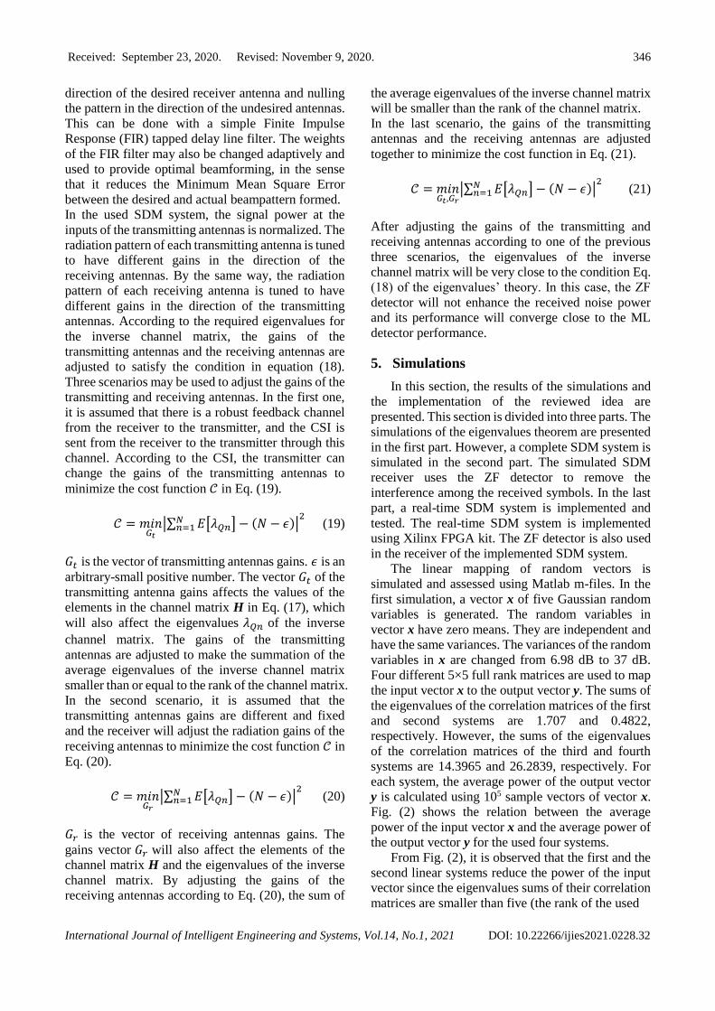
Fig. (2) shows the relation between the average
power of the input vector x and the average power of
the output vector y for the used four systems.
From Fig. (2), it is observed that the first and the
second linear systems reduce the power of the input
vector since the eigenvalues sums of their correlation
matrices are smaller than five (the rank of the used

Received: September 23, 2020. Revised: November 9, 2020. 347
International Journal of Intelligent Engineering and Systems, Vol.14, No.1, 2021 DOI: 10.22266/ijies2021.0228.32
Figure. 2 The input/output average power relation for four linear systems with different correlation matrices
linear systems). However, the third and the fourth
linear systems increase the power of the input vector
since the eigenvalues sums of their correlation
matrices are greater than five. This observation
confirms the contribution of the eigenvalues’
theorem. According to Eq. (10), the power gain of the
linear system is equal to the trace of its correlation
matrix divided by its rank. The power gains of the
first and second systems are -4.6674 dB and -10.1571
dB, respectively. On the other hand, the power gains
of the third and fourth systems are 4.5929 dB and
7.2072 dB, respectively.
In the next simulation, the performance of a
random linear system is evaluated. Two different
input vectors x1 and x2 are used in this simulation.
Each vector consists of five independent Gaussian
random variables with zero means. The average
power of x1 is 0 dB and the average power of x2 is 10
dB. The random system is a 5×5 zero-mean Rayleigh
random matrix (A). 105 different input vectors of x1
and x2 are used in the simulation. The system matrix
A is randomly changed with each input vector. There
are 105 random Rayleigh matrices affect the elements
of the input vectors at each time the simulation is
done. The vectors y1 and y2 are the output vectors
from the random system A due to the input vector x1
and x2, respectively. The average powers of y1 and y2
are calculated for each input of x1 and x2. According
to the eigenvalues’ theorem and Eqs. (11) and (14),
the average eigenvalue (AEV) of the five random
eigenvalues of the correlation matrix 𝐸[𝐀 𝐀𝐻] is
calculated. Moreover, the sum of the five average
eigenvalues (SAEVs) of the correlation matrix
𝐸[𝐀 𝐀𝐻] is calculated at each time the simulation is
done. The previous simulation and calculations are
repeated 30 times. In each time, the variances of the
elements of matrix A are changed to have different
values of the AEV of the correlation matrix 𝐸[𝐀 𝐀𝐻]. The 105 Rayleigh random matrices, which affect the
input vectors, are also changed each time the
simulation is repeated. Fig. 3 shows the relation
between the SAEVs of the correlation matrix
𝐸[𝐀 𝐀𝐻] versus its AEV. The average power of the
output vectors from the random system A is
calculated and displayed in Fig. 3. According to Eq.
(14), the rank threshold of the sum of the eigenvalues
averages of the correlation matrix 𝐸[𝐀 𝐀𝐻] is 6.9897
dB. It is also shown in Fig. 3.
In Fig. 3, the threshold boundary is specified. It is
the vertical line at the intersection point between the
rank threshold line and the line of the SAEVs of the
correlation matrix 𝐸[𝐀 𝐀𝐻]. It is observed that the
average power of the output vectors from the random
system A on the left-hand side of the threshold
boundary is smaller than the average power of the
input vectors. However, on the right-hand side of the
boundary, the average power of the output vectors is
greater than the average power of the input vectors.
In other words, the average power of the output
vector from the random system A is smaller than the
average power of its input vector as long as the
SAEVs of the correlation matrix 𝐸[𝐀 𝐀𝐻] is smaller
than the rank threshold (6.9897 dB), and vice versa.
This observation confirms the contribution of the
eigenvalues’ theorem. In the last simulation of this
part, the performance of the ZF detector is evaluated
individually with noise vectors. In the ZF detector,
the linear mapping is done using the inverse of the
channel matrix. Since the channel matrix is often a
Rayleigh matrix, the linear mapping in the ZF
detector is done using the inverse of a Rayleigh
matrix.
The parameters of the previous simulations are
repeated in this simulation except that the mapping
process is done using the inverse matrix A-1. The
average powers of the output vectors and the SAEVs
of the correlation matrix 𝐸[𝐀−1(𝐀−1)𝐻] are
calculated and represented in Fig. 4. The calculated
5 10 15 20 25 30 35 40
Average power of input vector (dB)
-10
0
10
20
30
40
50
Ave
rag
e p
ow
er
of o
utp
ut
vecto
r (d
B) Linear system 1
Linear system 2
Linear system 3
Linear system 4

Received: September 23, 2020. Revised: November 9, 2020. 348
International Journal of Intelligent Engineering and Systems, Vol.14, No.1, 2021 DOI: 10.22266/ijies2021.0228.32
Figure. 3 The input/output average power relation for a random linear system with two different input vectors x1 and x2
Figure. 4 The input/output average power relation for the ZF detector with two different input vectors x1 and x2
parameters are shown versus the AEV of the
correlation matrix 𝐸[𝐀𝐀𝐻]. From Fig. 4, it is observed that the average output
powers and the SAEVs of the correlation matrix
𝐸[𝐀−1(𝐀−1)𝐻] are inversely proportional with the
AEV of the channel correlation matrix 𝐸[𝐀𝐀𝐻]. This
is opposite of what happened in the previous
simulation because the mapping process in the ZF
detector is done using the inverse of the random
Rayleigh matrix A. The threshold boundary is also
specified in Fig. 4. It is observed that the average
power of the output vectors from the ZF detector on
the right-hand side of the threshold boundary is
smaller than the average power of its input vectors.
However, on the left-hand side of the boundary, the
average power of the output vectors is greater than
the average power of the input vectors. Hence, the
average power of the output of ZF detector is smaller
than the average power of its input as long as the
SAEVs of the correlation matrix 𝐸[𝐀−1(𝐀−1)𝐻] is
smaller than the rank threshold (6.9897 dB), and vice
versa.
From Fig. 4, a very important conclusion is noted.
As long as the AEV of the correlation matrix 𝐸[𝐀𝐀𝐻]
of the used Rayleigh matrix is greater than 17.6 dB,
the ZF detector will not increase the power of the
input noise vector. This conclusion does not depend
on the power of the noise vector. It depends only on
the eigenvalues of the correlation matrix 𝐸[𝐀𝐀𝐻] .
The AEV of the correlation matrix of the Rayleigh
channel in real communications systems is always
less than the AEV of the rank threshold boundary.
This is the reason behind the bad impression of the
ZF detector performance. To get benefits from the
previous contribution, the channel parameters, which
merely affects the desired signal, should be changed
to increase the AEV of the channel correlation matrix.
For example, the gains of the transmitting antennas
or the receiving antennas are adjusted to make the
AEV of the correlation matrix of the Rayleigh
channel greater than the AEV of the threshold
boundary. Table 1 lists the estimations of the AEV of
the threshold boundary for different Rayleigh
channel matrices with different ranks.
The values of the AEV in Table 1 are determined
from the simulations with an estimation error around
±1 dB. They may be used as a rough guide in
designing SDM systems with ZF detectors. For
-2 -1.5 -1 -0.5 0 0.5 1 1.5 2 2.5 3 3.5 4 4.5 5
AEV of the random correlation matrix E[A.AH
] (dB)
-20
-15
-10
-5
0
5
10
15
20
25
30
Pow
er
(dB
)
The rank of the system
SAEVs of the correlation matrix E[A.AH
]
Output power of y1
Output power of y2
Input power of x1
Input power of x2
Threshold Boundary
5 10 15 20 25 30 35
AEV of the channel correlation matrices E[A.AH
](dB)
-20
-15
-10
-5
0
5
10
15
20
25
30
Po
we
r (d
B)
The rank of the system
SAEVs of the correlation matrix E[A-1
.(A-1
)H
]
Output power of y1
Output power of y2
Input power of x1
Input power of x2
Threshold Boundary

Received: September 23, 2020. Revised: November 9, 2020. 349
International Journal of Intelligent Engineering and Systems, Vol.14, No.1, 2021 DOI: 10.22266/ijies2021.0228.32
Table 1. The estimations of the AEV of the threshold
boundary for rayleigh channel correlation matrix at
different matrix ranks
The rank of Rayleigh
channel matrix
The average eigenvalue of the
threshold boundary
2 13 dB
3 15.1 dB
4 16.2 dB
5 17.6 dB
6 18.5 dB
7 19 dB
8 19.3 dB
Table 2. The AEV of the correlation matrices of the
simulated rayleigh channels and the SAEVs of the
correlation matrices of their inverse
Channel
matrix
The AEV of the
channel correlation
matrix
The SAEVs of the
inverse channel
correlation matrix
Group 1 4 dB 18.87 dB
Group 2 17 dB 6.13 dB
Group 3 30 dB -7.42 dB
accurate calculations of the AEV values, the
probability density function (pdf) of the eigenvalues
of the channel correlation matrix 𝐸[𝐀𝐀𝐻] and the pdf
of the SAEVs of the correlation matrix
𝐸[𝐀−1(𝐀−1)𝐻] need to be determined. This is not an
easy task. This problem may be studied in detail in
aseparate work to reduce prolongation in this article.
In the second part of the simulations, the
performance of an SDM receiver with ZF detector is
evaluated. The simulated SDM system uses 4
transmitting antennas and 4 receiving antennas. The
used modulation scheme is 16-QAM (Quadrature
Amplitude Modulation). The coherence bandwidth of
the Rayleigh channel is 6 MHz. The bandwidth of the
transmitted signal is 5 MHz. The transmission bit rate
in the simulated SDM system is 40 Mbit/s. However,
the transmission bit rate in the corresponding non-
multiplexing system is 10 Mbit/s. The receiver uses a
ZF detector to remove interference among the
received symbols. The AEV of the channel
correlation matrix and the SAEVs of the inverse
channel correlation matrix are calculated. The AEV
Figure. 5 The BER performance of SDM receiver with ZF detector at different matrices of rayleigh flat fading channels
Figure. 6 A comparison between the SNR before and after ZF detector in SDM receiver at different matrices of rayleigh
flat fading channels
10 15 20 25 30 35 40
Average SNR (dB)
10-6
10-5
10-4
10-3
10-2
10-1
100
Ave
rage
Bit E
rror
Ra
te
AEV= 4 dB, SAEVs=18.87 dB
AEV= 17 dB, SAEVs=6.13 dB
AEV= 30 dB, SAEVs=-7.42 dB
Theoretical Pe in Rayleigh flat fading channel
-5 0 5 10 15 20 25 30
Average SNR before ZF detector (dB)
-20
-10
0
10
20
30
40
50
Ave
rag
e S
NR
aft
er
ZF
de
tecto
r (d
B)
AEV= 4 dB, SAEVs=18.87 dB
AEV= 17 dB, SAEVs=6.13 dB
AEV= 30 dB, SAEVs=-7.42 dB

Received: September 23, 2020. Revised: November 9, 2020. 350
International Journal of Intelligent Engineering and Systems, Vol.14, No.1, 2021 DOI: 10.22266/ijies2021.0228.32
represents the average power gain of the channel.
However, the SAEVs of the inverse channel
correlation matrix divided by the rank of the channel
matrix (N) represents the total power gain of the ZF
detector. According to the used channel model, the
channel matrix changes randomly every symbol
period Ts. Table 2 shows the values of AEV and
SAEVs for three different groups of channels
matrices.
The simulation is repeated three times for the
three different channels groups in Table 2. The signal
to interference ratio (SIR) at each receiving antenna
is -4.77 dB. SIR is the ratio between signal power and
interference power. The average received SNR is
changed from 10 dB to 40 dB. SNR is the ratio
between signal power and noise power. Fig. 5 shows
the Bit-Error-Rate (BER) performance of the
simulated SDM system at each value of the average
received SNR. The BER is the ratio between the
number of bit errors in the received data and the total
number of received bits. The calculated BER is
compared with the theoretical probability of error of
the 16-QAM system in Rayleigh flat fading channel.
According to the introduced eigenvalues theorems,
the rank of the channel matrix is 6 dB.
From Fig. 5, it is observed that the optimum
performance of the simulated SDM receiver is
achieved when the SAEVs of the inverse channel
correlation matrix is equal to the rank of the channel
matrix (6 dB). In this case, the total average power
gain of the ZF detector is approximately 0 dB. This
happens with the second group of channel matrices,
at which the average power gain of the channel is
approximately 17 dB. Since the real flat fading
channel is passive, the channel gain is achieved in
real systems by increasing the power amplifiers gains
in the transmitter or changing the gains of the
transmitting antennas and the receiving antennas.
When the average channel gain increases more
than 17 dB, the BER performance of the ZF detector
is enhanced because the SAEVs of the inverse
channel correlation matrix is smaller than the rank of
the channel matrix. This enhancement does not
depend on the received SNR. This is observed in the
simulation with the third group of channels. The
Figure. 7 The BER performance of the SDM receiver with ZF detector versus the received SNIR at different matrices
of rayleigh flat fading channels
Figure. 8 A comparison between the SNIR before ZF detector and SNR after ZF detector in SDM receiver at different
matrices of rayleigh flat fading channels
10 15 20 25 30 35 40
Average SNIR (dB)
10-6
10-5
10-4
10-3
10-2
10-1
100
Ave
rage
Bit E
rro
r R
ate
AEV= 4 dB, SAEVs=18.81 dB
AEV= 17 dB, SAEVs=6.06 dB
AEV= 30 dB, SAEVs=-6.76 dB
Theoretical Pe in Rayleigh flat fading channel
-5 0 5 10 15 20 25 30
Average SNIR before ZF detector (dB)
-20
0
20
40
60
80
Ave
rag
e S
NR
aft
er
ZF
de
tecto
r (d
B)
AEV= 4 dB, SAEVs=18.81 dB
AEV= 17 dB, SAEVs=6.06 dB
AEV= 30 dB, SAEVs=-6.76 dB

Received: September 23, 2020. Revised: November 9, 2020. 351
International Journal of Intelligent Engineering and Systems, Vol.14, No.1, 2021 DOI: 10.22266/ijies2021.0228.32
Table 3. Synthesis results of the implemented SDM system
Resource Available Transmitter Receiver Utilization %
LUT 303600 55324 125179 59.45
FF 607200 82331 180844 43.34
IO 700 24 24 6.8
BUFG 32 5 7 37.5
Worst negative slack 0.832 ns 0.087 ns
Worst hold slack 0.042 ns 0.035 ns
SAEVs is approximately 13.5 dB lower than the rank
threshold. The BER performance of the SDM system
with the third channel group is 13 dB better than the
theoretical probability of error of 16-QAM systems,
whatever the received SNR is.
This performance enhancement is not due to the
increase in the received SNR since the BER is
calculated at the same values of the SNRs used with
the second group of channels. However, the
performance enhancement is due to that the ZF
detector will reduce noise power at its output to be
smaller than the noise power at its input when the
SAEVs is smaller than the rank.
Finally, when the first group of the channel matrix is
used in the simulation, it gives the worst BER
Figure. 9 The BER performance of real-time SDM system with ZF detector versus the received SNIR at different
matrices of rayleigh flat fading channels
Figure. 10 A comparison between the SNIR before ZF detector and SNR after ZF detector in real-time SDM receiver at
different matrices of rayleigh flat fading channel
10 15 20 25 30 35 40Average SNIR (dB)
10-5
10-4
10-3
10-2
10-1
Ave
rag
e B
it E
rro
r R
ate
AEV= 10.78 dB, SAEVs=10.12 dB
AEV= 20.78 dB, SAEVs=-0.612 dB
Theoretical Pe in Rayleigh flat fading channel
0 5 10 15 20 25 30
Average SNIR before ZF detector (dB)
10
20
30
40
50
60
70
Ave
rag
e S
NR
aft
er
ZF
de
tecto
r (d
B)
AEV= 10.78 dB, SAEVs=10.12 dB
AEV= 20.78 dB, SAEVs=-0.612 dB

Received: September 23, 2020. Revised: November 9, 2020. 352
International Journal of Intelligent Engineering and Systems, Vol.14, No.1, 2021 DOI: 10.22266/ijies2021.0228.32
performance because the SAEVs is bigger than the
rank threshold of the channel matrix. In this case, the
ZF detector enhances the noise power at its outputs.
The SNR at the input of the baseband detector is
smaller than the SNR at the input of the baseband
detector of the previous two cases. This is the reason
for the bad BER performance of the ZF detector when
the first group of the channel matrix is used.
Fig. 6 displays the average SNR at the output of the
ZF detector versus the average SNR at its input for
the previous three channels groups. The figure
confirms the aforementioned contributions. The
average SNR at the output of the ZF detector changes
for the same SNR at its input according to the used
channel group. The average SNR at the output of the
ZF detector is bigger than the average SNR at its
input as long as the SAEVs of the inverse channel
correlation matrix is smaller than the rank threshold.
This is the reason why the BER performance is better
in the case of the third channel group than the other
cases.
The previous simulation is repeated but the
average BER is displayed versus the average received
Signal to Noise and Interference Ratio (SNIR) at each
receiving antenna. Fig. 7 shows the average BER
versus the average SNIR and Fig. 8 shows the
average SNR at the output of the ZF detector versus
the average SNIR at its input. The same observations
are contributions are achieved for this simulation.
Therefore, the BER performance of the ZF
detector neither depends on the received noise power
nor the received interference power, but it depends on
the eigenvalues of the correlation matrix of the
inverse channel matrix.
In the last part of this section, a real-time
implementation of the simulated SDM system is
tested with a practical Rayleigh channel. Xilinx
FPGA kit is used to implement the SDM transmitter
and receiver. The used FPGA platform is Virtex-7
VC707. Table 2. lists the synthesis results of the
implemented SDM system.
A file of 1 G bits is transmitted with a rate of 30
M bits/s. The carrier frequency of the transmitted
signal is 5 GHz. 3 transmitting antennas and 3
receiving antennas are used in the implemented
system. The spacing between the antennas is 30 cm.
According to the eigenvalues’ theorems, the rank
threshold of the channel matrix is 4.77 dB. From
Table 2, the average channel gain should be greater
than 15.1 dB to use ZF detector in the receiver
without any noise enhancement. The power
amplifiers and the gains of the transmitting antennas
and receiving antennas are considered as a part of the
channel matrix. The gains of the power amplifiers,
the transmitting antennas, and receiving antennas are
adjusted to get two different channel matrices with
AEV of 10.78 dB and 20.78 dB. The received average
SNIR is changed from 20 dB to 35 dB. The average
BER is calculated and displayed in Fig. 9 using the
previous two channels.
Form Fig. 9, it is observed that the average BER
is changed for the same received SNIR according to
the value of the AEV of the channel matrix. When the
AEV is bigger than 15.1 dB, the average BER is
smaller than the BER when the AEV is smaller
than15.1 dB. The SAEVs in the second case is
smaller than the rank threshold of 4.77 dB. However,
the SAEVs in the first case is bigger than the rank
threshold.
Therefore, the performance of the ZF detector is
not affected with the received SNIR but it is affected
with the AEV of the channel correlation matrix and
the SAEVs of the inverse channel correlation matrix.
The AEV of the channel correlation matrix can be
controlled by the power amplifiers gains in the
transmitter, the gains of the transmitting antennas and
the gains of the receiving antennas. Fig. 10 display
the average SNR at the output of the ZF detector
versus the average SNIR at its input. The average
SNR at the output of the ZF detector is smaller than
the Average SNR at its input as long as the SAEVs of
the correlation matrix of the ZF detector mapping
matrix is smaller than the rank threshold, and vice
versa.
6. Conclusions
SDM system increases the data transmission rate
by sending the modulated symbols parallel using
different transmitting antennas. SDM system sends
the modulated symbols in the same bandwidth, which
is used by the non-multiplexing system. The
bandwidth efficiency of the SDM system is greater
than the bandwidth efficiency of any other
multiplexing system. The channel model of the SDM
system is conserved as a flat fading channel to
prevent ISI among the received symbols. This is
accomplished by reducing the transmission rate of
each transmitting antenna to get a transmission
bandwidth smaller than the coherence bandwidth of
the channel. In the same time, the number of the
transmitting antennas is increased to achieve the
required high transmission rate.
In the used SDM receiver, ZF detector is used
after the matched filters to remove interferences
among the multiplexed symbols because its
complexity changes linearly with the number of the
interfering symbols. The random variables in the
noise vector after the matched filters in the SDM
receiver are independent and have the same
Received: September 23, 2020. Revised: November 9, 2020. 353
International Journal of Intelligent Engineering and Systems, Vol.14, No.1, 2021 DOI: 10.22266/ijies2021.0228.32
probability distribution functions. The noise
performance of the ZF detector does not depend on
the received SNR. The eigenvalues of the correlation
matrix of the ZF detector-mapping matrix and the
rank of this mapping matrix are the parameters,
which control the performance of the ZF detector.
The channel noise power at the outputs of the ZF
detector increases or decreases according to the
relation between the sum of the eigenvalues of the
correlation matrix of the ZF detector and the rank of
its mapping matrix. If the sum of these eigenvalues is
greater than the rank of the mapping matrix, the ZF
detector will enhance the channel noise power at its
output and the BER will increase at the output of the
baseband detector. However, if the sum of these
eigenvalues is equal to the mapping matrix rank, the
ZF detector will not enhance the noise power at its
output and the BER performance of the ZF detector
will be closed to the BER performance of the ML
detector. Moreover, the ZF detector will reduce the
channel noise power at its output if the sum of these
eigenvalues is smaller than the mapping matrix rank.
Since the mapping matrix of the ZF detector is the
inverse of the channel matrix, there is a relation
between the average eigenvalue of the channel
correlation matrix and the sum of the eigenvalues of
the correlation matrix of the ZF detector-mapping
matrix. Simulation results show that the ZF detector
will not increase the noise power at its outputs if the
average eigenvalue of the channel correlation matrix
is greater than a certain threshold. The results of the
simulations give estimations for this threshold for
different ranks of channel matrices. According to the
used mathematical model, the elements of the
channel matrix depend on the transmitting antennas
gains and the receiving antennas gains. By adjusting
these gains, the average eigenvalue of the channel
matrix can be greater than the estimated threshold. In
this case, the ZF detector reduces the power of the
channel noise whatever its input SNR is high or low.
The noise performance of the ZF detector does not
depend on the received SNR, but it depends on the
average eigenvalue of the channel correlation matrix.
The output SNR at the output of the ZF detectors
changes according to the average eigenvalue of the
correlation matrix at the same input SNR.
In future work, the probability distribution of the
average eigenvalue of the channel correlation matrix
and the probability distribution of the sum of the
eigenvalues of the ZF detector correlation matrix will
be determined. A mathematical equation, which
gives the estimation of the average eigenvalue
threshold of the channel matrix, will also be specified.
Declaration of interests
The authors declare no conflict of interest.
Author Contributions
“Conceptualization, A. Y. Hassan; methodology,
A. Y. Hassan; software, A. Y. Hassan and Ali Saleh;
validation, A. Y. Hassan and Ali Saleh; formal
analysis, A. Y. Hassan; investigation, A. Y. Hassan
and Ali Saleh; resources, A. Y. Hassan; data curation,
Ali Saleh; writing—original draft preparation, A. Y.
Hassan —review and editing, A. Y. Hassan and Ali
Saleh; visualization, A. Y. Hassan; supervision, A. Y.
Hassan; project administration, A. Y. Hassan;
funding acquisition, A. Y. Hassan.
References
[1] J. Choi, Y. Nam, and N. Lee, “Spatial Lattice
Modulation for MIMO Systems”, IEEE
Transactions on Signal Processing, Vol. 66, No.
12, pp. 3185-3198, 2018.
[2] S. Gao, X. Cheng, and L. Yang, “Spatial
Multiplexing with Limited RF Chains:
Generalized Beamspace Modulation (GBM) for
mmWave Massive MIMO”, IEEE Journal on
Selected Areas in Communications, Vol. 37, No.
9, pp. 2029-2039, 2019.
[3] X. Liu and I. Darwazeh, “Doubling the Rate of
Spectrally Efficient FDM Systems Using Hilbert
Pulse Pairs”, In: Proc. of 26th International Conf.
on Telecommunications (ICT), Hanoi, Vietnam,
pp. 192-196, 2019.
[4] U. Choudhary and V. Janyani, “Bandwidth
efficient frame structures for flip OFDM with
phase conjugated sub carriers and LDPC
encoding”, Optik, Vol. 204, 2020.
[5] Z. Wang, L. Zheng, J. Chen, M. Lin, and X.
Deng, “MIMO-MFSK Spatial Multiplexing in
Rician Channel with Large Doppler Shift”, In:
Proc. of IEEE 19th International Conf. on
Communication Technology (ICCT), Xi'an,
China, pp. 649-652, 2019.
[6] A. Udawat and S. Katiyal, “Signal detection
techniques for spatially multiplexed MIMO
systems”, In: Proc. of 6th International Conf. on
Computing for Sustainable Global Development,
New Delhi, India, p 432-434, 2019.
[7] T. S. Rappaport, Wireless Communications:
Principles and Practice, Prentice Hall, 2nd
edition, 2002.
[8] A. Y. Hassan, “Minimizing the Effects of Inter-
Carrier Interference Signal in OFDM System
Using FT-MLE Based Algorithm”, Wireless

Received: September 23, 2020. Revised: November 9, 2020. 354
International Journal of Intelligent Engineering and Systems, Vol.14, No.1, 2021 DOI: 10.22266/ijies2021.0228.32
Personal Communications, Springer, Vol. 97,
No. 2, pp 1997–2015, 2017.
[9] A. Y. Hassan, “A Novel Structure of High Speed
OFDM Receiver to Overcome ISI and ICI in
Rayleigh Fading Channel”, Wireless Personal
Communications, Springer, Vol. 97, No. 3, pp
4305–4325, 2017.
[10] S. Birgmeier and N. Goertz, “Approximate
Message Passing for Joint Activity Detection
and Decoding in Non-orthogonal CDMA”, In:
Proc. of 23rd International ITG Workshop on
Smart Antennas, Vienna, Austria, pp. 1-5, 2019.
[11] Y. Liu, W. Zhang, and P. C. Ching, “Time-
reversal space–time codes in asynchronous two-
way relay networks”, IEEE Transactions on
Wireless Communication, Vol. 15, No. 3, pp.
1729-1741, 2016.
[12] W. Tang, S. Yang, and X. Li, “Implementation
of Space-time Coding and Decoding Algorithms
for MIMO Communication System Based on
DSP and FPGA”, In: Proc. of IEEE
International Conf. on Signal Processing,
Communications and Computing (ICSPCC),
Dalian, China, pp. 1-5, 2019.
[13] I. Ahn, J. Kim, and H. Song, “Adaptive Analog
Self-Interference Cancellation for In-band Full-
Duplex Wireless Communication”, In: Proc. of
IEEE Asia-Pacific Microwave Conf. (APMC),
Marina Bay Sands, Singapore, pp. 414-416,
2019.
[14] P. Herath, A. Haghighat, and L. Canonne-
Velasquez, “A Low-Complexity Interference
Cancellation Approach for NOMA”, In: Proc. of
IEEE 91st Vehicular Technology Conf.
(VTC2020-Spring), Antwerp, Belgium, pp. 1-5,
2020.
[15] M. Gao, L. Zhang, C. Han, and J. Ge, “Low-
Complexity Detection Schemes for QOSTBC
with Four-Transmit-Antenna”, IEEE
Communications Letters, Vol. 19, No. 6, pp.
1053-1056, 2015.
[16] S. Verdu, “Multiuser Detection”, Cambridge
press, U.K, 1998.
[17] Y. Hama and H. Ochiai, “A low-complexity
matched filter detector with parallel interference
cancellation for massive MIMO systems”, In:
Proc. of IEEE 12th International Conf. on
Wireless and Mobile Computing, Networking
and Communications (WiMob), New York,
United State, pp. 1-6, 2016.
[18] J. GuEmaila and R. Lamare, “Joint interference
cancellation and relay selection algorithms
based on greedy techniques for cooperative DS-
CDMA systems”, EURASIP Journal on
Wireless Communications and Networking, Vol.
59, pp. 1-19, 2016.
[19] L. Fang, L. Xu, and D. Huang, “Low
Complexity Iterative MMSE-PIC Detection for
Medium-Size Massive MIMO”, IEEE Wireless
Communications Letters, Vol. 5, No. 1, pp. 108-
111, 2016.
[20] B. Ling, C. Dong, J. Dai, and J. Lin, “Multiple
Decision Aided Successive Interference
Cancellation Receiver for NOMA Systems”,
IEEE Wireless Communications Letters, Vol. 6,
No. 4, pp. 498-501, 2017.
[21] F. Uddin and S. Mahmud, “Carrier Sensing-
Based Medium Access Control Protocol for
WLANs Exploiting Successive Interference
Cancellation”, IEEE Transactions on Wireless
Communications, Vol. 16, No. 6, pp. 4120-4135,
2017.
[22] M. Mandloi, M. Hussain, and V. Bhatia,
“Improved multiple feedback successive
interference cancellation algorithms for near-
optimal MIMO detection”, IET
Communications, Vol. 11, No. 1, pp. 150-
159,2017.
[23] R. Fischer, C. Stierstorfer, and R. Mueller,
“Subspace Projection and Noncoherent
Equalization in Multi-User Massive MIMO
Systems”, In: Proc. of 10th International ITG
Conf. on Systems, Communications and Coding,
Hamburg, Germany, pp. 1-6, 2015
[24] S. Şahin, A. M. Cipriano, C. Poulliat, and M.
Boucheret, “Iterative Equalization with
Decision Feedback Based on Expectation
Propagation”, IEEE Transactions on
Communications, Vol. 66, No. 10, pp. 4473-
4487, 2018.
[25] C. Dong, K. Niu, and J. Lin, “An Ordered
Successive Interference Cancellation Detector
with Soft Detection Feedback in IDMA
Transmission”, IEEE Access, Vol. 6, pp. 8161-
8172, 2018.
[26] J. Minango, C. Altamirano, and C. Almeida,
“Performance difference between zero-forcing
and maximum likelihood detectors in massive
MIMO systems”, Electronics Letters, Vol. 54,
No. 25, pp. 1464-1466, 2018.
[27] S. Hu and E. Leitinger, “Joint Modulus Zero-
Forcing MIMO Detector”, In: Proc. of IEEE
Wireless Communications and Networking Conf.
(WCNC), Marrakesh, Morocco, pp. 1-5, 2019.
[28] J.G. Proakis, Digital communications, New
York: McGraw-Hill, 2001.
[29] Y. Khattabi and M. Matalgah, “Improved error
performance ZFSTD for high mobility relay-

Received: September 23, 2020. Revised: November 9, 2020. 355
International Journal of Intelligent Engineering and Systems, Vol.14, No.1, 2021 DOI: 10.22266/ijies2021.0228.32
based cooperative systems”, Electronics Letters,
Vol. 52, No. 4, pp. 323-325, 2016
[30] H. Q. Ngo, M. Matthaiou, T. Q. Duong, and E.
G. Larsson, “Uplink Performance Analysis of
Multicell MU-SIMO Systems with ZF
Receivers”, IEEE Transactions on Vehicular
Technology, Vol. 62, No. 9, pp. 4471-4483,
2013.
[31] E. Guerrero, G. Tello, and F. Yang, “Simulation
and performance analysis for ordering algorithm
in ZF and MMSE detectors for V-BLAST
architectures”, In: Proc. of International Conf.
on Computer Science and Network Technology,
Harbin, United State, pp. 59-64, 2011.