Embed Size (px)
Citation preview

DI
SC
US
SI
ON
P
AP
ER
S
ER
IE
S
Forschungsinstitut zur Zukunft der ArbeitInstitute for the Study of Labor
The Effect of Family Disruption on Children’sPersonality Development: Evidence fromBritish Longitudinal Data
IZA DP No. 8712
December 2014
Tyas PrevooBas ter Weel
The Effect of Family Disruption on
Children’s Personality Development: Evidence from British Longitudinal Data
Tyas Prevoo Maastricht University
Bas ter Weel
CPB Netherlands Bureau for Economic Policy Analysis, Maastricht University and IZA
Discussion Paper No. 8712 December 2014
IZA
P.O. Box 7240 53072 Bonn
Germany
Phone: +49-228-3894-0 Fax: +49-228-3894-180
E-mail: [email protected]
Any opinions expressed here are those of the author(s) and not those of IZA. Research published in this series may include views on policy, but the institute itself takes no institutional policy positions. The IZA research network is committed to the IZA Guiding Principles of Research Integrity. The Institute for the Study of Labor (IZA) in Bonn is a local and virtual international research center and a place of communication between science, politics and business. IZA is an independent nonprofit organization supported by Deutsche Post Foundation. The center is associated with the University of Bonn and offers a stimulating research environment through its international network, workshops and conferences, data service, project support, research visits and doctoral program. IZA engages in (i) original and internationally competitive research in all fields of labor economics, (ii) development of policy concepts, and (iii) dissemination of research results and concepts to the interested public. IZA Discussion Papers often represent preliminary work and are circulated to encourage discussion. Citation of such a paper should account for its provisional character. A revised version may be available directly from the author.
IZA Discussion Paper No. 8712 December 2014
ABSTRACT
The Effect of Family Disruption on Children’s Personality Development: Evidence from British Longitudinal Data*
This research documents the effects of different forms of family disruptions – measured by separation, divorce and death – on personality development of British children included in the 1970 British Cohort Study. There are statistically significant correlations between family disruptions prior to the age of 16 and personality development in early childhood. Parental divorce has the largest negative effect on a child’s personality development. Family disruptions have smaller effects on personality development when children are older and patterns differ by gender. The relationship between personality development and family disruption is partially driven by selection. Placebo regressions reveal significant correlations between family disruption and personality development before disruption. The omitted variable bias is mitigated by investigating mechanisms through which the selection operates. JEL Classification: J12, J24 Keywords: family disruption, personality development Corresponding author: Bas ter Weel CPB Board of Directors PO Box 80510 2508 GM Den Haag The Netherlands E-mail: [email protected]
* We would like to thank the editor and two referees of this journal for helpful feedback. In addition, Lex Borghans, Nicole Bosch, and Suzanne Kok have provided insightful comments on an earlier draft of this paper.
1 Introduction
A growing body of literature in economics and psychology has shown that personality traits are im-
portant predictors of a variety of socioeconomic outcomes (e.g. Almlund, Duckworth, Heckman &
Kautz, 2011; Borghans, Duckworth, Heckman & Ter Weel, 2008, for overviews). The development
of personality traits seems to be strongly influenced by the stability of the family environment chil-
dren experience (e.g. Knudsen, Heckman, Cameron & Shonkoff, 2006). Early life experiences, such
as disruptions in family structure, could act as an impediment to a child’s personality development.
This paper empirically analyses the effect of family disruptions on children’s personality develop-
ment. We focus on disruptions that involve the breakdown of the two-parent family into a family
in which only one natural parent is left. We do so by documenting and interpreting personality
development of the children included in the 1970 British Cohort Study (BCS). The BCS is a lon-
gitudinal survey including all children born in Britain in the week of 5-11 April 1970. The setup
of our empirical analysis is divided into three steps. First, a set of descriptive analyses provides
insight into the changes that children go through in terms of the mean-level development of per-
sonality traits when they are confronted with family disruption. We compare these developments
with children who grow up in intact families. Second, we focus on heterogeneity in personality
development across children by investigating to what extent the experience of family disruption
explains intra-individual differences from early to late childhood. In particular, we analyse different
types of family disruption, the age at which the child experiences the disruption, and differences
in personality development between boys and girls. Finally, while life experiences are generally
found to be correlated with personality changes, the endogenous nature of the occurrence of these
experiences is generally ignored. We address this issue by running placebo tests and by dealing
with sample selection in the BCS.
In this paper we measure personality by three traits: self-esteem, internal locus of control and
behavioural problems. In psychology these measures are often used to measure personality de-
velopment in children (Almlund et al., 2011) and economists have applied them in their research
to measure personality development and behavioural problems in children (e.g. Currie & Stabile,
2006). Our analyses show that children mature in terms of personality during childhood, but that
this development is significantly affected by family disruptions. Between the ages of 10 and 16,
children generally demonstrate positive personality development, as shown by increasing scores
on self-esteem and internal locus of control, as well as decreasing scores on the Rutter index for
behavioural problems. These favourable changes are significantly smaller for children who have
experienced family disruptions. Family disruption has both a level and growth effect on personality
development. Children who do not live with both natural parents throughout childhood not only
rank lower in terms of personality traits at the age of 16, but also show less growth between the
ages of 10 and 16.1
1Losing one of two natural parents in the household does not necessarily imply that the lost parent is absent
all of the time. Next to changes as a result of death, separation or divorce of parents could mean that the role
of the lost parent in the child’s life has changed. In all cases, the lost parents could have been replaced with a
stepparent of other mother/father figure. These influences are not taken into consideration in this study because we
2
While regression analyses demonstrate that family disruption is associated with a quarter of a
standard deviation lower levels of favourable personality traits, the correlations drop when controls
for the quality of the home environment are added to the regression models. Schooling and social
class of parents are significantly related to the personality traits of their children. Yet, they do
not affect the association between family disruption and personality development in a strong way.
Variables related to closeness of the parent-child relationship mediate the relationship between
family disruption and personality development. To adjust for these confounding factors, and the
possible endogeneity of family composition, a more elaborate set of covariates - including birth
conditions, social class, and family characteristics - is included in all analyses.
The reason for family disruption, the age at which this occurs, and the gender of the child matter for
the size of the estimated coefficient. While children seem to recover from experiencing the death of
a parent in terms of personality outcomes, children from divorced parents show significantly lower
self-esteem and internal locus of control, while also scoring higher on the behavioural problems
index. Further, the effects of family disruption seem to be less pronounced if the child was older
at the time of the disruption. In terms of an overall effect of family disruption on personality
development, there seem to be no overall differences between boys and girls. However, boys seem
to suffer more from the death of a parent relative to girls, while the effect of experiencing divorce
of parents is more severe for girls’ personality development.
Family disruptions are to some extent endogenous. Families that break down are different from
families that remain intact, even before the observed change. This is demonstrated by reductions
in the estimated effect size, once additional controls for the quality of the home environment are
added to the models. Key components are mother’s age at birth of the child, parental education,
family income, and parental care. We attempt to deal with possible endogeneity of our estimation
results by presenting different sets of estimates for parental death and divorce, where we assume
the former to be exogenous.
The analyses presented in this study contribute to the literature on the development of personality
traits during childhood. The development of personality can be measured in various ways. Using
meta-analytic techniques, Roberts, Walton & Viechtbauer (2006) show the pattern of mean-level
changes in terms of Big Five personality traits and observe that the largest changes occur early in
life. Measuring personality development in terms of rank-order stability, by reporting correlations
between personality scores across two points in time, reflects the degree to which the relative
ordering of individuals is maintained. These changes in rank-order development are also largest
early in life (Roberts & DelVecchio, 2000). Theories on personality trait development attribute
personality changes to a combination of environmental and genetic factors, as well as life experiences
(see Roberts et al., 2006, for a discussion).
Empirical studies investigating the association between life experiences and personality change
seem to be inconclusive. For working-age adults, Cobb-Clark & Schurer (2012) show that mean-
level changes are small and intra-individual changes are generally unrelated to adverse employment,
lack information in our data.
3
health and family-related events. Specht, Schmukle & Egloff (2011), however, conclude that such
events do explain a significant part of the variation in personality traits. They also show that
when events are clustered, as in Cobb-Clark & Schurer (2012), effects of the environment may
be overlooked or overgeneralized. Given that personality is more stable in adulthood, changes
are likely to be small, and not economically meaningful (Cobb-Clark & Schurer, 2012). Our
work focuses on a single adverse event, namely family disruption in childhood, a period in which
personality is still very much in development. With that focus, our work adds to two additional
strands of literature: one that emphasizes the importance of the family environment in early
childhood and a related literature on the effects of family disruption on children.
Knudsen et al. (2006) indeed conclude that being raised in disadvantaged environments is asso-
ciated with diminished cognitive and social skills. Similarly, Almlund et al. (2011) argue that
personality traits are responsive to a wide variety of influences, among which educational and
parental investments. The technology of skill formation (Cunha, Heckman, Lochner & Masterov,
2006) models the role the quality of the home environment plays in shaping skills in children.
Investments in one period stimulate skills in that same period, but also in the periods thereafter.
This literature highlights the importance of the early childhood environment, and explains the
associations between disadvantaged early environments and personality development. We discuss
our estimates with respect to the relevant economic literature in more detail in Section 6.
The literature on the effects of family disruptions on child development shows correlations between
these events and a range of outcomes. Amato (2001) and Amato & Keith (1991) review this
literature. The experience of family disruption implies an adverse shock in terms of parental
investment, be it through the loss of income or a reduction in time spent with the child. The
empirical results are mixed as to whether the effects of family disruption are the result of selection,
i.e. a loss in parental investment, or whether the effect is causal. Addressing the endogeneity
by adding various covariates generally reduces the strength of the correlations between family
disruption and child outcomes. Some find that adverse effects of family disruptions remain (e.g.
Antecol & Bedard, 2007; Ermisch, Francesconi & Pevalin, 2004; Ermisch & Francesconi, 2001;
Francesconi, Jenkins & Siedler, 2010; Fronstin, Greenberg & Robins, 2001), while others find
correlations to be no longer statistically significant, especially when applying sibling-difference
models (e.g. Bjorklund, Ginther & Sundstrom, 2007; Bjorklund & Sundstrom, 2006; Ginther &
Pollak, 2004). We address the endogeneity of our estimates and observe that it plays a role in the
estimated effects. We attempt to deal with it by discriminating between different types of family
disruptions that differ in their endogenous nature. We return to these issues in the literature when
interpreting our results (see Section 6).
This paper proceeds as follows. Section 2 describes the dataset and shows how the relationship
between personality development and family disruption is estimated. Section 3 presents the basic
results. Section 4 reveals that the relationship between family disruptions and personality devel-
opment varies across reasons for disruption, age at which this materializes, and gender. Section
5 addresses the potential problem of endogeneity of family disruption and the effects of sample
selection. Section 6 concludes.
4
2 Data and approach
The data used for this study are taken from the 1970 British Cohort Study (BCS). The BCS is
available from the Centre for Longitudinal Studies (Institute of Education, University of London).
It began with a birth questionnaire, covering all children born between the 5th and 11th of April
1970 in England, Wales, Scotland, and Northern Ireland. Over 18,000 individuals were followed
throughout life, with waves roughly five years apart. This research uses data from the first four
waves - 1970, 1975, 1980 and 1986 - to investigate to what extent family disruption is related
to the development of personality traits in childhood. Next to personality measures and family
composition, we extract a set of covariates to capture early childhood circumstances related to
family structure and personality traits.
2.1 Personality
Three measures are used to capture personality traits: self-esteem, internal locus of control, and a
Rutter index for behavioural problems. They are all measured at ages 10 and 16 (1980 and 1986
waves). Self-esteem measures an individual’s sense of self-worth, internal locus of control measures
a child’s perceived achievement control, and the Rutter index gives an indication of behavioural
problems. These traits are related to educational, health, and labour-market outcomes (e.g. Cobb-
Clark & Tan, 2011; Conti, Heckman & Urzua, 2010; Feinstein, 2000; Flouri & Buchanan, 2004;
Murasko, 2007; Von Stumm, Gale, Batty & Deary, 2009). In the main text we focus on the most
salient aspects of our personality measures. Details about the sets of items used and the resulting
constructs are shown in Appendix A. The correlation coefficients between the resulting measures
for self-esteem, locus of control, and behavioural problems (Rutter) are reported in Table A.3.
Self-esteem and locus of control are measured by asking the children whether or not they agree with
various statements. The scores on fifteen items from the CARALOC questionnaire, developed by
Gammage (1975), are summed up to give a score for locus of control. Self-esteem is measured with
the questionnaire developed by Lawrence (1981). The sum of the scores on twelve items is used to
measure self-esteem. For self-esteem, a higher score indicates a higher level of self-esteem, while
a higher score on the locus of control scale indicates a more internal locus of control. Cronbach’s
alphas, which measure the reliability of the constructs, are 0.70 and 0.71 for self-esteem and locus
of control.
A third set of nineteen items, completed by the parents of the child, yields an index of behaviour
difficulties (e.g. Rutter, Tizard & Whitmore, 1970). This Rutter index is calculated by summing
the scores on the nineteen items, with a higher score being indicative of more severe behaviour
adjustment problems. The Rutter items are available at ages 5, 10 and 16. Unfortunately, those at
age 10 are reported on a different scale, making a comparison between the raw age 10 and age 16
scores impossible. Once scores are standardized, as is done for the regression analyses, the Rutter
score at age 10 can be compared to that at age 16. Cronbach’s alpha is equal to 0.80 for the Rutter
index.
5
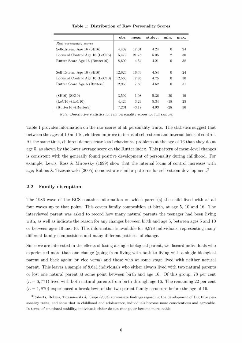
Table 1: Distribution of Raw Personality Scores
obs. mean st.dev. min. max.
Raw personality scores
Self-Esteem Age 16 (SE16) 4,439 17.81 4.24 0 24
Locus of Control Age 16 (LoC16) 5,479 21.78 5.05 2 30
Rutter Score Age 16 (Rutter16) 8,609 4.54 4.21 0 38
Self-Esteem Age 10 (SE10) 12,624 16.39 4.54 0 24
Locus of Control Age 10 (LoC10) 12,560 17.85 4.75 0 30
Rutter Score Age 5 (Rutter5) 12,965 7.83 4.62 0 31
(SE16)-(SE10) 3,592 1.08 5.36 -20 19
(LoC16)-(LoC10) 4,424 3.29 5.34 -18 25
(Rutter16)-(Rutter5) 7,231 -3.17 4.93 -28 36
Note: Descriptive statistics for raw personality scores for full sample.
Table 1 provides information on the raw scores of all personality traits. The statistics suggest that
between the ages of 10 and 16, children improve in terms of self-esteem and internal locus of control.
At the same time, children demonstrate less behavioural problems at the age of 16 than they do at
age 5, as shown by the lower average score on the Rutter index. This pattern of mean-level changes
is consistent with the generally found positive development of personality during childhood. For
example, Lewis, Ross & Mirowsky (1999) show that the internal locus of control increases with
age; Robins & Trzesniewski (2005) demonstrate similar patterns for self-esteem development.2
2.2 Family disruption
The 1986 wave of the BCS contains information on which parent(s) the child lived with at all
four waves up to that point. This covers family composition at birth, at age 5, 10 and 16. The
interviewed parent was asked to record how many natural parents the teenager had been living
with, as well as indicate the reason for any changes between birth and age 5, between ages 5 and 10
or between ages 10 and 16. This information is available for 8,978 individuals, representing many
different family compositions and many different patterns of change.
Since we are interested in the effects of losing a single biological parent, we discard individuals who
experienced more than one change (going from living with both to living with a single biological
parent and back again; or vice versa) and those who at some stage lived with neither natural
parent. This leaves a sample of 8,641 individuals who either always lived with two natural parents
or lost one natural parent at some point between birth and age 16. Of this group, 78 per cent
(n = 6, 771) lived with both natural parents from birth through age 16. The remaining 22 per cent
(n = 1, 870) experienced a breakdown of the two parent family structure before the age of 16.
2Roberts, Robins, Trzesniewski & Caspi (2003) summarize findings regarding the development of Big Five per-
sonality traits, and show that in childhood and adolescence, individuals become more conscientious and agreeable.
In terms of emotional stability, individuals either do not change, or become more stable.
6
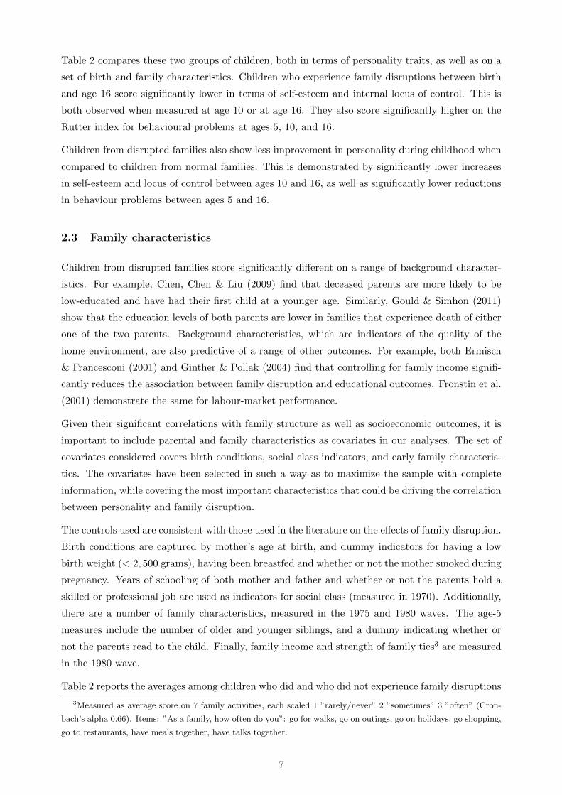
Table 2 compares these two groups of children, both in terms of personality traits, as well as on a
set of birth and family characteristics. Children who experience family disruptions between birth
and age 16 score significantly lower in terms of self-esteem and internal locus of control. This is
both observed when measured at age 10 or at age 16. They also score significantly higher on the
Rutter index for behavioural problems at ages 5, 10, and 16.
Children from disrupted families also show less improvement in personality during childhood when
compared to children from normal families. This is demonstrated by significantly lower increases
in self-esteem and locus of control between ages 10 and 16, as well as significantly lower reductions
in behaviour problems between ages 5 and 16.
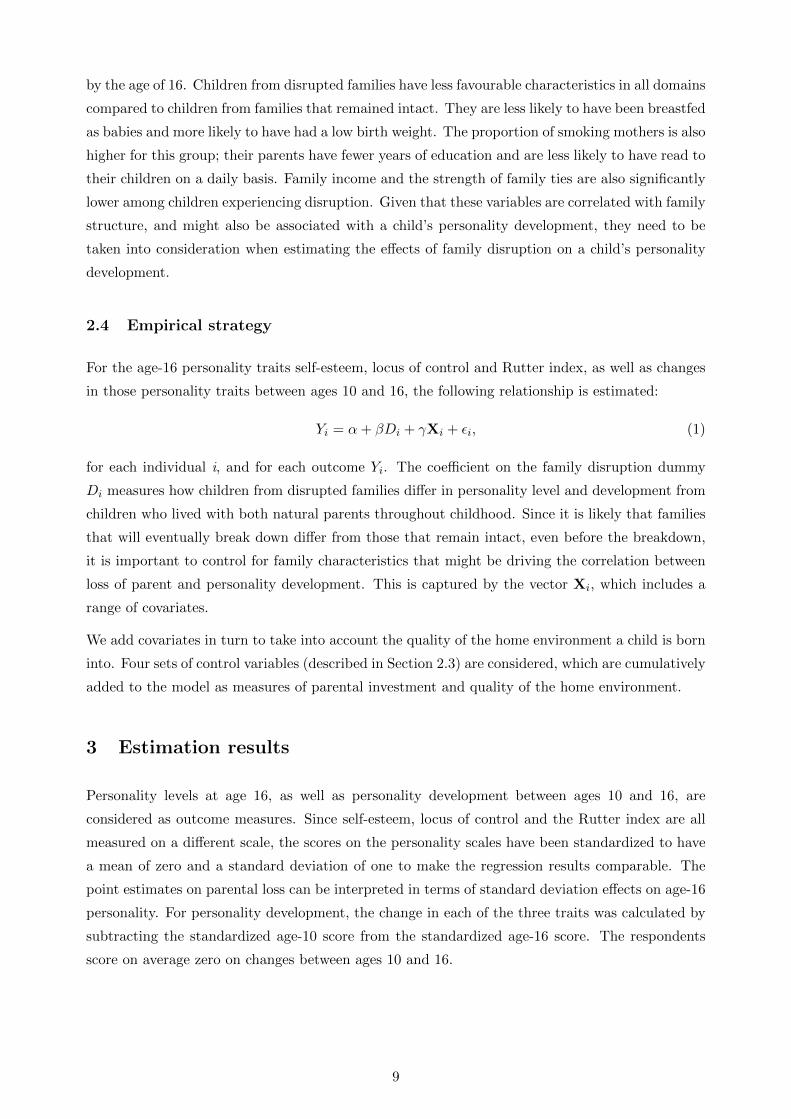
2.3 Family characteristics
Children from disrupted families score significantly different on a range of background character-
istics. For example, Chen, Chen & Liu (2009) find that deceased parents are more likely to be
low-educated and have had their first child at a younger age. Similarly, Gould & Simhon (2011)
show that the education levels of both parents are lower in families that experience death of either
one of the two parents. Background characteristics, which are indicators of the quality of the
home environment, are also predictive of a range of other outcomes. For example, both Ermisch
& Francesconi (2001) and Ginther & Pollak (2004) find that controlling for family income signifi-
cantly reduces the association between family disruption and educational outcomes. Fronstin et al.
(2001) demonstrate the same for labour-market performance.
Given their significant correlations with family structure as well as socioeconomic outcomes, it is
important to include parental and family characteristics as covariates in our analyses. The set of
covariates considered covers birth conditions, social class indicators, and early family characteris-
tics. The covariates have been selected in such a way as to maximize the sample with complete
information, while covering the most important characteristics that could be driving the correlation
between personality and family disruption.
The controls used are consistent with those used in the literature on the effects of family disruption.
Birth conditions are captured by mother’s age at birth, and dummy indicators for having a low
birth weight (< 2, 500 grams), having been breastfed and whether or not the mother smoked during
pregnancy. Years of schooling of both mother and father and whether or not the parents hold a
skilled or professional job are used as indicators for social class (measured in 1970). Additionally,
there are a number of family characteristics, measured in the 1975 and 1980 waves. The age-5
measures include the number of older and younger siblings, and a dummy indicating whether or
not the parents read to the child. Finally, family income and strength of family ties3 are measured
in the 1980 wave.
Table 2 reports the averages among children who did and who did not experience family disruptions
3Measured as average score on 7 family activities, each scaled 1 ”rarely/never” 2 ”sometimes” 3 ”often” (Cron-
bach’s alpha 0.66). Items: ”As a family, how often do you”: go for walks, go on outings, go on holidays, go shopping,
go to restaurants, have meals together, have talks together.
7

Table 2: Descriptives by Experience of Family Disruption
Experienced Family Disruption?
No Yes
mean sd obs. mean sd obs.
Raw personality scores
Self-Esteem Age 16 (SE16) 17.92 (4.12) 2,596 17.35−− (4.64) 596
Locus of Control Age 16 (LoC16) 22.15 (4.92) 3,365 20.87−− (5.38) 737
Rutter Score Age 16 (Rutter16) 4.24 (3.97) 6,091 5.35++ (4.66) 1,603
Self-Esteem Age 10 (SE10) 16.65 (4.52) 5,633 16.02−− (4.50) 1,489
Locus of Control Age 10 (LoC10) 18.24 (4.76) 5,603 17.42−− (4.61) 1,477
Rutter Score Age 10 (Rutter10) 425.45 (206.61) 6,055 466.31++ (225.90) 1,585
Rutter Score Age 5 (Rutter5) 7.59 (4.43) 5,827 8.38++ (4.81) 1,473
(SE16)-(SE10) 0.98 (5.36) 2,186 1.25 (5.44) 485
(LoC16)-(LoC10) 3.48 (5.26) 2,811 2.66−− (5.41) 588
(Rutter16)-(Rutter5) -3.29 (4.72) 5,274 −2.93++ (5.32) 1,276
Family Disruption 0.00 6,771 1.00 1,870
type of disruption (if disruption occurred after birth):
Death 6,771 0.18 (0.38) 1,421
Divorce 6,771 0.64 (0.48) 1,421
Separation 6,771 0.18 (0.39) 1,421
age at disruption:
At birth 6,771 0.10 (0.30) 1,870
Between 0 and 5 6,771 0.29 (0.45) 1,870
Between 5 and 10 6,771 0.27 (0.44) 1,870
Between 10 and 16 6,771 0.35 (0.48) 1,870
Birth conditions
Male 0.49 (0.50) 6,771 0.49 (0.50) 1,870
Mother’s age at birth 26.32 (5.21) 6,310 24.85−− (5.62) 1,726
Low birth weight (< 2, 500 grams) 0.06 (0.24) 6,340 0.07+ (0.26) 1,732
Breastfed dummy 0.39 (0.49) 5,864 0.36−− (0.48) 1,480
Mother smoked during pregnancy 0.37 (0.48) 6,321 0.49++ (0.50) 1,719
Social class (measured at birth)
Years of schooling mother 9.74 (1.78) 6,306 9.60−− (1.61) 1,724
Years of schooling father 10.02 (2.37) 6,196 9.73−− (1.99) 1,606
Parents skilled/professional 0.8 (0.40) 6,338 0.72−− (0.45) 1,731
Family characteristics (measured at age 5)
# of older siblings 0.99 (1.07) 5,879 1.05+ (1.22) 1,491
# of younger siblings 0.53 (0.64) 5,879 0.52 (0.65) 1,491
Read to every day 0.43 (0.49) 5,645 0.35−− (0.48) 1,426
Family characteristics (measured at age 10)
Gross weekly family income 3.16 (1.16) 5,657 2.51−− (1.31) 1,525
Strength of family ties 2.5 (0.30) 6,152 2.42−− (0.33) 1,619
Note: Descriptive statistics for main raw personality scores for full sample. Pluses and minuses indicate that
the average of respondents who experienced family disruption differs from the average of respondents who
lived with both natural parents throughout childhood. ++ (+) indicates that the average of the sample with
complete information is significantly larger at the 5% (10%) level, while −− (−) indicate that that average is
significantly smaller at the 5% (10%) level.
8
by the age of 16. Children from disrupted families have less favourable characteristics in all domains
compared to children from families that remained intact. They are less likely to have been breastfed
as babies and more likely to have had a low birth weight. The proportion of smoking mothers is also
higher for this group; their parents have fewer years of education and are less likely to have read to
their children on a daily basis. Family income and the strength of family ties are also significantly
lower among children experiencing disruption. Given that these variables are correlated with family
structure, and might also be associated with a child’s personality development, they need to be
taken into consideration when estimating the effects of family disruption on a child’s personality
development.
2.4 Empirical strategy
For the age-16 personality traits self-esteem, locus of control and Rutter index, as well as changes
in those personality traits between ages 10 and 16, the following relationship is estimated:
Yi = α+ βDi + γXi + εi, (1)
for each individual i, and for each outcome Yi. The coefficient on the family disruption dummy
Di measures how children from disrupted families differ in personality level and development from
children who lived with both natural parents throughout childhood. Since it is likely that families
that will eventually break down differ from those that remain intact, even before the breakdown,
it is important to control for family characteristics that might be driving the correlation between
loss of parent and personality development. This is captured by the vector Xi, which includes a
range of covariates.
We add covariates in turn to take into account the quality of the home environment a child is born
into. Four sets of control variables (described in Section 2.3) are considered, which are cumulatively
added to the model as measures of parental investment and quality of the home environment.
3 Estimation results
Personality levels at age 16, as well as personality development between ages 10 and 16, are
considered as outcome measures. Since self-esteem, locus of control and the Rutter index are all
measured on a different scale, the scores on the personality scales have been standardized to have
a mean of zero and a standard deviation of one to make the regression results comparable. The
point estimates on parental loss can be interpreted in terms of standard deviation effects on age-16
personality. For personality development, the change in each of the three traits was calculated by
subtracting the standardized age-10 score from the standardized age-16 score. The respondents
score on average zero on changes between ages 10 and 16.
9
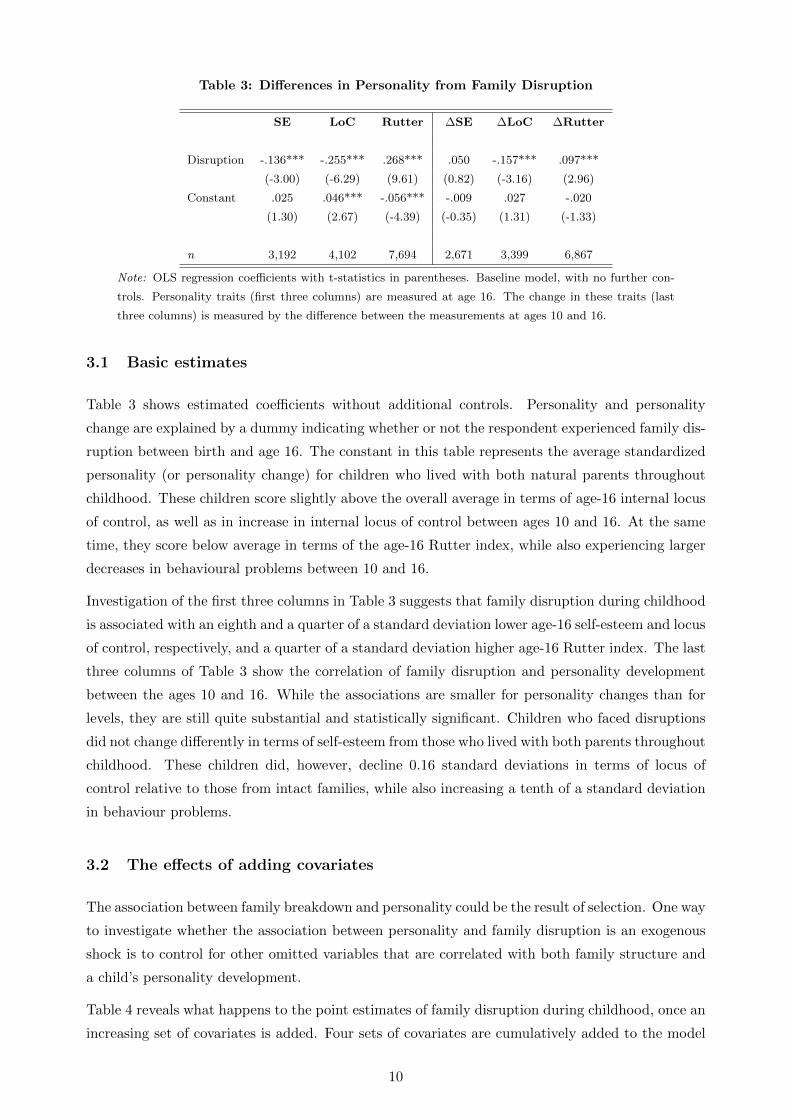
Table 3: Differences in Personality from Family Disruption
SE LoC Rutter ∆SE ∆LoC ∆Rutter
Disruption -.136*** -.255*** .268*** .050 -.157*** .097***
(-3.00) (-6.29) (9.61) (0.82) (-3.16) (2.96)
Constant .025 .046*** -.056*** -.009 .027 -.020
(1.30) (2.67) (-4.39) (-0.35) (1.31) (-1.33)
n 3,192 4,102 7,694 2,671 3,399 6,867
Note: OLS regression coefficients with t-statistics in parentheses. Baseline model, with no further con-
trols. Personality traits (first three columns) are measured at age 16. The change in these traits (last
three columns) is measured by the difference between the measurements at ages 10 and 16.
3.1 Basic estimates
Table 3 shows estimated coefficients without additional controls. Personality and personality
change are explained by a dummy indicating whether or not the respondent experienced family dis-
ruption between birth and age 16. The constant in this table represents the average standardized
personality (or personality change) for children who lived with both natural parents throughout
childhood. These children score slightly above the overall average in terms of age-16 internal locus
of control, as well as in increase in internal locus of control between ages 10 and 16. At the same
time, they score below average in terms of the age-16 Rutter index, while also experiencing larger
decreases in behavioural problems between 10 and 16.
Investigation of the first three columns in Table 3 suggests that family disruption during childhood
is associated with an eighth and a quarter of a standard deviation lower age-16 self-esteem and locus
of control, respectively, and a quarter of a standard deviation higher age-16 Rutter index. The last
three columns of Table 3 show the correlation of family disruption and personality development
between the ages 10 and 16. While the associations are smaller for personality changes than for
levels, they are still quite substantial and statistically significant. Children who faced disruptions
did not change differently in terms of self-esteem from those who lived with both parents throughout
childhood. These children did, however, decline 0.16 standard deviations in terms of locus of
control relative to those from intact families, while also increasing a tenth of a standard deviation
in behaviour problems.
3.2 The effects of adding covariates
The association between family breakdown and personality could be the result of selection. One way
to investigate whether the association between personality and family disruption is an exogenous
shock is to control for other omitted variables that are correlated with both family structure and
a child’s personality development.
Table 4 reveals what happens to the point estimates of family disruption during childhood, once an
increasing set of covariates is added. Four sets of covariates are cumulatively added to the model
10

as measures of parental investment and quality of the home environment. Including covariates
correlated with marital instability reduces the point estimates of the effects of family disruption on
age-16 personality. With the most elaborate set of control variables the effect of family disruption
on age-16 self-esteem is no longer statistically significantly different from zero. This suggests
that the correlation between family disruption and self-esteem is the result of omitted variables.
However, for locus of control and the Rutter index, the estimates remain significant and sizeable at
-.16 and .17 standard deviations, respectively. These effect sizes are comparable to the mean effect
sizes found in the review paper by Amato (2001). In an update of the meta-analysis of Amato &
Keith (1991), he finds that children experiencing divorce score about a fifth of a standard deviation
lower in terms of measured conduct and psychological adjustment and 0.15 standard deviations
lower in terms of social relations.
The covariates that seem to be predictive of personality traits across the board are parental educa-
tion, parental care (proxied by reading to the five-year-old child on a daily basis) and the strength
of family ties at age 10. Additionally, the number of siblings, and especially the number of younger
siblings, has a detrimental effect on personality traits. Finally, there is also an important role for
family income, which was also observed by Ginther & Pollak (2004), who found that controlling
for family income the effect of living in a single-parent family was often no longer significant.
The sets of covariates are added to mitigate the omitted variable bias in the point estimates for
family disruption and cover various aspects of the home environment before the age of 10. To
the extent that the effects of family characteristics prior to age 10 are already reflected in age-10
personality, the association between parental loss and personality change between ages 10 and 16
will be unaffected by the addition of the sets of controls. This is both reflected in the coefficients
on the controls, which are largely insignificant, as well as on the dummy for family disruption
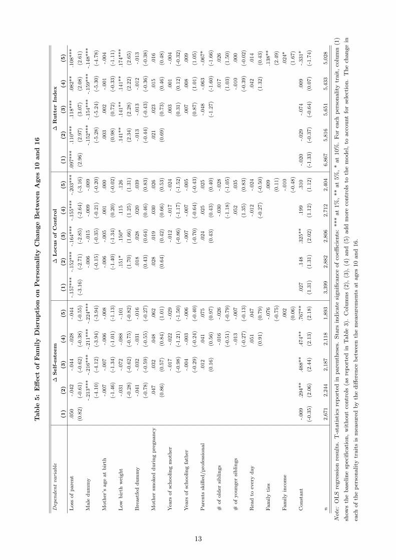
when we investigate changes in personality between age 10 and 16. Table 5 shows the estimated
coefficients.
With regard to changes in self-esteem, locus of control, and the Rutter index, the expanding set
of controls does not significantly change the point estimates of family disruption. Regarding self-
esteem, the effect was not significantly different from zero to begin with in Table 4. Combined
with the insignificant effect on age-16 self-esteem, the correlation between family disruption and
self-esteem seems to be a reflection of omitted variables. However, the point estimates for changes
in locus of control and the Rutter index remain sizeable and significant. This could be interpreted
as evidence of a causal relationship between family disruption and locus of control and behaviour
problems, but may still also be driven by other factors.
Selection plays a role in explaining the observed correlation between family disruption and per-
sonality development. The reduction of the point estimates suggests that family disruption is not
fully exogenous. However, the estimated coefficients remain sizeable and significant, which provides
support for the argument that the negative effects associated with family disruption are not merely
reflecting a priori differences between families. To limit the effect of selection, the specification
with the most elaborate set of covariates will be used for the remaining analyses on heterogeneity.
The endogeneity of family disruption is investigated in more detail in Section 5.
11

Tab
le4:
Eff
ect
of
Fam
ily
Dis
rup
tion
on
Pers
on
ali
tyL
evel
at
Age
16
Depen
den
tva
riable
Self-esteem
(at
age
16)
LocusofControl
(at
age
16)
RutterIn
dex
(at
age
16)
(1)
(2)
(3)
(4)
(5)
(1)
(2)
(3)
(4)
(5)
(1)
(2)
(3)
(4)
(5)
Loss
of
pare
nt
-.136***
-.173***
-.164***
-.146***
-.039
-.255***
-.226***
-.220***
-.196***
-.161***
.268***
.244***
.226***
.208***
.170***
(-3.0
0)
(-3.3
2)
(-3.0
9)
(-2.6
7)
(-0.6
5)
(-6.2
9)
(-4.9
3)
(-4.7
6)
(-4.1
6)
(-3.0
9)
(9.6
1)
(7.7
2)
(6.9
7)
(6.2
6)
(4.6
2)
Male
du
mm
y.0
06
.000
.009
.025
.059*
.047
.055
.057
-.008
-.012
-.013
-.021
(0.1
5)
(0.0
1)
(0.2
4)
(0.5
7)
(1.7
1)
(1.3
9)
(1.5
8)
(1.5
5)
(-0.3
3)
(-0.4
7)
(-0.5
1)
(-0.7
4)
Moth
er’s
age
at
bir
th.0
05
.005
.004
.003
.009***
.006*
.011***
.012***
-.011***
-.011***
-.008***
-.010***
(1.3
9)
(1.1
7)
(0.8
8)
(0.6
2)
(2.7
3)
(1.9
0)
(2.8
9)
(2.7
5)
(-4.6
0)
(-4.3
4)
(-2.7
4)
(-3.0
7)
Low
bir
thw
eight
-.201**
-.196**
-.232***
-.189**
-.064
-.080
-.113
-.081
.164***
.164***
.203***
.214***
(-2.3
8)
(-2.2
8)
(-2.6
6)
(-2.0
4)
(-0.8
8)
(-1.1
0)
(-1.5
4)
(-1.0
2)
(3.1
6)
(3.1
4)
(3.7
7)
(3.7
0)
Bre
ast
fed
du
mm
y.0
59
.016
.011
.015
.173***
.094***
.080**
.077**
-.045*
-.011
-.010
-.014
(1.4
8)
(0.3
8)
(0.2
6)
(0.3
3)
(4.9
9)
(2.6
6)
(2.2
2)
(1.9
9)
(-1.7
6)
(-0.4
3)
(-0.3
6)
(-0.4
8)
Moth
ersm
oked
du
rin
gp
regn
an
cy-.
069*
-.056
-.038
-.006
-.142***
-.097***
-.068*
-.084**
.150***
.131***
.115***
.089***
(-1.6
5)
(-1.3
2)
(-0.8
7)
(-0.1
3)
(-3.9
6)
(-2.7
0)
(-1.8
4)
(-2.1
2)
(5.8
0)
(4.9
6)
(4.2
6)
(3.0
6)
Yea
rsof
sch
oolin
gm
oth
er.0
10
.002
-.014
.058***
.049***
.038***
-.022**
-.018*
-.018*
(0.7
3)
(0.1
8)
(-1.0
0)
(5.0
3)
(4.1
9)
(3.0
3)
(-2.3
8)
(-1.9
0)
(-1.7
9)
Yea
rsof
sch
oolin
gfa
ther
.028***
.027***
.015
.036***
.034***
.025***
-.018***
-.017**
-.015*
(2.8
5)
(2.7
2)
(1.3
9)
(4.2
3)
(3.9
5)
(2.6
2)
(-2.6
4)
(-2.4
5)
(-1.9
4)
Pare
nts
skille
d/p
rofe
ssio
nal
.080
.082
.072
.185***
.152***
.122**
-.125***
-.104***
-.094***
(1.5
0)
(1.5
0)
(1.2
2)
(4.0
6)
(3.2
6)
(2.4
3)
(-3.8
7)
(-3.1
2)
(-2.6
2)
#of
old
ersi
bli
ngs
-.049**
-.039
-.105***
-.096***
.010
.003
(-2.0
7)
(-1.5
2)
(-5.1
6)
(-4.3
7)
(0.7
0)
(0.2
2)
#of
you
nger
sib
lin
gs
-.062*
-.015
-.086***
-.080**
.091***
.066***
(-1.6
8)
(-0.3
7)
(-2.7
3)
(-2.3
5)
(4.0
6)
(2.7
0)
Rea
dto
ever
yd
ay
.117***
.079*
.125***
.106***
-.072***
-.033
(2.7
9)
(1.7
4)
(3.5
1)
(2.7
5)
(-2.6
6)
(-1.1
2)
Fam
ily
ties
.219***
.025
-.259***
(2.8
4)
(0.3
8)
(-5.3
1)
Fam
ily
inco
me
.089***
.084***
-.019
(4.5
6)
(4.9
1)
(-1.4
3)
Con
stant
.025
-.101
-.515***
-.413**
-1.0
65***
.046***
-.241***
-1.2
40***
-1.1
71***
-1.3
69***
-.056***
.190***
.676***
.523***
1.2
92***
(1.3
0)
(-0.9
3)
(-3.4
6)
(-2.5
0)
(-4.0
1)
(2.6
7)
(-2.5
9)
(-9.5
5)
(-8.1
7)
(-6.0
8)
(-4.3
9)
(2.8
3)
(6.7
7)
(4.7
9)
(7.6
6)
n3,1
92
2,6
25
2,5
54
2,4
73
2,1
50
4,1
02
3,4
08
3,3
14
3,2
06
2,7
68
7,6
94
6,3
56
6,1
71
5,9
29
5,0
88
Note:
OL
Sre
gre
ssio
nre
sult
s.T
-sta
tist
ics
rep
ort
edin
pare
nth
eses
.Sta
rsin
dic
ate
signifi
cance
of
coeffi
cien
ts:
***
at
1%
,**
at
5%
,*
at
10%
.F
or
each
per
sonality
trait
,co
lum
n(1
)
show
sth
ebase
line
spec
ifica
tion,
wit
hout
contr
ols
(as
rep
ort
edin
Table
3).
Colu
mns
(2),
(3),
(4)
and
(5)
add
more
contr
ols
toth
em
odel
,to
acc
ount
for
sele
ctio
n.
12
Tab
le5:
Eff
ect
of
Fam
ily
Dis
rup
tion
on
Pers
on
ali
tyC
han
ge
Betw
een
Ages
10
an
d16
Depen
den
tva
riable
∆Self-esteem
∆LocusofControl
∆RutterIn
dex
(1)
(2)
(3)
(4)
(5)
(1)
(2)
(3)
(4)
(5)
(1)
(2)
(3)
(4)
(5)
Loss
of
pare
nt
.050
-.042
-.044
-.028
-.044
-.157***
-.152***
-.164***
-.155***
-.203***
.097***
.110***
.118***
.082**
.108***
(0.8
2)
(-0.6
1)
(-0.6
2)
(-0.3
8)
(-0.5
5)
(-3.1
6)
(-2.7
1)
(-2.8
5)
(-2.6
4)
(-3.1
6)
(2.9
6)
(2.9
7)
(3.0
7)
(2.0
8)
(2.6
1)
Male
du
mm
y-.
213***
-.216***
-.211***
-.224***
-.006
-.015
-.009
-.009
-.152***
-.154***
-.159***
-.148***
(-4.1
0)
(-4.1
2)
(-3.9
4)
(-3.9
4)
(-0.1
5)
(-0.3
5)
(-0.2
1)
(-0.2
0)
(-5.2
8)
(-5.2
4)
(-5.3
0)
(-4.7
8)
Moth
er’s
age
at
bir
th-.
007
-.007
-.006
-.008
-.006
-.005
.001
.000
.003
.002
-.001
-.004
(-1.4
6)
(-1.3
4)
(-1.0
1)
(-1.1
3)
(-1.4
0)
(-1.3
4)
(0.2
0)
(-0.0
2)
(0.9
8)
(0.7
2)
(-0.3
3)
(-1.1
1)
Low
bir
thw
eight
-.031
-.072
-.088
-.101
.151*
.150*
.115
.126
.141**
.141**
.141**
.174***
(-0.2
8)
(-0.6
2)
(-0.7
5)
(-0.8
2)
(1.7
0)
(1.6
6)
(1.2
5)
(1.3
1)
(2.3
4)
(2.2
8)
(2.2
2)
(2.6
5)
Bre
ast
fed
du
mm
y-.
041
-.032
-.031
-.016
.018
.028
.020
.039
-.013
-.013
-.012
-.013
(-0.7
8)
(-0.5
9)
(-0.5
5)
(-0.2
7)
(0.4
3)
(0.6
4)
(0.4
6)
(0.8
3)
(-0.4
4)
(-0.4
3)
(-0.3
6)
(-0.3
8)
Moth
ersm
oked
du
rin
gp
regn
an
cy.0
47
.032
.048
.062
.028
.019
.030
.026
.021
.023
.015
.016
(0.8
6)
(0.5
7)
(0.8
4)
(1.0
1)
(0.6
4)
(0.4
2)
(0.6
6)
(0.5
3)
(0.6
9)
(0.7
3)
(0.4
6)
(0.4
8)
Yea
rsof
sch
oolin
gm
oth
er-.
017
-.022
-.029
-.012
-.017
-.024
.003
.001
-.004
(-0.9
8)
(-1.2
1)
(-1.5
0)
(-0.8
6)
(-1.1
7)
(-1.5
2)
(0.3
1)
(0.1
2)
(-0.3
2)
Yea
rsof
sch
oolin
gfa
ther
-.004
-.003
-.006
-.007
-.007
-.005
.007
.008
.009
(-0.2
9)
(-0.2
4)
(-0.4
0)
(-0.7
0)
(-0.6
4)
(-0.4
3)
(0.8
7)
(1.0
1)
(1.0
5)
Pare
nts
skille
d/p
rofe
ssio
nal
.012
.041
.075
.024
.025
.025
-.048
-.063
-.067*
(0.1
6)
(0.5
6)
(0.9
7)
(0.4
3)
(0.4
3)
(0.4
0)
(-1.2
7)
(-1.6
0)
(-1.6
6)
#of
old
ersi
blin
gs
-.016
-.026
-.030
-.028
.017
.026
(-0.5
1)
(-0.7
9)
(-1.1
8)
(-1.0
5)
(1.0
3)
(1.5
0)
#of
you
nger
sib
lin
gs
-.013
-.007
.052
.035
-.010
.000
(-0.2
7)
(-0.1
3)
(1.3
5)
(0.8
3)
(-0.3
9)
(-0.0
2)
Rea
dto
ever
yd
ay
.051
.047
-.012
-.024
.042
.014
(0.9
1)
(0.7
9)
(-0.2
7)
(-0.5
0)
(1.3
2)
(0.4
3)
Fam
ily
ties
-.076
.009
.138**
(-0.7
5)
(0.1
1)
(2.4
9)
Fam
ily
inco
me
.002
-.010
.024*
(0.0
6)
(-0.4
8)
(1.6
7)
Con
stant
-.009
.294**
.488**
.474**
.767**
.027
.148
.325**
.199
.310
-.020
-.029
-.074
.009
-.331*
(-0.3
5)
(2.0
6)
(2.4
4)
(2.1
3)
(2.1
8)
(1.3
1)
(1.3
1)
(2.0
2)
(1.1
2)
(1.1
2)
(-1.3
3)
(-0.3
7)
(-0.6
4)
(0.0
7)
(-1.7
4)
n2,6
71
2,2
44
2,1
87
2,1
18
1,8
93
3,3
99
2,8
82
2,8
06
2,7
12
2,4
04
6,8
67
5,8
16
5,6
51
5,4
33
5,0
28
Note:
OL
Sre
gre
ssio
nre
sult
s.T
-sta
tist
ics
rep
ort
edin
pare
nth
eses
.Sta
rsin
dic
ate
signifi
cance
of
coeffi
cien
ts:
***
at
1%
,**
at
5%
,*
at
10%
.F
or
each
per
sonality
trait
,co
lum
n(1
)
show
sth
ebase
line
spec
ifica
tion,
wit
hout
contr
ols
(as
rep
ort
edin
Table
3).
Colu
mns
(2),
(3),
(4)
and
(5)
add
more
contr
ols
toth
em
odel
,to
acc
ount
for
sele
ctio
n.
The
change
in
each
of
the
per
sonality
trait
sis
mea
sure
dby
the
diff
eren
ceb
etw
een
the
mea
sure
men
tsat
ages
10
and
16.
13
4 Heterogeneity
In this section we investigate the effects of heterogeneity in the type disruption, the age at which
the child is confronted with disruption and possible differences between boys and girls.
4.1 Type of disruption
For children experiencing family disruption after birth, the reason for family disruption is also
known in most cases. It is the result of a separation of parents, divorce of parents or the death
of one of two natural parents. Divorce was the reason for family disruption in two-thirds of these
cases. The remaining third of cases are equally divided between a separation of parents and death
of one of the parents.
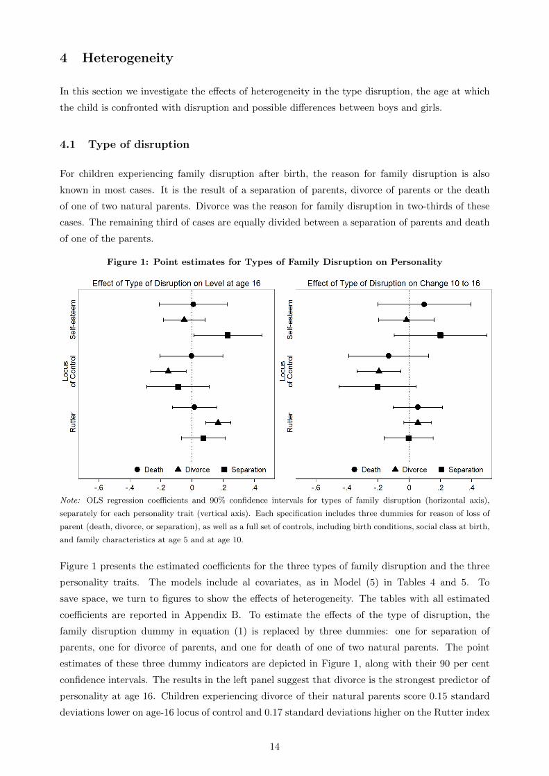
Figure 1: Point estimates for Types of Family Disruption on Personality
Note: OLS regression coefficients and 90% confidence intervals for types of family disruption (horizontal axis),
separately for each personality trait (vertical axis). Each specification includes three dummies for reason of loss of
parent (death, divorce, or separation), as well as a full set of controls, including birth conditions, social class at birth,
and family characteristics at age 5 and at age 10.
Figure 1 presents the estimated coefficients for the three types of family disruption and the three
personality traits. The models include al covariates, as in Model (5) in Tables 4 and 5. To
save space, we turn to figures to show the effects of heterogeneity. The tables with all estimated
coefficients are reported in Appendix B. To estimate the effects of the type of disruption, the
family disruption dummy in equation (1) is replaced by three dummies: one for separation of
parents, one for divorce of parents, and one for death of one of two natural parents. The point
estimates of these three dummy indicators are depicted in Figure 1, along with their 90 per cent
confidence intervals. The results in the left panel suggest that divorce is the strongest predictor of
personality at age 16. Children experiencing divorce of their natural parents score 0.15 standard
deviations lower on age-16 locus of control and 0.17 standard deviations higher on the Rutter index
14
for behavioural problems, compared to children from homes that remained intact. The effects of
experiencing death of a parent or separation of parents are both economically and statistically
insignificant. These findings are consistent with those from Corak (2001), whose difference-in-
difference estimates reveal that the associations between family disruption and income and own
marital stability are greater in the case of divorce than in case of death of a parent. Regarding
education, Francesconi et al. (2010) also find that it is divorce, and not parental loss through death,
that leads to lower schooling attainment.
In terms of personality changes (right panel in Figure 1), the effects of the different reasons for
family disruption are mostly insignificant. The figure presents the estimated coefficients including
the full set of covariates. The only significant result is that children experiencing divorce of their
parents, decline 0.2 standard deviations in terms of internal locus of control, compared to children
from normal families. The point estimates of experiencing death of a parent or separation of parents
are generally comparable in magnitude, yet not significantly different from zero. The lack of effects
in terms of personality change could be due to the fact that the effects of family disruption have
already manifested themselves by the age of 10. It could also be the case that crucial variables are
missing from the analysis, such as unobserved pre-existing health conditions of the parents, family
stress or marital instability, which may have affected childhood personality prior to the actual
change (e.g. Chen et al., 2009). Both arguments point to selection being the driving force behind
the observed correlation between parental loss and personality development.
4.2 Age
The BCS also provides information on the timing of family disruption. To estimate the effects of
age of the child at the time of disruption, the family disruption dummy in equation (1) is replaced
by four age dummies, representing four groups: children born into a single-parent family (10 per
cent), and children facing family disruption between birth and age 5 (28 per cent), between 5 and
10 (28 per cent) or between 10 and 16 (33 per cent). Figure 2 presents the estimated coefficients for
the four age groups separately for both personality traits at age 16 and the change in personality
between age 10 and 16.
The pattern of effects for the different ages at which family disruption occurs differs between the
three personality measures. For age-16 self-esteem, being born into a single-parent home, as well
as losing one of two natural parents from the household between ages 10 and 16 is associated with
statistically significantly lower age-16 self-esteem, while a loss occurring between birth and age 5,
or between ages 5 and 10, does not lead to significantly different self-esteem scores, in comparison
to children from normal families. For locus of control, however, experiencing disruption between
age 5 and 10 seems to be detrimental, in addition to being born into a one-natural parent home.
A change between 5 and 10 is again insignificant when it comes to predicting age-16 Rutter scores.
The relatively volatile patterns across personality measures documented in Figure 2 suggest that it
is important to measure the timing of family disruption. Generally, the effects of family disruption
seem to be less severe if the child was older at the time of the change. More specifically, disruption at
15
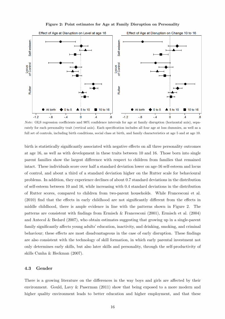
Figure 2: Point estimates for Age at Family Disruption on Personality
Note: OLS regression coefficients and 90% confidence intervals for age at family disruption (horizontal axis), sepa-
rately for each personality trait (vertical axis). Each specification includes all four age at loss dummies, as well as a
full set of controls, including birth conditions, social class at birth, and family characteristics at age 5 and at age 10.
birth is statistically significantly associated with negative effects on all three personality outcomes
at age 16, as well as with development in these traits between 10 and 16. Those born into single
parent families show the largest difference with respect to children from families that remained
intact. These individuals score over half a standard deviation lower on age-16 self-esteem and locus
of control, and about a third of a standard deviation higher on the Rutter scale for behavioural
problems. In addition, they experience declines of about 0.7 standard deviations in the distribution
of self-esteem between 10 and 16, while increasing with 0.4 standard deviations in the distribution
of Rutter scores, compared to children from two-parent households. While Francesconi et al.
(2010) find that the effects in early childhood are not significantly different from the effects in
middle childhood, there is ample evidence in line with the patterns shown in Figure 2. The
patterns are consistent with findings from Ermisch & Francesconi (2001), Ermisch et al. (2004)
and Antecol & Bedard (2007), who obtain estimates suggesting that growing up in a single-parent
family significantly affects young adults’ education, inactivity, and drinking, smoking, and criminal
behaviour; these effects are most disadvantageous in the case of early disruption. These findings
are also consistent with the technology of skill formation, in which early parental investment not
only determines early skills, but also later skills and personality, through the self-productivity of
skills Cunha & Heckman (2007).
4.3 Gender
There is a growing literature on the differences in the way boys and girls are affected by their
environment. Gould, Lavy & Paserman (2011) show that being exposed to a more modern and
higher quality environment leads to better education and higher employment, and that these
16
effects are stronger for girls. Estimating the effect of parental education and occupation on child
education, McIntosh & Munk (2007) and Gould & Simhon (2011) obtain estimates suggesting that
boys and girls respond differently to their environments. When it comes to childhood intervention
programs, there are some mixed results. The Abecedarian program boosted IQ, but primarily for
girls (Cunha et al., 2006). Results at age 27 from participants in the Perry Preschool Program
are also generally more favourable for girls, yet this pattern reverses when outcomes at age 40
are considered. This section contributes to this discussion by looking at gender differences in the
effects of parental loss.
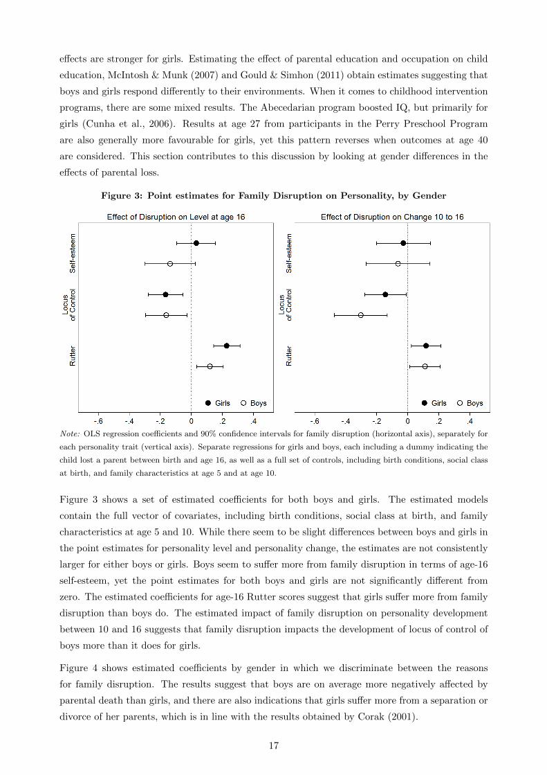
Figure 3: Point estimates for Family Disruption on Personality, by Gender
Note: OLS regression coefficients and 90% confidence intervals for family disruption (horizontal axis), separately for
each personality trait (vertical axis). Separate regressions for girls and boys, each including a dummy indicating the
child lost a parent between birth and age 16, as well as a full set of controls, including birth conditions, social class
at birth, and family characteristics at age 5 and at age 10.
Figure 3 shows a set of estimated coefficients for both boys and girls. The estimated models
contain the full vector of covariates, including birth conditions, social class at birth, and family
characteristics at age 5 and 10. While there seem to be slight differences between boys and girls in
the point estimates for personality level and personality change, the estimates are not consistently
larger for either boys or girls. Boys seem to suffer more from family disruption in terms of age-16
self-esteem, yet the point estimates for both boys and girls are not significantly different from
zero. The estimated coefficients for age-16 Rutter scores suggest that girls suffer more from family
disruption than boys do. The estimated impact of family disruption on personality development
between 10 and 16 suggests that family disruption impacts the development of locus of control of
boys more than it does for girls.
Figure 4 shows estimated coefficients by gender in which we discriminate between the reasons
for family disruption. The results suggest that boys are on average more negatively affected by
parental death than girls, and there are also indications that girls suffer more from a separation or
divorce of her parents, which is in line with the results obtained by Corak (2001).
17
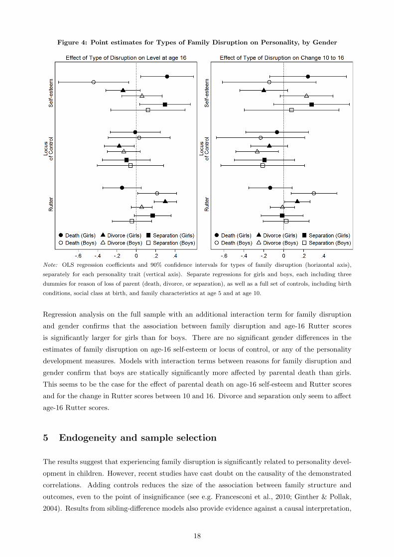
Figure 4: Point estimates for Types of Family Disruption on Personality, by Gender
Note: OLS regression coefficients and 90% confidence intervals for types of family disruption (horizontal axis),
separately for each personality trait (vertical axis). Separate regressions for girls and boys, each including three
dummies for reason of loss of parent (death, divorce, or separation), as well as a full set of controls, including birth
conditions, social class at birth, and family characteristics at age 5 and at age 10.
Regression analysis on the full sample with an additional interaction term for family disruption
and gender confirms that the association between family disruption and age-16 Rutter scores
is significantly larger for girls than for boys. There are no significant gender differences in the
estimates of family disruption on age-16 self-esteem or locus of control, or any of the personality
development measures. Models with interaction terms between reasons for family disruption and
gender confirm that boys are statically significantly more affected by parental death than girls.
This seems to be the case for the effect of parental death on age-16 self-esteem and Rutter scores
and for the change in Rutter scores between 10 and 16. Divorce and separation only seem to affect
age-16 Rutter scores.
5 Endogeneity and sample selection
The results suggest that experiencing family disruption is significantly related to personality devel-
opment in children. However, recent studies have cast doubt on the causality of the demonstrated
correlations. Adding controls reduces the size of the association between family structure and
outcomes, even to the point of insignificance (see e.g. Francesconi et al., 2010; Ginther & Pollak,
2004). Results from sibling-difference models also provide evidence against a causal interpretation,
18
finding that the correlations between family structure and child outcomes are not significant (see
e.g. Bjorklund et al., 2007; Bjorklund & Sundstrom, 2006). While the results demonstrated in
Table 4 show a reduction of the effect size when additional controls are added to the model, a
significant relationship between family disruption and personality development remains. If family
disruption is simply capturing the effect of omitted variables, or if the effect is driven by selection
in the regression sample, there is no support for a causal interpretation of the uncovered correla-
tions. This section first investigates the endogeneity of family structure with the use of placebo
regressions. Second, the role of sample selection is discussed.
5.1 Placebo effects
If family disruption can be identified as an exogenous shock, any association between family dis-
ruption and personality traits arrives after the change in family structure. Under the assumption
of a causal relationship between family disruption and personality outcomes and change, family
disruption after age 10 should not be significantly related to personality measured at age 10.
Our strategy is to estimate models including those children who lived with both natural parents
until at least the age of 10. This yields estimates of the effect of family disruption on personality
traits and development between the age of 10 and 16. Now, a statistically significant effect of family
disruption between 10 and 16 on personality at age 10 would indicate that family disruption is
likely to be endogenous.
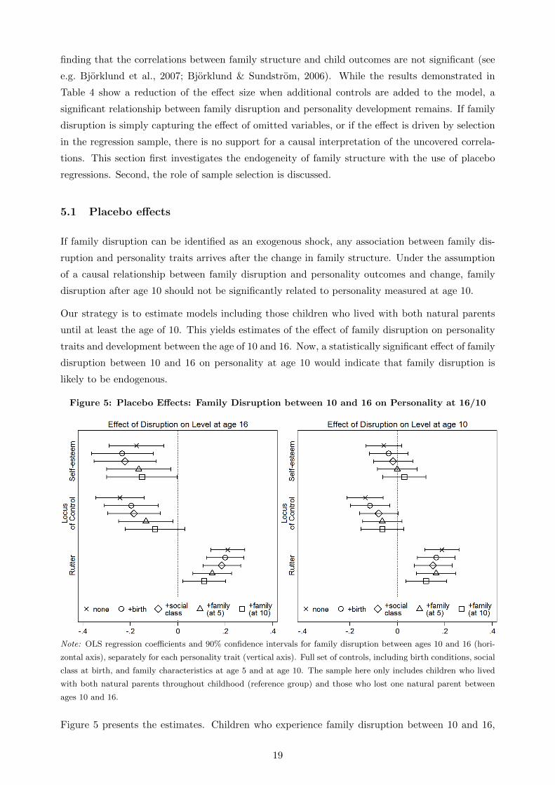
Figure 5: Placebo Effects: Family Disruption between 10 and 16 on Personality at 16/10
Note: OLS regression coefficients and 90% confidence intervals for family disruption between ages 10 and 16 (hori-
zontal axis), separately for each personality trait (vertical axis). Full set of controls, including birth conditions, social
class at birth, and family characteristics at age 5 and at age 10. The sample here only includes children who lived
with both natural parents throughout childhood (reference group) and those who lost one natural parent between
ages 10 and 16.
Figure 5 presents the estimates. Children who experience family disruption between 10 and 16,
19
score statistically significantly lower in terms of self-esteem and locus of control and significantly
higher on the Rutter scale for behaviour problems, when measured at age 16 (left panel). Expanding
the set of covariates reduces the correlation between family disruption and age-16 personality,
which mitigates the omitted variable bias. For locus of control, the effect is no longer statistically
significant.
To test whether family disruption is endogenous, personality traits at age 10 are regressed on
family disruption after age 10. The right panel in Figure 5 suggests that these correlations are
much smaller than those with age-16 personality. Inclusion of the full vector of covariates yields
a zero point estimate for self-esteem. The estimated coefficient for age-10 locus of control is half
of what it is for age-16 locus of control, and not statistically significantly different from zero.
These results support the assumption that family disruption is exogenous and that the estimated
coefficients for self-esteem and locus of control could be interpreted as causal. For Rutter scores,
this relationship does not seem to hold. The point estimates are equal in magnitude, whether
Rutter scores are measured at age 10 or 16, which suggests that family disruption is endogenous
in the sense that behavioural problems do not become worse due to family disruption.
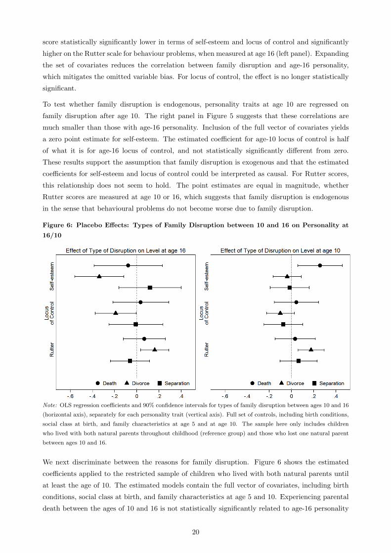
Figure 6: Placebo Effects: Types of Family Disruption between 10 and 16 on Personality at
16/10
Note: OLS regression coefficients and 90% confidence intervals for types of family disruption between ages 10 and 16
(horizontal axis), separately for each personality trait (vertical axis). Full set of controls, including birth conditions,
social class at birth, and family characteristics at age 5 and at age 10. The sample here only includes children
who lived with both natural parents throughout childhood (reference group) and those who lost one natural parent
between ages 10 and 16.
We next discriminate between the reasons for family disruption. Figure 6 shows the estimated
coefficients applied to the restricted sample of children who lived with both natural parents until
at least the age of 10. The estimated models contain the full vector of covariates, including birth
conditions, social class at birth, and family characteristics at age 5 and 10. Experiencing parental
death between the ages of 10 and 16 is not statistically significantly related to age-16 personality
20
(left panel). The association with age-10 personality (right panel) is also mostly insignificant, and
even turns positive in case of self-esteem and locus of control. These results support the notion that
death of a parent is an exogenous event. Divorce and separation, however, seem to be endogenous.
For divorce, the point estimates on age-16 personality traits average at .23 standard deviations.
For Rutter scores, the associations with age-10 and age-16 scores are similar in magnitude and
significance (at .17 standard deviations), while the point estimates for age-10 self-esteem and locus
of control reduce significantly and are no longer significantly different from zero. These results
suggest that especially divorce is an endogenous event.
5.2 Sample selection
The analyses in this paper have been based on a sample from the BCS. To the extent that this
selection is not random, the estimates could be biased. Table 6 provides averages for all variables
for the total sample and averages for the samples that remain after several rounds of selection. At
the same time, each column shows whether the average within the selected sample is significantly
different from the average of individuals with incomplete information in that selection round. This
gives an idea of the extent of selection and possibly also the direction of bias due to non-response
or attrition.
The first round of selection involves selecting respondents with valid information on family disrup-
tion, as obtained from the 1986 parental questionnaire (Disruption). Second, controlling for birth
conditions, social class, and family characteristics at age 5 and 10 reduces the sample available for
analyses even further (Controls). Finally, information is needed on age-16 personality traits (P16),
and for the analyses on personality development, also on age-10 personality traits (P10).
Information on family structure during childhood is required. This information is only available
for 46 per cent of the total sample (8,641 out of 18,724). Within this sample (Loss), the share of
children experiencing family disruption is 22 per cent. Benson (2010) points out that it is often
cited that one in four children in the UK live with one natural parent at any one time. A less well
known statistic is the proportion of children who will live with one natural parent before age 16.
Benson (2010) uses data from cohorts born in the 1980s to demonstrate that among these cohorts,
this statistic is as high as 40 per cent, and estimates that by 2009, one half of all children will
experience family disruption by the age of 16. Andersson (2002) provides a similar statistic for
15 other European countries and the United States. The average among those countries is 27 per
cent.
Compared to these statistics, the share of 22 per cent obtained from parental reports from the
1986 wave of the British Cohort Study is low. The cohorts reported on by Benson (2010) are
younger than the BCS70 cohort, and the United Kingdom was not among the countries reported
on by Andersson (2002), which makes a direct comparison impossible. A statistic that can be
more easily verified is the percentage of births outside marriage. Historical statistics for England
and Wales show that this percentage was 8.3 per cent for 1970 (Office for National Statistics,
2010). This share in the BCS is comparable at 7.4 per cent, when using information reported
21
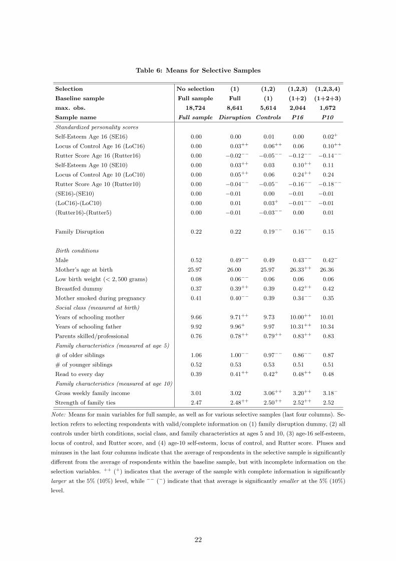
Table 6: Means for Selective Samples
Selection No selection (1) (1,2) (1,2,3) (1,2,3,4)
Baseline sample Full sample Full (1) (1+2) (1+2+3)
max. obs. 18,724 8,641 5,614 2,044 1,672
Sample name Full sample Disruption Controls P16 P10
Standardized personality scores
Self-Esteem Age 16 (SE16) 0.00 0.00 0.01 0.00 0.02+
Locus of Control Age 16 (LoC16) 0.00 0.03++ 0.06++ 0.06 0.10++
Rutter Score Age 16 (Rutter16) 0.00 −0.02−− −0.05−− −0.12−− −0.14−−
Self-Esteem Age 10 (SE10) 0.00 0.03++ 0.03 0.10++ 0.11
Locus of Control Age 10 (LoC10) 0.00 0.05++ 0.06 0.24++ 0.24
Rutter Score Age 10 (Rutter10) 0.00 −0.04−− −0.05− −0.16−− −0.18−−
(SE16)-(SE10) 0.00 −0.01 0.00 −0.01 −0.01
(LoC16)-(LoC10) 0.00 0.01 0.03+ −0.01−− −0.01
(Rutter16)-(Rutter5) 0.00 −0.01 −0.03−− 0.00 0.01
Family Disruption 0.22 0.22 0.19−− 0.16−− 0.15
Birth conditions
Male 0.52 0.49−− 0.49 0.43−− 0.42−
Mother’s age at birth 25.97 26.00 25.97 26.33++ 26.36
Low birth weight (< 2, 500 grams) 0.08 0.06−− 0.06 0.06 0.06
Breastfed dummy 0.37 0.39++ 0.39 0.42++ 0.42
Mother smoked during pregnancy 0.41 0.40−− 0.39 0.34−− 0.35
Social class (measured at birth)
Years of schooling mother 9.66 9.71++ 9.73 10.00++ 10.01
Years of schooling father 9.92 9.96+ 9.97 10.31++ 10.34
Parents skilled/professional 0.76 0.78++ 0.79++ 0.83++ 0.83
Family characteristics (measured at age 5)
# of older siblings 1.06 1.00−− 0.97−− 0.86−− 0.87
# of younger siblings 0.52 0.53 0.53 0.51 0.51
Read to every day 0.39 0.41++ 0.42+ 0.48++ 0.48
Family characteristics (measured at age 10)
Gross weekly family income 3.01 3.02 3.06++ 3.20++ 3.18−
Strength of family ties 2.47 2.48++ 2.50++ 2.52++ 2.52
Note: Means for main variables for full sample, as well as for various selective samples (last four columns). Se-
lection refers to selecting respondents with valid/complete information on (1) family disruption dummy, (2) all
controls under birth conditions, social class, and family characteristics at ages 5 and 10, (3) age-16 self-esteem,
locus of control, and Rutter score, and (4) age-10 self-esteem, locus of control, and Rutter score. Pluses and
minuses in the last four columns indicate that the average of respondents in the selective sample is significantly
different from the average of respondents within the baseline sample, but with incomplete information on the
selection variables. ++ (+) indicates that the average of the sample with complete information is significantly
larger at the 5% (10%) level, while −− (−) indicate that that average is significantly smaller at the 5% (10%)
level.
22
by all mothers present in the 1970 wave. Among respondents with valid information from the
1986 wave on family structure, this share is only 4.4 per cent, indicating that unmarried mothers
are underrepresented in the regression samples. This is consistent with the lower observed share
of children experiencing family disruption (22 per cent). That selection on family disruption is
non-random, is also confirmed by the second column in Table 6.
The under-sampling of instable families becomes more important after the second round of selec-
tion. Of the respondents with data on family disruption, only 65 per cent have complete data on
the full set of controls (5,614 out of 8,641). Only 19 per cent of these respondents experience family
disruption before age 16; compared to 27 per cent for the 35 per cent of respondents with incom-
plete information on covariates. Further restricting the sample to those with valid information on
self-esteem, locus of control, and Rutter scores, reduces the share of children experiencing family
disruption to 16 per cent when age-16 personality information is required (sample P16), and to 15
per cent when, additionally, information on age-10 personality is required (sample P10).
Attrition and sample selection are not only related to the share of respondents experiencing family
disruption, but also to personality traits, as well as birth conditions and early childhood family
characteristics. Respondents still in the sample after selection on family disruption information
(sample Loss) rank significantly higher in the distribution of self-esteem and locus of control,
and lower in the distribution of Rutter scores. The differences with the full sample are further
exacerbated once selection on the set of control variables is applied (sample Controls). The same
pattern is observed for childhood characteristics, with the average home environment becoming
more favourable after each selection round. While this does not hold for all control variables,
average parental education and social class, and parental care increase with each selection round.
Given that sample selection is non-random, the effects of family disruption estimated in this study
could be biased. The share of children in the regression sample experiencing the event of interest
is likely to be lower than that same share in the total UK population. If the children within
the sample do not differ systematically on unobservables that codetermine personality, the point
estimates obtained from the regression sample have been estimated with less precision, but are not
necessarily biased. There are, however, indications that those leaving the sample are more likely to
be from the families at risk. If the effects of family disruption are more likely to be present at the
bottom of the family quality distribution, our estimates provide a lower bound for the true effect
of family disruption. Given that most of the selection in the sample lies with the crucial variable
on family disruption, it is impossible to correct for selection on this variable.
The addition of an increasing set of covariates to the model has revealed a pattern of reductions
in the estimated effect sizes of family disruption, providing support to the argument that the
correlation between family disruption and personality is caused by selection, rather than causation.
However, adding more controls also reduces the sample available for analysis, and the observed
pattern might simply be the result of selecting ”better” families, for which the effect might be
smaller to begin with (even without controls). This can be tested by re-estimating the model for
the five sets of covariates for the restricted sample of respondents with valid information on the
most complete vector of covariates (i.e., the sample Controls in Table 6). Figure 7 reports these
23

results and reveals the same pattern as shown in Section 3 (Tables 4 and 5). Overall, the reduction
in effect size resulting from additional covariates does not seem to be the result of differences in
the composition of the samples.
Figure 7: Point estimates of Family Disruption on Personality, Restricted Sample
Note: OLS regression coefficients and 90% confidence intervals for family disruption (horizontal axis), separately for
each personality trait (vertical axis), and for different sets of controls. Only respondents with complete information
on the full set of controls – including birth conditions, social class at birth, and family characteristics at age 5 and
at age 10 – were considered in the analyses.
6 Conclusion, interpretation and future research
This research contributes to the discussion on the development of personality traits during child-
hood. First, using a variety of personality traits, measured at ages 10 and 16, the descriptive
statistics indicate that children go through a significant positive development as they age. Self-
esteem and internal locus of control rise, while behavioural problems decline between ages 10 and
16. Second, the regression analyses suggest that this positive development is negatively affected
by a shock to the family environment. Finally, the correlations between family disruption and
personality development are to some extent endogenous.
Family disruption is defined as having experienced a switch from living with both natural parents
to living with only one natural parent before the age of 16. In terms of self-esteem, internal locus of
control and behavioural problems, children experiencing family disruption score significantly worse
and show less favourable development than children who lived in an intact family throughout
childhood. These associations hide more detailed patterns. The effects of family disruption on
personality development are generally stronger when the reason is divorce, compared to the case
of death of one of the parents. In line with results from Corak (2001), conditioning on gender,
the pattern arises that boys suffer more from the death of a parent than girls do, while there are
also indications that divorce of parents affects girls more than boys. The age at which the change
24

occurs also matters, with the effects of losing a parent generally being less severe when the child
is older at the time of family breakdown.
Other dimensions that may influence the estimated effect of family disruption have not been
discussed. In this study, families are split into two groups: those with two natural parents and
those with only one natural parent. There are a number of different possible family compositions
among families with only one natural parent. A child may live with its natural mother or its natural
father, either with or without a step-father or step-mother or other parental figures. If an additional
parent figure has a positive effect on child development, through for example additional parental
investments, the correlations reported here are underestimates of the impact of family disruption.
However, the role of an extra (non-natural) parent figure need not necessarily be positive. Beller
& Chung (1992) find mixed effects of the presence of a stepfather for various educational outcome
measures, and these effects also depend on the gender of the child. Gennetian (2005) finds that
relying on traditional classifications of family structure may lead to biased effect sizes. While the
sample sizes in the BCS are too small to estimate the effects of these specific family compositions,
Ginther & Pollak (2004) find that the crucial distinction is between children who grow up in
traditional nuclear families (i.e., living with both natural parents) and children who grow up in
other family structures (i.e., single parent families or blended families).
Since family structure is endogenous, simple correlations of family disruption with personality de-
velopment do not represent the causal effect of a change in the family structure. With the addition
of family characteristics that are correlated with both family structure and children’s outcomes,
the point estimates of experiencing family breakdown are significantly reduced. Given that much of
the associations remain significant after controlling for a range of family characteristics, one might
argue in favour of a causal interpretation of the remaining correlations. However, placebo analyses
reveal that the problem of endogeneity is not fully addressed with our set of control variables.
Apparently, part of the association between personality and parental loss already manifests itself
before the change in family structure actually occurred. This suggests that there are other factors
that correlate with family dissolution as well as with childhood personality development. Given
that the negative association between family dissolution and both personality level and personality
change is partially the result of selection, future research is needed to uncover the reasons behind
the fact that children from intact families experience a more positive development and why children
from homes that eventually break down face a fall in the personality distribution. Some of the
factors controlled for in this paper help contribute to this discussion, such as the mediating role of
parental education and parental social class as well as number of siblings, and parental care.
These findings are in line with results found by Gould & Simhon (2011), who argue in favour of a
causal role of parental education in shaping children’s schooling, which is dependent on the time
spent with each parent. Corak (2001) shows that family income accounts for part of the association
between family disruption and personality development. Cobb-Clark & Ribar (2012) show that
financial stress and unsatisfactory relationships with parents are related to youths’ transitions from
home and school. McCulloch & Joshi (2002) demonstrate that low income has detrimental effects
on the cognitive development of children, and that these effects may be mitigated by positive
25
parental behaviours. This study adds to the literature casting doubt on a causal interpretation
of the correlation between family breakdown and child outcomes. Nevertheless, this study also
shows that personality traits are in development in childhood and that the direction and strength
of development depends on factors exogenous to the child. While personality improves with age,
parental investment plays a mediating or stimulating role.
References
Almlund, M., Duckworth, A. L., Heckman, J. J., & Kautz, T. D. (2011). Personality psychology
and economics. IZA Discussion Paper No. 5500.
Amato, P. & Keith, B. (1991). Parental divorce and the well-being of children: A meta-analysis.
Psychological Bulletin, 110 (1), 26–46.
Amato, P. R. (2001). Children of divorce in the 1990s: An update of the Amato and Keith (1991)
meta-analysis. Journal of Family Psychology, 15 (3), 355 – 370.
Andersson, G. (2002). Children’s experience of family disruption and family formation: Evidence
from 16 FFS countries. Demographic Research, 7, 343 – 364.
Antecol, H. & Bedard, K. (2007). Does single parenthood increase the probability of teenage
promiscuity, substance use, and crime?. Journal of Population Economics, 20 (1), 55 – 71.
Beller, A. H. & Chung, S. S. (1992). Family structure and educational attainment of children:
Effects of remarriage. Journal of Population Economics, 5 (1), 39 – 59.
Benson, H. (2010). Family breakdown in the UK: It’s not about divorce. Report, Bristol Community
Family Trust.
Bjorklund, A., Ginther, D. K., & Sundstrom, M. (2007). Family structure and child outcomes in
the USA and Sweden. Journal of Population Economics, 20 (1), 183 – 201.
Bjorklund, A. & Sundstrom, M. (2006). Parental separation and children’s educational attainment:
A siblings analysis on Swedish register data. Economica, 73 (292), 605 – 624.
Borghans, L., Duckworth, A. L., Heckman, J. J., & Ter Weel, B. (2008). The economics and
psychology of personality traits. Journal of Human Resources, 43 (4), 972 – 1059.
Chen, S. H., Chen, Y.-C., & Liu, J.-T. (2009). The impact of unexpected maternal death on
education: First evidence from three national administrative data links. American Economic
Review, 99 (2), 149 – 153.
Cobb-Clark, D. A. & Ribar, D. C. (2012). Financial stress, family relationships, and australian
youths’ transitions from home and school. Review of Economics of the Household, 10 (4), 469 –
490.
Cobb-Clark, D. A. & Schurer, S. (2012). The stability of big-five personality traits. Economics
Letters, 115 (1), 11 – 15.
Cobb-Clark, D. A. & Tan, M. (2011). Noncognitive skills, occupational attainment, and relative
wages. Labour Economics, 18 (1), 1 – 13.
Conti, G., Heckman, J. J., & Urzua, S. (2010). Early endowments, education, and health. Working
Papers 2011-001, Human Capital and Economic Opportunity Working Group.
26
Corak, M. (2001). Death and divorce: The long-term consequences of parental loss on adolescents.
Journal of Labor Economics, 19 (3), 682 – 715.
Cunha, F. & Heckman, J. J. (2007). The technology of skill formation. American Economic Review,
97 (2), 31 – 47.
Cunha, F., Heckman, J. J., Lochner, L., & Masterov, D. V. (2006). Interpreting the evidence on
life cycle skill formation. In E. Hanushek & F. Welch (Eds.), Handbook of the Economics of
Education (pp. 697–812).
Currie, J. & Stabile, M. (2006). Child mental health and human capital accumulation: The case
of ADHD. Journal Of Health Economics, 25 (6), 1094 – 1118.
Ermisch, J., Francesconi, M., & Pevalin, D. J. (2004). Parental partnership and joblessness in
childhood and their influence on young people’s outcomes. Journal of the Royal Statistical
Society: Series A (Statistics in Society), 167 (1), 69 – 101.
Ermisch, J. F. & Francesconi, M. (2001). Family structure and children’s achievements. Journal
of Population Economics, 14 (2), 249.
Feinstein, L. (2000). The relative economic importance of academic, psychological and behavioural
attributes developed on childhood. Discussion paper 443, Centre for Economic Performance,
London School of Economics and Political Science, London, UK.
Flouri, E. & Buchanan, A. (2004). Early father’s and mother’s involvement and child’s later
educational outcomes. British Journal of Educational Psychology, 74, 141 – 153.
Francesconi, M., Jenkins, S. P., & Siedler, T. (2010). Childhood family structure and schooling
outcomes: Evidence for Germany. Journal of Population Economics, 23 (3), 1073 – 1103.
Fronstin, P., Greenberg, D. H., & Robins, P. K. (2001). Parental disruption and the labour market
performance of children when they reach adulthood. Journal of Population Economics, 14 (1),
137.
Gammage, P. (1975). Socialisation, schooling and locus of control. PhD thesis, Bristol University.
Gennetian, L. (2005). One or two parents? half or step siblings? the effect of family structure on
young children’s achievement. Journal of Population Economics, 18 (3), 415 – 436.
Ginther, D. K. & Pollak, R. A. (2004). Family structure and children’s educational outcomes:
blended families, stylized facts, and descriptive regressions. Demography, 41 (4), 671 – 696.
Gould, E. D., Lavy, V., & Paserman, M. D. (2011). Sixty years after the magic carpet ride: The
long-run effect of the early childhood environment on social and economic outcomes. Review of
Economic Studies, 78 (3), 938 – 973.
Gould, E. D. & Simhon, A. (2011). Does quality time produce quality children? Evidence on
the intergenerational transmission of human capital using parental deaths. CEPR Discussion
Papers: 8258.
Knudsen, E. I., Heckman, J. J., Cameron, J. L., & Shonkoff, J. P. (2006). Economic, neurobio-
logical, and behavioral perspectives on building America’s future workforce. Procedings of the
National Academy of Sciences of the United States of America, 103 (27), 10155 – 10162.
Lewis, S., Ross, C., & Mirowsky, J. (1999). Establishing a sense of personal control in the transition
to adulthood. Social Forces, 77, 1573 – 1599.
McCulloch, A. & Joshi, H. E. (2002). Child development and family resources: Evidence from the
27
second generation of the 1958 British Birth Cohort. Journal of Population Economics, 15 (2),
283 – 304.
McIntosh, J. & Munk, M. D. (2007). Scholastic ability vs family background in educational success:
evidence from Danish sample survey data. Journal of Population Economics, 20 (1), 101 – 120.
Murasko, J. E. (2007). A lifecourse study on education and health: The relationship between
childhood psychosocial resources and outcomes in adolescence and young adulthood. Social
Science Research, 36, 1348 – 1370.
Office for National Statistics (2010). Table 1. summary of key birth statistics, 1938-2010. In Birth
summary tables, England and Wales, 2010.
Roberts, B., Robins, R., Trzesniewski, K., & Caspi, A. (2003). Personality Trait Development in
Adulthood, chapter 26, (pp. 579–596). New York: Kluwer Academic/Plenum Publishers.
Roberts, B. W. & DelVecchio, W. F. (2000). The rank-order consistency of personality traits
from childhood to old age: A quantitative review of longitudinal studies. Psychological Bulletin,
126 (1), 3 – 25.
Roberts, B. W., Walton, K. E., & Viechtbauer, W. (2006). Patterns of mean-level change in
personality traits across the life course: A meta-analysis of longitudinal studies. Psychological
Bulletin, 132 (1), 1 – 25.
Robins, R. & Trzesniewski, K. (2005). Self-esteem development across the lifespan. Current
Directions in Psychological Science, 14, 158 – 162.
Rutter, M., Tizard, J., & Whitmore, K. (1970). Education, health and behaviour. London: Long-
man.
Specht, J., Schmukle, S. C., & Egloff, B. (2011). Stability and change of personality across the life
course: The impact of age and major life events on mean-level and rank-order stability of the
Big Five. Journal of Personality & Social Psychology, 101 (4), 862 – 882.
Von Stumm, S., Gale, C. R., Batty, G. D., & Deary, I. J. (2009). Childhood intelligence, locus of
control and behaviour disturbance as determinants of intergenerational social mobility: British
Cohort Study 1970. Intelligence, 329 – 340.
28

A Rutter, Self-esteem, and Locus of control
Three measures are used to capture personality traits: self-esteem, internal locus of control, and
a Rutter index for behavioural problems. Self-esteem measures an individual’s sense of self-worth,
internal locus of control measures a child’s perceived achievement control, and the Rutter index
gives an indication of behavioural problems.
Self-esteem assesses respondents’ self-esteem with reference to teachers, peers and parents and
consists of 12 items, while locus of control measures children’s perceived achievement control with
a list of 15 items. Items are scaled 0 ”yes” 1 ”don’t know” 2 ”no”, except the first self-esteem item
”Parent like to hear about ideas” and the locus of control item ”Believe in planning ahead”, which
are reversely coded. Higher scores thus indicate higher self-esteem and higher internal locus of
control. Table A.1 shows the inter-item correlations or covariances for these sets of items, and the
Cronbach’s alpha statistic for the scale formed from them, both for ages 10 and 16. The self-esteem
and locus of control scores are constructed by summing the scores on the set of 12/15 items, and
then standardizing the resulting score to have mean zero and standard deviation one.
At ages 5, 10, and 16, the respondents’ parents, usually the mother, are asked to indicate to what
extent a certain description applies to the respondent. At ages 5 and 16, the items are scaled
0 ”does not apply” 1 ”applies somewhat” 2 ”certainly applies”. The age-10 items are scaled 1
through 100, where 1 indicates ”does not apply” and 100 indicates ”certainly applies”. Higher
scores indicate more severe behavioural problems. Table A.2 shows the inter-item correlations or
covariances for the 19 items, and the Cronbach’s alpha statistic for the scale formed from them.
The three Rutter scores, at ages 5, 10, and 16, are constructed by summing the scores on the 19
mother-rated items, and then standardizing the resulting score to have mean zero and standard
deviation one. The correlation coefficients between the resulting measures for self-esteem, locus of
control, and behavioural problems (Rutter) are reported in Table A.3.
For each set of of items, we apply multiple imputation through chained equations to impute missing
values, using the remaining items as predictors for the item of interest. By doing so, we increase
the number of observations with valid personality measures. For each item i within each set
of Rutter/self-esteem/locus of control items, we estimate the following model to predict missing
values:
Itemi = αi +∑j 6=i
βjItemj + εi
This process starts with the item with least amount of missing observations. Missing observations
are then imputed, and the process continues to the item with next fewest missing observations.
For the age-10 Rutter score we apply the above model using linear regression, since the items are
scaled from 1 through 100. Imputed values below 1 are set to 1, and those above 100 are set to
100. For the age-5 and age-16 Rutter scores, and the age-10 and age-16 self-esteem and locus of
control scores, we use multinomial logit regression to impute missing values.
29
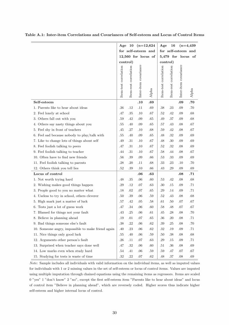
Table A.1: Inter-item Correlations and Covariances of Self-esteem and Locus of Control Items
Age 10 (n=12,624
for self-esteem and
12,560 for locus of
control)
Age 16 (n=4,439
for self-esteem and
5,479 for locus of
control)
Item
-tes
tco
rrel
ati
on
Item
-res
tco
rrel
ati
on
Inte
r-it
emco
vari
ance
Alp
ha
Item
-tes
tco
rrel
ati
on
Item
-res
tco
rrel
ati
on
Inte
r-it
emco
vari
ance
Alp
ha
Self-esteem .10 .69 .09 .70
1. Parents like to hear about ideas .26 .12 .11 .69 .38 .23 .09 .70
2. Feel lonely at school .47 .35 .10 .67 .52 .42 .09 .68
3. Others fall out with you .59 .42 .09 .65 .49 .37 .09 .68
4. Others say nasty things about you .55 .40 .09 .65 .57 .43 .08 .67
5. Feel shy in front of teachers .45 .27 .10 .68 .59 .42 .08 .67
6. Feel sad because nobody to play/talk with .55 .40 .09 .65 .48 .32 .09 .69
7. Like to change lots of things about self .49 .31 .10 .67 .48 .30 .09 .69
8. Feel foolish talking to peers .47 .31 .10 .67 .52 .32 .08 .69
9. Feel foolish talking to teacher .44 .31 .10 .67 .58 .44 .08 .67
10. Often have to find new friends .56 .39 .09 .66 .53 .33 .09 .69
11. Feel foolish talking to parents .28 .20 .11 .68 .33 .23 .10 .70
12. Others think you tell lies .52 .39 .10 .66 .43 .29 .09 .69
Locus of control .06 .63 .08 .71
1. Not worth trying hard .48 .35 .06 .60 .53 .42 .08 .68
2. Wishing makes good things happen .29 .12 .07 .63 .30 .15 .09 .71
3. People good to you no matter what .18 .02 .07 .65 .29 .14 .09 .71
4. Useless to try in school, others cleverer .50 .39 .06 .59 .52 .43 .08 .68
5. High mark just a matter of luck .57 .42 .05 .58 .61 .50 .07 .67
6. Tests just a lot of guess work .47 .34 .06 .60 .58 .48 .07 .67
7. Blamed for things not your fault .43 .25 .06 .61 .45 .28 .08 .70
8. Believe in planning ahead .19 .01 .07 .65 .36 .20 .08 .71
9. Bad things someone else’s fault .38 .22 .06 .62 .39 .25 .08 .70
10. Someone angry, impossible to make friend again .40 .23 .06 .62 .32 .19 .09 .71
11. Nice things only good luck .55 .40 .06 .59 .50 .38 .08 .68
12. Arguments other person’s fault .26 .11 .07 .63 .29 .15 .09 .71
13. Surprised when teacher says done well .47 .32 .06 .60 .51 .36 .08 .69
14. Low marks even when study hard .54 .41 .06 .59 .59 .47 .07 .67
15. Studying for tests is waste of time .32 .22 .07 .62 .48 .37 .08 .69
Note: Sample includes all individuals with valid information on the individual items, as well as imputed values
for individuals with 1 or 2 missing values in the set of self-esteem or locus of control items. Values are imputed
using multiple imputation through chained equations using the remaining items as regressors. Items are scaled
0 ”yes” 1 ”don’t know” 2 ”no”, except the first self-esteem item ”Parents like to hear about ideas” and locus
of control item ”Believe in planning ahead”, which are reversely coded. Higher scores thus indicate higher
self-esteem and higher internal locus of control.
30
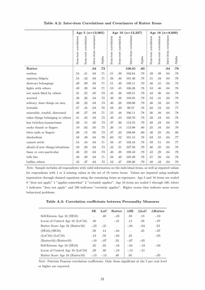
Table A.2: Inter-item Correlations and Covariances of Rutter Items
Age 5 (n=12,965) Age 10 (n=13,337) Age 16 (n=8,609)
Item
-tes
tco
rrel
ati
on
Item
-res
tco
rrel
ati
on
Inte
r-it
emco
vari
ance
Alp
ha
Item
-tes
tco
rrel
ati
on
Item
-res
tco
rrel
ati
on
Inte
r-it
emco
vari
ance
Alp
ha
Item
-tes
tco
rrel
ati
on
Item
-res
tco
rrel
ati
on
Inte
r-it
emco
vari
ance
Alp
ha
Rutter .04 .73 106.61 .80 .04 .79
restless .54 .41 .04 .71 .51 .39 102.64 .79 .49 .39 .04 .78
squirmy/fidgety .54 .42 .04 .71 .56 .46 101.40 .78 .51 .43 .04 .78
destroys belongings .49 .39 .04 .71 .51 .46 109.11 .79 .46 .41 .04 .78
fights with others .49 .39 .04 .71 .53 .45 106.26 .78 .53 .46 .04 .78
not much liked by others .31 .25 .05 .72 .45 .38 109.51 .79 .42 .36 .04 .78
worried .38 .26 .04 .72 .49 .38 103.85 .79 .52 .41 .04 .78
solitary, does things on own .36 .22 .04 .73 .40 .28 108.06 .79 .46 .33 .04 .79
irritable .57 .45 .04 .70 .59 .49 99.57 .78 .62 .52 .04 .77
miserable, tearful, distressed .46 .37 .04 .71 .55 .48 106.11 .78 .56 .49 .04 .78
takes things belonging to others .41 .32 .04 .72 .49 .43 109.76 .79 .50 .44 .04 .78
has twitches/mannerisms .20 .15 .05 .73 .37 .30 112.55 .79 .28 .23 .04 .79
sucks thumb or fingers .19 .02 .05 .75 .26 .14 113.98 .80 .25 .16 .04 .79
bites nails or fingers .30 .15 .05 .73 .37 .23 108.68 .80 .40 .25 .04 .80
disobedient .58 .49 .04 .70 .60 .52 101.15 .78 .63 .55 .04 .77
cannot settle .54 .44 .04 .71 .56 .47 102.44 .78 .59 .51 .04 .77
afraid of new things/situations .33 .20 .04 .73 .42 .31 107.56 .79 .46 .35 .04 .78
fussy or over-particular .36 .22 .04 .73 .40 .28 108.43 .79 .42 .29 .04 .79
tells lies .48 .39 .04 .71 .56 .49 105.29 .78 .57 .50 .04 .78
bullies others .45 .37 .04 .72 .52 .47 109.20 .79 .48 .42 .04 .78
Note: Sample includes all respondents with valid information on the individual items, as well as imputed values
for respondents with 1 or 2 missing values in the set of 19 rutter items. Values are imputed using multiple
imputation through chained equations using the remaining items as regressors. Age 5 and 16 items are scaled
0 ”does not apply” 1 ”applies somewhat” 2 ”certainly applies”. Age 10 items are scaled 1 through 100, where
1 indicates ”does not apply” and 100 indicates ”certainly applies”. Higher scores thus indicate more severe
behavioral problems.
Table A.3: Correlation coefficients between Personality Measures
SE LoC Rutter ∆SE ∆LoC ∆Rutter
Self-Esteem Age 16 (SE16) . .40 -.23 .58 .13 -.10
Locus of Control Age 16 (LoC16) .40 . -.21 .14 .59 -.07
Rutter Score Age 16 (Rutter16) -.23 -.21 . -.04 -.04 .53
(SE16)-(SE10) .58 .14 -.04 . .25 -.07
(LoC16)-(LoC10) .13 .59 -.04 .25 . -.05
(Rutter16)-(Rutter10) -.10 -.07 .53 -.07 -.05 .
Self-Esteem Age 10 (SE10) .25 .22 -.16 -.64 -.19 -.03
Locus of Control Age 10 (LoC10) .29 .40 -.18 -.13 -.51 .
Rutter Score Age 10 (Rutter10) -.13 -.13 .40 .05 . -.05
Note: Pairwise Pearson correlation coefficients. Only those significant at the 5 per cent level
or higher are reported.
31
B Supporting Tables
This section provides the full regression tables which were used to create the figures in this paper.
• Figure 1 (Types of Family Disruption): Tables B.1 and B.2
• Figure 2 (Age at Family Disruption): Tables B.3 and B.4
• Figure 3 (Family Disruption, by Gender): Tables B.5 and B.6
• Figure 4 (Types of Family Disruption, by Gender): Tables B.7 and B.8
• Figure 5 (Placebo Effects: Family Disruption): Tables B.9 and B.10
• Figure 6 (Placebo Effects: Types of Family Disruption): Tables B.11 and B.12
• Figure 7 (Family Disruption, Restricted Sample): Tables B.13 and B.14
32
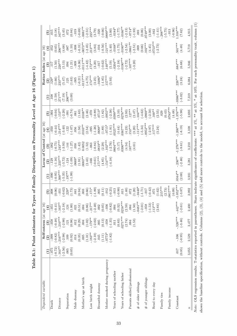
Tab
leB
.1:
Poin
test
imate
sfo
rT
yp
es
of
Fam
ily
Dis
rup
tion
on
Pers
on
ali
tyL
evel
at
Age
16
(Fig
ure
1)
Depen
den
tva
riable
Self-esteem
(at
age
16)
LocusofControl
(at
age
16)
RutterIn
dex
(at
age
16)
(1)
(2)
(3)
(4)
(5)
(1)
(2)
(3)
(4)
(5)
(1)
(2)
(3)
(4)
(5)
Dea
th-.
075
-.099
-.058
-.051
.008
-.090
-.129
-.082
-.050
-.004
.108
.129*
.117
.052
.015
(-0.7
2)
(-0.8
2)
(-0.4
8)
(-0.4
1)
(0.0
6)
(-0.9
5)
(-1.1
6)
(-0.7
5)
(-0.4
4)
(-0.0
4)
(1.5
9)
(1.6
6)
(1.5
0)
(0.6
5)
(0.1
8)
Div
orc
e-.
164**
-.216***
-.210***
-.163**
-.051
-.300***
-.233***
-.243***
-.214***
-.153**
.271***
.233***
.220***
.206***
.167***
(-2.5
6)
(-2.9
8)
(-2.9
0)
(-2.1
8)
(-0.6
2)
(-5.3
5)
(-3.7
2)
(-3.9
3)
(-3.4
0)
(-2.2
0)
(7.1
9)
(5.4
7)
(5.1
3)
(4.6
8)
(3.4
5)
Sep
ara
tion
.005
.109
.121
.124
.229*
-.197**
-.124
-.144
-.122
-.091
.206***
.125
.094
.087
.072
(0.0
5)
(0.9
2)
(0.9
8)
(1.0
0)
(1.7
3)
(-1.9
9)
(-1.0
9)
(-1.2
7)
(-1.0
7)
(-0.7
4)
(3.0
0)
(1.6
3)
(1.2
1)
(1.1
0)
(0.8
4)
Male
du
mm
y.0
14
.012
.021
.041
.0669*
.050
.056
.061
-.005
-.009
-.008
-.019
(0.3
5)
(0.2
9)
(0.5
1)
(0.9
4)
(1.9
1)
(1.4
2)
(1.5
8)
(1.6
3)
(-0.2
1)
(-0.3
6)
(-0.3
1)
(-0.6
9)
Moth
er’s
age
at
bir
th.0
05
.004
.004
.003
.0083**
0.0
052
.0103**
.0108**
-.0117***
-.0111***
-.0073**
-.0081**
(1.3
1)
(1.0
2)
(0.8
6)
(0.6
6)
(2.4
3)
(1.5
2)
(2.5
4)
(2.4
6)
(-4.7
5)
(-4.4
2)
(-2.4
5)
(-2.5
1)
Low
bir
thw
eight
-.183**
-.179**
-.217**
-.171*
-.046
-.063
-.095
-.070
.174***
.172***
.213***
.225***
(-2.1
0)
(-2.0
2)
(-2.4
0)
(-1.8
0)
(-0.6
1)
(-0.8
4)
(-1.2
6)
(-0.8
8)
(3.2
5)
(3.2
0)
(3.8
4)
(3.7
9)
Bre
ast
fed
du
mm
y.0
45
.005
.002
.005
.171***
.0819**
.0688*
.0713*
-.0486*
-.017
-.016
-.020
(1.1
1)
(0.1
3)
(0.0
5)
(0.1
1)
(4.8
5)
(2.2
9)
(1.8
9)
(1.8
2)
(-1.8
5)
(-0.6
2)
(-0.5
6)
(-0.6
6)
Moth
ersm
oked
du
rin
gp
regn
an
cy-.
0773*
-.058
-.036
-.012
-.154***
-.102***
-.0715*
-.0955**
.157***
.140***
.121***
.0889***
(-1.8
2)
(-1.3
5)
(-0.8
2)
(-0.2
5)
(-4.1
8)
(-2.7
6)
(-1.9
1)
(-2.3
8)
(5.9
3)
(5.1
9)
(4.4
0)
(3.0
0)
Yea
rsof
sch
oolin
gm
oth
er.0
11
.004
-.013
.0604***
.0525***
.0399***
-.0204**
-.0168*
-.0184*
(0.8
3)
(0.3
2)
(-0.9
0)
(5.1
7)
(4.4
4)
(3.1
0)
(-2.1
8)
(-1.7
5)
(-1.7
7)
Yea
rsof
sch
oolin
gfa
ther
.0271***
.0258***
.015
.0390***
.0367***
.0276***
-.0190***
-.0180**
-.0166**
(2.7
4)
(2.5
9)
(1.4
0)
(4.5
4)
(4.2
3)
(2.9
3)
(-2.7
2)
(-2.5
4)
(-2.1
3)
Pare
nts
skille
d/p
rofe
ssio
nal
.084
.084
.072
.187***
.153***
.127**
-.107***
-.0861**
-.0714*
(1.5
3)
(1.5
0)
(1.2
0)
(4.0
1)
(3.2
0)
(2.4
7)
(-3.2
0)
(-2.5
1)
(-1.9
3)
#of
old
ersi
blin
gs
-.0481**
-.0440*
-.111***
-.104***
.009
.001
(-2.0
1)
(-1.7
1)
(-5.3
4)
(-4.6
2)
(0.6
6)
(0.0
6)
#of
you
nger
sib
lin
gs
-.058
-.017
-.0952***
-.0869**
.102***
.0749***
(-1.5
3)
(-0.4
2)
(-2.9
7)
(-2.5
0)
(4.4
5)
(3.0
0)
Rea
dto
ever
yd
ay
.113***
.075
.117***
.100**
-.0753***
-.042
(2.6
4)
(1.6
2)
(3.2
4)
(2.5
5)
(-2.7
3)
(-1.4
1)
Fam
ily
ties
.215***
.029
-.288***
(2.7
3)
(0.4
3)
(-5.7
5)
Fam
ily
inco
me
.0817***
.0783***
-.013
(4.0
9)
(4.4
8)
(-0.9
6)
Con
stant
.017
-.106
-.526***
-.442***
-1.0
52***
.0344**
-.236**
-1.2
76***
-1.2
00***
-1.3
76***
-.0386***
.226***
.684***
.501***
1.3
16***
(0.8
5)
(-0.9
5)
(-3.4
6)
(-2.6
1)
(-3.8
7)
(2.0
0)
(-2.4
6)
(-9.6
1)
(-8.1
9)
(-5.9
8)
(-3.0
2)
(3.2
4)
(6.6
8)
(4.4
8)
(7.6
2)
n3,0
55
2,5
29
2,4
77
2,4
00
2,0
92
3,9
31
3,2
81
3,2
10
3,1
08
2,6
93
7,3
19
6,0
84
5,9
46
5,7
19
4,9
15
Note:
OL
Sre
gre
ssio
nre
sult
s.T
-sta
tist
ics
rep
ort
edin
pare
nth
eses
.Sta
rsin
dic
ate
signifi
cance
of
coeffi
cien
ts:
***
at
1%
,**
at
5%
,*
at
10%
.F
or
each
per
sonality
trait
,co
lum
n(1
)
show
sth
ebase
line
spec
ifica
tion,
wit
hout
contr
ols
.C
olu
mns
(2),
(3),
(4)
and
(5)
add
more
contr
ols
toth
em
odel
,to
acc
ount
for
sele
ctio
n.
33
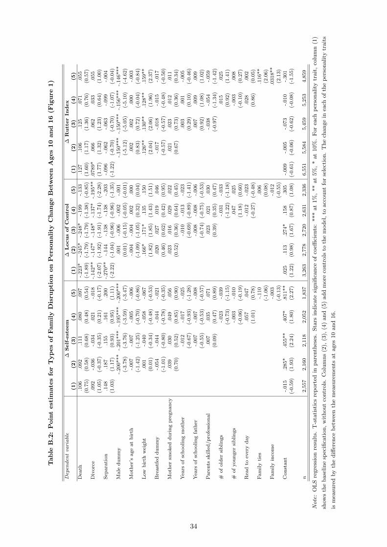
Tab
leB
.2:
Poin
test
imate
sfo
rT
yp
es
of
Fam
ily
Dis
rup
tion
on
Pers
on
ali
tyC
han
ge
Betw
een
Ages
10
an
d16
(Fig
ure
1)
Depen
den
tva
riable
∆Self-esteem
∆LocusofControl
∆RutterIn
dex
(1)
(2)
(3)
(4)
(5)
(1)
(2)
(3)
(4)
(5)
(1)
(2)
(3)
(4)
(5)
Dea
th.1
06
.092
.111
.080
.097
-.223*
-.245*
-.248*
-.199
-.133
.127
.106
.125
.071
.055
(0.7
5)
(0.5
8)
(0.6
8)
(0.4
8)
(0.5
4)
(-1.8
9)
(-1.7
9)
(-1.7
9)
(-1.3
8)
(-0.8
5)
(1.6
0)
(1.1
7)
(1.3
6)
(0.7
6)
(0.5
7)
Div
orc
e.0
92
-.036
-.034
.021
-.018
-.142**
-.147*
-.148*
-.137*
-.195**
.0789*
.066
.062
.033
.055
(1.0
5)
(-0.3
7)
(-0.3
5)
(0.2
1)
(-0.1
7)
(-2.0
7)
(-1.9
2)
(-1.9
1)
(-1.7
4)
(-2.2
8)
(1.7
7)
(1.3
2)
(1.2
3)
(0.6
4)
(1.0
0)
Sep
ara
tion
.148
.187
.155
.161
.200
-.270**
-.144
-.138
-.138
-.203
-.096
-.062
-.063
-.099
-.004
(1.0
3)
(1.1
7)
(0.9
3)
(0.9
5)
(1.1
1)
(-2.2
2)
(-1.0
4)
(-0.9
6)
(-0.9
6)
(-1.3
5)
(-1.2
2)
(-0.7
0)
(-0.7
0)
(-1.0
7)
(-0.0
4)
Male
du
mm
y-.
200***
-.201***
-.195***
-.200***
.001
-.006
-.002
-.001
-.150***
-.150***
-.156***
-.146***
(-3.7
8)
(-3.7
6)
(-3.5
9)
(-3.4
7)
(0.0
1)
(-0.1
5)
(-0.0
5)
(-0.0
1)
(-5.1
2)
(-5.0
5)
(-5.1
0)
(-4.6
2)
Moth
er’s
age
at
bir
th-.
007
-.007
-.005
-.006
-.004
-.004
.002
.000
.002
.002
.000
-.003
(-1.4
2)
(-1.2
5)
(-0.7
0)
(-0.8
6)
(-1.0
9)
(-1.0
5)
(0.3
2)
(0.0
4)
(0.8
3)
(0.7
2)
(-0.0
4)
(-0.8
4)
Low
bir
thw
eight
.001
-.040
-.058
-.067
.166*
.171*
.135
.150
.126**
.130**
.128**
.159**
(0.0
1)
(-0.3
4)
(-0.4
8)
(-0.5
3)
(1.8
2)
(1.8
5)
(1.4
3)
(1.5
1)
(2.0
4)
(2.0
6)
(1.9
6)
(2.3
7)
Bre
ast
fed
du
mm
y-.
054
-.044
-.044
-.021
.020
.027
.019
.046
-.017
-.018
-.015
-.017
(-1.0
1)
(-0.8
0)
(-0.7
8)
(-0.3
5)
(0.4
6)
(0.6
2)
(0.4
2)
(0.9
5)
(-0.5
7)
(-0.5
7)
(-0.4
8)
(-0.5
0)
Moth
ersm
oked
du
rin
gp
regn
an
cy.0
39
.030
.049
.056
.023
.016
.029
.022
.021
.023
.012
.011
(0.7
0)
(0.5
2)
(0.8
5)
(0.9
0)
(0.5
2)
(0.3
6)
(0.6
4)
(0.4
5)
(0.6
7)
(0.7
3)
(0.3
6)
(0.3
4)
Yea
rsof
sch
oolin
gm
oth
er-.
012
-.017
-.025
-.010
-.013
-.023
.003
.001
-.005
(-0.6
7)
(-0.9
3)
(-1.2
8)
(-0.6
9)
(-0.8
9)
(-1.4
1)
(0.2
9)
(0.1
0)
(-0.4
6)
Yea
rsof
sch
oolin
gfa
ther
-.007
-.007
-.008
-.008
-.008
-.006
.007
.009
.009
(-0.5
5)
(-0.5
3)
(-0.5
7)
(-0.7
4)
(-0.7
5)
(-0.5
3)
(0.9
2)
(1.0
8)
(1.0
2)
Pare
nts
skille
d/p
rofe
ssio
nal
.007
.035
.071
.023
.021
.030
-.038
-.054
-.059
(0.0
9)
(0.4
7)
(0.8
9)
(0.3
9)
(0.3
5)
(0.4
7)
(-0.9
7)
(-1.3
4)
(-1.4
2)
#of
old
ersi
blin
gs
-.023
-.039
-.031
-.033
.015
.025
(-0.7
3)
(-1.1
5)
(-1.2
2)
(-1.1
8)
(0.9
2)
(1.4
1)
#of
you
nger
sib
lin
gs
-.003
-.010
.047
.025
-.003
.008
(-0.0
6)
(-0.1
9)
(1.1
8)
(0.6
0)
(-0.1
0)
(0.2
7)
Rea
dto
ever
yd
ay
.057
.047
-.012
-.023
.028
.002
(1.0
1)
(0.7
8)
(-0.2
7)
(-0.4
8)
(0.8
6)
(0.0
5)
Fam
ily
ties
-.110
.006
.116**
(-1.0
6)
(0.0
8)
(2.0
6)
Fam
ily
inco
me
-.003
-.012
.0318**
(-0.1
3)
(-0.5
5)
(2.1
3)
Con
stant
-.015
.285*
.455**
.407*
.811**
.025
.113
.274*
.158
.305
-.009
-.005
-.073
-.010
-.301
(-0.5
9)
(1.9
3)
(2.2
4)
(1.8
0)
(2.2
7)
(1.2
2)
(0.9
8)
(1.6
7)
(0.8
7)
(1.0
8)
(-0.6
1)
(-0.0
6)
(-0.6
2)
(-0.0
8)
(-1.5
5)
n2,5
57
2,1
60
2,1
18
2,0
52
1,8
37
3,2
63
2,7
78
2,7
20
2,6
31
2,3
36
6,5
51
5,5
84
5,4
59
5,2
53
4,8
59
Note:
OL
Sre
gre
ssio
nre
sult
s.T
-sta
tist
ics
rep
ort
edin
pare
nth
eses
.Sta
rsin
dic
ate
signifi
cance
of
coeffi
cien
ts:
***
at
1%
,**
at
5%
,*
at
10%
.F
or
each
per
sonality
trait
,co
lum
n(1
)
show
sth
ebase
line
spec
ifica
tion,
wit
hout
contr
ols
.C
olu
mns
(2),
(3),
(4)
and
(5)
add
more
contr
ols
toth
em
odel
,to
acc
ount
for
sele
ctio
n.
The
change
inea
chof
the
per
sonality
trait
s
ism
easu
red
by
the
diff
eren
ceb
etw
een
the
mea
sure
men
tsat
ages
10
and
16.
34
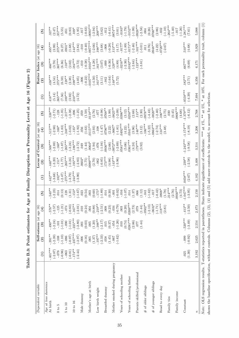
Tab
leB
.3:
Poin
test
imate
sfo
rA
ge
at
Fam
ily
Dis
rupti
on
on
Pers
on
ali
tyL
evel
at
Age
16
(Fig
ure
2)
Depen
den
tva
riable
Self-esteem
(at
age
16)
LocusofControl
(at
age
16)
RutterIn
dex
(at
age
16)
(1)
(2)
(3)
(4)
(5)
(1)
(2)
(3)
(4)
(5)
(1)
(2)
(3)
(4)
(5)
Age
atloss
dummies
At
bir
th-.
401***
-.391**
-.490**
-.576**
-.540**
-.442***
-.440***
-.508***
-.515***
-.538***
.418***
.438***
.466***
.495***
.337**
(-2.8
7)
(-2.3
9)
(-2.2
4)
(-2.5
7)
(-2.2
3)
(-3.6
8)
(-3.2
0)
(-2.8
9)
(-2.9
0)
(-2.7
1)
(5.1
4)
(4.5
4)
(3.7
8)
(3.9
9)
(2.4
7)
0to
5-.
078
-.108
-.101
-.125
.014
-.182**
-.151*
-.160*
-.160*
-.128
.365***
.375***
.367***
.375***
.357***
(-0.9
6)
(-1.1
0)
(-1.0
1)
(-1.2
1)
(0.1
3)
(-2.4
7)
(-1.7
7)
(-1.8
7)
(-1.8
3)
(-1.3
5)
(7.5
6)
(6.5
9)
(6.3
6)
(6.2
7)
(5.5
5)
5to
10
-.063
-.086
-.090
-.074
.128
-.275***
-.265***
-.265***
-.248***
-.217**
.189***
.128**
.110**
.0931*
.051
(-0.8
1)
(-0.9
7)
(-1.0
1)
(-0.8
3)
(1.3
1)
(-3.7
9)
(-3.2
4)
(-3.2
4)
(-3.0
2)
(-2.3
8)
(3.9
2)
(2.3
8)
(2.0
2)
(1.6
8)
(0.8
3)
10
to16
-.174**
-.237***
-.225***
-.167**
-.153*
-.244***
-.195***
-.186***
-.135*
-.096
.210***
.198***
.184***
.144***
.109*
(-2.4
4)
(-2.9
7)
(-2.8
0)
(-2.0
1)
(-1.6
7)
(-3.9
0)
(-2.8
3)
(-2.7
2)
(-1.9
2)
(-1.2
5)
(4.7
2)
(4.0
5)
(3.7
2)
(2.8
4)
(1.9
5)
Male
du
mm
y.0
06
.001
.010
.023
.0602*
.049
.056
.059
-.006
-.010
-.010
-.017
(0.1
6)
(0.0
3)
(0.2
4)
(0.5
4)
(1.7
5)
(1.4
4)
(1.6
3)
(1.5
9)
(-0.2
2)
(-0.3
8)
(-0.4
0)
(-0.6
3)
Moth
er’s
age
at
bir
th.0
05
.005
.004
.003
.0089***
.0064*
.0115***
.0118***
-.0107***
-.0104***
-.0077***
-.0093***
(1.3
7)
(1.2
0)
(0.8
8)
(0.6
0)
(2.7
0)
(1.9
4)
(2.9
3)
(2.7
6)
(-4.5
0)
(-4.2
8)
(-2.6
6)
(-2.9
4)
Low
bir
thw
eight
-.197**
-.188**
-.219**
-.175*
-.062
-.076
-.108
-.077
.161***
.161***
.198***
.209***
(-2.3
3)
(-2.1
7)
(-2.5
1)
(-1.8
9)
(-0.8
5)
(-1.0
4)
(-1.4
7)
(-0.9
8)
(3.1
1)
(3.0
7)
(3.6
8)
(3.6
2)
Bre
ast
fed
du
mm
y.0
58
.015
.009
.014
.173***
.0936***
.0796**
.0768**
-.042
-.009
-.008
-.012
(1.4
5)
(0.3
7)
(0.2
3)
(0.3
0)
(4.9
8)
(2.6
6)
(2.2
2)
(1.9
9)
(-1.6
4)
(-0.3
6)
(-0.2
8)
(-0.4
1)
Moth
ersm
oked
du
rin
gp
regn
an
cy-.
067
-.054
-.034
-.001
-.143***
-.0972***
-.0667*
-.0825**
.148***
.129***
.113***
.0874***
(-1.6
2)
(-1.2
6)
(-0.7
9)
(-0.0
2)
(-3.9
6)
(-2.6
9)
(-1.8
1)
(-2.0
9)
(5.7
2)
(4.8
9)
(4.1
7)
(3.0
1)
Yea
rsof
sch
oolin
gm
oth
er.0
10
.003
-.016
.0581***
.0492***
.0396***
-.0216**
-.0177*
-.0183*
(0.7
4)
(0.2
0)
(-1.0
7)
(5.0
6)
(4.2
2)
(3.1
2)
(-2.3
6)
(-1.8
9)
(-1.7
9)
Yea
rsof
sch
oolin
gfa
ther
.0281***
.0269***
.014
.0361***
.0341***
.0250***
-.0182***
-.0171**
-.0152**
(2.8
6)
(2.7
3)
(1.3
7)
(4.2
4)
(3.9
6)
(2.6
8)
(-2.6
4)
(-2.4
6)
(-1.9
9)
Pare
nts
skille
d/p
rofe
ssio
nal
.077
.079
.066
.179***
.146***
.115**
-.123***
-.101***
-.0928***
(1.4
4)
(1.4
4)
(1.1
2)
(3.9
2)
(3.1
2)
(2.3
0)
(-3.8
1)
(-3.0
1)
(-2.5
8)
#of
old
ersi
blin
gs
-.0502**
-.041
-.106***
-.0978***
.011
.004
(-2.1
3)
(-1.6
2)
(-5.2
2)
(-4.4
3)
(0.7
6)
(0.2
6)
#of
you
nger
sib
lin
gs
-.0632*
-.017
-.0863***
-.0820**
.0948***
.0700***
(-1.7
1)
(-0.4
2)
(-2.7
4)
(-2.4
0)
(4.2
2)
(2.8
6)
Rea
dto
ever
yd
ay
.118***
.0808*
.124***
.106***
-.0720***
-.032
(2.8
1)
(1.7
8)
(3.4
8)
(2.7
5)
(-2.6
7)
(-1.1
0)
Fam
ily
ties
.214***
.030
-.264***
(2.7
6)
(0.4
5)
(-5.4
0)
Fam
ily
inco
me
.0930***
.0806***
-.017
(4.7
3)
(4.6
8)
(-1.2
6)
Con
stant
.025
-.099
-.520***
-.413**
-1.0
47***
.0458***
-.239**
-1.2
43***
-1.1
74***
-1.3
79***
-.0559***
.182***
.667***
.510***
1.2
81***
(1.3
0)
(-0.9
2)
(-3.4
9)
(-2.5
0)
(-3.9
5)
(2.6
7)
(-2.5
8)
(-9.5
8)
(-8.1
9)
(-6.1
2)
(-4.3
9)
(2.7
1)
(6.6
9)
(4.6
8)
(7.6
1)
n3,1
92
2,6
25
2,5
54
2,4
73
2,1
50
4,1
02
3,4
08
3,3
14
3,2
06
2,7
68
7,6
94
6,3
56
6,1
71
5,9
29
5,0
88
Note:
OL
Sre
gre
ssio
nre
sult
s.T
-sta
tist
ics
rep
ort
edin
pare
nth
eses
.Sta
rsin
dic
ate
signifi
cance
of
coeffi
cien
ts:
***
at
1%
,**
at
5%
,*
at
10%
.F
or
each
per
sonality
trait
,co
lum
n(1
)
show
sth
ebase
line
spec
ifica
tion,
wit
hout
contr
ols
.C
olu
mns
(2),
(3),
(4)
and
(5)
add
more
contr
ols
toth
em
odel
,to
acc
ount
for
sele
ctio
n.
35

Tab
leB
.4:
Poin
test
imate
sfo
rA
ge
at
Fam
ily
Dis
rup
tion
on
Pers
on
ali
tyC
han
ge
Betw
een
Ages
10
an
d16
(Fig
ure
2)
Depen
den
tva
riable
∆Self-esteem
∆LocusofControl
∆RutterIn
dex
(1)
(2)
(3)
(4)
(5)
(1)
(2)
(3)
(4)
(5)
(1)
(2)
(3)
(4)
(5)
Age
atloss
dummies
At
bir
th-.
187
-.419*
-.644**
-.693**
-.736**
-.069
-.119
-.292
-.282
-.388
.103
.230**
.400***
.362**
.416***
(-0.9
6)
(-1.9
3)
(-2.2
3)
(-2.3
3)
(-2.3
0)
(-0.4
5)
(-0.6
9)
(-1.3
0)
(-1.2
3)
(-1.6
1)
(1.0
6)
(1.9
8)
(2.6
7)
(2.3
8)
(2.6
6)
0to
5.2
42**
.202
.193
.182
.198
-.023
-.020
-.021
-.012
-.105
.168***
.191***
.186***
.178**
.208***
(2.2
1)
(1.5
4)
(1.4
4)
(1.3
3)
(1.3
4)
(-0.2
6)
(-0.1
9)
(-0.2
0)
(-0.1
1)
(-0.8
9)
(2.9
2)
(2.8
6)
(2.7
3)
(2.5
2)
(2.8
8)
5to
10
.153
.106
.105
.119
.102
-.291***
-.274***
-.266***
-.285***
-.340***
.059
.056
.054
.036
.069
(1.4
5)
(0.9
1)
(0.8
8)
(1.0
0)
(0.8
0)
(-3.3
1)
(-2.7
3)
(-2.6
1)
(-2.8
0)
(-3.0
9)
(1.0
5)
(0.8
8)
(0.8
4)
(0.5
5)
(1.0
0)
10
to16
-.130
-.235**
-.241**
-.206*
-.245**
-.169**
-.155*
-.164*
-.132
-.139
.070
.069
.081
.012
.027
(-1.3
3)
(-2.2
1)
(-2.2
3)
(-1.8
5)
(-1.9
9)
(-2.2
1)
(-1.8
4)
(-1.9
3)
(-1.5
1)
(-1.4
7)
(1.3
3)
(1.2
0)
(1.3
9)
(0.2
0)
(0.4
3)
Male
du
mm
y-.
211***
-.214***
-.210***
-.222***
-.004
-.012
-.006
-.006
-.149***
-.151***
-.157***
-.146***
(-4.0
8)
(-4.0
7)
(-3.9
3)
(-3.9
0)
(-0.0
9)
(-0.2
8)
(-0.1
4)
(-0.1
4)
(-5.2
0)
(-5.1
7)
(-5.2
2)
(-4.7
1)
Moth
er’s
age
at
bir
th-.
007
-.007
-.006
-.007
-.005
-.005
.002
.000
.003
.002
-.001
-.004
(-1.4
8)
(-1.2
9)
(-0.9
3)
(-1.1
0)
(-1.3
2)
(-1.2
8)
(0.3
1)
(0.0
4)
(1.0
6)
(0.7
9)
(-0.2
4)
(-1.0
2)
Low
bir
thw
eight
-.026
-.060
-.073
-.085
.150*
.150*
.115
.127
.140**
.137**
.136**
.168**
(-0.2
3)
(-0.5
2)
(-0.6
2)
(-0.6
9)
(1.6
9)
(1.6
6)
(1.2
5)
(1.3
2)
(2.3
2)
(2.2
1)
(2.1
4)
(2.5
6)
Bre
ast
fed
du
mm
y-.
044
-.033
-.032
-.019
.019
.028
.020
.038
-.011
-.012
-.010
-.011
(-0.8
4)
(-0.6
0)
(-0.5
7)
(-0.3
1)
(0.4
5)
(0.6
4)
(0.4
5)
(0.8
1)
(-0.3
7)
(-0.3
9)
(-0.3
3)
(-0.3
4)
Moth
ersm
oked
du
rin
gp
regn
an
cy.0
49
.035
.051
.066
.024
.016
.027
.024
.019
.021
.012
.013
(0.8
9)
(0.6
2)
(0.8
9)
(1.0
8)
(0.5
6)
(0.3
5)
(0.6
0)
(0.5
0)
(0.6
4)
(0.6
8)
(0.3
9)
(0.4
1)
Yea
rsof
sch
oolin
gm
oth
er-.
017
-.022
-.031
-.012
-.017
-.023
.003
.001
-.004
(-0.9
9)
(-1.2
4)
(-1.6
0)
(-0.8
4)
(-1.1
4)
(-1.4
4)
(0.3
0)
(0.1
0)
(-0.3
9)
Yea
rsof
sch
oolin
gfa
ther
-.004
-.004
-.007
-.008
-.007
-.005
.007
.008
.009
(-0.3
3)
(-0.2
9)
(-0.5
1)
(-0.7
1)
(-0.6
5)
(-0.4
0)
(0.8
7)
(1.0
1)
(1.0
0)
Pare
nts
skille
d/p
rofe
ssio
nal
.005
.036
.069
.019
.020
.021
-.044
-.058
-.064
(0.0
7)
(0.4
9)
(0.8
9)
(0.3
4)
(0.3
5)
(0.3
4)
(-1.1
7)
(-1.4
8)
(-1.5
6)
#of
old
ersi
blin
gs
-.018
-.028
-.031
-.029
.017
.027
(-0.5
8)
(-0.8
5)
(-1.2
3)
(-1.0
9)
(1.0
7)
(1.5
5)
#of
you
nger
sib
lin
gs
-.009
-.003
.055
.034
-.007
.003
(-0.1
8)
(-0.0
7)
(1.4
1)
(0.8
2)
(-0.2
7)
(0.1
2)
Rea
dto
ever
yd
ay
.054
.050
-.014
-.025
.042
.014
(0.9
6)
(0.8
3)
(-0.3
3)
(-0.5
3)
(1.3
2)
(0.4
3)
Fam
ily
ties
-.088
.011
.133**
(-0.8
7)
(0.1
3)
(2.4
2)
Fam
ily
inco
me
.009
-.013
.0279*
(0.3
6)
(-0.6
2)
(1.8
9)
Con
stant
-.009
.297**
.492**
.473**
.797**
.027
.139
.320**
.187
.298
-.020
-.036
-.083
-.003
-.338*
(-0.3
5)
(2.0
7)
(2.4
6)
(2.1
3)
(2.2
7)
(1.3
1)
(1.2
3)
(1.9
8)
(1.0
5)
(1.0
8)
(-1.3
3)
(-0.4
6)
(-0.7
1)
(-0.0
2)
(-1.7
8)
n2,6
71
2,2
44
2,1
87
2,1
18
1,8
93
3,3
99
2,8
82
2,8
06
2,7
12
2,4
04
6,8
67
5,8
16
5,6
51
5,4
33
5,0
28
Note:
OL
Sre
gre
ssio
nre
sult
s.T
-sta
tist
ics
rep
ort
edin
pare
nth
eses
.Sta
rsin
dic
ate
signifi
cance
of
coeffi
cien
ts:
***
at
1%
,**
at
5%
,*
at
10%
.F
or
each
per
sonality
trait
,co
lum
n(1
)
show
sth
ebase
line
spec
ifica
tion,
wit
hout
contr
ols
.C
olu
mns
(2),
(3),
(4)
and
(5)
add
more
contr
ols
toth
em
odel
,to
acc
ount
for
sele
ctio
n.
The
change
inea
chof
the
per
sonality
trait
s
ism
easu
red
by
the
diff
eren
ceb
etw
een
the
mea
sure
men
tsat
ages
10
and
16.
36
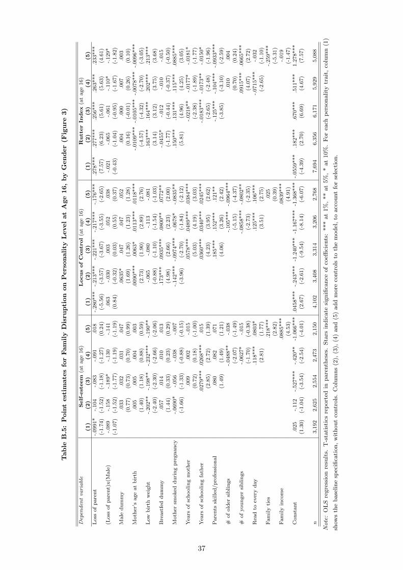
Tab
leB
.5:
Poin
test
imate
sfo
rFam
ily
Dis
rup
tion
on
Pers
on
ali
tyL
evel
at
Age
16,
by
Gen
der
(Fig
ure
3)
Depen
den
tva
riable
Self-esteem
(at
age
16)
LocusofControl
(at
age
16)
RutterIn
dex
(at
age
16)
(1)
(2)
(3)
(4)
(5)
(1)
(2)
(3)
(4)
(5)
(1)
(2)
(3)
(4)
(5)
Loss
of
pare
nt
-.0991*
-.104
-.083
-.091
.018
-.280***
-.213***
-.221***
-.217***
-.176***
.278***
.277***
.256***
.263***
.233***
(-1.7
4)
(-1.5
2)
(-1.1
8)
(-1.2
7)
(0.2
4)
(-5.5
6)
(-3.5
7)
(-3.6
7)
(-3.5
5)
(-2.6
5)
(7.5
7)
(6.2
3)
(5.6
1)
(5.6
3)
(4.6
1)
(Loss
of
pare
nt)
x(M
ale
)-.
089
-.158
-.189*
-.130
-.141
.063
-.030
.003
.052
.038
-.021
-.065
-.061
-.110*
-.129*
(-1.0
7)
(-1.5
2)
(-1.7
7)
(-1.1
9)
(-1.1
9)
(0.8
4)
(-0.3
2)
(0.0
3)
(0.5
5)
(0.3
7)
(-0.4
3)
(-1.0
4)
(-0.9
5)
(-1.6
7)
(-1.8
2)
Male
du
mm
y.0
33
.032
.031
.047
.0635*
.047
.047
.052
.004
.000
.007
.003
(0.7
7)
(0.7
3)
(0.7
0)
(0.9
9)
(1.6
9)
(1.2
6)
(1.2
3)
(1.2
8)
(0.1
6)
(-0.0
1)
(0.2
6)
(0.1
0)
Moth
er’s
age
at
bir
th.0
05
.005
.004
.003
.0090***
.0063*
.0113***
.0118***
-.0109***
-.0105***
-.0078***
-.0096***
(1.4
0)
(1.1
8)
(0.8
8)
(0.5
9)
(2.7
3)
(1.9
0)
(2.8
9)
(2.7
6)
(-4.5
7)
(-4.3
2)
(-2.7
0)
(-3.0
5)
Low
bir
thw
eight
-.202**
-.198**
-.232***
-.190**
-.065
-.080
-.113
-.081
.163***
.164***
.202***
.213***
(-2.4
0)
(-2.3
0)
(-2.6
6)
(-2.0
6)
(-0.8
8)
(-1.1
0)
(-1.5
4)
(-1.0
3)
(3.1
4)
(3.1
2)
(3.7
5)
(3.6
8)
Bre
ast
fed
du
mm
y.0
57
.014
.010
.013
.173***
.0935***
.0800**
.0772**
-.0455*
-.012
-.010
-.015
(1.4
4)
(0.3
3)
(0.2
3)
(0.2
9)
(4.9
8)
(2.6
6)
(2.2
3)
(2.0
0)
(-1.7
7)
(-0.4
4)
(-0.3
7)
(-0.5
0)
Moth
ersm
oked
du
rin
gp
regn
an
cy-.
0690*
-.056
-.038
-.007
-.142***
-.0974***
-.0678*
-.0835**
.150***
.131***
.115***
.0885***
(-1.6
6)
(-1.3
3)
(-0.8
8)
(-0.1
5)
(-3.9
6)
(-2.7
0)
(-1.8
4)
(-2.1
2)
(5.8
1)
(4.9
6)
(4.2
5)
(3.0
5)
Yea
rsof
sch
oolin
gm
oth
er.0
09
.002
-.015
.0578***
.0489***
.0384***
-.0218**
-.0177*
-.0181*
(0.7
2)
(0.1
8)
(-1.0
0)
(5.0
3)
(4.1
9)
(3.0
3)
(-2.3
8)
(-1.8
9)
(-1.7
7)
Yea
rsof
sch
oolin
gfa
ther
.0279***
.0268***
.015
.0360***
.0340***
.0245***
-.0183***
-.0173**
-.0150*
(2.8
5)
(2.7
2)
(1.3
9)
(4.2
3)
(3.9
5)
(2.6
2)
(-2.6
5)
(-2.4
8)
(-1.9
6)
Pare
nts
skille
d/p
rofe
ssio
nal
.080
.082
.071
.185***
.152***
.121**
-.125***
-.104***
-.0933***
(1.4
9)
(1.4
9)
(1.2
1)
(4.0
6)
(3.2
6)
(2.4
2)
(-3.8
5)
(-3.1
0)
(-2.5
9)
#of
old
ersi
blin
gs
-.0488**
-.038
-.105***
-.0964***
.010
.004
(-2.0
7)
(-1.4
9)
(-5.1
5)
(-4.3
7)
(0.7
0)
(0.2
4)
#of
you
nger
sib
lin
gs
-.0627*
-.015
-.0858***
-.0802**
.0915***
.0665***
(-1.7
0)
(-0.3
8)
(-2.7
3)
(-2.3
5)
(4.0
7)
(2.7
2)
Rea
dto
ever
yd
ay
.118***
.0803*
.125***
.106***
-.0715***
-.032
(2.8
1)
(1.7
7)
(3.5
1)
(2.7
5)
(-2.6
5)
(-1.1
0)
Fam
ily
ties
.218***
.025
-.259***
(2.8
2)
(0.3
9)
(-5.3
1)
Fam
ily
inco
me
.0885***
.0839***
-.019
(4.5
3)
(4.9
1)
(-1.4
7)
Con
stant
.025
-.112
-.527***
-.420**
-1.0
66***
.0458***
-.243***
-1.2
40***
-1.1
67***
-1.3
68***
-.0559***
.182***
.670***
.511***
1.2
78***
(1.3
0)
(-1.0
4)
(-3.5
4)
(-2.5
4)
(-4.0
1)
(2.6
7)
(-2.6
1)
(-9.5
4)
(-8.1
4)
(-6.0
7)
(-4.3
9)
(2.7
0)
(6.6
9)
(4.6
7)
(7.5
7)
n3,1
92
2,6
25
2,5
54
2,4
73
2,1
50
4,1
02
3,4
08
3,3
14
3,2
06
2,7
68
7,6
94
6,3
56
6,1
71
5,9
29
5,0
88
Note:
OL
Sre
gre
ssio
nre
sult
s.T
-sta
tist
ics
rep
ort
edin
pare
nth
eses
.Sta
rsin
dic
ate
signifi
cance
of
coeffi
cien
ts:
***
at
1%
,**
at
5%
,*
at
10%
.F
or
each
per
sonality
trait
,co
lum
n(1
)
show
sth
ebase
line
spec
ifica
tion,
wit
hout
contr
ols
.C
olu
mns
(2),
(3),
(4)
and
(5)
add
more
contr
ols
toth
em
odel
,to
acc
ount
for
sele
ctio
n.
37
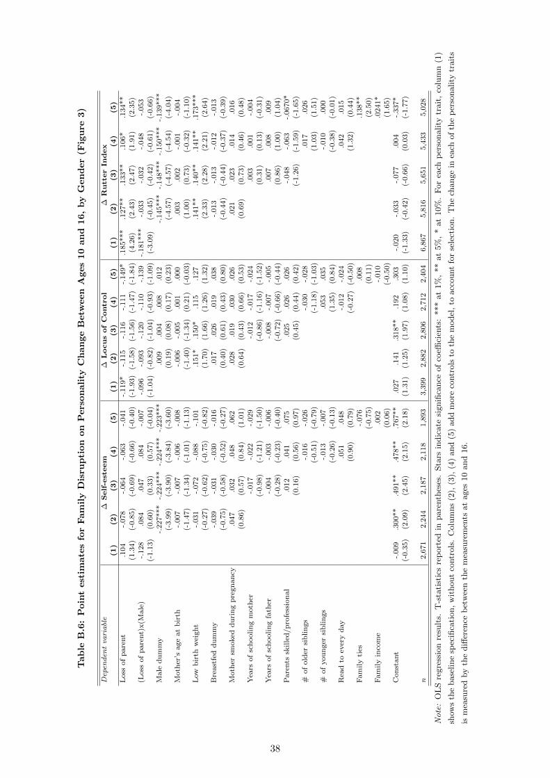
Tab
leB
.6:
Poin
test
imate
sfo
rFam
ily
Dis
rup
tion
on
Pers
on
ali
tyC
han
ge
Betw
een
Ages
10
an
d16,
by
Gen
der
(Fig
ure
3)
Depen
den
tva
riable
∆Self-esteem
∆LocusofControl
∆RutterIn
dex
(1)
(2)
(3)
(4)
(5)
(1)
(2)
(3)
(4)
(5)
(1)
(2)
(3)
(4)
(5)
Loss
of
pare
nt
.104
-.078
-.064
-.063
-.041
-.119*
-.115
-.116
-.111
-.149*
.185***
.127**
.133**
.106*
.134**
(1.3
4)
(-0.8
5)
(-0.6
9)
(-0.6
6)
(-0.4
0)
(-1.9
3)
(-1.5
8)
(-1.5
6)
(-1.4
7)
(-1.8
4)
(4.2
6)
(2.4
3)
(2.4
7)
(1.9
1)
(2.3
5)
(Loss
of
pare
nt)
x(M
ale
)-.
128
.084
.047
.084
-.007
-.096
-.093
-.120
-.110
-.139
-.181***
-.033
-.032
-.048
-.053
(-1.1
3)
(0.6
0)
(0.3
3)
(0.5
7)
(-0.0
4)
(-1.0
4)
(-0.8
2)
(-1.0
4)
(-0.9
3)
(-1.0
9)
(-3.0
9)
(-0.4
5)
(-0.4
2)
(-0.6
1)
(-0.6
6)
Male
du
mm
y-.
227***
-.224***
-.224***
-.223***
.009
.004
.008
.012
-.145***
-.148***
-.150***
-.139***
(-3.9
9)
(-3.9
0)
(-3.8
4)
(-3.6
0)
(0.1
9)
(0.0
8)
(0.1
7)
(0.2
3)
(-4.5
7)
(-4.5
7)
(-4.5
4)
(-4.0
4)
Moth
er’s
age
at
bir
th-.
007
-.007
-.006
-.008
-.006
-.005
.001
.000
.003
.002
-.001
-.004
(-1.4
7)
(-1.3
4)
(-1.0
1)
(-1.1
3)
(-1.4
0)
(-1.3
4)
(0.2
1)
(-0.0
3)
(1.0
0)
(0.7
3)
(-0.3
2)
(-1.1
0)
Low
bir
thw
eight
-.031
-.072
-.088
-.101
.151*
.150*
.115
.127
.141**
.140**
.141**
.173***
(-0.2
7)
(-0.6
2)
(-0.7
5)
(-0.8
2)
(1.7
0)
(1.6
6)
(1.2
6)
(1.3
2)
(2.3
3)
(2.2
8)
(2.2
1)
(2.6
4)
Bre
ast
fed
du
mm
y-.
039
-.031
-.030
-.016
.017
.026
.019
.038
-.013
-.013
-.012
-.013
(-0.7
5)
(-0.5
8)
(-0.5
2)
(-0.2
7)
(0.4
0)
(0.6
1)
(0.4
3)
(0.8
0)
(-0.4
4)
(-0.4
4)
(-0.3
7)
(-0.3
9)
Moth
ersm
oked
du
rin
gp
regn
an
cy.0
47
.032
.048
.062
.028
.019
.030
.026
.021
.023
.014
.016
(0.8
6)
(0.5
7)
(0.8
4)
(1.0
1)
(0.6
4)
(0.4
3)
(0.6
6)
(0.5
3)
(0.6
9)
(0.7
3)
(0.4
6)
(0.4
8)
Yea
rsof
sch
oolin
gm
oth
er-.
017
-.022
-.029
-.012
-.017
-.024
.003
.001
-.004
(-0.9
8)
(-1.2
1)
(-1.5
0)
(-0.8
6)
(-1.1
6)
(-1.5
2)
(0.3
1)
(0.1
3)
(-0.3
1)
Yea
rsof
sch
oolin
gfa
ther
-.004
-.003
-.006
-.008
-.007
-.005
.007
.008
.009
(-0.2
8)
(-0.2
3)
(-0.4
0)
(-0.7
2)
(-0.6
6)
(-0.4
4)
(0.8
6)
(1.0
0)
(1.0
4)
Pare
nts
skille
d/p
rofe
ssio
nal
.012
.041
.075
.025
.026
.026
-.048
-.063
-.0670*
(0.1
6)
(0.5
6)
(0.9
7)
(0.4
5)
(0.4
4)
(0.4
2)
(-1.2
6)
(-1.5
9)
(-1.6
5)
#of
old
ersi
bli
ngs
-.016
-.026
-.030
-.028
.017
.026
(-0.5
1)
(-0.7
9)
(-1.1
8)
(-1.0
3)
(1.0
3)
(1.5
1)
#of
you
nger
sib
lin
gs
-.013
-.007
.053
.035
-.010
.000
(-0.2
6)
(-0.1
3)
(1.3
5)
(0.8
4)
(-0.3
8)
(-0.0
1)
Rea
dto
ever
yd
ay
.051
.048
-.012
-.024
.042
.015
(0.9
0)
(0.7
9)
(-0.2
7)
(-0.5
0)
(1.3
2)
(0.4
4)
Fam
ily
ties
-.076
.008
.138**
(-0.7
5)
(0.1
1)
(2.5
0)
Fam
ily
inco
me
.002
-.010
.0241*
(0.0
6)
(-0.5
0)
(1.6
5)
Con
stant
-.009
.300**
.491**
.478**
.767**
.027
.141
.318**
.192
.303
-.020
-.033
-.077
.004
-.337*
(-0.3
5)
(2.0
9)
(2.4
5)
(2.1
5)
(2.1
8)
(1.3
1)
(1.2
5)
(1.9
7)
(1.0
8)
(1.1
0)
(-1.3
3)
(-0.4
2)
(-0.6
6)
(0.0
3)
(-1.7
7)
n2,6
71
2,2
44
2,1
87
2,1
18
1,8
93
3,3
99
2,8
82
2,8
06
2,7
12
2,4
04
6,8
67
5,8
16
5,6
51
5,4
33
5,0
28
Note:
OL
Sre
gre
ssio
nre
sult
s.T
-sta
tist
ics
rep
ort
edin
pare
nth
eses
.Sta
rsin
dic
ate
signifi
cance
of
coeffi
cien
ts:
***
at
1%
,**
at
5%
,*
at
10%
.F
or
each
per
sonality
trait
,co
lum
n(1
)
show
sth
ebase
line
spec
ifica
tion,
wit
hout
contr
ols
.C
olu
mns
(2),
(3),
(4)
and
(5)
add
more
contr
ols
toth
em
odel
,to
acc
ount
for
sele
ctio
n.
The
change
inea
chof
the
per
sonality
trait
s
ism
easu
red
by
the
diff
eren
ceb
etw
een
the
mea
sure
men
tsat
ages
10
and
16.
38

Tab
leB
.7:
Poin
test
imate
sfo
rT
yp
es
of
Fam
ily
Dis
rup
tion
on
Pers
on
ali
tyL
evel
at
Age
16,
by
Gen
der
(Fig
ure
4)
Depen
den
tva
riable
Self-esteem
(at
age
16)
LocusofControl
(at
age
16)
RutterIn
dex
(at
age
16)
(1)
(2)
(3)
(4)
(5)
(1)
(2)
(3)
(4)
(5)
(1)
(2)
(3)
(4)
(5)
Dea
th.1
18
.157
.185
.203
.274
-.049
-.109
-.092
-.088
-.038
-.008
-.020
-.027
-.100
-.121
(0.9
2)
(0.9
8)
(1.1
4)
(1.2
4)
(1.6
1)
(-0.4
2)
(-0.7
4)
(-0.6
4)
(-0.5
9)
(-0.2
5)
(-0.0
9)
(-0.1
8)
(-0.2
4)
(-0.8
9)
(-1.0
3)
Div
orc
e-.
156*
-.173*
-.167*
-.181*
-.083
-.359***
-.243***
-.254***
-.250***
-.182**
.297***
.292***
.276***
.294***
.285***
(-1.9
1)
(-1.8
4)
(-1.7
8)
(-1.8
7)
(-0.7
9)
(-5.0
8)
(-3.0
2)
(-3.1
8)
(-3.0
7)
(-2.0
3)
(5.9
0)
(5.0
2)
(4.6
9)
(4.9
0)
(4.3
3)
Sep
ara
tion
-.039
.045
.074
.083
.141
-.263**
-.156
-.145
-.118
-.116
.301***
.225**
.189**
.199**
.187*
(-0.3
2)
(0.3
3)
(0.5
2)
(0.5
8)
(0.9
3)
(-2.3
1)
(-1.2
2)
(-1.1
3)
(-0.9
2)
(-0.8
5)
(3.6
5)
(2.4
2)
(2.0
1)
(2.0
8)
(1.8
6)
(Dea
th)x
(Male
)-.
556***
-.586**
-.561**
-.598**
-.687**
-.119
-.046
.024
.093
.089
.276**
.298*
.289*
.306*
.288*
(-2.5
9)
(-2.4
2)
(-2.2
9)
(-2.3
8)
(-2.5
2)
(-0.6
1)
(-0.2
1)
(0.1
1)
(0.4
1)
(0.3
6)
(2.0
4)
(1.9
2)
(1.8
5)
(1.9
2)
(1.6
8)
(Div
orc
e)x(M
ale
)-.
042
-.143
-.137
.025
.037
.133
.012
.028
.098
.065
-.020
-.098
-.091
-.162*
-.224**
(-0.3
3)
(-0.9
6)
(-0.9
2)
(0.1
6)
(0.2
2)
(1.1
9)
(0.0
9)
(0.2
2)
(0.7
6)
(0.4
6)
(-0.2
7)
(-1.1
3)
(-1.0
4)
(-1.8
1)
(-2.3
0)
(Sep
ara
tion
)x(M
ale
).1
12
.166
.133
.113
.261
.177
.094
.000
-.012
.076
-.195**
-.203*
-.193*
-.229**
-.254**
(0.7
0)
(0.9
0)
(0.7
0)
(0.5
9)
(1.2
5)
(1.1
7)
(0.5
4)
(0.0
0)
(-0.0
7)
(0.4
0)
(-2.0
8)
(-1.9
0)
(-1.7
9)
(-2.0
8)
(-2.1
7)
Male
du
mm
y.0
33
.032
.031
.046
.0639*
.047
.047
.052
.004
.000
.008
.003
(0.7
8)
(0.7
3)
(0.7
0)
(0.9
9)
(1.7
0)
(1.2
5)
(1.2
3)
(1.2
9)
(0.1
6)
(-0.0
2)
(0.2
7)
(0.0
9)
Moth
er’s
age
at
bir
th.0
05
.004
.004
.003
.0083**
0.0
051
.0102**
.0108**
-.0118***
-.0112***
-.0074**
-.0082**
(1.3
8)
(1.0
9)
(0.8
8)
(0.6
7)
(2.4
4)
(1.5
1)
(2.5
1)
(2.4
7)
(-4.7
9)
(-4.4
6)
(-2.4
8)
(-2.5
3)
Low
bir
thw
eight
-.176**
-.173*
-.209**
-.164*
-.046
-.063
-.094
-.071
.171***
.169***
.210***
.221***
(-2.0
3)
(-1.9
5)
(-2.3
2)
(-1.7
2)
(-0.6
1)
(-0.8
4)
(-1.2
5)
(-0.8
8)
(3.2
0)
(3.1
5)
(3.7
8)
(3.7
3)
Bre
ast
fed
du
mm
y.0
43
.003
.000
.002
.171***
.0821**
.0694*
.0719*
-.0469*
-.015
-.014
-.018
(1.0
5)
(0.0
8)
(-0.0
0)
(0.0
5)
(4.8
4)
(2.2
9)
(1.9
0)
(1.8
4)
(-1.7
9)
(-0.5
6)
(-0.5
1)
(-0.6
0)
Moth
ersm
oked
du
rin
gp
regn
an
cy-.
0760*
-.057
-.036
-.011
-.154***
-.102***
-.0719*
-.0957**
.157***
.140***
.121***
.0895***
(-1.7
9)
(-1.3
3)
(-0.8
1)
(-0.2
4)
(-4.1
7)
(-2.7
6)
(-1.9
2)
(-2.3
9)
(5.9
2)
(5.1
8)
(4.3
9)
(3.0
2)
Yea
rsof
sch
oolin
gm
oth
er.0
11
.004
-.013
.0604***
.0525***
.0398***
-.0207**
-.0169*
-.0185*
(0.8
2)
(0.3
1)
(-0.9
0)
(5.1
7)
(4.4
3)
(3.0
9)
(-2.2
1)
(-1.7
7)
(-1.7
8)
Yea
rsof
sch
oolin
gfa
ther
.0266***
.0252**
.014
.0390***
.0368***
.0276***
-.0188***
-.0179**
-.0166**
(2.7
0)
(2.5
4)
(1.3
6)
(4.5
4)
(4.2
4)
(2.9
3)
(-2.6
9)
(-2.5
2)
(-2.1
3)
Pare
nts
skille
d/p
rofe
ssio
nal
.086
.087
.076
.187***
.154***
.127**
-.107***
-.0863**
-.0716*
(1.5
6)
(1.5
5)
(1.2
6)
(4.0
1)
(3.2
2)
(2.4
7)
(-3.2
1)
(-2.5
1)
(-1.9
4)
#of
old
ersi
bli
ngs
-.0487**
-.0433*
-.111***
-.104***
.010
.002
(-2.0
3)
(-1.6
8)
(-5.3
3)
(-4.6
3)
(0.6
9)
(0.1
0)
#of
you
nger
sib
lin
gs
-.059
-.016
-.0955***
-.0868**
.102***
.0748***
(-1.5
7)
(-0.4
0)
(-2.9
7)
(-2.5
0)
(4.4
5)
(3.0
0)
Rea
dto
ever
yd
ay
.115***
.0765*
.117***
.100**
-.0757***
-.043
(2.6
9)
(1.6
6)
(3.2
4)
(2.5
5)
(-2.7
5)
(-1.4
3)
Fam
ily
ties
.212***
.029
-.280***
(2.6
9)
(0.4
4)
(-5.6
0)
Fam
ily
inco
me
.0821***
.0782***
-.013
(4.1
2)
(4.4
7)
(-0.9
7)
Con
stant
.017
-.122
-.538***
-.442***
-1.0
49***
.0344**
-.236**
-1.2
75***
-1.1
95***
-1.3
74***
-.0386***
.224***
.683***
.495***
1.2
89***
(0.8
5)
(-1.0
9)
(-3.5
4)
(-2.6
1)
(-3.8
6)
(2.0
0)
(-2.4
5)
(-9.5
8)
(-8.1
4)
(-5.9
7)
(-3.0
2)
(3.2
0)
(6.6
6)
(4.4
3)
(7.4
6)
n3,0
55
2,5
29
2,4
77
2,4
00
2,0
92
3,9
31
3,2
81
3,2
10
3,1
08
2,6
93
7,3
19
6,0
84
5,9
46
5,7
19
4,9
15
Note:
OL
Sre
gre
ssio
nre
sult
s.T
-sta
tist
ics
rep
ort
edin
pare
nth
eses
.Sta
rsin
dic
ate
signifi
cance
of
coeffi
cien
ts:
***
at
1%
,**
at
5%
,*
at
10%
.F
or
each
per
sonality
trait
,co
lum
n(1
)
show
sth
ebase
line
spec
ifica
tion,
wit
hout
contr
ols
.C
olu
mns
(2),
(3),
(4)
and
(5)
add
more
contr
ols
toth
em
odel
,to
acc
ount
for
sele
ctio
n.
39
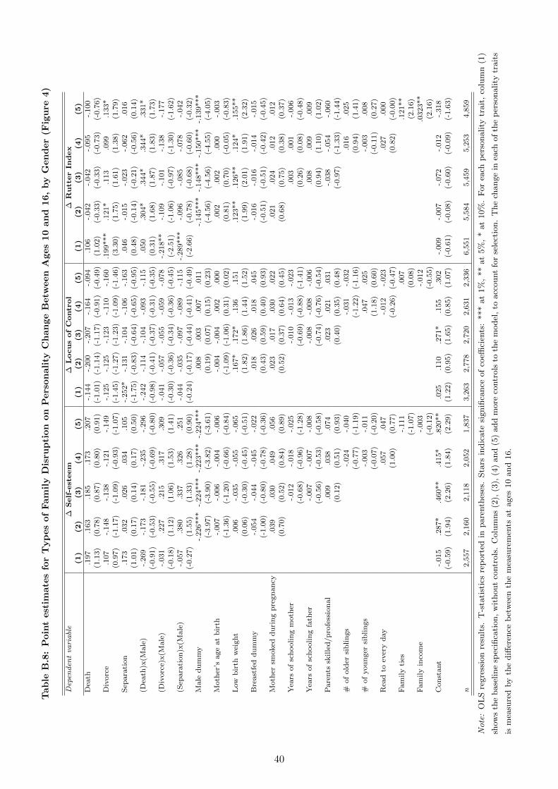
Tab
leB
.8:
Poin
test
imate
sfo
rT
yp
es
of
Fam
ily
Dis
rup
tion
on
Pers
on
ali
tyC
han
ge
Betw
een
Ages
10
an
d16,
by
Gen
der
(Fig
ure
4)
Depen
den
tva
riable
∆Self-esteem
∆LocusofControl
∆RutterIn
dex
(1)
(2)
(3)
(4)
(5)
(1)
(2)
(3)
(4)
(5)
(1)
(2)
(3)
(4)
(5)
Dea
th.1
97
.163
.185
.173
.207
-.144
-.200
-.207
-.164
-.094
.106
-.042
-.042
-.095
-.100
(1.1
3)
(0.7
8)
(0.8
7)
(0.8
0)
(0.9
1)
(-1.0
1)
(-1.1
4)
(-1.1
7)
(-0.9
1)
(-0.4
9)
(1.0
2)
(-0.3
3)
(-0.3
3)
(-0.7
3)
(-0.7
6)
Div
orc
e.1
07
-.148
-.138
-.121
-.149
-.125
-.125
-.123
-.110
-.160
.199***
.121*
.113
.099
.133*
(0.9
7)
(-1.1
7)
(-1.0
9)
(-0.9
3)
(-1.0
7)
(-1.4
5)
(-1.2
7)
(-1.2
3)
(-1.0
9)
(-1.4
6)
(3.3
0)
(1.7
5)
(1.6
1)
(1.3
8)
(1.7
9)
Sep
ara
tion
.173
.032
.026
.034
.105
-.252*
-.131
-.104
-.106
-.163
.046
-.015
-.023
-.062
.016
(1.0
1)
(0.1
7)
(0.1
4)
(0.1
7)
(0.5
0)
(-1.7
5)
(-0.8
3)
(-0.6
4)
(-0.6
5)
(-0.9
5)
(0.4
8)
(-0.1
4)
(-0.2
1)
(-0.5
6)
(0.1
4)
(Dea
th)x
(Male
)-.
269
-.173
-.181
-.235
-.296
-.242
-.114
-.104
-.093
-.115
.050
.304*
.344*
.344*
.331*
(-0.9
1)
(-0.5
3)
(-0.5
5)
(-0.6
9)
(-0.8
0)
(-0.9
8)
(-0.4
1)
(-0.3
7)
(-0.3
1)
(-0.3
5)
(0.3
1)
(1.6
8)
(1.8
7)
(1.8
3)
(1.7
3)
(Div
orc
e)x(M
ale
)-.
031
.227
.215
.317
.309
-.041
-.057
-.055
-.059
-.078
-.218**
-.109
-.101
-.138
-.177
(-0.1
8)
(1.1
2)
(1.0
6)
(1.5
3)
(1.4
1)
(-0.3
0)
(-0.3
6)
(-0.3
4)
(-0.3
6)
(-0.4
5)
(-2.5
1)
(-1.0
6)
(-0.9
7)
(-1.3
0)
(-1.6
2)
(Sep
ara
tion
)x(M
ale
)-.
057
.380
.337
.326
.251
-.044
-.035
-.097
-.089
-.115
-.289***
-.096
-.085
-.078
-.042
(-0.2
7)
(1.5
5)
(1.3
3)
(1.2
8)
(0.9
0)
(-0.2
4)
(-0.1
7)
(-0.4
4)
(-0.4
1)
(-0.4
9)
(-2.6
6)
(-0.7
8)
(-0.6
8)
(-0.6
0)
(-0.3
2)
Male
du
mm
y-.
226***
-.224***
-.223***
-.224***
.008
.003
.007
.011
-.145***
-.148***
-.150***
-.139***
(-3.9
7)
(-3.9
0)
(-3.8
2)
(-3.6
1)
(0.1
9)
(0.0
7)
(0.1
5)
(0.2
3)
(-4.5
6)
(-4.5
6)
(-4.5
5)
(-4.0
5)
Moth
er’s
age
at
bir
th-.
007
-.006
-.004
-.006
-.004
-.004
.002
.000
.002
.002
.000
-.003
(-1.3
6)
(-1.2
0)
(-0.6
6)
(-0.8
4)
(-1.0
9)
(-1.0
6)
(0.3
1)
(0.0
2)
(0.8
1)
(0.7
0)
(-0.0
5)
(-0.8
3)
Low
bir
thw
eight
.006
-.035
-.055
-.065
.167*
.172*
.136
.151
.123**
.126**
.124*
.155**
(0.0
6)
(-0.3
0)
(-0.4
5)
(-0.5
1)
(1.8
2)
(1.8
6)
(1.4
4)
(1.5
2)
(1.9
9)
(2.0
1)
(1.9
1)
(2.3
2)
Bre
ast
fed
du
mm
y-.
054
-.044
-.045
-.022
.018
.026
.018
.045
-.016
-.016
-.014
-.015
(-1.0
0)
(-0.8
0)
(-0.7
8)
(-0.3
6)
(0.4
3)
(0.5
9)
(0.4
0)
(0.9
3)
(-0.5
1)
(-0.5
1)
(-0.4
2)
(-0.4
5)
Moth
ersm
oked
du
rin
gp
regn
an
cy.0
39
.030
.049
.056
.023
.017
.030
.022
.021
.024
.012
.012
(0.7
0)
(0.5
2)
(0.8
4)
(0.8
9)
(0.5
2)
(0.3
7)
(0.6
4)
(0.4
5)
(0.6
8)
(0.7
5)
(0.3
8)
(0.3
7)
Yea
rsof
sch
oolin
gm
oth
er-.
012
-.018
-.025
-.010
-.013
-.023
.003
.001
-.006
(-0.6
8)
(-0.9
6)
(-1.2
8)
(-0.6
9)
(-0.8
8)
(-1.4
1)
(0.2
6)
(0.0
8)
(-0.4
8)
Yea
rsof
sch
oolin
gfa
ther
-.007
-.007
-.008
-.008
-.008
-.006
.008
.009
.009
(-0.5
6)
(-0.5
3)
(-0.5
8)
(-0.7
4)
(-0.7
6)
(-0.5
4)
(0.9
4)
(1.1
0)
(1.0
2)
Pare
nts
skille
d/p
rofe
ssio
nal
.009
.038
.074
.023
.021
.031
-.038
-.054
-.060
(0.1
2)
(0.5
1)
(0.9
3)
(0.4
0)
(0.3
5)
(0.4
8)
(-0.9
7)
(-1.3
3)
(-1.4
4)
#of
old
ersi
bli
ngs
-.024
-.040
-.031
-.032
.016
.025
(-0.7
7)
(-1.1
9)
(-1.2
2)
(-1.1
6)
(0.9
4)
(1.4
1)
#of
you
nger
sib
lin
gs
-.003
-.011
.047
.025
-.003
.008
(-0.0
7)
(-0.2
0)
(1.1
8)
(0.6
0)
(-0.1
1)
(0.2
7)
Rea
dto
ever
yd
ay
.057
.047
-.012
-.023
.027
.000
(1.0
0)
(0.7
7)
(-0.2
6)
(-0.4
7)
(0.8
2)
(-0.0
0)
Fam
ily
ties
-.111
.007
.121**
(-1.0
7)
(0.0
8)
(2.1
6)
Fam
ily
inco
me
-.003
-.012
.0323**
(-0.1
2)
(-0.5
5)
(2.1
6)
Con
stant
-.015
.287*
.460**
.415*
.820**
.025
.110
.271*
.155
.302
-.009
-.007
-.072
-.012
-.318
(-0.5
9)
(1.9
4)
(2.2
6)
(1.8
4)
(2.2
9)
(1.2
2)
(0.9
5)
(1.6
5)
(0.8
5)
(1.0
7)
(-0.6
1)
(-0.0
8)
(-0.6
0)
(-0.0
9)
(-1.6
3)
n2,5
57
2,1
60
2,1
18
2,0
52
1,8
37
3,2
63
2,7
78
2,7
20
2,6
31
2,3
36
6,5
51
5,5
84
5,4
59
5,2
53
4,8
59
Note:
OL
Sre
gre
ssio
nre
sult
s.T
-sta
tist
ics
rep
ort
edin
pare
nth
eses
.Sta
rsin
dic
ate
signifi
cance
of
coeffi
cien
ts:
***
at
1%
,**
at
5%
,*
at
10%
.F
or
each
per
sonality
trait
,co
lum
n(1
)
show
sth
ebase
line
spec
ifica
tion,
wit
hout
contr
ols
.C
olu
mns
(2),
(3),
(4)
and
(5)
add
more
contr
ols
toth
em
odel
,to
acc
ount
for
sele
ctio
n.
The
change
inea
chof
the
per
sonality
trait
s
ism
easu
red
by
the
diff
eren
ceb
etw
een
the
mea
sure
men
tsat
ages
10
and
16.
40
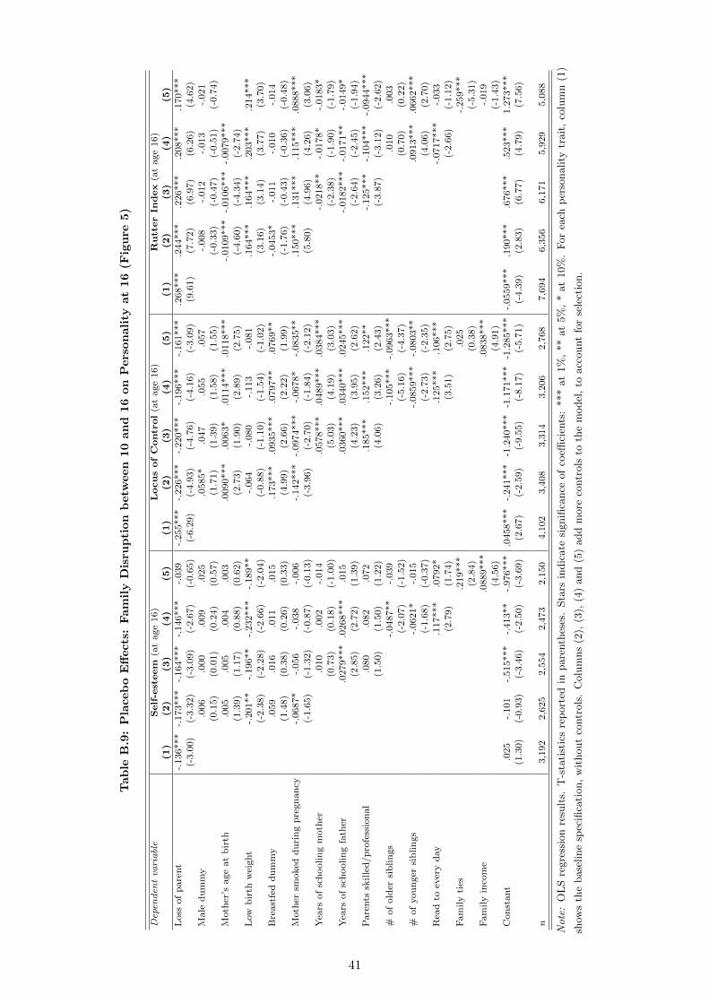
Tab
leB
.9:
Pla
ceb
oE
ffects
:Fam
ily
Dis
rup
tion
betw
een
10
an
d16
on
Pers
on
ali
tyat
16
(Fig
ure
5)
Depen
den
tva
riable
Self-esteem
(at
age
16)
LocusofControl
(at
age
16)
RutterIn
dex
(at
age
16)
(1)
(2)
(3)
(4)
(5)
(1)
(2)
(3)
(4)
(5)
(1)
(2)
(3)
(4)
(5)
Loss
of
pare
nt
-.136***
-.173***
-.164***
-.146***
-.039
-.255***
-.226***
-.220***
-.196***
-.161***
.268***
.244***
.226***
.208***
.170***
(-3.0
0)
(-3.3
2)
(-3.0
9)
(-2.6
7)
(-0.6
5)
(-6.2
9)
(-4.9
3)
(-4.7
6)
(-4.1
6)
(-3.0
9)
(9.6
1)
(7.7
2)
(6.9
7)
(6.2
6)
(4.6
2)
Male
du
mm
y.0
06
.000
.009
.025
.0585*
.047
.055
.057
-.008
-.012
-.013
-.021
(0.1
5)
(0.0
1)
(0.2
4)
(0.5
7)
(1.7
1)
(1.3
9)
(1.5
8)
(1.5
5)
(-0.3
3)
(-0.4
7)
(-0.5
1)
(-0.7
4)
Moth
er’s
age
at
bir
th.0
05
.005
.004
.003
.0090***
.0063*
.0114***
.0118***
-.0109***
-.0106***
-.0079***
(1.3
9)
(1.1
7)
(0.8
8)
(0.6
2)
(2.7
3)
(1.9
0)
(2.8
9)
(2.7
5)
(-4.6
0)
(-4.3
4)
(-2.7
4)
Low
bir
thw
eight
-.201**
-.196**
-.232***
-.189**
-.064
-.080
-.113
-.081
.164***
.164***
.203***
.214***
(-2.3
8)
(-2.2
8)
(-2.6
6)
(-2.0
4)
(-0.8
8)
(-1.1
0)
(-1.5
4)
(-1.0
2)
(3.1
6)
(3.1
4)
(3.7
7)
(3.7
0)
Bre
ast
fed
du
mm
y.0
59
.016
.011
.015
.173***
.0935***
.0797**
.0769**
-.0453*
-.011
-.010
-.014
(1.4
8)
(0.3
8)
(0.2
6)
(0.3
3)
(4.9
9)
(2.6
6)
(2.2
2)
(1.9
9)
(-1.7
6)
(-0.4
3)
(-0.3
6)
(-0.4
8)
Moth
ersm
oked
du
rin
gp
regn
an
cy-.
0687*
-.056
-.038
-.006
-.142***
-.0974***
-.0678*
-.0835**
.150***
.131***
.115***
.0888***
(-1.6
5)
(-1.3
2)
(-0.8
7)
(-0.1
3)
(-3.9
6)
(-2.7
0)
(-1.8
4)
(-2.1
2)
(5.8
0)
(4.9
6)
(4.2
6)
(3.0
6)
Yea
rsof
sch
oolin
gm
oth
er.0
10
.002
-.014
.0578***
.0489***
.0384***
-.0218**
-.0178*
-.0183*
(0.7
3)
(0.1
8)
(-1.0
0)
(5.0
3)
(4.1
9)
(3.0
3)
(-2.3
8)
(-1.9
0)
(-1.7
9)
Yea
rsof
sch
oolin
gfa
ther
.0279***
.0268***
.015
.0360***
.0340***
.0245***
-.0182***
-.0171**
-.0149*
(2.8
5)
(2.7
2)
(1.3
9)
(4.2
3)
(3.9
5)
(2.6
2)
(-2.6
4)
(-2.4
5)
(-1.9
4)
Pare
nts
skille
d/p
rofe
ssio
nal
.080
.082
.072
.185***
.152***
.122**
-.125***
-.104***
-.0944***
(1.5
0)
(1.5
0)
(1.2
2)
(4.0
6)
(3.2
6)
(2.4
3)
(-3.8
7)
(-3.1
2)
(-2.6
2)
#of
old
ersi
bli
ngs
-.0487**
-.039
-.105***
-.0963***
.010
.003
(-2.0
7)
(-1.5
2)
(-5.1
6)
(-4.3
7)
(0.7
0)
(0.2
2)
#of
you
nger
sib
lin
gs
-.0621*
-.015
-.0859***
-.0803**
.0913***
.0662***
(-1.6
8)
(-0.3
7)
(-2.7
3)
(-2.3
5)
(4.0
6)
(2.7
0)
Rea
dto
ever
yd
ay
.117***
.0792*
.125***
.106***
-.0717***
-.033
(2.7
9)
(1.7
4)
(3.5
1)
(2.7
5)
(-2.6
6)
(-1.1
2)
Fam
ily
ties
.219***
.025
-.259***
(2.8
4)
(0.3
8)
(-5.3
1)
Fam
ily
inco
me
.0889***
.0838***
-.019
(4.5
6)
(4.9
1)
(-1.4
3)
Con
stant
.025
-.101
-.515***
-.413**
-.976***
.0458***
-.241***
-1.2
40***
-1.1
71***
-1.2
85***
-.0559***
.190***
.676***
.523***
1.2
73***
(1.3
0)
(-0.9
3)
(-3.4
6)
(-2.5
0)
(-3.6
9)
(2.6
7)
(-2.5
9)
(-9.5
5)
(-8.1
7)
(-5.7
1)
(-4.3
9)
(2.8
3)
(6.7
7)
(4.7
9)
(7.5
6)
n3,1
92
2,6
25
2,5
54
2,4
73
2,1
50
4,1
02
3,4
08
3,3
14
3,2
06
2,7
68
7,6
94
6,3
56
6,1
71
5,9
29
5,0
88
Note:
OL
Sre
gre
ssio
nre
sult
s.T
-sta
tist
ics
rep
ort
edin
pare
nth
eses
.Sta
rsin
dic
ate
signifi
cance
of
coeffi
cien
ts:
***
at
1%
,**
at
5%
,*
at
10%
.F
or
each
per
sonality
trait
,co
lum
n(1
)
show
sth
ebase
line
spec
ifica
tion,
wit
hout
contr
ols
.C
olu
mns
(2),
(3),
(4)
and
(5)
add
more
contr
ols
toth
em
odel
,to
acc
ount
for
sele
ctio
n.
41

Tab
leB
.10:
Pla
ceb
oE
ffects
:Fam
ily
Dis
rup
tion
betw
een
10
an
d16
on
Pers
on
ali
tyat
10
(Fig
ure
5)
Depen
den
tva
riable
∆Self-esteem
∆LocusofControl
∆RutterIn
dex
(1)
(2)
(3)
(4)
(5)
(1)
(2)
(3)
(4)
(5)
(1)
(2)
(3)
(4)
(5)
Loss
of
pare
nt
-.138***
-.118***
-.108***
-.0913***
-.017
-.174***
-.152***
-.132***
-.118***
-.0690*
.193***
.156***
.134***
.149***
.0921***
(-4.7
5)
(-3.6
3)
(-3.2
4)
(-2.6
8)
(-0.4
7)
(-5.9
5)
(-4.6
4)
(-4.0
0)
(-3.5
4)
(-1.8
9)
(6.8
7)
(4.9
4)
(4.1
5)
(4.5
1)
(2.6
5)
Male
du
mm
y.2
18***
.214***
.212***
.231***
.042
.032
.035
.0590**
.145***
.141***
.149***
.139***
(8.5
0)
(8.2
7)
(8.0
4)
(8.2
7)
(1.6
3)
(1.2
7)
(1.3
5)
(2.1
5)
(5.8
6)
(5.6
5)
(5.8
5)
(5.2
9)
Moth
er’s
age
at
bir
th.0
076***
.0078***
.0108***
.0117***
.0099***
.0084***
.0107***
.0101***
-.0119***
-.0106***
-.0064**
-.0061**
(3.1
3)
(3.1
3)
(3.6
4)
(3.6
8)
(4.0
7)
(3.4
5)
(3.6
9)
(3.2
3)
(-5.0
3)
(-4.3
7)
(-2.2
1)
(-2.0
4)
Low
bir
thw
eight
-.112**
-.0891*
-.107*
-.085
-.224***
-.198***
-.220***
-.195***
.027
.026
.059
.033
(-2.0
9)
(-1.6
5)
(-1.9
3)
(-1.4
6)
(-4.2
0)
(-3.7
2)
(-4.0
5)
(-3.3
9)
(0.5
3)
(0.5
0)
(1.0
9)
(0.6
0)
Bre
ast
fed
du
mm
y.0
628**
.020
.008
-.011
.131***
.042
.028
.010
-.0472*
-.009
-.009
-.008
(2.3
6)
(0.7
3)
(0.2
7)
(-0.3
5)
(4.9
0)
(1.5
8)
(1.0
2)
(0.3
4)
(-1.8
4)
(-0.3
3)
(-0.3
5)
(-0.2
9)
Moth
ersm
oked
du
rin
gp
regn
an
cy-.
130***
-.0946***
-.0771***
-.0759***
-.192***
-.131***
-.110***
-.107***
.109***
.0865***
.0790***
.0526*
(-4.8
8)
(-3.4
9)
(-2.7
8)
(-2.5
8)
(-7.1
9)
(-4.9
1)
(-4.0
5)
(-3.7
1)
(4.2
1)
(3.2
9)
(2.9
5)
(1.9
0)
Yea
rsof
sch
oolin
gm
oth
er.0
365***
.0301***
.017
.0747***
.0670***
.0616***
-.0216**
-.0160*
-.012
(3.7
1)
(2.9
9)
(1.5
5)
(7.7
4)
(6.8
3)
(5.8
3)
(-2.3
3)
(-1.6
8)
(-1.2
5)
Yea
rsof
sch
oolin
gfa
ther
.0269***
.0256***
.0209***
.0472***
.0454***
.0355***
-.0283***
-.0294***
-.0262***
(3.7
0)
(3.4
7)
(2.6
3)
(6.6
1)
(6.3
0)
(4.5
5)
(-4.1
0)
(-4.2
1)
(-3.5
5)
Pare
nts
skille
d/p
rofe
ssio
nal
.050
.021
-.011
.155***
.119***
.0805**
-.0871***
-.0611*
-.046
(1.5
1)
(0.6
3)
(-0.3
1)
(4.8
0)
(3.5
8)
(2.2
7)
(-2.7
2)
(-1.8
6)
(-1.3
5)
#of
old
ersi
bli
ngs
-.0705***
-.0640***
-.0770***
-.0697***
.011
-.017
(-4.9
5)
(-4.1
5)
(-5.5
2)
(-4.6
0)
(0.7
6)
(-1.2
0)
#of
you
nger
sib
lin
gs
-.0551**
-.028
-.0896***
-.0677***
.114***
.0768***
(-2.3
6)
(-1.1
3)
(-3.9
1)
(-2.7
4)
(5.1
0)
(3.2
9)
Rea
dto
ever
yd
ay
.0727***
.0613**
.127***
.0960***
-.0782***
-.041
(2.6
1)
(2.0
5)
(4.6
7)
(3.2
8)
(-2.9
0)
(-1.4
5)
Fam
ily
ties
.152***
.150***
-.386***
(3.0
9)
(3.1
1)
(-8.3
7)
Fam
ily
inco
me
.0706***
.0676***
-.0424***
(5.2
8)
(5.1
5)
(-3.4
3)
Con
stant
.0289**
-.248***
-.914***
-.831***
-1.2
80***
.0362***
-.209***
-1.4
80***
-1.3
57***
-1.7
62***
-.0401***
.182***
.710***
.495***
1.5
59***
(2.1
7)
(-3.6
0)
(-8.6
9)
(-7.2
8)
(-7.4
8)
(2.7
2)
(-3.0
2)
(-14.3
5)
(-12.1
6)
(-1.4
6)
(-3.1
3)
(2.7
3)
(7.0
7)
(4.5
3)
(9.7
4)
n7,1
22
5,9
56
5,7
82
5,5
58
4,8
98
7,0
80
5,9
17
5,7
42
5,5
19
4,8
65
7,6
40
6,4
33
6,2
38
5,9
95
5,5
41
Note:
OL
Sre
gre
ssio
nre
sult
s.T
-sta
tist
ics
rep
ort
edin
pare
nth
eses
.Sta
rsin
dic
ate
signifi
cance
of
coeffi
cien
ts:
***
at
1%
,**
at
5%
,*
at
10%
.F
or
each
per
sonality
trait
,co
lum
n(1
)
show
sth
ebase
line
spec
ifica
tion,
wit
hout
contr
ols
.C
olu
mns
(2),
(3),
(4)
and
(5)
add
more
contr
ols
toth
em
odel
,to
acc
ount
for
sele
ctio
n.
42
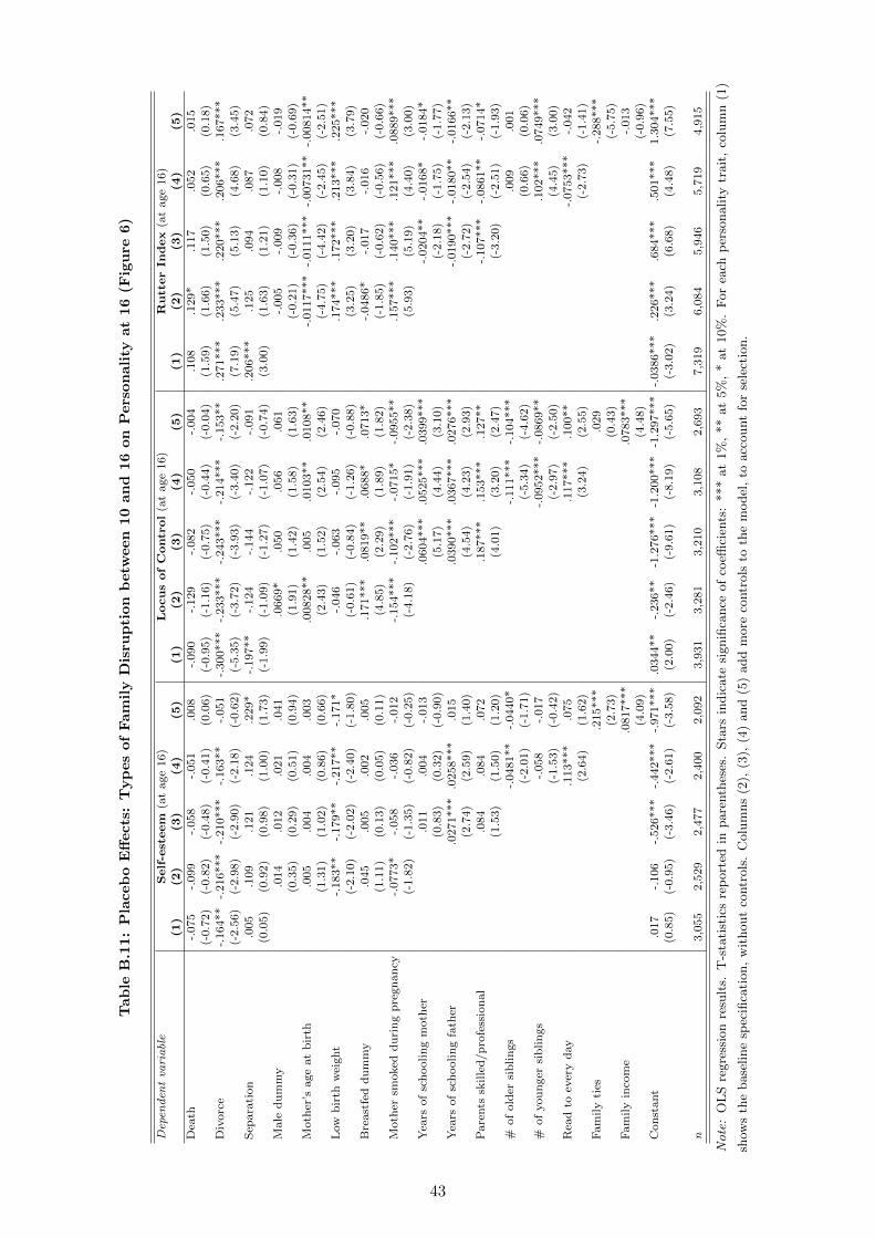
Tab
leB
.11:
Pla
ceb
oE
ffects
:T
yp
es
of
Fam
ily
Dis
rup
tion
betw
een
10
an
d16
on
Pers
on
ali
tyat
16
(Fig
ure
6)
Depen
den
tva
riable
Self-esteem
(at
age
16)
LocusofControl
(at
age
16)
RutterIn
dex
(at
age
16)
(1)
(2)
(3)
(4)
(5)
(1)
(2)
(3)
(4)
(5)
(1)
(2)
(3)
(4)
(5)
Dea
th-.
075
-.099
-.058
-.051
.008
-.090
-.129
-.082
-.050
-.004
.108
.129*
.117
.052
.015
(-0.7
2)
(-0.8
2)
(-0.4
8)
(-0.4
1)
(0.0
6)
(-0.9
5)
(-1.1
6)
(-0.7
5)
(-0.4
4)
(-0.0
4)
(1.5
9)
(1.6
6)
(1.5
0)
(0.6
5)
(0.1
8)
Div
orc
e-.
164**
-.216***
-.210***
-.163**
-.051
-.300***
-.233***
-.243***
-.214***
-.153**
.271***
.233***
.220***
.206***
.167***
(-2.5
6)
(-2.9
8)
(-2.9
0)
(-2.1
8)
(-0.6
2)
(-5.3
5)
(-3.7
2)
(-3.9
3)
(-3.4
0)
(-2.2
0)
(7.1
9)
(5.4
7)
(5.1
3)
(4.6
8)
(3.4
5)
Sep
ara
tion
.005
.109
.121
.124
.229*
-.197**
-.124
-.144
-.122
-.091
.206***
.125
.094
.087
.072
(0.0
5)
(0.9
2)
(0.9
8)
(1.0
0)
(1.7
3)
(-1.9
9)
(-1.0
9)
(-1.2
7)
(-1.0
7)
(-0.7
4)
(3.0
0)
(1.6
3)
(1.2
1)
(1.1
0)
(0.8
4)
Male
du
mm
y.0
14
.012
.021
.041
.0669*
.050
.056
.061
-.005
-.009
-.008
-.019
(0.3
5)
(0.2
9)
(0.5
1)
(0.9
4)
(1.9
1)
(1.4
2)
(1.5
8)
(1.6
3)
(-0.2
1)
(-0.3
6)
(-0.3
1)
(-0.6
9)
Moth
er’s
age
at
bir
th.0
05
.004
.004
.003
.00828**
.005
.0103**
.0108**
-.0117***
-.0111***
-.00731**
-.00814**
(1.3
1)
(1.0
2)
(0.8
6)
(0.6
6)
(2.4
3)
(1.5
2)
(2.5
4)
(2.4
6)
(-4.7
5)
(-4.4
2)
(-2.4
5)
(-2.5
1)
Low
bir
thw
eight
-.183**
-.179**
-.217**
-.171*
-.046
-.063
-.095
-.070
.174***
.172***
.213***
.225***
(-2.1
0)
(-2.0
2)
(-2.4
0)
(-1.8
0)
(-0.6
1)
(-0.8
4)
(-1.2
6)
(-0.8
8)
(3.2
5)
(3.2
0)
(3.8
4)
(3.7
9)
Bre
ast
fed
du
mm
y.0
45
.005
.002
.005
.171***
.0819**
.0688*
.0713*
-.0486*
-.017
-.016
-.020
(1.1
1)
(0.1
3)
(0.0
5)
(0.1
1)
(4.8
5)
(2.2
9)
(1.8
9)
(1.8
2)
(-1.8
5)
(-0.6
2)
(-0.5
6)
(-0.6
6)
Moth
ersm
oked
du
rin
gp
regn
an
cy-.
0773*
-.058
-.036
-.012
-.154***
-.102***
-.0715*
-.0955**
.157***
.140***
.121***
.0889***
(-1.8
2)
(-1.3
5)
(-0.8
2)
(-0.2
5)
(-4.1
8)
(-2.7
6)
(-1.9
1)
(-2.3
8)
(5.9
3)
(5.1
9)
(4.4
0)
(3.0
0)
Yea
rsof
sch
oolin
gm
oth
er.0
11
.004
-.013
.0604***
.0525***
.0399***
-.0204**
-.0168*
-.0184*
(0.8
3)
(0.3
2)
(-0.9
0)
(5.1
7)
(4.4
4)
(3.1
0)
(-2.1
8)
(-1.7
5)
(-1.7
7)
Yea
rsof
sch
oolin
gfa
ther
.0271***
.0258***
.015
.0390***
.0367***
.0276***
-.0190***
-.0180**
-.0166**
(2.7
4)
(2.5
9)
(1.4
0)
(4.5
4)
(4.2
3)
(2.9
3)
(-2.7
2)
(-2.5
4)
(-2.1
3)
Pare
nts
skille
d/p
rofe
ssio
nal
.084
.084
.072
.187***
.153***
.127**
-.107***
-.0861**
-.0714*
(1.5
3)
(1.5
0)
(1.2
0)
(4.0
1)
(3.2
0)
(2.4
7)
(-3.2
0)
(-2.5
1)
(-1.9
3)
#of
old
ersi
blin
gs
-.0481**
-.0440*
-.111***
-.104***
.009
.001
(-2.0
1)
(-1.7
1)
(-5.3
4)
(-4.6
2)
(0.6
6)
(0.0
6)
#of
you
nger
sib
lin
gs
-.058
-.017
-.0952***
-.0869**
.102***
.0749***
(-1.5
3)
(-0.4
2)
(-2.9
7)
(-2.5
0)
(4.4
5)
(3.0
0)
Rea
dto
ever
yd
ay
.113***
.075
.117***
.100**
-.0753***
-.042
(2.6
4)
(1.6
2)
(3.2
4)
(2.5
5)
(-2.7
3)
(-1.4
1)
Fam
ily
ties
.215***
.029
-.288***
(2.7
3)
(0.4
3)
(-5.7
5)
Fam
ily
inco
me
.0817***
.0783***
-.013
(4.0
9)
(4.4
8)
(-0.9
6)
Con
stant
.017
-.106
-.526***
-.442***
-.971***
.0344**
-.236**
-1.2
76***
-1.2
00***
-1.2
97***
-.0386***
.226***
.684***
.501***
1.3
04***
(0.8
5)
(-0.9
5)
(-3.4
6)
(-2.6
1)
(-3.5
8)
(2.0
0)
(-2.4
6)
(-9.6
1)
(-8.1
9)
(-5.6
5)
(-3.0
2)
(3.2
4)
(6.6
8)
(4.4
8)
(7.5
5)
n3,0
55
2,5
29
2,4
77
2,4
00
2,0
92
3,9
31
3,2
81
3,2
10
3,1
08
2,6
93
7,3
19
6,0
84
5,9
46
5,7
19
4,9
15
Note:
OL
Sre
gre
ssio
nre
sult
s.T
-sta
tist
ics
rep
ort
edin
pare
nth
eses
.Sta
rsin
dic
ate
signifi
cance
of
coeffi
cien
ts:
***
at
1%
,**
at
5%
,*
at
10%
.F
or
each
per
sonality
trait
,co
lum
n(1
)
show
sth
ebase
line
spec
ifica
tion,
wit
hout
contr
ols
.C
olu
mns
(2),
(3),
(4)
and
(5)
add
more
contr
ols
toth
em
odel
,to
acc
ount
for
sele
ctio
n.
43
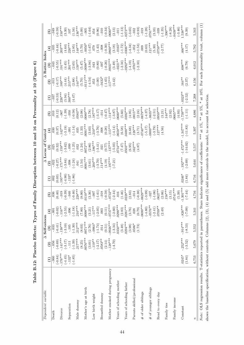
Tab
leB
.12:
Pla
ceb
oE
ffects
:T
yp
es
of
Fam
ily
Dis
rup
tion
betw
een
10
an
d16
on
Pers
on
ali
tyat
10
(Fig
ure
6)
Depen
den
tva
riable
∆Self-esteem
∆LocusofControl
∆RutterIn
dex
(1)
(2)
(3)
(4)
(5)
(1)
(2)
(3)
(4)
(5)
(1)
(2)
(3)
(4)
(5)
Dea
th-.
060
-.056
-.033
-.001
.036
.002
-.022
.025
.030
.010
-.037
-.013
-.043
-.035
-.049
(-0.8
4)
(-0.6
9)
(-0.4
1)
(-0.0
2)
(0.4
0)
(0.0
3)
(-0.2
7)
(0.3
2)
(0.3
7)
(0.1
2)
(-0.5
3)
(-0.1
7)
(-0.5
5)
(-0.4
4)
(-0.5
9)
Div
orc
e-.
176***
-.141***
-.138***
-.116**
-.019
-.195***
-.171***
-.159***
-.142***
-.067
.226***
.189***
.191***
.203***
.150***
(-4.4
5)
(-3.1
7)
(-3.1
0)
(-2.5
5)
(-0.3
9)
(-4.9
0)
(-3.8
4)
(-3.6
2)
(-3.1
9)
(-1.3
9)
(5.9
4)
(4.4
4)
(4.4
5)
(4.6
4)
(3.3
0)
Sep
ara
tion
-.132*
-.111
-.105
-.096
-.040
-.133*
-.098
-.099
-.091
-.050
.300***
.215***
.201***
.220***
.107
(-1.8
5)
(-1.3
9)
(-1.3
0)
(-1.1
8)
(-0.4
6)
(-1.8
6)
(-1.2
4)
(-1.2
5)
(-1.1
4)
(-0.5
8)
(4.4
7)
(2.8
8)
(2.6
5)
(2.8
5)
(1.3
4)
Male
du
mm
y.2
17***
.212***
.210***
.228***
.041
.032
.035
.0583**
.144***
.139***
.148***
.136***
(8.2
5)
(8.0
3)
(7.8
0)
(8.0
0)
(1.5
4)
(1.2
4)
(1.3
3)
(2.0
8)
(5.7
0)
(5.4
7)
(5.7
0)
(5.0
9)
Moth
er’s
age
at
bir
th.0
076***
.0071***
.0098***
.0110***
.0091***
.0072***
.0091***
.0089***
-.0111***
-.0098***
-.0050*
-.005
(3.0
1)
(2.7
6)
(3.2
1)
(3.3
6)
(3.6
1)
(2.8
6)
(3.0
3)
(2.7
8)
(-4.5
4)
(-3.9
4)
(-1.6
7)
(-1.6
4)
Low
bir
thw
eight
-.119**
-.0964*
-.117**
-.097
-.204***
-.186***
-.210***
-.187***
.053
.043
.079
.054
(-2.1
7)
(-1.7
4)
(-2.0
5)
(-1.6
1)
(-3.7
0)
(-3.4
1)
(-3.7
6)
(-3.1
7)
(1.0
0)
(0.8
0)
(1.4
3)
(0.9
6)
Bre
ast
fed
du
mm
y.0
583**
.014
.003
-.018
.114***
.021
.008
-.014
-.0432*
-.007
-.008
-.010
(2.1
4)
(0.5
1)
(0.1
1)
(-0.5
9)
(4.1
9)
(0.7
7)
(0.2
8)
(-0.4
7)
(-1.6
5)
(-0.2
6)
(-0.3
0)
(-0.3
4)
Moth
ersm
oked
du
rin
gp
regn
an
cy-.
128***
-.0926***
-.0737***
-.0732**
-.197***
-.137***
-.115***
-.114***
.117***
.0935***
.0869***
.0600**
(-4.7
0)
(-3.3
4)
(-2.6
0)
(-2.4
4)
(-7.2
1)
(-5.0
3)
(-4.1
4)
(-3.8
7)
(4.4
2)
(3.4
9)
(3.1
8)
(2.1
3)
Yea
rsof
sch
oolin
gm
oth
er.0
350***
.0290***
.016
.0734***
.0658***
.0600***
-.0221**
-.0165*
-.011
(3.4
8)
(2.8
3)
(1.4
6)
(7.4
7)
(6.5
8)
(5.6
0)
(-2.3
4)
(-1.7
2)
(-1.1
3)
Yea
rsof
sch
oolin
gfa
ther
.0294***
.0281***
.0228***
.0503***
.0488***
.0392***
-.0292***
-.0306***
-.0273***
(3.9
8)
(3.7
6)
(2.8
3)
(6.9
5)
(6.6
8)
(4.9
5)
(-4.1
9)
(-4.3
4)
(-3.6
5)
Pare
nts
skille
d/p
rofe
ssio
nal
.0586*
.028
-.014
.162***
.126***
.0815**
-.0767**
-.052
-.032
(1.7
3)
(0.7
9)
(-0.3
8)
(4.8
7)
(3.7
1)
(2.2
4)
(-2.3
3)
(-1.5
3)
(-0.9
3)
#of
old
ersi
bli
ngs
-.0699***
-.0629***
-.0740***
-.0679***
.009
-.019
(-4.8
0)
(-3.9
9)
(-5.1
7)
(-4.3
7)
(0.6
3)
(-1.2
8)
#of
you
nger
sib
lin
gs
-.0576**
-.027
-.0889***
-.0635**
.121***
.0791***
(-2.4
1)
(-1.0
6)
(-3.7
9)
(-2.5
1)
(5.3
0)
(3.3
3)
Rea
dto
ever
yd
ay
.0709**
.0627**
.127***
.0959***
-.0759***
-.039
(2.4
9)
(2.0
6)
(4.5
6)
(3.2
1)
(-2.7
7)
(-1.3
5)
Fam
ily
ties
.158***
.144***
-.390***
(3.1
5)
(2.9
2)
(-8.2
8)
Fam
ily
inco
me
.0741***
.0665***
-.0439***
(5.3
9)
(4.9
3)
(-3.4
6)
Con
stant
.0245*
-.252***
-.914***
-.826***
-1.3
01***
.0246*
-.192***
-1.4
72***
-1.3
47***
-1.7
39***
-.0323**
.164**
.698***
.466***
1.5
38***
(1.8
4)
(-3.5
2)
(-8.5
3)
(-7.0
9)
(-7.4
4)
(1.8
4)
(-2.6
9)
(-14.0
2)
(-11.8
3)
(-1.1
1)
(-2.5
2)
(2.3
7)
(6.7
9)
(4.1
7)
(9.3
9)
n6,7
53
5,6
79
5,5
52
5,3
41
4,7
16
6,7
16
5,6
44
5,5
17
5,3
07
4,6
86
7,2
68
6,1
56
6,0
12
5,7
82
5,3
43
Note:
OL
Sre
gre
ssio
nre
sult
s.T
-sta
tist
ics
rep
ort
edin
pare
nth
eses
.Sta
rsin
dic
ate
signifi
cance
of
coeffi
cien
ts:
***
at
1%
,**
at
5%
,*
at
10%
.F
or
each
per
sonality
trait
,co
lum
n(1
)
show
sth
ebase
line
spec
ifica
tion,
wit
hout
contr
ols
.C
olu
mns
(2),
(3),
(4)
and
(5)
add
more
contr
ols
toth
em
odel
,to
acc
ount
for
sele
ctio
n.
44
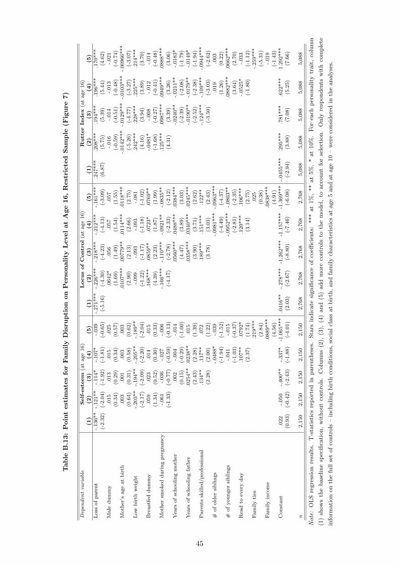
Tab
leB
.13:
Poin
test
imate
sfo
rFam
ily
Dis
rup
tion
on
Pers
on
ali
tyL
evel
at
Age
16,
Rest
ricte
dS
am
ple
(Fig
ure
7)
Depen
den
tva
riable
Self-esteem
(at
age
16)
LocusofControl
(at
age
16)
RutterIn
dex
(at
age
16)
(1)
(2)
(3)
(4)
(5)
(1)
(2)
(3)
(4)
(5)
(1)
(2)
(3)
(4)
(5)
Loss
of
pare
nt
-.136**
-.121**
-.114*
-.107*
-.039
-.271***
-.226***
-.218***
-.212***
-.161***
.247***
.208***
.194***
.196***
.170***
(-2.3
2)
(-2.0
4)
(-1.9
2)
(-1.8
1)
(-0.6
5)
(-5.1
6)
(-4.3
0)
(-4.2
3)
(-4.1
3)
(-3.0
9)
(6.8
7)
(5.7
5)
(5.3
9)
(5.4
4)
(4.6
2)
Male
du
mm
y.0
15
.013
.015
.025
.0642*
.056
.057
.057
-.016
-.014
-.013
-.021
(0.3
4)
(0.2
9)
(0.3
4)
(0.5
7)
(1.6
9)
(1.4
9)
(1.5
4)
(1.5
5)
(-0.5
9)
(-0.5
1)
(-0.4
8)
(-0.7
4)
Moth
er’s
age
at
bir
th.0
03
.001
.003
.003
.0107***
.00779**
.0114***
.0118***
-.0142***
-.0129***
-.0103***
-.00966***
(0.6
4)
(0.3
1)
(0.5
8)
(0.6
2)
(2.9
0)
(2.1
3)
(2.6
6)
(2.7
5)
(-5.2
6)
(-4.7
7)
(-3.2
7)
(-3.0
7)
Low
bir
thw
eight
-.203**
-.194**
-.205**
-.189**
-.099
-.093
-.093
-.081
.242***
.228***
.225***
.214***
(-2.1
7)
(-2.0
9)
(-2.2
0)
(-2.0
4)
(-1.2
2)
(-1.1
7)
(-1.1
8)
(-1.0
2)
(4.1
6)
(3.9
4)
(3.8
9)
(3.7
0)
Bre
ast
fed
du
mm
y.0
59
.023
.014
.015
.168***
.0859**
.0723*
.0769**
-.0481*
-.008
-.012
-.014
(1.3
4)
(0.5
2)
(0.3
0)
(0.3
3)
(4.3
9)
(2.2
3)
(1.8
7)
(1.9
9)
(-1.6
8)
(-0.2
7)
(-0.4
1)
(-0.4
8)
Moth
ersm
oked
du
rin
gp
regn
an
cy-.
061
-.036
-.027
-.006
-.166***
-.110***
-.0921**
-.0835**
.125***
.0987***
.0949***
.0888***
(-1.3
3)
(-0.7
7)
(-0.5
9)
(-0.1
3)
(-4.1
7)
(-2.7
8)
(-2.3
3)
(-2.1
2)
(4.3
1)
(3.3
9)
(3.2
6)
(3.0
6)
Yea
rsof
sch
oolin
gm
oth
er.0
02
-.004
-.014
.0560***
.0488***
.0384***
-.0240**
-.0211**
-.0183*
(0.1
5)
(-0.2
9)
(-1.0
0)
(4.4
7)
(3.8
9)
(3.0
3)
(-2.3
9)
(-2.0
8)
(-1.7
9)
Yea
rsof
sch
oolin
gfa
ther
.0254**
.0238**
.015
.0358***
.0340***
.0245***
-.0190**
-.0179**
-.0149*
(2.4
3)
(2.2
8)
(1.3
9)
(3.9
0)
(3.7
1)
(2.6
2)
(-2.5
2)
(-2.3
8)
(-1.9
4)
Pare
nts
skille
d/p
rofe
ssio
nal
.134**
.117**
.072
.189***
.151***
.122**
-.124***
-.109***
-.0944***
(2.2
8)
(2.0
0)
(1.2
2)
(3.7
8)
(3.0
3)
(2.4
3)
(-3.5
0)
(-3.0
3)
(-2.6
2)
#of
old
ersi
blin
gs
-.0488*
-.039
-.0981***
-.0963***
.019
.003
(-1.9
4)
(-1.5
2)
(-4.4
9)
(-4.3
7)
(1.2
6)
(0.2
2)
#of
you
nger
sib
lin
gs
-.041
-.015
-.0952***
-.0803**
.0882***
.0662***
(-1.0
3)
(-0.3
7)
(-2.8
1)
(-2.3
5)
(3.6
4)
(2.7
0)
Rea
dto
ever
yd
ay
.107**
.0792*
.120***
.106***
-.0525*
-.033
(2.3
7)
(1.7
4)
(3.1
4)
(2.7
5)
(-1.8
0)
(-1.1
2)
Fam
ily
ties
.219***
.025
-.259***
(2.8
4)
(0.3
8)
(-5.3
1)
Fam
ily
inco
me
.0889***
.0838***
-.019
(4.5
6)
(4.9
1)
(-1.4
3)
Con
stant
.022
-.050
-.400**
-.337*
-1.0
65***
.0416**
-.278***
-1.2
62***
-1.1
57***
-1.3
69***
-.0455***
.295***
.781***
.622***
1.2
92***
(0.9
3)
(-0.4
2)
(-2.4
3)
(-1.8
8)
(-4.0
1)
(2.0
3)
(-2.6
7)
(-8.8
0)
(-7.4
6)
(-6.0
8)
(-2.9
4)
(3.8
8)
(7.0
8)
(5.2
5)
(7.6
6)
n2,1
50
2,1
50
2,1
50
2,1
50
2,1
50
2,7
68
2,7
68
2,7
68
2,7
68
2,7
68
5,0
88
5,0
88
5,0
88
5,0
88
5,0
88
Note:
OL
Sre
gre
ssio
nre
sult
s.T
-sta
tist
ics
rep
ort
edin
pare
nth
eses
.Sta
rsin
dic
ate
signifi
cance
of
coeffi
cien
ts:
***
at
1%
,**
at
5%
,*
at
10%
.F
or
each
per
sonality
trait
,co
lum
n
(1)
show
sth
ebase
line
spec
ifica
tion,
wit
hout
contr
ols
.C
olu
mns
(2),
(3),
(4)
and
(5)
add
more
contr
ols
toth
em
odel
,to
acc
ount
for
sele
ctio
n.
Only
resp
onden
tsw
ith
com
ple
te
info
rmati
on
on
the
full
set
of
contr
ols
–in
cludin
gbir
thco
ndit
ions,
soci
al
class
at
bir
th,
and
fam
ily
chara
cter
isti
csat
age
5and
at
age
10
–w
ere
consi
der
edin
the
analy
ses.
45
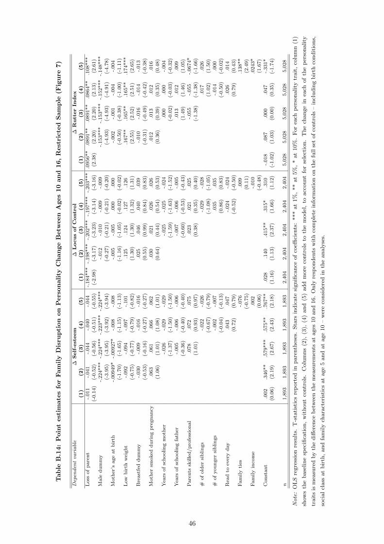
Tab
leB
.14:
Poin
test
imate
sfo
rFam
ily
Dis
rup
tion
on
Pers
on
ali
tyC
han
ge
Betw
een
Ages
10
an
d16,
Rest
ricte
dS
am
ple
(Fig
ure
7)
Depen
den
tva
riable
∆Self-esteem
∆LocusofControl
∆RutterIn
dex
(1)
(2)
(3)
(4)
(5)
(1)
(2)
(3)
(4)
(5)
(1)
(2)
(3)
(4)
(5)
Loss
of
pare
nt
-.011
-.041
-.044
-.040
-.044
-.184***
-.198***
-.202***
-.197***
-.203***
.0956**
.0891**
.0891**
.0864**
.108***
(-0.1
4)
(-0.5
2)
(-0.5
6)
(-0.5
1)
(-0.5
5)
(-2.9
8)
(-3.1
7)
(-3.2
3)
(-3.1
4)
(-3.1
6)
(2.3
8)
(2.2
0)
(2.2
0)
(2.1
3)
(2.6
1)
Male
du
mm
y-.
224***
-.224***
-.223***
-.224***
-.012
-.010
-.009
-.009
-.153***
-.153***
-.152***
-.148***
(-3.9
5)
(-3.9
5)
(-3.9
2)
(-3.9
4)
(-0.2
7)
(-0.2
1)
(-0.2
1)
(-0.2
0)
(-4.9
3)
(-4.9
3)
(-4.9
1)
(-4.7
8)
Moth
er’s
age
at
bir
th-.
00949*
-.00927*
-.008
-.008
-.005
-.005
.000
.000
-.002
-.001
-.004
-.004
(-1.7
0)
(-1.6
5)
(-1.1
5)
(-1.1
3)
(-1.1
6)
(-1.0
5)
(-0.0
2)
(-0.0
2)
(-0.5
0)
(-0.3
8)
(-1.0
0)
(-1.1
1)
Low
bir
thw
eight
-.092
-.094
-.097
-.101
.125
.124
.127
.126
.167**
.165**
.165**
.174***
(-0.7
5)
(-0.7
7)
(-0.7
9)
(-0.8
2)
(1.3
0)
(1.3
0)
(1.3
2)
(1.3
1)
(2.5
5)
(2.5
2)
(2.5
1)
(2.6
5)
Bre
ast
fed
du
mm
y-.
030
-.009
-.016
-.016
.025
.046
.040
.039
-.010
-.016
-.014
-.013
(-0.5
3)
(-0.1
6)
(-0.2
7)
(-0.2
7)
(0.5
5)
(0.9
9)
(0.8
4)
(0.8
3)
(-0.3
1)
(-0.4
9)
(-0.4
2)
(-0.3
8)
Moth
ersm
oked
du
rin
gp
regn
an
cy.0
63
.061
.066
.062
.030
.021
.026
.026
.012
.013
.012
.016
(1.0
6)
(1.0
1)
(1.0
8)
(1.0
1)
(0.6
4)
(0.4
4)
(0.5
4)
(0.5
3)
(0.3
6)
(0.3
9)
(0.3
5)
(0.4
8)
Yea
rsof
sch
oolin
gm
oth
er-.
026
-.029
-.029
-.025
-.025
-.024
.000
.000
-.004
(-1.3
7)
(-1.5
0)
(-1.5
0)
(-1.5
9)
(-1.6
3)
(-1.5
2)
(-0.0
2)
(-0.0
3)
(-0.3
2)
Yea
rsof
sch
oolin
gfa
ther
-.005
-.006
-.006
-.007
-.006
-.005
.013
.012
.009
(-0.3
6)
(-0.4
0)
(-0.4
0)
(-0.6
0)
(-0.5
3)
(-0.4
3)
(1.4
9)
(1.4
6)
(1.0
5)
Pare
nts
skille
d/p
rofe
ssio
nal
.078
.072
.075
.023
.021
.025
-.055
-.055
-.0674*
(1.0
1)
(0.9
3)
(0.9
7)
(0.3
8)
(0.3
5)
(0.4
0)
(-1.3
8)
(-1.3
8)
(-1.6
6)
#of
old
ersi
blin
gs
-.022
-.026
-.029
-.028
.017
.026
(-0.6
7)
(-0.7
9)
(-1.0
8)
(-1.0
5)
(1.0
2)
(1.5
0)
#of
you
nger
sib
lin
gs
-.002
-.007
.035
.035
-.014
.000
(-0.0
4)
(-0.1
3)
(0.8
6)
(0.8
3)
(-0.5
0)
(-0.0
2)
Rea
dto
ever
yd
ay
.043
.047
-.024
-.024
.026
.014
(0.7
2)
(0.7
9)
(-0.5
2)
(-0.5
0)
(0.7
9)
(0.4
3)
Fam
ily
ties
-.076
.009
.138**
(-0.7
5)
(0.1
1)
(2.4
9)
Fam
ily
inco
me
.002
-.010
.0243*
(0.0
6)
(-0.4
8)
(1.6
7)
Con
stant
.002
.346**
.579***
.575**
.767**
.028
.140
.415**
.315*
.310
-.018
.087
.000
.047
-.331*
(0.0
6)
(2.1
9)
(2.6
7)
(2.4
3)
(2.1
8)
(1.1
6)
(1.1
3)
(2.3
7)
(1.6
6)
(1.1
2)
(-1.0
2)
(1.0
3)
(0.0
0)
(0.3
5)
(-1.7
4)
n1,8
93
1,8
93
1,8
93
1,8
93
1,8
93
2,4
04
2,4
04
2,4
04
2,4
04
2,4
04
5,0
28
5,0
28
5,0
28
5,0
28
5,0
28
Note:
OL
Sre
gre
ssio
nre
sult
s.T
-sta
tist
ics
rep
ort
edin
pare
nth
eses
.Sta
rsin
dic
ate
signifi
cance
of
coeffi
cien
ts:
***
at
1%
,**
at
5%
,*
at
10%
.F
or
each
per
sonality
trait
,co
lum
n(1
)
show
sth
ebase
line
spec
ifica
tion,
wit
hout
contr
ols
.C
olu
mns
(2),
(3),
(4)
and
(5)
add
more
contr
ols
toth
em
odel
,to
acc
ount
for
sele
ctio
n.
The
change
inea
chof
the
per
sonality
trait
sis
mea
sure
dby
the
diff
eren
ceb
etw
een
the
mea
sure
men
tsat
ages
10
and
16.
Only
resp
onden
tsw
ith
com
ple
tein
form
ati
on
on
the
full
set
of
contr
ols
–in
cludin
gbir
thco
ndit
ions,
soci
al
class
at
bir
th,
and
fam
ily
chara
cter
isti
csat
age
5and
at
age
10
–w
ere
consi
der
edin
the
analy
ses.
46