NBER WORKING PAPER SERIES

THE EFFECT OF EDUCATION ON MORTALITY AND HEALTH:EVIDENCE FROM A SCHOOLING EXPANSION IN ROMANIA

Ofer MalamudAndreea Mitrut

Cristian Pop-Eleches

Working Paper 24341http://www.nber.org/papers/w24341

NATIONAL BUREAU OF ECONOMIC RESEARCH1050 Massachusetts Avenue

Cambridge, MA 02138February 2018

We would especially like to thank Andreea Balan-Cohen for her work on the schooling reform in Romania for a different project that is still in progress. Andreea Mitrut gratefully acknowledge support from Jan Wallanders and Tom Hedelius Fond. We have benefited from comments by participants at the ERMAS 2017 and the CHERP conference at the Federal Reserve Bank of Chicago. All errors are our own. The views expressed herein are those of the authors and do not necessarily reflect the views of the National Bureau of Economic Research.

NBER working papers are circulated for discussion and comment purposes. They have not been peer-reviewed or been subject to the review by the NBER Board of Directors that accompanies official NBER publications.

© 2018 by Ofer Malamud, Andreea Mitrut, and Cristian Pop-Eleches. All rights reserved. Short sections of text, not to exceed two paragraphs, may be quoted without explicit permission provided that full credit, including © notice, is given to the source.

The Effect of Education on Mortality and Health: Evidence from a Schooling Expansion inRomaniaOfer Malamud, Andreea Mitrut, and Cristian Pop-ElechesNBER Working Paper No. 24341February 2018JEL No. I1,I12,I15,I25,I26

ABSTRACT

This paper examines a schooling expansion in Romania which increased educational attainment for successive cohorts born between 1945 and 1950. We use a regression discontinuity design at the day level based on school entry cutoff dates to estimate impacts on mortality with 1994-2016 Vital Statistics data and self-reported health with 2011 Census data. We find that the schooling reform led to significant increases in years of schooling and changes in labor market outcomes but did not affect mortality or self-reported health. These estimates provide new evidence for the causal relationship between education and mortality outside of high-income countries and at lower margins of educational attainment.

Ofer MalamudSchool of Education and Social Policy Northwestern UniversityAnnenberg Hall2120 Campus DriveEvanston, IL 60208and NBERofer.malamud@northwestern.edu

Andreea MitrutUniversity of GothenburgDepartment of EconomicsBox 640405 30 Göteborg, Sweden andreea.mitrut@economics.gu.se

Cristian Pop-ElechesThe School of International and Public AffairsColumbia University1401A International Affairs Building, MC 3308420 West 118th StreetNew York, NY 10027and NBERcp2124@columbia.edu

2

1. Introduction

There is substantial evidence showing that more educated people have better

health and longer life expectancies. However, whether this correlation reflects a causal

relationship remains an open question. A number of recent papers have used changes in

compulsory schooling requirements to identify the causal impact of schooling on health

and mortality in the United States (Lleras-Muney, 2005; Mazumder, 2008), the United

Kingdom (Oreopoulos, 2006; Clark and Royer, 2013), Denmark (Arendt, 2008), France

(Albouy and Lequien, 2009), the Netherlands (van Kippersluis, et al., 2011), and Sweden

(Meghir, et al., forthcoming). While this empirical approach can be compelling, the

findings have been mixed and sometimes contradictory, even when based on the same

educational expansions. Moreover, all of these studies are focused on the United States

or Western Europe where compulsory schooling laws usually affect students enrolled in

secondary school. As a result, we know relatively little about the causal effect of

education on health and mortality in developing or middle-income countries, and at

lower margins of educational attainment.

This paper examines the impact of a schooling expansion in Romania during the

late 1950s and early 1960s, which sought to provide all students with at least 7 years of

compulsory education. We show that successive cohorts of individuals, born between

1945 and 1950, who were affected by this schooling expansion, experienced rising

educational attainment. Then we use a regression discontinuity design at the day level

to compare individuals born just before the school entry cutoff of January 1 to those

born just after, who were almost identical in age but began school later and therefore

had greater opportunities to extend their education. Since students born immediately

before and after January 1 were also the oldest and youngest in their respective classes,

3

we also draw on cohorts born after the schooling expansion had concluded to separate

the effect of increased education from that of relative age and starting school younger.1

We demonstrate that the schooling expansion led to significant increases in

years of schooling for the affected cohorts born between 1945 and 1950. This increase

in educational attainment was accompanied by significant increases in labor force

participation and decreases in fertility for women. Nevertheless, using detailed

information on deaths from Vital Statistics data between 1994 and 2016, we do not find

evidence that the schooling expansion reduced the mortality of affected cohorts up to

the age of 71. Nor are there reductions in mortality from more specific causes of death.

In addition, there are no significant effects for measures of self-reported health using

data from the 2011 Romanian Census.

Our findings indicate that more education does not help individuals avoid or

postpone deaths during middle and old age. This is consistent with the null results in

the most recent papers by Clark and Royer (2013) and Meghir et al. (forthcoming) for

the United Kingdom and Sweden. However, to the best of our knowledge, this is the first

paper to provide compelling estimates for the causal relationship between education

and mortality outside of high-income countries and at lower margins of educational

attainment. We do not interpret these estimates as an argument against further

educational expansions in the developing world. But they do suggest the need to be

more circumspect about the potential for such expansions to improve health and

increase life expectancy, at least at lower margins of educational attainment.

1 See Cascio and Schanzenbach (2016) for evidence on the impacts of relative age in Tennessee and Black, Devereux, and Salvanes (2011) for evidence on the effect of starting school younger in Norway.

4

The paper is organized as follows. Section 2 reviews the related literature.

Section 3 provides a background of the Romanian educational system and the

educational expansion. Section 4 describes the data and the empirical strategy. Section

5 presents the results, alternative explanations and potential mechanisms, while Section

6 concludes.

2. Related Literature

This section reviews some of the previous literature estimating the causal impact

of education on health and mortality. We begin with a more detailed discussion of the

papers that take advantage of changes in compulsory schooling requirements. Then we

describe some of the alternative empirical approaches used for identifying the causal

effect of education at higher margins of educational attainment. For more detailed

reviews of these and other studies, see Mazumder (2012) and Galama et al. (2018).

For the United States, Lleras-Muney (2005) uses Census data to examine the

impact of changes in compulsory schooling laws between 1915 and 1939 that affected

students over 14 years of age. Her instrumental variables (IV) estimates indicate that an

additional year of schooling leads to significant declines in the probability of dying in

the next 10 years. In a follow-up study, Mazumder (2008) notes that these results are

not robust to including state-specific trends but presents evidence from the Survey of

Income and Program Participation (SIPP) showing positive impacts of education on self-

reported health status. Finally, Black et al. (2016) argue that virtually all of the variation

in mortality rates is captured by cohort effects and state effects, making it difficult to

5

reliably estimate the effects of changing educational attainment due to state-level

changes in compulsory schooling.2

For the United Kingdom, Clark and Royer (2013) use changes to British

compulsory schooling laws in 1947 and 1972 that increased the minimum school

leaving age from 14 to 15 and then from 15 to 16. Their regression discontinuity (RD)

design does not provide strong evidence for an impact of education on mortality or

other health outcomes. Davies et al. (2016) re-examine the 1972 change in compulsory

schooling using UK Biobank data and find a statistically significant decline in mortality

but their results are somewhat sensitive to functional form.

Other studies are focused on European countries: For Sweden, Meghir et al.

(forthcoming) do not find improvements in mortality and other health measures for

affected cohorts following an educational reform in Sweden that raised the number of

years of compulsory schooling from 7/8 to 9, eliminated early selection based on

academic ability, and introduced a national curriculum. Arendt (2005) and Albouy and

Lequien (2009) also find no statistically significant impact of compulsory school

reforms on health outcomes in Denmark and France, respectively. Yet van Kippersluis et

al. (2011) do find that increasing compulsory school beyond grade 6 in the Netherlands

leads to significant reduction in mortality in old age.

Finally, a different set of studies use draft avoidance behavior in the United

States during the Vietnam War to estimate the impact of college education on mortality

and health outcomes. Buckles et al. (2016) show that the increased college going among

men in cohorts associated with greater draft avoidance also leads to lower mortality in

2 In a paper that considers the effect of school quality on health, Aaronson et al. (2017) find that childhood exposure to Rosenwald schools in the Jim Crow south increased life expectancy, after accounting for the negative effects of migration.

6

subsequent years. Grimard and Parent (2007) and de Walque (2007) use a similar

identification strategy to estimate impacts on smoking behavior and find evidence

suggesting that more education reduces the take-up of smoking and current smoking.

However, the estimates in these papers are based on changes at the margin of college

education, which may differ from changes due to compulsory schooling laws.

In our own review of the literature, and in those by Mazumder (2012) and

Galama et al. (2018), we have not found any papers that provide compelling causal

estimates for the impact of education on health or mortality in low and middle-income

countries.

3. Background on Education in Romania

During the post-war period, the structure and the organization of education in

Romania was largely based on the model in the Soviet Union as codified by Decree No.

175 of 1948 (Braham, 1972).3 There were several different types of schools. First, there

were 4-year primary schools that offered grades 1 through 4 and were often located in

rural areas. Second, there were 7-year general schools, called gymnasiums, which

offered grades 1 through 7 (and later expanded to grade 8), with the first four years

covering similar material as in the 4- year primary schools. Third, there were 11-year

schools, which offered grades 1 through 11 in one school that provided both primary

and secondary education.

After a successful campaign to provide basic literacy education targeted towards

all ages in the late 1940s and early 1950s, the government focused its attention on

increasing enrollment beyond the first four grades. According to Giurescu et al. (1971, p.

3 This section relies heavily on information provided in Barham (1963, 1972).

7

351), the five year plan of 1955-1960 specified that the extension of compulsory

schooling to 7 years was to be given special attention by the party and government.

Thus, the directives of the Communist Party’s Second Congress of 1955 which outlined

the second five year plan, envisioned a “situation under which, by 1960-1961, the fifth

grade would enroll 90 percent of the 4-year school graduates, and under which,

according to the Third Five Year plan, the 7-year school would be universal and

compulsory. At first only the first four grades were made compulsory, but villages and

rural communities having 7-year schools were required by virtue of Decision No.

1035/1958 to make the 7 year schooling period universal beginning with the 1958-

1959 academic year” (Braham, 1963).

Nevertheless, this process was not immediate and was constrained by a lack of

enough schools offering 7 years of compulsory schooling: “Since this governmental

action applied only to places where 7-year schools already existed, it appears that the

extension of free compulsory education is to a large extent only nominal. Furthermore,

with rural communities retaining the 4-year compulsory level, the lack of detailed

planning to elevate their schools to the 7-year compulsory level has left an irregular

pattern of schooling in the provinces” (Braham, 1963). Filipescu and Oprea (1972) also

confirm the gradual process of expanding education at the gymnasium level. They

explain that the expansion of 7-year compulsory education began in 1956 within towns

and larger villages that already had schools beyond the 4th grade, and that it gradually

expanded until it was close to universal by 1961-1962.

We can document some of these changes using aggregate data on enrollment

from the Annual Statistics of the Socialist Republic of Romania. Figure 1 shows the large

increase in the number of students graduating from gymnasium between 1955 and

1965. During this period, graduation from gymnasiums increased sharply from 116,698

8

in 1959 to 329,739 in 1963 and stayed at similar levels through the late 1960s and early

1970s.

Further evidence for these dramatic changes can be observed at the cohort level.

By law, students entered grade 1 in September of the year following the calendar year in

which they reached 6 years of age. Thus, the cohort born in 1945 was 6 years of age in

1951, entered first grade in the fall of 1952, entered fifth grade in the fall of 1956 and

would have graduated with 7 years of schooling in the spring of 1959. This cohort

should be the first cohort that could have been affected by the policy reform. Similarly,

the cohort born in 1947 was the first cohort to have potentially benefited from the 1958

Government Decision that made 7-year of schooling compulsory. Finally, the cohort that

entered fifth grade in 1961-1962, which according to Filipescu and Oprea (1972) is the

first cohort to have achieved universal 7 year compulsory education, was born in 1950.

Figure 2 shows the highest educational attainment by year of birth for cohorts of

individuals in the Romanian Census of 1992. There is a sharp decline in the proportion

of individuals with primary education between cohorts born in 1944 and 1950. At the

same time, we observe a sharp increase in the proportion of individuals who complete

secondary education (which includes graduates of gymnasiums). Note that cohorts born

between 1935 and 1944 also experienced large increases in educational attainment.

This is mainly driven by the early literacy and education campaigns introduced after the

Communist government came to power.

In Figure 3 we plot the “residual” percent of individuals born between 1943 and

1955 who completed primary education by their month of birth, after accounting for

calendar month of birth effects. A number of interesting patterns emerge from this

graph. First, and consistent with the results in Figure 2, we observe the large decrease

in the proportion of students who have only primary education for those born between

9

1945 and 1950. Secondly, and more importantly for our empirical strategy, the

decreases in percent of students with only primary education occur discontinuously,

with disproportionately large decreases for those born after January 1st in this period.

The discontinuities are especially visible for those born around January 1st of 1945,

1947, 1948 and 1949 and to a smaller extent for those born around January 1st of 1946

and 1950. At the same time, no similar discontinuities are visible for the control cohorts

born between 1950 and 1953. The patterns in Figure 3 suggest that we can use detailed

information on date of birth to estimate the impact of these educational expansions

using a regression discontinuity design.

To summarize, the evidence on graduation rates from gymnasiums in the

aggregate data coincides with the cohort analysis of educational attainment in the 1992

Census; and both are broadly consistent with the historical record of educational

reforms in Romania. Together, they indicate that education levels past the first 4 years

of primary schooling started to expand in the 1956-1957 school-year and by 1961-

1962, enrollment in the 5th grade was essentially universal. In other words, the

expansion affected cohorts born starting in 1945 and universal gymnasium education

was essentially completed for cohorts born in or after 1950.

4. Data and Empirical Strategy

4.1 Data

Our main sample consists of individuals born in Romania between 1944 and 1952.

Those born from 1945-1949 were enrolled in the affected grades during the period of

schooling expansion while those born from 1950-1952 were enrolled after the

10

expansions had already been completed.4 We put together information on these cohorts

from several different datasets.

We use the 1992 Romanian Census, when individuals were 40 to 48 years of age,

to estimate the impact of the schooling reform on educational attainment; certain labor

market outcomes, and conduct specification checks of our empirical strategy.5 Two

features make this dataset especially useful for our analysis: First, with 35,000 to

45,000 observations in each yearly birth cohort, we have sufficient power to employ a

regression discontinuity design. Second, there is detailed information about the day,

month, and year of birth so we can identify the discontinuity induced by the policy

within a narrow window.

The 1992 Census provides detailed information about the highest level of

educational attainment for each respondent according to the following categories: none,

primary, gymnasium, secondary education, post-secondary, and university education.

For simplicity, we impute years of schooling by assigning the number of years

associated with each level of education.6 This serves as our main summary measure of

education when estimating the impact of the schooling expansion. The Census also has

information on socio-economic characteristics of our respondents, such as gender,

ethnicity, and region of birth. We use these variables to validate our research design.

Finally, it contains information on labor force participation and occupational status (for

4 We use the three subsequent cohorts born immediately after the end of the schooling expansion as our preferred comparison group both because they are most similar in age to the cohorts affected by the schooling expansion and offer sufficiently large samples. However, our results are essentially unchanged when we use four, five, or six subsequent cohorts as our comparison group. 5 This is a 15% random sample taken from the full Romanian Census by the Population Activities Unit (PAU) of the United Nations Economic Commission for Europe (UNECE). 6 We also use data collected by the Romanian National Statistics Institute in 1995 and 1996 with reports of actual years of schooling (rather than educational attainment) in order to validate our imputed measure of years of schooling. These data come from surveys based on the 1994 World Bank’s Living Standards Measurement Studies (LSMS) for Romania.

11

those employed) as well as the fertility of women, which serve as useful auxiliary

outcomes.

Panel A of Table 1 presents summary statistics for the individuals in cohorts

born between 1944 and 1952. The average age at the time of the 1992 census is 42.2

years and the fraction of female respondents is almost exactly half. Almost 90 percent of

the sample is ethnic Romanian, with about 7 percent ethnic Hungarians, and about 1.5

percent are Roma. The average imputed years of schooling in our sample is 9.58 years.

We use the 1994-2016 Vital Statistics Mortality files (VSM) to estimate the impact

of the schooling expansion on mortality. These data cover the universe of deceased

persons in Romania with detailed information about their socio-economic

characteristics, including the day of birth/death and the main cause of death. Thus, we

can observe mortality for the cohorts used in our analysis between the ages of 42 and 71

by day and year of birth.7 We compute mortality for the cohorts born between 1944 and

1952 by dividing the total deaths of these cohorts during the period 1994-2016 to the

population at risk defined here as the 1944-1952 cohorts (alive) at the 1992 census.8

Our calculation of the mortality rate may differ from the true mortality because of

migration in and out of Romania. The number of immigrants (for the cohorts we study

here) is close to zero and should not affect our results. Moreover, the VSM files include all

people deceased abroad as long as they still have a Romanian residence and/or

citizenship. Therefore, our mortality files should account for the majority of the

Romanian migrants abroad who are temporary emigrants and do not change their

7 Lleras-Muney (2005) and Clark and Royer (2013) suggest that the largest effects of education on mortality occur before the age of 64. Life expectancy in Romania was 69.5 years in 1994, 74.2 in 2011, and 75.5 years in 2016. 8 We use sample weights to calculate the total population because we only have a 15% census sample.

12

permanent residence. 9 But we also directly examine the potential for bias due to

migration by checking whether schooling expansion affects the probably of migration.

The VSM file provides detailed information on the main cause of death so we are

able to look separately at deaths associated with circulatory diseases and cancer. These

are the two most important causes of death in Romania, accounting for 44.6% and 26.5%

respectively of all deaths. Similar to Meghir et al. (2017) we also reclassify diseases

according to the epidemiological literature as preventable and treatable; preventable

causes of death may reflect health behaviors while the treatable causes of death may be

related to access to healthcare.10

Panel B of Table 1 shows the overall mortality rate and the mortality rate by

category for our main sample. Approximately 26 percent of our sample died between

1994-2016. The largest category of deaths was due to circulatory diseases which account

for 10.5 percentage points, followed by cancer and preventable deaths, at 47.7 and 5.9

percentage points respectively. Treatable diseases only accounted for 3.9 percentage

points.

Finally, we use the 2011 Romanian Census to compute a self-reported measure of

health, which provides the impact of the schooling expansion on individuals who

survived until 2011. All respondents are asked whether they have any health related

problems that may affect their daily life at work, school, at home, etc. Approximately 7.6

percent of people in our cohorts of interest reported having such problems. Those who

answered affirmatively were given a set of six follow-up questions – whether they were

(i) visually, (ii) hearing, or (iii) movement impaired, (iv) whether they had any memory

9 According to Statistics Romania these emigrants are the vast majority (over the 95%) of emigrants. 10 We use the ICD 10 codes for defining cancer, circulatory diseases and treatable and preventable causes of death. See the Notes at the end of the tables for more information.

13

or concentration problems, (v) self-care or (vi) difficulties in communication with their

peers.

4.2 Empirical Strategy

As described earlier, the schooling expansions in Romania occurred over a five

year period from 1956 to 1961 and affected born between 1945 and 1950. Since the

government rapidly expanded access to schooling during this period, a child born just

after January 1 would have benefited from the additional schools slots created by the

government over the course of a year, as compared to a child born just before January 1

who would have been part of an earlier cohort. Indeed, the discontinuities in the

fraction of individuals whose highest level of education was primary school were clearly

visible in Figure 3 for the years 1945, 1947, 1948 and 1949. In this section, we estimate

these discontinuities more formally using a regression discontinuity (RD) design.

We estimate the differences across successive cohorts during the period of

educational expansion (i.e. in the “treatment years” of 1945-1950) using the following

equation:

𝑦𝑦𝑖𝑖 = 𝛽𝛽′𝑋𝑋𝑖𝑖 + 𝛼𝛼𝐴𝐴𝐴𝐴𝐴𝐴𝐴𝐴𝐴𝐴𝑖𝑖 + 𝑓𝑓(𝑑𝑑𝑑𝑑𝑦𝑦𝑖𝑖) + 𝜀𝜀𝑖𝑖 (1)

where 𝑦𝑦𝑖𝑖 is an outcome such as education or mortality for individual 𝑖𝑖, 𝑋𝑋𝑖𝑖 is a set of

control variables, 𝐴𝐴𝐴𝐴𝐴𝐴𝐴𝐴𝐴𝐴𝑖𝑖 is an indicator for individuals born just after the school entry

cutoff of January 1, and 𝑓𝑓(𝑑𝑑𝑑𝑑𝑦𝑦𝑖𝑖) is a parametric or non-parametric function of the day of

birth which serves as our running variable. For simplicity, our preferred specifications

do not include any control variables except for a constant, although including them does

not affect our results. The coefficient on 𝛼𝛼 is an estimate for the effect of being born just

after the school entry cutoff on the relevant outcome. When the outcome is a measure of

14

education, such as years of schooling, it represents a “first stage” estimate; when the

outcome is a measure of health, such as mortality, it represents the “reduced-form”

estimate.

If we assume that the exclusion restriction holds (i.e. that being born after the

school entry cutoff affects mortality only through years of schooling), the ratio of the

reduced-form and first stage coefficients represents an estimate for the impact of

education on mortality. However, the exclusion restriction may not hold since those

individuals born just after the school entry cutoff are generally the oldest children in

their class; that is, if relative age has an independent effect on health or mortality.

In order to account for any independent effect of relative age, we also compare

individuals who were born just before and after the school entry cutoff in a period

without educational expansion (i.e. in the “control years” of 1950-1953). We do this by

estimating a regression equation similar to equation (1) above using this set of control

years. But we also estimate the following models that directly compare the impact of

being born just after the school entry cutoff in treatment years to control years:

𝑦𝑦𝑖𝑖 = 𝛽𝛽′𝑋𝑋𝑖𝑖 + 𝛼𝛼𝐴𝐴𝐴𝐴𝐴𝐴𝐴𝐴𝐴𝐴𝑖𝑖 + 𝛾𝛾𝐴𝐴𝐴𝐴𝐴𝐴𝐴𝐴𝐴𝐴𝑖𝑖 + 𝛿𝛿𝐴𝐴𝐴𝐴𝐴𝐴𝐴𝐴𝐴𝐴𝑖𝑖 ∗ 𝐴𝐴𝐴𝐴𝐴𝐴𝐴𝐴𝐴𝐴𝑖𝑖 + 𝑓𝑓(𝑑𝑑𝑑𝑑𝑦𝑦𝑖𝑖) + 𝜀𝜀𝑖𝑖 (2)

where 𝐴𝐴𝐴𝐴𝐴𝐴𝐴𝐴𝐴𝐴𝑖𝑖 is an indicator for individuals born during years of educational

expansion 1945-1950, and the other variables are defined as before (with some abuse

of notation). In this specification, the coefficient on the interaction term, 𝛿𝛿, yields the

impact of being born just after the school entry cutoff during treatment years over and

above the effect in control years that did not experience educational expansions.

A key consideration when implementing a regression discontinuity design is the

functional form of the forcing variable, 𝑓𝑓(𝑑𝑑𝑑𝑑𝑦𝑦𝑖𝑖). We present estimates using a local

linear regression as suggested by Hahn, Todd, and van der Klaauw (2001). The choice of

15

the window is somewhat arbitrary as we need to strike a balance between the

advantages of having more precise estimates with larger windows and mitigating the

possibility of confounding time effects with more narrow windows. Therefore, for our

main tables we present specifications using a 180, 120, 90, 60 and 30 day intervals, as

well as the Imbens-Kalyanarman (IK) optimal bandwidth (Imbens and Kalyanarman,

2012). We also confirm that our results are robust to using parametric specifications

that include higher order polynomials such as linear, quadratic and cubic trends in day

of birth (results available by request). All regressions cluster on day of birth in order to

avoid the problems associated with specification error in the case of discrete covariates

(Lee and Card, 2008).

A common specification check for the regression discontinuity design is to verify

that the density of observations is continuous around the cutoff (McCrary, 2008). When

we examine the density, we find substantial heaping on January 1 and on some of the

days immediately preceding it.11 We believe that this heaping is due to delays in the

reporting of births that occurred during the holiday period between Christmas and New

Year’s Day when government offices were closed.12

Insofar as this type of heaping is similar for our “treatment” and “control” years,

we can account for this issue in the regression that uses both sets of years. However, we

also attempt to deal with this issue using a “donut-RD” design as suggested by Barreca,

Lindo, Waddel (2016). In particular, we present all of our results when dropping

individuals born within 7 days of January 1 in order to be symmetric around the cutoff.

Results are qualitatively similar when we exclude individuals born more than one week

11 These density tests are shown in Appendix Table 1 and Appendix Figure 1. They are structured in a similar fashion to the main tables as described in the results section. 12 Indeed, it appears the spike in observations occurs on January 2 in years when January 1 is a Sunday.

16

before or after January 1 or when we exclude individuals born only one or several days

before January 1 (available by request).13

5. Results

5.1 Effects on educational attainment

We begin by estimating the impact of the schooling expansion on years of completed

schooling based on the level of education recorded in the 1992 Census. These “first

stage” results are shown in Table 2 which has three panels: Panel A presents estimates

for 𝛼𝛼 from equation (1) using the treatment years, 1945-1950; Panel B presents

estimates for 𝛼𝛼 from equation (1) using the control years, 1950-1953; Panel C presents

estimates for 𝛼𝛼 and 𝛿𝛿 from our preferred specification (2) which includes both

treatment and control years. Columns (1) to (6) in each panel show estimates for

alternative bandwidths. These include 180, 120, 90, 60 and 30 days of the January 1

cutoff, as well as the optimal bandwidth proposed in Imbens and Kalyanaraman (2012).

Columns (7) to (12) show analogous specifications that exclude observations within 7

days of the January 1 cutoff (i.e. 7 day donut-RD regressions).

Panel A of Table 2 indicates that each successive cohort during the school

expansion period 1945-1950 received an additional 1/5 to 3/5 years of schooling; the

point estimates for the impact of being born just after vs. just before the January 1 cutoff

in the treatment years range from 0.21 to 0.67 years of schooling using our different

bandwidths. In contrast, the estimates in Panel B showing the impact of being born just

after vs. just before January 1 in the control years of 1950-1953 are small and

13 We also verify that our available covariates vary smoothly around the discontinuity in Appendix Tables 2 and 3. With a few exceptions, the coefficients are mostly small and insignificant.

17

statistically insignificant in all specifications. Panel C shows estimates from the

specification that combines both treatment and control years. In these specifications,

the impact of the school expansion is captured by 𝐴𝐴𝐴𝐴𝐴𝐴𝐴𝐴𝐴𝐴𝑖𝑖 ∗ 𝐴𝐴𝐴𝐴𝐴𝐴𝐴𝐴𝐴𝐴𝑖𝑖 and shows impacts

of 0.23 to 0.59 years of schooling, all highly significant. The results using the donut

specifications are about 30% smaller in magnitude but still statistically significant in all

specifications.14 The range of these estimate is not altogether surprising given the large

number of different specifications that we consider. However, we take our preferred

specification to be the IK bandwidth for the full sample, implying a first stage effect of

approximately a 1/2 year of schooling.

We also present our “first stage” results graphically in Figure 4. Panels A, C and E

plot average years of schooling by day of birth for individuals born six months before

and after January 1st of each year; panels B, D and F plot the same data by week of birth,

which often makes it easier to discern the patterns. The graphs are normalized so that

day 1 corresponds to January 1 and week 1 corresponds to the week of January 1 to

January 7. The fitted lines are based on smoothed local linear regressions using the IK

bandwidth.

Panels A and B show a clear discontinuity after January 1 for the treatment years

of 1945-1950. This visual evidence confirms that individuals born merely a couple of

days apart received a substantially different amount of schooling as a result of the

school expansion. In contrast, panels C and D of Figure 4 reveal no change in average

educational attainment before and after January 1st in the control cohort. Nevertheless,

each of the first four panels in Figure 4 show some time trends, consistent with the

14 Appendix Table 4 uses the 1994-1996 LSMS datasets to estimate the impact of the schooling expansion on reported years of schooling rather than an imputed measure based on completed educational levels. The results are somewhat less precise but generally similar to those in Table 4.

18

presence of seasonality in the timing of births. Such time effects are not visible in Panels

E and F of Figure 4, which use both treatment and control years to estimate a version of

equation (2) that differences out the impacts in the control years from those in the

treatment years.

5.2 Effects on mortality and self-reported health

In this section we analyze whether, in addition to affecting education, the school

expansion policy had an impact on mortality and health. We begin by using the Vital

Statistics data from 1994 to 2016 to examine mortality. Table 3, which has the same

structure as the previous tables, reveals no evidence of a statistically significant effect of

being born just after vs. just before the January 1 cutoff on mortality in the treatment

years of 1945-1950 (in Panel A) or in the control years of 1950-1953 (in Panel B),

except for the smallest bandwidths. Furthermore, all of the significant effects disappear

once we consider the donut regression that excludes individuals born 7 days before and

after January 1.

We see a couple of marginally significant effects on 𝐴𝐴𝐴𝐴𝐴𝐴𝐴𝐴𝐴𝐴𝑖𝑖 ∗ 𝐴𝐴𝐴𝐴𝐴𝐴𝐴𝐴𝐴𝐴𝑖𝑖 in Panel C

that includes both treatment and control years, although these have positive signs. Still,

with 10 out of the 12 point estimates from our preferred specification in Panel C not

showing any statistically significant effect, we conclude that there is no evidence for an

impact of the schooling expansion on mortality. Given the standard errors for our full

sample, we can rule out with 95% confidence that the schooling expansions reduced

mortality by more than 0.8 percentage points between 1994-2016 when the average

mortality rate was 26 percent.

A graphical analysis of the mortality results is presented in Figure 5, structured

similarly to the preceding figures. The patterns in Panels A-F provide a visual

19

interpretation of the regression estimates from Table 3. We do not see evidence for

large discontinuities in the mortality rate between 1994 and 2016 and, if anything, they

point against the finding that education reduces mortality.

We also consider the effect of the schooling expansion on specific causes of

death. We first focus on mortality from the two most common causes of death in

Romania: cancer and circulatory diseases. The regression estimates for these causes of

death are shown in Tables 4 and 5 respectively, while the figures are shown in

Appendix Figure 2 and 3 respectively. We also classify certain causes of death as

preventable or treatable, similar to Meghir et al. (2017). The regression estimates for

these causes of death are shown in Appendix Table 5 and 6 respectively. In none of the

tables do we observe evidence for a consistent effect of the schooling expansion on

mortality. Similarly, none of the corresponding graphs show visible discontinuities

around the regression discontinuity cutoffs. Thus, we do not find any more evidence for

the impact of the schooling expansion on specific causes of death than on the mortality

rate as a whole.

In addition to the impact of the schooling expansion on mortality, we also

examine its effect on self-reported health using the 2011 Romanian Census. This is

shown in Table 6 and Appendix Figure 4, which are again structured in a similar fashion

to the previous tables and figures. Overall, we do not find an impact of the schooling

expansion on self-reported health among individuals who survived until 2011. It is

worth noting that, since we have access to the full 100% sample of the 2011 Census,

these results are estimated with substantial precision. Given our standard errors for the

full sample, we can rule out with 95% confidence that the schooling expansions reduced

the fraction of people with health related problems by 0.06 percent, which corresponds

to 0.023 standard deviation units. We have also explored the specific dimensions of

20

health used to create our self-reported health index (i.e. vision, hearing, impaired

movement, memory, self-care and communication) and did not find any meaningful

impacts for these specific categories.

5.3 Alternative explanations

5.3.1 Quality of education

Despite the clear impacts of the schooling reform on educational attainment, one

might question the quality of this education (especially in light of the rapid expansion of

education during these early years) and ask whether the expansion also had an impact

on other important outcomes.

Table 7 presents estimates for the impact of the schooling expansions on labor

force participation, measured as an indicator for being employed at the time of the 1992

Census.15 This table is structured similarly to the other tables, with Panels A, B, and C

showing impacts for the treatment years, control years, and all the years together. The

impact of the schooling expansion is most clearly visible in Panel A of Table 7 which

shows that individuals entering school in successive cohorts are 1.2 to 1.6 percent more

likely to be employed.16 These impacts are less robust in Panel C and in the donut

regressions, but the patterns are largely consistent. A graphical depiction of these

impacts can be seen in Panels A, B, E and F of Appendix Figure 5.

We also observe significant impacts of Romania’s schooling expansion on

fertility, as shown in Appendix Table 7. Our preferred estimates reported in Panel C

using the full sample of women show that exposure to the expansion decreased fertility

15 Unfortunately, the 1992 Census does not contain any information about earnings or income. 16 We also found impacts on occupational composition, such as the likelihood of working in a manual occupation or the skill level associated with one’s occupation. These are available by request.

21

by 0.08 and 0.29 children. To summarize, these labor market and fertility effects suggest

that the educational expansion had an impact on a range of socio-economic outcomes.

5.3.2 Migration

To address concerns about bias due to migration, we consider whether our school

expansion directly affected the probability of external migration. The 2011 census

contains information on all persons who migrated abroad for a period of at least 12

months (at the time of the census). So the vast majority of the Romanian emigrants are

covered; i.e., all individuals working abroad who maintain their houses, identity cards

or/and remain registered by the Romanian administrative bodies.17 Using a similar

strategy as before, we show in Appendix Table 8 that there is no impact of the schooling

expansion on the likelihood of the individuals (who survived until 2011) to emigrate.

The migration results presented above, while reassuring, are not able to capture

any possible effects of the schooling expansion on permanent migration. We address

this possibility through an indirect test. Using information from the 1992 and 2011

census samples, we calculate the (weighted) number of people born in a given day who

are in the 2011 census as a (weighted) fraction of the number in the 1992 census. This

ratio should capture a combination of both mortality and migration between 1992-

2011. These results are presented in Appendix Table 9, and confirm that there is no

impact of the school expansion on this combined measure of mortality and migration.

17 According to Statistics Romania, about 95% of the Romanian emigrants are temporary migrants, meaning that they keep their Romanian ID’s. Moreover, the death of these individuals is reported in the Romanian Mortality Files. While permanent migrants who do not remain registered by the Romanian administrative bodies are not covered, we believe this is a second-order issue because these are mostly highly educated migrants (university or more) who, most likely, were not affected by our policy.

22

5.4 Mechanisms

Our findings indicate that the Romanian schooling expansion did not improve health or

reduce mortality. In this section, we attempt to explore some of the mechanisms

underlying these findings. However, insofar as education can impact health and

mortality through many different channels, our discussion remains largely speculative.

First, more education may lead to higher income and perhaps better health care.

While Romania has universal access to the public healthcare system independently of the

individual income, financial resources may still be important because of informal

payments (i.e. bribes). Our main results did suggest that the schooling expansion led to

greater labor market opportunities (e.g. higher employment) but the Census data did not

include information on income. In Appendix Table 10, we use the LSMS survey to examine

whether the impact of the school expansion affected income and found positive but

insignificant effects. Note that, using the LSMS data, we find positive and significant

impacts of the schooling expansion on employment, similar to the results using Census

data.18

Second, even if more education would lead to higher incomes, the impact of

income on health is not obvious. Income could allow individuals to access better health

care, but it may also lead to an increased consumption of unhealthy goods, such as alcohol

and cigarettes. This seems to be the case in Romania where, using the Romanian

Household Budget Survey, we find positive and significant correlations between

18 Education could also affect mortality through changes in the occupation structure. Indeed, we observe some evidence that Romania’s schooling expansion, shifted individuals out of manual jobs and farming and into technicians and professional jobs. However, whether these changes should have led to improved health is not completely clear if more education enables individuals to find work in more skilled occupations, with better working conditions, we might expect to find positive health impacts. However, some skilled occupations may be associated with more stress than certain less skilled occupations. Moreover, it is possible that some relatively skilled manufacturing jobs may have worse working conditions than jobs in the informal sector such as agriculture.

23

education and smoking. However, when we attempted to estimate our regression

discontinuity specifications using this data, we find no significant effects of education on

smoking behavior (see Appendix Table 11).19 Using the same data, we also find no effects

on the likelihood of having a chronic condition.20

Thus, our analysis does not yield any strong conclusions about the role of

particular mechanisms in explaining our results.21 However, these results need to be

interpreted with care since they are mostly based on imprecise estimates using small

auxiliary datasets.

6. Conclusion

This paper analyzes a schooling expansion in Romania, which aimed to ensure that all

students received at least 7 years of compulsory schooling. The schooling expansion

affected five consecutive cohorts born between 1945-1950 and we use a regression

discontinuity (RD) design to estimate impacts by comparing the differences across

successive cohorts of affected students. We find that beginning school in a (one year)

later cohort increases educational attainment by approximately a 1/2 year of schooling.

We do not find any consistent significant impacts of the schooling reform on self-

reported health or mortality. Moreover, we can rule out that the schooling expansions

reduced mortality by more than 0.08 percentage points between 1994 and 2016 or that

19 Specifically, we use the 2001-2009 Romanian Household Budget Survey (RHBS) which is a national representative survey, covering about 30,000 households each year and contains detailed socio-economic information on all household members. Note that the RHBS data does not have the day of birth, but only the month and year and therefore we cannot show the donuts specifications. 20 The RHBS data also showed no effect on the likelihood of being hospitalized or on the number of days hospitalized during the last 30 days (results available by request). 21 Given the findings in Aaronson et al. (2017), we also examined the role of internal migration. However, we did not find significant effects of the schooling expansion on internal migration, measured as an indicator for whether the person lives in the locality of birth in 2011 (results available upon request).

24

they improved self-reported health by more than 0.02 standard deviation units for the

full sample of individuals in the affected cohorts.

Whether education causally affects health and mortality is an important question

for both developed and developing countries alike. However, most of the previous work

has focused on the United States and Western Europe. The findings in this literature are

mixed and there is not strong evidence that education significantly improves health or

decreases mortality. We extend the literature by estimating causal impacts for a

population that is substantially poorer and also experienced changes at a lower margin

of educational attainment. However, our findings only serve to reinforce the absence of

a causal effect of education health and mortality, even in this setting. While we have

attempted to examine the underlying mechanisms for these findings, more work needs

to be done to better understand why we do not observe a strong relationship between

education and health across a variety of different settings.

25

References

Daniel A., B. Mazumder, S.G. Sanders, and E. Taylor (2017) “Estimating the Effect of School Quality on Mortality in the Presence of Migration: Evidence from the Jim Crow South”. SSRN working paper. Albouy, V. and l. Lequien (2009) ”Does Compulsory education lower mortality?” Journal of Health Economics, 28(1): 155-168. Arendt, J.N. (2005) “Does education cause better health? A panel data analysis using school reforms for identification.” Economics of Education Review, 24(2):149 –160. Barreca, A., J. Lindo, and G. Waddel (2016) “Heaping- Induced Bias in Regression-Discontinuity Designs” Economic Inquiry, 54(1): 268-293. Black, D. A., Hsu, Y. C. & Taylor, L. J. (2015). “The effect of early-life education on later-life mortality”. Journal of Health Economics, 44, 1-9. Black, S.E., P.J. Devereux, and K.G. Salvanes (2011) “Too young to leave the nest? The effects of school starting age”. Review of Economics and Statistics 93(2):455–467 Braham, R. L. (1963) Education in the Rumanian People's Republic. Washington, D.C : U.S. Dept. of Health, Education, and Welfare, Office of Education. Braham, R.L., 1972. Education in Romania: A Decade of Change. US Government Printing Press. Buckles, K., A. Hagemann, O. Malamud, M. Morrill, and A. Wozniak (2016) “The effect of college education on mortality” Journal of Health Economics, 50: 99-114. Cascio, E.U. and D. W. Schanzenbach (2016) “First in the Class? Age and the Education Production Function” Education Finance and Policy 11(3): 225-250. Clark, D. and H. Royer (2013) “The effect of education on adult mortality and health: Evidence from Britain” The American Economic Review, 103(6), 2087-2120. Davies, N. M., Dickson, M., Smith, G. D., Van den Berg, G. & Windmeijer, F. (2016) “The causal effects of education on health, mortality, cognition, well-being, and income in the UK Biobank”. bioRxiv 074815. Preprint. De Walque, D. (2007) “Does education affect smoking behaviors? Evidence using the Vietnam draft as an instrument for college education” Journal of Health Economics 26 (5), 877–895. Filipescu, V. and Oprea O. (1972) Invatamantul obligatoriu in Romania si in alte tari. Editura Didactica si Pedagogica, Bucuresti

26

Galama, T.J., A. Lleras-Muney, H. van Kippersluis (2018) “The Effect of Education on Health and Mortality: A Review of Experimental and Quasi-Experimental Evidence”. NBER Working Paper No. 24225 Giurescu, C, I Ivanov and N. Mihaileanu, editors (1971) Istoria învăţământului din România : compendiu. Editura Didactică şi Pedagogică, Bucuresti

Grimard, F. and D. Parent (2007) “Education and smoking: Were Vietnam war draft avoiders also more likely to avoid smoking?” Journal of Health Economics, 26 (5), 896–926. Hahn, J., Todd, P. and van der Klaauw (2001) “Identification and Estimation of Treatment Effects with a Regression-Discontinuity Design” Econometrica, 69 (1): 201-209. Imbens, G. and K. Kalyanaraman (2012) “Optimal Bandwidth Choice for the Regression Discontinuity Estimator” Review of Economic Studies 79, 933–959. Lee, D.S., and D. Card (2008) “Regression discontinuity inference with specification error” Journal of Econometrics, 142, 655-674. Lleras-Muney, A. (2005) “The Relationship Between Education and Adult Mortality in the United States” Review of Economic Studies, 72, 189-221. Mazumder, B. (2008) “Does Education Improve Health: A Reexamination of the Evidence from Compulsory Schooling Laws” Economic Perspectives, 33(2), 2-16. Mazumder, B. (2012) “The effects of education on health and mortality” Nordic Economic Policy Review No. 1, 261-302. Meghir, C., M. Palme and E. Simeonova (2017) “Education, Health and Mortality: Evidence from a Social Experiment” forthcoming, American Economic Journal: Applied Economics Oreopoulos, P. (2006) “Estimating Average and Local Average Treatment Effects of Education when Compulsory School Laws Really Matter” American Economic Review 96(1), 152-175.

van Kippersluis, H. O. O’Donnell and E. van Doorslaer (2011) “Long-Run Returns to Education: Does Schooling Lead to an Extended Old Age?” Journal of Human Resources 46(4): 695–721.

FIGURE 1: Graduates from Gymnasium Schools by Year of Graduation Notes: Figure 1 plots the number of students graduating from gymnasium between 1951 and 1971. Source: Romanian Statistical Yearbook

0

50

100

150

200

250

300

350

400

1950 1955 1960 1965 1970 1975

Num

ber

of G

radu

ates

Thou

sand

s

Year of Graduation

FIGURE 2: Educational achievements in Romania by year of birth Notes: Figure 2 plots the the highest educational attainment by year of birth for cohorts of individuals. Source: 1992 Romanian Census (PAU sample)

0

0.1

0.2

0.3

0.4

0.5

0.6

0.7

0.8

0.9

1

1915 1920 1925 1930 1935 1940 1945 1950 1955 1960 1965 1970

Pro

port

ion

Year of Birth

Figure 2: Educational achievements in Romania by year of birth

primary secondary tertiary

FIGURE 3:Effect of educational expansion for cohorts born 1943-1955 by month of birth Notes: This figure plot the percent of individuals born between 1943 and 1955 who completed primary education by their month of birth, which are based on residuals. Source: 1992 Romanian Census (PAU sample)

-0.1

-0.05

0

0.05

0.1

0.15

0.2

Jan-43 Jan-44 Jan-45 Jan-46 Jan-47 Jan-48 Jan-49 Jan-50 Jan-51 Jan-52 Jan-53 Jan-54 Jan-55 Jan-56

Per

cent

Pri

mar

y (r

esid

uals

)

FIGURE 4: Years of SchoolingNotes: Panels A and B are restricted to individuals born in the treatment years (1944-1950). Panels C and D are restricted to individuals born in the control years (1950-1953). Panels E and F are restricted to individuals born in both treatment and control years (1944-1953). The open circles indicate the mean of the outcome by day of birth (panels A, C and E) or week of birth (panels B, D and F). The solid lines are fitted values of residuals from local linear regressions of the dependent variable. Source: 1992 Romanian Census (PAU sample).

811

Year

s of

sch

oolin

g

-180 0 180day of birth

Panel A: Treatment

811

Year

s of

sch

oolin

g-26 0 26

week of birth

Panel B: Treatment9

11Ye

ars

of s

choo

ling

-180 0 180day of birth

Panel C: Control

911

Year

s of

sch

oolin

g

-26 0 26week of birth

Panel D: Control

-20

Year

s of

sch

oolin

g

-180 0 180day of birth

Panel E: Treatment-Control

-20

Year

s of

sch

oolin

g

-26 0 26week of birth

Panel F: Treatment-Control

FIGURE 5: Mortality RateNotes: Panels A and B are restricted to individuals born in the treatment years (1944-1950). Panels C and D are restricted to individuals born in the control years (1950-1953). Panels E and F are restricted to individuals born in both treatment and control years (1944-1953). The open circles indicate the mean of the outcome by day of birth (panels A, C and E) or week of birth (panels B, D and F). The solid lines are fitted values of residuals from local linear regressions of the dependent variable. Source: 1994-2011 Vital Statistics Mortality files

.2.4

Mor

talit

y R

ate

-180 0 180day of birth

Panel A: Treatment

.2.4

Mor

talit

y R

ate

-26 0 26week of birth

Panel B: Treatment.1

.3M

orta

lity

Rat

e

-180 0 180day of birth

Panel C: Control

.1.3

Mor

talit

y R

ate

-26 0 26week of birth

Panel D: Control

-.1.2

Mor

talit

y R

ate

-180 0 180day of birth

Panel E: Treatment-Control

-.1.2

Mor

talit

y R

ate

-26 0 26week of birth

Panel F: Treatment-Control

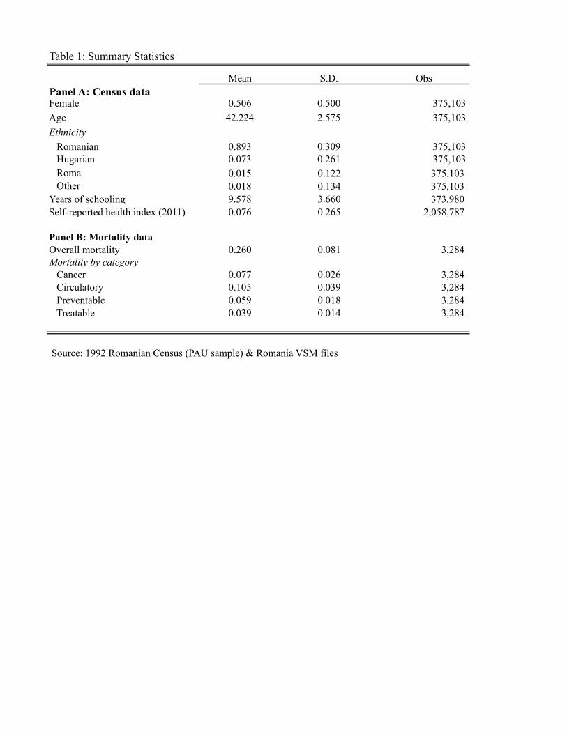
Table 1: Summary Statistics

Mean S.D. ObsPanel A: Census dataFemale 0.506 0.500 375,103 Age 42.224 2.575 375,103 Ethnicity Romanian 0.893 0.309 375,103 Hugarian 0.073 0.261 375,103 Roma 0.015 0.122 375,103 Other 0.018 0.134 375,103 Years of schooling 9.578 3.660 373,980 Self-reported health index (2011) 0.076 0.265 2,058,787

Panel B: Mortality dataOverall mortality 0.260 0.081 3,284 Mortality by category Cancer 0.077 0.026 3,284 Circulatory 0.105 0.039 3,284 Preventable 0.059 0.018 3,284 Treatable 0.039 0.014 3,284

Source: 1992 Romanian Census (PAU sample) & Romania VSM files

Table 2: Effects of the Educational Expansion on Years of Schooling

Bandwidth (days) 180 120 90 60 30 IK 180 120 90 60 30 IK

(1) (2) (3) (4) (5) (6) (7) (8) (9) (10) (11) (12)

0.209*** 0.299*** 0.395*** 0.517*** 0.669*** 0.644*** 0.104*** 0.160*** 0.242*** 0.336*** 0.329** 0.344***[0.048] [0.058] [0.067] [0.082] [0.124] [0.115] [0.039] [0.049] [0.059] [0.077] [0.125] [0.082]

Sample size 232,899 150,135 108,458 68,527 32,013 36,820 224,186 141,422 99,745 59,814 23,300 53,167

R-squared 0.020 0.019 0.019 0.018 0.018 0.018 0.020 0.019 0.019 0.018 0.016 0.017

-0.025 -0.005 0.030 0.062 0.079 0.073 -0.056 -0.042 -0.004 0.023 -0.094 0.016[0.049] [0.064] [0.078] [0.102] [0.156] [0.146] [0.045] [0.060] [0.074] [0.100] [0.172] [0.108]

Sample size 135,114 89,330 65,606 41,882 19,599 22,519 130,133 84,349 60,625 36,901 14,618 32,849

R-squared 0.001 0.001 0.001 0.000 0.000 0.000 0.001 0.001 0.000 0.000 0.000 0.000

-0.025 -0.005 0.030 0.062 0.079 0.073 -0.056 -0.042 -0.004 0.023 -0.094 0.016[0.049] [0.064] [0.078] [0.102] [0.156] [0.146] [0.045] [0.060] [0.074] [0.100] [0.172] [0.108]

0.234*** 0.304*** 0.365*** 0.455*** 0.590*** 0.572*** 0.160*** 0.202*** 0.246** 0.313** 0.423* 0.328**[0.056] [0.072] [0.085] [0.103] [0.126] [0.122] [0.057] [0.077] [0.096] [0.129] [0.214] [0.139]

Sample size 368,013 239,465 174,064 110,409 51,612 59,339 354,319 225,771 160,370 96,715 37,918 86,016R-squared 0.022 0.021 0.020 0.019 0.018 0.018 0.022 0.021 0.020 0.019 0.018 0.019

Notes: Heteroskedacticity-robust standard errors clustered by day of birth are in parentheses. ***, **, and * indicate statistical significance at the 1, 5, and 10 percent level respectively. After is an indicator for individuals born after January 1. Treatment is an indicator that equals 1 for cohorts who experienced an education expansion. The IK bandwidth is the Imbens and Kalyanarman (2012) optimal bandwidth.

Full sample Excluding 7 days on each side of cutoff

After

After

After

After*Treatment

Panel A: Treated years

Panel B: Control years

Panel C: All years

Table 3: Effects of Educational Expansion on Mortality Rate

Bandwidth (days) 180 120 90 60 30 IK 180 120 90 60 30 IK(1) (2) (3) (4) (5) (6) (7) (8) (9) (10) (11) (12)

0.010 0.006 0.003 0.003 -0.006 0.003 0.011 0.007 0.003 0.004 -0.016 0.011[0.009] [0.011] [0.013] [0.015] [0.016] [0.012] [0.010] [0.014] [0.018] [0.026] [0.053] [0.010]

Sample size 2,154 1,434 1,074 714 354 1,152 2,070 1,350 990 630 270 2,105

R-squared 0.118 0.112 0.105 0.108 0.130 0.106 0.124 0.119 0.113 0.118 0.147 0.124

-0.011 -0.012 -0.015 -0.020* -0.046*** -0.014 -0.002 0.004 0.006 0.013 -0.001 -0.002[0.007] [0.008] [0.009] [0.011] [0.015] [0.009] [0.007] [0.009] [0.010] [0.012] [0.022] [0.007]

Sample size 1,077 717 537 357 177 576 1,035 675 495 315 135 1,053

R-squared 0.071 0.073 0.079 0.082 0.146 0.078 0.058 0.055 0.055 0.046 0.042 0.059

-0.011 -0.012 -0.015 -0.020* -0.046*** -0.014 -0.002 0.004 0.006 0.013 -0.001 -0.002[0.007] [0.008] [0.009] [0.011] [0.015] [0.009] [0.007] [0.009] [0.010] [0.012] [0.022] [0.007]

0.021* 0.018 0.018 0.023 0.040* 0.017 0.013 0.003 -0.003 -0.009 -0.014 0.013[0.012] [0.014] [0.016] [0.019] [0.020] [0.016] [0.014] [0.018] [0.023] [0.032] [0.062] [0.013]

Sample size 3,231 2,151 1,611 1,071 531 1,728 3,105 2,025 1,485 945 405 3,158R-squared 0.253 0.242 0.232 0.219 0.223 0.234 0.261 0.252 0.242 0.229 0.228 0.261

Notes: Heteroskedacticity-robust standard errors clustered by day of birth are in parentheses. ***, **, and * indicate statistical significance at the 1, 5, and 10 percent level respectively. After is an indicator for individuals born after January 1. Treatment is an indicator that equals 1 for cohorts who experienced an education expansion. The IK bandwidth is the Imbens and Kalyanarman (2012) optimal bandwidth.

Full sample Excluding 7 days on each side of cutoff

Panel A: Treated years

After

Panel B: Control years

After

Panel C: All years

After

After*Treatment

Table 4: Effects of Educational Expansion on Mortality Rate due to Cancer

Bandwidth (days) 180 120 90 60 30 IK 180 120 90 60 30 IK

(1) (2) (3) (4) (5) (6) (7) (8) (9) (10) (11) (12)

0.001 0.001 -0.000 -0.001 -0.003 0.000 0.001 -0.000 -0.001 -0.002 -0.012 0.001[0.003] [0.004] [0.005] [0.005] [0.005] [0.004] [0.004] [0.005] [0.007] [0.010] [0.019] [0.004]

Sample size 2,154 1,434 1,074 714 354 1,248 2,070 1,350 990 630 270 2,105

R-squared 0.062 0.058 0.055 0.063 0.098 0.056 0.067 0.063 0.060 0.066 0.094 0.067

-0.003 -0.002 -0.003 -0.004 -0.014** -0.002 0.001 0.003 0.004 0.008 -0.000 0.000[0.002] [0.003] [0.004] [0.004] [0.006] [0.003] [0.003] [0.003] [0.004] [0.005] [0.009] [0.002]

Sample size 1,077 717 537 357 177 624 1,035 675 495 315 135 1,053

R-squared 0.049 0.047 0.049 0.049 0.104 0.048 0.039 0.036 0.035 0.028 0.022 0.040

-0.003 -0.002 -0.003 -0.004 -0.014** -0.002 0.001 0.003 0.004 0.008 -0.000 0.000[0.002] [0.003] [0.004] [0.004] [0.006] [0.003] [0.003] [0.003] [0.004] [0.005] [0.009] [0.002]

0.004 0.003 0.003 0.004 0.011 0.003 0.000 -0.003 -0.006 -0.010 -0.012 0.001[0.004] [0.006] [0.006] [0.008] [0.008] [0.006] [0.005] [0.007] [0.009] [0.013] [0.024] [0.005]

Sample size 3,231 2,151 1,611 1,071 531 1,872 3,105 2,025 1,485 945 405 3,158R-squared 0.167 0.160 0.153 0.145 0.163 0.157 0.174 0.169 0.162 0.152 0.158 0.174

After

After*Treatment

Notes: Heteroskedacticity-robust standard errors clustered by day of birth are in parentheses. ***, **, and * indicate statistical significance at the 1, 5, and 10 percent level respectively. After is an indicator for individuals born after January 1. Treatment is an indicator that equals 1 for cohorts who experienced an education expansion. The IK bandwidth is the Imbens and Kalyanarman (2012) optimal bandwidth. We use the ICD-10 diseases codes - chapter C for cancer.

Full sample Excluding 7 days on each side of cutoff

After

After

Panel A: Treated years

Panel B: Control years

Panel C: All years

Table 5: Effects of Educational Expansion on Mortality Rate due to Circulatory Diseases

Bandwidth (days) 180 120 90 60 30 IK 180 120 90 60 30 IK

(1) (2) (3) (4) (5) (6) (7) (8) (9) (10) (11) (12)

0.007** 0.005 0.003 0.002 -0.003 0.005 0.009** 0.007 0.005 0.006 0.005 0.009**[0.004] [0.004] [0.005] [0.006] [0.007] [0.004] [0.004] [0.006] [0.007] [0.010] [0.019] [0.004]

Sample size 2,154 1,434 1,074 714 354 1,530 2,070 1,350 990 630 270 1,974

R-squared 0.223 0.216 0.210 0.215 0.238 0.217 0.227 0.220 0.215 0.222 0.255 0.226

-0.003 -0.003 -0.004 -0.005 -0.012*** -0.003 -0.000 0.000 0.001 0.003 -0.004 -0.000[0.002] [0.003] [0.003] [0.003] [0.004] [0.003] [0.003] [0.004] [0.004] [0.005] [0.010] [0.003]

Sample size 1,077 717 537 357 177 765 1,035 675 495 315 135 987

R-squared 0.123 0.128 0.137 0.144 0.201 0.126 0.108 0.105 0.108 0.100 0.095 0.107

-0.003 -0.003 -0.004 -0.005 -0.012*** -0.003 -0.000 0.000 0.001 0.003 -0.004 -0.000[0.002] [0.003] [0.003] [0.003] [0.004] [0.003] [0.003] [0.004] [0.004] [0.005] [0.010] [0.003]

0.010** 0.008 0.007 0.007 0.009 0.008 0.010* 0.006 0.004 0.004 0.009 0.009*[0.004] [0.005] [0.006] [0.007] [0.007] [0.005] [0.005] [0.007] [0.008] [0.011] [0.020] [0.005]

Sample size 3,231 2,151 1,611 1,071 531 2,295 3,105 2,025 1,485 945 405 2,961R-squared 0.410 0.399 0.391 0.383 0.388 0.401 0.413 0.402 0.393 0.382 0.380 0.412

After

After*Treatment

Notes: Heteroskedacticity-robust standard errors clustered by day of birth are in parentheses. ***, **, and * indicate statistical significance at the 1, 5, and 10 percent level respectively. After is an indicator for individuals born after January 1. Treatment is an indicator that equals 1 for cohorts who experienced an education expansion. The IK bandwidth is the Imbens and Kalyanarman (2012) optimal bandwidth. We use the ICD-10 diseases codes- chapter I for the circulatory diseases.

Full sample Excluding 7 days on each side of cutoff

After

After

Panel A: Treated years

Panel B: Control years

Panel C: All years

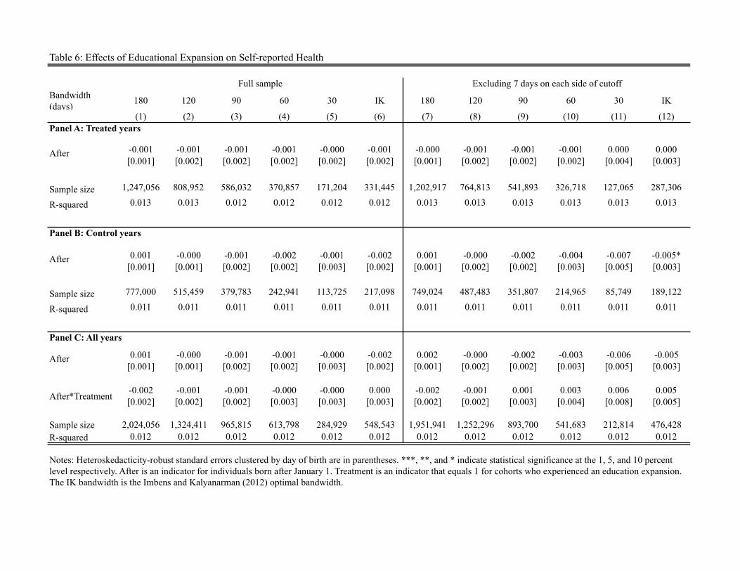
Table 6: Effects of Educational Expansion on Self-reported Health

Bandwidth (days) 180 120 90 60 30 IK 180 120 90 60 30 IK

(1) (2) (3) (4) (5) (6) (7) (8) (9) (10) (11) (12)

-0.001 -0.001 -0.001 -0.001 -0.000 -0.001 -0.000 -0.001 -0.001 -0.001 0.000 0.000[0.001] [0.002] [0.002] [0.002] [0.002] [0.002] [0.001] [0.002] [0.002] [0.002] [0.004] [0.003]

Sample size 1,247,056 808,952 586,032 370,857 171,204 331,445 1,202,917 764,813 541,893 326,718 127,065 287,306

R-squared 0.013 0.013 0.012 0.012 0.012 0.012 0.013 0.013 0.013 0.013 0.013 0.013

0.001 -0.000 -0.001 -0.002 -0.001 -0.002 0.001 -0.000 -0.002 -0.004 -0.007 -0.005*[0.001] [0.001] [0.002] [0.002] [0.003] [0.002] [0.001] [0.002] [0.002] [0.003] [0.005] [0.003]

Sample size 777,000 515,459 379,783 242,941 113,725 217,098 749,024 487,483 351,807 214,965 85,749 189,122

R-squared 0.011 0.011 0.011 0.011 0.011 0.011 0.011 0.011 0.011 0.011 0.011 0.011

0.001 -0.000 -0.001 -0.001 -0.000 -0.002 0.002 -0.000 -0.002 -0.003 -0.006 -0.005[0.001] [0.001] [0.002] [0.002] [0.003] [0.002] [0.001] [0.002] [0.002] [0.003] [0.005] [0.003]

-0.002 -0.001 -0.001 -0.000 -0.000 0.000 -0.002 -0.001 0.001 0.003 0.006 0.005[0.002] [0.002] [0.002] [0.003] [0.003] [0.003] [0.002] [0.002] [0.003] [0.004] [0.008] [0.005]

Sample size 2,024,056 1,324,411 965,815 613,798 284,929 548,543 1,951,941 1,252,296 893,700 541,683 212,814 476,428R-squared 0.012 0.012 0.012 0.012 0.012 0.012 0.012 0.012 0.012 0.012 0.012 0.012

After

After*Treatment

Notes: Heteroskedacticity-robust standard errors clustered by day of birth are in parentheses. ***, **, and * indicate statistical significance at the 1, 5, and 10 percent level respectively. After is an indicator for individuals born after January 1. Treatment is an indicator that equals 1 for cohorts who experienced an education expansion. The IK bandwidth is the Imbens and Kalyanarman (2012) optimal bandwidth.

Full sample Excluding 7 days on each side of cutoff

After

After

Panel A: Treated years

Panel B: Control years

Panel C: All years

Table 7: Effect of Educational Expansion on Employment

Bandwidth (days) 180 120 90 60 30 IK 180 120 90 60 30 IK

(1) (2) (3) (4) (5) (6) (7) (8) (9) (10) (11) (12)

0.010*** 0.017*** 0.021*** 0.027*** 0.037*** 0.034*** 0.003 0.008* 0.010* 0.015** 0.023 0.008*[0.004] [0.004] [0.005] [0.005] [0.007] [0.007] [0.003] [0.004] [0.005] [0.007] [0.015] [0.004]

Sample size 233,402 150,439 108,658 68,721 32,116 40,385 224,659 141,696 99,915 59,978 23,373 143,836R-squared 0.002 0.002 0.002 0.002 0.003 0.003 0.002 0.002 0.002 0.002 0.002 0.002

-0.005 0.001 0.007 0.011 0.022** 0.022** -0.009* -0.005 0.001 0.007 0.040* -0.005[0.005] [0.006] [0.006] [0.008] [0.010] [0.009] [0.005] [0.007] [0.008] [0.012] [0.020] [0.007]

Sample size 135,396 89,500 65,692 42,013 19,661 24,801 130,393 84,497 60,689 37,010 14,658 85,598R-squared 0.000 0.000 0.000 0.000 0.000 0.000 0.000 0.000 0.000 0.000 0.001 0.000

-0.005 0.001 0.007 0.011 0.022** 0.022** -0.009* -0.005 0.001 0.007 0.040* -0.005[0.005] [0.006] [0.006] [0.008] [0.010] [0.009] [0.005] [0.007] [0.008] [0.012] [0.020] [0.007]

0.015*** 0.016** 0.015* 0.016* 0.015 0.012 0.012** 0.013 0.009 0.008 -0.017 0.013[0.005] [0.007] [0.008] [0.009] [0.012] [0.011] [0.006] [0.008] [0.010] [0.014] [0.026] [0.008]

Sample size 368,798 239,939 174,350 110,734 51,777 65,186 355,052 226,193 160,604 96,988 38,031 229,434R-squared 0.002 0.002 0.002 0.002 0.003 0.002 0.002 0.002 0.002 0.002 0.002 0.002

After

After*Treatment

Notes: Heteroskedacticity-robust standard errors clustered by day of birth are in parentheses. ***, **, and * indicate statistical significance at the 1, 5, and 10 percent level respectively. After is an indicator for individuals born after January 1. Treatment is an indicator that equals 1 for cohorts who experienced an education expansion. The IK bandwidth is the Imbens and Kalyanarman (2012) optimal bandwidth.

Full sample Excluding 7 days on each side of cutoff

After

After

Panel A: Treated years

Panel B: Control years

Panel C: All years

APPENDIX FIGURE 1: Density checkNotes: Panels A and B are restricted to individuals born in the treatment years (1944-1950). Panels C and D are restricted to individuals born in the control years (1950-1953). Panels E and F are restricted to individuals born in both treatment and control years (1944-1953). The open circles indicate the mean of the outcome by day of birth (panels A, C and E) or week of birth (panels B, D and F). The solid lines are fitted values of residuals from local linear regressions of the dependent variable. Source: 1992 Romanian Census (PAU sample).

0.0

1de

nsity

-180 0 180day of birth

Panel A: Treatment

0.0

1de

nsity

-26 0 26week of birth

Panel B: Treatment0

.01

dens

ity

-180 0 180day of birth

Panel C: Control

0.0

1de

nsity

-26 0 26week of birth

Panel D: Control

-.001

.001

dens

ity

-180 0 180day of birth

Panel E: Treatment-Control

-.001

.001

dens

ity

-26 0 26week of birth

Panel F: Treatment-Control

APPENDIX FIGURE 2: Mortality Rate due to CancerNotes: Panels A and B are restricted to individuals born in the treatment years (1944-1950). Panels C and D are restricted to individuals born in the control years (1950-1953). Panels E and F are restricted to individuals born in both treatment and control years (1944-1953). The open circles indicate the mean of the outcome by day of birth (panels A, C and E) or week of birth (panels B, D and F). The solid lines are fitted values of residuals from local linear regressions of the dependent variable. Source: 1994-2011 Vital Statistics Mortality files

0.2

Mor

talit

y R

ate

-180 0 180day of birth

Panel A: Treatment

0.2

Mor

talit

y R

ate

-26 0 26week of birth

Panel B: Treatment-.0

5.1

5M

orta

lity

Rat

e

-180 0 180day of birth

Panel C: Control

-.05

.15

Mor

talit

y R

ate

-26 0 26week of birth

Panel D: Control

-.05

.15

Mor

talit

y R

ate

-180 0 180day of birth

Panel E: Treatment-Control

-.05

.15

Mor

talit

y R

ate

-26 0 26week of birth

Panel F: Treatment-Control

APPENDIX FIGURE 3: Mortality Rate due to Circulatory DiseasesNotes: Panels A and B are restricted to individuals born in the treatment years (1944-1950). Panels C and D are restricted to individuals born in the control years (1950-1953). Panels E and F are restricted to individuals born in both treatment and control years (1944-1953). The open circles indicate the mean of the outcome by day of birth (panels A, C and E) or week of birth (panels B, D and F). The solid lines are fitted values of residuals from local linear regressions of the dependent variable. Source: 1994-2011 Vital Statistics Mortality files

0.2

Mor

talit

y R

ate

-180 0 180day of birth

Panel A: Treatment

0.2

Mor

talit

y R

ate

-26 0 26week of birth

Panel B: Treatment-.0

5.1

5M

orta

lity

Rat

e

-180 0 180day of birth

Panel C: Control

-.05

.15

Mor

talit

y R

ate

-26 0 26week of birth

Panel D: Control

-.05

.15

Mor

talit

y R

ate

-180 0 180day of birth

Panel E: Treatment-Control

-.05

.15

Mor

talit

y R

ate

-26 0 26week of birth

Panel F: Treatment-Control

APPENDIX FIGURE 4:Self-Reported Health IndexNotes: Panels A and B are restricted to individuals born in the treatment years (1944-1950). Panels C and D are restricted to individuals born in the control years (1950-1953). Panels E and F are restricted to individuals born in both treatment and control years (1944-1953). The open circles indicate the mean of the outcome by day of birth (panels A, C and E) or week of birth (panels B, D and F). The solid lines are fitted values of residuals from local linear regressions of the dependent variable. Source: 2011 Romanian Census

0.1

Hea

lth In

dex

-180 0 180day of birth

Panel A: Treatment

0.1

Hea

lth In

dex

-26 0 26week of birth

Panel B: Treatment0

.1H

ealth

Inde

x

-180 0 180day of birth

Panel C: Control

0.1

Hea

lth In

dex

-26 0 26week of birth

Panel D: Control

-.05

.05

Hea

lth

-180 0 180day of birth

Panel E: Treatment-Control

-.05

.05

Hea

lth In

dex

-26 0 26week of birth

Panel F: Treatment-Control

APPENDIX FIGURE 5: Rate of EmploymentNotes: Panels A and B are restricted to individuals born in the treatment years (1944-1950). Panels C and D are restricted to individuals born in the control years (1950-1953). Panels E and F are restricted to individuals born in both treatment and control years (1944-1953). The open circles indicate the mean of the outcome by day of birth (panels A, C and E) or week of birth (panels B, D and F). The solid lines are fitted values of residuals from local linear regressions of the dependent variable. Source: 1992 Romanian Census (PAU sample).

.7.9

fract

ion

empl

oyed

loye

d

-180 0 180day of birth

Panel A: Treatment

.7.9

fract

ion

empl

oyed

loye

d-26 0 26

week of birth

Panel B: Treatment.7

.9fra

ctio

n em

ploy

edlo

yed

-180 0 180day of birth

Panel C: Control

.7.9

fract

ion

empl

oyed

loye

d

-26 0 26week of birth

Panel D: Control

-.1.1

fract

ion

empl

oyed

loye

d

-180 0 180day of birth

Panel E: Treatment-Control

-.1.1

fract

ion

empl

oyed

loye

d

-26 0 26week of birth

Panel F: Treatment-Control

Appendix Table 1: Density Checks

Bandwidth (days) 180 120 90 60 30 IK 180 120 90 60 30 IK

(1) (2) (3) (4) (5) (6) (7) (8) (9) (10) (11) (12)

0.167** 0.224** 0.262** 0.337** 0.519*** 1.005*** 0.064*** 0.072*** 0.060*** 0.049*** 0.076*** -[0.073] [0.100] [0.122] [0.150] [0.179] [0.119] [0.011] [0.013] [0.013] [0.011] [0.018] -

Sample size 233,596 150,586 108,797 68,738 32,116 8,743 224,853 141,843 100,054 59,995 23,373 -R-squared 0.139 0.188 0.227 0.305 0.502 0.843 0.210 0.284 0.312 0.352 0.473 -

0.134*** 0.174** 0.200** 0.249** 0.388** 0.823*** 0.069*** 0.078*** 0.069*** 0.055*** 0.067** -[0.050] [0.070] [0.088] [0.114] [0.148] [0.111] [0.010] [0.011] [0.012] [0.012] [0.026] -

Sample size 135,524 89,614 65,819 42,014 19,661 5,003 130,521 84,611 60,816 37,011 14,658 -R-squared 0.157 0.199 0.223 0.280 0.455 0.828 0.172 0.286 0.337 0.405 0.446 -

0.134*** 0.174** 0.200** 0.249** 0.388** 0.823*** 0.069*** 0.078*** 0.069*** 0.055*** 0.067** -[0.050] [0.070] [0.088] [0.114] [0.148] [0.111] [0.010] [0.011] [0.012] [0.012] [0.026] -

0.033 0.050 0.063* 0.088** 0.131*** 0.182*** -0.005 -0.006 -0.009 -0.006 0.009 -[0.024] [0.030] [0.034] [0.037] [0.032] [0.012] [0.006] [0.007] [0.008] [0.010] [0.018] -

Sample size 369,120 240,200 174,616 110,752 51,777 13,746 355,374 226,454 160,870 97,006 38,031 -R-squared 0.144 0.191 0.226 0.299 0.492 0.842 0.199 0.288 0.326 0.378 0.481 -

After

After*Treatment

Notes: Heteroskedacticity-robust standard errors clustered by day of birth are in parentheses. ***, **, and * indicate statistical significance at the 1, 5, and 10 percent level respectively. After is an indicator for individuals born after January 1. Treatment is an indicator that equals 1 for cohorts who experienced an education expansion. The IK bandwidth is the Imbens and Kalyanarman (2012) optimal bandwidth. Coefficients are multuplied by 100 for clarity. The IK bandwidth when excluding 7 days on each side of the cutoff is less than 7 days so these estimates are missing.

Full sample Excluding 7 days on each side of cutoff

After

After

Panel A: Treated years

Panel B: Control years

Panel C: All years

Appendix Table 2: Specification Tests for Covariates (1)

bandwidth (days) 180 120 90 60 30 IK 180 120 90 60 30 IK(1) (2) (3) (4) (5) (6) (1) (2) (3) (4) (5) (6)

Female-0.025*** -0.038*** -0.050*** -0.073*** -0.104*** -0.104*** -0.009 -0.016 -0.023* -0.047*** -0.101*** -0.036**

[0.009] [0.012] [0.014] [0.017] [0.022] [0.022] [0.008] [0.010] [0.012] [0.016] [0.025] [0.014]

-0.013 -0.022** -0.028** -0.024* -0.026 -0.026 -0.006 -0.012 -0.016 -0.002 0.050 -0.012[0.008] [0.010] [0.011] [0.014] [0.020] [0.020] [0.009] [0.012] [0.014] [0.019] [0.031] [0.017]

Sample size 368,798 239,939 174,350 110,734 51,777 51,777 355,052 226,193 160,604 96,988 38,031 115,133

R-squared 0.001 0.001 0.002 0.003 0.006 0.006 0.000 0.001 0.001 0.001 0.002 0.001

Ethnic Romanian0.015*** 0.024*** 0.029*** 0.032*** 0.033*** 0.032*** 0.013** 0.023*** 0.029*** 0.031*** 0.022 0.032***[0.005] [0.006] [0.006] [0.007] [0.011] [0.008] [0.005] [0.007] [0.008] [0.011] [0.022] [0.010]

-0.008 -0.011 -0.012 -0.012 -0.007 -0.010 -0.009 -0.014* -0.017** -0.019* -0.007 -0.019*[0.005] [0.007] [0.008] [0.010] [0.014] [0.011] [0.005] [0.007] [0.008] [0.011] [0.021] [0.010]

Sample size 368,798 239,939 174,350 110,734 51,777 90,026 355,052 226,193 160,604 96,988 38,031 109,578

R-squared 0.001 0.001 0.001 0.001 0.002 0.001 0.001 0.001 0.001 0.001 0.001 0.001

Ethnic Hungarian-0.013*** -0.019*** -0.021*** -0.023*** -0.022*** -0.023*** -0.013*** -0.020*** -0.024*** -0.027*** -0.020 -0.026***

[0.003] [0.004] [0.005] [0.005] [0.007] [0.006] [0.004] [0.005] [0.006] [0.008] [0.015] [0.007]

0.006 0.009 0.010 0.012 0.011 0.012 0.005 0.010 0.013 0.018* 0.006 0.015*[0.004] [0.006] [0.007] [0.008] [0.012] [0.008] [0.005] [0.006] [0.008] [0.011] [0.019] [0.009]

Sample size 368,798 239,939 174,350 110,734 51,777 104,061 355,052 226,193 160,604 96,988 38,031 128,744R-squared 0.001 0.001 0.001 0.001 0.001 0.001 0.001 0.001 0.001 0.002 0.001 0.001

After

After*Treatment

After

After*Treatment

Notes: Heteroskedacticity-robust standard errors clustered by day of birth are in parentheses. ***, **, and * indicate statistical significance at the 1, 5, and 10 percent level respectively. After is an indicator for individuals born after January 1. Treatment is an indicator that equals 1 for cohorts who experienced an education expansion. The IK bandwidth is the Imbens and Kalyanarman (2012) optimal bandwidth.

After*Treatment

dependent variable: years of schoolingFull sample Excluding 7 days on each side of cutoff

After

Appendix Table 3: Specification Tests for Covariates (2)

bandwidth (days) 180 120 90 60 30 IK 180 120 90 60 30 IK(1) (2) (3) (4) (5) (6) (1) (2) (3) (4) (5) (6)

Ethnic Roma-0.000 -0.002 -0.004 -0.004 -0.005 -0.004 0.001 -0.001 -0.003 -0.002 0.006 -0.002[0.002] [0.002] [0.003] [0.003] [0.005] [0.003] [0.002] [0.003] [0.003] [0.004] [0.008] [0.004]

0.001 0.000 0.000 -0.001 -0.005 -0.002 0.002 0.001 0.001 -0.002 -0.012* -0.002[0.002] [0.003] [0.003] [0.005] [0.008] [0.005] [0.002] [0.003] [0.003] [0.004] [0.006] [0.004]

Sample size 368,798 239,939 174,350 110,734 51,777 105,028 355,052 226,193 160,604 96,988 38,031 105,506

R-squared 0.000 0.001 0.001 0.001 0.001 0.001 0.000 0.000 0.000 0.000 0.001 0.000

Ethnic Other-0.002 -0.004* -0.004* -0.004 -0.006 -0.004* -0.001 -0.002 -0.003 -0.002 -0.008 -0.001[0.002] [0.002] [0.003] [0.003] [0.004] [0.002] [0.002] [0.003] [0.003] [0.005] [0.011] [0.002]

0.001 0.002 0.002 0.001 0.001 0.002 0.002 0.003 0.003 0.003 0.013 0.001[0.002] [0.003] [0.003] [0.004] [0.006] [0.003] [0.002] [0.003] [0.004] [0.005] [0.010] [0.002]

Sample size 368,798 239,939 174,350 110,734 51,777 238,075 355,052 226,193 160,604 96,988 38,031 360,792

R-squared 0.000 0.000 0.000 0.000 0.000 0.000 0.000 0.000 0.000 0.000 0.000 0.000

Born in Bucharest-0.009*** -0.011*** -0.012*** -0.011** -0.014** -0.012** -0.008*** -0.010*** -0.010** -0.006 -0.006 -0.009***

[0.003] [0.003] [0.004] [0.005] [0.007] [0.005] [0.003] [0.004] [0.004] [0.006] [0.012] [0.003]

0.002 0.003 0.003 0.001 0.003 0.001 0.004 0.005 0.005 0.002 0.009 0.004[0.003] [0.004] [0.005] [0.006] [0.009] [0.006] [0.003] [0.004] [0.005] [0.008] [0.016] [0.004]

Sample size 368,798 239,939 174,350 110,734 51,777 115,361 355,052 226,193 160,604 96,988 38,031 279,260R-squared 0 0 0.001 0.001 0.001 0.001 0 0 0 0.001 0.001 0

After

After*Treatment

After

After*Treatment

Notes: Heteroskedacticity-robust standard errors clustered by day of birth are in parentheses. ***, **, and * indicate statistical significance at the 1, 5, and 10 percent level respectively. After is an indicator for individuals born after January 1. Treatment is an indicator that equals 1 for cohorts who experienced an education expansion. The IK bandwidth is the Imbens and Kalyanarman (2012) optimal bandwidth.

After*Treatment

dependent variable: years of schoolingFull sample Excluding 7 days on each side of cutoff

After

Appendix Table 4: Effects of Educational Expansion on Actual Years of Schooling

Bandwidth (months) 6 5 4 3 2 6 5 4 3 2

(1) (2) (3) (4) (5) (7) (8) (9) (10) (11)

0.291 0.550** 0.641** 0.981*** 1.183*** 0.175 0.356* 0.495*** 0.601*** 0.837***[0.275] [0.212] [0.197] [0.149] [0.020] [0.225] [0.189] [0.126] [0.098] [0.014]

Sample size 5,294 4,376 3,439 2,526 1,596 8,383 6,909 5,416 3,909 2,421R-squared 0.017 0.018 0.017 0.017 0.019 0.027 0.029 0.032 0.032 0.029

0.107 0.455 0.471** 0.565*** 0.724*** -0.029 -0.110 -0.156 0.155** 0.129***[0.321] [0.268] [0.172] [0.111] [0.025] [0.194] [0.151] [0.250] [0.044] [0.004]

Sample size 2,356 1,968 1,550 1,143 690 4,887 4,068 3,209 2,377 1,498R-squared 0.001 0.001 0.004 0.007 0.006 0.004 0.006 0.003 0.006 0.003

0.107 0.455 0.471** 0.565*** 0.724*** -0.029 -0.110 -0.156 0.155** 0.129***[0.321] [0.268] [0.172] [0.111] [0.025] [0.194] [0.151] [0.250] [0.044] [0.004]

0.184 0.095 0.169 0.416 0.458*** 0.204 0.466** 0.651** 0.446*** 0.708***[0.267] [0.270] [0.197] [0.210] [0.033] [0.184] [0.167] [0.220] [0.102] [0.013]

Sample size 7,650 6,344 4,989 3,669 2,286 13,270 10,977 8,625 6,286 3,919R-squared 0.040 0.042 0.046 0.050 0.044 0.041 0.043 0.046 0.043 0.042

Notes: Heteroskedacticity-robust standard errors clustered by day of birth are in parentheses. ***, **, and * indicate statistical significance at the 1, 5, and 10 percent level respectively. After is an indicator for individuals born after January 1. Treatment is an indicator that equals 1 for cohorts who experienced an education expansion. The IK bandwidth is the Imbens and Kalyanarman (2012) optimal bandwidth.

After

After*Treatment

1994 LSMS 1995-96 LSMS

After

After

Panel A: Treated years

Panel B: Control years

Panel C: All years

Appendix Table 5: Effects of Educational Expansion on Mortality Rate due to Preventable Diseases

Bandwidth (days) 180 120 90 60 30 IK 180 120 90 60 30 IK

(1) (2) (3) (4) (5) (6) (7) (8) (9) (10) (11) (12)

0.000 -0.000 -0.001 -0.001 -0.003 -0.001 0.001 0.000 -0.000 0.000 -0.003 0.000[0.002] [0.003] [0.003] [0.003] [0.004] [0.003] [0.002] [0.003] [0.004] [0.006] [0.012] [0.002]

Sample size 2,154 1,434 1,074 714 354 1,236 2,070 1,350 990 630 270 2,105

R-squared 0.023 0.022 0.020 0.024 0.047 0.021 0.025 0.026 0.025 0.031 0.056 0.025

-0.002 -0.002 -0.002 -0.003 -0.010* -0.002 -0.000 0.002 0.003 0.005 0.002 -0.001[0.002] [0.003] [0.003] [0.004] [0.006] [0.003] [0.002] [0.003] [0.003] [0.003] [0.006] [0.002]

Sample size 1,077 717 537 357 177 618 1,035 675 495 315 135 1,053

R-squared 0.025 0.025 0.026 0.027 0.067 0.026 0.019 0.021 0.021 0.017 0.016 0.021

-0.002 -0.002 -0.002 -0.003 -0.010* -0.002 -0.000 0.002 0.003 0.005 0.002 -0.001[0.002] [0.003] [0.003] [0.004] [0.006] [0.003] [0.002] [0.003] [0.003] [0.003] [0.006] [0.002]

0.002 0.001 0.001 0.002 0.007 0.001 0.001 -0.002 -0.004 -0.005 -0.005 0.001[0.003] [0.004] [0.004] [0.005] [0.006] [0.004] [0.003] [0.005] [0.006] [0.008] [0.014] [0.003]

Sample size 3,231 2,151 1,611 1,071 531 1,854 3,105 2,025 1,485 945 405 3,158R-squared 0.057 0.056 0.051 0.049 0.070 0.053 0.061 0.061 0.058 0.055 0.070 0.059

After

After*Treatment

Notes: Heteroskedacticity-robust standard errors clustered by day of birth are in parentheses. ***, **, and * indicate statistical significance at the 1, 5, and 10 percent level respectively. After is an indicator for individuals born after January 1. Treatment is an indicator that equals 1 for cohorts who experienced an education expansion. The IK bandwidth is the Imbens and Kalyanarman (2012) optimal bandwidth. The preventable causes of death include: Lung cancer (C33-C34), Cirrhosis of liver (K70, K74.3-K74.6), External causes of death (V, W, X, Y).

Full sample Excluding 7 days on each side of cutoff

After

After

Panel A: Treated years

Panel B: Control years

Panel C: All years

Appendix Table 6: Effects of Educational Expansion on Mortality Rate due to Treatable Diseases

Bandwidth (days) 180 120 90 60 30 IK 180 120 90 60 30 IK

(1) (2) (3) (4) (5) (6) (7) (8) (9) (10) (11) (12)

0.002 0.001 -0.000 -0.001 -0.003 0.001 0.002 0.002 0.001 0.001 -0.002 0.002[0.002] [0.002] [0.002] [0.002] [0.003] [0.002] [0.002] [0.002] [0.003] [0.004] [0.008] [0.002]

Sample size 2,154 1,434 1,074 714 354 1,638 2,070 1,350 990 630 270 1,974

R-squared 0.106 0.102 0.095 0.096 0.101 0.103 0.111 0.108 0.103 0.109 0.133 0.110

-0.002 -0.002 -0.003** -0.004** -0.007*** -0.002 -0.000 -0.000 -0.001 0.001 0.001 -0.000[0.001] [0.001] [0.002] [0.002] [0.002] [0.001] [0.001] [0.002] [0.002] [0.002] [0.005] [0.001]

Sample size 1,077 717 537 357 177 819 1,035 675 495 315 135 987

R-squared 0.045 0.045 0.051 0.055 0.094 0.043 0.038 0.031 0.031 0.027 0.026 0.037

-0.002 -0.002 -0.003** -0.004** -0.007*** -0.002 -0.000 -0.000 -0.001 0.001 0.001 -0.000[0.001] [0.001] [0.002] [0.002] [0.002] [0.001] [0.001] [0.002] [0.002] [0.002] [0.005] [0.001]

0.003 0.003 0.003 0.003 0.004 0.003 0.003 0.002 0.002 0.001 -0.003 0.002[0.002] [0.002] [0.003] [0.003] [0.004] [0.002] [0.002] [0.003] [0.004] [0.005] [0.011] [0.003]

Sample size 3,231 2,151 1,611 1,071 531 2,457 3,105 2,025 1,485 945 405 2,961R-squared 0.224 0.218 0.211 0.200 0.191 0.220 0.228 0.224 0.216 0.208 0.201 0.228

After

After*Treatment

Notes: Heteroskedacticity-robust standard errors clustered by day of birth are in parentheses. ***, **, and * indicate statistical significance at the 1, 5, and 10 percent level respectively. After is an indicator for individuals born after January 1. Treatment is an indicator that equals 1 for cohorts who experienced an education expansion. The IK bandwidth is the Imbens and Kalyanarman (2012) optimal bandwidth. Treatable causes of death (cf. ICD 10) include: Tuberculosis (A15-A19. B90), Malignant neoplasm of cervix uteri (C53); Chronic rheumatic heart disease (I05-I09); All respiratory diseases (J00-J99); Asthma (J45, J46); Appendicitis (K35-K38); Abdominal hernia (K40-K46); Hypertensive and cerebrovascular disease (I10-I15, I60-I69); Chollelthiasis and cholecystitis (K80-K81).

Full sample Excluding 7 days on each side of cutoff

After

After

Panel A: Treated years

Panel B: Control years

Panel C: All years

Appendix Table 7: Effect of Educational Expansion on Fertility

bandwidth (days) 180 120 90 60 30 IK 180 120 90 60 30 IK(1) (2) (3) (4) (5) (6) (1) (2) (3) (4) (5) (6)

Treated years

-0.034 -0.061** -0.089*** -0.118*** -0.119*** -0.120*** -0.012 -0.035 -0.068 -0.110 -0.132 -0.113[0.023] [0.027] [0.030] [0.033] [0.032] [0.034] [0.027] [0.037] [0.047] [0.067] [0.138] [0.071]

Sample size 119,118 76,505 55,473 35,243 16,431 28,114 114,832 72,219 51,187 30,957 12,145 29,171R-squared 0.001 0.001 0.001 0.001 0.001 0.001 0.001 0.000 0.000 0.000 0.001 0.000

Control years0.048 0.084* 0.096* 0.123* 0.171* 0.150** 0.027 0.062 0.068 0.091 0.255 0.100

[0.036] [0.046] [0.054] [0.065] [0.088] [0.072] [0.039] [0.054] [0.069] [0.099] [0.212] [0.104]

Sample size 67,719 44,737 32,800 20,860 9,724 16,608 65,295 42,313 30,376 18,436 7,300 17,400R-squared 0.001 0.001 0.001 0.001 0.002 0.002 0.001 0.001 0.001 0.001 0.002 0.001

All years0.048 0.084* 0.096* 0.123* 0.171* 0.150** 0.027 0.062 0.068 0.091 0.255 0.100

[0.036] [0.046] [0.054] [0.065] [0.088] [0.072] [0.039] [0.054] [0.069] [0.099] [0.212] [0.104]

-0.082** -0.145*** -0.185*** -0.241*** -0.290*** -0.270*** -0.039 -0.097* -0.136* -0.201* -0.388* -0.214*[0.038] [0.047] [0.055] [0.065] [0.088] [0.072] [0.042] [0.056] [0.072] [0.103] [0.222] [0.109]

Sample size 186,837 121,242 88,273 56,103 26,155 44,722 180,127 114,532 81,563 49,393 19,445 46,571R-squared 0.001 0.001 0.001 0.001 0.001 0.001 0.001 0.001 0.001 0.001 0.002 0.001

After

After*Treatment

Notes: Heteroskedacticity-robust standard errors clustered by day of birth are in parentheses. ***, **, and * indicate statistical significance at the 1, 5, and 10 percent level respectively. After is an indicator for individuals born after January 1. Treatment is an indicator that equals 1 for cohorts who experienced an education expansion. The IK bandwidth is the Imbens and Kalyanarman (2012) optimal bandwidth.

dependent variable: number of childrenFull sample Excluding 7 days on each side of cutoff

After

After

Appendix Table 8: Effect of Educational Expansion on International Migration in the 2011 census

bandwidth (days) 180 120 90 60 30 IK 180 120 90 60 30 IK(1) (2) (3) (4) (5) (6) (1) (2) (3) (4) (5) (6)

Treated years

-0.000 -0.000 -0.000 -0.001 0.000 -0.000 -0.001* -0.001** -0.001* -0.001** -0.001 -0.001*[0.000] [0.000] [0.000] [0.001] [0.001] [0.000] [0.000] [0.000] [0.000] [0.001] [0.001] [0.000]

Sample size 2,170 1,448 1,085 718 354 1,430 2,086 1,364 1,001 634 270 1,672

R-squared 0.182 0.191 0.195 0.197 0.202 0.191 0.176 0.182 0.184 0.181 0.168 0.178

Control years

-0.000 -0.000 -0.001 -0.001 -0.002** -0.000 0.000 0.000 0.000 0.001 -0.001 0.000[0.001] [0.001] [0.001] [0.001] [0.001] [0.001] [0.001] [0.001] [0.001] [0.001] [0.001] [0.001]

Sample size 1,080 719 538 357 177 710 1,038 677 496 315 135 831

R-squared 0.090 0.096 0.096 0.089 0.119 0.096 0.099 0.105 0.104 0.105 0.133 0.101

All years

-0.000 -0.000 -0.001 -0.001 -0.002** -0.000 0.000 0.000 0.000 0.001 -0.001 0.000[0.001] [0.001] [0.001] [0.001] [0.001] [0.001] [0.001] [0.001] [0.001] [0.001] [0.001] [0.001]

-0.000 -0.000 0.000 0.000 0.002** -0.000 -0.001 -0.001 -0.001 -0.002* 0.000 -0.001[0.001] [0.001] [0.001] [0.001] [0.001] [0.001] [0.001] [0.001] [0.001] [0.001] [0.002] [0.001]

Sample size 3,250 2,167 1,623 1,075 531 2,140 3,124 2,041 1,497 949 405 2,503R-squared 0.364 0.367 0.371 0.382 0.420 0.367 0.355 0.351 0.348 0.351 0.353 0.352

After

After*Treatment

Notes: Heteroskedacticity-robust standard errors clustered by day of birth are in parentheses. ***, **, and * indicate statistical significance at the 1, 5, and 10 percent level respectively. After is an indicator for individuals born after January 1. Treatment is an indicator that equals 1 for cohorts who experienced an education expansion. The IK bandwidth is the Imbens and Kalyanarman (2012) optimal bandwidth.

dependent variable: migration rateFull sample Excluding 7 days on each side of cutoff

After

After

Appendix Table 9: Effect of Educational Expansion on Attrition between the 1992 and 2011 census

bandwidth (days) 180 120 90 60 30 IK 180 120 90 60 30 IK(1) (2) (3) (4) (5) (6) (1) (2) (3) (4) (5) (6)

Treated years

-0.008 -0.017 -0.020 -0.015 -0.026 -0.020 -0.012 -0.027 -0.035 -0.033 -0.102 -0.018[0.025] [0.031] [0.035] [0.040] [0.043] [0.036] [0.029] [0.040] [0.051] [0.073] [0.151] [0.034]

Sample size 2,155 1,435 1,075 714 354 1,045 2,071 1,351 991 630 270 1,645

R-squared 0.017 0.023 0.030 0.038 0.075 0.031 0.014 0.015 0.017 0.019 0.049 0.014

Control years

-0.058** -0.060* -0.064* -0.071* -0.156*** -0.065* -0.031 -0.016 -0.003 0.034 -0.037 -0.023[0.026] [0.031] [0.035] [0.039] [0.054] [0.035] [0.029] [0.036] [0.041] [0.045] [0.084] [0.033]

Sample size 1,078 718 538 357 177 523 1,036 676 496 315 135 823

R-squared 0.015 0.023 0.027 0.023 0.061 0.027 0.010 0.017 0.021 0.015 0.010 0.014

All years

-0.058** -0.060* -0.064* -0.071* -0.156*** -0.065* -0.031 -0.016 -0.003 0.034 -0.037 -0.023[0.026] [0.031] [0.035] [0.039] [0.054] [0.035] [0.029] [0.036] [0.041] [0.045] [0.084] [0.033]

0.050 0.043 0.044 0.057 0.130** 0.045 0.019 -0.011 -0.032 -0.067 -0.065 0.005[0.039] [0.047] [0.053] [0.059] [0.060] [0.053] [0.045] [0.060] [0.074] [0.100] [0.198] [0.052]

Sample size 3,233 2,153 1,613 1,071 531 1,568 3,107 2,027 1,487 945 405 2,468R-squared 0.022 0.028 0.036 0.045 0.088 0.037 0.016 0.018 0.022 0.023 0.043 0.017

After

After*Treatment

Notes: Heteroskedacticity-robust standard errors clustered by day of birth are in parentheses. ***, **, and * indicate statistical significance at the 1, 5, and 10 percent level respectively. After is an indicator for individuals born after January 1. Treatment is an indicator that equals 1 for cohorts who experienced an education expansion. The IK bandwidth is the Imbens and Kalyanarman (2012) optimal bandwidth.

dependent variable: attrition rateFull sample Excluding 7 days on each side of cutoff

After

After

Appendix Table 10: Effects of Educational Expansion on Employment and Income in the 1995-2000 LSMS data

Bandwidth (months) 6 5 4 3 2 6 5 4 3 2

(1) (2) (3) (4) (5) (7) (8) (9) (10) (11)

-0.0006 0.0127 0.0188* 0.0227* 0.0341*** -0.0130 0.0079 0.0122 0.0299 0.0675***[0.0120] [0.0096] [0.0094] [0.0096] [0.0011] [0.0260] [0.0232] [0.0266] [0.0209] [0.0009]

Sample size 40,558 33,512 26,211 19,089 12,005 40,234 33,245 26,012 18,955 11,920R-squared 0.016 0.016 0.015 0.014 0.013 0.010 0.010 0.010 0.009 0.010

-0.0239* -0.0132 -0.0224 -0.0188 -0.0131*** -0.0337 -0.0275 -0.0286 0.0105 0.0905***[0.0111] [0.0112] [0.0143] [0.0130] [0.0015] [0.0412] [0.0426] [0.0506] [0.0438] [0.0021]

Sample size 23,158 19,268 15,220 11,251 7,129 22,999 19,140 15,119 11,178 7,092R-squared 0.001 0.001 0.001 0.001 0.001 0.001 0.002 0.001 0.002 0.004

-0.0239* -0.0132 -0.0224 -0.0188 -0.0131*** -0.0337 -0.0275 -0.0286 0.0105 0.0905***[0.0111] [0.0112] [0.0143] [0.0130] [0.0015] [0.0412] [0.0426] [0.0506] [0.0438] [0.0021]

0.0234*** 0.0259** 0.0412*** 0.0415*** 0.0473*** 0.0207 0.0355 0.0408 0.0195 -0.0230***[0.0070] [0.0082] [0.0064] [0.0044] [0.0018] [0.0202] [0.0217] [0.0282] [0.0229] [0.0013]

Sample size 63,716 52,780 41,431 30,340 19,134 63,233 52,385 41,131 30,133 19,012R-squared 0.021 0.021 0.020 0.020 0.019 0.010 0.010 0.010 0.009 0.011

Notes: Heteroskedacticity-robust standard errors clustered by day of birth are in parentheses. ***, **, and * indicate statistical significance at the 1, 5, and 10 percent level respectively. After is an indicator for individuals born after January 1. Treatment is an indicator that equals 1 for cohorts who experienced an education expansion.

Employment Log Income

Panel A: Treated years

After

Panel B: Control years

After

Panel C: All years

After

After*Treatment

Appendix Table 11: Effect of Educational Expansion on Smoking and Chronic Conditions

Bandwidth (months) 6 5 4 3 2 6 5 4 3 2

(1) (2) (3) (4) (5) (6) (7) (8) (9) (10)

0.0092* 0.0092* 0.0095** 0.0117** 0.0067 0.0099** 0.0101* 0.0107* 0.0116* 0.0151**[0.0051] [0.0044] [0.0040] [0.0041] [0.0045] [0.0044] [0.0050] [0.0054] [0.0054] [0.0050]

Sample size

R-squared 113,367 94,611 73,720 53,302 32,486 113,367 94,611 73,720 53,302 32,486

0.003 0.003 0.003 0.003 0.003 0.001 0.001 0.001 0.001 0.001

0.0017 -0.0006 0.0007 0.0031 -0.0004 0.0017 0.0016 0.0040 0.0032 0.0087[0.0060] [0.0064] [0.0071] [0.0058] [0.0030] [0.0063] [0.0060] [0.0051] [0.0047] [0.0054]

Sample size

R-squared 64,852 54,126 42,289 30,730 19,048 64,852 54,126 42,289 30,730 19,048

0.001 0.001 0.001 0.001 0.001 0.001 0.001 0.000 0.001 0.001

0.0017 -0.0006 0.0007 0.0031 -0.0004 0.0017 0.0016 0.0040 0.0032 0.0087[0.0060] [0.0064] [0.0071] [0.0058] [0.0030] [0.0063] [0.0060] [0.0051] [0.0047] [0.0054]

0.0075 0.0097 0.0088 0.0086 0.0071 0.0082 0.0084 0.0068 0.0083 0.0064[0.0066] [0.0073] [0.0085] [0.0089] [0.0075] [0.0079] [0.0081] [0.0083] [0.0074] [0.0093]

Sample size 178,219 148,737 116,009 84,032 51,534 178,219 148,737 116,009 84,032 51,534R-squared 0.006 0.006 0.006 0.006 0.006 0.001 0.001 0.001 0.001 0.001

After

After*Treatment

Notes: Heteroskedacticity-robust standard errors clustered by day of birth are in parentheses. ***, **, and * indicate statistical significance at the 1, 5, and 10 percent level respectively. After is an indicator for individuals born after January 1. Treatment is an indicator that equals 1 for cohorts who experienced an education expansion.

dependent variable: smoking (columns 1-5) and chronic conditions (columns 7-12)Full sample - smoking Full sample - chronic condition

After

After

Treated years

Control years

All years