Embed Size (px)
Citation preview

1
The effect of arrangements of two circular cylinders on the maximum efficiency of
Vortex-Induced Vibration power using a Scale-Adaptive Simulation model
Javad Farrokhi Derakhshandeh1, Maziar Arjomandi2, Bassam Dally
3 and Benjamin
Cazzolato4 and
1,2,3,4 School of Mechanical Engineering
University of Adelaide, Adelaide, South Australia 5005, Australia
Abstract
The complex behavior of an unsteady flow around two circular cylinders in tandem is of
interest for many civil engineering applications across a wide range of aerospace, mechanical
and marine applications. The present paper analyses Vortex-Induced Vibration (VIV) for
flow around two circular cylinders. VIV of a circular cylinder has been shown to have the
potential to generate clean energy. The efficiency of VIV power obtained from a downstream
elastically mounted cylinder in the wake of an upstream cylinder is compared for different
arrangements of cylinders. The upstream cylinder is stationary while the downstream one is
mounted elastically with one degree of freedom normal to the mean flow direction. Scale-
Adaptive Simulation (SAS) and Shear Stress Transport (SST) CFD models are utilized to
analyze the validity of the SAS turbulence model. For this purpose, the spacing between the
cylinders was varied whilst the Reynolds number is kept constant. The numerical simulation
is validated against the mean pressure coefficients, lift and drag coefficients and Strouhal
number experimentally measured on cylinders. The results indicate that both turbulence
models predict the flow characteristics around the cylinders with reasonable precision;
however, the predictions from SAS were more accurate compared to SST. Based on this
comparison a SAS model was chosen as a tool to analyze the VIV power which can be
captured by the downstream cylinder. To obtain the optimum efficiency of VIV power, the
location of downstream cylinder has been altered in the wake of upstream one. The findings
reveal that the arrangement of cylinders can significantly change the efficiency of VIV
power. Cylinders offset from one another show a higher efficiency compared to aligned
cylinders.
Keywords: VIV, two tandem cylinders, Scale Adaptive Simulation, Shear Stress Transport.
Introduction
Hydropower energy can be extracted from rivers, waves, tides, thermal and salinity gradients
(Bernitsas et al. 2008). Considering that more than two-thirds of the earth’s surface are
covered with water it is obvious that harnessing hydropower energy can be a substantial
source of renewable energy for future generations. Oceans are an abundant source of energy
which can be employed to produce hydropower energy. Scientists and engineers continue to
develop refined methods to harness the maximum available energy from the oceans using
both turbine systems and non-turbine systems (Khan et al. 2009). Güney and Kaygusuz
(2010) compared different hydropower energy sources and predicted the increasing demand
on hydrokinetic energy generation by 2015 (Figure 1). Additionally, it is expected that

2
hydropower energy production, including ocean sources, will provide 200 GW of installed
production capacity by 2025 (Güney and Kaygusuz 2010). Hence, hydropower energy can be
recognized as a significant source of electricity production.
Vortex Induced Vibration (VIV) arises from the interaction of a moving fluid with an elastic
structure. Recently, researchers have focused on the application of VIV to produce clean and
renewable energy (Bernitsas and Raghavan 2004, Bernitsas et al. 2008, Bernitsas et al. 2009,
Chang et al. 2011, Lee et al. 2011, Raghavan and Bernitsas 2011). VIV energy can be
harnessed to produce hydropower energy in contrast to the more common turbine systems
and other technology such as wave or tide used to generate hydropower energy (Khan et al.
2009).
Figure 1: Prediction of hydrokinetic energy capacity between 2009 and 2015,
(Based on Güney and Kaygusuz 2010)
Recently, a great deal of attention has been devoted to research in the field of energy
production utilizing the VIV phenomenon. Conducted research shows that VIV can be
considered as a cost effective source of hydrokinetic energy (Bernitsas et al. 2008). For a
turbine system the maximum theoretical efficiency is defined by the Betz limit which is equal
to 16/27 or approximately 59.3% for a single and open free blade (Van Kuik 2007). In
addition, the efficiency of mechanical or electrical processes reduces the overall output with a
total actual efficiency of the system ranging between 20% and 55% (Vries 1983). In contrast
to the turbine system, the theoretical efficiency of a VIV as a non-turbine system is 37%,
while the obtained efficiency from experiments is 22% (Bernitsas 2008). These results have
been obtained from an array of circular cylinders at Re 5000-16,000 which was embedded in
a seabed. Since harnessing vortex energy to produce electricity is a relatively new
technology, the experimental efficiency is encouraging.
Flow around two centrally aligned circular cylinders generates complex flow patterns and
vary depending on parameters such as Reynolds number and wake spacing (Igarashi 1981).
This configuration has been studied experimentally and numerically (Zdravkovich 1987,
Carmo 2005) since it has relevance to mechanical, civil and marine engineering applications
(Blevins 1990). As a first step, many scholars have investigated the vortex shedding in the
wake of a single circular cylinder (Bearman 1984, Williamson and Roshko 1988,
Anagnostopoulos and Bearman 1992, Govardhan and Williamson 2000, Jauvtis and
Williamson 2003, Huera-Huarte and Bearman 2009). For two aligned cylinders in tandem,
the wake of the first cylinder imposed on the second cylinder increases the complexity of the
flow pattern. In terms of the wake spacing between two stationary cylinders, the flow patterns
may be categorized into six different patterns (Igarashi 1981). Figure 2 (patterns A to F)
illustrates flow patterns as a function of the distance between the two cylinders. In the case
where the distance between cylinders is less than 1.5D, where D is the diameter of the

3
cylinder, the vortices have no interaction in the wake area (patterns A and B). Increasing the
spacing of the cylinders to more than 1.5D and less than 3D (patterns C and D) shows two
recirculation regions appearing in the wake of the upstream cylinder. Initially, the vortices are
symmetric and later they alternate to the asymmetric reattachment of shear layers. Therefore,
it can be concluded that a mean value of the sinusoidal lift force of the upstream cylinder is
equal to zero (Assi 2009). For larger spacings between cylinders, the shear layers begin to
roll up in the wake and finally a fully developed vortex street is formed behind the upstream
cylinder.
Figure 2: Flow patterns around two stationary circular cylinders, (Igarashi 1981)
Almost all previous studies confirmed that vortex formation behind the upstream cylinder
requires the minimum wake spacing between two similar cylinders to be greater than 1.5D.
The critical measured wake spacing by Igarashi (1981) is between 1.5D and 3.53D, while a
critical range of 1.5D to 4D was being recorded by Kuo et al. (2008). Further studies
analyzed the effect of the cylinder’s diameter. For example, Alam and Zhou (2007)
investigated the effect of Reynolds number and the diameter of the cylinders on the flow
pattern of two circular cylinders. In this arrangement the diameter of the upstream cylinder
(d) was increased gradually from 6mm to 25mm, while the diameter of the downstream
cylinder (D) was kept constant at 25mm. They concluded that a decrease in diameter ratio
(d/D) causes a reduction in width between the two free shear layers in the wake spacing of
the cylinders. Ljungkrona et al. (1991) showed that for two similar cylinders the critical wake
spacing is 3.0D for a Reynolds number of 42,000 and increased to 4.5D for a Reynolds
number of 1,400.
Limited numerical investigations on the transition Reynolds number regimes were reported in
the past. Didier (2007) modelled the flow around two circular cylinders at a low Reynolds
number of 100 and concluded that the critical wake spacing between two cylinders is between
3.95D and 4.0D. Kitagawa and Ohta (2008) modelled two circular cylinders in tandem using
LES at a higher Reynolds number of 22,000, where the downstream cylinder was located
between 2D and 5D. They observed that at a wake spacing of 3.2D vortices are shed only
from the downstream cylinder. Similarly, Palau-Salvador et al. (2008), using an LES model,
simulated unsteady flow around two circular cylinders with 2D wake spacing at a Reynolds
number of 1,500. Their findings revealed that the vortices are not shed when there is a 2D
gap size between cylinders. Noticeable is the lack of reported research on the effect of the
lateral arrangement of the cylinders on harnessing the hydrokinetic energy of VIV.
The distance between cylinders is critical in affecting the features of fluid and structure
interaction such as pressure distribution around the cylinders and Vortex-Induced Vibration
(VIV) phenomenon.

4
This paper reports on a numerical analysis of flow around two circular cylinders with
different arrangements to find the optimum efficiency of the VIV power considering the
lateral and longitude separation between the cylinders. The upstream cylinder is stationary
while the downstream one is elastically mounted. In this study, the newly developed Scale-
Adaptive Simulation (SAS) model (Langtry and Menter 2009, Menter et al. 2010) is
employed to investigate the behaviour of the flow around two cylinders in tandem in order to
obtain the downstream response. Based on the downstream response the maximum efficiency
of the VIV power has been calculated for different simulations.
METHDOLOGY
For the purpose of VIV modelling the behaviour of the elastically mounted cylinder with one
degree of freedom can be approximated as a simple mass-damper-spring (Bearman 1984).
Figure 3 shows a simple schematic of the arrangement of two circular cylinders. The
downstream rigid cylinder is elastically coupled to a rigid base moves in one degree of
freedom along the y-direction (vertical) and the upstream cylinder is stationary.
Figure 3: Schematic of two cylinders in cross flow. The upstream is rigidly mounted; the downstream is free to
move along the y-axis.
The equation of motion for an elastically mounted cylinder of mass 𝑚 can be defined as
𝑚𝑦 + 𝑐𝑦 + 𝑘𝑦 = 𝐹𝑦 𝑡 , (1)
𝐹𝑦 𝑡 = 𝐹𝑣𝑖𝑠𝑐𝑜𝑢𝑠 + 𝐹𝑖𝑛𝑣𝑖𝑠𝑐𝑖𝑑 . (2)
In these equations, y is the direction normal to the flow, 𝑦 and 𝑦 are velocity and acceleration
of cylinder, respectively, 𝑐 is the viscous damping coefficient, 𝑘 is the spring stiffness, 𝐹𝑦 is
the fluid force which is exerted on cylinder perpendicular to the flow direction (Figure 3).
The viscous force, 𝐹𝑣𝑖𝑠𝑐𝑜𝑢𝑠 , is related to the shear forces on the surface of the cylinder in the
normal direction of flow and the inviscid force, 𝐹𝑖𝑛𝑣𝑖𝑠𝑐𝑖𝑑 , can be defined in terms of the
inviscid added mass 𝑚𝑎 = 𝜌(𝜋/4)𝐷2𝐿, defined as ―the impulse given to the fluid during an
incremental change of body velocity, divided by that incremental velocity‖ (Bernitsas et al.
2008). Therefore,
𝐹𝑖𝑛𝑣𝑖𝑠𝑐𝑖𝑑 = −𝑚𝑎 . 𝑦 , (3)

5
𝐹𝑣𝑖𝑠𝑐𝑜𝑢𝑠 =1
2. 𝑐𝐿 𝑡 . 𝜌𝑈2𝐷𝐿. (4)
where U is the free stream velocity, D is the cylinder diameter, 𝑐𝐿 is the time dependent lift
coefficient, L is the length of the cylinder and 𝜌 is the density of fluid.
Considering the added mass, Equation (1) can be written as
𝑚 + 𝑚𝑎 𝑦 + 𝑐𝑦 + 𝑘𝑦 =2
𝜋𝐷𝑐𝐿 𝑡 . 𝑚𝑎 . 𝑈2. (5)
Assuming linear behavior and a sinusoidal response of the cylinder, the fluctuating transverse
amplitude and force coefficient can then be obtained from
𝑦 = 𝑦𝑚𝑎𝑥 sin(2𝜋𝑓𝑠𝑡), (6)
𝑐𝐿 𝑡 = 𝐶𝐿 . sin(2𝜋𝑓𝑠_𝑠 𝑡 + 𝜑), (7)
where 𝑦𝑚𝑎𝑥 and 𝑓𝑠 represent the harmonic amplitude and frequency of vortices respectively,
𝐶𝐿 is the lift coefficient amplitude, 𝜑 is the phase angle of the displacement with respect to
the exciting fluid force, which for linear system at resonance is close to 𝜋/2 (Bernitsas et al.
2008). In terms of displacement and acting force on the downstream cylinder, for one cycle
of oscillation the work done by the fluid force can be calculated as (Bernitsas et al. 2008)
𝑊𝑉𝐼𝑉 = 𝐹𝑦 . 𝑦 .𝑑𝑡
𝑇𝑐𝑦𝑙
0
(8)
Here, 𝑇𝑐𝑦𝑙 is one complete cycle of oscillation of the cylinder. The force 𝐹𝑦 is represented by
the right hand side of Equation (5) and thus integrating the right hand side of Equation (8)
and averaging over the cycle period, the power due to VIV for a circular cylinder can be
obtained as
𝑃𝑉𝐼𝑉 =
𝑊𝑉𝐼𝑉
𝑇𝑐𝑦𝑙, (9)
𝑃𝑉𝐼𝑉 =1
2 𝜌𝑈2𝐶𝐿𝑓𝑠𝑦𝑚𝑎𝑥 𝐷𝐿 sin 𝜑 . (10)
where 𝑦𝑚𝑎𝑥 represents the harmonic amplitude of cylinder and L is the length of the cylinder.
Therefore, the efficiency of VIV can be written as
𝜂𝑉𝐼𝑉 =𝑃𝑉𝐼𝑉
𝑃𝑓𝑙𝑢𝑖𝑑, (11)
where the power in the fluid can be calculated using the kinetic pressure head which can be
extracted from Bernoulli’s equation, 1
2 𝜌𝑈2. The force over the projected area of the cylinder
(DL) is 1
2 𝜌𝑈2𝐷𝐿. Therefore, the power in the fluid can be calculated as

6
𝑃𝑓𝑙𝑢𝑖𝑑 =
1
2 𝜌𝑈3𝐷𝐿
(12)
Thus, the efficiency of VIV can be defined as
𝜂𝑉𝐼𝑉 =
12 𝜌𝑈2𝐶𝐿𝑓𝑠𝑦𝑚𝑎𝑥 𝐷𝑙sin(𝜑)
12 𝜌𝑈3. 𝐷𝑙
=𝐶𝐿𝑓𝑠𝑦𝑚𝑎𝑥 sin(𝜑)
𝑈
(13)
To analyze the efficiency of VIV power, numerical simulations using CFD can be employed
to analyze the flow behavior. As a result, the lift force, the frequency of vortices and the
maximum displacement of downstream cylinder may be determined. In this work, the CFD
package of choice was ANSYS Fluent. Selecting an accurate and suitable turbulent model for
external flow around the bluff bodies is essential to investigate the flow behavior in the wake
of the upstream cylinder and is discussed later in the Numerical method section.
The displacement and velocity of downstream cylinder can be interpreted by a User Defined
Function (UDF) file which can be loaded in ANSYS Fluent. Using the UDF file one can
calculate the displacement of the cylinder with elastic supports in response to the force in the
normal direction of the mean flow at every time step. Therefore, the instantaneous change in
the velocity of the downstream cylinder can be extracted from Equation (1) as
𝑑𝑦 =𝐹𝑦−𝑐𝑦 −𝑘𝑦
𝑚. 𝑑𝑡.
(14)
The values of damping constant (c), mass (m) and stiffness (k) used in the current study were
chosen based on the experiments of Assi (2009), as his geometrical parameters. Assi (2009)
experimentally measured the response of a downstream circular cylinder, including
displacement and forces at a wide range of Reynolds amount of between 2,000 and 30,000.
He selected two cylinders with equal diameter of 50mm and a length of 650mm. The
cylinders were aligned at the center line with the 4D longitudinal separation. Additionally,
the mass and damping ratios of the system were 2.6 and 0.7%, respectively. The mass ratio
can be defined as 𝑚∗ = 4𝑚 𝜌𝜋𝐷2𝐿 , while the damping ratio is generally defined based on
the structural damping 𝜁 = 𝑐 2 𝑘𝑚 . Therefore, the response of downstream cylinder, such
as the magnitude of displacement and lift coefficient, can be compared with parameters
obtained from experiments (Assi 2009) to ensure the validity of results for an elastically
mounted cylinder. Admittedly, to achieve an effective VIV response the stiffness of the
system has to be selectively chosen based on the mass ratio and the frequency of the vortices,
which is obtained from numerical simulation in ANSYS Fluent.
Numerical method
Two turbulence models, namely; SST and SAS were employed to investigate the flow
behavior around the two circular cylinders. The SST model developed by Menter (1994) is a
combination of the k–ω and k–ε turbulence models, enhanced to overcome the problems
associated with the prediction of length scales close to the walls for the k–ω and free stream
dependency of the k–ε model (Menter 1994). For flow around two cylinders, the SST model
can be utilized for the transport of the turbulence shear stress inside the boundary layers. In
this turbulence model, the aim is to increase the accuracy of predictions of flow with strong
adverse pressure gradients. It has been shown that SST can better predict flow separation as

7
compared with either k–ω or k–ε for a same case study (Liaw 2005). Although, the SST
model for flow around two cylinders provides a good compromise between accuracy and
complexity amongst RANS models, it tends to predict a turbulence field with excessively
large length scales (Menter and Egorov 2005). Hence, seeking a solution to investigate the
flow behaviour around a pair of cylinders can provide both computational efficiency and
accurate flow predictions.
Another common solution is Large Eddy Simulation (LES) which solves the filtered Navier–
Stokes equations by directly computing the large scale turbulence structures and models the
smaller scale of dissipative eddies (Sagaut 2001). The LES analysis of the flow around two
circular cylinders in tandem can reasonably predict the flow pattern behavior and the vortex
shedding pattern between the cylinders (Palau-Salvador et al. 2008). However, the
computational cost associated with LES is almost 640 times greater than the k–ε model
(Cheng et al. 2003). The recently developed model of SAS provides an Unsteady Reynolds
Average Navier Stokes (URANS) model with an LES concept in an unsteady domain
(Menter et al. 2010).
The URANS model is not capable of accurately predicting the turbulent structures in
separated flow regions. A classic example of such a limitation is the unsteady flow past a
cylinder, where the URANS model results in excessively large scale, unsteady structures. On
the other hand the SAS model utilizes the von Karman length scale which allows the model
to adjust its behavior to Scale Resolving Simulation (SRS) based on the stability
characteristics of the flow (Egorov et al. 2010). The advantage that SAS offers is in balancing
the contributions of modelled and resolved parts of the turbulence stresses. Therefore, in
unsteady flows, the model has the ability to effectively switch automatically from an LES
model to a RANS model (Menter and Egorov 2010). Furthermore, the SAS model is less
dependent on the mesh resolution compared to LES models (Menter et al. 2010). These
capabilities make SAS an attractive model for unsteady flow with lower computational cost
than current alternatives whilst still maintaining reasonable accuracy.

8
Problem definition
In this study, two circular cylinders, with equal diameters, were modelled using 2-D unsteady
turbulence models. The downstream cylinder was located at a number of different nominal
positions in the wake of upstream cylinder to compare the efficiency of the VIV power based
on the position of downstream at a constant Reynolds number. The selected arrangements of
cylinders are shown in Figure 4. The downstream cylinder is relocated behind the upstream
one (the plus symbols indicate positions in Figure 4) and a total of thirty five cases were
simulated (Table1). The maximum distance of 4.5D downstream and 2D sideways were
chosen based on the literature and the known size of the wake behind the first cylinder.
Figure 4: Configurations of the cylinders investigated in this study
The configuration of the model corresponds to the experiments of Alam et al. (2003) for
validation purposes. The Reynolds number based on the diameter of cylinder and free stream
velocity is 65,000. The diameters of the cylinders are 50mm and smooth surfaces have been
assumed for both cylinders. The free stream velocity is 1.306 m/s and the density of fluid is
998.2 kg/m3.
U

9
Table 1: Different arrangements of cylinders considered in this study
Test case 𝑥/D 𝑦/D
1 1.5 0
2 2 0
3 2.5 0
4 3 0
5 3.5 0
6 4 0
7 4.5 0
8 1.5 0.5
9 2 0.5
10 2.5 0.5
11 3 0.5
12 3.5 0.5
13 4 0.5
14 4.5 0.5
15 1.5 1
16 2 1
17 2.5 1
18 3 1
19 3.5 1
20 4 1
21 4.5 1
22 1.5 1.5
23 2 1.5
24 2.5 1.5
25 3 1.5
26 3.5 1.5
27 4 1.5
28 4.5 1.5
29 1.5 2
30 2 2
31 2.5 2
32 3 2
33 3.5 2
34 4 2
35 4.5 2
Figure 5 shows the computational domain as well as the generated grid (for one of the test
cases). The size of the domain used in the numerical investigation was 30D×10D. In order to
set up a grid –independent solution, numerical simulations have been conducted for different
meshes and the optimum mesh consisted of 40,000 quadrilateral elements, with a finer mesh
employed near the boundary layer to capture the flow behavior, since the boundary layer flow
patterns are significant in this investigation. The number and type of mesh elements have
been selected in an iterative solution with a minimal time step to obtain an accurate solution.

10
Figure 5: Two-dimensional grid of two aligned cylinders of equal diameter (Test case 7)
The same geometry and mesh elements, as well as initial and boundary conditions, were used
for all numerical simulations. Based on the mesh size and the free stream velocity, the
selected time step was kept constant in all simulations, ∆𝑡=0.005s. Based on this time step the
maximum number of iterations per each time step was 30. To reach solution convergence of
the computational analyses the residual target of 10 -5
was considered. In addition, the lift and
drag coefficients on the cylinders were monitored during the computational process and
sinusoidal behavior of these coefficients was taken into account to accompany the
convergence criterion. Furthermore, a grid independent study was conducted with several
mesh elements qualities for test case 6. Here, the mesh refinement sensitivity is summarized
in Table 2. According to the findings, the refined mesh was chosen for the rest of the
simulations and SST and SAS turbulence models were used to investigate the turbulent flow
behavior around the two cylinders.
Table 2: Mesh refinement sensitivity of Test case 6
Mesh quality Number of elements Strouhal number
Coarse 20,000 0.165
Refined 40,000 0.170
Highly refined 90,000 0.170
Results and Discussion
The following section reports the pressure coefficients for Test case 7 in order to validate the
numerical scheme and compare the performance of the two turbulence models.
Pressure coefficients of upstream and downstream cylinders
The distribution of pressure coefficient over the surface of the upstream cylinder calculated
using the method described previously is plotted in Figure 6 (a). The figure compares the
numerical results with the experiments of Alam et al. (2003). It is clear that the magnitude of
10D
30D
11
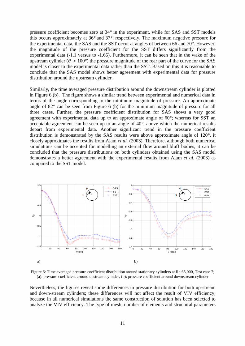
pressure coefficient becomes zero at 34° in the experiment, while for SAS and SST models
this occurs approximately at 36° and 37°, respectively. The maximum negative pressure for
the experimental data, the SAS and the SST occur at angles of between 66 and 70°. However,
the magnitude of the pressure coefficient for the SST differs significantly from the
experimental data (-1.1 versus to -1.65). Furthermore, it can be seen that in the wake of the
upstream cylinder (𝜃 > 100°) the pressure magnitude of the rear part of the curve for the SAS
model is closer to the experimental data rather than the SST. Based on this it is reasonable to
conclude that the SAS model shows better agreement with experimental data for pressure
distribution around the upstream cylinder.
Similarly, the time averaged pressure distribution around the downstream cylinder is plotted
in Figure 6 (b). The figure shows a similar trend between experimental and numerical data in
terms of the angle corresponding to the minimum magnitude of pressure. An approximate
angle of 82° can be seen from Figure 6 (b) for the minimum magnitude of pressure for all
three cases. Further, the pressure coefficient distribution for SAS shows a very good
agreement with experimental data up to an approximate angle of 60°; whereas for SST an
acceptable agreement can be seen up to an angle of 40°, above which the numerical results
depart from experimental data. Another significant trend in the pressure coefficient
distribution is demonstrated by the SAS results were above approximate angle of 120°, it
closely approximates the results from Alam et al. (2003). Therefore, although both numerical
simulations can be accepted for modelling an external flow around bluff bodies, it can be
concluded that the pressure distributions on both cylinders obtained using the SAS model
demonstrates a better agreement with the experimental results from Alam et al. (2003) as
compared to the SST model.
a) b)
Figure 6: Time averaged pressure coefficient distribution around stationary cylinders at Re 65,000, Test case 7;
(a): pressure coefficient around upstream cylinder, (b): pressure coefficient around downstream cylinder
Nevertheless, the figures reveal some differences in pressure distribution for both up-stream
and down-stream cylinders; these differences will not affect the result of VIV efficiency,
because in all numerical simulations the same construction of solution has been selected to
analyze the VIV efficiency. The type of mesh, number of elements and structural parameters
0 20 40 60 80 100 120 140 160 180-1.5
-1
-0.5
0
0.5
1
1.5
(deg.)
CP
SAS
SST
EXP
0 20 40 60 80 100 120 140 160 180-1.4
-1.2
-1
-0.8
-0.6
-0.4
-0.2
0
(deg.)
CP
SAS
SST
EXP

12
were kept constant through the analysis. In addition, in order to ensure the accuracy of the
findings, mean drag and lift coefficients of each turbulence model for both upstream and
downstream cylinders, as well as Strouhal numbers, have been also compared with the data
reported by Alam et al. (2003). The time history of the drag coefficients have been plotted for
both the SAS and SST models in Figures 7 and 8, from which the mean drag coefficients of
the cylinders have been calculated. The findings have been summarised in Table 3. The table
compares the numerical results with experimental data and quantifies differences between
each parameter. Differences between values in mean drag coefficients and Strouhal number
associated with both models are in an acceptable range (less than 10% difference) revealing
that all numerical findings sufficiently agree with the experimental data, however, the error of
the mean drag coefficient of the upstream cylinder in SAS model is larger compared to the
SST model. One of the most significant parameters which can directly affect the efficiency of
the VIV power is the frequency of vortices and consequently the Strouhal number (Equation
13). Fortunately, the discrepancy of the numerical findings and experimental value is
acceptable to both models, particularly in SAS model.
Figure 7: Time history of the drag coefficients of the upstream (top) and downstream (bottom) cylinders
obtained with SST model, Test case 7
Figure 8: Time history of the drag coefficients of the upstream (top) and downstream (bottom) cylinders
obtained with SAS model, Test case 7
0 1 2 3 4 5 6 7 8 9 100
0.5
1
1.5
2
Flow Time (s)
CD
,up
CD history (SST model)
0 1 2 3 4 5 6 7 8 9 10-0.5
0
0.5
1
1.5
Flow Time (s)
CD
,do
wn
0 2 4 6 8 10 12-1
0
1
2
Flow Time (s)
CD
,up
CD history (SAS model)
0 2 4 6 8 10 12-1
0
1
2
Flow Time (s)
CD
,do
wn

13
Table 3: Comparison of mean drag coefficients and Strouhal number with experiment data at Re 65,000 for
x/D=4.5
Lift coefficients of upstream and downstream cylinders
The time history of lift coefficients of upstream and downstream cylinders have been plotted for the
SAS and SST models (Figure 9 and 10). Figure 9 shows that the magnitude of lift coefficients in SST
model are approximately 0.35 and 0.53 for upstream and downstream cylinders, respectively. The lift
coefficients of cylinders obtained with SAS model show higher values which are equal to 0.5 and 0.75
in that order (Figure 9). This means that both models demonstrate approximately 50% increase in lift
coefficient of the downstream cylinder, which confirms the findings of previous researchers
(Zdravkovich and Pridden 1977, Alam et al. 2003). Alam et al. (2003) who showed that at x=4.5D the
lift coefficient for upstream and downstream cylinders are 0.46 and 0.73, respectively (see Figure 10
for downstream cylinder). The comparison between numerical findings and experimental data reveals
that there is an appropriate agreement (less than 10% differences) between SAS results and
experimental recorded data.
Figure 9: Time history of the lift coefficients of the upstream (top) and downstream (bottom) cylinders obtained
with SST model
0 1 2 3 4 5 6 7 8 9 10-1
-0.5
0
0.5
1
Flow Time (s)
CL
,Up
CL history (SST model)
0 1 2 3 4 5 6 7 8 9 10-1
-0.5
0
0.5
1
Flow Time (s)
CL
,do
wn
𝐶𝐷 𝑢𝑝 Difference
between Num.
and Exp.
𝐶𝐷 𝑑𝑜𝑤𝑛 Difference
between Num.
and Exp.
St Difference
between Num.
and Exp.
SST 1.35 3.8% 0.29 6.4% 0.192 4.0%
SAS 1.36 4.6% 0.32 3.2% 0.205 2.5%
Exp. data 1.30 ---- 0.31 ---- 0.2 ----

14
Figure 10: Time history of the lift coefficients of the upstream (top) and downstream (bottom) cylinders
obtained with SAS model
The lift coefficient of downstream cylinder has major impact on the efficiency of the VIV
power. A comparison of the calculated lift coefficient with the Alam et al. (2003)
experimental data are shown on Figure 11. It is clear that the lift coefficient of the stationary
downstream cylinder can be affected by increasing the spacing between cylinders. Also clear
is the trend is similar between the two data sets albeit with some discrepancy in the absolute
values.
Based on the data presented above the SAS model was used for the rest of Test cases
presented in this paper.
Figure11: Variation in the lift coefficient of stationary downstream cylinders as a function of spacing ratio
0 2 4 6 8 10 12-1
-0.5
0
0.5
1
Flow Time (s)C
L,U
p
CL history (SAS model)
0 2 4 6 8 10 12-1
-0.5
0
0.5
1
Flow Time (s)
CL
,do
wn
1 1.5 2 2.5 3 3.5 4 4.5 50
0.2
0.4
0.6
0.8
1
1.2
x/D
CL
Alam et al. 2003-downstream cyl.
Numerical results (SAS)-downstream cyl.
Alam et al. 2003-upstream cyl.
Numerical results (SAS)-upstream cyl.

15
Power efficiency of VIV for different arrangements of cylinders
The thirty five cylinder arrangements detailed in Table 1 have been modelled in this study.
The aim was to investigate the efficiency of VIV power that can be extracted from a
downstream cylinder at a Reynolds number 65,000. For all simulations the mass and damping
ratios were kept constant and equal to 𝑚∗ =2.6 and 𝜁 = 0.007, respectively (based on
experimental data of Assi 2009). The response of the downstream elastically mounted
cylinder at different positions has been interpreted by ANSYS Fluent based on the equation
of motion which was defined in a UDF file. Figure 12 reveals a typical behavior of the
elastically mounted cylinder at x=4D, y= 1D (Test case 20). The figure shows that the peak
magnitude of lift coefficient of downstream cylinder is approximately 1.9.
Figure 12: VIV responses of downstream cylinder for Test case 20 (x/D = 4, y/D = 1)
Furthermore, in order to compare the results with the experimental data of Assi (2009) a
simulation was conducted at Re=30,000. The arrangement of cylinders in this simulation
follows the Test case 6 (see Table 1). Comparing the magnitude displacement of the
downstream cylinder with experiments of Assi (2009) shows that there is a good agreement
between numerical findings and experimental data. The values obtained for the displacement
and lift coefficient in the experiments of Assi (2009), for the same reduced velocity (𝑉𝑟 =𝑈 𝑓. 𝐷) , are 0.7D and 1.5, respectively (Figure 13).
5 5.5 6 6.5 7 7.5 8 8.5 9 9.5
-2
0
2
CL
,do
wn
5 5.5 6 6.5 7 7.5 8 8.5 9 9.5
-100
0
100
FL,d
ow
n (
N)
5 5.5 6 6.5 7 7.5 8 8.5 9 9.5-2
0
2
_ y(m
/s)
5 5.5 6 6.5 7 7.5 8 8.5 9 9.5
-1
0
1
y/D
Flow Time (s)

16
Figure 13: VIV response of the downstream cylinder in Test case 6 (x/D = 4, y/D = 0) and Re=30,000.
The efficiency of VIV can be calculated using Equation (13), which considers the phase
angle between the force and displacement and use the responses of the elastic mounted
cylinder (Figure 12). For instance in Test case 1 the efficiency of VIV is;
𝜂𝑉𝐼𝑉 =
1.21 × 5.1 × (0.4 × 0.05) × 1
1.306= 9.4%
Similarly, the efficiency of VIV power for other cases can be calculated considering the lift
coefficient, the magnitude and relative phase of the displacement of the downstream cylinder
in each simulation. It should be noted that the average of the magnitude of lift coefficient has
been chosen to calculate the efficiency of the VIV power.
The numerical results including Strouhal number, the peak frequency of lift coefficient, the
average magnitude of the lift coefficient, the non-dimensional amplitude 𝑦/D, and finally the
efficiency of VIV power are summarized in Table 4. They demonstrate that the efficiency of
VIV power can be varied by changing the location of downstream cylinder. For the cases
investigated, the table shows five groups of data which have been categorized based on y/D
and it can be argued that, the best location to capture VIV energy is related to group four
according to the obtainable efficiencies. Furthermore, based on the findings, it is clear that
VIV efficiency is weakly dependent on the frequency of the vortices and strongly dependent
on the lift coefficient and the displacement of downstream cylinder.
To find the optimum zone to capture the VIV power among the cases investigated, isolines
contours of VIV efficiency has been plotted in Figure 14. From Figure 14 it is shown that for
the simulated cases, the VIV efficiency varies based on the location of the downstream
cylinder and the maximum obtainable efficiency of VIV power is 48.4%. The results
illustrate that among the five simulated groups of constant 𝑦/D the fourth group of 𝑦/D=1.5
gives the maximum accessible values of VIV efficiency. Among those an efficiency of 48.4%
was obtained for x/D=4 which is comparable to that of the turbine system which according to
Betz limit is 59.3%. These results should encourage researchers to further develop the VIV
concept to optimize this method for the production of hydropower energy. An extensive
9.5 10 10.5 11 11.5 12 12.5 13-2
-1
0
1
2
CL
,do
wn
9.5 10 10.5 11 11.5 12 12.5 13-1
-0.5
0
0.5
1
y/D
Flow Time (s)

17
experimental study is about to commence in order to demonstrate the relative change in VIV
efficiency for the above configurations and to determine the maximum actual efficiency
achievable.
Table 4: Results of the 35 Test cases including Strouhal number, Shedding frequency, lift coefficient,
non-dimensional displacement and VIV efficiency
Groups Test case 𝑥/D 𝑦/D Strouhal f (Hz) 𝑪𝑳 𝒚𝒎𝒂𝒙/D 𝜼𝑽𝑰𝑽
(%)
1 1.5 0 0.195 5.1 1.21 0.40 9.4
2 2 0 0.165 4.3 0.81 0.60 8.0
3 2.5 0 0.171 4.46 0.75 0.90 11.5
1 4 3 0 0.187 4.88 1.07 0.65 13.1
5 3.5 0 0.191 4.98 1.10 0.90 18.8
6 4 0 0.170 4.44 1.82 0.92 28.5
7 4.5 0 0.164 4.28 1.76 0.82 23.7
8 1.5 0.5 0.172 4.49 0.8 0.70 9.6
9 2 0.5 0.183 4.77 0.55 0.70 7.03
10 2.5 0.5 0.185 4.83 0.85 0.90 14.1
2 11 3 0.5 0.183 4.77 0.98 0.94 16.8
12 3.5 0.5 0.202 5.27 1.35 0.90 24.5
13 4 0.5 0.204 5.32 1.40 0.85 24.2
14 4.5 0.5 0.214 5.58 1.70 0.70 25.4
15 1.5 1 0.197 5.14 1.60 0.85 26.8
16 2 1 0.168 4.38 2.05 0.60 20.7
17 2.5 1 0.216 5.64 2.40 0.70 36.2
3 18 3 1 0.176 4.60 2.40 0.81 34.2
19 3.5 1 0.200 5.22 2.00 0.90 35.9
20 4 1 0.168 4.38 1.90 0.97 31.0
21 4.5 1 0.214 5.58 2.00 0.80 34.1
22 1.5 1.5 0.233 6.08 2.00 0.40 18.6
23 2 1.5 0.220 5.74 2.80 0.60 36.9
24 2.5 1.5 0.202 5.27 2.50 0.90 45.3
4 25 3 1.5 0.220 5.74 2.10 0.90 41.5
26 3.5 1.5 0.198 5.17 2.00 0.90 35.6
27 4 1.5 0.233 6.08 2.60 0.80 48.4
28 4.5 1.5 0.233 6.08 2.60 0.65 39.3
29 1.5 2 0.189 4.93 2.10 0.50 19.9
30 2 2 0.183 4.77 2.30 1.00 42.2
31 2.5 2 0.222 5.79 2.85 0.70 44.2
5 32 3 2 0.183 4.77 1.08 0.85 16.8
33 3.5 2 0.225 5.87 2.50 0.80 44.9
34 4 2 0.222 5.79 2.10 0.72 33.5
35 4.5 2 0.220 5.74 2.30 0.70 35.3

18
Figure 14: Isolines contours of calculated VIV efficiency percentages as a function of the location of the
downstream cylinder
Conclusions
Vortex Induced Vibration in the wake of a single cylinder is a relatively new concept for the
production of hydropower energy from oceans and shallow rivers. The availability of ocean
current flow and shallow rivers in the world, even at low speeds, provide an opportunity for a
new viable method for hydropower generation.
The arrangement of bluff bodies is one outstanding feature which can significantly affect
VIV. In this study, two numerical models were utilized and compared to investigate the
external turbulent flow around two circular cylinders with different configurations. In these
arrangements the upstream cylinder was stationary while the downstream one was supported
by an elastic structure. SST and SAS turbulence models have been compared by investigating
the flow behavior around cylinders. The Reynolds number has been chosen based on the
previous experiments of Alam et al. (2003) and Assi (2009) to validate the numerical data
while both cylinders are stationary. Validation of numerical study was conducted by
comparison of the pressure coefficients of cylinders with available experimental values.
Additionally, to ensure the accuracy of simulation other parameters such as drag and lift
coefficients and Strouhal number obtained from the numerical models were also compared
with the recorded experimental data. Both turbulence models were observed to show a good
agreement with the experimental findings. However, in comparison with the SST model, the
lift coefficients for both cylinders, calculated using the SAS model, were in excellent
agreement with the experimental data.
1.5 2 2.5 3 3.5 4 4.5-2
-1.5
-1
-0.5
0
0.5
1
1.5
2
10
10
20
20
20
20
20
20
20
3030
30
30
3030
30
30
30
30
40
40
40
40
40
40
40
40
x/D
y/D

19
For the cylinder with an elastic support, the responses of downstream cylinder were
determined using the SAS model. The response of the downstream cylinder demonstrates that
the location of the cylinder can significantly affect the efficiency of VIV power. Maximum
efficiency of 48.4% was obtained in the current study when the downstream cylinder was
located at 𝑥=4D, 𝑦=1.5D in respect to the upstream cylinder.
The numerically calculated values of efficiency reveal that it is very sensitive to the
geometric arrangement. Furthermore, it was shown that the lift coefficient and displacement
of downstream cylinder are more significant parameters than the vortex shedding frequency
in influencing the efficiency of VIV power.
References
Alam, M.M., Moriya, M., Takai, K. & Sakamoto, H., 2003. Fluctuating fluid forces acting on
two circular cylinders in a tandem arrangement at a subcritical Reynolds number.
Journal of Wind Engineering and Industrial Aerodynamics, 91 (1), 139-154.
Alam, M.M. & Zhou, Y., 2003. Dependence of Strouhal number, drag and lift on the ratio of
cylinder diameters in a two-tandem cylinder. 750-757.
Anagnostopoulos, P. & Bearman, P., 1992. Response characteristics of a vortex-excited
cylinder at low Reynolds numbers. Journal of Fluids and Structures, 6 (1), 39-50.
Assi, G., 2009. Mechanisms for flow-induced vibration of interfering bluff bodies. PhD
thesis, Imperial College London, London, UK.
Bearman, P.W., 1984. Vortex shedding from oscillating bluff bodies. Fluid Mechanics, 16,
195-222.
Bernitsas, M. & Raghavan, K., 2004. Converter of current/tide/wave energy. Provisional
Patent Application. United States Patent and Trademark Office Serial
NO.60/628,252.
Bernitsas, M.M., Ben-Simon, Y., Raghavan, K. & Garcia, E., 2009. The VIVACE converter:
Model tests at high damping and Reynolds number around 10. Journal of Offshore
Mechanics and Arctic Engineering, 131, 1-12.
Bernitsas, M.M., Raghavan, K., Ben-Simon, Y. & Garcia, E., 2008. VIVACE (vortex
induced vibration aquatic clean energy): A new concept in generation of clean and
renewable energy from fluid flow. Journal of Offshore Mechanics and Arctic
Engineering, 130, 1-15.
Blevins, R.D., 1990. Flow-induced vibration. Krieger publishing company, Malabar,
Florida, USA.
Carmo, B.S., 2005. Estudo numerico do escoamento ao redor de cilindros alinhados. Master's
thesis, University of Sao Paulo, Brazil.

20
Chang, C.C.J., Ajith Kumar, R. & Bernitsas, M.M., 2011. VIV and galloping of single
circular cylinder with surface roughness at 3.0× 10⁴ ≪ Re ≪1.2× 10
5. Ocean
Engineering. Volume 38, 1713–1732.
Cheng, Y., Lien, F., Yee, E. & Sinclair, R., 2003. A comparison of large eddy simulations
with a standard k-w Reynolds-averaged Navier–Stokes model for the prediction of a
fully developed turbulent flow over a matrix of cubes. Journal of Wind Engineering
and Industrial Aerodynamics, 91 (11), 1301-1328.
Didier, E., 2007. Simulation de l'écoulement autour de deux cylindres en tandem. Comptes
Rendus Mecanique, 335 (11), 696-701.
Egorov, Y., Menter, F., Lechner, R. & Cokljat, D., 2010. The scale-adaptive simulation
method for unsteady turbulent flow predictions. Part 2: Application to complex flows.
Flow, Turbulence and Combustion, 85 (1), 139-165.
Govardhan, R. & Williamson, C., 2000. Modes of vortex formation and frequency response
of a freely vibrating cylinder. Journal of Fluid Mechanics, 420, 85-130.
Güney, M. & Kaygusuz, K., 2010. Hydrokinetic energy conversion systems: A technology
status review. Renewable and Sustainable Energy Reviews, 14 (9), 2996-3004.
Huera-Huarte, F.J. & Bearman, P.W., 2009. Wake structures and vortex-induced vibrations
of a long flexible cylinder—part 2: Drag coefficients and vortex modes. Journal of
Fluids and Structures, 25 (6), 991-1006.
Igarashi, T., 1981. Characteristics of the flow around two circular cylinders arranged in
tandem. I. JSME International Journal Series B, 24, 323-331.
Jauvtis, N. & Williamson, C.H.K., 2003. Vortex-induced vibration of a cylinder with two
degrees of freedom. Journal of Fluids and Structures, 17 (7), 1035-1042.
Khan, M., Bhuyan, G., Iqbal, M. & Quaicoe, J., 2009. Hydrokinetic energy conversion
systems and assessment of horizontal and vertical axis turbines for river and tidal
applications: A technology status review. Applied Energy, 86 (10), 1823-1835.
Kitagawa, T. & Ohta, H., 2008. Numerical investigation on flow around circular cylinders in
tandem arrangement at a subcritical reynolds number. Journal of Fluids and
Structures, 24 (5), 680-699.
Kuo, C., Chein, S. & Hsieh, H., 2008. Self-sustained oscillations between two tandem
cylinders at Reynolds number 1,000. Experiments in Fluids, 44 (4), 503-517.
Langtry, R.B. & Menter, F.R., 2009. Correlation-based transition modeling for unstructured
parallelized computational fluid dynamics codes. AIAA journal, 47 (12), 2894-2906.
Lee, J.H., Xiros, N. & Bernitsas, M.M., 2011. Virtual damper–spring system for VIV
experiments and hydrokinetic energy conversion. Ocean Engineering, 38 (5-6), 732-
747.

21
Liaw, K., 2005. Simulation of flow around bluff bodies and bridge deck sections using CFD.
Thesis submitted to the University of Nottingham for the degree of Doctor of Philosophy.
Ljungkrona, L., Norberg, C. & Sunden, B., 1991. Free-stream turbulence and tube spacing
effects on surface pressure fluctuations for two tubes in an in-line arrangement.
Journal of Fluids and Structures, 5 (6), 701-727.
Menter, F. & Egorov, Y., 2005. A scale-adaptive simulation model using two-equation
modelsed. American Institute of Aeronautics and Astronautics, 1-13.
Menter, F. & Egorov, Y., 2010. The scale-adaptive simulation method for unsteady turbulent
flow predictions. Part 1: Theory and model description. Flow, Turbulence and
Combustion, 85 (1), 113-138.
Menter, F., Garbaruk, A., Smirnov, P., Cokljat, D. & Mathey, F., 2010. Scale-adaptive
simulation with artificial forcing. Progress in Hybrid RANS-LES Modelling, 235-246.
Menter, F.R., 1994. Two-equation eddy-viscosity turbulence models for engineering
applications. AIAA journal, 32 (8), 1598-1605.
Palau-Salvador, G., Stoesser, T. & Rodi, W., 2008. LES of the flow around two cylinders in
tandem. Journal of Fluids and Structures, 24 (8), 1304-1312.
Raghavan, K. & Bernitsas, M., 2011. Experimental investigation of Reynolds number effect
on vortex induced vibration of rigid circular cylinder on elastic supports. Ocean
Engineering, 38 (5), 719-731.
Sagaut, P., 2001. Large eddy simulation for incompressible flows: Springer Berlin.
Vries, O., 1983. On the theory of the horizontal-axis wind turbine. Annual Review of Fluid
Mechanics, 15 (1), 77-96.
Williamson, C. & Govardhan, R., 2004. Vortex-induced vibrations. Annual Review of Fluid
Mechanics.,36, 413-455.
Williamson, C. & Roshko, A., 1988. Vortex formation in the wake of an oscillating cylinder.
Journal of Fluids and Structures, 2 (4), 355-381.
Zdravkovich, M., 1987. The effects of interference between circular cylinders in cross flow.
Journal of Fluids and Structures, 1 (2), 239-261.
Zdravkovich, M. & Pridden, D., 1977. Interference between two circular cylinders; series of
unexpected discontinuities. Journal of Wind Engineering and Industrial
Aerodynamics, 2 (3), 255-270.


![Control of flow around a circular cylinder using a ... · the circular cylinder [1, 2]. Figure 1: Drag coefficient of rough and smooth circular cylinders. It is also known that the](https://img.dokumen.tips/doc/110x75/5e9700258a215e1f8f73e60f/control-of-flow-around-a-circular-cylinder-using-a-the-circular-cylinder-1.jpg)


