The Econometrics of the Simple Regression Modelpersonal.strath.ac.uk/gary.koop/ec311/Topic_3_slides... · 2014-10-09 · The Econometrics of the Simple Regression Model Multiple regression

The Econometrics of the Simple Regression Model

() Introductory Econometrics: Topic 3 1 / 34

The Econometrics of the Simple Regression Model

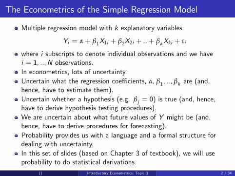
Multiple regression model with k explanatory variables:

Yi = α+ β1X1i + β2X2i + ..+ βkXki + εi

where i subscripts to denote individual observations and we havei = 1, ..,N observations.In econometrics, lots of uncertainty.Uncertain what the regression coeffi cients, α, β1, .., βk are (and,hence, have to estimate them).Uncertain whether a hypothesis (e.g. βj = 0) is true (and, hence,have to derive hypothesis testing procedures).We are uncertain about what future values of Y might be (and,hence, have to derive procedures for forecasting).Probability provides us with a language and a formal structure fordealing with uncertainty.In this set of slides (based on Chapter 3 of textbook), we will useprobability to do statistical derivations.


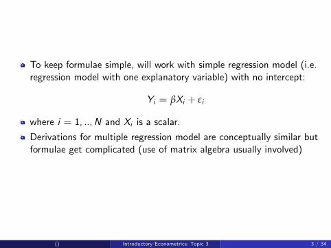
To keep formulae simple, will work with simple regression model (i.e.regression model with one explanatory variable) with no intercept:

Yi = βXi + εi

where i = 1, ..,N and Xi is a scalar.

Derivations for multiple regression model are conceptually similar butformulae get complicated (use of matrix algebra usually involved)


The Classical Assumptions for the Regression Model

Now let us return to the regression model.

We need to make some assumptions to do any statistical derivationsand start with the classical assumptions

1 E (Yi ) = βXi .2 var (Yi ) = σ2.3 cov (Yi ,Yj ) = 0 for i 6= j .4 Yi is Normally distributed5 Xi is fixed. It is not a random variable.


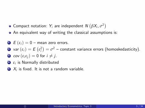
Compact notation: Yi are independent N(

βXi , σ2)

An equivalent way of writing the classical assumptions is:

1 E (εi ) = 0 —mean zero errors.2 var (εi ) = E

(ε2i)= σ2 —constant variance errors (homoskedasticity).

3 cov (εi εj ) = 0 for i 6= j .4 εi is Normally distributed5 Xi is fixed. It is not a random variable.


Motivation for Classical Assumptions

Regression model fits a straight line through an XY-plot.

E (Yi ) = βXi is the linearity assumption.

Second assumption: all observations have the same variance(homoskedasticity).

Ex. where this might not be a good assumption. House price data.Small houses all the same. Big houses more diverse. If so, houseprices might be more diverse for big houses (heteroskedasticity).

Third assumption: observations uncorrelated with one another.

This assumption is usually reasonable with cross-sectional data (e.g.in a survey, response of person1 and person 2 are unrelated).

For time series data not a good assumption (e.g. interest rate nowand last month are correlated with one another)


Fourth assumption (Y is Normal), harder to motivate.

In many empirical applications, Normality is reasonable.

Asymptotic theory can be used to relax this assumption. We will notcover this in this course (but see Appendix C and Appendices at endof several chapters)

Fifth assumption (explanatory variable not a random variable) is goodin experimental sciences, but maybe not in social sciences.

We will talk about relaxing these assumptions in later chapters.


The Ordinary Least Squares (OLS) Estimator

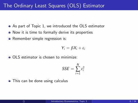
As part of Topic 1, we introduced the OLS estimator

Now it is time to formally derive its properties

Remember simple regression is:

Yi = βXi + εi

OLS estimator is chosen to minimize:

SSE =N

∑i=1

ε2i

This can be done using calculus


Choose β to minimizeN

∑i=1(Yi − βXi )

2

Taking first derivavative with respect to β

dSSEdβ

=N

∑i=12 (Yi − βXi ) (−Xi )

= 2N

∑i=1

(−XiYi + βX 2i

)= 2

N

∑i=1

βX 2i − 2N

∑i=1XiYi

Set first derivative to zero and solve for β gives us the OLS estimator:

β̂ =

N

∑i=1XiYi

N

∑i=1X 2i


Properties of OLS Estimator

First let me derive an alternative way of writing the OLS estimatorwhich we will use several times

Label it equation (*) for future reference

β̂ =∑XiYi

∑X 2i=

∑Xi (Xi β+ εi )

∑X 2i= β+

∑Xi εi

∑X 2i(*)

Property 1: OLS is unbiased under the classical assumptions

E(

β̂)= β

Proof is on the next slide


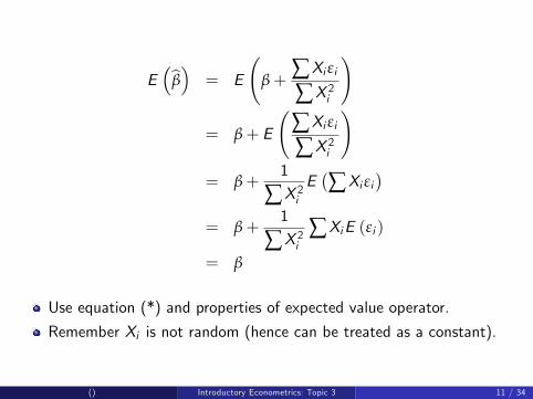
E(

β̂)= E

(β+

∑Xi εi

∑X 2i

)

= β+ E

(∑Xi εi

∑X 2i

)= β+

1

∑X 2iE(∑Xi εi

)= β+

1

∑X 2i∑XiE (εi )

= β

Use equation (*) and properties of expected value operator.

Remember Xi is not random (hence can be treated as a constant).


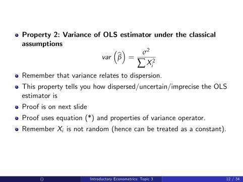
Property 2: Variance of OLS estimator under the classicalassumptions

var(

β̂)=

σ2

∑X 2i

Remember that variance relates to dispersion.

This property tells you how dispersed/uncertain/imprecise the OLSestimator is

Proof is on next slide

Proof uses equation (*) and properties of variance operator.

Remember Xi is not random (hence can be treated as a constant).


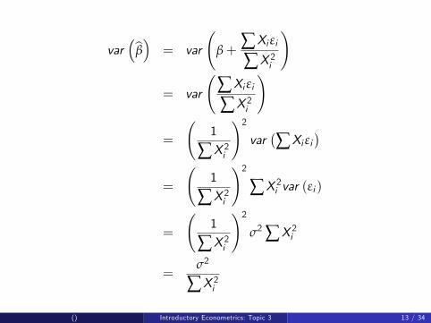
var(

β̂)= var

(β+

∑Xi εi

∑X 2i

)

= var

(∑Xi εi

∑X 2i

)

=

(1

∑X 2i

)2var(∑Xi εi

)=

(1

∑X 2i

)2∑X 2i var (εi )

=

(1

∑X 2i

)2σ2 ∑X 2i

=σ2

∑X 2i


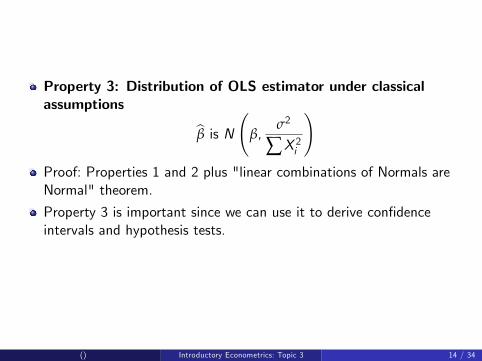
Property 3: Distribution of OLS estimator under classicalassumptions

β̂ is N

(β,

σ2

∑X 2i

)Proof: Properties 1 and 2 plus "linear combinations of Normals areNormal" theorem.

Property 3 is important since we can use it to derive confidenceintervals and hypothesis tests.


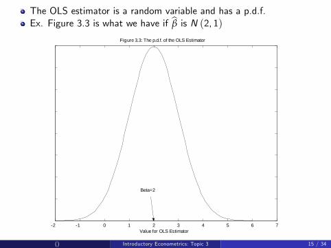
The OLS estimator is a random variable and has a p.d.f.Ex. Figure 3.3 is what we have if β̂ is N (2, 1)

2 1 0 1 2 3 4 5 6 7

Figure 3.3: The p.d.f. of the OLS Estimator

Value for OLS Estimator

Beta=2


Desireable features of any estimator: want it unbiased and want it tohave as small a variance as possible.

An unbiased estimator is said to be effi cient relative to another if ithas a smaller variance.

See Figure 3.4 on next slide for an illustration of how this might lookin practice

See Problem Set 2 for an extended example


6 4 2 0 2 4 6 8 10 12

Figure 3.4: The p.d.f.s of the OLS Estimator and A Less Efficient Estimator

Value for Estimator

P.d.f. of OLS Estimator

P.d.f. of Other Estimator


Property 4: The Gauss-Markov TheoremIf the classical assumptions hold, then OLS is the best, linearunbiased estimator,

where best = minimum variance

linear = linear in y.

Short form: "OLS is BLUE"

I will not give proof here (see pages 84-85 of textbook)

Note: the assumption of Normal errors is NOT required to proveGauss-Markov theorem. Hence, OLS is BLUE even if errors are notNormal.


Property 5: Under the Classical Assumptions, OLS is themaximum likelihood estimatorMaximum likelihood is another statistical principal for choosingestimators.

Textbook has a discussion of this topic, but I do not have time tocover in lectures.


Deriving a Confidence Interval for Beta

Assume σ2 known (discuss relaxing this assumption later).

Use Property 3 to obtain:

Z =β̂− β√

σ2

∑X 2i

is N (0, 1)

Can use statistical tables for the Normal distribution to makeprobability statements.

For instance to get a 95% confident you begin with the followingprobability statement:

Pr [−1.96 ≤ Z ≤ 1.96] = 0.95


Then rearrange the inequalities to put β in the middle:

Pr

−1.96 ≤ β̂− β√σ2

∑X 2i

≤ 1.96

= 0.95Then do some more rearranging of the inequalities:

Pr

[β̂− 1.96

√σ2

∑X 2i≤ β ≤ β̂+ 1.96

√σ2

∑X 2i

]= 0.95


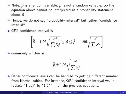
Note: β̂ is a random variable, β is not a random variable. So theequation above cannot be interpreted as a probability statementabout β

Hence, we do not say "probability interval" but rather "confidenceinterval".

95% confidence interval is[β̂− 1.96

√σ2

∑X 2i≤ β ≤ β̂+ 1.96

√σ2

∑X 2i

]

commonly written as:

β̂± 1.96√

σ2

∑X 2i

Other confidence levels can be handled by getting different numberfrom Normal tables. For instance, 90% confidence interval wouldreplace "1.96)" by "1.64" in all the previous equations.


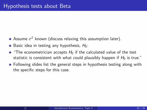
Hypothesis tests about Beta

Assume σ2 known (discuss relaxing this assumption later).

Basic idea in testing any hypothesis, H0:

“The econometrician accepts H0 if the calculated value of the teststatistic is consistent with what could plausibly happen if H0 is true.”

Following slides list the general steps in hypothesis testing along withthe specific steps for this case.


Step1: Specify a hypothesis, H0.

In this case, we will choose H0: β = 0

Step 2: Specify a test statistic

In this case, we can use the Z-score as a test statistic:

Z =β̂− β√

σ2

∑X 2i


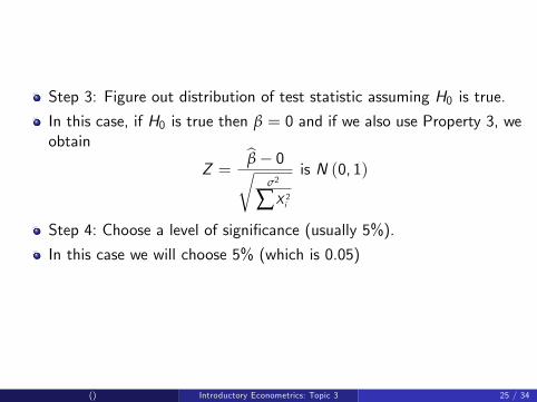
Step 3: Figure out distribution of test statistic assuming H0 is true.

In this case, if H0 is true then β = 0 and if we also use Property 3, weobtain

Z =β̂− 0√

σ2

∑X 2i

is N (0, 1)

Step 4: Choose a level of significance (usually 5%).

In this case we will choose 5% (which is 0.05)


Step 5: Use Steps 3 and 4 to get a critical value.

Critical value = 1.96 (from Normal statistical tables)

Step 6: Calculate your test statistic and compare to critical value.Reject H0 if absolute value of test statistic is greater than criticalvalue (else accept H0).

In this case we reject H0 : β = 0 if |Z | > 1.96.


Modifications when Sigma-squared is unknown

σ2 appears in previous formulae for confidence interval and teststatistic.

What to do when it is unknown?

Replace it by an estimate

This estimate is commonly referred to as s2

Note: we used this notation before as the sample variance of arandom sample Y1, ..,YN (don’t get confused, we are just extendingthis concept to the case of regression)


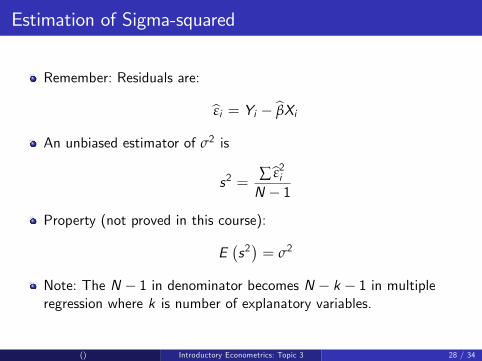
Estimation of Sigma-squared

Remember: Residuals are:

ε̂i = Yi − β̂Xi

An unbiased estimator of σ2 is

s2 =∑ ε̂2iN − 1

Property (not proved in this course):

E(s2)= σ2

Note: The N − 1 in denominator becomes N − k − 1 in multipleregression where k is number of explanatory variables.


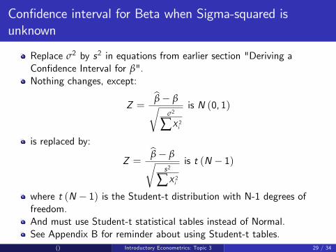
Confidence interval for Beta when Sigma-squared isunknown

Replace σ2 by s2 in equations from earlier section "Deriving aConfidence Interval for β".Nothing changes, except:

Z =β̂− β√

σ2

∑X 2i

is N (0, 1)

is replaced by:

Z =β̂− β√

s2

∑X 2i

is t (N − 1)

where t (N − 1) is the Student-t distribution with N-1 degrees offreedom.And must use Student-t statistical tables instead of Normal.See Appendix B for reminder about using Student-t tables.


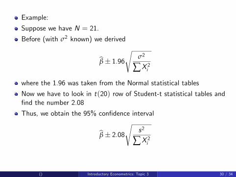
Example:

Suppose we have N = 21.

Before (with σ2 known) we derived

β̂± 1.96√

σ2

∑X 2i

where the 1.96 was taken from the Normal statistical tables

Now we have to look in t(20) row of Student-t statistical tables andfind the number 2.08

Thus, we obtain the 95% confidence interval

β̂± 2.08√

s2

∑X 2i


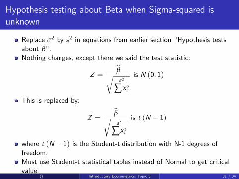
Hypothesis testing about Beta when Sigma-squared isunknown

Replace σ2 by s2 in equations from earlier section "Hypothesis testsabout β".Nothing changes, except there we said the test statistic:

Z =β̂√

σ2

∑X 2i

is N (0, 1)

This is replaced by:

Z =β̂√s2

∑X 2i

is t (N − 1)

where t (N − 1) is the Student-t distribution with N-1 degrees offreedom.Must use Student-t statistical tables instead of Normal to get criticalvalue.


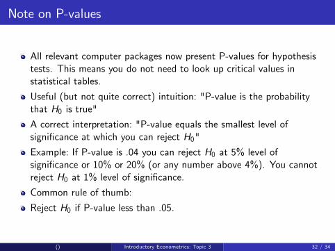
Note on P-values

All relevant computer packages now present P-values for hypothesistests. This means you do not need to look up critical values instatistical tables.

Useful (but not quite correct) intuition: "P-value is the probabilitythat H0 is true"

A correct interpretation: "P-value equals the smallest level ofsignificance at which you can reject H0"

Example: If P-value is .04 you can reject H0 at 5% level ofsignificance or 10% or 20% (or any number above 4%). You cannotreject H0 at 1% level of significance.

Common rule of thumb:

Reject H0 if P-value less than .05.


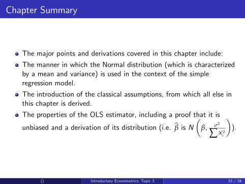
Chapter Summary

The major points and derivations covered in this chapter include:

The manner in which the Normal distribution (which is characterizedby a mean and variance) is used in the context of the simpleregression model.

The introduction of the classical assumptions, from which all else inthis chapter is derived.

The properties of the OLS estimator, including a proof that it is

unbiased and a derivation of its distribution (i.e. β̂ is N(

β, σ2

∑X 2i

)).


The Gauss-Markov theorem which says OLS is BLUE under theclassical assumptions.

The derivation of a confidence interval for β (assuming σ2 is known).

The derivation of a test of the hypothesis that β = 0 (assuming σ2 isknown).

The OLS estimator of σ2.

How the confidence interval and hypothesis test are modified when σ2

is unknown.


Documents

The Econometrics of the Simple Regression Modelpersonal.strath.ac.uk/gary.koop/ec311/Topic_3_slides... · 2014-10-09 · The Econometrics of the Simple Regression Model Multiple regression