The dynamic impact of carbon reduction and renewable support policies on the electricity sector

lable at ScienceDirect

Utilities Policy 28 (2014) 28e41

Contents lists avai

Utilities Policy

journal homepage: www.elsevier .com/locate/ jup

The dynamic impact of carbon reduction and renewable supportpolicies on the electricity sector

Riccardo Fagiani*, Jörn C. Richstein, Rudi Hakvoort, Laurens De VriesFaculty of Technology, Policy and Management, Delft University of Technology, Jaffalaan 5, 2600 GA Delft, The Netherlands

a r t i c l e i n f o

Article history:Received 1 August 2013Received in revised form19 November 2013Accepted 29 November 2013

Keywords:Electricity sectorEU ETSRenewable energy policyDynamic policy interaction

* Corresponding author. Tel.: þ31 655795492.E-mail addresses: [email protected], r

(R. Fagiani).

0957-1787/$ e see front matter � 2013 Elsevier Ltd.http://dx.doi.org/10.1016/j.jup.2013.11.004

a b s t r a c t

Carbon reduction and renewable energy policies are implemented in Europe to improve the sustain-ability of the electricity sector while achieving security of supply. We investigate the interactions be-tween these policies using a dynamic investment model. Our analysis indicates that both policies arenecessary to achieve a sustainable power sector. However, renewable energy generation significantlyaffects carbon markets and could lead to very low prices. These would attract investments in carbonintensive technologies, locking the sector into future higher emissions. To contrast this effect, policymakers may introduce a floor price in the carbon market or adjust the emissions quota periodically.

� 2013 Elsevier Ltd. All rights reserved.

1. Introduction

The European Union set an ambitious target to lower theemissions of greenhouse gases (GHG) and established challenginggoals for the production of energy from renewable energy sources(RES). An Emissions Trading Scheme (ETS) was established at theEuropean level while mechanisms supporting investments in RESare implemented at a national level. A significant sector affected bythese policies is the power industry, since it is one of the primarysectors emitting GHG and many RES technologies are electricitygenerators.

In this paper we investigate the dynamic interactions betweencarbon reduction and renewable energy policies. Both policiesaffect operational and investment decisions concerning renewableand conventional generation in the electricity market. Carbonpolicy adds to the variable cost of conventional generators. Thisaffects their revenue streams and may change the merit order.Renewable energy producers also affect generation dispatch andthus the (future) revenues of the other generators in the market.

While interactions have been studied for equilibrium condi-tions, the dynamic feedback loops between the two policies overtime have been less investigated. Jensen and Skytte (2003) discussthe impact of the correlation between the consumer price and the

[email protected]

All rights reserved.

renewable energy quota on the interactions between carbonreduction and green certificate markets. Linares et al. (2008) pre-sent an oligopolistic partial-equilibrium model simulating theSpanish electricity sector under different energy policy scenarios.Amundsen and Nese (2009) investigate the interaction betweencarbon and renewable energy policies in the Scandinavian regionimplementing an analytical equilibrium model. De Jonghe et al.(2009) use a welfare maximization simulation in order to findequilibrium states for combinations of renewable and carbon policyin a three zone system.

This paper presents a bottom-up investment model whichsimulates the evolution of a hypothetical electricity sector, withcharacteristics close to the Spanish system, under different policyscenarios. This work addresses the following research question: Inwhich manner do CO2 reduction policies and renewable energy sup-port mechanisms dynamically affect each other? This research addsinsights to the analysis of the interactions existing between carbonreduction and renewable energy policy.

We apply a simulation approach that combines elements ofagent-based and system-dynamic modeling. The purpose of ourmodel is to analyze how energy policy instruments affect the in-vestment decisions of generating companies by changing the profitand risk profiles of investment projects (Gross et al., 2010). Weapply the notion of bounded rationality (Simon, 1957), recognizingthat investors are not fully rational when making decisions and donot necessarily optimize but rather satisfice. This means that in-vestors’ decisions may not be optimal, but adequate to comply withtheir expectations. This reflects the fact that investors have

Delta:1_given name

Delta:1_surname

Delta:1_given name

Delta:1_surname

mailto:[email protected]

mailto:[email protected]

http://crossmark.crossref.org/dialog/?doi=10.1016/j.jup.2013.11.004&domain=pdf

www.sciencedirect.com/science/journal/09571787

http://www.elsevier.com/locate/jup

http://dx.doi.org/10.1016/j.jup.2013.11.004



R. Fagiani et al. / Utilities Policy 28 (2014) 28e41 29

informational, intellectual, and computational limitations. Hence,in our model the agents base their investment decisions on avail-able information and on expectations, trying to maximize thetrade-off between risks and profits. Agent behavior is also limitedby their past investment choices, which affect their current gen-eration portfolios, balance sheets and cash positions, reflecting pathdependency. By simulating the impact of carbon reduction andrenewable energy policies on investors’ choices, we model howenergy policy shapes the evolution of the electricity sector(Chappin, 2011).

Our results indicate that while both carbon reduction andrenewable support policies are necessary for improving the sus-tainability of the electricity sector, an aggressive renewable energypolicymay reduce the effectiveness of a carbonmarket in attractinginvestments in carbon-intensive technologies. Renewable elec-tricity generation reduces carbon emissions andmay therefore leadto lower carbon prices; this is part of the reason by the EU ETS iscurrently experiencing a period of low prices (in addition to adecline in energy demand and industrial activity) (Rathmann,2007; Lecuyer and Quirion, 2013). If this causes generation com-panies to invest in coal-fired generators, this may lock the systeminto higher emissions in the future. In the opposite direction, the EUETS does not impose negative side-effects on the national renew-able support mechanisms; rather, a higher CO2 price reduces theneed for RES subsidies.

This paper is organized as follows. Section 2 provides an over-view of policy instruments for supporting renewable energy andreducing carbon emissions, and describes how these are imple-mented in Europe. Section 3 presents the details of the model.Section 4 describes and discuss the results of the simulations.Finally, Section 5 concludes with policy recommendations.

2. Renewable and carbon policy in the European power sector

Carbon reduction and renewable energy policy mechanisms canbe categorized into price-based and quantity-based policies, adistinction made by Weitzman (1974) in a seminal paper on thegeneric case of regulating a particular economic variable. Inquantity-based instruments, the desired level of outcome is set andan artificial market is created in which participants trade certifi-cates to fulfill the policy target. This yields a price for the regulatedvariable. Examples are the emission trading schemes (ETS) for GHG,in which emitters buy emission allowances (and therefore need topay for emissions) and tradable green certificates (TGC) for thepromotion of RES, which are sold by power producers. In price-based policies, on the other hand, the regulator sets a price for aspecific variable, thus, levying a tax on or paying a subsidy to aproducer. Ideally, this is a Pigovian tax, which means it is equal tothe externality cost of the variable. Examples are technology-specific feed-in tariffs for RES technologies and a carbon tax onGHG emissions. Combinations of these policy instruments arepossible as well; however, they represent an increased level ofcomplexity (Hepburn, 2006).

While many publications compare TGC markets with feed-intariffs (FITs), the question of which policy leads to preferable re-sults for society is still debated. Feed-in tariffs have proven to beeffective in reaching policy targets but they suffer from poorer cost-effectiveness (Menanteau et al., 2003). They can be used to stim-ulate technological change, as they can be designed to have atechnological specific component. This can be used to promotetechnologies in their early stages of development, which maypossibly lead to higher dynamic efficiency by inducing technolog-ical learning (Del Rio, 2012). Feed-in tariffs may also limit thewindfall profits that cheaper RES generators experience in a TGCscheme (Haas et al., 2011) (since cheap RES technologies receive the

same remuneration as the marginal technology), and do not causegenerators to charge a risk-premium as they do in a TGCmarket dueto the volatility of the green certificate price. This was investigatedin a precursor to this study which incorporated generator’s riskattitudes and that found that the efficiency of TGC schemes’depended on the risk attitudes towards RES technologies (Fagianiet al., 2013).

The general arguments made by Weitzman (1974) were appliedto carbon policy by Grubb and Newberry (2007). They concludedthat while a well-set, slowly rising carbon tax would probably bemore efficient because it provided more investment certainty(temporal price stability), only a CO2 market in the form of theEuropean ETS was politically viable and credible for such a largearea, due to easier negotiations on quantities than prices andbecause it offered a better promise for global integration. Chappinet al. (2010) presented an agent-based simulation in which theyfound that a carbon tax was more efficient in reducing emissions atsimilar costs to an ETS. Both studies also conclude that setting anappropriate tax is very difficult, due to lack of information. None-theless, Chappin et al. (2010) suggest a relatively low starting tax,with a commitment that it will only be adjusted upwards period-ically, to provide policy flexibility while limiting investoruncertainty.

In the tradition of Tinbergen (1952), the European Unionimplemented different policy instruments for the different policygoals. The establishment of the EU ETS, which was established byDirective 2003/87/EC, has involved three trading phases, from 2005to 2007 (Phase I), 2008e2012 (Phase II), and Phase III since in 2013.The main difference between the phases was in the increasingnumber of sectors that were covered and the allocation of allow-ances, freely or in an auction. While the banking of allowances wasnot allowed between Phase I and Phase II, from Phase II theymay betaken over to Phase III. Renewable energy policy, on the other hand,developed at the initiative of member states. Directive 2009/28/ECimposed legally binding national renewable targets for 2020, whichdiffer between the states and were implemented via NationalRenewable Action Plans (NREAP) (European Commission, 2009;European Commission, 2010). However, no instruction was pro-vided as to the choice of policy instrument for reaching these tar-gets (Haas et al., 2011). In addition, targets for both carbonreduction and renewable energy were established for 2050(European Commission, 2011).

3. Model description

Our model simulates the evolution of a hypothetical powersector with characteristics similar to the Spanish system from 2012to 2050. The model is written and run in Matlab R2011a andcomprehends elements of agent-based and system-dynamicsmethodologies. A previous version of the model was used to eval-uate renewable energy support mechanisms, confronting price-based and quantity-based mechanisms under different risk-aversion investors’ behavior (Fagiani et al., 2013). That analysisdid not consider the interaction between carbon and renewablepolicies; instead, an increasing pigovian tax on carbon emissionwas defined as an exogenous variable. Also, the green certificatemarket was modeled assuming a steady state equilibrium with itsprice reflecting the difference between the average total generationcost of the marginal renewable plant in the market and the averageelectricity price.

For the purpose of this analysis, we added to the model a carbonmarket which covers the power sector exclusively, introducing thecarbon price as an endogenous variable. The green certificate andcarbon prices aremodeled to reflect both short-term and long-termexpectations of the generation companies in order to better reflect

Fig. 1. Flow scheme of the simulation.

R. Fagiani et al. / Utilities Policy 28 (2014) 28e4130

price volatility, and includes the possibility of banking excess greencertificates to comply with future quota obligations.

Similarly to the previous model, the simulation flow consists ofthree main blocks which are repeated every simulated year aspresented in Fig. 1:

� A market block in which the model clears the electricity, thecarbon, and the green certificate markets;

� A forecasting block in which the model centrally estimatesfuture prices for each of these markets;

� An investment block in which the different generating com-panies make decisions about investments and dismantlingexisting power plants.

Three renewable energy and three carbon policy options areimplemented, resulting in a total of nine model runs for eachsimulated scenario. The simulation includes these renewable sup-port mechanisms:

� No RES policy;� A technology specific feed-in tariff system (price-based);� A technology neutral green certificate market (quantity-based).

And the following carbon policy options:

� No CO2 policy;� An increasing tax imposed on CO2 emissions (price-based);� An emissions allowances scheme limiting the discharge of CO2(quantity-based).

We continue by describing in Sections 3.1, 3.2, and 3.3 respec-tively how themodel clears the electricity, the green certificate, andcarbon markets.

3.1. The electricity market

Some measures needed to be taken reduce the computationalcomplexity of the model and the time required to run simulations.The annual load duration curve is approximated with 365 steps,each one including 24 h with similar electricity demand. Electricitydemand is assumed to grow at a constant 1.5% annual rate until2020 and increases to 1.9% afterward. The installed generation ca-pacity at the beginning of the simulation period corresponds to thegeneration mix of Spain in 2012 as presented in Table 1.

We assume that the electricity companies have no market po-wer, thus generators’ bids reflect their marginal costs (includingtheir cost of carbon). For each section of the load-duration curve,the market is cleared by intersecting the supply curve with de-mand, which is assumed to be inelastic. For the sake of simplicity,the model disregards ramping constraints of thermal generatorsand the possible congestion of transmission lines. Nonetheless, toaccount for spike prices during peak load hours, we introduced aconstraint which prevents electricity companies to cover the twodemand sections with the highest loads by starting up power plantswhich have long start-up times. As a consequence, only gas tur-bines and generators that are already dispatched are allowed to bidin the two peak load periods.

Every year, the model updates fuel prices. To reflect the per-formance decrease of old power plants, the model increases thefixed O& cost of generators by 1% every year after the end of theirexpected service life. Technological development is simulated byupdating the characteristics of available technologies annually ac-cording to an exogenous learning curve, which we assume to beindependent from the simulation.

3.2. Renewable energy support mechanisms

In this section we explain how the model simulates feed-intariffs and tradeable green certificates. In both cases the modelends the renewable energy support mechanism in 2050 or if a long-term capacity target is reached. This long-term renewable objectiveis an input variable of the simulation; it corresponds to the finalquota of the green certificate market. For the base scenario a valueof 65% is used. This constraint can be interpreted as a technical limitto the integration of intermittent generators or as a limit imposedby policy makers to limit the cost of subsidizing RES. This is espe-cially necessary in case of a feed-in mechanism without a quantitylimit.

Under a feed-in tariff system, generators are guaranteed a fixedelectricity price during their expected life time, bidding at a nullprice in the electricity market (this distinction is important for REStechnologies with marginal costs greater than zero, i.e., biomasspower plants). After reaching the end of their expected service livesor if no support is given to renewable energy, RES generatorsbehave like conventional generators bidding at marginal cost andreceiving the electricity price until they are dismantled.

We assume the feed-in tariff mechanism to be an open-budgetscheme, so there is no limit for new generators to apply for sub-sidy until the long-term renewable target is reached. This reflectsthe current policy implementation in several European countries.Tariffs are technology-specific and reflect the regulator’s estimateof the average generating cost of each technology. The regulator hasa biased knowledge of generation costs. Tariffs for new technolo-gies are calculated by multiplying the exact generation cost with abiasing factor as indicated in Equation (1), where FDTjt indicates thefeed in tariff level for technology j at year t,Costjt the averagegenerating cost of a plant built in year t with technology j, and BFthe biasing factor which is an input parameter of the model andremains constant during the simulated period.

FDTjt ¼ Costjt � BF (1)

The tariff level has a strong impact on the effectiveness of themechanism. If tariffs are set too low, investors are unlikely to adoptRES technologies and the mechanism is ineffective. High tariffs areeffective but may result in unneccessarily high subsidy costs tosociety. Before running the simulation, we performed a sensitivityanalysis to find a moderate biasing factor which would stimulateinvestments in RES without leading to an excessive subsidy cost.Fig. 2 indicates that there is a notable shift in renewable energyproduction between a biasing factor of 7.5% and 10%, as manyrenewable technologies become competitive with conventionalgenerators in that range. A further increase from 10% to 30% onlyattracts slightly more investment. Therefore, we choose a biasingfactor of 15% for our base case scenario, as it represents a goodcompromise between policy effectiveness and cost-efficiency.

Under a green certificate policy, renewable energy generatorsreceive a green certificate for each MWh of electricity produced

Table 1Installed capacity in Spain in year 2010 (Red Electrica de Espana, 2012).1

Hydro Nuclear Coal Fuel/Gas Combined cycle Wind on-shore Small hydro Biomass PV Other

GW 17.564 7.777 12.210 4.376 27.123 21.239 2.041 0.859 4.249 8.450% 16.6% 7.3% 11.5% 4.1% 25.6% 20.1% 1.9% 0.8% 4.0% 8.0%

Table 2Policy combinations simulated for each scenario run.


during the expected service period, independently of the technol-ogy used. The corresponding electricity that is generated is offeredin the market at a zero price, so the volume of green certificatealways reflects actual renewable electricity production. Existinghydro generators are treated the same way. In order to be compa-rable with the feed-in tariff mechanism in which only new gener-ators are subsidized for a period equivalent to their expected lifetime, renewable energy plants that have reached their expected lifetimes do not receive green certificates and are treated like con-ventional plants.1

The green certificate and the electricity markets are simulatedtogether. In order to obtain an approximation of the electricityprice, the electricity market is cleared first, assuming a null greencertificate price. The renewable energy generators use this elec-tricity price to compute their bids for the green certificate market(as explained further below). After the green certificate market iscleared, renewable energy generators bid their marginal generationcost minus the green certificate price and the electricity market iscleared again. This process is not iterated again since the impact ofthe certificate price on the electricity price is negligible.

Regarding the bidding behavior in the green certificate market,if certificates were not bankable, renewable energy generatorswould bid the difference between the marginal generation cost(CostMt ) and the electricity price (Et), as indicated in (2).

Ct ¼ CostMt � Et (2)

This would result in many generators offering green certificatesat zero price in the market due to zero marginal generation cost ofwind and PV generators. As a consequence, the certificate pricewould fluctuate between zero and the marginal cost of biomass-fueled generators, depending on the supply and demand of greencertificates. Instead, we assume the validity of green certificates tobe unlimited. Market participants are allowed to bank their cer-tificates and use them to comply with future quota obligations. Inthis case, producers are not forced to sell their certificates in themarket during periods of over-supply when the price would beclose to zero.2 Certificate banking thus guarantees a certain bar-gaining power to producers, who could try to offer green certifi-cates at a price higher than their marginal cost in the market in anattempt to raise green certificate prices. In the long run, however, inthe absence of barriers to entry, the threat of new entrants wouldcause the green certificate price to converge towards the differencebetween the average costs of renewable generators and the elec-tricity price, as indicated in Equation (3).

CLT ¼ CostMLT � ELT (3)

Here CLT indicates the long-term certificate price, CostMLT thelong-term average generation cost of the marginal technology andELT the long-term average electricity price.

1 Others include solar thermodynamic and other non-renewable energy sourcesfinanced under the Régimen Especial.

2 This is true for big generating companies that do not urgently require cash forrunning their businesses. Small players could require to sell green certificates morerapidly to maintain business operation (Swedish Energy Agency, 2012).

To reflect the ability of renewable energy producers to arbitragebetween present and future price expectations, the model calculatesthe fundamental value of a green certificate by considering short-term and long-term equilibrium price expectations. The procedureused to calculate the fundamental value of a green certificate isexplained in the section on forecasting. Generators bid the higher ofthe fundamental green certificate price valuation and the differencebetween the marginal generation cost and the electricity pricecalculated as in (2). The latter is important for biomass-fired gener-ators who are willing to run only if the sum of electricity and greencertificate prices is equal to or higher than their marginal cost, andmay require a price above the fundamental value to run. This in-troduces a certain elasticity to the short-termgreen certificate supply.

The green certificate price is obtained by intersecting supply anddemand. The demand for green certificates is set as a percentage ofthe electricity demand, corresponding in 2012 to a quota of 30%(including hydro power) which constantly increases untill 2050.The final quota level corresponds to the long-term renewable en-ergy objective, which is a scenario variable of the simulation (seeTable 3). In case the supply of green certificates is below the quotaobligation, the price is capped at 100 V/MWh. If supply exceedsdemand, the model dispatches the RES generators whose offers areaccepted in the green certificate market and those with null mar-ginal cost, such as wind and PV generators. All unsold green cer-tificates are stored in producers’ accounts and offered in successiveyears at the fundamental value.

3.3. Carbon reduction policies

We will now explain how the carbon tax and the ETS mecha-nisms are implemented in the model. Under both policy mecha-nisms, generators internalize the cost of CO2 emissions in their costfunctions when bidding into the electricity market. For the carbonmarket, we assume that the regulator constantly decreases the cap,down to a value of 20% of the 1990 emissions level in 2050, asindicated by the European Commission. In order to compare thetwo policies, we calculated a tax that achieves a similar reduction ofemissions. The tax has an initial level of 50 V/tonCO2 in 2012 andincreases constantly until reaching 100V/tonCO2 in 2050. This valuewas determined by performing a sensitivity analysis by varying theinitial level of the tax but leaving its terminal value of 100 V/MWhunchanged. The resulting carbon emissions under different Pigo-vian tax levels are presented in Fig. 3. Different carbon tax levelslead to very different outcomes. For example, fuel switching fromcoal to gas occurs at a CO2 price between 20 and 30 V/ton.

The implementation of a carbon market is more complex. Oneoption is to clear it iteratively together with the electricity market,changing the carbon price until the volume of CO2 emissionscorresponds to the emissions cap (Chappin, 2011; Richstein et al.,

Carbon reduction policy

None Pigovian tax Carbon market

RES policy None N-N N-T N-CFITs F-N F-T F-CTGCs G-N G-T G-C

Fig. 2. Sensitivity to FIT markup levels.


2012). However, this method does not consider the option ofbanking emission allowances. To allow the modeling of banking,the model centrally calculates the fundamental value of a carbonallowance based on short-term and long-term price forecasts. Theprocedure used for calculating the fundamental value of a carbonemission allowance is similar to that used to calculate thefundamental value of a green certificate and is explained in theSection 3.4.

In a first phase, the electricity market is cleared using thefundamental value as a carbon price. If the volume of emissions islower than cap, the excess is banked. If the CO2 emissions exceedthe cap, the market uses allowances that were banked duringprevious years. Only if these are insufficient, the model increasesthe carbon price above its fundamental value up to the point thatemissions are limited to the emissions cap, or the price reaches theprice cap of 200 V/ton. While the real EU ETS doesn’t have such aprice cap, we consider prices above 200 V/ton to be unsustainable.Fig. 4 represents how the electricity, the green certificate and thecarbon market are cleared iteratively.

3.4. Forecasting

The forecasting block of the model is executed after the marketclearing process. This part of the model estimates the fundamentalvalues of carbon allowances and green certificates which are usedas an input for the successive year’s market clearing process. Futureprice forecasts also serve as an input for the investment decisionsalgorithm to calculate the profitability of investment alternatives.The forecasting process is centralized in the model, implying the

Table 3Base case and policy sensitivity analysis.

Scenario Carbon tax RES Obj. CO2 emissions target FITsbiasingfactor

Base case 50e100 V/ton 65% 20% of 1990 level 15%High carbon tax 70e100 V/ton 65% 20% of 1990 level 15%Low carbon tax 30e100 V/ton 65% 20% of 1990 level 15%High emission target 50e100 V/ton 65% 10% of 1990 level 15%High FITs 50e100 V/ton 65% 20% of 1990 level 25%Low FITs 50e100 V/ton 65% 20% of 1990 level 5%High RES Obj. 50e100 V/ton 80% 20% of 1990 level 15%Low RES Obj. 50e100 V/ton 50% 20% of 1990 level 15%

assumption that all the market actors have access to the sameinformation.

The model calculates electricity, green certificate and carbonprices for the next fifty years. Short-term price forecasts are madeby considering the current market situation while the long-termforecasts are based on the evolution of fuel prices and on marketefficiency. The long-term electricity price forecast is based on theassumption that the system evolves towards an optimal generationportfolio, which is calculated by assuming that generators exactlyrecover the average cost of generation, given expected future fuelprices (following Olsina et al., 2006). The long-term electricity priceforecast is then obtained by clearing the electricity market usingthe expected future electricity demand and installed capacity.

The short-term electricity price forecast is obtained by clearingthe electricity market five years ahead. To do so, the model startsfrom current market condition and updates the system consideringthe development of electricity demand and fuel prices, the aging ofexisting power plants, the evolution of carbon and renewable en-ergy policies, and the addition of generators that are currentlyunder construction. For reasons of simplicity, the model assumesthat no power plants are dismantled3 during that period. After themodel has obtained the short-term and a long-term electricityprice forecasts, it linearly interpolates from current to short-termand from short-term to long-term prices, obtaining an electricityprice forecast for each of the next fifty years.

Wewill now turn to how future carbon allowance and the greencertificate prices are forecasted. With respect to the carbon market,the model initially calculates the long-term emissions level,assuming a CO2 price of 100V/tonCO2. Then it iteratively adjusts thecarbon price to converge towards the long-term emissions cap asindicated in Fig. 4, assuming no allowances are banked. For theshort-term forecast, the carbon market is cleared iteratively,starting with the current spot price and adjusting it so emissionsconverge with the cap. The model also takes the volume of emis-sions allowances that are banked into account. They are distributedover a period of fifty years, proportionally to the future marketvolume of each year.

The green certificate price is forecasted as follows. For the long-term forecast, the model calculates the optimal mix of renewable

3 How the agents take decisions regarding power plants dismantling is explainedlater in the paper.

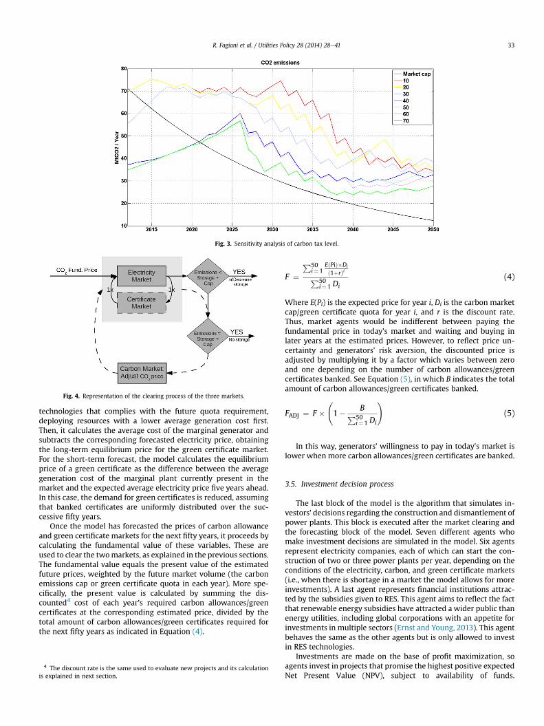
Fig. 3. Sensitivity analysis of carbon tax level.

Fig. 4. Representation of the clearing process of the three markets.


technologies that complies with the future quota requirement,deploying resources with a lower average generation cost first.Then, it calculates the average cost of the marginal generator andsubtracts the corresponding forecasted electricity price, obtainingthe long-term equilibrium price for the green certificate market.For the short-term forecast, the model calculates the equilibriumprice of a green certificate as the difference between the averagegeneration cost of the marginal plant currently present in themarket and the expected average electricity price five years ahead.In this case, the demand for green certificates is reduced, assumingthat banked certificates are uniformly distributed over the suc-cessive fifty years.

Once the model has forecasted the prices of carbon allowanceand green certificate markets for the next fifty years, it proceeds bycalculating the fundamental value of these variables. These areused to clear the twomarkets, as explained in the previous sections.The fundamental value equals the present value of the estimatedfuture prices, weighted by the future market volume (the carbonemissions cap or green certificate quota in each year). More spe-cifically, the present value is calculated by summing the dis-counted4 cost of each year’s required carbon allowances/greencertificates at the corresponding estimated price, divided by thetotal amount of carbon allowances/green certificates required forthe next fifty years as indicated in Equation (4).

4 The discount rate is the same used to evaluate new projects and its calculationis explained in next section.

F ¼P50

i¼1EðPiÞ�Di

ð1þrÞiP50i¼1 Di

(4)

Where E(Pi) is the expected price for year i, Di is the carbon marketcap/green certificate quota for year i, and r is the discount rate.Thus, market agents would be indifferent between paying thefundamental price in today’s market and waiting and buying inlater years at the estimated prices. However, to reflect price un-certainty and generators’ risk aversion, the discounted price isadjusted by multiplying it by a factor which varies between zeroand one depending on the number of carbon allowances/greencertificates banked. See Equation (5), in which B indicates the totalamount of carbon allowances/green certificates banked.

FADJ ¼ F � 1� BP50

i¼1 Di

!(5)

In this way, generators’ willingness to pay in today’s market islower when more carbon allowances/green certificates are banked.

3.5. Investment decision process

The last block of the model is the algorithm that simulates in-vestors’ decisions regarding the construction and dismantlement ofpower plants. This block is executed after the market clearing andthe forecasting block of the model. Seven different agents whomake investment decisions are simulated in the model. Six agentsrepresent electricity companies, each of which can start the con-struction of two or three power plants per year, depending on theconditions of the electricity, carbon, and green certificate markets(i.e., when there is shortage in a market the model allows for moreinvestments). A last agent represents financial institutions attrac-ted by the subsidies given to RES. This agent aims to reflect the factthat renewable energy subsidies have attracted a wider public thanenergy utilities, including global corporations with an appetite forinvestments in multiple sectors (Ernst and Young, 2013). This agentbehaves the same as the other agents but is only allowed to investin RES technologies.

Investments are made on the base of profit maximization, soagents invest in projects that promise the highest positive expectedNet Present Value (NPV), subject to availability of funds.


Investments have a fixed capital structure of 40% equity (E) and 60%debt (D), and future cash flows are discounted using the WeightedAverage Cost of Capital (WACC), supposing in the base case scenarioa cost of equity (Ke) of 15%, a cost of debt (Kd) of 5% and a tax rate(Tax) of 30% (6).

WACC ¼ Ke � EE þ D

þ Kd � DE þ D

� ð1� TaxÞ (6)

For the sake of this analysis, investment decisions are simplybased on a stand-alone project evaluation and investors do notconsider portfolio effects or externalities caused by lower marketprices. This way, the model simulates a market without barriers toentry in which incumbents do not exercise market power and arenot protected from entry by new competitors. The model considersthe impact of fuel price uncertainty when calculating the profit-ability of alternative investment projects, reflecting how differenttechnologies are affected by fluctuating prices. This is done byconsidering a risk adjusted measure of the NPV. This approach alsoallows for incorporating the additional price risk that is introducedby quantity-based policy mechanisms, compared to price-basedmechanisms.

The model uses the Conditional Value at Risk (CVaR) as a mea-sure of risk (Rockafellar and Uryasev, 2000). The CVaR is defined asthe expected loss in cases when the NPV is lower than a given Valueat Risk (VaR). By definition, the probability that the NPV is lowerthan the VaR under a confidence level a is 1 � a. See Fig. 5.

The NPV is adjusted for risk by subtracting the CVaR from theexpected NPV, as indicated in (7).

NPVRiskAdj ¼ EðNPVÞ � b� CVaR (7)

The CVaR is multiplied by a risk-aversion factor b, which is aninput variable of the simulation that indicates investors’ risk pref-erence. A b of zero indicates risk-neutral investors while highervalues correspond to increasing levels of risk-aversion. For the basecase scenario of the simulation we assume investors to be risk-averse, applying a b of one.

To calculate the profit distribution and eventually the risk-adjusted NPV of each technology, the model first calculates theoptimal long-term generation capacity, based on average expectedfuture fuel prices (as discussed in the previous section). Then 3000fuel price scenarios are randomly generated using a Weibull distri-bution which is obtained from the shape of monthly natural gas andcoal price data from the International Monetary Fund and theWorldBank covering the period October 1998eDecember 2008. The modelclears the electricity, the green certificate, and the carbon allowance

Fig. 5. Graphic representation of VaR

markets in each fuel price scenario, obtaining 3000 long-term priceforecasts. The model also generates 3000 random short-term elec-tricity, green certificate, and carbon prices, based on past volatilityand short-term forecasts, assuming un-biased, uncorrelated normaldistributions. Finally, the model linearly interpolates between thecurrent, short-term, and long-term prices, obtaining 3000 annualprices scenarios. These are then used to calculate the expected NPVof each technology, taking into account the evolution of marginalcosts in each scenario and its impact on the merit order.

Generation companies also make decisions regarding thedismantling of existing power plants. The model assumes that afterreaching their expected service life, power plants are dismantledonce they experience two or three years of consecutive losses, withhalf the agents dismantling after two years of losses and the otherhalf after three.

4. Model simulations and results

4.1. Performance indicators

A simulation consists of nine model runs, each one representinga different policy combination as indicated in Table 2.

As a central metric to evaluate the simulation results we use theadditional cost of a policy to society, normalized to one unit ofelectricity generation (a MWh). To evaluate how the cost of a policyis distributed between different actors in the market, we divide theeffects of a policy into changes of welfare to consumers, producers,and government finances, as compared to a base case scenariowhere no policies are implemented (N-N). Additional revenues tomanufacturers are not considered here, since this would require adistinction between imports and national value added in the pro-duction of power plants, which is outside the scope of this work.The policy cost to society per MWh of produced electricity iscalculated as expressed in Equation (8).

PolicyCost ¼PT

t¼1 ðDElet �DEPt þ St � CtÞ=ð1þ rÞtPTt¼1 Et

½V=MWh�

(8)

DElet represents the difference in consumers’ electricity bills in yeart compared to the base case (N-N). This is calculated consideringthe change in the electricity price but without including the addi-tional cost of the RES subsidy. An increase in the electricity billcorresponds to a decrease in the social welfare. Secondly, DEPt in-dicates the difference in producer surplus, measured as the

and CVaR of a NPV distribution.

Fig. 6. Cost increments to society.


difference in the industry profits using the concept of EconomicProfit (EP). In this case, higher industry profits increase socialwelfare. The Economic Profit is defined as the part of profitsexceeding the required return on the book value of assets.

EP ¼ EBIT� ð1� TaxÞ � Book�WACC (9)

Here EBIT indicates the earnings before interest and taxes, Taxrepresents the tax rate, and book is the balance sheet value of apower plant.

Next, we calculate the cost of the renewable energy subsidy, thecarbon tax revenues and the auctions of CO2 credits.While the costsof renewable policies are sometimes included in the electricitytariffs and thus affect the electricity consumer price, for the sakeclarity we attribute the cost directly to the government. St repre-sents the cost of subsidizing RES in year t, while Ct is the govern-ment income from the carbon reduction policy. Finally, the overallpolicy cost to society is defined as the sum of each year’s policy costdiscounted to the present (using a social discount rate r of 3%),divided by the total electricity production over the simulatedperiod

PTt¼1 Et .

We define the efficiency and effectiveness of the investigatedpolicies with respect to the two policy goals of CO2 emissionsreduction and RES generation. We measure the effectiveness of thecarbon reduction goal by dividing the accumulated CO2 emissions

Fig. 7. Policy e

by the total emissions cap (over all the years under consideration)in the corresponding ETS-only scenario (thus the lower, the better).We measure effectiveness of the renewable production goal as thepercentage of renewable electricity production in the total elec-tricity production over the entire simulation period. Efficiency inreaching the carbon reduction goal is measured as the change in thepolicy cost to society (in absolute values, not per MWh) divided bythe tons of CO2 avoided, as compared to the scenario without anypolicy intervention. Similarly, the efficiency in reaching therenewable policy goals is defined as the change of the policy cost tosociety divided by the total renewable electricity production inMWh.

4.2. Policy effectiveness and efficiency

A ‘pure’ emission market (without a renewable energy policyinstrument) reaches its carbon reduction goals at a discounted costto society of 5.15 V/MWh over the simulation period. However, itmisses the carbon reduction aims in the final years of the simula-tion leading to high final CO2 prices (see also Fig. 8, with No RESsupport). This effect can be explained as the consequence of aninvestment cycle in low-carbon technologies. Temporarily lowcarbon prices and imperfect forecasting may attract insufficientinvestment in low-carbon technology for complying with the very

fficiency.


strict reduction target assumed for 2050. A tax (50e100V/ton) wasfound to achieve similar or even better efficiency at a slightly higherlevel of carbon emissions than a carbon market (4.95 V/MWh costto society, with a 14.9% overshoot of emissions over the entiresimulation period).

Like the carbon market, the green certificate market is effectivein reaching its RES deployment and production targets. It does so ata total cost to society of 8.68 V/MWhRES. This is less than the cost offeed-in tariffs due to the more gradual and controlled introductionof the cheapest RES technologies to the market in a certificatemarket. On the other hand, the feed-in mechanism introduces re-newables into the market more effectively, but the overall cost tosociety is higher due to its open-ended nature and more expensiveresources being subsidized. Feed-in tariffs cause electricity prices tobe lower, but this benefit is more than offset by the subsidy cost(See Fig. 6, which shows the terms of Equation (8)).

Nonetheless, feed-in tariffs out-compete green certificate mar-kets in terms of cost-efficiency if the tariff level is calculatedcorrectly. See Fig. 7. This is because renewables are introducedearlier, which leads to more RES production over the simulatedperiod. Moreover, the green certificate market introduces someinefficiency by providing the same price to all technologies. Thiscauses windfall profits for cheaper generators, which reducesefficiency.

Fig. 7 also indicates that pure carbon policies are not efficient inintroducing RES to the market. Similarly, pure renewable energypolicies demonstrate poor efficiency in reducing carbon emissions.When these policies are implemented together, overall policy costsincrease. As a result, each policy instrument becomes less efficienton its own. See Fig. 7. However, the policy goals of carbon reductionand renewable energy development complement each other, so thecosts of the policies do not simply add up: the total cost of the twopolicies together is far less than the sum of the individual policycosts, while reaching the same policy effectiveness, as can be seenin Fig. 6. This confirms that both policies are necessary to reachcarbon reduction and renewable energy targets efficiently.

4.3. Policy interactions

A feed-in tariff leads to strong initial investments in RES tech-nologies, which in turn reduce CO2 emissions leading to lower CO2prices. The expectation of increasing carbon prices is sufficient toachieve the CO2 reduction objectives over the modeled time hori-zon, although towards the end of the period, the emissions are

Fig. 8. The impact of renewable energy policy on

above the cap. However, assuming investors do not have such along time horizon would lead to more investments in carbonintensive technologies, jeopardizing the long-term emission target.

The combination of carbon and green certificate markets leadsto more stable and lower carbon prices in the emission tradingscheme. The investment cycle in low-carbon power plants, whichleads to high CO2 prices at the end of the simulation in the no-RESpolicy case, is dampened by the investment induced by the greencertificate market (cf. Fig. 8). The overall difference in the effec-tiveness in reducing CO2 emissions over the entire simulationperiod is quite small. Combining green certificate and carbonmarkets leads to a higher carbon reduction of about 5%, ascompared to a pure carbon market. See Table 11.

We would expect the effect of carbon policies on the greencertificate markets to be similar to that of renewable policies on acarbon market. Both a carbon tax and an emission trading schemeare found to lower the green certificate price. However, the greencertificate market is found to be more robust than the carbonmarket under our assumptions and prices only drop to zero to-wards the end of the simulation if enough certificates are availableto meet renewable energy targets of 2050, as can be seen in Fig. 9.

The green certificate price is more stable in combination witha carbon reduction policy, which eliminates price peaks. Incontrast to the relatively stable prices, investment in renewableenergy is subject to investment cycles, as becomes evident in thelower part of Fig. 9. The banking of green certificates allows for astable price despite these investment cycles. However, our as-sumptions about the long-term horizon of investors may be toooptimistic. If short-term considerations prevail in investmentsdecision, the volatility of the investment cycles may increase,which could cause the green certificate price to collapse to zeroperiodically.

4.4. Sensitivity analyses

In addition to the base case scenario, we tested the sensitivity ofthe results to the impact of different regulatory decisions on thesimulation by changing the following input variables:

� The long-term RES objective;� The feed-in tariff biasing factor;� The carbon tax level;� The long-term CO2 emission target for the carbon market.

CO2 Emissions and the carbon market price.


We tested the effect of macro-economic variables by runningthe base case and the policy sensitivity analyses under differenthypothesis about economic conditions by changing the followinginput variables:

� Electricity demand growth rate;� Investor risk-aversion;� The cost of equity;� The growth rates of fuel prices.

The input variables of the base scenario and the different policysensitivity analysis are summarized in Table 3. The CO2 tax isassumed to start from a value of 50 V/ton and constantly increasesto a price of 100 V/ton in 2050. For the sensitivity analysis, thestarting value of the carbon tax is changed to 30 and 70 V/ton,leaving the final price of 100 V/ton in 2050 unchanged. Withrespect to the RES objective, we assume a target of 65% renewableelectricity production for the base case scenario, at which point theregulator stops subsidizing renewable energy. Sensitivities are runwith limits of 50% and 80% market penetration.

The CO2 emissions target represents the long-term objectiveimposed by the regulator when a carbon market is in place. At theEuropean level, policy makers are discussing a reduction of 80e90%, compared to 1990 levels, in 2050. We use the 80% reductiontarget in the base case scenario and perform a sensitivity analysiswith the more stringent 90% limit. Finally, the feed-in tariff biasingfactor aims to reflect the regulator’s uncertainty in the estimation ofgeneration costs use to calculate the tariffs paid to renewablegenerators. In the base case scenario, the regulator adds a mark-upof 15% to the exact average generation cost to guarantee a certainreturn to investors so they prefer RES over conventional technol-ogies. The sensitivity analyses are run using a biasing factor of 5%and 25% to simulate the case of the regulator under- or over-estimating the exact costs.

With respect to macro-economic variables, we change the elec-tricity demand growth rate after 2020 from 1.9% to 1.7% in order toreflect a scenario in which energy efficiency measures are moreeffective. The demand growth rate before 2020 is not changed andassumed to be 1.5% in both scenarios. We also test the impact ofinvestor risk aversion on the simulation results by changing the CVaRweight factor (b) from 1 to 0, which implies that investors are risk-neutral. In order to study the impact of the cost of capital on invest-mentdecisions,werunsensitivityanalyseswithacostof equityof 10%

Fig. 9. The impact of carbon reduction policy on R

and 20%. Finally, we test the impact of fuel prices on our analysis bychanging the annual increase rate of each fuel price by �0.7%.

The result of this sensitivity analysis is measured in terms of thetotal cost to society and of the policy effectiveness. The results arepresented in the appendix. The impacts of the feed-in tariff biasingfactor and of the tax level were already discussed in the previoussection. The biasing factor was already optimized; a higher feed-intariff increases the subsidy cost without significantly affecting theeffectiveness of the policy, while a lower feed-in tariff performspoorly in terms of effectiveness. In case of a green certificate mar-ket, the effects of quota changes are straight-forward: a higher/lower quota leads to higher/lower subsidy cost and policy effec-tiveness. Similarly, a higher/lower carbon tax leads to higher/lowercarbon reduction effectiveness at a higher/lower cost to society. Onthe other hand, reducing the cap from 20% to 10% of 1990 emissionlevels only slightly affects the outcome of a carbon market.

Regarding the macro-economic parameters, renewable energysources can enter the electricity market more easily under a purecarbon policy scheme if fuel prices are high. The effect of a carbontax depends on fuel prices, but a high enough feed-in tariff iseffective in all scenarios.

Higher and lower interest rates for investments (WACC) mainlyaffect the cost to society of both carbon and renewable policies,since capital costs are higher for non-renewable low carbon tech-nologies, such as CCS, and renewable technologies, than for con-ventional generation. So the costs to society rise with rising interestrates, as expected, because financing becomes more expensive.

The high efficiency scenario does not have a significant impacton the results because they are normalized to electricity produc-tion. An exception is represented by the green certificate market,the cost of which reduces because less expensive technologies arerequired to comply with the lower certificate demand.

If investors are assumed to be risk-neutral, this has several ef-fects. Firstly, the overall policy cost of the green certificatemarket alone is lower in the risk-neutral case than in the base casebecause generators demand a lower risk premium. Secondly, an ETSwithout a renewable support achieves far higher volumes ofrenewable electricity than the base case scenario. The explanationfor this lies in the higher market risk that renewable generatorsface, since they are not naturally hedged against fuel-price inducedelectricity price movements, as for example are gas power plants(Roques et al., 2008). The effectiveness of feed-in tariffs is notaffected by investor risk aversion because this mechanism

ES production and the green certificate price.

Table 4Base case scenario.

RES policy None Feed-in tariff Green certificatemarket

CO2 policy None Pig. Tax ETS None Pig. Tax ETS None Pig. Tax ETS

Base case 0.00 4.95 5.15 12.90 13.18 13.15 8.68 9.95 10.58High Pig. Tax e 5.36 e e 13.13 e e 10.40 e

Low Pig. Tax e 3.81 e e 13.26 e e 9.04 e

Low ETS Cap e e 4.79 e e 13.11 e e 11.57High FIT e e e 16.61 14.70 14.46 e e e

Low FIT e e e 5.53 9.76 8.45 e e e

High RES Obj. e e e 15.01 14.37 14.57 10.84 11.40 11.72Low RES Obj. e e e 10.57 11.55 11.80 8.02 8.58 9.10

Table 5High efficiency scenario.






Low FIT e e e 5.77 9.71 7.88 e e e



eliminates price risk in our analysis. However, due to the lowerelectricity price caused by a higher level of investments, the policycost of feed-in tariffs is higher in this case.

After presenting these sensitivity analyses, we now explainthe limitations of our model. First of all, we do not truly repre-sent the intermittence of some RES in the model, so their inte-gration cost and impact on dispatchable generators may beunderestimated. In addition, we assume that investors consider avery long time horizon, while actual companies appear moreoriented towards the short term. This would lead to more volatilemarket prices and perhaps more cyclical investment behaviorthan we observe.

5. Conclusions

Wepresent an agent-basedmodel that reproduces the evolutionof a power sector, loosely based on Spain, between 2012 and 2050.We simulate how the investment decisions of risk-averse, profit-maximizing generating companies are affected by carbon reductionand renewable energy policies. The goal of this paper is to inves-tigate the dynamic interactions between these two policies.

Our analysis suggests a single policy is not a cost-efficient way ofachieving both a reduction of CO2 emissions and an increase inrenewable electricity generation. Hence, the decision of the Euro-pean Commission and of national governments to introducerenewable energy support mechanisms in addition to the EU ETS issensible because it reduces the total cost of achieving a more sus-tainable electricity sector. This finding corroborates what Linareset al. (2008) found with an equilibrium model. We found that thecombination of carbon reduction and renewable energy policiesleads to lower and more stable costs for both policies.

However, while the introduction of a carbon reduction mecha-nism has limited effect on a green certificate market, renewableenergy policy has a stronger impact on a carbon market. A highvolume of renewable electricity generation could lead to low pricesin carbonmarkets, as has been the practical experience with the EUETS and recognized in the literature. Our model indicates that thereis also an adverse long-term dynamic effect, namely that low car-bon prices may attract investment in coal-fired generators, whichcould lock the electricity sector into a pathway of higher futureemissions (as appears to have happened in the Netherlands).

To avoid periods of low carbon prices, regulators may opt for ahybrid policy instrument such as a carbon price floor. The UKintroduced a national price floor for carbon, within the EU ETSframework, in April 2013. If set high enough above the market pricefor carbon, a price floormay effectively function as a carbon tax. Thequestion whether such hybrid instruments work well meritsfurther research.

Our analysis demonstrates how difficult it is for policy makers toestimate the optimal level of a price-based policy. However, quantity-based mechanisms may also result in a price which does not satisfythe regulator because is too high or too low. We observe that bothprice and quantity policies may perform poorly when they areimplemented using static parameters, as the dynamic changes toexternal conditions affect the prices and effectiveness of the policies.

A solution may be provided by adaptive policy making. Withrespect to the carbon market, policy makers may intervene bylowering the emission cap faster/slower if the price is too low/high,in an attempt to keep the price within a certain accepted level. Thisway, an aggressive renewable energy policy would contribute to anearly achievement of carbon reduction targets, rather than in lowcarbon costs for fossil fuel plant. An example may be found in theJuly 2013 decision of the European Parliament to temporarilyreduce the number of allowances auctioned for the EU ETS (back-loading), although this was not part of a structural policy.

Nonetheless, policy makers should avoid frequent and unpre-dictable policy changes as this would contribute to regulatory un-certainty, which in general discourages investment in the energysector (Fagiani and Hakvoort, 2014). A solution is to bind policyadaptations to predictable rules, for instance to announce thatbackloading will take place if the carbon price is below a certainlevel. Another example of how regulatory uncertainty could belimited is to reduce the number of carbon allowances as a functionof renewable electricity production. In practice, the regulator could,for example, calculate the reduction in carbon emissions obtainedby one MWh of renewable electricity substituting conventionaltechnologies, decreasing adequately the cap of the carbon market.The carbon equivalent of one MWh of renewable electricity woulddepend on the carbon intensity of the electricity sector, moreprecisely on which power plants the RES substitute in the meritorder curve, which might be difficult to estimate. However, bydoing so the regulator could offset the negative impact of renew-able energy policy on the carbon market, obtaining a mechanismthat would be more robust to the dynamic evolution of the elec-tricity sector. If such an announced dynamic adjustment of emis-sion caps is effective and feasible in practices is another topic forfuture research.

Acknowledgments

Riccardo Fagiani and JörnC. Richsteinhave been awardedErasmusMundus Joint Doctorate Fellowships. The authors would like to ex-press their gratitude towards all partner institutions within the pro-gram as well as the European Commission for their support.

APPENDIX

Additional Cost to society (V/MWh)

Table 6High fuel price scenario.






Low FIT e e e 6.15 10.11 9.11 e e e


Table 7Low fuel price scenario.






Low FIT e e e 5.29 8.29 8.16 e e e


Table 8Risk-neutral scenario.






Low FIT e e e 6.33 9.99 10.11 e e e


Table 9High weighted average cost of capital scenario.






Low FIT e e e 6.26 9.82 9.41 e e e



RES policy None Feed-In tariff Green certificatemarket


Base case 4.13 1.15 1.04 1.58 0.44 0.87 3.18 0.91 0.99High Pig. Tax 4.13 1.04 e e 0.43 e e 0.86 e

Low Pig. Tax 4.13 1.56 e e 0.54 e e 1.24 e

Low ETS Cap 4.13 e 1.05 e e 0.79 e e 1.00High FIT 4.13 e e 1.58 0.43 0.87 e e e

Low FIT 4.13 e e 3.67 0.84 1.09 e e e

High RES Obj. 4.13 e e 0.86 0.33 0.63 2.86 0.84 0.94Low RES Obj. 4.13 e e 2.36 0.53 0.90 3.66 0.98 1.02

Table 10Low weighted average cost of capital scenario.






Low FIT e e e 4.70 8.92 7.69 e e e



Carbon Reduction Effectiveness (ratio of emissions compared toscenario cap).







Low FIT e e e 3.60 0.86 1.06 e e e








Low FIT e e e 3.45 0.81 1.08 e e e








Low FIT e e e 3.75 0.93 1.08 e e e








Low FIT e e e 3.72 0.85 1.09 e e e





Base case 0.25 0.28 0.35 0.80 0.81 0.80 0.48 0.50 0.51High Pig. Tax 0.25 0.36 e e 0.81 e e 0.50 e

Low Pig. Tax 0.25 0.27 e e 0.81 e e 0.49 e

Low ETS Cap 0.25 e 0.37 e e 0.80 e e 0.49High FIT 0.25 e e 0.81 0.82 0.81 e e e

Low FIT 0.25 e e 0.38 0.39 0.40 e e e

High RES Obj. 0.25 e e 0.93 0.92 0.92 0.55 0.57 0.56Low RES Obj. 0.25 e e 0.65 0.66 0.65 0.42 0.43 0.43







Low FIT e e e 0.40 0.40 0.41 e e e








Low FIT e e e 3.62 1.00 1.13 e e e








Low FIT e e e 3.62 0.82 1.01 e e e


RES Production Effectiveness (percentage of electricity produced byRES).








Low FIT e e e 0.38 0.40 0.42 e e e








Low FIT e e e 0.40 0.39 0.41 e e e








Low FIT e e e 0.38 0.39 0.41 e e e








Low FIT e e e 0.39 0.39 0.40 e e e








Low FIT e e e 0.40 0.42 0.42 e e e



References

Amundsen, E.S., Nese, G., 2009. Integration of tradable green certificate markets:what can be expected? J. Policy Model. 31, 903e922.

Chappin, E.J.L., 2011. Simulating Energy Transitions. PhD Thesis. Delft University ofTechnology, Delft.

Chappin, E., Dijkema, G., de Vries, L., 2010. Carbon policies: do they Deliver in thelong run? In: Sioshansi, F.P. (Ed.), Generating Electricity in a Carbon-constrainedWorld. Academic Press, pp. 31e56 (Ch. 2).

De Jonghe, C., Delarue, E., Belmans, R., D’haeseleer, W., 2009. Interactions betweenmeasures for the support of electricity from renewable energy sources and CO2mitigation. Energy Policy 37, 4743e4752.

Del Rio, P., 2012. The dynamic efficiency of feed-in tariffs: the impact of differentdesign elements. Energy Policy 41, 139e151.

Ernst, Young, 2013. Renewable Energy Country Attractiveness Indices.European Commission, 2009. Directive 2009/28/EC (Brussels).European Commission, 2010. COM(2010) 639 def.: Energy 2020 a Strategy for

Competitive, Sustainable and Secure Energy (Brussels).European Commission, 2011. COM(2011) 885 def.: Energy Road Map 2050

(Brussels).Fagiani, R., Barquin, J., Hakvoort, R., 2013. Risk-based assessment of the cost-

efficiency and the effectivity of renewable energy support schemes: certifi-cate markets versus feed-in tariffs. Energy Policy 55, 648e661.

Fagiani, R., Hakvoort, R., 2014. The role of regulatory uncertainty in certificatemarkets: a case study of the Swedish/Norwegian market. Energy Policy 65,608e618.

Gross, R., Blyth, W., Heptonstall, P., 2010. Risks, revenues and investment in elec-tricity generation: why policy needs to look beyond costs. Energy Econ. 32,796e804.

Grubb, M., Newberry, D., 2007. Pricing Carbon for Electricity Generation: Nationaland International Dimension (Working paper).

Haas, R., Panzer, C., Resch, G., Ragwitz, M., Reece, G., Held, A., 2011. A historicalreview of promotion strategies for electricity from renewable energy sources inEU countries. Renew. Sustain. Energy Rev. 15, 1003e1034.

Hepburn, C., 2006. Regulation by prices, quantities, or both: a review of instrumentchoice. Oxf. Rev. Econ. Policy 22, 226e247.

Jensen, S.G., Skytte, K., 2003. Simultaneous attainment of energy goals by means ofgreen certificates and emission permits. Energy Policy 31, 63e71.

Lecuyer, O., Quirion, P., 2013. Can Uncertainty Justify Overlapping Policy In-struments to Mitigate Emissions?.

Linares, P., Javier Santos, F., Ventosa, M., 2008. Coordination of carbon reduction andrenewable energy support policies. Clim. Policy 8, 377e394.

Menanteau, P., Finon, D., Lamy, M.-L., 2003. Prices versus quantities: choosing po-lices for promoting the development of renewable energy. Energy Policy 31,799e812.

Olsina, F., Garces, F., Haubrich, H.J., 2006. Modeling long-term dynamics of elec-tricity markets. Energy Policy 34, 1411e1433.

Rathmann, M., 2007. Do support systems for RES-E reduce EU-ETS-driven electricityprices? Energy Policy 35, 342e349.

Red Electrica de Espana, 2012. El sistema electrico espanol 2011 (Madrid).Richstein, J., Chappin, E., De Vries, L., 2012. Impacts of the introduction of CO2 price

floors in a two-country electricity market model. In: 12th IAEE European PhD-students Day. Venice, 2012.

Rockafellar, R.T., Uryasev, S., 2000. Optimization of conditional value-at-risk. J. Risk2, 21e41.

Roques, F.A., Newbery, D.M., Nuttall, W.J., 2008. Fuel mix diversification incentivesin liberalized electricity markets: a mean-variance portfolio theory approach.Energy Econ. 30, 1831e1849.

Simon, H.A., 1957. Models of Man: Social and Rational. John Wiley and Sons, NewYork.

Swedish Energy Agency, 2012. The Electricity Certificate System.Tinbergen, J., 1952. On the Theory of Economic Policy, second ed. North-Holland

Publishing Company, Amsterdam.Weitzman, M.L., 1974. Prices vs. quantities. Rev. Econ. Stud., 477e490.

http://refhub.elsevier.com/S0957-1787(13)00072-6/sref1
















































































Documents

The dynamic impact of carbon reduction and renewable support policies on the electricity sector