Cost-Effectiveness of Renewable Electricity Policies · Cost-Effectiveness of Renewable Electricity Policies ... renewable energy, electricity, renewable portfolio standard, ... often

1616 P St. NW Washington, DC 20036 202-328-5000 www.rff.org

January 2005 RFF DP 05-01

Cost-Effectiveness of Renewable Electricity Policies

Karen Pa lmer and Da l l as Bur t raw

DIS

CU

SSIO

N P

APE

R

© 2005 Resources for the Future. All rights reserved. No portion of this paper may be reproduced without permission of the authors. Discussion papers are research materials circulated by their authors for purposes of information and discussion. They have not necessarily undergone formal peer review.


Karen Palmer and Dallas Burtraw

Abstract We analyze policies to promote renewable sources of electricity. A renewable portfolio

standard raises electricity prices and primarily reduces gas-fired generation. A “knee” of the cost curve exists between 15% and 20% goals for 2020 in our central case, and higher natural gas prices lower the cost of greater reliance on renewables. A renewable energy production tax credit lowers electricity price at the expense of taxpayers and thus limits its effectiveness in reducing carbon emissions; it also is less cost-effective at increasing renewables than a portfolio standard. Neither policy is as cost-effective as a cap-and-trade policy for achieving carbon emissions reductions.

Key Words: renewable energy, electricity, renewable portfolio standard, carbon dioxide

JEL Classification Numbers: Q42, Q48, Q54

Contents

1. Introduction......................................................................................................................... 1

2. Policies to Promote Renewables ........................................................................................ 2

3. Model Framework .............................................................................................................. 4

4. Policy Scenarios and Sensitivity Analysis ......................................................................... 6

RPS Scenarios..................................................................................................................... 7

REPC................................................................................................................................... 8

Carbon Policy with Updating Allowance Allocation Based on Output ............................. 8

5. Results for Central Case Baseline and Alternatives ........................................................ 9

6. Results for the RPS ........................................................................................................... 10

Prior Studies...................................................................................................................... 12

Welfare Effects of RPSs ................................................................................................... 13

Sensitivity Analysis for the 15% RPS .............................................................................. 14

7. Results for REPC .............................................................................................................. 16

Comparing Welfare Effects of RPS and REPC Policies .................................................. 17

8. Carbon Cap with Allowance Allocation on the Basis of Generation ........................... 18

9. Conclusions........................................................................................................................ 19

References.............................................................................................................................. 21

Figures.................................................................................................................................... 24

Tables ..................................................................................................................................... 28


Karen Palmer and Dallas Burtraw∗

1. Introduction

The electricity sector is a major source of the carbon dioxide emissions that contribute to global climate change. In the United States, electricity generators fired by fossil fuels are responsible for roughly 40% of all carbon dioxide emissions resulting from human activity. Switching a substantial fraction of U.S. electricity-generating capacity from fossil fuels to renewable sources such as geothermal, biomass, or wind-powered turbines would help reduce carbon emissions from this sector. Nonetheless, because of their relatively high cost, nonhydroelectric renewables remain only 2% of total electricity generation (McVeigh et al. 2000).

In theory, one way to motivate a shift away from fossil fuels toward renewables would be to tax or cap carbon emissions from electricity generators. However, U.S. policymakers have not embraced carbon taxes or a cap-and-trade approach as a means of controlling greenhouse gas emissions. Proponents of strict limits on greenhouse gas emissions recognize that a “slow, stop, reverse” approach to carbon mitigation may be necessary to win political support. This approach has much to recommend it, given the uncertainties surrounding the costs and benefits of reducing greenhouse gas emissions, but it limits the possibilities for learning by doing in the near term. Political preference for the go-slow approach on carbon policies suggests that a policy aimed directly at increasing renewables may be necessary to realize gains from learning and substantially increase contributions from renewables—and thus to achieve higher emissions-reduction goals in the long term.

This research analyzes the effects of the two leading government policies designed to increase the contribution of renewables to total U.S. electricity supply. One approach that has been popular is tax credits for certain types of renewables, known at the federal level as the Renewable Energy Production Credit (REPC). A second approach adopted in a number of states—including Connecticut, Maine, Nevada, Massachusetts, New Jersey, and California—is a requirement, known as a renewable portfolio standard (RPS), that a minimum percentage of the electricity produced or sold in the state come from renewable sources, typically excluding hydroelectric facilities. A number of bills proposing national portfolio standards of 5% to 20%

∗ Palmer ([email protected]) and Burtraw ([email protected]) are both Senior Fellows at Resources for the Future.

1

Resources for the Future Palmer and Burtraw

by deadlines ranging from 2010 to 2020 have been before the U.S. Congress in recent years, but none have been passed into law.

We consider the effects of these policies on costs, utility investment decisions, the mix of technologies and fuels used to generate electricity, and renewable generation by region. We also analyze the effects of these policies on electricity prices and on carbon emissions from electricity generators. Finally, we look at the effects of different technological assumptions, the role of learning, and the role of fuel price assumptions.

In brief, we find the RPS policy is more cost-effective than the REPC as a means of both increasing renewables and reducing carbon emissions. We find the cost of the RPS in terms of changes in electricity price or social cost to be relatively low at levels up to 15% penetration of the electricity grid by 2020; however, the price rises dramatically for a penetration target of 20%. Natural gas prices are inversely related to the cost of achieving renewable generation. The RPS tends to encourage renewables largely at the expense of natural gas and thus is less effective at reducing carbon emissions than would be a direct tax on carbon emissions.

2. Policies to Promote Renewables

Worldwide, within the countries of the Organisation for Economic Co-operation and Development as well as within the United States, nonhydro renewables account for about 2% of total electricity generation. However, most developed countries are hoping to increase renewable generation dramatically over the next 30 years, and a number of countries have implemented policies to help them to achieve these goals (Darmstadter 2003, Palmer and Burtraw 2004). We examine in detail two policy approaches that stand out as arguably the most widely considered and used. One is a tax credit that directly subsidizes specified technologies; the other is a portfolio standard, often with a flexible credit-trading component, that requires a minimum level of renewables-based generation.

The production tax credit has been the main policy employed at the federal level in the United States. In 1992, the U.S. Congress authorized a production tax credit (known as the REPC) of 1.5 cents/kWh of electricity produced from wind and dedicated closed-loop biomass generators.1 The REPC applied to new generators for the first 10 years of their operation. The REPC was extended in 2001 and indexed to inflation in subsequent legislation. It was extended again in 2004 through the end of 2005 and expanded to include geothermal, solar energy, and

1 A closed-loop biomass system involves a source of biomass fuel dedicated to energy production. A dedicated biomass facility is one that burns biomass only. In contrast, an open-loop biomass system could use biomass waste from other economic activities at a dedicated biomass facility or at a facility that also uses fossil fuel.

2


landfill gas. In addition to this production incentive, the federal government has a tax credit for investment in geothermal and solar generators equal to 10% of the capital cost of the generating facility; this credit has no expiration date.

The second policy we analyze, a portfolio standard, is observed at the state level in the United States and in many European countries. Since the mid-1990s, 16 states have imposed renewable generation requirements on electricity retailers or generators within their borders.2 Typically referred to as RPSs, these requirements set a minimum level or percentage of electricity sales that must come from renewable generation by a particular date. In several states, including Connecticut, Nevada, New Jersey, New Mexico, Texas, and Wisconsin, the implementing RPS law or regulation also allows for trading of renewable energy credits to meet this requirement. Thus, an electricity retailer can meet its renewable obligation by generating renewable energy itself and keeping the associated credits, purchasing renewable energy bundled with credits from others, or purchasing renewable energy credits sold separately. In New Mexico and Nevada, solar generators receive more than one credit per kilowatt-hour produced, providing them with an additional incentive above other renewables.

In the European Union, a similar policy took shape under the Renewables Directive in October 2001, which required member states to adopt national targets consistent with reaching the overall E.U. target that 12% of total energy and 22% of all electricity come from renewables by 2010.3 Several countries, including the United Kingdom, Sweden, Belgium, and Italy, have implemented tradable certificates to achieve their national goals (Energy Research Centre of the Netherlands 2004). The European Union is also studying the feasibility, costs, and benefits of implementing a community-wide trading program (ESD 2001, Quené 2002). Australia adopted an RPS for wholesale electricity suppliers beginning in 2001.4 Japan also has an RPS that includes a price cap of 11 yen/kWh on the price of renewable credits (Keiko 2003).

There are myriad other programs that we do not examine. One approach imposes a surcharge on electricity consumption and the revenue is distributed in periodic auctions that allow producers of renewable energy to bid for subsidies per kilowatt-hour (Wiser et al. 2003). Given the limited success of the subsidy auction, California decided to supplement this policy with an RPS in 2002. In Europe a similar approach is the competitive tender offer or bidding

2 For more details on state RPS policies, see the Union of Concerned Scientists website (http://www.ucsusa.org/publication.cfm?publicationID=68). New York is the 17th state to adopt an RPS, which is scheduled to start to take effect in January 2006. For a review of the initial experience with the Texas program, see Lagniss and Wiser (2003). 3 Different targets are set for different member states based on current renewable generation and potential resources available locally. 4 For more information, see http://www.orer.gov.au (accessed February 21, 2003).

3


system, wherein an agency or utility bids to supply renewable energy of particular types for many years (typically 15 or 20) into the future.5 Bids often take the form of the minimum price of electricity (per kilowatt-hour) that a renewable supplier needs to supply electricity. One other approach used in Germany, France (for wind power only), Finland, and Denmark, among other places, is a price guarantee for renewables, often referred to as a feed-in tariff.6 This approach is similar to that formerly used in the United States under the Public Utility Regulatory Policies Act adopted in 1978; it was known as a standard offer contract. In addition, many U.S. states use net metering to enable a customer who generates electricity for his or her own use to sell any excess back to the electricity supplier at the retail price.

3. Model Framework

This paper makes several important contributions to the existing literature. It is the first study to compare RPS policies in a common framework using common underlying assumptions. It is also one of the first to analyze the effects of extending the REPC into the future and the first to compare this approach with an RPS.7 We look at a more general REPC that subsidizes the same set of renewable technologies that are covered by the RPS in a manner designed to achieve the same quantity of renewable generation as a 15% RPS. Unlike prior studies, this study measures the economic surplus effects of different policies. We also look at the effects of different national policies on regions. Finally, we contrast the RPS policy with a carbon cap-and-trade program that uses carbon allowance allocation as a method of encouraging the use of low-emitting and non-carbon-emitting generating technologies to see how the two compare in terms of promoting renewables use and other measures.

5 The New York State RPS policy will use a central procurement auction of this type run by a state agency to achieve its renewables goal instead of imposing a minimum renewables requirement on private electricity suppliers in the state. 6 Denmark had planned to replace the feed-in tariff system with a tradable credit approach in January 2003, but that change has been postponed indefinitely because of concerns among renewable generators about the effectiveness of the green certificate market in promoting renewables. Germany’s initial feed-in tariff law took effect in 1990 and was reenacted in 2000 to help Germany achieve its goal of doubling renewables share from 6% to 12% by 2010. 7 In the 2004 Annual Energy Outlook, U.S. EIA (2004) presents a policy analysis that considers three approaches to extending the REPC. One variation extends the existing credit through 2006 and expands it to include open-loop biomass and landfill gas generation. A second variation expands the coverage of the credit similarly and extends it through the end of 2012. A third variation cuts the value of the tax credit in half and extends it through 2012. EIA finds that all of the policies have their biggest effect on wind generation, followed by dedicated biomass, with much smaller impacts on municipal solid waste and landfill gas and on biomass cofiring. The policies all lead to higher electricity generation in 2010 (implying lower prices, although effects on electricity prices are not reported).

4


Numerical simulations are performed using the Haiku electricity market model to simulate equilibrium in regional electricity markets in the United States, including interregional electricity trade with an integrated algorithm for sulfur dioxide (SO2), nitrogen oxides (NOx), and mercury emissions-control technology choice.8 The model calculates electricity demand; electricity prices; composition of electricity supply; interregional electricity trading activity; and emissions of major pollutants such as NOx, SO2, carbon dioxide (CO2), and mercury from electricity generation in 13 regions, for four time periods in three seasons. For each of these 156 segments of the electricity market, demand is aggregated from price-responsive demand schedules for three customer classes: residential, industrial, and commercial. Supply is aggregated from the complete set of electricity plants in the United States, which for modeling purposes are aggregated into 48 representative plants in each region. Investment in new generation capacity and retirement of existing facilities are determined in a dynamic framework, based on capacity-related costs of providing service in the future. Generator dispatch in the model is based on the minimization of short-run variable costs of generation.

Interregional power trading is identified as the level of trading necessary to equilibrate regional electricity prices (accounting for transmission costs and power losses) subject to the level of available interregional transmission capability as reported by the North American Electric Reliability Council (NERC). Factor prices, such as the cost of capital and labor, are held constant. Fuel price forecasts are calibrated to match U.S. Energy Information Administration (EIA) price forecasts from the Annual Energy Outlook 2003 (EIA 2002a) and varied in sensitivity analysis. Fuel market modules for coal and natural gas calculate prices that are responsive to factor demand. Coal is differentiated along several dimensions, including fuel quality and location of supply, and both coal and natural gas prices are differentiated by point of delivery.

The model allows new additions of four types of renewable generators: wind turbines, biomass gasification combined cycle, geothermal, and landfill gas. Resource availability at particular cost levels is specified for each of the 13 regions in the model. Geothermal resources are limited to the southwestern section of the continental United States. The generating potential of the wind resource varies substantially across regions, largely as a function of wind speed. The cost of tapping that wind resource to generate electricity also varies greatly with land use, terrain, and distance to the transmission grid. Biomass generation depends on the nature of the fuel supply curve within a particular region. Landfill gas resources depend on methane yield from

8 Haiku was developed by RFF and has been used for a number of reports and articles that appear in the peer-reviewed literature. The model has been compared with other simulation models as part of two series of meetings of Stanford University’s Energy Modeling Forum (1998, 2001).

5


different classes of landfills and associated costs. Information for resource availability and other technical characteristics is taken from a variety of sources but primarily from EIA.

We make several assumptions about underlying policies, both environmental and market regulatory, that affect the performance of electricity generators. We assume that electricity generators face an annual cap on SO2 emissions as a result of Title IV of the 1990 Clean Air Act Amendments and that there is a seasonal cap on NOx emissions in all of the regions that include states covered by the U.S. Environmental Protection Agency’s NOx SIP Call.9 We assume electricity generators face no requirements to reduce mercury emissions or emissions of CO2. We include all announced New Source Review (NSR) settlements in our technical assumptions about emissions control at existing generators.10 We do not include state-level multipollutant policies, such as those in New York and North Carolina.

In our central case, we assume the REPC for dedicated biomass and wind generation is phased out between 2005 and 2010.11 We also include a perpetual 10% tax credit for investment in new geothermal resources, but we do not include any state-level RPS policies.

We assume that prices in the electricity market are set competitively in six NERC regions—New York, New England, Mid-Atlantic (MAAC), Illinois area (MAIN), Ohio Valley (ECAR), and Texas (ERCOT)—and that there is time-of-day pricing for industrial customers in these regions. In all other regions of the country, we assume that prices are set according to cost-of-service regulation at average cost. We simulate the model through 2020 and extrapolate our results to 2030 for purposes of calculating returns to investment choices. We report results for 2020. All costs and prices are expressed in 1999 real dollars.

4. Policy Scenarios and Sensitivity Analysis

We focus on two types of policies to promote renewables and one policy aimed at reducing CO2 emissions:

• a series of increasingly stringent RPSs,

9 Because of the availability of the emissions allowance bank built up between 1995 and 2000, actual emissions of SO2 exceed the level of the cap until 2012. We model this drawdown of the bank exogenously using information from the U.S. Environmental Protection Agency and EIA. 10 NSR settlements are those that electricity-generating companies have reached with the federal government to bring their plants into compliance with New Source Review requirements for emissions reductions that the government asserts were violated by past investments at specific facilities. 11 In practice, facilities that qualify receive the credit for 10 years. In our model, they receive the credit indefinitely, but only as long as the credit is active.

6


• a production incentive (tax credit) for renewables (REPC), and

• a carbon cap-and-trade program that uses an updating approach to allocation of emissionsallowances to reward generation from relatively clean technologies.

RPS Scenarios

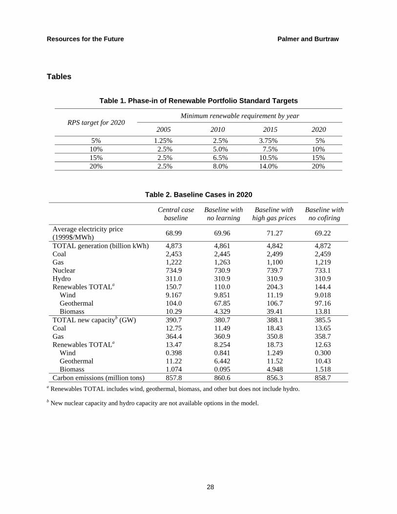
We analyze a series of national RPS targets ranging from 5% to 20% that phase in between 2005 and 2020, as shown in Table 1. A stylized illustration of how the RPS credit affects the variable cost (V) for renewable (r) and nonrenewable (n) generators is the following. If marginal cost of generation is (C), the RPS credit price is (p), and the renewable target is (t),

then and 1n n r r

tp V C pt

⎛ ⎞= + ∗ = −⎜ ⎟−⎝ ⎠V C . That is, the variable cost of the nonrenewable

generators is increased by the permit price multiplied by the target, which is a percentage less than one, and the variable cost of the renewable generator is decreased by the value of a permit.

The renewable technologies covered by the standard include existing solar and municipal solid waste generation and both new and existing dedicated biomass, biomass cofiring in coal-fired generators, geothermal, and wind. For each kilowatt-hour of electricity generated using one of these technologies, a renewable energy credit is created, and these credits are assumed to be tradable in a national credit-trading market. It means that there may be some geographic concentration of renewable generation in regions with greater access to abundant and low-cost renewable resources, and these regions may become exporters of renewable credits and, in some cases—depending on transmission constraints—of electricity as well.

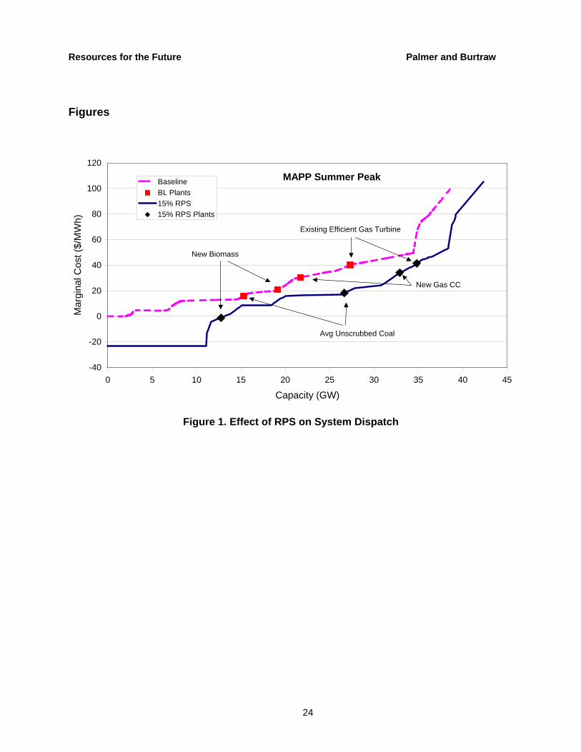
Figure 1 illustrates the effect on the schedule of variable costs for a region with ample renewable resources, the Mid-Continent Area Power Pool (MAPP) electric reliability region (including the northern plains states). The horizontal axis depicts the amount of installed capacity in 2020 and the vertical axis represents variable costs. The broken line is the variable cost schedule in the baseline with a sample of technologies indicated, and the solid line is the schedule under a 15% RPS. Two effects are evident in the figure. First, the cost of nonrenewable technologies goes up, although least of all for the unscrubbed coal plant that can cofire with biomass to partially satisfy the renewable requirement. Second, most existing technologies are pushed to the right in the schedule as new renewables enter and typically have lower variable costs. A large segment of wind capacity actually has negative cost, reflecting very low operating costs and the after-tax value of the RPS credits. In this region the renewable share of total generation approaches 40%, and the region is an exporter of RPS credits.

The costs and other effects of the national RPS analysis are likely to depend on several underlying assumptions, including the ability to cofire coal plants with biomass and whether those cofired kilowatt-hours are covered by the RPS program, the underlying price of natural

7


gas, the importance of learning in determining future capital costs of all new technologies, and whether the RPS is coupled with an REPC (see below). We include several sensitivities of the 15% RPS scenario measured against a relevant baseline to investigate how changing these assumptions affects the way the industry responds.

REPC

We model two versions of a REPC policy. The first, REPC-E, represents an extension of a policy that grants a federal income tax credit of 1.7 cents (in real dollar terms)/kWh, amounting to an after-tax subsidy of 2.8 cents, for electricity generated using either wind or closed-loop biomass technology. When the production incentive is extended in the model, we assume it applies to all future generation across the entire forecast horizon.

The second, REPC-G, is a general production tax credit policy that comprises all the technologies eligible for renewable credits covered under an RPS in the model. We identify the levels of a production tax credit in each simulation year that provide an after-tax subsidy equivalent to the phased-in 15% RPS policy. In the case of the RPS, the source of the subsidy is effectively a tax on fossil fuel, hydro, and nuclear generation. In the case of the REPC-G, the source of the subsidy is federal tax dollars. Analyzing this scenario provides a means for directly comparing the effects of the two instruments, a tax credit and a tradable portfolio standard, set to achieve a common effective subsidy.

Carbon Policy with Updating Allowance Allocation Based on Output

A carbon tax or carbon cap-and-trade program could be designed to encourage the use of renewables and other low-emitting technologies.12 One approach, embodied in federal multipollutant legislation proposed by Sen. Tom Carper (D-DE), is to allocate emissions allowances on the basis of electricity generation to all generators, including renewables, regardless of whether they emit carbon. Under this approach, each generator’s share of the total annual amount of carbon emissions allowances would depend on its share of electricity generation in a recent year. This approach provides a subsidy for increasing generation, and the subsidy is particularly effective for renewables, since they have no emissions.13 It also is

12 Placing a tax on carbon emissions or imposing a carbon cap-and-trade program arguably will create an incentive to adopt renewables, which have no carbon emissions. The point here is to impose policies that go even further to create an advantage for using renewables. 13 An important consideration in determining the effect of this implicit subsidy is the way in which prices are determined and the nature of regulation at the state level (Burtraw et al. 2001).

8


analogous to the revenue-neutral pollution tax on NOx that has been implemented in Sweden (Sterner and Hoglund 2000).

Such a policy could be implemented in many ways. Here, we consider two approaches:

• allocating carbon emissionsallowances to all generators, excluding existing hydro and nuclear facilities, based on current-year generation and

• allocating carbon emissionsallowances to nonhydro renewable generators only, based on current-year generation.

To create comparability across policies, we set the level of the carbon cap for these runs in each year equal to the total amount of emissions under a 15% RPS.

5. Results for Central Case Baseline and Alternatives

First we present results first for the central case baseline and alternatives considered in sensitivity analysis. Next we present results for the RPS policies, including analysis of partial equilibrium welfare measures. We then present results for the REPC policies and compare them with the RPS. Last, we present results for the carbon cap-and-trade policy.

In the central case baseline, coal represents 50% of total generation in 2020. Generation by nonhydro renewables is forecast to be 3.1% of total generation, with the majority of that coming from geothermal. Natural gas accounts for roughly 93% of total new capacity brought on line by 2020. Total carbon emissions are projected to be 857.8 million tons.

Alternative baselines that are used in sensitivity analysis are reported in Table 2. The first has no capital cost learning. Capital costs of new technologies do not depend on the level of accumulation of new capacity, nor do they vary over time. This change reduces the future cost advantages of investing in new and less developed technologies, such as biomass gasification and geothermal, and thus leads to a lower level of generation from nonhydro renewables as a class and particularly from biomass and geothermal. Electricity price increases by 1%, and the shift away from renewables results in a slight increase in total carbon emissions.

The second alternative is the high gas price case, which assumes the price of natural gas is roughly 15% higher than in the central case baseline. One reason this scenario is compelling is the empirical observation that long-run gas prices that lock in through forward markets are consistently above long-run forecasts. Bolinger and Wiser (2003) conjecture that the difference is due to price risk stemming from short-run volatility. This scenario yields an electricity price that is 3% higher than in the central case baseline. The higher relative price of natural gas dampens gas generation to a level 9% below the central case baseline, but it results in more generation by coal and renewables. The changing mix of generation causes no real change in

9


total carbon emissions. The renewable share of total generation in the high-gas-price baseline in 2020 is 36% higher than in the central case baseline, but it remains at just 4.2% of total generation.

The third alternative is a baseline with no biomass cofiring at existing coal plants. Biomass cofiring is somewhat experimental, and the extent to which this technology will play out in the future is uncertain. Eliminating the cofiring option leads to an electricity price increase of less than 1% and slightly more generation with new dedicated biomass and new coal.

6. Results for the RPS

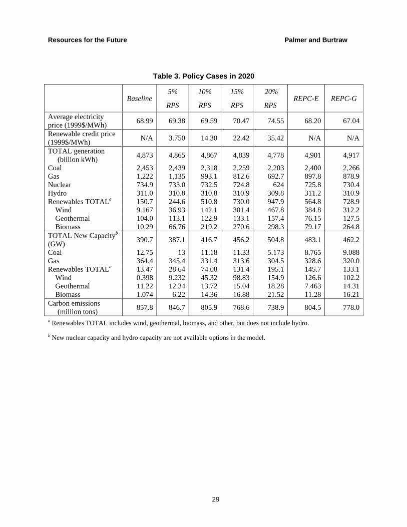
Table 3 summarizes the results for 2020 of four RPS targets: 5%, 10%, 15%, and 20%.14 The results appear consistent with prior expectations in several respects:

• The price of electricity and the renewable credit increase with the level of the RPS.

• Generation from both coal and natural gas declines as the level of the RPS increases.

• Gas generation is more dramatically affected than coal generation because it competes at the extensive margin for a share of new capacity.

• The level of carbon emissions decreases with the level of the RPS.

Although the 5% RPS policy more than doubles the level of investment in new renewables relative to the baseline in 2020, it has very little effect on electricity price, total generation, and total carbon emissions from the electricity sector. Electricity price rises by less than 1%, and total generation drops only slightly. Generation by gas units declines by 7%, but coal generation drops by less than 1%, contributing to the small magnitude of the change in carbon emissions.

The RPS credit price for a 5% RPS is roughly an order of magnitude smaller than the RPS credit price for a 20% RPS. This is understandable because the 5% RPS represents an increase of only 2 percentage points in renewable generation over the baseline level, which is about 3.1% in 2020. For the 5% and 10% RPS policies, the electricity price impact is very small, and even at the 15% RPS policy, electricity price increases by only 2.1%. However, with a 20%

14 Note that the nonhydro renewables penetration levels that result from the different RPS runs differ slightly from the minimum portfolio standards because of imperfect model convergence. For example, the model produces 4.9% renewables penetration in 2020 for the 5% RPS scenario, 10.4% for the 10% RPS, 15.08% for the 15% RPS, and 19.8% for the 20% RPS scenario.

10


RPS, electricity price in 2020 is 8.5% higher than under the baseline. The reason for this nonlinear response in price is explained below.

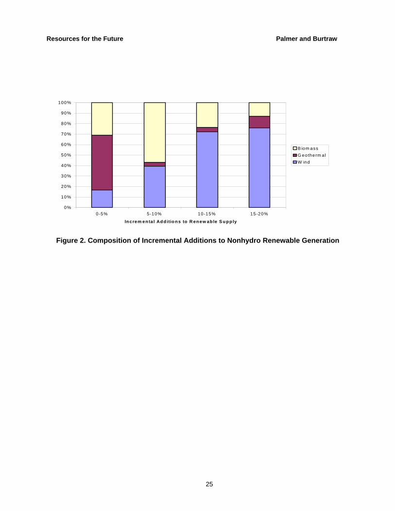
The relative importance of different classes of renewables in satisfying the RPS depends upon the stringency of the RPS. Figure 2 shows the composition of the renewable generation used to meet each 5% increment in the RPS in 2020. At the 5% RPS, as in the baseline, geothermal continues to provide the primary source of nonhydro renewable supply, although there is an important expansion in biomass generation between the baseline and the 5% level. Biomass is the most important renewable technology in the incremental generation required to go from a 5% RPS to a 10% RPS, followed by wind, with only a small expansion for geothermal. In the last two steps, from 10% to 15% and from 15% to 20%, wind is the most important contributor, accounting for more than 70% of incremental generation in each of the two steps.

With a 20% RPS, the composition of generation changes significantly as the increased use of renewables backs out generation from other sources. It has important implications for the market price of natural gas and carbon emissions. Over the decade between 2010 and 2020, the 20% RPS produces an average decline in total gas-fired electricity generation of 30% relative to the baseline, with a price of gas delivered to utilities that is 6% below baseline levels. Gas generation is 43% lower in 2020 with a 20% RPS than in the baseline scenario, and coal generation is only about 10% lower than the baseline. In relative terms, the reduction in gas generation is 210% that of coal generation. This drop in gas demand from electricity generators and the associated drop in price mean lower gas prices for residential and industrial gas consumers as well, an important political consideration.

At lower levels of the RPS, renewables displace fossil fuel generation almost exclusively. A striking finding is that at the 20% level, renewables also start to back out nuclear generation, which is roughly 15% less than in the baseline scenario, resulting in the retirement of more than half of the inefficient nuclear capacity nationwide by 2020 relative to the baseline.15 In addition, in the baseline scenario many of these existing nuclear plants make investments, known as uprates, to increase their capacity ratings. With the 20% RPS, fewer of these investments take place, which contributes to the lower level of nuclear generation.

The backing out of baseload nuclear generation in the increment between the 15% RPS and the 20% RPS—instead of backing out as much natural gas as occurred at lower levels of the RPS policies—explains why the electricity price increase is greater between the 15% RPS and 20% RPS than at other increments. Natural gas is often at the margin in electricity generation.

15 The model divides nuclear capacity into efficient and inefficient nuclear model plants in each of the 13 regions, with roughly 16% of national nuclear capacity falling in the inefficient category.

11


When gas generation is decreased, natural gas prices decrease, thereby lowering marginal generation costs of gas.

At levels of the RPS below 15%, the reduction in marginal generation costs from natural gas helps offset the cost of the RPS policy, but it was less likely to occur in the increment between the 15% RPS and the 20% RPS policies because of backing out of nuclear. In Table 3, the renewable credit price is 58% greater in the 20% RPS than in the 15% RPS policy. However, the relative change in electricity price is nearly four times as large under the 20% RPS.

The carbon emissions reductions associated with these scenarios follow from the reduction in total generation and the change in the generation mix. For the 5% and 10% RPS policies, annual carbon emissions are lower by 1.2% and 5.8%, respectively. (Recall that in the baseline, renewables already constitute 3.1% of total generation in 2020.) A 15% RPS results in carbon emissions that are 10% lower, and a 20% RPS results in carbon emissions that are 13% lower.

Prior Studies

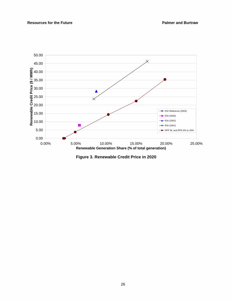
Several studies have examined how the electricity sector would respond to the imposition of an RPS (Palmer et al. 2002, Clemmer et al. 1999, Bernow et al. 1997), including a series of recent studies by U.S. EIA. Figure 3 compares the renewable credit price and the renewable generation share for our results with the EIA studies. We predict lower renewable credit prices for achieving a given level of renewable penetration than did the earlier EIA studies. Many factors contribute to these differences, including the natural gas price trajectory found in our baseline scenario, which is based on Annual Energy Outlook 2003 and is higher than the gas price forecasts underlying the other analyses, which produce lower opportunity cost of generating electricity from renewables. Our model also includes more up-to-date information about technology costs as well as updated assumptions about technological learning, both of which would tend to lower the costs of the RPS relative to earlier studies. An offsetting factor is that EIA studies include noncommercial cogenerating units that use renewable technologies and in some scenarios are allowed to earn renewable credits, contributing as much as 20% of the total nonhydro renewable generation.16

16 Another offsetting factor is that landfill gas units are not eligible to earn renewables credits in the scenarios we run. We did a sensitivity case for the 15% RPS that included landfill gas units under the RPS. For that scenario, we find that the renewables credit price is about 10% lower in 2020 when landfill gas units are included. Generation by landfill gas generators is about 30% higher, but landfill gas still accounts for only 4.5% of total nonhydro renewable generation, versus 3.4% when landfill gas units do not receive credits.

12


Figure 4 shows that the carbon intensity of generation in our model is generally higher than in the earlier EIA studies. This follows in part from the higher gas prices and greater reliance on coal-fired generation in our model than in the EIA model.

The main policy assumptions and some of the results from EIA are summarized and compared with our results in Table 4. The difference between “RPS in 2020” and “Renewable penetration” in the EIA models reflects the inclusion of firms generating electricity primarily for their own consumption, and in some cases the roles of the price cap and the sunset provision. One significant variation across these models is the change in electricity price for a given level of renewable penetration. EIA (2002b) achieves 11.7% penetration with an increase of 3% in electricity price, whereas we obtain 10% penetration with an increase in price of less than 1%. In the most recent EIA model (2003), the price increase for a 6.1% penetration is 0. There also is a substantial difference in the predicted change in natural gas prices, which ranges from negligible for 10% penetration of renewables, to a decline of 17.7% for a 16.7% penetration (EIA 2001). In general, the change in the RFF Haiku model is less than in the EIA models.

Welfare Effects of RPSs

The economic cost of the RPS and REPC policies within the electricity sector can be measured by the change in consumer and producer surplus within the sector and by the size of government revenues relative to the no-policy baseline. The REPC subsidy represents a cost because the subsidy revenue is not available to the government to spend on other government programs.17 Of course, economic surplus within the electricity sector does not account for effects outside the sector or environmental benefits from renewable generation.18

Table 5 provides a snapshot of the economic surplus changes from the baseline associated with the different RPS policies in 2020. Consumers always lose with an RPS (not accounting for environmental benefits) because in these scenarios, the RPS raises electricity price. A 5% RPS leads to an increase in producer surplus. As the RPS becomes more stringent, losses to both consumers and producers increase up to the 15% RPS policy. The total economic surplus loss under the 15% RPS is $11.27 billion, or roughly 3% of the estimated $326 billion in total electricity-sector revenue under the baseline scenario in 2020. Between the 15% RPS and the 20% RPS policies, the electricity price increase is substantial, resulting in a big drop in

17 In this analysis, we assume that $1 of government subsidy is worth $1. If we were to account for the distortions created by typical government fund-raising activities, the cost of the subsidy would be higher. Typically, the marginal cost of raising $1 in public revenue is estimated at about $1.3. 18 For a recent analysis of the benefits of reducing atmospheric emissions from electricity generation, see Banzhaf et al. (2004).

13


consumer surplus. For producers, the price increase means that they experience a smaller drop in producer surplus under the 20% RPS than under less stringent policies.

The bottom two rows of Table 5 provide information on incremental social cost, a proxy for marginal social cost, measured along two dimensions. The first is the incremental cost of increased renewable generation from the last policy. The incremental cost per megawatt-hour of increasing renewable penetration from the baseline level of 3.1% to 5% calculated as the total surplus cost of the 5% RPS divided by the additional renewable generation induced by the policy. The next column reports the incremental cost of the incremental renewable generation resulting from going from a 5% to a 10% RPS, and so on. This incremental social cost measure shows a “knee” of the curve in the incremental costs of supplying increased renewable penetration between a 15% and 20% RPS, the point at which social cost as well as electricity price (see Table 3) rise substantially. The bottom row reports incremental costs from the perspective of incremental reductions in carbon emissions. Another knee of the curve appears: incremental cost of carbon reductions is much higher for a 20% RPS than for a lesser target.

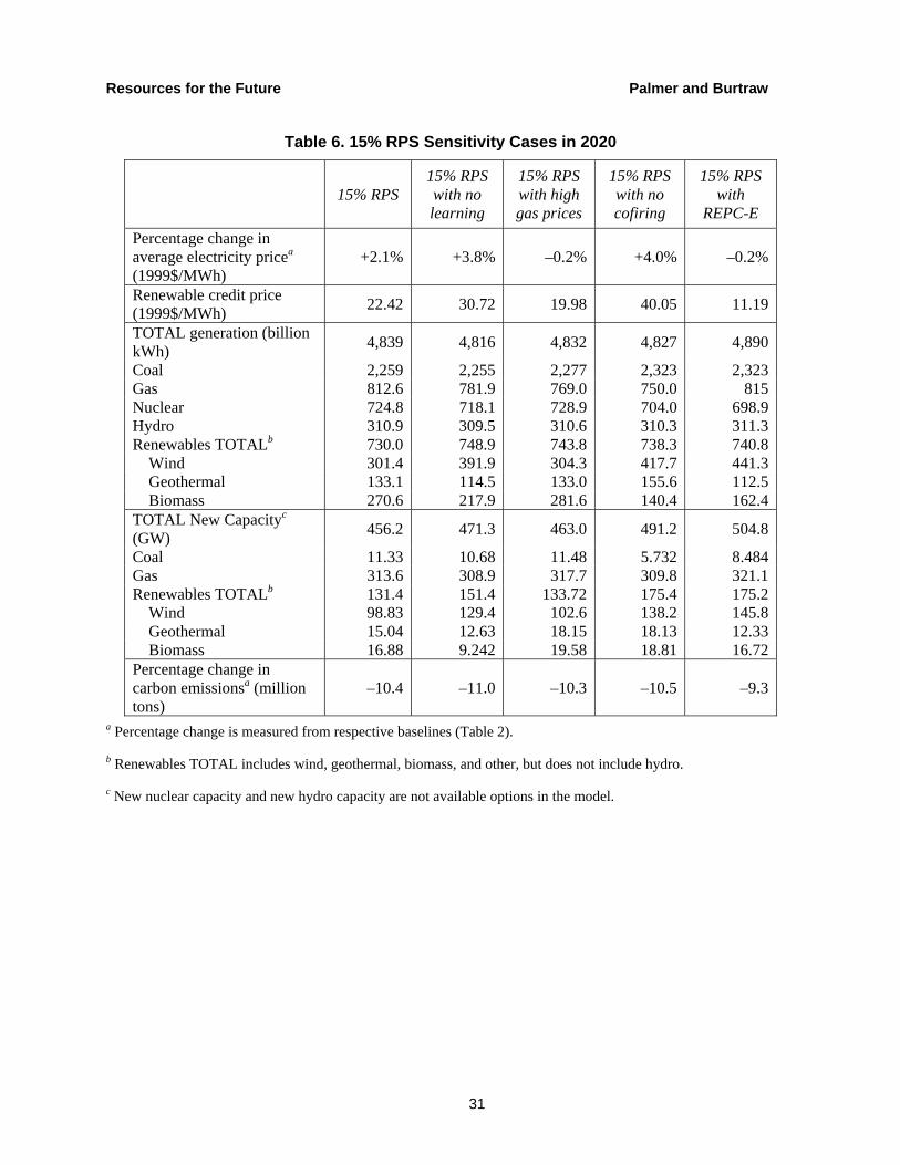
Sensitivity Analysis for the 15% RPS

Learning has become an important justification for policies to promote renewable technologies. In his seminal paper, Arrow (1962) shows that if the productivity of capital is an increasing function of the level of cumulative investment because of learning, then individual firms will underinvest in capital because they do not internalize the larger social gains from learning. From the cost perspective, the theory of learning by doing suggests that technology costs will fall as experience with a technology grows.

Learning functions typically express the cost of a technology as a constant elasticity function of the amount of accumulated capacity (Loschel 2002), where the elasticity is often referred to as the learning index. Most renewable technologies, with the possible exception of wind power, are relatively immature, and thus the potential for learning with greater market penetration is relatively high. Empirical studies suggest there is a large variation in the rate of learning across different energy technologies, with more mature technologies having substantially lower learning rates (McDonald and Schrattenholzer 2001, IEA 2000). The inappropriability of the gains from learning means that there may be a market failure at work that justifies policies to promote renewables, in addition to the usual environmental justification.

We find technological learning has a direct effect on the capital cost of a new generator and that effect can be large for new technologies like biomass integrated gasification combined cycle. The construction cost of new biomass capacity in 2020 in the 15% RPS case ($82/MW) is about 60% lower than in the 15% RPS with capital cost learning assumed not to occur. The change in cost due to learning is smaller for wind, which is characterized as a relatively more mature technology than biomass. The capital cost of wind in 2020 in the 15% RPS case is

14


$229/MW, about 21% lower than if capital cost learning is assumed not to occur. This comparison does not solely reflect learning because wind technology has an upward-sloping capacity supply function in the model, reflecting the higher capital costs associated with accessing wind resources that are of lower quality, in remote locations, or on difficult terrain. Thus, capital costs will increase as the lower-cost wind sites are used up. Table 6 indicates that when learning is turned off in the model, wind becomes more appealing relative to other renewable technologies and takes market share away from biomass, thus causing construction costs of wind to increase even more. The price of a renewable energy credit in 2020 is nearly 36% higher, and the percentage change in electricity price measured relative to the corresponding baseline (Table 2) is 3.8%, compared with 2.1% in the central case.

Another important variable is natural gas price. In the high gas price scenario, renewable credits are 11% less expensive than in the central case because the increased opportunity cost of using natural gas to generate electricity makes renewables more appealing. In another sensitivity analysis not reported in the table, we substituted the lower Annual Energy Outlook 2001 fossil fuel price assumptions for those used in the central cases and found the renewable credit price was roughly 14% higher than in the central case. Hence, we see a pattern: as the price of natural gas increases, the renewable credit price falls, and consequently the social opportunity cost of achieving greater renewable penetration in the market falls as well.

The average price of electricity in 2020 actually declines in the high gas price scenario relative to the high gas price baseline. The fall in price does not imply that the policy does not have resource costs, only that those costs are not borne by consumers. How electricity price can fall with an RPS was illustrated in Figure 1 for the central case natural gas prices for the summer baseload timeblock in the MAPP regional market. Because of their low variable cost, as renewables enter the dispatch supply curve, they push technologies with higher variable costs further down the dispatch schedule. The competitive price in the wholesale power market will be unambiguously lower in this example because the entire variable cost curve lies below the baseline. In the high gas price case, the displacement of marginal gas generation has an even greater effect.

We also examine a case in which biomass cofiring is not allowed in the baseline and does not receive credits when there is an RPS. The renewable credit price in 2020 is $40/MWh, almost twice as high as in the central case. With no cofiring, the composition of renewable generation involves substantially less biomass, more generation from wind, and somewhat more from geothermal, with an electricity price that is 2% higher than in the 15% RPS central case.

15


The last sensitivity case combines the 15% RPS with the extension of the renewable production tax credit for wind and dedicated closed-loop biomass (REPC-E). In this case, the renewable credit price is very low, reflecting the fact that the REPC-E by itself yields more than 11% renewable generation in 2020.19 The price of electricity is lower than the central case baseline for 2020. Wind achieves its largest share of total nonhydro renewable generation, and renewables start to back out nuclear generation in addition to natural gas and coal, although coal generation is higher in this scenario than in any of the other 15% RPS runs.

The last row of Table 6 indicates that, with the exception of the combination 15% RPS/REPC-E policy, the various assumptions used in the sensitivity analysis have very little effect on the level of total carbon emissions from the electricity sector in 2020. Carbon emissions are higher in the combination case, which is consistent with the higher level of total generation and with the greater reliance on coal.

7. Results for REPC

In the baseline scenarios and all the RPS policy scenarios, we assume that the REPC policy continues through simulation year 2005 and is phased out between 2005 and 2010.20 In the policy scenarios analyzed here, we extend the REPC across the full forecast horizon.21

In the REPC-E scenario, the tax credit is extended until 2020 and continues to apply only to wind and closed-loop biomass.22 Table 3 reports that electricity price is 1% lower than it is in the baseline. REPC-E results in a substantial increase in the amount and share of generation from nonhydro renewable sources, which rise to 11.5% of total generation from a baseline level of 3.1% in 2020. Most of the additional renewable generation is from wind and biomass, the two renewable technologies eligible for the production incentive. Wind generation increases by more than 380 billion kWh, to four times its level in the baseline, and biomass generation grows to more than 15 times its level in the baseline with the addition of 150 billion kWh. Generation from geothermal plants is 30 billion kWh, or 30%, lower with the REPC than in the baseline, in large part because geothermal plants do not benefit from the production incentive.

19 Note that because of imperfect convergence in the model, this model run actually yields 15.2% renewables in 2020. The actual credit price necessary to achieve 15% renewables could in fact be lower than $9.00/MWh. 20 Furthermore, we assume that facilities can earn the credit only as long as it is available to new qualified facilities. The actual provision makes the credit available for only 10 years. 21 We assume that the REPC is in effect throughout the operating life of the renewable facility. 22 The production credit is set at its historic level of 1.8 cents/kWh (in real terms) throughout the forecast period.

16


As with the low and midlevel RPS policies, in the REPC-E scenario the increased generation from renewables backs out fossil generation. As a result, gas-fired generation is roughly 26% lower than in the baseline and coal generation is lower by roughly 2%. Extending the production tax credit through 2020 reduces carbon emissions in 2020 by 53 tons or 6.2%.

To be able to compare the efficacy of a production tax credit such as the REPC with an RPS policy, we also look at a more general production tax credit, the REPC-G, targeting technologies that qualify for the RPS. The policy is constructed by translating the after-tax subsidy received by renewable generators (the renewable credit price) associated with the 15% RPS into an equivalent production tax credit. In the case of the RPS, renewables are subsidized and the funds for that subsidy effectively come from a tax on fossil fuel, nuclear, and hydro generation. In the case of the REPC-G policy, renewables receive an identical after-tax subsidy that comes from federal taxpayers.

The results for the REPC-G scenario are presented in the last column of Table 3. By design, the REPC-G policy achieves a quantity of total renewable generation in 2020 (729 GWh) comparable to the 15% RPS policy (730 GWh), although the relative shares of different technologies within that total vary somewhat. Because renewable generation is subsidized using general tax revenues, electricity price is lower and total generation is higher than in the baseline or any of the other policy scenarios. Total gas generation is 8% higher than under the 15% RPS case, and gas accounts for the lion’s share of the difference in total generation and carbon emissions between the REPC-G case and the 15% RPS case.

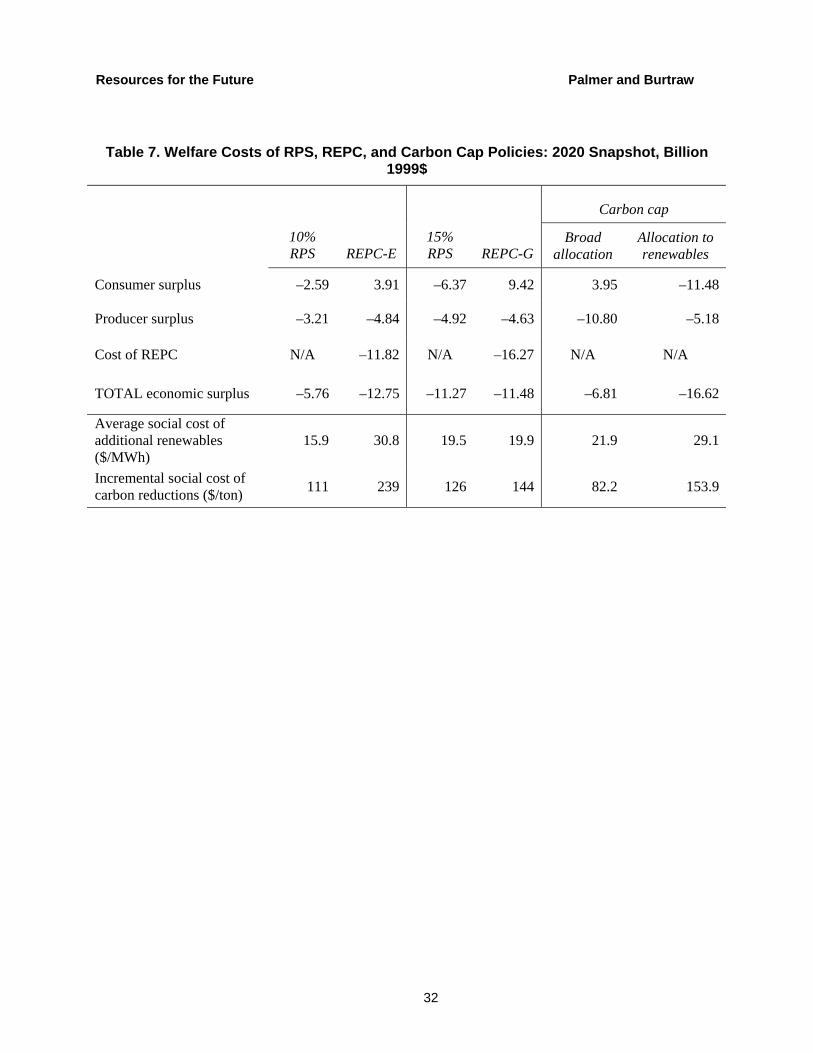
Comparing Welfare Effects of RPS and REPC Policies

Table 7 summarizes the costs of the two REPC policies and contrasts them with the RPS policy that comes closest in terms of renewable share of total generation. Thus, the 10% RPS and the REPC-E, which achieves an 11.5% renewable share, are reported together. Because the REPC-E policy (extended until 2020 but limited to wind and dedicated closed-loop biomass) yields a lower price of electricity, it makes consumers better off than they are in the baseline scenario in 2020. The loss to producers offsets the gain to consumers, but the main cost of the policy is the large size ($11.8 billion) of the subsidy to renewables associated with the cost to government. The combined effect is a $12.8 billion drop in economic surplus.

The REPC-G policy, which is expanded to a broader set of renewable technologies, is compared with the 15% RPS, since both are designed to yield a 15% renewable share. REPC-G yields the highest level of consumer surplus increases due to the low electricity price, but it also yields the highest cost to government in funding the subsidy. The REPC-G policy is less costly overall in terms of total economic surplus loss than the REPC-E because the REPC-G allows for an expanded set of options that qualify for delivering a comparable amount of renewable energy. However, the REPC-G policy is roughly 2% more costly than the 15% RPS.

17


The economic surplus consequences of regulations that raise electricity prices, such as an RPS for the electricity sector, are complicated by the fact that electricity is not priced efficiently. Often—during peak demand periods, for example—the price paid by consumers is substantially below marginal cost. This is even more likely to be the case in regions where electricity price is set using cost-of-service regulation, as assumed for much of the country in these model runs. In such cases, any policy that raises the price of electricity and thereby narrows the gap between electricity price and marginal cost leads to less of an efficiency loss than occurs with a comparable REPC policy that doesn’t raise the electricity price.

Comparing approaches, we find that the REPC-E has a greater economic cost than the 15% RPS even though it yields only an 11.5% share of generation by renewables. The REPC-G yields about the same renewable generation but is still slightly more costly than the 15% RPS. In addition, the REPC-G yields a slightly higher level of carbon emissions than the 15% RPS policy, because the subsidy provided by government helps keep electricity prices low, leading to 3% more total generation. The bottom two rows of Table 7 provide estimates of the average cost of using the two types of policies to increase renewables and to reduce carbon emissions, respectively. We find that the RPS dominates the REPC, both as a policy to promote renewables and as a policy to reduce carbon emissions.

8. Carbon Cap with Allowance Allocation on the Basis of Generation

The third policy we address is a cap-and-trade policy for CO2. One variation distributes emissions allowances to all facilities, excluding hydro and nuclear, on the basis of their share of electricity generation; this is referred to as “broad-based updating.” A second variation distributes allowances to renewable generators only based on their share of total renewable generation, called “updating to renewables.” The carbon cap is set at the level achieved under a 15% RPS.

Table 7 indicates that the carbon cap combined with a broad-based updating allocation is a more cost-effective way to reduce carbon emissions than any of the renewable policies. The average cost per ton reduced is $82 under the carbon cap versus $126 under the 15% RPS policy that achieves comparable reductions. We emphasize that the finding hinges on the way in which carbon emissions allowances are allocated. Burtraw et al. (2001) find that an updating approach to distributing carbon emissions allowances is generally two to three times more expensive than an emissions cap-and-trade program with allowances allocated by auction.

Fischer and Newell (2004) also compare the partial equilibrium social cost of different policies, using a simple economic model of electricity markets that includes a choice between two electricity-generating technologies and endogenous decisions about R&D investment by electricity generators. They find that an RPS set to achieve a 5.8% reduction in carbon emissions is 7.5 times as costly in terms of social welfare as using an emissions tax (equivalent to a cap-

18


and-trade policy with allowances distributed by auction) to achieve the same emissions reduction.

In summary, we find the RPS policies to be more cost-effective in achieving renewable penetration in the market than a carbon cap coupled with updating allocation of emissions allowances. The carbon cap combined with a broad-based updating performs fairly well in boosting renewables, but a carbon cap with updating to renewables is much more expensive. However, if the primary goal of policy is to reduce carbon emissions, then a carbon cap with broad-based allowance distribution is the more cost-effective policy.

9. Conclusions

This study evaluates different approaches to supporting renewable generation in the U.S. electricity sector and their effects on emissions of greenhouse gases. We find the social cost of RPS policies to be somewhat less than suggested by previous studies when cost is measured as the magnitude of the RPS credit or as the change in electricity price. Several factors contribute to this result, including newer forecasts of higher natural gas prices into the future and updated information on technology cost and performance of renewables.

The RPS raises electricity prices, lowers total generation, reduces gas-fired generation primarily, and lowers carbon emissions, with the size of these effects growing with the stringency of the portfolio standard. At lower levels (5%–10%), the RPS is met largely by geothermal and biomass, which leads to increased generation in the West (geothermal) and in regions where biomass has an economic advantage over other renewable sources. At higher (10%–20%) RPS levels, wind generation becomes a major component of the incremental renewable generation required to meet the standard.

A knee to the cost curve for RPS targets appears between 15% and 20% targets for 2020. In our central case and with targets up to 15%, the change in electricity price is modest, but the change in price for a 20% target is substantially greater. Also, the cost of reducing carbon emissions is greater at a 20% renewable target because some of the incremental penetration of renewables is achieved with reduced nuclear generation, which has no carbon emissions.

We find that the cost of achieving increased renewable generation is inversely related to natural gas prices. In the high gas price scenario, which is tailored to Annual Energy Outlook 2004 price forecasts, electricity price actually falls relative to the corresponding baseline in achieving a 15% target.

The RPS policy appears to be more cost-effective than either REPC policy in both promoting renewables and reducing carbon. Extending the REPC policy that benefits only wind and dedicated closed-loop biomass through 2020—the REPC-E scenario—produces a large increase in renewable generation, pushing the total share of nonhydro renewables above 11% in

19


2020. However, this policy also produces a lower electricity price, which limits its effectiveness in reducing carbon emissions. In addition, the total economic surplus cost of the REPC-E is greater than that of a 15% RPS policy, which does a better job of accomplishing these goals without imposing costs on federal taxpayers. Combining an REPC-E with an RPS appears to be ill advised, given that introducing the subsidy raises efficiency costs and total carbon emissions, the latter of which is due in part to the higher level of electricity production.

The REPC policy aimed at a general portfolio of renewable technologies—the REPC-G scenario—is more cost-effective than REPC-E. When designed to achieve the same quantity of total renewable generation as the 15% RPS, however, it does so at greater social cost and with a smaller reduction in carbon emissions. On net, we find the RPS approach to be superior to the REPC approach. One remaining justification for an REPC is its potential value as a policy instrument in supporting new and immature technologies. Similarly, an RPS could set targets for specific types of technology. In either case, such a precise design with respect to a narrow qualifying technology is beyond this analysis.

We find that the RPS can produce important reductions in carbon emissions as a result of both higher electricity prices and shifts away from fossil fuel generation to renewables. However, these emissions reductions are not as large as they would be if renewable generation were displacing coal instead of natural gas. Moreover, the emissions reductions are tempered by the tendency for renewables to start to back out existing nuclear generation at higher levels of the RPS. All of these factors contribute to making the RPS less effective in absolute terms and less cost-effective as a mechanism for reducing carbon emissions from electricity generators than a policy designed specifically to limit carbon emissions.

In conclusion, the RPS policy appears to be superior for promoting renewables and reasonably effective at achieving direct reductions in carbon emissions, although not as effective as a carbon cap policy. Moreover, substantial renewable penetration of 15% by 2020 can be achieved at a modest cost for consumers and a modest economic cost, and that cost decreases as natural gas prices rise. Renewable penetration beyond 15% by 2020 appears to be substantially more expensive.

20


References

Arrow, Kenneth. 1962. The Economic Implications of Learning-by-Doing. Review of Economic Studies 29: 155–73.

Banzhaf, Spencer, Dallas Burtraw, and Karen Palmer. 2004. Efficient Emissions Fees in the U.S. Electricity Sector. Resource and Energy Economics 26(3): 317–41.

Bernow, Stephen, William Dougherty, and Mark Duckworth. 1997. Quantifying the Impacts of a National, Tradable Renewables Portfolio Standard. The Electricity Journal 10(4): 42–52.

Bolinger, Mark, and Ryan Wiser. 2003. Comparison of AEO 2004 Natural Gas Price Forecast to NYMEX Futures Prices. Berkeley, CA: Lawrence Berkeley National Laboratory. December 19.

Burtraw, Dallas, Karen Palmer, Ranjit Bharvirkar, and Anthony Paul. 2001. The Effect of Allowance Allocation on the Cost of Carbon Emissions Trading. Discussion Paper 01-30. Washington, DC: Resources for the Future. August.

Clemmer, Steve, Alan Nogee, and Mark Brower. 1999. A Powerful Opportunity: Making Renewable Electricity the Standard. Cambridge, MA: Union of Concerned Scientists. January.

Darmstadter, Joel. 2003. The Economic and Policy Setting of Renewable Energy: Where Do Things Stand? Discussion Paper 03-64. Washington, DC: Resources for the Future. December.

EIA (U.S. Energy Information Administration). 2001. Analysis of Strategies for Reducing Multiple Emissions from Electric Power Plants: Sulfur Dioxide, Nitrogen Oxides, Carbon Dioxide, and Mercury and a Renewable Portfolio Standard, SR/OIAF/2001–03. Washington, DC: Department of Energy. July.

———. 2002a. Annual Energy Outlook 2003. DOE/EIA-0383 (2003). Washington, DC: Department of Energy. December.

———. 2002b. Impacts of a 10-Pecrent Renewable Portfolio Standard. SR/OIAF/2002–03, Washington, DC: Department of Energy. February.

———. 2003. Analysis of a 10-Percent Renewable Portfolio Standard. SR/OIAF/2003–01, Washington, DC: Department of Energy. May.

21


———. 2004. Annual Energy Outlook 2004, DOE/EIA-0383 (2004). Washington, DC: Department of Energy. January.

Energy Modeling Forum. 1998. A Competitive Electricity Industry. Final report of EMF Working Group 15. Stanford, CA: Stanford University.

———. 2001. Prices and Emissions in a Restructured Electricity Market. Final report of EMF Working Group 17. Stanford, CA: Stanford University.

Energy Research Centre of the Netherlands. 2004. Renewable Energy Fact Sheets: EU Countries. Available from http://www.renewable-energy-policy.info/relec/index.html (accessed September 20, 2004).

ESD (Energy for Sustainable Development Ltd.). 2001. The European Renewable Energy Certificate Trading Project. Research report funded by the European Commission. Overmoor, Neston, Wiltshire, U.K.: ESD. September.

Fischer, Carolyn, and Richard Newell. 2004. Environmental and Technology Policies for Climate Change and Renewable Energy. Discussion Paper 04-05. Washington, DC: Resources for the Future. April.

IEA (International Energy Agency). 2000. Experience Curves for Energy Technology Policy. Paris: IEA.

Keiko, Omori. 2003. Switching On to New Energy Sources. Look Japan September 1: 26–27.

Lagniss, Ole, and Ryan Wiser. 2003. The Renewables Portfolio Standard in Texas: An Early Assessment. Energy Policy 31(6): 527–35.

Loschel, Andreas. 2002. Technological Change in Economic Models of Environmental Policy: A Survey. Ecological Economics 43: 105–26.

McDonald, A., and Leo Schrattenholzer. 2001. Learning Rates for Energy Technologies. Energy Policy 29: 255–61.

McVeigh, James, Dallas Burtraw, Joel Darmstadter, and Karen Palmer. 2000. Winner, Loser, or Innocent Victim: Has Renewable Energy Performed as Expected? Solar Energy 68(3): 237–55.

Palmer, Karen, and Dallas Burtraw. 2004. Electricity, Renewables, and Climate Change: Searching for a Cost-Effective Policy. Report. Washington, DC: Resources for the Future. May.

22

http://www.renewable-energy-policy.info/relec/index.html


Palmer, Karen, Dallas Burtraw, Ranjit Bharvirkar, and Anthony Paul. 2002. Electricity Restructuring, Environmental Policy, and Emissions. Report. Washington, DC: Resources for the Future. December.

Quené, Marjolein. 2002. Aim of the Day for RECS. Opening speech of the RECS Open Seminar, E.U. Symposium, Pisa, Italy. September 27.

Sterner, Thomas, and Lena Hoglund. 2000. Output-Based Refunding of Emissions Payments: Theory, Distribution of Costs, and International Experience. Discussion Paper 00-29. Washington, DC: Resources for the Future. June.

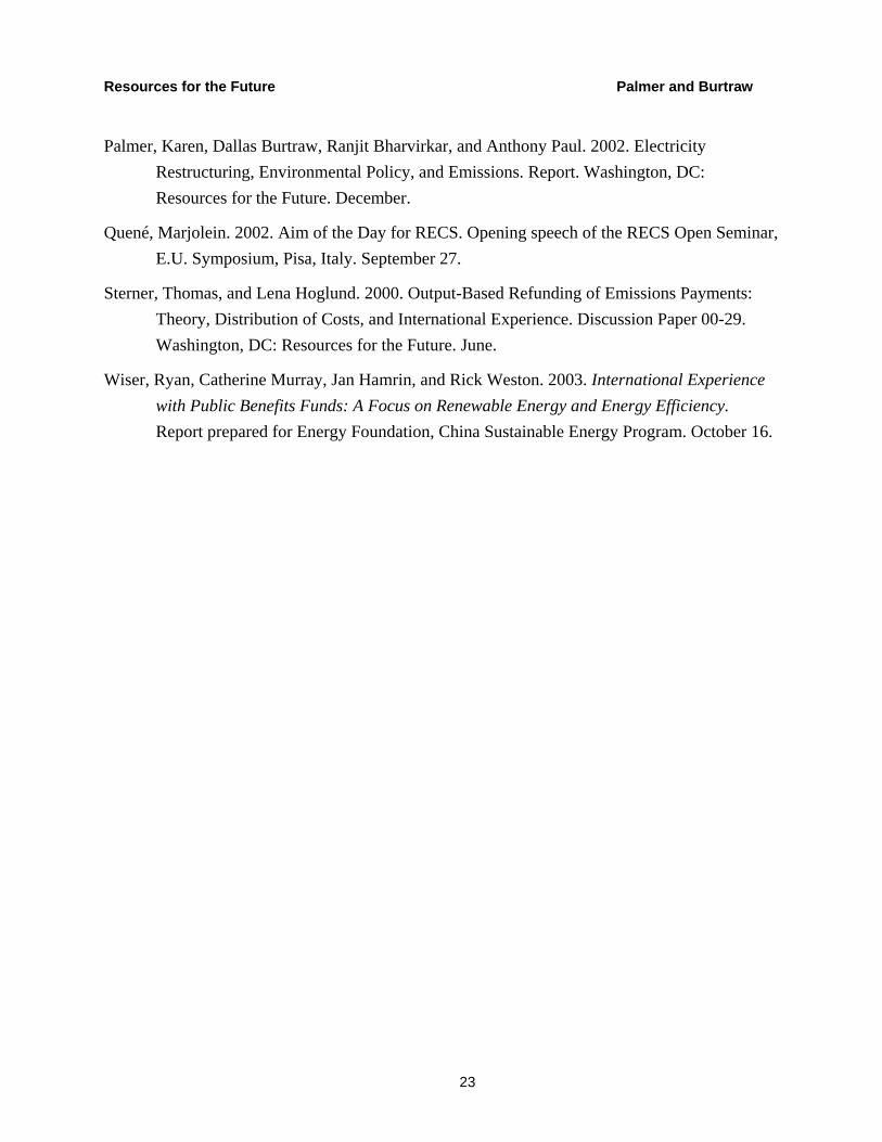
Wiser, Ryan, Catherine Murray, Jan Hamrin, and Rick Weston. 2003. International Experience with Public Benefits Funds: A Focus on Renewable Energy and Energy Efficiency. Report prepared for Energy Foundation, China Sustainable Energy Program. October 16.

23


Figures

MAPP Summer Peak

-40

-20

0

20

40

60

80

100

120

0 5 10 15 20 25 30 35 40 45

Capacity (GW)

Mar

gina

l Cos

t ($/

MW

h)

BaselineBL Plants15% RPS15% RPS Plants

Avg Unscrubbed Coal

New Biomass

New Gas CC

Existing Efficient Gas Turbine

Figure 1. Effect of RPS on System Dispatch

24


0%

10%

20%

30%

40%

50%

60%

70%

80%

90%

100%

0-5% 5-10% 10-15% 15-20%

In crem en ta l Ad d itio n s to R en ew ab le S u p p ly

B iom assG eotherm a lW ind

Figure 2. Composition of Incremental Additions to Nonhydro Renewable Generation

25


0.00

5.00

10.00

15.00

20.00

25.00

30.00

35.00

40.00

45.00

50.00

0.00% 5.00% 10.00% 15.00% 20.00% 25.00%Renewable Generation Share (% of total generation)

Ren

ewab

le C

redi

t Pric

e ($

/ M

Wh)

EIA Reference (2003)

EIA (2003)

EIA (2002)

EIA (2001)

RFF BL and RPS 5% to 20%

Figure 3. Renewable Credit Price in 2020

26


0

0.02

0.04

0.06

0.08

0.1

0.12

0.14

0.16

0.18

0.00% 5.00% 10.00% 15.00% 20.00% 25.00%Renewable Generation Share (% of total generation)

Car

bon

Inte

nsity

(met

ric to

ns /

MW

h)

EIA Reference (2003)

EIA (2003)

EIA (2002)

EIA (2001)

RFF BL and RPS 5% to 20%

Figure 4. Carbon Intensity of Electricity Generation in 2020

27


Tables

Table 1. Phase-in of Renewable Portfolio Standard Targets

Minimum renewable requirement by year RPS target for 2020

2005 2010 2015 2020 5% 1.25% 2.5% 3.75% 5%

10% 2.5% 5.0% 7.5% 10% 15% 2.5% 6.5% 10.5% 15% 20% 2.5% 8.0% 14.0% 20%

Table 2. Baseline Cases in 2020

Central case baseline

Baseline with no learning

Baseline with high gas prices

Baseline with no cofiring

Average electricity price (1999$/MWh) 68.99 69.96 71.27 69.22

TOTAL generation (billion kWh) 4,873 4,861 4,842 4,872 Coal 2,453 2,445 2,499 2,459 Gas 1,222 1,263 1,100 1,219 Nuclear 734.9 730.9 739.7 733.1 Hydro 311.0 310.9 310.9 310.9 Renewables TOTALa 150.7 110.0 204.3 144.4 Wind 9.167 9.851 11.19 9.018 Geothermal 104.0 67.85 106.7 97.16 Biomass 10.29 4.329 39.41 13.81 TOTAL new capacityb (GW) 390.7 380.7 388.1 385.5 Coal 12.75 11.49 18.43 13.65 Gas 364.4 360.9 350.8 358.7 Renewables TOTALa 13.47 8.254 18.73 12.63 Wind 0.398 0.841 1.249 0.300 Geothermal 11.22 6.442 11.52 10.43 Biomass 1.074 0.095 4.948 1.518 Carbon emissions (million tons) 857.8 860.6 856.3 858.7

a Renewables TOTAL includes wind, geothermal, biomass, and other but does not include hydro.

b New nuclear capacity and hydro capacity are not available options in the model.

28


Table 3. Policy Cases in 2020

Baseline

5%

RPS

10%

RPS

15%

RPS

20%

RPS REPC-E REPC-G

Average electricity price (1999$/MWh) 68.99 69.38 69.59 70.47 74.55 68.20 67.04

Renewable credit price (1999$/MWh) N/A 3.750 14.30 22.42 35.42 N/A N/A

TOTAL generation (billion kWh) 4,873 4,865 4,867 4,839 4,778 4,901 4,917

Coal 2,453 2,439 2,318 2,259 2,203 2,400 2,266Gas 1,222 1,135 993.1 812.6 692.7 897.8 878.9Nuclear 734.9 733.0 732.5 724.8 624 725.8 730.4Hydro 311.0 310.8 310.8 310.9 309.8 311.2 310.9Renewables TOTALa 150.7 244.6 510.8 730.0 947.9 564.8 728.9 Wind 9.167 36.93 142.1 301.4 467.8 384.8 312.2 Geothermal 104.0 113.1 122.9 133.1 157.4 76.15 127.5 Biomass 10.29 66.76 219.2 270.6 298.3 79.17 264.8TOTAL New Capacityb (GW) 390.7 387.1 416.7 456.2 504.8 483.1 462.2

Coal 12.75 13 11.18 11.33 5.173 8.765 9.088Gas 364.4 345.4 331.4 313.6 304.5 328.6 320.0Renewables TOTALa 13.47 28.64 74.08 131.4 195.1 145.7 133.1 Wind 0.398 9.232 45.32 98.83 154.9 126.6 102.2 Geothermal 11.22 12.34 13.72 15.04 18.28 7.463 14.31 Biomass 1.074 6.22 14.36 16.88 21.52 11.28 16.21Carbon emissions

(million tons) 857.8 846.7 805.9 768.6 738.9 804.5 778.0

a Renewables TOTAL includes wind, geothermal, biomass, and other, but does not include hydro.

b New nuclear capacity and hydro capacity are not available options in the model.

29


Table 4. Comparison of EIA RPS Studies with a 20-Year Horizon

EIA 2001 EIA 2002b EIA 2003 a RFF RPS in 2020 (%) 10 20 10 20 10 10 15 20 RPS credit price cap (cents) None 3 1.5 (nominal) None

RPS sunset date None 2020 2030 None Qualifying renewables All New New All except landfill gas

Basis for RPS All

Excludes existing renewable and

small generators

Excludes existing renewable and

small generators All

Renewable penetration in electricity grid (in model) (%)

8.2 16.7 8.4 11.7 6.1 10.4 15.1 19.8

RPS credit price (cents) 2.5 5.0 2.9 2.9 0.9 1.4 2.2 3.5

Electricity price impact (%) +<0.1 +4.2 +1.5 +3.0 0 +0.9 +2.1 +8.1

Natural gas price impact (%) –8.4 –17.7 –3.7 –6.7 –0.3 –

0.3 –0.7 – 1.0

Carbon emissions impact (electricity only) (%)

–7.2 –17.6 –6.7 –7.3 –2.8 –6.1 –10.4 –13.9

a Renewable energy production credit extended through 2006 and applied to more technologies.

Table 5. Welfare Costs of RPS Policies: 2020 Snapshot, Billion 1999$

5% RPS

10% RPS

15% RPS

20% RPS

Consumer surplus –1.93 –2.59 –6.37 –25.46

Producer surplus 1.66 –3.21 –4.92 –1.62

Cost of REPC N/A N/A N/A N/A

TOTAL economic surplusa –0.24 –5.76 –11.27 –27.08

Incremental social cost of renewables ($/MWh) 2.56 20.7 25.1 72.6

Incremental social cost of carbon reductions ($/ton) 21.6 135 148 532

aThe economic surplus measures do not include any environmental benefits resulting from the policy.

30


Table 6. 15% RPS Sensitivity Cases in 2020

15% RPS 15% RPS with no learning

15% RPS with high gas prices

15% RPS with no cofiring

15% RPS with

REPC-E Percentage change in average electricity pricea (1999$/MWh)

+2.1% +3.8% –0.2% +4.0% –0.2%

Renewable credit price (1999$/MWh) 22.42 30.72 19.98 40.05 11.19

TOTAL generation (billion kWh) 4,839 4,816 4,832 4,827 4,890

Coal 2,259 2,255 2,277 2,323 2,323Gas 812.6 781.9 769.0 750.0 815Nuclear 724.8 718.1 728.9 704.0 698.9Hydro 310.9 309.5 310.6 310.3 311.3Renewables TOTALb 730.0 748.9 743.8 738.3 740.8 Wind 301.4 391.9 304.3 417.7 441.3 Geothermal 133.1 114.5 133.0 155.6 112.5 Biomass 270.6 217.9 281.6 140.4 162.4TOTAL New Capacityc (GW) 456.2 471.3 463.0 491.2 504.8

Coal 11.33 10.68 11.48 5.732 8.484Gas 313.6 308.9 317.7 309.8 321.1Renewables TOTALb 131.4 151.4 133.72 175.4 175.2 Wind 98.83 129.4 102.6 138.2 145.8 Geothermal 15.04 12.63 18.15 18.13 12.33 Biomass 16.88 9.242 19.58 18.81 16.72Percentage change in carbon emissionsa (million tons)

–10.4 –11.0 –10.3 –10.5 –9.3

a Percentage change is measured from respective baselines (Table 2).

b Renewables TOTAL includes wind, geothermal, biomass, and other, but does not include hydro.

c New nuclear capacity and new hydro capacity are not available options in the model.

31


Table 7. Welfare Costs of RPS, REPC, and Carbon Cap Policies: 2020 Snapshot, Billion 1999$

Carbon cap

10% RPS REPC-E

15% RPS REPC-G

Broad allocation

Allocation to renewables

Consumer surplus –2.59 3.91 –6.37 9.42 3.95 –11.48

Producer surplus –3.21 –4.84 –4.92 –4.63 –10.80 –5.18

Cost of REPC N/A –11.82 N/A –16.27 N/A N/A

TOTAL economic surplus –5.76 –12.75 –11.27 –11.48 –6.81 –16.62

Average social cost of additional renewables ($/MWh)

15.9 30.8 19.5 19.9 21.9 29.1

Incremental social cost of carbon reductions ($/ton) 111 239 126 144 82.2 153.9

32

Documents

Cost-Effectiveness of Renewable Electricity Policies · Cost-Effectiveness of Renewable Electricity Policies ... renewable energy, electricity, renewable portfolio standard, ... often