Embed Size (px)
Citation preview

The Double Heston Model via Filtering
Methods
by
Elia N Namundjebo
Thesis presented in partial fullment of the requirements for
the degree of Master of Science in Financial Mathematics in
the Faculty of Science at Stellenbosch University
Supervisor: Prof. Je Sanders
Co-supervisor: Prof. Ronald Becker
December 2016

Declaration
By submitting this thesis electronically, I declare that the entirety of the workcontained therein is my own, original work, that I am the sole author thereof(save to the extent explicitly otherwise stated), that reproduction and pub-lication thereof by Stellenbosch University will not infringe any third partyrights and that I have not previously in its entirety or in part submitted it forobtaining any qualication.
December 2016Date: . . . . . . . . . . . . . . . . . . . . . . . . . . . . . . .
Copyright© 2016 Stellenbosch UniversityAll rights reserved.
i
Stellenbosch University https://scholar.sun.ac.za

Abstract
The Double Heston Model via Filtering Methods
E. N Namundjebo
Department of Mathematical Science,
Mathematics Division,
University of Stellenbosch,
Private Bag X1, Matieland 7602, South Africa.
Thesis: MSc
May 2016
Stochastic volatility models are well-known for their ability to generate avolatility smile for nancial securities. The development of the stochasticvolatility models followed shortly after the crash of 1987 which violates theBlack-Scholes model which has constant volatility. In this study we introducenon-linear ltering methods to estimate the implied volatilities of the DoubleHeston model. We compare our results to the Standard Heston model. Thenon-linear ltering methods used are the extended Kalman lter, the unscentedKalman lter and the particle lter. We combine the ltering methods togetherwith the maximum likelihood estimation method to estimate the model's hid-den parameters. Our numerical results show that the Double Heston modelts the market implied volatilities better than the Standard Heston model.The particle lter also performs better than the other two lters.
Keywords: Stochastic volatility model, Double Heston model, non-linear l-tering, maximum likelihood estimation.
JEL Classication: C11, C13, C60, G12
ii
Stellenbosch University https://scholar.sun.ac.za

Uittreksel
Die dubbel Heston Model van Filter Metodes
(Die dubbel Heston Model van Filter Metodes)
E. N Namundjebo
Departement Wiskundige Wetenskappe,
Universiteit van Stellenbosch,
Privaatsak X1, Matieland 7602, Suid Afrika.
Tesis: MSc
Mei 2016
Stogastiese wisselvalligheid modelle is goed bekend vir hul vermoë om'n wis-selvalligheid glimlag vir nansiële sekuriteite te genereer. Die ontwikkeling vandie stogastiese wisselvalligheid modelle het gevolg kort nadat die ongeluk van1987 wat die Black-Scholes model wat konstant wisselvalligheid oortree het.In hierdie studie stel ons nie-lineêre lter metodes voor om die gelmpliseerdewisselings in die Double Heston Model te skat. Ons vergelyk ons resultate aandie Standard Heston model. Die nie-lineêre lter metodes wat gebruik word isdie uitgebreide Kalman lter, die reuklose Kalman lter en die deeltjies lter.Ons kombineer die lter metodes saam met die maksimum annneemlikheidsbe-raming metode om verborge parameters van die model te skat. Ons numerieseresultate dui daarop dat die Double Heston model pas die mark gelmpliseerdevolatiliteit en beter as die Standard Heston model. Die deeltjie lter presteerook beter as die ander twee lters.
iii
Stellenbosch University https://scholar.sun.ac.za

Acknowledgements
I would like to thank my project supervisor, Prof Ronald Becker for his guid-ance and support throughout this research. Martha Kamkuemah thank youfor your valuable comments. Thanks are also due to AIMS and Namsa forfunding my studies. The hospitality of AIMS is gratefully acknowledged.
iv
Stellenbosch University https://scholar.sun.ac.za

Contents
Declaration i
Abstract ii
Uittreksel iii
Acknowledgements iv
Contents v
1 Introduction 1
2 Filtering Methods 4
2.1 Kalman Filter . . . . . . . . . . . . . . . . . . . . . . . . . . . . 62.2 Extended Kalman Filter . . . . . . . . . . . . . . . . . . . . . . 92.3 Unscented Kalman Filter . . . . . . . . . . . . . . . . . . . . . . 112.4 Maximum Likelihood Estimation(MLE) . . . . . . . . . . . . . . 142.5 Particle Filter . . . . . . . . . . . . . . . . . . . . . . . . . . . . 17
3 Stochastic Volatility Models 22
3.1 The Heston Model . . . . . . . . . . . . . . . . . . . . . . . . . 233.2 The Double Heston Model . . . . . . . . . . . . . . . . . . . . . 243.3 State-Space Representations . . . . . . . . . . . . . . . . . . . . 29
4 Empirical Analysis 35
4.1 Data . . . . . . . . . . . . . . . . . . . . . . . . . . . . . . . . . 354.2 Fitting lters . . . . . . . . . . . . . . . . . . . . . . . . . . . . 374.3 Parameters in the Heston model . . . . . . . . . . . . . . . . . . 394.4 Parameters in the Double Heston model . . . . . . . . . . . . . 42
5 Conclusion 47
A Kalman lter 49
A.1 Probability properties . . . . . . . . . . . . . . . . . . . . . . . . 49A.2 Kalman ltering . . . . . . . . . . . . . . . . . . . . . . . . . . . 50
v
Stellenbosch University https://scholar.sun.ac.za

CONTENTS vi
B MATLAB codes 56
B.1 Heston EKF . . . . . . . . . . . . . . . . . . . . . . . . . . . . . 56B.2 Heston UKF . . . . . . . . . . . . . . . . . . . . . . . . . . . . . 58B.3 Heston PF . . . . . . . . . . . . . . . . . . . . . . . . . . . . . . 61B.4 Double Heston EKF . . . . . . . . . . . . . . . . . . . . . . . . 63B.5 Double Heston UKF . . . . . . . . . . . . . . . . . . . . . . . . 66B.6 Double Heston PF . . . . . . . . . . . . . . . . . . . . . . . . . 69
List of References 71
Stellenbosch University https://scholar.sun.ac.za

Chapter 1
Introduction
Studying the implied volatility smile is important for understanding marketprices and uctuations. It has played a vital role in derivatives pricing andhedging, portfolio selection, risk management, market marking and monetarypolicy making, amongst others. A risk manager needs to know the likelihoodthat the portfolio he is holding is going to face high risk (with high volatility)in the future. An option trader will want to estimate the volatility uctua-tions of the contract until maturity. An investor would like to know his stockfuture price movements. Policymakers rely on market volatility to determinethe vulnerability of nancial markets and the economy. There is vast literaturein modelling the volatility smile. The models with a stochastic variance pro-cess known as stochastic volatility models are ecient in modelling the smile.However, implementing the stochastic volatility models remains a challenge.In this dissertation, we introduce non-linear ltering techniques for estimatingthese models as well as interpolating implied volatility term structure thatprecisely matches the market implied volatility smile.
The modelling of volatility uctuations is challenging because volatility is un-certainty. The Black-Scholes (1973) model assumes a constant volatility inthe option pricing model. The empirical literature on option pricing modelshas documented arbitrage due to the constant-volatility of the Black-Scholesoption pricing model. After the work of Hull and White (1987) and Scott(1987), the majority of option pricing models can be characterized as stochas-tic volatility models, in which the volatility of the asset returns is driven bya stochastic variance process. A stochastic volatility model of an asset is amodel of the form
dSt = rStdt+ V pt dWt
dVt = a(t, Vt)dt+ b(t, Vt)dZt
where r, p are positive constants and the subscript t is the time-step. The rstequation denes the stock price process and the second equation denes the
1
Stellenbosch University https://scholar.sun.ac.za

CHAPTER 1. INTRODUCTION 2
volatility process. The functions for volatility a and b are deterministic, andWt, Zt are mutually correlated Brownian motions.
Stochastic volatility models are widely used to model the volatility smile dueto their stochastic variance process. Common stochastic volatility models arethe SABR model, Hull and White (1987), Scott (1987), Stein and Stein (1991),and Heston (1993) models to name a few. The Heston (1993) model is the mostpopular of these option pricing models because of its closed-form expressionfor pricing options. However, according to Due et al. (2000), the Heston(1993) model fails to capture slope and level movements of the volatility smile.The empirical studies documented that the market data displays positive aswell as negative correlations, but the Heston (1993) model always yields neg-ative correlation. Christoersen et al. (2009) proposed a two-factor stochasticvolatility model, named the Double Heston model which is an extension tothe Heston (1993) model. The Double Heston model consists of an asset priceprocess driven by two uncorrelated variance processes. Empirical studies showthat the Double Heston model ts the implied volatility smile much betterthan the Standard Heston model and it displays both negative and positivecorrelations in the market data.
In this study we implement the Standard Heston and the Double Hestonstochastic volatility models and demonstrate the dierences in pricing per-formance. Typically, this will be done by comparing their implied volatilitiesterm structures. However, implementing these stochastic volatility models ischallenging. Most of the challenges arise because the volatility is not directlyobservable. It therefore needs to be extracted from observable market quotesfor example, stock prices, option prices and interest rates. The variance pro-cess consists of unknown parameters, and estimating these parameters is alsoa challenge. We therefore do the volatilities and parameters estimation usingnon-linear ltering techniques combined with the maximum likelihood estima-tion method.
The three non-linear ltering techniques in this study are the extended Kalmanlter, the unscented Kalman lter and particle lter. We use put option priceson Dow Jones Industrial Average to estimate the implied volatilities underthe Standard Heston and Double Heston models. Each of the above modelsuses ltering methods which allow us to compare the models' and lters per-formances. The ltering methods are used to estimate the models' impliedvolatilities, whereas the maximum likelihood estimation method estimates themodel's parameters. We nd that the Double Heston model captures the termstructure of the market implied volatilities better than the Standard Hestonmodel. The Heston model fails to t the data especially at shorter maturities.The extended Kalman lter performs poorly compared to the other lters. Theparticle lter under the Double Heston model ts the market implied volatili-
Stellenbosch University https://scholar.sun.ac.za

CHAPTER 1. INTRODUCTION 3
ties smile very well.
Our study contributes and relates to the active literature in modelling the im-plied volatility smile using stochastic volatility models. We are not the rst toimplement stochastic volatility models using the ltering approach, but we arethe rst to use ltering methods on the Double Heston model. Previous liter-ature implement the Standard Heston model via the ltering approach usingtime-series of underlying returns, see Javaheri et al. (2003). Li (2013) uses theltering methods on the Standard Heston model using both stock and optionprices, and claims that stock prices or option prices alone does not give goodt of the implied volatilities smile and both stock and option prices are neededfor better estimates. Guo et al. (2014) use the Nelson-Siegel term structuremodel to construct the implied volatility term structure under the Double He-ston model using S&P 500 index call options. In the yield curves modelling itis well known that the Nelson-Siegel model is empirically successful but theo-retically weak, therefore using such an approach might contribute errors in theestimated implied volatilities. Although our study relates to Rouah (2013), itdiers in the approaches used to estimate the models' volatilities as well asthe parameters. Our approach is simple to implement, with little computationburden and gives precise estimates that t the market data.
The rest of the paper is organized as follows. Chapter 2 describes the lteringmethods and presents their algorithms and the maximum likelihood estima-tion method. Chapter 3 presents the theory behind the Standard Heston andDouble Heston stochastic volatility models. We also provide the state-formrepresentations for both model. For a formal denition of the state-space rep-resentation see Section 3.3.1. The empirical evidence of the implied volatilitiesterm structures as well the estimated parameters are provided in Chapter 4.Finally, Chapter 5 concludes the paper. All the implementations have beendone in MATLAB. We developed all the codes in this study, and referencedexternal/additional functions. In the Appendices, we presents theory behindthe Kalman lter and the MATLAB codes used in this study.
Stellenbosch University https://scholar.sun.ac.za

Chapter 2
Filtering Methods
In a dynamical system with a series of past and current noisy observations,ltering is used to estimate the internal states of these systems. The system'sstates are unobservable, but observation variables are observable. Filtering isthen used to estimate the conditional probability distribution of the system'sstates given the observation variables. This is done in a two-step process. Therst step is known as the prediction step. In the prediction step, suppose thevector xk represents the current system's state at the current time k, and letthe prediction of xk at time k be xk|k−1. The state vector xk|k−1 is predictedusing past estimated states xk−1 which are assumed to be known. Filteringestimates the past states xk−1 without conditioning on previous observationsyk−1. The second step is called update step. In the update step, current statesxk|k are estimated by combining the predicted states xk|k−1 with the currentobservations yk. Since the observations are noisy, we seek the best estimatexk|k of xk that minimises the error xk − xk|k. This is done recursively at eachtime step k.
In the literature, dierent ltering methods are proposed. A Kalman lter isone of the optimal ltering methods widely used in the eld of science, engi-neering and nance. It is considered easy to understand with little computa-tional burdens. In nance it is used in estimation of risk premia, optimal assetallocation, credit risk and interest rate term structure modelling, volatilityestimation, and hedging under partial observation. The Kalman lter, how-ever, is not applicable to non-linear systems. In this chapter we discuss andpresent some of non-linear ltering methods that are applicable to non-linearsystems. We also look at the basic concepts and algorithms for these lters.These lters are the extended Kalman lter and the unscented Kalman lter.Since in general, the dynamic systems that represent the states consist of un-known parameters. Therefore, we also discuss maximum likelihood estimationmethod for estimating the parameters. Lastly, we present another lteringmethod which is slightly dierent from the Kalman ltering extensions calledthe particle lter.
4
Stellenbosch University https://scholar.sun.ac.za

CHAPTER 2. FILTERING METHODS 5
We consider a discrete dynamical system with unobservable state vector xk,for k = 1, 2, . . . , where k represents time
xk = fk(xk−1, wk) (2.0.1)
and fk is a possibly non-linear and time-dependent function that representsthe evolution of the state process xk. The state process is driven by noisedenoted by wk.
Suppose we are also given observable vector yk at time k
yk = hk(xk, vk) (2.0.2)
where hk is a possibly non-linear and time-dependent function that denesthe measurement yk. The observations noise is denoted by vk. In general, thestate process in Equation 2.0.1 is called the state transition equation and theobservation process in 2.0.2 is called measurement equation.
To estimate the unobservable state xk of the system at time k given all the ob-servations up to time k, y1:k, we can use Bayes rule to compute the conditionalprobability density function
p(xk|y1:k) =p(yk|xk)p(xk|y1:k−1)
p(yk|y1:k−1)(2.0.3)
where p(·) denotes probability density, p(yk|xk) is the measurement probabilityor the likelihood function of the observation yk given a state xk. Also
p(yk|y1:k−1) =
ˆp(yk|xk)p(xk|y1:k−1)dxk
and
p(xk|y1:k−1) =
ˆp(xk|xk−1)p(xk−1|y1:k−1)dxk−1 (2.0.4)
The components of Equation 2.0.3 and 2.0.4 are now explained below:
p(xk|y1:k−1) means the probability density of the current state xk condi-tioned on the measurements up to the timestep k−1. It is the probabilitydensity predicted, and the computation of this is known as the predictionstep.
p(xk|y1:k) means the probability density of the current state xk condi-tioned on all the previous and current measurements. It is the probabil-ity density updated and the computation of p(xk|y1:k) is known as theupdate step.
Stellenbosch University https://scholar.sun.ac.za

CHAPTER 2. FILTERING METHODS 6
The analytical expressions or numerical approximations for these probabilitydistributions depend on the dynamic nature of the system, whether the statetransition and measurement functions are linear or non-linear Gaussian ornon-linear non-Gaussian. Dierent approximation approaches have been used,for example, the Monte Carlo Sampling. In our study we use the lteringapproach. In the next sections we discuss dierent ltering techniques. Westart with the Kalman lter. However, we are not going to use this techniquefor states estimation because our study focuses only on non-linear models andthe Kalman lter is only optimal for linear systems.
2.1 Kalman Filter
Suppose the state function fk from Equation 2.0.1 and the measurement func-tion hk from the Equation 2.0.2 are linear and their corresponding noise wk andvk respectively, are Gaussian and additive. Equation 2.0.1 therefore reducesto
xk = Mkxk−1 + wk (2.1.1)
and Equation 2.0.2 becomes
yk = Hkxk + vk (2.1.2)
where we replaced the function fk with a matrix Mk that denes the statetransition evolution, and hk with a matrix Hk that denes the measurementprocess and they are assumed to be known. The state noise wk ∼ N(0, Qk) andthe measurement noise vk ∼ N(0, Rk) are assumed to be uncorrelated Gaussianrandom variables (N is the n-dimensional normal distribution). Also wk, vkare independent of xk, yk respectively.
By substituting xk and yk from Equations 2.1.1 and 2.1.2 into the probabilitydensity functions in Equations 2.0.3 and 2.0.4, the analytical computationslead us to the Kalman ltering algorithm, see Appendix A. The distributionsare normal and can be written as
p(xk|xk−1) ' N(Mkxk−1, Qk),
p(yk|xk) ' N(Hkxk, Rk).
The idea is to nd the estimate of the state vector xk given the observationsyk. Using Kalman ltering, we proceed in two steps, the prediction step andthe update step. In the prediction step, prediction of the state vector xk isestimated from the previous estimated states, denoted xk−1. And
xk|k−1 = Mkxk−1
The subscript k|k−1 denotes the estimated state of the state xk using previous(k − 1) estimated states. We will also use a subscript k|k for the estimates of
Stellenbosch University https://scholar.sun.ac.za

CHAPTER 2. FILTERING METHODS 7
xk using estimated states at k|k − 1.
Note that the calculation of the previous states is done using expectation ofxk given in Equation 2.1.1.
The estimation error is given by
e−k = xk − xk|k−1
and the estimate error covariance
P−k = E[e−k e−Tk ]
We also compute the prediction of the observations which is given by
yk = Hkxk|k−1
In the update step, the estimation of the current state xk|k is given by thepredicted states xk|k−1 and a measurement residual weighted by Kalman gainKk
xk|k = xk|k−1 +Kk(yk − yk)The measurement residual is computed from bk = yk − yk. The estimate erroris
ek = xk − xk|kand the estimate error covariance
Pk = E[ekeTk ]
The Kalman gain Kk is an averaging factor which is the key feature of theKalman lter. Since we already known the predicted states xk|k−1 and yk,then the value of the Kalman gain Kk is set so that it minimizes the varianceof ek. If Kk = 0, then only the predicted states are considered causing themeasurements to be ignored. If Kk = 1, then the predicted states are ignoredcompletely and only the measurements being considered. With a high valueof Kk, the Kalman lter puts more weight on the measurements and use moremeasurements to minimize the errors. If the Kalman gain is low, the lterfollows the predicted states more closely, removing out noise. We will alwayshave 0 ≤ Kk ≤ 1.
Below we present the standard set of recursive equations for Kalman ltering.To start the process, we rst need to initialize the states x0 and its meansquare error matrix P0.
See Appendix A for the derivation of the prediction and update equations inthe Kalman lter.
Stellenbosch University https://scholar.sun.ac.za

CHAPTER 2. FILTERING METHODS 8
Algorithm 1 Kalman lter algorithm
1: Step 1: Initialize
x0 = E[x0]
P0 = E[(x0 − x0)(x0 − x0)T ]
2: Step 2: Loop3: for k = 1 to N do
4: prediction step5: xk|k−1 = Mkxk−1
6: P−k = MkPk−1MTk +Qk−1
7: yk = Hkxk|k−1
8: Fk = HkP−k H
Tk +Rk
9: Update step10: bk = yk − yk11: Kk = P−k H
Tk (Fk)
−1
12: xk|k = xk|k−1 +Kkbk13: Pk = P−k −KkHkP
−k
14: end for
For parameter estimation, suppose Ω is the set of the unknown parameters inthe linear model represented by Equations 2.1.1 and 2.1.2. Then a MaximumLikelihood Estimator can be used to estimate the parameters. Therefore, weneed to maximize the likelihood function,
L(y1, . . . , yk; Ω) =N∏k=1
p(yk|y1:k−1; Ω) (2.1.3)
with p(·) denoting a multivariate density function. If the forecasting errors inthe problem are Gaussian, then the multivariate Gaussian density function is
L(y1:k) =1
(2π)d/2√det(Fk)
exp
(−(yk − yk)TF−1
k (yk − yk)2
)where Fk is dened in algorithm 1 and d is dimension of yk. For computationaland theoretical reasons, we usually work with the log-likelihood. We expressEquation 2.1.3 as a log-likelihood function
logL(y1, . . . , yk; Ω) =k∑t=1
(−d
2log(2π)− 1
2log |F−1
k | −1
2(yk − yk)TF−1
k (yk − yk))
(2.1.4)To obtain the parameters, we minimize the above function over the set ofparameters Ω using a numerical optimization routine for example, the Nelder-Mead optimization.
Stellenbosch University https://scholar.sun.ac.za

CHAPTER 2. FILTERING METHODS 9
However, some systems can be more complex and non-linear, where the non-linearity can be in the states process or in the measurements process or both.Kalman lter is only optimal for linear systems. Therefore the need for non-linear lters. Next we discuss an extension of the Kalman lter known as theextended Kalman lter which can handle non-linear Gaussian systems.
2.2 Extended Kalman Filter
Extended Kalman lter is another ltering technique that is widely used inthe mathematical modeling. It is an extension to the optimal Kalman lterand it is applicable to non-linear dynamical systems.
Suppose the state transition function fk and the observation function hk givenin Equations 2.0.1 and 2.0.2 respectively are both non-linear and their cor-responding noises are uncorrelated Gaussian random variables, where wk haszero mean and covariance Qk and vk has zero mean and covariance Rk. Ifthe conditional densities in 2.0.3 and 2.0.4 are Gaussian, then the extendedKalman lter can be used to estimate the state vector xk given the observa-tions yk at time step k.
Similarly to the Kalman lter, the extended Kalman lter algorithm is alsogrouped into two steps, the prediction step and the update step. In the pre-diction step, the states are predicted as
xk|k−1 = fk(xk−1, 0)
The covariance is computed from the linearization of the non-linear functions inthe state transition and measurement equations. The linearization of the non-linear state and measurement functions is dened by the Jacobian matrices:
Aij =∂fi(xk−1, 0)
∂xj, Wij =
∂fi(xk−1, 0)
∂wj
Hij =∂hi(xk|k−1, 0)
∂xj, Uij =
∂hi(xk|k−1, 0)
∂vj
So that the predicted state covariance is given by
P−k = AkPk−1ATk +WkQk−1W
Tk
Prediction of the measurement is given by
yk = hk(xk|k−1, 0)
with covarianceFk = HkP
−k H
Tk + UkRkU
Tk
Stellenbosch University https://scholar.sun.ac.za

CHAPTER 2. FILTERING METHODS 10
In the update step, the state vector xk is estimated using the predicted statesxk|k−1 and the measurement residual weighted by the Kalman gain Kk.
xk|k = xk|k−1 +Kkbk
where bk = yk − yk is the measurement residual.
The optimal gain isKk = P−k H
Tk (Fk)
−1
and the updated covariance
Pk = P−k −KkHkP−k
These steps complete the extended Kalman lter algorithm.
Below we present the extended Kalman lter algorithm
Algorithm 2 Extended Kalman lter algorithm
1: Step 1: Initialize
x0 = E[x0]
P0 = E[(x0 − x0)(x0 − x0)T ]
2: Step 2: Loop3: for k = 1 to N do
4: prediction step5: xk|k−1 = fk(xk−1, 0)6: P−k = AkPk−1A
Tk +WkQk−1W
Tk
7: yk = hk(xk|k−1)8: Fk = HkP
−k H
Tk + UkRkU
Tk
9: Update step10: bk = yk − yk11: Kk = P−k H
Tk (Fk)
−1
12: xk|k = xk|k−1 +Kkbk13: Pk = P−k −KkHkP
−k
14: end for
If the state transition noise wk and the measurement noise vk are additive suchthat
xk = fk(xk−1) + wk
yk = hk(xk) + vk
Stellenbosch University https://scholar.sun.ac.za

CHAPTER 2. FILTERING METHODS 11
then the Jacobian matrix of fk with respect to the system noise Wk and theJacobian matrix of hk with respect to the measurement noise Uk are not nec-essary. The predicted covariance becomes
P−k = AkPk−1ATk +Qk−1
and the residual covariance
Fk = HkP−k H
Tk +Rk
2.3 Unscented Kalman Filter
The linearization for the non-linear functions (the state transition and mea-surement equations) in the extended Kalman lter has been criticized. Itis argued that for highly non-linear systems, the extended Kalman lter hasprovided poor estimates. Since ltering highly depends on the Kalman gainwhich is calculated from the covariance of the states and measurements, thena poor estimate of the covariance gives bad values of the Kalman gain. Thecomputation of the covariance in the extended Kalman lter depends on thelinearized non-linear functions, and a poor representation of these functionsgives poor state estimate due to the poor calculation of covariance. Julier andUhlmann (1996) proposed a ltering method called unscented Kalman lter.They argued that the unscented Kalman lter estimates highly non-linear sys-tems with Gaussian distributions more accurate than the extended Kalmanlter. This is because the unscented Kalman lter approximates the states co-variance better than the extended Kalman lter. Julier and Uhlmann (1996)also argued that the extended Kalman lter is dicult to implement, becauseit requires approximation methods for computation of the Jacobian matrices.
Unlike the extended Kalman lter, the unscented Kalman lter does not ap-proximate the non-linear process and observation models, it uses the true non-linear models and rather approximates the distribution of the state randomvariable (Van Der Merwe et al. (2000)). The distribution of the states in Equa-tion 2.0.3 is approximated by a set of well chosen deterministic sample points.These sample points are called sigma points. Each sigma point is associatedwith two weights. The sigma points completely capture the true mean andcovariance of the states. Below we give an example of how to generate thesigma points and their corresponding weights.
Supposey = q(x), (2.3.1)
where q is a non-linear function. To compute the probability density functionof y given the probability density function of x which is a normal distribution,
Stellenbosch University https://scholar.sun.ac.za

CHAPTER 2. FILTERING METHODS 12
we proceed as follows:
Suppose dim(x) = L and x has mean x and covariance matrix Px. Then wegenerate a set of 2L+ 1 weighted sigma points Wi, X(i) such that
X(0) = x
X(i = 1, . . . , L) = x+(√
(L+ λ)Px
)i
X(i = L+ 1, . . . , 2L) = x−(√
(L+ λ)Px
)i−L
where λ is a scaling parameter, dened by
λ = α2(L+ κ)− L
and α determines the spreads of sigma points around x, and usually set assmall as possible (e.g. 10−4 ≤ α ≤ 1). A secondary scaling parameter, κ, isusually set to κ = 3− L.
Each sigma point X(i) for i = 1, . . . , 2L is associated with a set of two weights
W(m)i ,W
(c)i dened as
W(m)0 =
λ
L+ λW
(c)0 =
λ
L+ λ+ 1− α2 + β
W(m)i =
1
2(L+ λ)W
(c)i =
1
2(L+ λ)
(2.3.2)
where β is used to incorporate prior knowledge of the distribution of x, andβ = 2 is optimal for Gaussian distributions.
We then propagate the sigma points into the non-linear function q, such that
Y (i = 0, . . . , 2L) = q(X(i))
Then the mean of y is given by
y =2L∑i=0
W(m)i Y (i)
with covariance
P =2L∑i=0
W(c)i (Y (i)− y) (Y (i)− y)T .
Stellenbosch University https://scholar.sun.ac.za

CHAPTER 2. FILTERING METHODS 13
Now to compute the probability density function in 2.0.3 and 2.0.4 using theunscented Kalman lter, we rst generate the sigma points of the state transi-tion equation in 2.0.1. The sigma points can be generated as was done above.Next, we discuss the algorithm for the unscented Kalman lter as explained inWan and Van Der Merwe (2000). We start with the generation of the sigmapoints and the propagation of these sigma points into the non-linear statetransition and measurement process.
Suppose we have a non-linear state transition Equation 2.0.1 and a non-linearmeasurement Equation 2.0.2. We dene dimensions of the state process andthe state noise
Nx = dim(x), Nw = dim(w)
and dimensions of the measurement process and the measurement noise
Ny = dim(y), Nv = dim(v)
respectively.
Put L = Nx + Nw + Nv, we then construct an L-dimensional column vector(xak) whose entries are the state process, and the state and measurement noise:
xak = [xk, wk, vk]T (2.3.3)
Assume xak of dimension L has mean x and covariance matrix Px. We canconstruct an L× (2L+ 1)-matrix
χa = [χ0, χ1, . . . , χ2L]
of sigma points, with columns dened by
χ0 = x
χi = x+(√
(L+ λ)Px
)i
for i = 1, . . . , L
χi = x−(√
(L+ λ)Px
)i−L
for i = L+ 1, . . . , 2L
where λ, α, κ, β,W(m)i and W
(c)i (for i = 0, . . . , 2L) are as dened above in
Equation 2.3.2.
The matrix χa of sigma points obtained can be decomposed into:
χa =
χx
χw
χv
where χx is Nx × (2L+ 1)-dimensional, χw is Nw × (2L+ 1)-dimensional, andχv is Nv × (2L+ 1)-dimensional.
Stellenbosch University https://scholar.sun.ac.za
CHAPTER 2. FILTERING METHODS 14
After calculating the sigma points, we then propagate them through the statetransition process dened in Equation 2.0.1. Next we present step-by-step un-scented Kalman lter algorithm.
Similarly to the extended Kalman lter, the unscented Kalman lter is alsogrouped into two steps, the prediction and update step. We start with aninitial choice for the state vector x0.
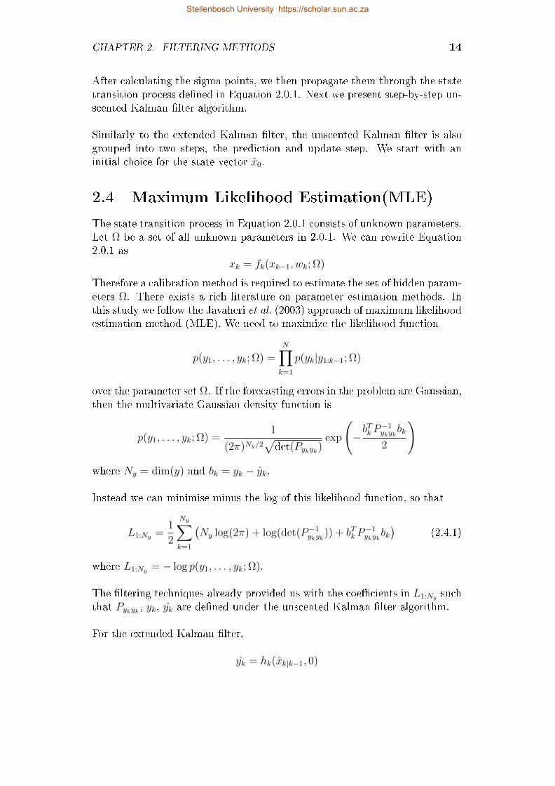
2.4 Maximum Likelihood Estimation(MLE)
The state transition process in Equation 2.0.1 consists of unknown parameters.Let Ω be a set of all unknown parameters in 2.0.1. We can rewrite Equation2.0.1 as
xk = fk(xk−1, wk; Ω)
Therefore a calibration method is required to estimate the set of hidden param-eters Ω. There exists a rich literature on parameter estimation methods. Inthis study we follow the Javaheri et al. (2003) approach of maximum likelihoodestimation method (MLE). We need to maximize the likelihood function
p(y1, . . . , yk; Ω) =N∏k=1
p(yk|y1:k−1; Ω)
over the parameter set Ω. If the forecasting errors in the problem are Gaussian,then the multivariate Gaussian density function is
p(y1, . . . , yk; Ω) =1
(2π)Ny/2√det(Pykyk)
exp
(−bTkP
−1ykyk
bk
2
)
where Ny = dim(y) and bk = yk − yk.
Instead we can minimise minus the log of this likelihood function, so that
L1:Ny =1
2
Ny∑k=1
(Ny log(2π) + log(det(P−1
ykyk)) + bTkP
−1ykyk
bk)
(2.4.1)
where L1:Ny = − log p(y1, . . . , yk; Ω).
The ltering techniques already provided us with the coecients in L1:Ny suchthat Pykyk , yk, yk are dened under the unscented Kalman lter algorithm.
For the extended Kalman lter,
yk = hk(xk|k−1, 0)
Stellenbosch University https://scholar.sun.ac.za

CHAPTER 2. FILTERING METHODS 15
Algorithm 3 Unscented Kalman lter algorithm
1: Step 1: Initialize
x0 = E[x0]
P0 = E[(x0 − x0)(x0 − x0)T ]
xa0 = E[xa0] =
x0
00
P a
0 = E[(xa0 − xa0)(xa0 − xa0)T ] =
P0 0 00 Pw 00 0 Pv
where Pw and Pv are the covariance of the state noise and measurementnoise respectively.
2: Step 2: Loop3: for k = 1 to Ny do
4: Sigma points:χak−1(0) = xak−1
for i = 1, . . . , L
χak−1(i) = xak−1 +(√
(L+ λ)P ak−1
)i
and for i = L+ 1, . . . , 2L
χak−1(i) = xak−1 −(√
(L+ λ)P ak−1
)i−L
where the subscripts i and i − L correspond to the ith and i − Lth
columns of the square-root matrix.5: Since χak−1 is known, we also know χxk−1, χ
wk−1, χ
vk−1:
χak−1 =
χxk−1
χwk−1
χvk−1
6: prediction step
7: Sigma points of xk:
χk|k−1(i) = f(χxk−1(i), χwk−1(i)) for i = 0, . . . , 2L.
8:
xk|k−1 =2L∑i=0
W(m)i χk|k−1(i)
9:
P−k =2L∑i=0
W(c)i
(χk|k−1(i)− xk|k−1
) (χk|k−1(i)− xk|k−1
)T10: Sigma points of yk
Yk|k−1(i) = h(χk|k−1(i), χvk−1(i))
Stellenbosch University https://scholar.sun.ac.za

CHAPTER 2. FILTERING METHODS 16
Algorithm 3 My algorithm (continued)
11:
yk =2L∑i=0
W(m)i (i)Yk|k−1(i)
12:
Pykyk =2L∑i=0
W(c)i
(Yk|k−1(i)− yk
) (Yk|k−1(i)− yk
)T13: Joint covariance of xk and yk is given by
Pxkyk =2L∑i=0
W(c)i
(χk|k−1(i)− xk|k−1
) (Yk|k−1(i)− yk
)T14: Update step
15: The Kalman gain is given by
Kk = PxkykP−1ykyk
16: The measurement residual
bk = yk − yk
17: The new state estimate
xk|k = xk|k−1 +Kkbk
18: Pk = P−k −KkPykykKTk
19: Then ultimately, set
xak = E[xak] =
xk|k00
P ak = E[(xak − xak)(xak − xak)T ] =
Pk 0 00 Pw 00 0 Pv
20: end for
Stellenbosch University https://scholar.sun.ac.za

CHAPTER 2. FILTERING METHODS 17
andPykyk = HkPk|k−1H
Tk + UkRkU
Tk
For further explanations on MLE for the extended and unscented Kalman l-ters, see Javaheri (2011) (pg 67-68).
The minimization of L1:N over the set of parameters Ω could be done via anumerical optimization routine such as the Nelder-Mead algorithm (Lagariaset al. (1998)), Secant-Levenberg-Marquardt method, the modied Sequen-tial Quadratic Programming (modSQP) method or the Simulated Annealingmethod, (see Kienitz and Wetterau (2012), Chapter 9). To obtain parame-ters, this study uses MATLAB's o-the-shelf" optimizer fminsearch and themodSQP method.
2.5 Particle Filter
Another popular ltering technique is the Sequential Monte Carlo methodknown as the particle lter. This method is widely used in uid mechan-ics. When a non-linear system is non-Gaussian then extended and unscentedKalman lters are not optimal methods to use. The particle lter methoduses Monte Carlo simulation to compute the posterior density function givenin Equation 2.0.3. Monte Carlo simulation is a well known approximationmethod which uses a set of well chosen random numbers. These random sam-ples are then used to approximate state distributions by performing many it-erations, where each iteration uses a dierent set of random values. Similarlyto the Monte Carlo, the particle lter approximate the state distributions witha nite set of weighted random samples drawn from a known, easy to sample,proposal distribution (q(x0:k|y1:t)). These random samples are called particlesand at time step k we might denote n particles for the state xk as
x(1)k , x
(2)k , . . . , x
(n)k .
The particles x(i)0:k for i = 1, . . . , n are independent and identically distributed.
Each particle is assigned an importance weight (rk) which determines its prob-ability of being sampled from the proposal distribution. The weighted set ofn particles at time step k will be denoted as x(i)
k , r(i)k for all i = 1, . . . , n.
The posterior density function from Equation 2.0.3 can be approximated asfollows
p(x0:k|y1:k) :=n∑i=1
r(i)k δ(x0:k − x(i)
0:k
)(2.5.1)
where δ(·) is a delta function. All we need to do to evaluate the transitionprobability in Equation 2.5.1, we need to generate a set of particles from a
Stellenbosch University https://scholar.sun.ac.za

CHAPTER 2. FILTERING METHODS 18
proposal distribution and iteratively compute the importance weights. This isgrouped into three steps:
1. Sampling
2. Computing the particle weights
3. Resampling.
The next subsections discuss the above steps in detail.
2.5.1 Sampling and computing the weights
The challenging part in implementing the particle lter, is the choice of theproposal distribution q(·) for generating particles. A proposal distributionshould contain the outputs of the posterior probability distribution and gener-ation of the samples should be done randomly. This has been a critical designissue and several proposal distributions are proposed in the literature. Luet al. (2015) discuss dierent proposal distributions for the particle lter andwhich are better suited to a particular target distribution. Dierent proposalfunctions based on the Kalman lter are proposed by Van Der Merwe et al.
(2000). In this study we use a proposal function by Doucet et al. (2000) givenas
q(xk|x0:k−1, y1:k) = p(xk|xk−1)
For each particle x(i)k (for i = 1, . . . , n) drawn from q(xk|x(i)
0:k−1, y1:k) has animportance weight dened by:
r(i)k = r
(i)k−1
p(yk|x(i)k )p(x
(i)k |x
(i)k−1)
q(x(i)k |x
(i)0:k−1, y1:k)
= r(i)k−1
p(yk|x(i)k )p(x
(i)k |x
(i)k−1)
p(x(i)k |x
(i)k−1)
= r(i)k−1p(yk|x
(i)k )
(2.5.2)
The importance weights are normalized, so that all the weights sum to 1,
r(i)k = r
(i)k
[n∑j=1
r(j)k
]−1
.
For further explanations on the particle lter, see Arulampalam et al. (2002),Van Der Merwe et al. (2000), Thrun (2002), and Doucet et al. (2000).
Stellenbosch University https://scholar.sun.ac.za

CHAPTER 2. FILTERING METHODS 19
2.5.2 Resampling
One of the major problems with particle ltering is particle degeneration. Thismeans that after several iterative procedures, a few importance weights becomevery large and all the other particles will have very small importance weightsto the point that they become negligible. This has a harmful eect on theaccuracy of the estimates, since a large number of particles (those with lowweights) are removed from the sample set. Degeneration of the particles hasan eect on computational time, since time will be wasted on low-weightedparticles that are no longer useful in the estimation. Resampling is a strategyproposed to reduce degeneration of particles.
In resampling, all the particles with low importance weights are eliminated anda new set of n equally weighted particles is drawn from the remained particles.A common way to measure the degeneracy is by an estimate of the eectivesample size given as follows
Neff =1∑n
i=1(rik)2.
The resampling step is taken when Neff < ne, where ne is usually set as n2.
At the end of the resampling procedure all the importance weights of the newparticles will be equal to 1/n. The importance weights are determined asfollows
r(i)k = r
(i)k =
1
n
For more details on resampling algorithms see Hol et al. (2006), Arulampalamet al. (2002) and Van Der Merwe et al. (2000).
2.5.3 The particle lter algorithm
From the previous subsection, we have explained how to generate particles froma proposal distribution. We also discussed how to compute their correspondingimportance weights. To avoid degeneracy of particles, resampling of particleswas also discussed. We now present algorithm of the particle lter as outlinedin Van Der Merwe et al. (2000).
Stellenbosch University https://scholar.sun.ac.za

CHAPTER 2. FILTERING METHODS 20
Algorithm 4 Particle lter algorithm
1: Initialize2: for k = 0 do
3: For i = 1, . . . , n, draw the state's particles x(i)0 from p(x0)
4: end for
5: for k = 1 to N do
6: (a) Sampling step
7: For i = 1, . . . , n, sample x(i)k from q(xk|x(i)
0:k−1, y1:k)8: For i = 1, . . . , n, compute the importance weights
r(i)k = r
(i)k−1
p(yk|x(i)k )p(x
(i)k |x
(i)k−1)
q(x(i)k |x
(i)0:k−1, y1:k)
9: For i = 1, . . . , n, normalize the importance weights
r(i)k = r
(i)k
[n∑j=1
r(j)k
]−1
10: (b) Resampling step11: if Neff < ne then
12: Eliminate particles x(i)k with low importance weights r
(i)k
13: Draw a new set of n equally weighted particles x(i)k approximately
14: distributed according to q(x(i)k |x
(i)k−1, y1:k)
15: For i = 1, . . . , n set r(i)k = r
(i)k = 1
n
16: else
17: Do nothing18: end if
19: (c) output20: Approximated posterior distribution
xk|k =n∑i=1
r(i)k x
(i)k
21: end for
Stellenbosch University https://scholar.sun.ac.za

CHAPTER 2. FILTERING METHODS 21
2.5.4 Maximum Likelihood Estimation for particle lter
For parameter estimation under the particle lter, we use the MLE method.Given a likelihood function at time step k
lk = p(yk|y1:k−1) =
ˆp(yk|xk)p(xk|y1:k−1)dxk
=
ˆp(yk|xk)
p(xk|y1:k−1)
q(xk|xk−1y1:k)q(xk|xk−1y1:k)dxk
=n∑i=1
p(yk|x(i)k )p(x
(i)k |x
(i)k−1)
q(x(i)k |x
(i)k−1)
the log-likelihood to be maximized is
ln(L1:n) =n∑k=1
ln(lk) (2.5.3)
and hence the parameters set Ω will be obtained using the same optimizationmethods as discussed in Section 2.4.
For further explanation of MLE under particle ltering, refer to Javaheri et al.(2003) and Javaheri (2011) (Page 102).
Stellenbosch University https://scholar.sun.ac.za

Chapter 3
Stochastic Volatility Models
The stock market crash of October 1987 caused investors to criticize the math-ematical models on their ability to price options. Options are perceived to becomplex derivatives due to the nancial crisis. The widely used Black-Scholes(1973) model assumes that the underlying volatility is constant over the lifeof the derivative. Empirical studies have shown that the Black-Scholes con-stant volatility does not hold in equity markets. Instead of getting horizontalgraphs of volatility vs maturity or volatility vs strike, various asset returnshave exhibited a nonlinear behaviour, sometimes like an upward (parabolic)smile. This has become known as the volatility smile. Half of a smile is re-ferred to as the volatility skew or volatility smirk. The quoted market pricesfor out-the-money put prices (and in-the-money call prices) are higher thanthe Black-Scholes prices (Christoersen et al. (2009)). Therefore, the Black-Scholes model does not adequately capture all the features observed in the op-tion market. To overcome this problem, recent studies assume return volatilityto be time-varying and predictable. Models with time-varying volatility whichare driven by their own stochastic processes are known as stochastic volatilitymodels.
Some of the widely used stochastic volatility models for pricing options are Hulland White (1987), Bates (1996), Heston (1993), Stein and Stein (1991) andScott (1987). The Heston (1993) model is one of the most popular stochasticvolatility models for pricing equity options. The choice of the Heston modelis motivated by its closed-form valuation formula that can be used to priceoptions. Risky asset returns that follow a normal distribution cannot fullyexplain some features such as the smile or skew of the implied volatilities ex-tracted from option prices. Under the Heston model, the underlying assetreturns exhibit a fatter tail distribution than that of a normal distribution.Hence, the Heston model is capable of generating smile or skew of the impliedvolatilities. Christoersen et al. (2009) proposed a two-factor model called theDouble Heston model. They argue that the Standard Heston (1993) modeldoes not always capture the dynamics of the term structure of implied volatil-
22
Stellenbosch University https://scholar.sun.ac.za

CHAPTER 3. STOCHASTIC VOLATILITY MODELS 23
ity very well, especially at short maturities. In the Double Heston model,an asset return is driven by two-factor stochastic volatility. This has the ad-vantage of improving the model's exibility in modelling the volatility termstructure.
In this chapter, we describe the Standard Heston model and its extension,the Double Heston model, in detail and present their characteristic functions,which are important in option valuations. We also present the state-spacerepresentations for these models, which we use in the ltering methods toestimate the volatilities.
3.1 The Heston Model
In this section, we rst present the dynamic system for the Heston model un-der a risk-neutral measure Q. Then lastly, we show how to price options underthe Heston model.
Under a risk-neutral measure Q, the Heston (1993) model assumes that anunderlying stock price, St has a stochastic variance, Vt, that follows a Cox,Ingersoll and Ross (1985) process. This process is represented by the followingdynamical system:
dSt = (r − q)Stdt+√VtStdWt (3.1.1)
dVt = κ(θ − Vt)dt+ σ√VtdZt, (3.1.2)
where r is a constant risk-free interest rate, q is a constant dividend, κ is amean reversion rate for the variance. The model mean reversion level for thevariance is denoted by θ and σ is a volatility of the variance. All the parame-ters κ, θ, σ are positive constant. The two independent Brownian motions Wk
and Zk are correlated with a constant correlation ρ ∈ [−1, 1].
For option valuation, we follow the Albrecher et al. (2006) approach, suchthat the characteristic function of log returns xk = ln(Sk/Sk−1) (for k ≤ t) ofthe Heston model is derived using the so called the little Heston trap. Thischaracteristic function is only slightly dierent from the original formulationof Heston (1993), but it provides a better computation of the numerical inte-gration. Heston (1993) provided the European call option closed-form solutiongiven by
C(S, V,K, τ) = Ske−qτP1 −Ke−rτP2 (3.1.3)
where K is the strike price, and probabilities
Pj =1
2+
1
π
ˆ ∞0
Re
[e−iφ lnKfj(φ;xk, Vk)
iφ
]dφ
Stellenbosch University https://scholar.sun.ac.za

CHAPTER 3. STOCHASTIC VOLATILITY MODELS 24
for j = 1, 2.
The characteristic functions fj(φ;xk, Vk) in the probabilities are given by
fj(φ, τ, xk, Vk) = eiφxk+Aj(φ,τ)+Bj(φ,τ)Vk
where
Bj(τ, φ) =bj − ρσφi+ dj
σ2
[1− edjτ
1− gjedjτ
],
Aj(τ, φ) = rφiτ +a
σ2
[(bj − ρσφi+ dj)τ − 2 ln
(1− gjedjτ
1− gj
)],
gj =bj − ρσφi+ djbj − ρσφi− dj
,
dj =√
(ρσφi− bj)2 − σ2(2ujφi− φ2),
and i =√−1, τ = T − k, u1 = 1
2, u2 = −1
2, a = κθ, b1 = κ− ρσ, b2 = κ and φ
is called the integration variable or node.
The European put options can be obtained via put-call parity. A number ofpapers have documented the derivations for the options premium under theHeston (1993) model as well the characteristic function see Heston (1993),Albrecher et al. (2006), (Rouah (2013), Chapter 1) and (Zhu (2009), Chapter3) for further discussions.
3.2 The Double Heston Model
The Double Heston model proposed by Christoersen et al. (2009), assumesthat the underlying stock price, St is driven by two independent factors ofvolatility, V 1
t and V 2t . Under a risk-neutral framework its dynamical system is
dened as follow:
dSt = (r − q)Stdt+√V 1t StdW
1t +
√V 2t StdW
2t ,
dV 1t = κ1(θ1 − V 1
t )dt+ σ1
√V 1t dZ
1t ,
dV 2t = κ2(θ2 − V 2
t )dt+ σ2
√V 2t dZ
2t ,
(3.2.1)
where r is a constant risk-free interest rate, q is a constant dividend-yield andother parameters also constant. The Brownian motions W 1
t , Z1t and W 2
t , Z2t
are correlated
d[W i, Zj]t = ρidt for all i = j
d[W i, Zj]t = 0 for all i 6= j
Stellenbosch University https://scholar.sun.ac.za

CHAPTER 3. STOCHASTIC VOLATILITY MODELS 25
for i, j = 1, 2. Note that the constant correlation parameters ρ1, ρ2 ∈ [−1, 1].
To determine the characteristic function for the Double Heston model, we rststate the multi-dimensional Feynman-Kac Theorem.
Theorem 3.1. Multi-dimensional Feynman-Kac Theorem
Let xk be an n−dimensional stochastic process with dynamics
dxk = µ(k, xk)dk + σ(k, xk)dWk (3.2.2)
where k ≤ t ≤ T ,
a column vector valued function µ(k, x1, . . . , xn) : R+ × Rn → Rn
a matrix valued function σ(k, x1, . . . , xn) : R+ × Rn → Rn×d
Wk is a d−dimensional Brownian motion with independent components
The innitesimal generator of the process in Equation 3.2.2 is dened by
A =n∑i=1
µi(k, x1, . . . , xn)
∂
∂xi+
1
2
n∑i,j=1
Cij∂2
∂xi∂xj(3.2.3)
where Cij = (σσT )ij.
Let f : Rn → Rn be a solution of the boundary value problem
∂f
∂t(t, x1, . . . , xn) +Af(t, x1, . . . , xn)− r(t, x1, . . . , xn)f(t, x1, . . . , xn) = 0
f(T, x1, . . . , xn) = Φ(x1, . . . , xn)
(3.2.4)
for a real valued functions r(k, x1, . . . , xn) : R+ × Rn → R and Φ(x1, . . . , xn) :Rn → R.
Then the solution f(t, x1, . . . , xn) is given by the expectation
f(t, x1, . . . , xn) = E[exp
(−ˆ T
t
r(k, xk)dk
)Φ(xT )
].
According to the Feynman-Kac Theorem 3.1, we know that f satises the PDF
∂f
∂t+Af − rf = 0 (3.2.5)
Stellenbosch University https://scholar.sun.ac.za
CHAPTER 3. STOCHASTIC VOLATILITY MODELS 26
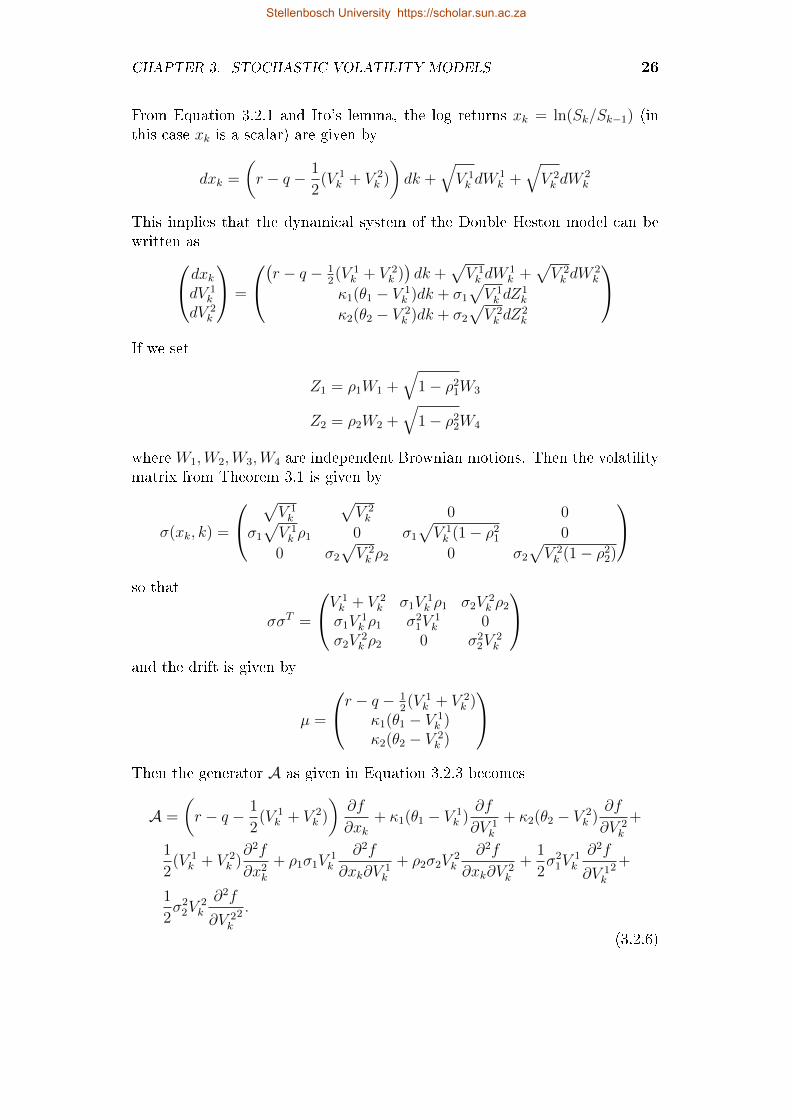
From Equation 3.2.1 and Ito's lemma, the log returns xk = ln(Sk/Sk−1) (inthis case xk is a scalar) are given by
dxk =
(r − q − 1
2(V 1
k + V 2k )
)dk +
√V 1k dW
1k +
√V 2k dW
2k
This implies that the dynamical system of the Double Heston model can bewritten asdxkdV 1
k
dV 2k
=
(r − q − 12(V 1
k + V 2k ))dk +
√V 1k dW
1k +
√V 2k dW
2k
κ1(θ1 − V 1k )dk + σ1
√V 1k dZ
1k
κ2(θ2 − V 2k )dk + σ2
√V 2k dZ
2k
If we set
Z1 = ρ1W1 +√
1− ρ21W3
Z2 = ρ2W2 +√
1− ρ22W4
where W1,W2,W3,W4 are independent Brownian motions. Then the volatilitymatrix from Theorem 3.1 is given by
σ(xk, k) =
√V 1k
√V 2k 0 0
σ1
√V 1k ρ1 0 σ1
√V 1k (1− ρ2
1 0
0 σ2
√V 2k ρ2 0 σ2
√V 2k (1− ρ2
2)
so that
σσT =
V 1k + V 2
k σ1V1k ρ1 σ2V
2k ρ2
σ1V1k ρ1 σ2
1V1k 0
σ2V2k ρ2 0 σ2
2V2k
and the drift is given by
µ =
r − q − 12(V 1
k + V 2k )
κ1(θ1 − V 1k )
κ2(θ2 − V 2k )
Then the generator A as given in Equation 3.2.3 becomes
A =
(r − q − 1
2(V 1
k + V 2k )
)∂f
∂xk+ κ1(θ1 − V 1
k )∂f
∂V 1k
+ κ2(θ2 − V 2k )
∂f
∂V 2k
+
1
2(V 1
k + V 2k )∂2f
∂x2k
+ ρ1σ1V1k
∂2f
∂xk∂V 1k
+ ρ2σ2V2k
∂2f
∂xk∂V 2k
+1
2σ2
1V1k
∂2f
∂V 1k
2 +
1
2σ2
2V2k
∂2f
∂V 2k
2 .
(3.2.6)
Stellenbosch University https://scholar.sun.ac.za

CHAPTER 3. STOCHASTIC VOLATILITY MODELS 27
Substituting A into Equation 3.2.5 gives us the double Heston model PDE.
Since the Double Heston model belongs to the class of ane models (Christof-fersen et al. (2009)), meaning that f has a closed-form solution with an expo-nential ane relationship to the state variables. This is given by the followingform
f(φ0, φ1, φ2;xk, V1k , V
2k ) = E
[exp(iφ0xT + iφ1V
1T + iφ2V
2T )]
= exp(A(τ) +B0(τ)xk +B1(τ)V 1k +B2(τ)V 2
k )
(3.2.7)
where τ = T − k.
The coecients A,B0, B1, B2 can be obtained as follows. We rst substituteEquation 3.2.7 for f in Equation 3.2.5 to obtain
f
[(∂A
∂k+∂B0xk∂k
+∂B1V
1k
∂k+∂B2V
2k
∂k
)+ µ1B0 + µ2B1 + µ3B2 +
1
2
((σσT )11B
20+
(σσT )22B21 + (σσT )33B
22 + (σσT )12B0B1 + (σσT )13B0B2
)]= 0
(3.2.8)
Note that µ and σσT are ane, such that
µ(xk) = K0 +K1x1 +K2V1k +K3V
2k
σ(xk)σ(xk)T = H0 +H1xk +H2V
1k +H3V
2k
where
K0 =
r − qκ1θ1
κ2θ2
, K1 =
000
, K2 =
−12
−κ1
0
, K3 =
−12
0−κ2
and
H0 = H1 =
0 0 00 0 00 0 0
, H2 =
1 σ1ρ1 0σ1ρ1 σ2
1 00 0 0
, H3 =
1 0 σ2ρ2
0 0 0σ2ρ2 0 σ2
2
.
Substituting the variables from µ and σσT in the Equation 3.2.8, we get
f
[∂A
∂k+∂B0xk∂k
+ (r − q)B0 + κ1θ1B1 + κ2θ2B2+
∂B1V1k
∂k+ V 1
k
(−1
2B0 − κ1B1 +
1
2B2
0 +1
2σ2
1B21 +
1
2σ1ρ1B0B1
)+
∂B2V2k
∂k+ V 2
k
(−1
2B0 − κ2B2 +
1
2B2
0 +1
2σ2
2B22 +
1
2σ2ρ2B0B2
)]= 0.
Stellenbosch University https://scholar.sun.ac.za

CHAPTER 3. STOCHASTIC VOLATILITY MODELS 28
We will drop f because it is always true that f > 0. In order for the driftterm to equal 0 for all values of xk, V
1k and V 2
k , their coecient terms and theconstants terms must sum to 0. That gives us the following system of ODEs
∂B0
∂k= 0
∂A
∂k+ (r − q)B0 + κ1θ1B1 + κ2θ2B2 = 0
∂B1
∂k− 1
2B0 − κ1B1 +
1
2B2
0 +1
2σ2
1B21 +
1
2σ1ρ1B0B1 = 0
∂B2
∂k− 1
2B0 − κ2B2 +
1
2B2
0 +1
2σ2
2B22 +
1
2σ2ρ2B0B2 = 0
(3.2.9)
These are Riccati equations for the Double Heston model. The solution to theseRiccati equations can be found in many textbooks on dierential equations.Rouah (2013) provided solutions to the Riccati equations for the StandardHeston model equations on Page 12 and 263. Rouah (2013) also argue thatB1 and B2 are identical to their counterparts in the Standard Heston model,therefore their solutions are
B0(τ) = 0
Bj(τ, φ) =κj − ρjσjφi+ dj
σ2j
[1− edjτ
1− gjedjτ
]A(τ, φ) = (r − q)φiτ +
2∑j=1
κjθjσ2j
[(κj − ρjσjφi+ dj)τ − 2 ln
(1− gjedjτ
1− gj
)](3.2.10)
where
gj =κj − ρjσjφi+ djκj − ρjσjφi− dj
dj =√
(κj − ρjσjφi)2 + σ2jφ(φ+ i)
for j = 1, 2.
With the known coecients A,B0, B1 and B2, we can now compute the char-acteristic function f . Christoersen et al. (2009) computed the price of a Eu-ropean call option under the Double Heston model via the Fourier inversionas
C(K) = Ske−qτP1 −Ke−rτP2
where K is the strike price, and
P1 =1
2+
1
π
ˆ ∞0
Re
[e−iφ lnKf(φ− i;xk, V 1
k , V2k )
iφSte−τ
]dφ
Stellenbosch University https://scholar.sun.ac.za
CHAPTER 3. STOCHASTIC VOLATILITY MODELS 29
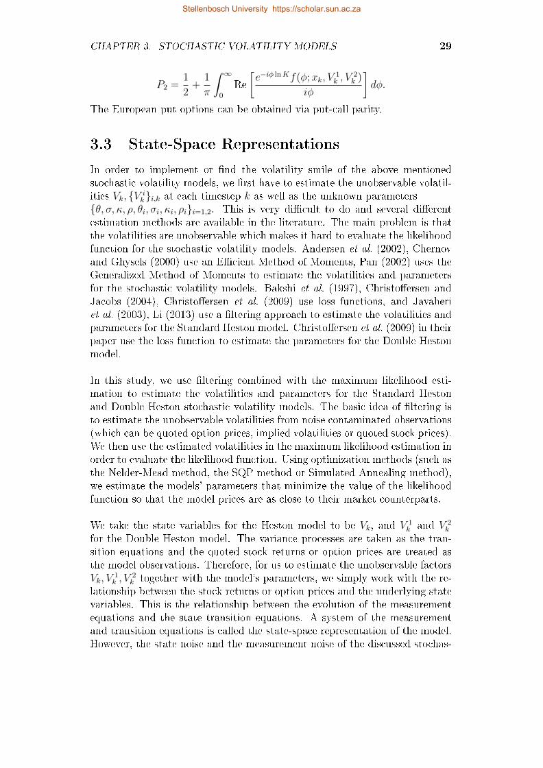
P2 =1
2+
1
π
ˆ ∞0
Re
[e−iφ lnKf(φ;xk, V
1k , V
2k )
iφ
]dφ.
The European put options can be obtained via put-call parity.
3.3 State-Space Representations
In order to implement or nd the volatility smile of the above mentionedstochastic volatility models, we rst have to estimate the unobservable volatil-ities Vk, V i
ki,k at each timestep k as well as the unknown parametersθ, σ, κ, ρ, θi, σi, κi, ρii=1,2. This is very dicult to do and several dierentestimation methods are available in the literature. The main problem is thatthe volatilities are unobservable which makes it hard to evaluate the likelihoodfunction for the stochastic volatility models. Andersen et al. (2002), Chernovand Ghysels (2000) use an Ecient Method of Moments, Pan (2002) uses theGeneralized Method of Moments to estimate the volatilities and parametersfor the stochastic volatility models. Bakshi et al. (1997), Christoersen andJacobs (2004), Christoersen et al. (2009) use loss functions, and Javaheriet al. (2003), Li (2013) use a ltering approach to estimate the volatilities andparameters for the Standard Heston model. Christoersen et al. (2009) in theirpaper use the loss function to estimate the parameters for the Double Hestonmodel.
In this study, we use ltering combined with the maximum likelihood esti-mation to estimate the volatilities and parameters for the Standard Hestonand Double Heston stochastic volatility models. The basic idea of ltering isto estimate the unobservable volatilities from noise contaminated observations(which can be quoted option prices, implied volatilities or quoted stock prices).We then use the estimated volatilities in the maximum likelihood estimation inorder to evaluate the likelihood function. Using optimization methods (such asthe Nelder-Mead method, the SQP method or Simulated Annealing method),we estimate the models' parameters that minimize the value of the likelihoodfunction so that the model prices are as close to their market counterparts.
We take the state variables for the Heston model to be Vk, and V 1k and V 2
k
for the Double Heston model. The variance processes are taken as the tran-sition equations and the quoted stock returns or option prices are treated asthe model observations. Therefore, for us to estimate the unobservable factorsVk, V
1k , V
2k together with the model's parameters, we simply work with the re-
lationship between the stock returns or option prices and the underlying statevariables. This is the relationship between the evolution of the measurementequations and the state transition equations. A system of the measurementand transition equations is called the state-space representation of the model.However, the state noise and the measurement noise of the discussed stochas-
Stellenbosch University https://scholar.sun.ac.za

CHAPTER 3. STOCHASTIC VOLATILITY MODELS 30
tic volatility models are correlated. Since for the lters the process noise andmeasurement noise must be uncorrelated, we will use Cholesky decompositionto decorrelate the sources of randomness.
Next we discuss the reformulation of our models in state-space representationwhich involves the specication of the measurement equations and state tran-sition equations. This is a crucial step for us to be able to do the model'sestimation using ltering. First we present the state-space form for the Hes-ton model, and lastly for the Double Heston model.
Under the Heston (1993) model, if we take the spot price Sk as the observationand the variance Vk as the state, then the measurement equation is representedby the stock price equation and the state transition equation by the varianceprocess. Recall that the Heston model is represented by a system of equations
Sk = lnSk−1 +
(r − q − 1
2Vk−1
)∆k +
√Vk−1
√∆kWk−1
Vk = Vk−1 + κ (θ − Vk−1) ∆k + σ√Vk−1
√∆kZk−1.
where Wk and Zk are correlated. To eliminate the correlation between theseequations, Javaheri (2011) (Page 87-88) shows that the best way to do this isby subtracting from the variance process f(xk−1, wk) a multiple of the quantityh(xk, vk)− yk, which is equal to zero. Writing
Vk =Vk−1 + (κθ − κVk−1)∆k + σ√Vk−1
√∆kZk−1
− ρσ[lnSk−1 +
(r − q − 1
2Vk−1
)∆k +
√Vk−1
√∆kBk−1 − lnSk
]which gives
Vk =Vk−1 +
[(κθ − ρσ(r − q))−
(κ− 1
2ρσ
)Vk−1
)∆k + ρσ ln
(SkSk−1
)+
σ√
1− ρ2√Vk−1
√∆kBk−1.
(3.3.1)
where
Bk =1√
1− ρ2(Zk − ρWk)
and the measurement equation is
yk = lnSk = lnSk−1 +
(r − q − 1
2Vk
)∆k +
√Vk√
∆kWk (3.3.2)
Equation 3.3.1 represents the state transition equation and clearly, Bk and Wk
are uncorrelated.
Stellenbosch University https://scholar.sun.ac.za

CHAPTER 3. STOCHASTIC VOLATILITY MODELS 31
Li (2013) suggested that if we take the spot prices Sk and option pricesC(Sk, K) as the observations and the variance Vk as the state, then the mea-surement equations are represented by
lnSk = lnSk−1 +(r − q − ρ
σκθ)
∆k +ρ
σVk +
[ρ
σ(κ∆k − 1)− 1
2∆k
]Vk−1+√
1− ρ2√
∆k√Vk−1Wk.
(3.3.3)
y0k = g(Sk, Vk,Θ) + ε0t (3.3.4)
where y0k is the observable option prices, with identical independent distributed
measurement errors ε0k → N (0, σ20), independent of Wk and Zk, and g(·) is the
theoretical option price computed from the Heston model.
The state transition equations are given by the variance processes(Vk
Vk−∆k
)=
(κθ∆k
0
)+
(1− κ∆k 0
1 0
)(Vk−∆k
Vk−2∆k
)+
(σ√
∆kVk−∆k
0
)Zk
See Li (2013) for the derivation of Equations 3.3.3.
Under the Double Heston model, recall that the system equations are
lnSk = lnSk−1 +
((r − q)− 1
2(V 1
k + V 2k )
)dk +
√V 1k dW
1k +
√V 2k dW
2k ,
V 1k = V 1
k−1 + κ1(θ1 − V 1k−1)4 k + σ1
√V 1k−1
√4kZ1
k ,
V 2k = V 2
k−1 + κ2(θ2 − V 2k−1)4 k + σ2
√V 2k−1
√4kZ2
k .
(3.3.5)
Suppose we take the spot price Sk as the observation and the variance pro-cesses V 1
k , V2k as the states, then the measurement equation is represented by
the stock price lnSk in Equation 3.3.5 and the transition equations by thevariance processes V 1
k , V2k in Equation 3.3.5. The problem we face when using
these equations, the process noise and the measurement noise are correlated,d[W 1, Z1]k = ρ1dk and d[W 2, Z2]k = ρ2dk. However, for the ltering the pro-cess and the measurement noises must be uncorrelated.
Next we derive the measurement equations and the state transition equationsfor the Double Heston model to t into the ltering such that the process noiseand the measurement noise are uncorrelated.
By Ito's Lemma, we let xk = ln( Sk
Sk−1). This implies that
dxk =
(r − q − 1
2(V 1
k + V 2k )
)dk +
√V 1k dW
1k +
√V 2k dW
2k (3.3.6)
Stellenbosch University https://scholar.sun.ac.za

CHAPTER 3. STOCHASTIC VOLATILITY MODELS 32
By using the Cholesky decomposition, we set
dW 1k = ρ1dZ
1k +
√1− ρ2
1dZ1k
dW 2k = ρ2dZ
2k +
√1− ρ2
2dZ2k
where d[Z1, Z1] = d[Z2, Z2] = 0
Substituting dW 1k , dW
2k in Equation 3.3.6, we get
dxk =
(r − q − 1
2(V 1
k + V 2k )
)dt+
√V 1k
(ρ1dZ
1k +
√1− ρ2
1dZ1k
)+√
V 2k
(ρ2dZ
2k +
√1− ρ2
2dZ2k
)=
(r − q − 1
2(V 1
k + V 2k )
)dk + ρ1
√V 1k dZ
1k +
√1− ρ2
1
√V 1k dZ
1k+
ρ2
√V 2k dZ
2k +
√1− ρ2
2
√V 2k dZ
2k .
(3.3.7)
From Equation 3.2.1, we know that√V 1k dZ
1k =
1
σ1
(dV 1
k − κ1(θ1 − V 1k )dk
)(3.3.8)√
V 2k dZ
2k =
1
σ2
(dV 2
k − κ2(θ2 − V 2k )dk
)(3.3.9)
By substituting Equation 3.3.8 and 3.3.9 into 3.3.7, we get
dxk =
(r − q − 1
2(V 1
k + V 2k )
)dk +
ρ1
σ1
(dV 1
k − κ1(θ1 − V 1k )dk
)+√
1− ρ21
√V 1k dZ
1k +
ρ2
σ2
(dV 2
k − κ2(θ2 − V 2k )dk
)+√
1− ρ22
√V 2k dZ
2k .
Rearranging this and substituting xk = ln( Sk
Sk−1), we get
lnSk = lnSk−1 +
(r − q − ρ1
σ1
κ1θ1 −ρ2
σ2
κ2θ2
)4 k +
ρ1
σ1
V 1k +
ρ2
σ2
V 2k +(
ρ1
σ1
(κ14 k − 1)− 1
24 k
)V 1k−1 +
(ρ2
σ2
(κ24 k − 1)− 1
24 k
)V 2k−1+√
1− ρ21
√V 1k−1
√4kZ1
k +√
1− ρ22
√V 2k−1
√4kZ2
k .
(3.3.10)
which is the measurement equation.
Stellenbosch University https://scholar.sun.ac.za

CHAPTER 3. STOCHASTIC VOLATILITY MODELS 33
The state transition equations are:
(V 1k
V 2k
)=
V 1k−1 + κ1(θ1 − V 1
k−1)4 k + σ1
√V 1k−1
√4kZ1
k
V 2k−1 + κ2(θ2 − V 2
k−1)4 k + σ2
√V 2k−1
√4kZ2
k
(3.3.11)
Clearly, the measurement noise Z1k and Z
2k from in Equation 3.3.10 are uncor-
related to the states noise Z1k , Z
2k in Equation 3.3.11.
Having reformulated the measurement equations and the state transition equa-tions for a model, its very important to know if the measurement equationscontains enough information to allow the estimation of the states. We needto check if it is possible to estimate the states from the given measurementequation(s). If the measurement equation y = 0, for instance, then it is notpossible to nd the state variables from this measurement equation, because itcontains not enough information about the states. A system that allows statesestimation from the measurement equation(s) is referred to as observable. Wetherefore need to check if the measurement equation given in Equation 3.3.10and the states in Equation 3.3.11 form an observable system. Below we pro-vide a mathematical denition of the observability of a system.
A nonlinear system with a state vector xk of dimension n is observable if
O =
H
HAHA2
...HAn−1
has a full rank of n. H and A are the Jacobian matrices of the measurementand the states as dened in Chapter 2, under the extended Kalman lter. Formore details on Observability, see Reif et al. (1999), Sira-Ramirez (1988) andHermann and Krener (1977).
Now we have a look at the observability of the measurement and transitionequations in Equations 3.3.10 and 3.3.11 respectively.
Since
H =( ρ1σ1
(κ14 k − 1)− 124 k ρ2
σ2(κ24 k − 1)− 1
24 k
),
then the observation matrix is
O =
( ρ1σ1
(κ14 k − 1)− 124 k ρ2
σ2(κ24 k − 1)− 1
24 k(
ρ1σ1
(κ14 k − 1)− 124 k
)(1− κ14 k) 0
).
Stellenbosch University https://scholar.sun.ac.za

CHAPTER 3. STOCHASTIC VOLATILITY MODELS 34
For 4k = 0, then
O =
( ρ1σ1
ρ2σ2
ρ1σ1
0
),
det(O) = − ρ1ρ2σ1σ2
< 0. So for small 4k, det(O) 6= 0 and hence O is non-singularfor small 4k and since it is a 2 × 2, then its rank must be 2. Therefore oursystem is observable.
Now suppose we take the spot price Sk and the option prices C(Sk, K) as theobservations and the variance processes V 1
k , V2k as the states, then the measure-
ment equations can be derived in the same way as was done for the StandardHeston model in Li (2013). We simply replace the Heston model theoretical op-tion price g(·) with the one for the Double Heston model. These measurementand the state transition equations are then used in the extended, unscentedKalman lter and the particle lter to estimate the model's volatilities and theparameters.
Stellenbosch University https://scholar.sun.ac.za

Chapter 4
Empirical Analysis
In Chapter 2, we discussed ltering methods. We also discussed two stochasticvolatility models and their characteristic functions in Chapter 3. The idea is toimplement these stochastic volatility models which have a volatility driven by atime-varying variance process. Unlike the Standard Heston model, the DoubleHeston model is driven by two variance processes. These variance processesconsist of unknown parameters. Therefore, implementing stochastic volatilitymodels is dicult since the volatilities are unobservable and parameters arehidden.
In this chapter we use the three non-linear ltering methods on options data.With these methods we extract the model's implied volatilities and comparetheir performance. We also combine the lters with the maximum likelihoodestimation method to estimate the hidden parameters.
In Section 4.1 we present our data set, Section 4.2 discusses about the Jacobianmatrices in the extended Kalman lter. Section 4.3 details the estimatedparameters under the Standard Heston model as well as the comparisons ofthe term structures of the extracted implied volatilities and the market impliedvolatilities. Section 4.4 presents the estimated parameters under the DoubleHeston model as well as the term structures of the extracted implied volatilitiesand the market implied volatilities. All the experiments are done in Matlab.
4.1 Data
In this study, the data used is put option prices on the Dow Jones IndustrialAverage ETF (DJIA), recorded on May 10, 2012. There are four maturities37, 72, 135, and 226 days. The closing price is $129.14 and the strikes pricesranges from K = 124 to K = 136 in increments of $1. The options dataset isquoted as implied volatility, as presented in Table 4.1.
35
Stellenbosch University https://scholar.sun.ac.za

CHAPTER 4. EMPIRICAL ANALYSIS 36
Table 4.1: DJIA Implied volatilities on 10 May 2012
Strike Maturity(Days)K 37 72 135 226
124 0.1962 0.1947 0.2019 0.2115125 0.1910 0.1905 0.1980 0.2082126 0.1860 0.1861 0.1943 0.2057127 0.1810 0.1812 0.1907 0.2021128 0.1761 0.1774 0.1871 0.200129 0.1718 0.1743 0.1842 0.1974130 0.1671 0.1706 0.1813 0.1950131 0.1644 0.1671 0.1783 0.1927132 0.1645 0.1641 0.1760 0.1899133 0.1661 0.1625 0.1743 0.1884134 0.1701 0.1602 0.1726 0.1862135 0.1755 0.1610 0.1716 0.1846136 0.1796 0.1657 0.1724 0.1842
We obtain this dataset from the Fabrice Douglas Rouah website Rouah (2013(accessed September 3, 2015) in his MATLAB codes titled the Heston modeland its extensions in Matlab and C#, chapter 9, script name: Mikhailov No-gel estimation DJIA. We use this data in our study for empirical analysis only,dierent quoted data can be used for implementations.
Since the options dataset is quoted as implied volatilities, to obtain the marketput prices, we use the Black-Scholes formula,
C = Se−qTN(d1)−Ke−rTN(d2),
P = Ke−rTN(−d2)− Se−qTN(−d1),
where C and P are the call and put prices, respectively. The stock closing priceis denoted by S, q is the expected dividend rate, r is a risk-free interest rate,T is the maturity, and K is the strike price. We also denoted the cumulativeprobability distribution function for standard normal distribution asN(·), withthe d1 and d2 dened as follows
d1 =ln(S/K) + (r − q + V 2/2)T
V√T
andd2 = d1 − V
√T ,
where V is the quoted implied volatility.
Stellenbosch University https://scholar.sun.ac.za

CHAPTER 4. EMPIRICAL ANALYSIS 37
4.2 Fitting lters
In Chapter 3 we have derived the state-space representations of the StandardHeston (1993) and Double Heston models. The state transition and mea-surement equations for these models are uncorrelated. All the lters wereinitialized at the unconditional means and covariance of the states. For theStandard Heston (1993) model, the mean was initialized by x0 = V0 and theinitial covariance P−0 = diag(σ2∆kV0, 0), where V0 is the initial level of thevariance. Recall that xk are the unobservable volatilities.
For the Double Heston model, the initial mean is
x0 =[V 1
0 , V2
0
]Tand the covariance P−0 = diag(σ2
1∆kV 10 , σ
22∆kV 2
0 ), where V 10 and V 2
0 are theinitial levels of the variance processes.
The Standard Heston model parameters to be estimated are κ, θ, σ, V0, ρ. Theparameters for the Double Heston model are κ1, θ1, σ1, V
10 , ρ1, κ2, θ2, σ2, V
20 , ρ2.
In the estimation, we keep the parameters xed at all the maturities. We rstinitialize the parameters and use the lters to estimate the volatilities and thenuse the MLE for valuation of the likelihood function. Optimization routines(see Section 2.4) are then used to estimate the best parameters that maximizethe likelihood function.
The volatilities xk are estimated using the ltering techniques discussed inChapter 2. The state transition and measurement equations are as discussedin Section 3.3.1. In this study we use option prices only as the observations,with the put option price given by
y0k = g(S, Vk,Θ) + ε0t
= C(K) +Ke−rτ − Ske−qτ + ε0t ,(4.2.1)
where y0k represents the put option price under the Standard Heston model,
C(K) is the call price as dened in Equation 3.1.3, and Θ is the set of modelparameters.
The Jacobian matrices in the extended Kalman lter under the Heston modelare given by
Ak = 1− κ∆k,
Wk = σ√Vk−1
√∆k
To compute the gradient matrix Hk of y0k with respect to the implied volatility
is not straight forward. We follow the approach of Zhu (2009) (Page 82-83).
Stellenbosch University https://scholar.sun.ac.za

CHAPTER 4. EMPIRICAL ANALYSIS 38
Rouah (2013) (Page 329) also used the same approach. Since the stock returnsvolatility is driven by a variance process which consists of parameters, Zhu(2009) recommends the derivatives of the call and put price with respect tothe implied volatility to be based on two parameters, ν1 = V0 the initial levelof the variance, and ν2 = θ the long term level of the variance. Therefore, theJacobian matrices of the put option with respect to the volatility
H1 =∂y0
k
∂ν1
=∂y0
k
∂V0
2√V0
H2 =∂y0
k
∂ν2
=∂y0
k
∂θ2√θ
(4.2.2)
Substitute the y0k from Equation 4.2.1 into Equation 4.2.2, yields
H1 = Se−qτ∂P1
∂V0
2√V0 −Ke−rτ
∂P2
∂V0
2√V0
where
∂Pj∂V0
=1
π
ˆ ∞0
Re
[e−iφ lnKfj(φ;Sk, Vk)Bj(τ, φ)
iφ
]dφ,
for j = 1, 2 and Bj(τ, φ) as dened in Section 3.1. The derivative of the secondJacobian matrix,
H2 = Se−qτ∂P1
∂θ2√θ −Ke−rτ ∂P2
∂θ2√θ
where
∂Pj∂θ
=1
π
ˆ ∞0
Re
[e−iφ lnKfj(φ;Sk, Vk)Aj(τ, φ)/∂θ
iφ
]dφ
and
∂Aj(τ, φ)
∂θ=
κ
σ2
[(bj − ρσφi+ dj)τ − 2 ln
(1− gjedjτ
1− gj
)].
Under the Double Heston model, the put option price is given by
y0k = g(S, V 1
k , V2k ,Θ) + ε0t
= C(K) +Ke−rτ − Ske−qτ + ε0t .(4.2.3)
The Jacobian matrices in the extended Kalman lter under the Double Hestonmodel are given by
A1 = 1− κ1∆k, A2 = 1− κ2∆k
W1 = σ1
√V 1k
√∆k, W2 = σ2
√V 2k
√∆k
Stellenbosch University https://scholar.sun.ac.za

CHAPTER 4. EMPIRICAL ANALYSIS 39
Since the Double Heston model has two initial variance parameters V 10 and
V 20 , then the derivatives of the put price with respect to the implied volatility
is based on ν1 =√V 1
0 and ν2 =√V 2
0 . These Jacobian matrices are given as
Hj = Se−qτ∂P1
∂V j0
2
√V j
0 −Ke−rτ∂P2
∂V j0
2
√V j
0
where
∂P1
∂V j0
=1
π
ˆ ∞0
Re
[e−iφ lnK
iφSke(r−q)τ f(φ− i;Sk, V 1k , V
2k )Bj(τ, φ− i)
]dφ,
∂P2
∂V j0
=1
π
ˆ ∞0
Re
[e−iφ lnK
iφf(φ;Sk, V
1k , V
2k )Bj(τ, φ)
]dφ,
for j = 1, 2 and Bj(τ, φ) as dened in Equation 3.2.10.
For the computation of Hk's we use the central-dierence method. The calcu-lation of the put price requires the evaluation of the integral of the characteris-tic functions. We use a numerical approximation method, the Gauss-LaguerreQuadrature. This method is well-suited in our integral, because it does notrequire lower and upper limits of the integration. In our case the integrationdomain is (0,∞) which can be challenging in choosing the lower and upperlimits.
4.3 Parameters in the Heston model
The estimated parameters κ, θ, σ, V0, ρ of the Standard Heston model from theextended Kalman lter (EKF), the unscented Kalman lter (UKF) and theparticle lter (PF) are found in Table 4.2. We estimated the parameters usingoptions on strike prices K = 124 : 134 only, leaving out options on strike prices135 and 136.
Table 4.2: Estimated parameters for the Heston model
κ θ σ V0 ρ
EKF 0.2898 0.1258 1.4002 0.0356 -0.426UKF 0.7782 0.2012 1.6699 0.0369 -0.4107PF 1.3421 0.1304 1.3568 0.0356 -0.4192
We obtained nearly the same parameters from both optimizations methods,therefore we only present the parameters from the fminsearch optimizer. Theparameters for the extended Kalman lter and the particle lters are nearly
Stellenbosch University https://scholar.sun.ac.za

CHAPTER 4. EMPIRICAL ANALYSIS 40
the same. It is not necessary for dierent lters to have same parameters. Themean reversion speed κ and the volatility of the variance σ control curvatureof the volatility smile. A higher value of κ atters the volatility smile anda higher value of σ increases the curvature of the smile. The parameters θand V0 determine the level of the smile, with a higher value of V0 leading to ahigher volatility σ. The correlation parameter ρ controls the direction of theimplied volatility smile. A negative ρ yields a negative slope of the smile anda positive ρ yields a positive slope.
Fig. 4.1 plots the term structure for the market implied volatilities and theextracted implied volatilities under the Standard Heston model.
125 130 135
0.16
0.18
0.2
0.22Maturity 37 days
HestonMarket
125 130 135
0.16
0.18
0.2
0.22Maturity 72 days
HestonMarket
125 130 135
0.16
0.18
0.2
0.22Maturity 135 days
HestonMarket
125 130 135
0.16
0.18
0.2
0.22Maturity 226 days
HestonMarket
Figure 4.1: Heston implied volatilities from EKF
The implied volatilities in Fig. 4.1 from the extended Kalman lter do nott the actual implied volatilities well especially at short maturities. In thematurities of 37 and 72 days, the Heston model completely failed to capturethe market implied volatilities. At long maturities (135 and 226 days) we geta better t compared to 37 and 72 days. The extended Kalman lter has alower κ which saddles the implied volatilities smile.
The term structure for the implied volatilities of the Standard Heston modelextracted by the unscented Kalman lter are found in Fig. 4.2. As shown in
Stellenbosch University https://scholar.sun.ac.za

CHAPTER 4. EMPIRICAL ANALYSIS 41
Fig. 4.2, the unscented Kalman lter provides a better t for the volatilitysmile at long maturities, 135 and 226 days. The short maturities still failed tocapture the smile. In the unscented Kalman lter the computation was donesetting α = 10−3, κ = 0 and β = 2.
125 130 135
0.15
0.2
0.25
Maturity 37 days
UKFMarket
125 130 135
0.15
0.2
0.25
Maturity 72 days
UKFMarket
125 130 135
0.15
0.2
0.25
Maturity 135 days
UKFMarket
125 130 135
0.15
0.2
0.25
Maturity 226 days
UKFMarket
Figure 4.2: Heston implied volatilities from UKF
The term structure for the implied volatilities of Heston model extracted us-ing particle lter are found in Fig. 4.3. Based on the results in Fig. 4.2 and4.3, it can be dicult to notice the dierence in the implied volatilities givenby the unscented Kalman and particle lters. However possible dierences, ifany, should become clear once a highly non-linear or a non-Gaussian modelis introduced. In the particle lter 500 particles were used and this was morecomputational demanding and took longer than the unscented Kalman lter.
When we estimated the parameters in Table 4.2 we left out option prices forthe strike prices K = 135 and 136. In Table 4.3 we present the Heston modelput option prices for the strike prices K = 135 and 136. These put prices arecomputed using estimated parameters in Table 4.2. Each strike price has fourmaturity days, namely 37, 72, 135, and 226. The closing price is S = 129.14.
Stellenbosch University https://scholar.sun.ac.za

CHAPTER 4. EMPIRICAL ANALYSIS 42
125 130 135
0.15
0.2
0.25
Maturity 37 days
PFMarket
125 130 135
0.15
0.2
0.25
Maturity 72 days
PFMarket
125 130 135
0.15
0.2
0.25
Maturity 135 days
PFMarket
125 130 135
0.15
0.2
0.25
Maturity 226 days
PFMarket
Figure 4.3: Heston implied volatilities from PF
Table 4.3: Put option prices from the Heston model
Filter Strike Maturity (Days)(K) 37 72 135 226
Actual Data 135 6.814255 7.504627 9.091425 11.199449136 7.674530 8.354330 9.816700 11.849407
EKF 135 7.084522 7.849682 9.021301 10.594243136 7.941194 8.681519 9.814157 11.342153
UKF 135 6.668625 7.434077 8.771653 11.384425136 7.521106 8.228892 9.488230 11.335073
PF 135 6.636029 7.471980 8.953781 11.027706136 7.478933 8.239642 9.635039 11.644477
4.4 Parameters in the Double Heston model
The estimated parameters κ1, θ1, σ1, V1
0 , ρ1, κ2, θ2, σ2, V2
0 , ρ2 for the extendedKalman lter (EKF), the unscented Kalman lter (UKF) and the particle l-ter (PF) under the two-factor model are found in Table 4.4. Similarly to theStandard Heston model, the parameters in the Double Heston model are alsoestimated using options on strike prices K = 124 : 134 only, leaving out op-tions on strike prices 135 and 136.
Stellenbosch University https://scholar.sun.ac.za

CHAPTER 4. EMPIRICAL ANALYSIS 43
Table 4.4: Estimated parameters for the Double Heston model
Parameter EKF UKF PF
κ1 3.0769 3.2381 3.0853θ1 0.0312 0.0307 0.0310σ1 2.0207 1.9898 2.0023V 1
0 0.0261 0.02721 0.0260ρ1 -0.0654 0.0604 0.0649κ2 1.8668 1.8131 1.8628θ2 0.0600 0.0583 0.0610σ2 0.6982 0.7105 0.7021V 2
0 0.0093 0.0095 0.0093ρ2 -0.9925 -1.0 -0.9836
As shown in Table 4.4 the parameters for all the lters are nearly the same.From Table 4.2 the correlation parameter ρ under the Heston model is alwaysnegative. Under the Double Heston model the correlation parameters ρ1 andρ2 can be negative or positive as shown on Table 4.4. The empirical studiesalso show that the market data yields negative as well as positive correlations.We therefore expect the Double Heston model to perform better than the Stan-dard Heston model. The long-term variance level θ2 of the second volatilityfactor controls the level of the implied volatility smile at short maturities andθ1 controls the level of the smile for longer maturities.
Fig. 4.4 plots the implied volatilities smile of the Double Heston model ex-tracted using the extended Kalman lter and the market implied volatilitiessmile. The results show a poor t of the extended Kalman lter on the DoubleHeston model. This also shows the extended Kalman lter weakness on highlynon-linear models. The linearization of the Double Heston model put optionequation might have also contributed errors. The volatility smile under theDouble Heston model at shorter maturities is better than under the StandardHeston model.
In Fig. 4.5 we present the implied volatilities under the Double Heston modelestimated by the unscented Kalman lter. The estimates are better than forthe extended Kalman lter. During estimation we set α = 0.99, κ = 0 andβ = 2, which implies that under the Double Heston model the sigma pointsare widely spread for better estimates. Implied volatilities estimated via theunscented Kalman lter do not t the market implied volatilities very wellespecially in the longer maturity of 226 days as shown in Fig. 4.5.
Fig. 4.6 displays the implied volatilities under the Double Heston model es-timated by the particle lter. We obtained nearly a perfect t at all maturi-
Stellenbosch University https://scholar.sun.ac.za

CHAPTER 4. EMPIRICAL ANALYSIS 44
125 130 135
0.16
0.18
0.2
0.22Maturity 37 days
DoubleMarket
125 130 135
0.16
0.18
0.2
0.22Maturity 72 days
DoubleMarket
125 130 135
0.16
0.18
0.2
0.22Maturity 135 days
DoubleMarket
125 130 135
0.16
0.18
0.2
0.22Maturity 226 days
DoubleMarket
Figure 4.4: Double Heston model Implied volatilities under EKF
125 130 1350.1
0.15
0.2
0.25
Maturity 37 days
double HestonMarket
125 130 1350.1
0.15
0.2
0.25
Maturity 72 days
double HestonMarket
125 130 1350.1
0.15
0.2
0.25
0.3Maturity 135 days
double HestonMarket
125 130 1350.1
0.15
0.2
0.25
0.3Maturity 226 days
double HestonMarket
Figure 4.5: The Double Heston model implied volatilities under UKF
Stellenbosch University https://scholar.sun.ac.za

CHAPTER 4. EMPIRICAL ANALYSIS 45
125 130 135
0.15
0.2
0.25
Maturity 37 days
Double PFMarket
125 130 135
0.15
0.2
0.25
Maturity 72 days
Double PFMarket
125 130 135
0.15
0.2
0.25
Maturity 135 days
Double PFMarket
125 130 135
0.15
0.2
0.25
Maturity 226 days
Double PFMarket
Figure 4.6: The Double Heston model implied volatilities under PF
ties. Furthermore, the Standard Heston model could not capture the smile atshorter maturities. Therefore, the Double Heston model oers more exibilityin modelling the volatility than the Standard Heston model. In the iterationwe used 500 particles.
Table 4.5 displays the Double Heston model put option prices for strike pricesK = 135 and 136. We computed the prices using the estimated parametersin Table 4.4. Compared to the Heston model prices in Table 4.3, the DoubleHeston model put prices are closer to the actual prices. The unscented Kalmanlter and the particle lter also performed better than the extended Kalmanlter in both models.
Stellenbosch University https://scholar.sun.ac.za

CHAPTER 4. EMPIRICAL ANALYSIS 46
Table 4.5: Put option prices from the Double Heston model
Filter Strike Maturity (Days)(K) 37 72 135 226
Actual Data 135 6.814255 7.504627 9.091425 11.199449136 7.674530 8.354330 9.816700 11.849407
EKF 135 6.834805 7.580502 8.973786 11.033095136 7.713028 8.403014 9.672677 11.642593
UKF 135 6.812425 7.578929 9.059128 11.200290136 7.691932 8.389437 9.743906 11.808492
PF 135 6.810771 7.592233 9.091525 11.249225136 7.688207 8.399582 9.778391 11.860654
Stellenbosch University https://scholar.sun.ac.za

Chapter 5
Conclusion
Many stochastic volatility models have been developed in the last decade,but the standard Heston model has emerged as the most popular stochasticvolatility model in option pricing theory. The Double Heston model whichwas proposed recently has also attracted the attention of traders. In thisdissertation we have studied and implemented these two stochastic volatilitymodels. In general, the implementation of the stochastic volatility models isquite challenging, as one is confronted with the diculty of jointly estimatingthe models' hidden parameters, as well as the unobservable volatilities. Theunobservable volatilities were estimated through the ltering approach usingmarket option prices. Filtering methods are considered to be ecient in distin-guishing unobservable state variables from noisy observations, regardless of theobservations size. These methods converge faster to the true values comparedto other methods, like Monte Carlo, that require large numbers of simulationsfor better estimation.
The study began with a brief discussion of the ltering methods. For betterunderstanding of the lters we began with the Kalman ltering. This lteringmethod was not used in the implementation, because our models are non-linearand it is only optimal for linear models. The other ltering methods discussedare the extended Kalman lter, the unscented Kalman lter and the particlelter. Our numerical results for comparison show that the particle lter per-forms better compared to the other lters. Under the Standard Heston model,the implied volatilities from the particle lter and the unscented Kalman lterare almost the same. The dierence between the unscented Kalman lter andthe particle lter became clear under the Double Heston model. The extendedKalman lter performed poorly for both models. The results also show thatthe Double Heston model ts the market implied volatility smile very well atall maturities. The Standard Heston model fails to explain the random move-ments in the implied volatilities smile at shorter maturities. Therefore, theDouble Heston model has introduced more exibility in modelling the volatil-ity.
47
Stellenbosch University https://scholar.sun.ac.za

CHAPTER 5. CONCLUSION 48
The particle lter has been criticised for its degeneracy problem. To avoiddegeneracy, one can consider a good choice of the proposal distribution or in-cluding the resampling step in the algorithm. In this study we used both theproposal distribution and the resampling step, and this makes particle lteringmore ecient. The approximation of the Jacobian matrices in the extendedKalman lter are done using the central-dierence method. The maximumlikelihood estimation method was used to estimate the model's parameters.
Future work includes the use of lters on estimating implied volatilities aswell the parameters under the stochastic volatility models using options onFTSE/JSE Top 40 index (ALSI) quoted on 05 Feb 2013. We already obtainedthe data from Johannesburg Stock Exchanges (JSE).
Stellenbosch University https://scholar.sun.ac.za

Appendix A
Kalman lter
This appendix derives the prediction and update equations in the Kalmanlter algorithm. The derivations were created by my project supervisor. Werst start with some properties in probability.
A.1 Probability properties
If Z = X + Y , all three being vectors of the same length whose elements arerandom variables with zero means, and X, Y are independent then
cov(Z) = cov(X) + cov(Y )
where cov(X) = E(XXT
)and similarly for Y, Z. If X is deterministic then
cov(Z) = cov(Y ). If X does not have zero mean then
cov(X) = E((X − E(X))(X − E(X))T )
If X, Y have mean X, Y then
E((X − X)(Y − Y )T ) = E(XY T )− XY T
If X has zero mean and A a deterministic matrix such that AX is dened then
cov(AX) = E((AX)(AX)T ) = E(AXXTAT ) = AE(XXT )AT = Acov(X)AT .
If X ∼ N(µ,Σ is normal then AX is also normal and AX ∼ N(Aµ,AΣAT ).
If X, Y have lengths m,n respectively then cov(X, Y ) is an m× n matrix.
Let X,Z, (X,Z)T be vectors of random variables, with Z multivariate normalsatisfying (
XZ
)= N
( (µXµZ
),
(A BC D
) )49
Stellenbosch University https://scholar.sun.ac.za

APPENDIX A. KALMAN FILTER 50
where A,D are square and have the same number of rows as X, Y respectively,and D is invertible.
Then A = cov(X) = P xx, D = cov(Z) = P zz, B = cov(X,Z) = P xz, C =cov(Z,X) = P zx.
If X conditioned on Z = z is written as (X|Z = z), then it satises
(X|Z = z) ∼ N(µX +BD−1(z − µZ), A−BD−1C)
A.2 Kalman ltering
Consider n−vectors xk, yk, wk, vk, deterministic n×nmatricesM andHk and n × n positive denite matrices Q,R (k = 0, 1, 2, . . . ), and deter-ministic n−vectors Ck, Dk.
xk is the internal state of a system and satises
xk = Axk−1 + Ck + wk
x0 may be unknown.
yk is an output or observation vector, depend on the state, given by
yk = Hkxk +Dk + vk
y0 = H0x0. Given yk we may not be able to determine the internal state xk.
wk, vk are noise processes independent of the state, the observation and eachother satisfying
wk ∼ N(0, Q), vk ∼ N(0, R)
(N is the n−dimensional normal distribution).
Let
Ik = xk, Pk, yk
denote information available at time k, xk = E(xk|yk, Ik−1 is an estimateof xk and Pk is an estimate of the covariance of the error in estimating xk,cov(xk − xk). yk is also available at this time. Note that the quantities inIk are observations and estimates which depend in general only on the initialstate and the observations y1, . . . , yk. So when taking conditional expectationswith respect to Ik it would be equivalent to taking conditional expectations
Stellenbosch University https://scholar.sun.ac.za

APPENDIX A. KALMAN FILTER 51
wrt information y1, . . . , yk ∪ x0, P0.
Let
x−k = E(xk|Ik−1)
= E(Axk−1 + Ck + wk|Ik−1)
= Axk−1 + Ck
be the best estimate at time k − 1 of xk given all the prior information butnot yk. It is called the prior estimate of xk. Here we have used a notation tobe introduced later: xk−1 = E(xk−1|Ik−1).
The prior estimate of yk is
y−k = E(yk|Ik−1)
= E(Hxk +Dk + vk|Ik−1)
= Hx−k−1 +Dk
The prior error estimate of xk is
e−k = xk − x−k= (Axk−1 + Ck + wk)− (Axk−1 + Ck
= A(xk−1 − xk−1) + wk
cov(e−k cov(e−k |Ik−1)) = Acov(xk−1 − xk−1|Ik−1)AT +Q
where we used material from Section A.1 to compute cov(e−k ) above. SinceE(xk|Ik−1) = x−k and E(xk|yk, Ik−1) = xk, this can also be written as
cov(xk|Ik−1) = Acov(xk−1|Ik−1)AT +Q , APk−1AT +Q
where Pk will be dened again (equivalently) below.
The prior covariance matrix of the prior error is (noting that the mean of e−kis zero)
P−k = E(e−k e−Tk |Ik−1)(= P xx−
k )
The prior error estimate of yk using y−k is
ey−k = yk − y−k= (Hkxk +Dk + vk)−Hkx
−k
= Hke−k +Dk + vk
Stellenbosch University https://scholar.sun.ac.za

APPENDIX A. KALMAN FILTER 52
The prior covariance matrix of the measurement forecast error ey−k is therefore(using the probability denitions in Section A.1)
Fk = HkP−k H
Tk +R = cov(yk)(= P yy−
k )
cov(e−k , ey−k ) = cov(e−k , Hke
−k +Dk + vk)
= cov(e−k , Hke−k )
= E(e−k e−Tk HT
k |Ik−1)
= E(e−k e−Tk |Ik−1)HT
k
= P−k HTk (= P xy−
k )
Let
xk = E(xk|yk, Ik−1)
be the best estimate at time k of xk given present value of yk and all priorinformation. It is called the posterior estimate of xk.
The posterior error estimate of xk is
ek = xk − xk
The posterior covariance matrix of the posterior error is (noting that the meanof ek is 0)
Pk = E(ekeTk |yk, Ik)(P xx
k )
As in the discussion of P−k we have Pk = cov(xk|yk, Ik−1).
We also introduce the Kalman Gain, Kk:
xk = x−k +Kk(yk − y−k )
= (I −KkHk)x−k −KkDk +Kkyk
= Lkx−k −KkDk +Kkyk
= Lkx−k −KkDk +Kk(Hkxk + vk)
where Lk = I −KkHk.
ek = xk − xk= Lk(xk − x−k ) +KkDk −Kkvk
= Lke−k +KkDk −Kkvk
Pk = E(ekeTk |yk, Ik) = LkP
−k L
Tk +KkRK
Tk (Josephson Form for Pk)
= P−k −Kk(HkP−k )− (P−k H
T )KTk +Kk(HkP
−k H
Tk +R)KT
k
Stellenbosch University https://scholar.sun.ac.za

APPENDIX A. KALMAN FILTER 53
From the state and measurement equations it follows easily by induction thatxk and yk are normally distributed.
Suppose that at time k − 1 we have an estimate xk−1 of xk−1 and an estimateof the covariance P xx−
k−1 of xk−1 with xk−1 as mean, and also we know y1:k−1.We then construct a prior estimate (prediction) of xk, x
−k , and calculate the
covariance of random variable xk, Pxx−k , with x−k as mean and also predict the
value of yk, y−k and calculate the covariance of random variable yk with mean
y−k .
When the value of yk becomes available at time k we construct an updated es-timate of random variable xk, xk, by adding the Kalman gain times the yk−y−kto the prior estimate x−k . We also calculate the covariance P xx
k of random vari-able xk with xk as mean. We also know y1:k. We are in a position to start theabove process at time k to do estimates for time k + 1.
The above calculations imply the following with regard to the distributions,where the true means of the variables xk, yk are replaced by their estimates, sothese represent the estimated distributions, conditional on their means beinggiven as above, and not the true distributions:
xk|Ik−1 ∼ N(x−k , P−k )
∼ N(Axk−1 + Ck, APk−1AT +Q)
xk|yk, Ik−1 ∼ N(xk, Pk)
yk|Ik−1 ∼ N(y−k , Fk) = N(y−k , Pyy−k )
So if p denotes probability, we then have
p(xk|Ik−1) = normpdf(xk;Axk−1 + Ck, APk−1AT +Q)
p(xk|yk, Ik−1) = normpdf(xk; xk, Pxxk )
p(yk|yk, Ik−1) = normpdf(yk; y−k , P
yy−k )
Theorem A.1. .
Prior Estimates
x−k = Axk−1 + Ck
P−k = APk−1AT +Q(= P xx−
k )
Posterior Estimation Minimising the Variance of the ek
Kk = P−k HTk (HkP
−k H
Tk +R)−1 = P−k H
Tk (Fk)
−1(= P xy−k (P yy−
k )−1)
xk = x−k +Kk(yk −Hkx−k −Dk)
Pk = (I −KkHk)P−k (= P xx
k )
(= P xx−k −KkP
yy−k KT
k )
Stellenbosch University https://scholar.sun.ac.za

APPENDIX A. KALMAN FILTER 54
Algorithm
Choose x0, P0. Then for each time step k ≥ 1, calculate the Prior estimate for
time step k followed by the Posterior estimate for time step k, and iterate for
all k.
Proof. The sum of the variances of the components is the trace (sum of thediagonal elements) of the covariance matrix (the diagonal elements are thevariances of the components). To minimise Pk = cov(ek) with respect to Kk
we dierentiate tr(Pk) wrt each element of Kk and set them equal to zero. Wecan arrange these dierentiated elements as a square matrix 5K(tr(Pk)) bysetting (5K(tr(Pk)))ij = ∂
∂(Kk)ij(tr(Pk)). This leads to the following rules:
5K(tr(KA)) = AT , 5K(tr(AKT )) = A, 5K(tr(KAKT )) = KA+KAT
If A is symmetric then
5K(tr(KAKT )) = 2KA
Applying this to the Josephson Form (see above) for Pk which is given by
Pk = LkP−k L
Tk +KkRK
Tk
= P−k −Kk(HkP−k )− (P−k H
T )KTk +Kk(HkP
−k H
Tk +R)KT
k
we get
5Ktr(Pk) = −(HkP−k )T − P−k H
Tk + 2K(HkP
−k H
Tk +R)
Setting this to zero, recalling that P−k is symmetric, as is the last bracketedterm, and solving for Kk yields the desired results.
It remains to prove the last equation for Pk. Substituting the optimal value ofKk into the the Josephson Form for Pk yields:
Pk = LkP−k − P
−k H
Tk K
T +K(·)KT = LkP−k − P
−k H
Tk K
T + P−k HTk (·)−1(·)KT
= LkP−k
Note:
1. Instead of the 5th equation in the Theorem we could use the JosephsonForm, which is valid whether or not Kk is optimal:
Lk = I −KkHk
Pk = LkP−k L
Tk +KkRK
Tk
This form can be more stable although it is more expensive to calculate.
Stellenbosch University https://scholar.sun.ac.za

APPENDIX A. KALMAN FILTER 55
2. If we let f(x) = Ax+C, h(x) = Hx+D then we may write the Kalmanalgorithm in terms of covariance matrices as
x−k = f(xk−1)
y−k = h(x−k )
P xx−k = E(e−k e
−Tk |Ik−1) = cov(ek)(= AP xx
k−1AT +Q)
P xy−k = E(e−k e
y−Tk |Ik−1) = cov(ek, e
y−k )(= P xx−
k HT )
P yy−k = E(ey−k ey−Tk |Ik−1) = cov(ey−k )(= HP xx−
k HT +R)
Kk = P xy−k (P yy−
k )−1
xk = x−k +Kk(yk − y−k )
P xxk = (I −KkHk)P
xx−k
3. If Kk is not the (optimal) Kalman gain then the third last equation mustbe omitted and the last equation must be replaced by the Josephson form.
Stellenbosch University https://scholar.sun.ac.za

Appendix B
MATLAB codes
This appendix includes the MATLAB codes. As stated before, we have usedn−point Gauss Legendre Quadratures for integration. The scrips for GaussLegendre Quadratures are taken from (Rouah (2013), chapter 2 and chapter12).
B.1 Heston EKF
function LML=EKFH(param,MktPrice,K,T,S,r)% Extendend Kalman Filter(EKF) for Heston model
% This function uses EKF to estimate implied volatilities via the% Heston model using put options as the observation.% This was combined with Maximum Likelihood estimation method to% evaluate the likelihood function for parameters estimation.
% The data is put option prices on Jow Jones Industrial average (DJIA)% recorded on May 10, 2012 and we got these data% from Fabrice Douglas Rouah website in his MATLAB codes named:% (The Heston model and its extensions in Matlab and C##), in chapter 9,% script: Mikhailov_Nogel_estimation_DJIA.
% Inputs:% K is the strike price% S is the stock price% T is maturity time% rf is the risk free rate% q is a dividend% kappa=param(1) is the volatility mean reversion rate% theta=param(2) is the the volatility mean reversion level% sigma=param(3) is the volatility for the volatility% v00=param(4) is the initial volatility% rho=param(5) is the correlation% MktPrice is the market put prices, where the market data was
56
Stellenbosch University https://scholar.sun.ac.za

APPENDIX B. MATLAB CODES 57
% generated from the quoted implied vols using the Black-Scholes% formula.
% Unknown% v0= the states transition equation (Heston model volatility process)% v0=v0+kappa*(theta-v0)*dt+noise;
% ModelPrice=observations, which is the put prices of Heston model% ModelPrice= CallPrice - S0 + exp(-rf*T(t))*K(k), via put-call parity.
rf=r;S0=S;[NK,NT] = size(MktPrice);
% X=zeros(NK,NT); % matrix for the heston volatility at each K and Tv=zeros(NK,NT);ModelPrice=zeros(NK,NT);% LML=0.5*NK*log(2*pi);
% Read in the parameter estimates and weights and abscissas
% Hard code the parameter estimateskappa = param(1);theta = param(2);sigma = param(3);v00 = param(4);rho = param(5);lambda = 0;LML=0;% mu=r;dt=1/252;P=0.863; % initial covariance% Q=sigma*v00*dt; % covariance matrix for the process noisesR=0.00005536; % covariance matrix for the measurement noisestrap = 1;% trap: 1 = "Little Trap" formulation for the Heston characteristic function% or the "Little Heston Trap" formulation of Albrecher et al.% 0 = Original Heston formulation% Weights and abscissas% x = Gauss Laguerre abscissas% w = Gauss Laguerre weights[x,w] = GenerateGaussLaguerre(32);% EKF, where we have two steps, the prediction and update step.v0=v00;for t=1:NT
for k=1:NK% prediction stepv0=v0+kappa*(theta-v0)*dt; % volatility prediction (our state)
% performing JacobianA=1-kappa*dt; % 1st derivative for the transtion
%wrt states
Stellenbosch University https://scholar.sun.ac.za
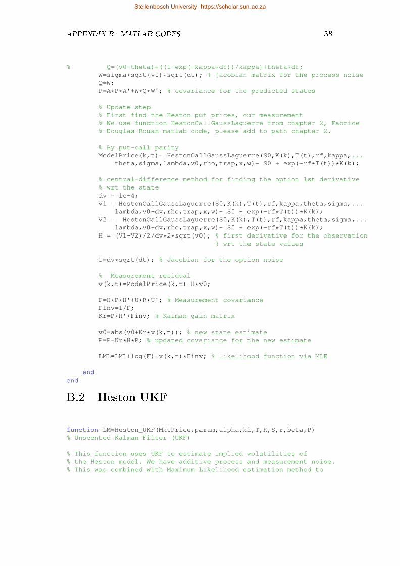
APPENDIX B. MATLAB CODES 58
% Q=(v0-theta)*((1-exp(-kappa*dt))/kappa)+theta*dt;W=sigma*sqrt(v0)*sqrt(dt); % jacobian matrix for the process noiseQ=W;P=A*P*A'+W*Q*W'; % covariance for the predicted states
% Update step% First find the Heston put prices, our measurement% We use function HestonCallGaussLaguerre from chapter 2, Fabrice% Douglas Rouah matlab code, please add to path chapter 2.
% By put-call parityModelPrice(k,t)= HestonCallGaussLaguerre(S0,K(k),T(t),rf,kappa,...
theta,sigma,lambda,v0,rho,trap,x,w)- S0 + exp(-rf*T(t))*K(k);
% central-difference method for finding the option 1st derivative% wrt the statedv = 1e-4;V1 = HestonCallGaussLaguerre(S0,K(k),T(t),rf,kappa,theta,sigma,...
lambda,v0+dv,rho,trap,x,w)- S0 + exp(-rf*T(t))*K(k);V2 = HestonCallGaussLaguerre(S0,K(k),T(t),rf,kappa,theta,sigma,...
lambda,v0-dv,rho,trap,x,w)- S0 + exp(-rf*T(t))*K(k);H = (V1-V2)/2/dv*2*sqrt(v0); % first derivative for the observation
% wrt the state values
U=dv*sqrt(dt); % Jacobian for the option noise
% Measurement residualv(k,t)=ModelPrice(k,t)-H*v0;
F=H*P*H'+U*R*U'; % Measurement covarianceFinv=1/F;Kr=P*H'*Finv; % Kalman gain matrix
v0=abs(v0+Kr*v(k,t)); % new state estimateP=P-Kr*H*P; % updated covariance for the new estimate
LML=LML+log(F)+v(k,t)*Finv; % likelihood function via MLE
endend
B.2 Heston UKF
function LM=Heston_UKF(MktPrice,param,alpha,ki,T,K,S,r,beta,P)% Unscented Kalman Filter (UKF)
% This function uses UKF to estimate implied volatilities of% the Heston model. We have additive process and measurement noise.% This was combined with Maximum Likelihood estimation method to
Stellenbosch University https://scholar.sun.ac.za
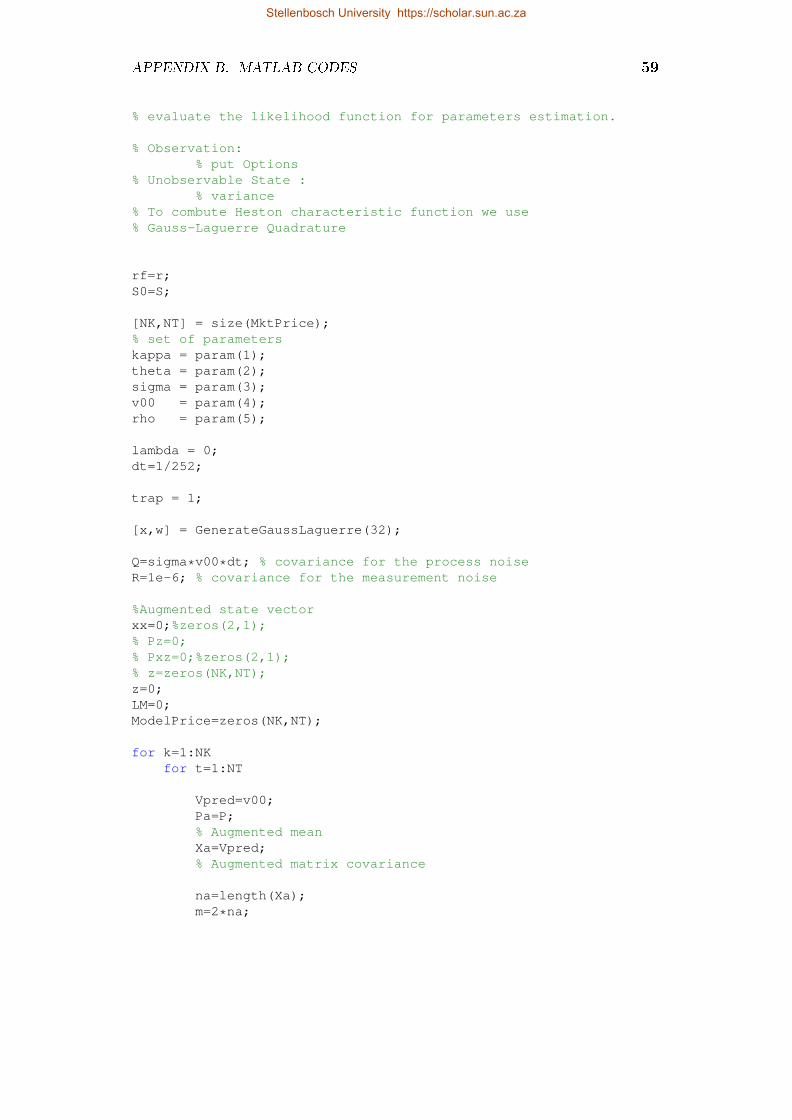
APPENDIX B. MATLAB CODES 59
% evaluate the likelihood function for parameters estimation.
% Observation:% put Options
% Unobservable State :% variance
% To combute Heston characteristic function we use% Gauss-Laguerre Quadrature
rf=r;S0=S;
[NK,NT] = size(MktPrice);% set of parameterskappa = param(1);theta = param(2);sigma = param(3);v00 = param(4);rho = param(5);
lambda = 0;dt=1/252;
trap = 1;
[x,w] = GenerateGaussLaguerre(32);
Q=sigma*v00*dt; % covariance for the process noiseR=1e-6; % covariance for the measurement noise
%Augmented state vectorxx=0;%zeros(2,1);% Pz=0;% Pxz=0;%zeros(2,1);% z=zeros(NK,NT);z=0;LM=0;ModelPrice=zeros(NK,NT);
for k=1:NKfor t=1:NT
Vpred=v00;Pa=P;% Augmented meanXa=Vpred;% Augmented matrix covariance
na=length(Xa);m=2*na;
Stellenbosch University https://scholar.sun.ac.za

APPENDIX B. MATLAB CODES 60
% Sigma points% alpha=1e-3;%0.99; %alpha is recommended to be between 10e-3 and 1% ki=0;% beta=2;
lambdaa=alpha*alpha*(na+ki)-na;
PO=sqrt((na+lambdaa)*real(Pa));
Xb=Xa;
Wm=zeros(1,m+1);Wc=zeros(1,m+1);for i=1:m+1
% Weightsif i~=1
Wm(i)=1/(2*(na+lambdaa));Wc(i)=1/(2*(na+lambdaa));
elseWm(i)=lambdaa/(na+lambdaa);Wc(i)=(lambdaa/(na+lambdaa))+(1-alpha*alpha+beta);
end%
if i==naXc(i)=Xa+PO;
elseXc(i)=Xa-PO;
end%
Xi=[Xb Xa+PO Xa-PO]; % set of sigma points% f=zeros(2,m+1);
% Prediction stepf=Xi(1,i)+kappa*(theta-Xi(1,i))*dt;%+Xi(2,i); %propagate sigma points
xx=xx+Wm(i)*f; % estimated meanP=((f-xx)*Wc(i)*(f-xx)) + Q; % prior covariance
% Update step
% Put option prices via Gauss-Laguerre QuadratureModelPrice(k,t) = HestonCallGaussLaguerre(S0,K(k),T(t),rf,kappa,...
theta,sigma,lambda,xx,rho,trap,x,w) - S0 + exp(-rf*T(t))*K(k);% put price, using% put-call parity.
z=z+Wm(i)*ModelPrice(k,t);zz=ModelPrice(k,t)-z;Pz=zz*Wc(i)*zz+R;Pxz=(f-xx)*Wc(i)*zz;
end
Stellenbosch University https://scholar.sun.ac.za

APPENDIX B. MATLAB CODES 61
% Kalman gainKr=Pxz/Pz;
% new estimatev00=abs(xx+Kr*(zz));P=P-Kr*Pz*Kr;
loglik=log(Pz)+(MktPrice(k,t)-z)/Pz;
% loglik=(-NK/2)*log(2*pi)-0.5*log(Pz)-0.5*(MktPrice(k,t)-z)*(MktPrice(k,t)-z)/Pz;
LM=LM+loglik; % likelihood function
endend
B.3 Heston PF
function LM = Heston_PF(MktPrice,param,N,K,T,S,r)% Particle Filtering (PF)% This function uses PF to estimate implied volatilities of% the Heston model.% This was combined with Maximum Likelihood estimation method to% evaluate the likelihood function for parameters estimation.
% Unobservable State :% variance
% To combute Heston characteristic function, we use% Gauss-Laguerre Quadrature% N=Number of Particles
kappa = param(1);theta = param(2);sigma = param(3);v0 = param(4);rho = param(5);
lambda = 0;
trap = 1;
[x,w] = GenerateGaussLaguerre(32);
rf=r;S0=S;q = 0.0068;dt=1/252;
Stellenbosch University https://scholar.sun.ac.za

APPENDIX B. MATLAB CODES 62
[NK,NT] = size(MktPrice);
LM=0;
xx=v0;
% Particle filterX = xx *ones(1,N);
for j=1:Nfor k=1:NK
for t=1:NT
xPred=xx;Q = (theta*sqrt(1-rho^2)*sqrt(xPred*dt))^2 + 1e-9;
% Sampling stepX=X+sqrtm(Q)*randn(1,N);
% Prediction stepX = X+kappa*(theta-X)*dt;X=abs(X);
% Put option via Gauss-Laguerre Quadrature of Heston% Characteristic func.
ModelPrice(k,t,j) = HestonCallGaussLaguerre(S0,K(k),T(t),rf,kappa,...theta,sigma,lambda,X(j),rho,trap,x,w) - S0 + exp(-rf*T(t))*K(k);
y(:,:,j)=ModelPrice(k,t,j);R = (xx*dt)+ 1e-9;
ww=exp(-0.5*y(:,:,j)'*inv(R)*y(:,:,j))+1e-15; %particles weight
ww=ww/sum(ww); % normalize the weights
yMean=sum(ww.*ModelPrice(k,t),1); % predicted measurements
xx=sum(ww.*X); % state estimatePP=ModelPrice(k,t)-yMean;P = (PP*diag(ww)*PP')+R; % measurement Cov
% Measurement ResidualMR = ModelPrice(k,t)-yMean;% LikelihoodLM=LM+0.5*log(det(P))+0.5*MR'*inv(P)*MR;
% Resampling stepNewIndex = Resample(ww);
X(:)=X(NewIndex);
Stellenbosch University https://scholar.sun.ac.za

APPENDIX B. MATLAB CODES 63
endend
endend
function NewIndex = Resample(ww)% This function Resample(ww) is taken from Mastro book, Chap: 9% Resample resamples [OldIndex=1:NumParticles; OldWeights=w]% to [NewIndex ; NewWeights=1/NumPart.,...,1/NumPart.]% e.g., NewIndex = [1 1 4 5 5 6 6 6 6]% Excellent comparison of resampling schemes available from% Nando de Freitas (Berkeley) and Rudolph van der Merwe (OGI)
L=max(size(ww));OldIndex=1:L;NewPart=zeros(1,L);CDFunc=cumsum(ww);
u = sort(rand(1,L));% Nando de Freitas and Rudolph van der Merwe suggest% u=fliplr(cumprod(rand(1,L).^(1./(L:-1:1))));j=1;for counter=1:L
while(u(counter) > CDFunc(j))j=j+1;
endNewPart(j)=NewPart(j)+1;
end
ind=1;for counter=1:L
if (NewPart(1,counter)>0)for j=ind:ind+NewPart(counter)-1
NewIndex(j) = OldIndex(counter);end
endind=ind+NewPart(counter);
endend
B.4 Double Heston EKF
function likelihood=EKFDH(MktPrice,param,K,T,S,r)% Extendend Kalman Filter(EKF) for the Double Heston model% This function uses EKF to estimate implied volatilities of the% Double Heston model.% This was combined with Maximum Likelihood estimation method to% evaluate the likelihood function for parameters estimation.
% Inputs:
Stellenbosch University https://scholar.sun.ac.za

APPENDIX B. MATLAB CODES 64
% K is the strike price% S is the stock price% T is maturity time% rf is the risk-free rate% q = dividend yield-rate% param = Two sets of Double Heston parameters% [kappa1 theta1 sigma1 v01 rho1,kappa2 theta2 sigma2 v02 rho2]% V01 and V02= the state transition equations% V01=v01+kappa1*(theta1-v01)*dt+noise% V02=v02+kappa2*(theta2-v02)*dt+noise;
% ModelPrice=observations, which is the put prices from double Heston% ModelPrice=DoubleHestonPriceGaussLaguerre(P,S,K(k),T(t),rf,q,param,x,w,trap);
rf=r;q = 0.0068;PutCall = 'P';[NK,NT] = size(MktPrice);
likelihood=0;
% Read in the weights and abscissas[x,w] = GenerateGaussLaguerre(32);
kappa1 = param(1); theta1 = param(2); sigma1 = param(3); v01= param(4);rho1 = param(5);kappa2 = param(6); theta2 = param(7); sigma2 = param(8); v02= param(9);rho2 = param(10);
dt=1/252;P1=0.03; % initial covarianceP2=0.02;v00=[v01 v02]';R=0.005536; % covariance matrix for the measurement noisesModelPrice=zeros(NK,NT);v=zeros(NK,NT);% "Little Trap, trap=1" formulation for the Heston characteristic functiontrap = 1;for t=1:NT %NT=4
for k=1:NK %NK=13Vpred=v00;if k==1
P=[P1 0; 0 P2];else
P=P;end
% prediction step
V=[Vpred(1,1)+kappa1*(theta1-Vpred(1,1))*dt; Vpred(2,1)+kappa2*...
Stellenbosch University https://scholar.sun.ac.za

APPENDIX B. MATLAB CODES 65
(theta2-Vpred(2,1))*dt]; % prediction of the states%(v02-theta2)*exp(-kappa2*dt)+theta2; % prediction of the states
% covariance matrix for the process noisesQ=[sigma1*Vpred(1,1)*dt 0;0 sigma2*Vpred(2,1)*dt];
% 1st derivative for the transtion wrt statesA=[1-kappa1*dt 0; 0 1-kappa2*dt];
W=[sigma1*sqrt(Vpred(1,1))*sqrt(dt) 0; 0 sigma2*sqrt(Vpred(2,1))*...sqrt(dt)]; % jacobian matrix for the process noise
P=A*P*A'+W*Q*W'; % covariance for the predicted process
% observations prices% this function was borrowed from chapter 12 in Fabrice% Douglas Rouah matlab code, please add to path chapter 12param(4)=Vpred(1,1); % assign new value of v01param(9)=Vpred(2,1); % assign new value of v02
ModelPrice(k,t) = DoubleHestonPriceGaussLaguerre(PutCall,S,K(k),...T(t),rf,q,param,x,w,trap);
% Perform Jacobian% central-difference methoddv = 1e-2;param(4)=Vpred(1,1)+dv;V01 = DoubleHestonPriceGaussLaguerre(PutCall,S,K(k),T(t),rf,q,param....
,x,w,trap);param(4)=Vpred(1,1)-2*dv;V02 = DoubleHestonPriceGaussLaguerre(PutCall,S,K(k),T(t),rf,q,param....
,x,w,trap);
param(4)=Vpred(1,1)+dv;
param(9)=Vpred(2,1)+dv;V11=DoubleHestonPriceGaussLaguerre(PutCall,S,K(k),T(t),rf,q,param,...
x,w,trap);param(9)=Vpred(2,1)-2*dv;V12 = DoubleHestonPriceGaussLaguerre(PutCall,S,K(k),T(t),rf,q,...
param,x,w,trap);
param(9)=Vpred(2,1)+dv;
% first derivative for the observation wrt the state valuesH1 = (V01-V02)/2/dv*2*sqrt(Vpred(1,1));H2 = (V11-V12)/2/dv*2*sqrt(Vpred(2,1));H=[H1 H2];U=[dv*sqrt(dt) dv*sqrt(dt)];% Jacobian for the option noise, which
%is assumed to be the same for both v01 and v02
% update step
Stellenbosch University https://scholar.sun.ac.za

APPENDIX B. MATLAB CODES 66
% Measurement residualv(k,t)=ModelPrice(k,t)-H*V;
F=H*P*H'+U.*R*U'; % Measurement covariance
Finv=inv(F);
Kr=P*H'.*Finv; % Kalman gain matrix
v00=abs(V+Kr.*v(k,t)); % new states
P=P-Kr*H*P; % updated covariance for the new estimated states
% Likelihood functionlikelihood=likelihood+log(F)+v(k,t)*Finv;
end
end
B.5 Double Heston UKF
function LM=Double_UKF(MktPrice,param,alpha,ki,T,K,S,r,beta)
% This function uses UKF to estimate implied volatilities of% the Double Heston model. There is additive process and measurement noise.% This was combined with Maximum Likelihood estimation method to% evaluate the likelihood function for parameters estimation.% Observation:
% put Options% Unobservable State :
% variance% To compute double Heston characteristic function, we use% Gauss-Laguerre Quadrature
rf=r;S0=S;q = 0.0068;PutCall = 'P';[NK,NT] = size(MktPrice);% set of parameterskappa1 = param(1); theta1 = param(2); sigma1 = param(3); v01= param(4);rho1 = param(5);kappa2 = param(6); theta2 = param(7); sigma2 = param(8); v02= param(9);rho2 = param(10);
dt=1/252;
trap = 1;
Stellenbosch University https://scholar.sun.ac.za

APPENDIX B. MATLAB CODES 67
[x,w] = GenerateGaussLaguerre(32);
%Augmented state vectorxx=zeros(2,1);v00=[v01 v02]';% Pz=0;% Pxz=0;%zeros(2,1);% z=zeros(NK,NT);z=0;LM=0;ModelPrice=zeros(NK,NT);
for k=1:NKfor t=1:NT
Vpred=v00;if t==1
Pa=[rho1 0; 1 rho2];else
Pa=P;end
% Augmented meanXa=Vpred;% Augmented matrix covariance
na=length(Xa); % 2x1m=2*na; % 4
% Sigma points% alpha=1e-3;%0.99; %alpha is recommended to be between 10e-3 and 1% ki=0;% beta=2;
lambdaa=alpha*alpha*(na+ki)-na;
PO=sqrt((na+lambdaa).*real(Pa));
Xb=Xa;
Wm=zeros(1,m+1);Wc=zeros(1,m+1);for i=1:m+1
% Weightsif i~=1
Wm(i)=1/(2*(na+lambdaa));Wc(i)=1/(2*(na+lambdaa));
elseWm(i)=lambdaa/(na+lambdaa);Wc(i)=(lambdaa/(na+lambdaa))+(1-alpha*alpha+beta);
Stellenbosch University https://scholar.sun.ac.za

APPENDIX B. MATLAB CODES 68
end
Xc=zeros(na,2*na);for j=1:na
Xc(:,j)=Xa+PO(:,j);endfor j=na+1:m
Xc(:,j)=Xa-PO(:,j-na);end
Xi=[Xb Xc]; % set of sigma points
% f=zeros(2,m+1);% Prediction step
f=[Xi(1,i)+kappa1*(theta1-Xi(1,i))*dt;Xi(2,i)+kappa2*...(theta2-Xi(2,i))*dt];
xx=xx+Wm(i).*f; % predicted statesP=Wc(i).*(f-xx)*(f-xx)' ; % predicted state covariance
param(4)=xx(1,1);param(9)=xx(2,1);
% Put option prices via Gauss-Laguerre QuadratureModelPrice(k,t) = DoubleHestonPriceGaussLaguerre(PutCall,S,K(k),T(t),rf,q,param,x,w,trap);
z=z+Wm(i)*ModelPrice(k,t); % prediction of observationszz=ModelPrice(k,t)-z;Pz=zz*Wc(i)*zz; % predicted observations covariancePxz=(f-xx)*Wc(i)*zz; % joint covarinace of state and observation
end
% Update step
% Kalman gainKr=Pxz/Pz; % 2x1
% new state estimatev00=abs(xx+Kr.*(zz));P=P-Kr*Pz*Kr'; % state covariance
loglik=log(Pz)+(MktPrice(k,t)-z)/Pz;
%loglik=(-NK/2)*log(2*pi)-0.5*log(Pz)-0.5*(MktPrice(k,t)-z)*(MktPrice(k,t)-z)/Pz;
LM=LM+loglik; % likelihood function
endend
Stellenbosch University https://scholar.sun.ac.za

APPENDIX B. MATLAB CODES 69
B.6 Double Heston PF
function LM = Double_PF(MktPrice,param,N,K,T,S,r)% Particle Filtering for the Double Heston model
% This function uses PF to estimate implied volatilities of% the Double Heston model. We have additive process and measurement noise.% This was combined with Maximum Likelihood estimation method to% evaluate the likelihood function for parameters estimation.
% Observation:% put Options
% Unobservable State :% variance
% To compute double Heston characteristic function, we use% Gauss-Laguerre Quadrature% N=Number of Particles
kappa1 = param(1); theta1 = param(2); sigma1 = param(3);v01= param(4); rho1 = param(5); kappa2 = param(6);theta2 = param(7); sigma2 = param(8); v02= param(9);rho2 = param(10);
lambda = 0;
trap = 1;
[x,w] = GenerateGaussLaguerre(32);
% Initialize Process CovariancePxx=[rho1 0; 1 rho2];
rf=r;S0=S;q = 0.0068;dt=1/252;[NK,NT] = size(MktPrice);PutCall = 'P';LM=0; %0.5*nSteps*log(2*pi);
xx=[v01 v02]';
X = xx *ones(1,N);
for j=1:Nfor k=1:NK
for t=1:NT
xPred=xx;
Stellenbosch University https://scholar.sun.ac.za

APPENDIX B. MATLAB CODES 70
Q=[sigma1*xPred(1,1)*dt 0;0 sigma2*xPred(2,1)*dt];
% Sampling stepX=X+sqrtm(Q)*randn(2,N);
% Prediction stepX = X+([kappa1*(theta1-X(1,:)); kappa2*(theta2-X(2,:))])*dt;X=abs(X);
% Put option via Gauss-Laguerre Quadrature of Heston Characteristic func.
param(4)=X(1,j);param(9)=X(2,j);
ModelPrice(k,t,j) = DoubleHestonPriceGaussLaguerre(PutCall,...S,K(k),T(t),rf,q,param,x,w,trap);
y(:,:,j)=ModelPrice(k,t,j);R = diag(xPred*sqrt(dt))';
% particle weightww=exp(-0.5*y(:,:,j)'*inv(R)*y(:,:,j))+1e-15;
ww=ww/sum(ww); % normalize the weights
yMean=sum(ww.*ModelPrice(k,t),1);
xx=[sum(ww(1,1).*X(1,j)) sum(ww(2,1).*X(2,j))]';PP=ModelPrice(k,t)-yMean;P= (PP*diag(ww)*PP')+R; % measurement covariance
% Measurement ResidualMR = ModelPrice(k,t)-yMean; % option price error% Likelihood functionLM=LM+sum(sum(0.5*log(det(Pyy))+0.5*MR'*inv(Pyy)*MR));
% Resampling stepNewIndex = Resample(ww);
X(:,j)=X(NewIndex);
endend
endend
Stellenbosch University https://scholar.sun.ac.za

List of References
Albrecher, H., Mayer, P., Schoutens, W. and Tistaert, J. (2006). The little hestontrap.
Albrecher, H., Mayer, P. and Schoutens, W.T. (2007). The little heston trap. Wilmott
Magazine, January issue, pp. 8392.
Andersen, T.G., Benzoni, L. and Lund, J. (2002). An empirical investigation ofcontinuous-time equity return models. The Journal of Finance, vol. 57, no. 3, pp.12391284.
Andersen, T.G. and Bollerslev, T. (1997). Heterogeneous information arrivals andreturn volatility dynamics: Uncovering the long-run in high frequency returns.The Journal of Finance, vol. 52, no. 3, pp. 9751005.
Arulampalam, M.S., Maskell, S., Gordon, N. and Clapp, T. (2002). A tutorial onparticle lters for online nonlinear/non-gaussian bayesian tracking. Signal Pro-
cessing, IEEE Transactions on, vol. 50, no. 2, pp. 174188.
Bakshi, G., Cao, C. and Chen, Z. (1997). Empirical performance of alternativeoption pricing models. The Journal of Finance, vol. 52, no. 5, pp. 20032049.
Ball, C.A. and Roma, A. (1994). Stochastic volatility option pricing. Journal of
Financial and Quantitative Analysis, vol. 29, no. 04, pp. 589607.
Bollerslev, T. (1986). Generalized autoregressive conditional heteroskedasticity.Journal of Econometrics, vol. 31, no. 3, pp. 307327.
Chernov, M. and Ghysels, E. (2000). A study towards a unied approach to thejoint estimation of objective and risk neutral measures for the purpose of optionsvaluation. Journal of nancial economics, vol. 56, no. 3, pp. 407458.
Christoersen, P., Heston, S. and Jacobs, K. (2009). The shape and term structureof the index option smirk: Why multifactor stochastic volatility models work sowell. Management Science, vol. 55, no. 12, pp. 19141932.
Christoersen, P. and Jacobs, K. (2004). The importance of the loss function inoption valuation. Journal of Financial Economics, vol. 72, no. 2, pp. 291318.
Christoersen, P., Jacobs, K. and Mimouni, K. (2010). Volatility dynamics for thes&p500: evidence from realized volatility, daily returns, and option prices. Reviewof Financial Studies, vol. 23, no. 8, pp. 31413189.
71
Stellenbosch University https://scholar.sun.ac.za

LIST OF REFERENCES 72
Costabile, M., Massabo, I. and Russo, E. (2012). On pricing contingent claimsunder the double heston model. International Journal of Theoretical and Applied
Finance, vol. 15, no. 05.
Doucet, A., De Freitas, N., Murphy, K. and Russell, S. (2000). Rao-blackwellisedparticle ltering for dynamic bayesian networks. In: Proceedings of the Sixteenthconference on Uncertainty in articial intelligence, pp. 176183. Morgan Kauf-mann Publishers Inc.
Due, D., Pan, J. and Singleton, K. (2000). Transform analysis and asset pricingfor ane jump-diusions. Econometrica, vol. 68, no. 6, pp. 13431376.
Engle, R.F. (1982). Autoregressive conditional heteroscedasticity with estimates ofthe variance of united kingdom ination. Econometrica: Journal of the Econo-
metric Society, pp. 9871007.
Gouriéroux, C. (2012). ARCH models and nancial applications. Springer Science& Business Media.
Guo, B., Han, Q. and Zhao, B. (2014). The nelsonsiegel model of the term structureof option implied volatility and volatility components. Journal of Futures Markets,vol. 34, no. 8, pp. 788806.
Hermann, R. and Krener, A.J. (1977). Nonlinear controllability and observability.IEEE Transactions on automatic control, vol. 22, no. 5, pp. 728740.
Heston, S.L. (1993). A closed-form solution for options with stochastic volatility withapplications to bond and currency options. Review of Financial Studies, vol. 6,no. 2, pp. 327343.
Hol, J.D., Schon, T.B. and Gustafsson, F. (2006). On resampling algorithms forparticle lters. In: Nonlinear Statistical Signal Processing Workshop, 2006 IEEE,pp. 7982. IEEE.
Hull, J. and White, A. (1987). The pricing of options on assets with stochasticvolatilities. The Journal of Finance, vol. 42, no. 2, pp. 281300.
Hurn, A.S., Lindsay, K.A. and McClelland, A.J. (2015). Estimating the parametersof stochastic volatility models using option price data. Journal of Business &
Economic Statistics, vol. 33, no. 4, pp. 579594.
Javaheri, A. (2011). Inside volatility arbitrage: the secrets of skewness, vol. 317. JohnWiley & Sons.
Javaheri, A., Lautier, D. and Galli, A. (2003). Filtering in nance. Wilmott, vol. 3,pp. 6783.
Julier, S.J. and Uhlmann, J.K. (1996). A general method for approximating nonlineartransformations of probability distributions. Tech. Rep., Technical Report, RRG,Department of Engineering Science, University of Oxford.
Stellenbosch University https://scholar.sun.ac.za

LIST OF REFERENCES 73
Kalman, R.E. (1960). A new approach to linear ltering and prediction problems.Journal of Fluids Engineering, vol. 82, no. 1, pp. 3545.
Kienitz, J. and Wetterau, D. (2012). Financial modelling: Theory, implementationand practice with matlab source. John Wiley & Sons.
Lagarias, J.C., Reeds, J.A., Wright, M.H. and Wright, P.E. (1998). Convergenceproperties of the neldermead simplex method in low dimensions. SIAM Journal
on optimization, vol. 9, no. 1, pp. 112147.
Li, J. (2013). An unscented kalman smoother for volatility extraction: Evidencefrom stock prices and options. Computational Statistics & Data Analysis, vol. 58,pp. 1526.
Lu, L., Yang, M., Geng, S., Wang, S.-f. and Wang, Y.-h. (2015). Study on importancefunction for particle lter. International Journal of Multimedia and Ubiquitous
Engineering, vol. 10, no. 2, pp. 249258.
Nason, J.M. and Smith, G. (2013). Reverse kalman ltering us ination with stickyprofessional forecasts.
Pan, J. (2002). The jump-risk premia implicit in options: Evidence from an inte-grated time-series study. Journal of nancial economics, vol. 63, no. 1, pp. 350.
Reif, K., Günther, S., Yaz, E. and Unbehauen, R. (1999). Stochastic stability of thediscrete-time extended kalman lter. IEEE Transactions on Automatic Control,vol. 44, no. 4, pp. 714728.
Rouah, F.D. (2013). The Heston model and its extensions in MATLAB and C#.John Wiley & Sons.
Rouah, F.D. (2013 (accessed September 3, 2015)). The heston model and its exten-sions in matlab and c#.Available at: http://eu.wiley.com/WileyCDA/Section/id-818210.html
Scott, L.O. (1987). Option pricing when the variance changes randomly: Theory,estimation, and an application. Journal of Financial and Quantitative Analysis,vol. 22, no. 04, pp. 419438.
Shephard, N. (2005). Stochastic volatility. Economics Group, Nueld College, Uni-
versity of Oxford, Economics Papers.
Sira-Ramirez, H. (1988). Algebraic condition for observability of non-linear analyticsystems. International Journal of Systems Science, vol. 19, no. 11, pp. 21472155.
Stein, E.M. and Stein, J.C. (1991). Stock price distributions with stochastic volatil-ity: an analytic approach. Review of nancial Studies, vol. 4, no. 4, pp. 727752.
Tanizaki, H. (2013). Nonlinear lters: estimation and applications. Springer Science& Business Media.
Stellenbosch University https://scholar.sun.ac.za
LIST OF REFERENCES 74
Théoret, R. and Racicot, F.-É. (2010). Forecasting stochastic volatility using thekalman lter: An application to canadian interest rates and price-earnings ratio.
Thrun, S. (2002). Particle lters in robotics. In: Proceedings of the Eighteenth con-
ference on Uncertainty in articial intelligence, pp. 511518. Morgan KaufmannPublishers Inc.
Van Der Merwe, R., Doucet, A., De Freitas, N. and Wan, E. (2000). The unscentedparticle lter. In: NIPS, vol. 2000, pp. 584590.
Wan, E.A. and Van Der Merwe, R. (2000). The unscented kalman lter for nonlinearestimation. In: Adaptive Systems for Signal Processing, Communications, and
Control Symposium 2000. AS-SPCC. The IEEE 2000, pp. 153158. Ieee.
Zhu, J. (2009). Applications of Fourier transform to smile modeling: Theory and
implementation. Springer Science & Business Media.
Stellenbosch University https://scholar.sun.ac.za