Volatility Risk and the Pricing Kernel in the Heston and ... · The Pricing Kernel in the Heston and Nandi (2000) and Heston ... the idea of pricing kernel is originally implicit

The Pricing Kernel in the Heston and Nandi (2000) and Heston

(1993) Index Option Pricing Model: An Empirical Puzzle

Qi Sun

A Thesis

in

The John Molson School

of

Business

Presented in Partial Fulfillment of the Requirements for the

Degree of Master of Science at Concordia University

Montreal, Quebec, Canada

October 2014

© Qi Sun, 2014

CONCORDIA UNIVERSITY

School of Graduate Studies

This is to certify that the thesis prepared

By: Qi Sun

Entitled: The Pricing Kernel in the Heston and Nandi (2000) and Heston (1993) Index

Option Pricing Model: An Empirical Puzzle

and submitted in partial fulfillment of the requirements for degree of

Master of Science (Finance)

complies with the regulations of the University and meets the accepted standards with respect to

originality and quality.

Signed by the final Examining Committee:

Chair

Dr. A. Dawson

Examiner

Dr. L. Switzer

Examiner

Dr. O. Taperio

Supervisor

Dr. S. Perrakis

Approved by C

Chair of Department or Graduate Program Director

2014 r

Dean of Faculty

iii

Abstract

The Pricing Kernel in the Heston and Nandi (2000) and Heston (1993)

Index Option Pricing Model: An Empirical Puzzle

Qi Sun

This thesis estimates a quadratic pricing kernel developed by Christoffersen, Heston and Jacobs

(2013) under the Heston-Nandi GARCH pricing model, using both American and Canadian data.

Initially, we find a misfit of data across different data samples, indicating lack of support in the

closed-form quadratic pricing kernel. Comparing with the estimation of the continuous-time

Heston (1993) model from Christoffersen, Jacobs, and Mimouni (2010), this empirical puzzle

exists in both the Heston-Nandi (2000) GARCH and Heston (1993) stochastic volatility model.

We provide additional tests by comparing the Heston-Nandi and CHJ model with the

overreaction tests. We find that their empirical performances are not differentiated. Also, we

introduce the stochastic dominance bounds in order to select the mispriced options. The results

from filtered data sample indicate the mispricing of options is significantly affecting the

estimation.

iv

Acknowledgements

I would like to thank my thesis supervisor Professor Stylianos Perrakis.

v

Table of Contents

Abstract .......................................................................................................................................... iii

Acknowledgements ........................................................................................................................ iv

Table of Contents ............................................................................................................................ v

List of Tables ................................................................................................................................. vi

1 Introduction .............................................................................................................................. 1

2 The Pricing Kernel ................................................................................................................... 7

2.1 Introduction ......................................................................................................................... 7

2.2 The Heston-Nandi GARCH Model ..................................................................................... 8

2.3 GARCH Pricing Kernel .................................................................................................... 10

3 Estimation .............................................................................................................................. 13

3.1 Data ................................................................................................................................... 13

3.2 Joint Likelihood Estimation .............................................................................................. 17

4 The Overreaction Test ........................................................................................................... 24

5 Stochastic Dominance Bounds .............................................................................................. 28

5.1 Introduction ....................................................................................................................... 28

5.2 Estimation ......................................................................................................................... 28

6 The Continuous-Time Heston Model .................................................................................... 34

7 Concluding Remarks.............................................................................................................. 37

Reference ...................................................................................................................................... 38

Appendix ....................................................................................................................................... 42

vi

List of Tables

3.1 Dow Jones Industrial Average index and options data description .................................. 15

3.2 S&P TSX 60 index and options data description .............................................................. 16

3.3 Joint maximum likelihood estimation with Dow Jones Industrial Average index and

options ........................................................................................................................................... 19

3.4 Joint maximum likelihood estimation with S&P TSX 60 index and options ................... 20

3.5 Joint maximum likelihood estimation with S&P 500 index and options .......................... 21

4.1 Long-term volatility overreaction tests ............................................................................. 26

5.1 Joint maximum likelihood estimation with S&P 500 index and 1-month call options .... 31

5.2 Joint maximum likelihood estimation with S&P 500 index and 1-month call options

filtered by the stochastic dominance bounds ................................................................................ 32

1

1 Introduction

The merits of the Black-Scholes model have been widely accepted among academics and

investment professionals. It assumes a complete and perfect market that provides a continuous

path of the underlying security and a constant variance of the stock return, while the asset price

follows a geometric Brownian motion. The assumption establishes a unique framework of risk-

neutral probability measure. Also, the idea of pricing kernel is originally implicit in the theory of

Black and Scholes (1973) since the absence of arbitrage implies a positive stochastic discount

factor. Motivated by the intuitions from the Black-Scholes model, a voluminous option pricing

literature has developed on the studies of risk-neutral measurement and pricing kernel.

However, many systematic deviations from the Black-Scholes model remain unexplained. The

original assumption of lognormal distribution of asset price presented by Black-Scholes has been

challenged after the 1987-crash. In addition, the variance of returns on assets tends to be unstable

over time. Furthermore, the realized volatilities are systematically and consistently lower than at-

the-money (ATM) implied volatilities. There have been two directions of modeling such a

feature of the data. The first one is stochastic volatility. Many option pricing models have been

focusing on parametric continuous-time models for the underlying asset. The unsatisfactory

performance of the constant variance geometric Brownian motion leads to a new class of the

stochastic volatility models. These models assume that volatility is volatile itself and moving

towards a long-term mean.

Originating with Garman (1976), stochastic volatility (SV) option pricing models have to satisfy

a fundamental partial differential equation (PDE) of both underlying price and volatility. The

early SV models have the most general solutions of the PDEs but they are infeasible to compute.

Both Hull and White (1987) and Stein and Stein (1991) have problems in generating the

characteristic function of distribution of the average variance. Alternatively, Heston (1993)

develops a specific stochastic volatility diffusion. He computes the risk-neutral probabilities that

a call option will expire in-the-money (ITM) by a Fourier transform of a conditional

characteristic function, which is known in closed form under his assumption that stochastic

2

volatility follows a square-root diffusion. The option price is generated together with index and

strike prices. Building on this insight, numerous studies have been investigating the Heston-type

stochastic volatility model. Benzoni (1998) and Eraker, Johannes, and Polson (2003) conclude

that the SV model provides a much better fit of data than standard one-factor diffusions. In

particular, the Heston model contains a leverage effect, which allows an arbitrary correlation

between volatility and asset returns. It is consistent with the negative skewness observed in stock

returns. Also, the non-zero risk premium for volatility is indispensable to the closed-form

solution of the option prices; its inclusion is an important step towards the correction of

mispricing and the hedging errors for out-of-money options. The closed-form pricing model

from Heston (1993) is very influential.

The Heston model has been generalized to a rich class of affine jump-diffusion (AJD) by Duffie,

Pan, and Singleton (2000), who present the transform results for general affine models. The Cox,

Ingersoll, and Ross (CIR) model is also one of AJD models in the term structure literature. The

AJD approach models the asset price dynamics by means of introducing price-jumps, stochastic

volatility, and their combination. It is considered to be consistent with the empirical data and

many other specifications.

An alternative to the stochastic volatility model is the GARCH model. GARCH models have the

inherent advantage that volatility is observable; they are thus widely adopted. Following the

work of Engle (1982) and Bollerslev (1986), numerous econometric studies have been developed

on volatility estimation and forecasting. Bollerslev, Chou, and Kroner (1992) provide a thorough

overview of the GARCH literature and the empirical applications from a large class of the model.

Motivated by the success of GARCH models in estimating and forecasting volatility, researchers

have introduced the GARCH model into option valuation. Duan (1995) first proposes a

NGARCH (1, 1) 1 option valuation model, which assumes a locally risk-neutral valuation

relationship (LRNVR) to measure the return process by adjusting asset-specific drift terms under

the risk-neutral distribution. With LRNVR, Duan (1995) characterizes the transition between

1 NGARCH is introduced by Engle and Ng (1993).

3

physical and risk-neutral distributions under the GARCH framework. It implies that the

variances under both physical and risk-neutral measures are identical, corresponding to a linear

pricing kernel. After 50,000 Monte Carlo simulations, the model prices indicate that Black–

Scholes model underprices deep out-of-money options and short-maturity options. Duan and

Simonato (1998) further propose an empirical martingale simulation (EMS) method, which

ensures that the simulated option price satisfies rational price bounds. The EMS has a significant

effect on reducing the Monte Carlo errors.

Among most of the GARCH option pricing models, the main technical problem is the derivation

of the distribution of future asset prices (Stentoft, 2005). Numerical methods have to be applied

instead. An exception of this is the particular formulation in Heston and Nandi (2000). They

widely follow the concept of LRNVR and formulate a specific affine GARCH model that yields a

closed-form solution. The closed form is based on an inversion of the characteristic function

technique, which is introduced by Heston (1993), under the normal innovations. They also

provide considerable empirical supports to the Heston-Nandi model. It outperforms the ad-hoc

implied volatility benchmark model of Dumas, Fleming, and Whaley (1988) that use an

independent implied volatility for each option to fit the volatility smile. They conclude that the

improvements provided by their model are largely due to the inclusion of the leverage effect as

well as the path dependent in volatility. Their empirical results have brought GARCH option

pricing models to the forefront.

The importance of GARCH option pricing has expanded due to their linkage with stochastic

volatility models. Nelson (1990) is one of the first papers to examine the continuous-time limits

of GARCH models. Duan (1997) extends Nelson’s work into a broader class of GARCH models,

including NGARCH, EGARCH, GJR-GARCH, etc. Heston and Nandi (2000) document how the

Heston-Nandi model approaches the stochastic volatility model of Heston (1993) in the

continuous-time limit. The Heston-Nandi model is thus considered as a special case of the

Heston-type model. Both of them yield closed-form solutions, indicate the leverage effect, and

take advantage of the Fourier transform of the characteristic function. They also manage to

contain the volatility dynamics those capture the stylized facts in the option market. Based on all

the advantages, the Heston and Heston-Nandi models have been the most popular option pricing

4

models over the last two decades. Despite the great success achieved by the Heston and Heston-

Nandi model, they have not been evaluated in the context of the equilibrium theory with an

analytical pricing kernel.

Several equivalent martingale measures for option pricing models have been proposed and tested

so far. LRNVR from Duan (1995) is the first theoretical risk-neutralization for GARCH option

valuation. The conditional Esscher transform2 for option valuation, proposed by Gerber and Shiu

(1994), is also used for many applications. Building on the Esscher transform, Christoffersen,

Elkamhi, Feunou, and Jacobs (2010) characterize the Radon-Nikodym derivative for neutralizing

a class of GARCH models. Monfort and Pegoraro (2012) further propose a second-order Esscher

transform method. The pricing kernel for Heston and Heston-Nandi model is not developed in a

recent paper as Christoffersen, Heston, and Jacobs (2013, CHJ hereafter). CHJ (2013) propose a

closed-form variance-dependent pricing kernel for the Heston (1993) and also the Heston-Nandi

(2000) model. The pricing kernel accounts for both the equity premium and the variance risk

premium. The authors claim that the new parameters improve the explanatory power relative to

from several empirical phenomena. Specifically, in order to provide a unified explanation for the

empirical puzzles, they develop a conditional U-shaped relation between the conditional pricing

kernel and the returns, presented by a quadratic function of the market return. Moreover, they

solve the quantitative mappings between physical parameters and risk-neutral parameters. The

CHJ pricing kernel successfully models various empirical data, robust across multiple time

periods. In particular, CHJ introduce three types of stylized facts, including the U-shaped pricing

kernel, short-sell straddle strategy, and the implied volatility overreaction. The newly developed

quadratic pricing kernel is successful in capturing such stylized facts (see CHJ for more details).

However, despite the model’s advantages, CHJ (2013) have shown that a core parameter suffers

a parametric magnitude problem under the GARCH estimation. The risk-aversion parameter is

problematic and may lead to a failure of the CRRA marginal utility function. This would

invalidate the model, while the pricing kernel is no longer appropriately estimated.

2 Esscher transform is introduced by Esscher (1932).

5

The primary purpose of this paper is to further examine the quadratic pricing kernel under the

GARCH process and to compare it to the pricing kernel from Heston’s (1993) model. Since the

estimation is based on a multiple-dimensional joint-likelihood, which is highly sensitive due to

the information from both the return dynamics and the option prices, we attempt to determine

whether the misfit of data presented by the quadratic pricing kernel is a general case from

various option markets. Also, it is of great importance to compare the GARCH model estimation

with the stochastic volatility model estimation since they share the same pricing kernel. This

study corroborates these findings as the estimation problem is present in both American and

Canadian data. Moreover, our analysis suggests the newly developed pricing kernel under both

GARCH and stochastic volatility dynamics tends to have empirical puzzles.

We attempt to extract the cause of such a misfit of data. In a seminal paper, Jackwerth (2000)

documents massive changes of the pricing kernel during the 1987 crash. It is the famous “pricing

kernel puzzle”. A possible reason of the puzzle from Jackwerth is the mispricing of the options

in the market. Following Jackwerth (2000), it is natural for us to introduce the stochastic

dominance bounds to remove the mispriced options from our options sample. Intuitively, the

mispriced options are expected to violate such bounds and thus to provide noisy information with

respect to the model estimation.

The stochastic dominance bounds for the options prices are initially derived by Perrakis and

Ryan (1984), who use the Rubinstein (1976) procedure. This methodology is based on the single

price law and arbitrage arguments, which require the entire distribution. Perrakis (1986) and

Perrakis (1988) extend the Perrakis-Ryan bounds into a multiperiod context. On the other side,

the linear programming bounds, derived by Ritchken (1985), show an identical upper bound to

the Perrakis-Ryan upper bound. The Ryan bounds rely on market equilibrium arguments. It also

claims the lower bound of linear programming approach is tighter than that of Perrakis-Ryan

approach. The LP approach is extended to the multiperiod by Ritchken and Kuo (1988).

Following Perrakis and Ryan (1984), Constantinides and Perrakis (2002) derive the bounds with

intermediate trading of the underlying asset and proportional transaction costs. The derivations

are based on the multiperiod utility maximization with transaction costs originally from

6

Constantinides (1979). Constantinides, Jackwerth and Perrakis (2009) empirically examine the

S&P 500 options with the theory from Constantinides and Perrakis (2002). Constantinides and

Perrakis (2007) further extend the Constantinides-Perrakis bounds to American options.

In our study we identify mispriced 1-month S&P 500 call options using the Constantinides-

Perrakis bounds. In order to select the option data, a non-parametric form is imposed while

estimating the statistical distribution of the S&P 500 index returns through the kernel density

estimation. We then estimate the pricing kernels with option data filtered by the stochastic

dominance bounds. A significant influence from the mispriced options is well documented by

our empirical results.

The remainder of this paper is organized as follows. Section 2 analyzes the two types of pricing

kernels we test in the paper. Section 3 details the new methodology for fitting the GARCH

pricing kernels and presents the estimation results. Section 4 compares the linear and quadratic

pricing kernels from the implied volatility overreaction tests. Section 5 provides extensions on

the stochastic dominance bounds. Section 6 analyzes the empirical estimation of the continuous-

time Heston (1993) model and compares it to our discrete-time GARCH estimation. Section 7

concludes.

7

2 The Pricing Kernel

2.1 Introduction

In option pricing, the estimation of time-series volatility models using underlying returns yields

the physical distribution. On the other hand, the option prices extracted from the available market

option data lead to the risk-neutral or Q-distribution. The connection between these two

distributions is regarded as a central issue in options research. The stochastic discount factor or

pricing kernel, which is estimated by the ratio of risk-neutral to physical distribution, becomes an

essential component of such researches.

In a seminal paper Merton (1971) introduces a family of hyperbolic absolute risk aversion

(HARA) utility function, which indicates the risk tolerance as a linear function of the

consumption. The HARA-type utility functions are widely used in financial economics since

they include both constant (CRRA)3 and non-constant relative risk aversion. The study derives a

marginal utility function that corresponds to the optimal portfolio and consumption rules under

HARA. Rubinstein (1976) works further on the ideas of Merton and replicates the Black-Scholes

model with a particular pricing kernel by narrowing the type of utility to constant relative risk

aversion (CRRA):

𝑈𝑡(𝐶�̃�) = 𝜌1𝜌2 … 𝜌𝑡

1

1 − 𝑏𝐶�̃�

1−𝑏

where 𝜌𝑡 is a measure of time-preference. Following the CRRA utility function, the marginal

utility is:

𝑈𝑡′(𝐶�̃�) = 𝜌1𝜌2 … 𝜌𝑡𝐶�̃�

−𝑏

In standard financial models the pricing kernel is proportional to the marginal utility of a

representative investor. The asset prices are derived by a single decision problem of the

representative investor. The investors are assumed to be risk-averse and trade in a complete set

of markets from the model. As a result, the pricing kernel is a monotone decreasing function of

3 The standard CRRA utility function is given by u(𝑐) = 𝑐1−𝑏 (1 − 𝑏)⁄ with 𝑏 > 0. 𝑏 is the coefficient of

relative risk aversion and also the elasticity of marginal utility for consumption since 𝑏 = −𝑐u′′(𝑐) u′(𝑐)⁄ .

8

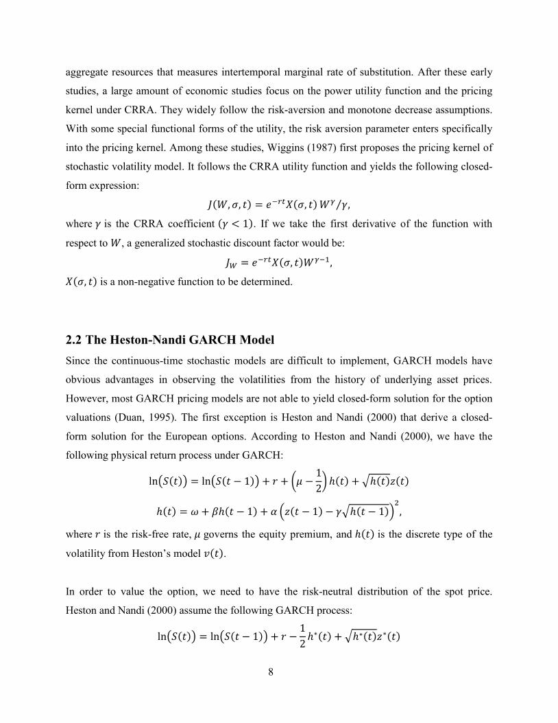
aggregate resources that measures intertemporal marginal rate of substitution. After these early

studies, a large amount of economic studies focus on the power utility function and the pricing

kernel under CRRA. They widely follow the risk-aversion and monotone decrease assumptions.

With some special functional forms of the utility, the risk aversion parameter enters specifically

into the pricing kernel. Among these studies, Wiggins (1987) first proposes the pricing kernel of

stochastic volatility model. It follows the CRRA utility function and yields the following closed-

form expression:

𝐽(𝑊, 𝜎, 𝑡) = 𝑒−𝑟𝑡𝑋(𝜎, 𝑡) 𝑊𝛾 𝛾⁄ ,

where 𝛾 is the CRRA coefficient (𝛾 < 1). If we take the first derivative of the function with

respect to 𝑊, a generalized stochastic discount factor would be:

𝐽𝑊 = 𝑒−𝑟𝑡𝑋(𝜎, 𝑡)𝑊𝛾−1,

𝑋(𝜎, 𝑡) is a non-negative function to be determined.

2.2 The Heston-Nandi GARCH Model

Since the continuous-time stochastic models are difficult to implement, GARCH models have

obvious advantages in observing the volatilities from the history of underlying asset prices.

However, most GARCH pricing models are not able to yield closed-form solution for the option

valuations (Duan, 1995). The first exception is Heston and Nandi (2000) that derive a closed-

form solution for the European options. According to Heston and Nandi (2000), we have the

following physical return process under GARCH:

ln(𝑆(𝑡)) = ln(𝑆(𝑡 − 1)) + 𝑟 + (𝜇 −1

2) ℎ(𝑡) + √ℎ(𝑡)𝑧(𝑡)

ℎ(𝑡) = 𝜔 + 𝛽ℎ(𝑡 − 1) + 𝛼 (𝑧(𝑡 − 1) − 𝛾√ℎ(𝑡 − 1))2

,

where 𝑟 is the risk-free rate, 𝜇 governs the equity premium, and ℎ(𝑡) is the discrete type of the

volatility from Heston’s model 𝑣(𝑡).

In order to value the option, we need to have the risk-neutral distribution of the spot price.

Heston and Nandi (2000) assume the following GARCH process:

ln(𝑆(𝑡)) = ln(𝑆(𝑡 − 1)) + 𝑟 −1

2ℎ∗(𝑡) + √ℎ∗(𝑡)𝑧∗(𝑡)

9

ℎ∗(𝑡) = 𝜔∗ + 𝛽ℎ∗(𝑡 − 1) + 𝛼∗ (𝑧∗(𝑡 − 1) − 𝛾∗√ℎ∗(𝑡 − 1))2

.

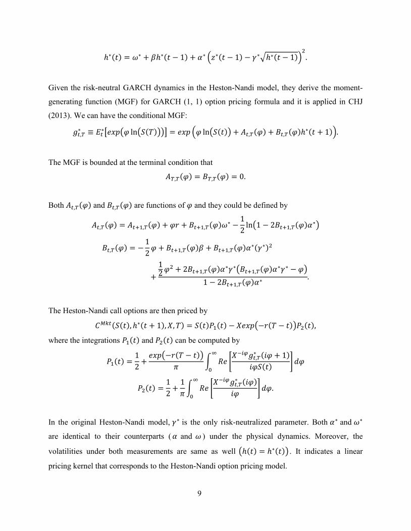
Given the risk-neutral GARCH dynamics in the Heston-Nandi model, they derive the moment-

generating function (MGF) for GARCH (1, 1) option pricing formula and it is applied in CHJ

(2013). We can have the conditional MGF:

𝑔𝑡,𝑇∗ ≡ 𝐸𝑡

∗[𝑒𝑥𝑝(𝜑 ln(𝑆(𝑇)))] = 𝑒𝑥𝑝 (𝜑 ln(𝑆(𝑡)) + 𝐴𝑡,𝑇(𝜑) + 𝐵𝑡,𝑇(𝜑)ℎ∗(𝑡 + 1)).

The MGF is bounded at the terminal condition that

𝐴𝑇,𝑇(𝜑) = 𝐵𝑇,𝑇(𝜑) = 0.

Both 𝐴𝑡,𝑇(𝜑) and 𝐵𝑡,𝑇(𝜑) are functions of 𝜑 and they could be defined by

𝐴𝑡,𝑇(𝜑) = 𝐴𝑡+1,𝑇(𝜑) + 𝜑𝑟 + 𝐵𝑡+1,𝑇(𝜑)𝜔∗ −1

2ln(1 − 2𝐵𝑡+1,𝑇(𝜑)𝛼∗)

𝐵𝑡,𝑇(𝜑) = −1

2𝜑 + 𝐵𝑡+1,𝑇(𝜑)𝛽 + 𝐵𝑡+1,𝑇(𝜑)𝛼∗(𝛾∗)2

+

12 𝜑2 + 2𝐵𝑡+1,𝑇(𝜑)𝛼∗𝛾∗(𝐵𝑡+1,𝑇(𝜑)𝛼∗𝛾∗ − 𝜑)

1 − 2𝐵𝑡+1,𝑇(𝜑)𝛼∗.

The Heston-Nandi call options are then priced by

𝐶𝑀𝑘𝑡(𝑆(𝑡), ℎ∗(𝑡 + 1), 𝑋, 𝑇) = 𝑆(𝑡)𝑃1(𝑡) − 𝑋𝑒𝑥𝑝(−𝑟(𝑇 − 𝑡))𝑃2(𝑡),

where the integrations 𝑃1(𝑡) and 𝑃2(𝑡) can be computed by

𝑃1(𝑡) =1

2+

𝑒𝑥𝑝(−𝑟(𝑇 − 𝑡))

𝜋∫ 𝑅𝑒 [

𝑋−𝑖𝜑𝑔𝑡,𝑇∗ (𝑖𝜑 + 1)

𝑖𝜑𝑆(𝑡)] 𝑑𝜑

∞

0

𝑃2(𝑡) =1

2+

1

𝜋∫ 𝑅𝑒 [

𝑋−𝑖𝜑𝑔𝑡,𝑇∗ (𝑖𝜑)

𝑖𝜑] 𝑑𝜑

∞

0

.

In the original Heston-Nandi model, 𝛾∗ is the only risk-neutralized parameter. Both 𝛼∗ and 𝜔∗

are identical to their counterparts ( 𝛼 and 𝜔 ) under the physical dynamics. Moreover, the

volatilities under both measurements are same as well (ℎ(𝑡) = ℎ∗(𝑡)) . It indicates a linear

pricing kernel that corresponds to the Heston-Nandi option pricing model.

10

2.3 GARCH Pricing Kernel

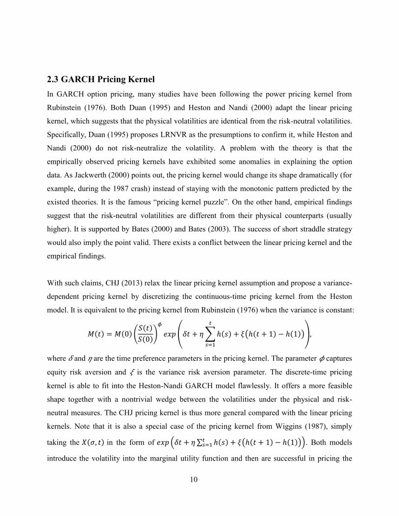
In GARCH option pricing, many studies have been following the power pricing kernel from

Rubinstein (1976). Both Duan (1995) and Heston and Nandi (2000) adapt the linear pricing

kernel, which suggests that the physical volatilities are identical from the risk-neutral volatilities.

Specifically, Duan (1995) proposes LRNVR as the presumptions to confirm it, while Heston and

Nandi (2000) do not risk-neutralize the volatility. A problem with the theory is that the

empirically observed pricing kernels have exhibited some anomalies in explaining the option

data. As Jackwerth (2000) points out, the pricing kernel would change its shape dramatically (for

example, during the 1987 crash) instead of staying with the monotonic pattern predicted by the

existed theories. It is the famous “pricing kernel puzzle”. On the other hand, empirical findings

suggest that the risk-neutral volatilities are different from their physical counterparts (usually

higher). It is supported by Bates (2000) and Bates (2003). The success of short straddle strategy

would also imply the point valid. There exists a conflict between the linear pricing kernel and the

empirical findings.

With such claims, CHJ (2013) relax the linear pricing kernel assumption and propose a variance-

dependent pricing kernel by discretizing the continuous-time pricing kernel from the Heston

model. It is equivalent to the pricing kernel from Rubinstein (1976) when the variance is constant:

𝑀(𝑡) = 𝑀(0) (𝑆(𝑡)

𝑆(0))

𝜙

𝑒𝑥𝑝 (𝛿𝑡 + 𝜂 ∑ ℎ(𝑠)

𝑡

𝑠=1

+ 𝜉(ℎ(𝑡 + 1) − ℎ(1))),

where 𝛿 and 𝜂 are the time preference parameters in the pricing kernel. The parameter 𝜙 captures

equity risk aversion and 𝜉 is the variance risk aversion parameter. The discrete-time pricing

kernel is able to fit into the Heston-Nandi GARCH model flawlessly. It offers a more feasible

shape together with a nontrivial wedge between the volatilities under the physical and risk-

neutral measures. The CHJ pricing kernel is thus more general compared with the linear pricing

kernels. Note that it is also a special case of the pricing kernel from Wiggins (1987), simply

taking the 𝑋(𝜎, 𝑡) in the form of 𝑒𝑥𝑝 (𝛿𝑡 + 𝜂 ∑ ℎ(𝑠)𝑡𝑠=1 + 𝜉(ℎ(𝑡 + 1) − ℎ(1))). Both models

introduce the volatility into the marginal utility function and then are successful in pricing the

11

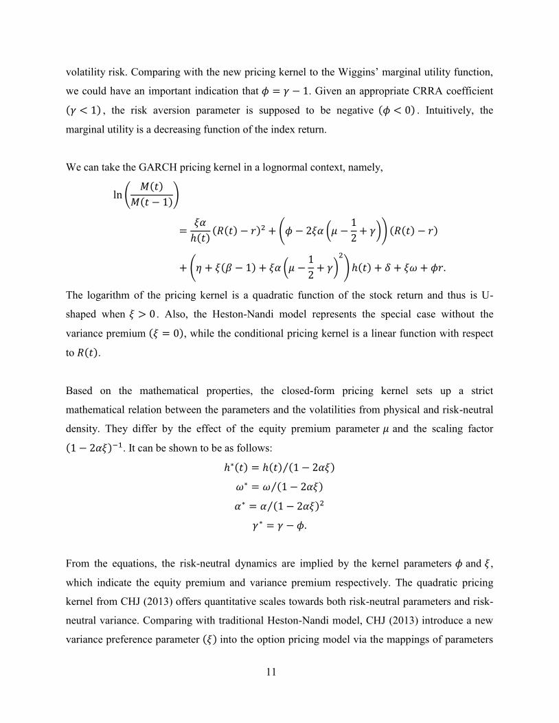
volatility risk. Comparing with the new pricing kernel to the Wiggins’ marginal utility function,

we could have an important indication that 𝜙 = 𝛾 − 1. Given an appropriate CRRA coefficient

(𝛾 < 1) , the risk aversion parameter is supposed to be negative (𝜙 < 0) . Intuitively, the

marginal utility is a decreasing function of the index return.

We can take the GARCH pricing kernel in a lognormal context, namely,

ln (𝑀(𝑡)

𝑀(𝑡 − 1))

=𝜉𝛼

ℎ(𝑡)(𝑅(𝑡) − 𝑟)2 + (𝜙 − 2𝜉𝛼 (𝜇 −

1

2+ 𝛾)) (𝑅(𝑡) − 𝑟)

+ (𝜂 + 𝜉(𝛽 − 1) + 𝜉𝛼 (𝜇 −1

2+ 𝛾)

2

) ℎ(𝑡) + 𝛿 + 𝜉𝜔 + 𝜙𝑟.

The logarithm of the pricing kernel is a quadratic function of the stock return and thus is U-

shaped when 𝜉 > 0 . Also, the Heston-Nandi model represents the special case without the

variance premium (𝜉 = 0), while the conditional pricing kernel is a linear function with respect

to 𝑅(𝑡).

Based on the mathematical properties, the closed-form pricing kernel sets up a strict

mathematical relation between the parameters and the volatilities from physical and risk-neutral

density. They differ by the effect of the equity premium parameter 𝜇 and the scaling factor

(1 − 2𝛼𝜉)−1. It can be shown to be as follows:

ℎ∗(𝑡) = ℎ(𝑡) (1 − 2𝛼𝜉)⁄

𝜔∗ = 𝜔 (1 − 2𝛼𝜉)⁄

𝛼∗ = 𝛼 (1 − 2𝛼𝜉)2⁄

𝛾∗ = 𝛾 − 𝜙.

From the equations, the risk-neutral dynamics are implied by the kernel parameters 𝜙 and 𝜉,

which indicate the equity premium and variance premium respectively. The quadratic pricing

kernel from CHJ (2013) offers quantitative scales towards both risk-neutral parameters and risk-

neutral variance. Comparing with traditional Heston-Nandi model, CHJ (2013) introduce a new

variance preference parameter (𝜉) into the option pricing model via the mappings of parameters

12

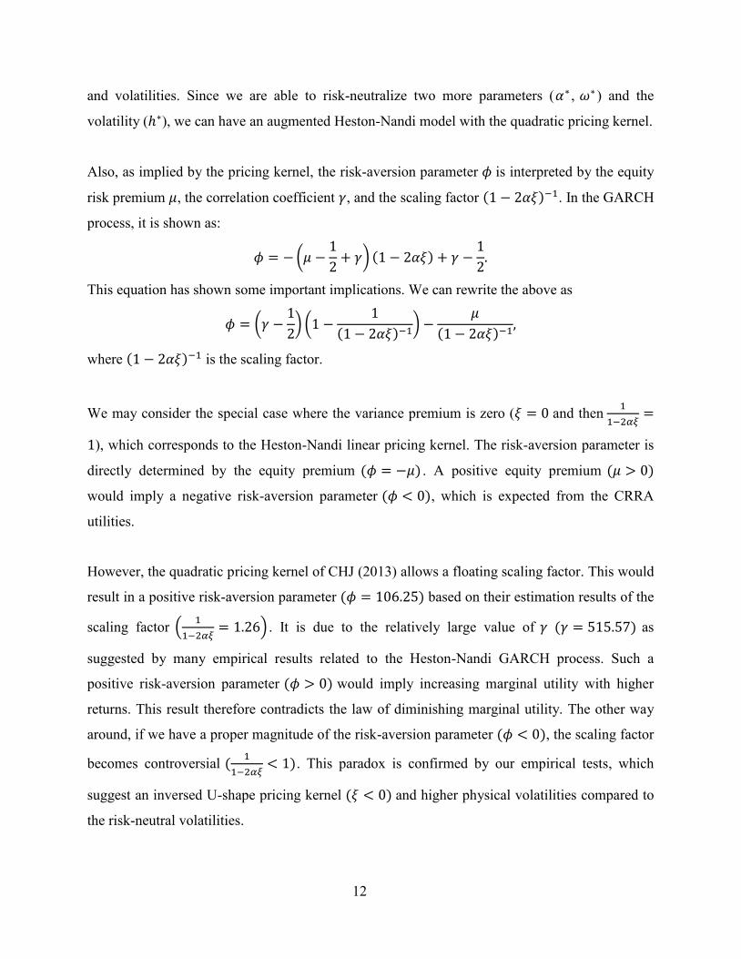
and volatilities. Since we are able to risk-neutralize two more parameters (𝛼∗ , 𝜔∗ ) and the

volatility (ℎ∗), we can have an augmented Heston-Nandi model with the quadratic pricing kernel.

Also, as implied by the pricing kernel, the risk-aversion parameter 𝜙 is interpreted by the equity

risk premium 𝜇, the correlation coefficient 𝛾, and the scaling factor (1 − 2𝛼𝜉)−1. In the GARCH

process, it is shown as:

𝜙 = − (𝜇 −1

2+ 𝛾) (1 − 2𝛼𝜉) + 𝛾 −

1

2.

This equation has shown some important implications. We can rewrite the above as

𝜙 = (𝛾 −1

2) (1 −

1

(1 − 2𝛼𝜉)−1) −

𝜇

(1 − 2𝛼𝜉)−1,

where (1 − 2𝛼𝜉)−1 is the scaling factor.

We may consider the special case where the variance premium is zero (𝜉 = 0 and then 1

1−2𝛼𝜉=

1), which corresponds to the Heston-Nandi linear pricing kernel. The risk-aversion parameter is

directly determined by the equity premium (𝜙 = −𝜇) . A positive equity premium (𝜇 > 0)

would imply a negative risk-aversion parameter (𝜙 < 0), which is expected from the CRRA

utilities.

However, the quadratic pricing kernel of CHJ (2013) allows a floating scaling factor. This would

result in a positive risk-aversion parameter (𝜙 = 106.25) based on their estimation results of the

scaling factor (1

1−2𝛼𝜉= 1.26) . It is due to the relatively large value of 𝛾 (𝛾 = 515.57) as

suggested by many empirical results related to the Heston-Nandi GARCH process. Such a

positive risk-aversion parameter (𝜙 > 0) would imply increasing marginal utility with higher

returns. This result therefore contradicts the law of diminishing marginal utility. The other way

around, if we have a proper magnitude of the risk-aversion parameter (𝜙 < 0), the scaling factor

becomes controversial (1

1−2𝛼𝜉< 1). This paradox is confirmed by our empirical tests, which

suggest an inversed U-shape pricing kernel (𝜉 < 0) and higher physical volatilities compared to

the risk-neutral volatilities.

13

3 Estimation

3.1 Data

The estimations include both index and option data. We use different indices and their

corresponding options from both Canadian and American markets, as represented by S&P TSX

60 (SXO) and Dow Jones Industrial Average (DJX).

The index sample period extends from Jan. 1, 2005 to Dec. 31, 2013 for SXO and Jan. 1, 1990 to

Dec. 31, 2010 for DJX. In order to have more weight on the optimization, such long-ranged data

would guarantee enough information from the index returns. Empirically, the balance between

the two parts of the estimation is very important, considering the sensitivity of the parameters

when performing the optimization. Also, the long-track of the index data is able to stabilize the

equity premium.

Regarding to the option data, we collect the out-of-the-money (OTM) put and call options of

S&P TSX 60 (SXO) from Jan. 1, 2009 to Dec. 31, 2013 and those of Dow Jones Industrial

Average (DJX) from Oct. 1, 1997 to Dec. 31, 2010. All the option data are obtained from the

Montreal Exchange and the Option Metrics. The option value is defined as the midpoint of the

bid and ask prices. The moneyness is computed by the implied futures price 𝐹 divided by the

strike price 𝑋. We pick both SXO and DJX options with maturity between 14 days and 180 days.

We eliminate all the options whose quotes are lower than $3/8, considering the impact of the

price discreteness. The risk-free rate is fixed at 5 percent.

In both samples, we only use the Wednesday options for our empirical estimations. It would

allow us to study a long time series of the options. Also, Wednesday is least likely to be a

holiday, while Monday and Friday are affected by the weekday effect. Early literatures (Dumas,

Fleming, and Whaley, 1998; Heston and Nandi, 2000) have largely used the option data for

Wednesdays. We pick 6 options with the highest volume from each available maturity when

estimating with the Dow Jones options. For the Canadian options, we keep all the available

options from each maturity. It is mainly because the inactivity of the SXO options would cause

an imbalance of likelihoods during the estimation.

14

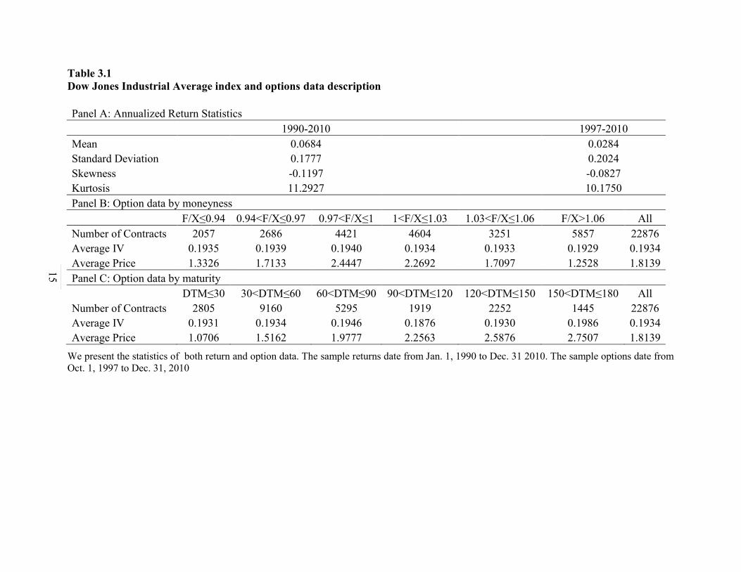
Table 3.1 provides both the returns and options data description for the Dow Jones Industrial

Average index. We present the return statistics that cover the time periods from both the return

sample and option sample. The standard deviation of sample returns is close to the average

option-implied volatility. With regards to the higher moments of the return distribution, the table

shows a slight negative skewness and significant excess kurtosis. We also present descriptive

statistics for the option data. The implied volatility is relatively stable across the sample

moneyness and maturity range. It is notably different from the S&P 500 index (SPX) options

since they have higher implied volatility from OTM put options. More important, the SPX

options with longer maturity have significantly larger implied volatilities. The different implied

volatility patterns from the indices initially provide empirical supports to our overreaction tests

in the next section.

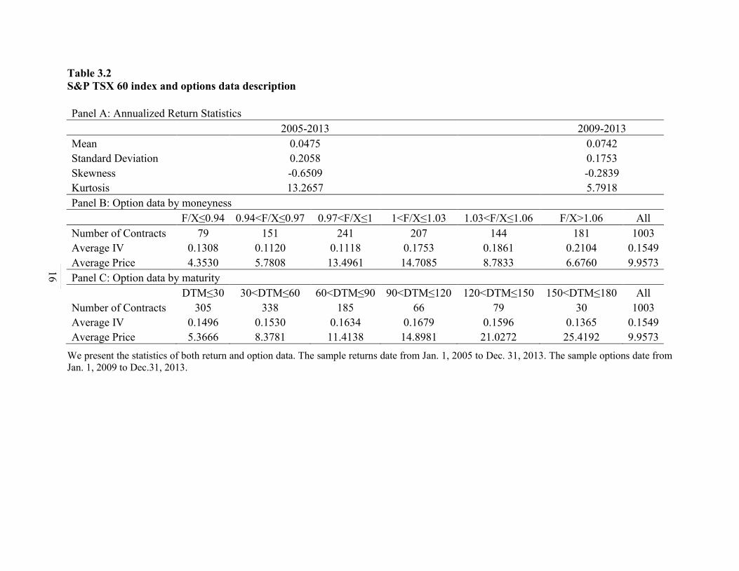
Table 3.2 presents the statistics of the S&P TSX 60 sample data. Compared to the Dow Jones

Industrial Average sample, the S&P TSX 60 index and options behave quite differently. First,

the standard deviation of returns is higher than the average option-implied volatility. We also

observe stronger negative skewness from the returns. For the option data, the OTM put options

have the largest implied volatility, which is consistent with the SPX options. Given the

differentiations between the two samples, it is important for us to test the new pricing kernel’s

ability to fit both data.

15

Table 3.1

Dow Jones Industrial Average index and options data description

Panel A: Annualized Return Statistics

1990-2010 1997-2010

Mean

0.0684

0.0284

Standard Deviation

0.1777

0.2024

Skewness

-0.1197

-0.0827

Kurtosis 11.2927 10.1750

Panel B: Option data by moneyness

F/X≤0.94 0.94<F/X≤0.97 0.97<F/X≤1 1<F/X≤1.03 1.03<F/X≤1.06 F/X>1.06 All

Number of Contracts 2057 2686 4421 4604 3251 5857 22876

Average IV 0.1935 0.1939 0.1940 0.1934 0.1933 0.1929 0.1934

Average Price 1.3326 1.7133 2.4447 2.2692 1.7097 1.2528 1.8139

Panel C: Option data by maturity

DTM≤30 30<DTM≤60 60<DTM≤90 90<DTM≤120 120<DTM≤150 150<DTM≤180 All


Average IV 0.1931 0.1934 0.1946 0.1876 0.1930 0.1986 0.1934

Average Price 1.0706 1.5162 1.9777 2.2563 2.5876 2.7507 1.8139

We present the statistics of both return and option data. The sample returns date from Jan. 1, 1990 to Dec. 31 2010. The sample options date from

Oct. 1, 1997 to Dec. 31, 2010

16

Table 3.2

S&P TSX 60 index and options data description

Panel A: Annualized Return Statistics

2005-2013 2009-2013

Mean

0.0475

0.0742

Standard Deviation

0.2058

0.1753

Skewness

-0.6509

-0.2839

Kurtosis 13.2657 5.7918

Panel B: Option data by moneyness

F/X≤0.94 0.94<F/X≤0.97 0.97<F/X≤1 1<F/X≤1.03 1.03<F/X≤1.06 F/X>1.06 All


Average IV 0.1308 0.1120 0.1118 0.1753 0.1861 0.2104 0.1549

Average Price 4.3530 5.7808 13.4961 14.7085 8.7833 6.6760 9.9573

Panel C: Option data by maturity

DTM≤30 30<DTM≤60 60<DTM≤90 90<DTM≤120 120<DTM≤150 150<DTM≤180 All


Average IV 0.1496 0.1530 0.1634 0.1679 0.1596 0.1365 0.1549

Average Price 5.3666 8.3781 11.4138 14.8981 21.0272 25.4192 9.9573

We present the statistics of both return and option data. The sample returns date from Jan. 1, 2005 to Dec. 31, 2013. The sample options date from

Jan. 1, 2009 to Dec.31, 2013.

17

3.2 Joint Likelihood Estimation

The maximum likelihood estimation is first developed by Duan (1995) for derivatives pricing.

He uses the prices of derivative contracts to calculate the likelihoods obtained from an

unobservable return process. The parameters are thus obtained from the maximization of

likelihoods. Empirical performance of the method is consistent with the results from Merton

(1977) theoretical model that equity volatility is stochastic. Following this methodology, the

maximum likelihood estimation has been widely applied within the domain of option pricing

both theoretically and empirically.

In our study the estimation of the quadratic pricing kernel is based on a joint likelihood

maximization containing both the index returns and the option prices. Since the conditional

density of the daily return is normal distributed, we have the following return log likelihood:

ln 𝐿𝑅 ∝ −1

2∑ {ln(ℎ(𝑡)) + (𝑅(𝑡) − 𝑟 − 𝜇ℎ(𝑡))

2ℎ(𝑡)⁄ }

𝑇

𝑡=1

.

With regards to the likelihood from options, CHJ (2013) define a volatility-weighted error based

on the Black-Scholes Vega (BSV):

휀𝑖 = (𝐶𝑖𝑀𝑘𝑡 − 𝐶𝑖

𝑀𝑜𝑑) 𝐵𝑆𝑉𝑖𝑀𝑘𝑡⁄ ,

where 𝐶𝑖𝑀𝑘𝑡 and 𝐶𝑖

𝑀𝑜𝑑 are market and model prices of the 𝑖𝑡ℎ option, respectively. The model

price is computed from the augmented Heston-Nandi model with new parameters from the

pricing kernel. They further define the option log likelihood with respects to the BSV:

ln 𝐿𝑜 ∝ −1

2∑{ln(𝑠𝜀

2) + 휀𝑖2 𝑠𝜀

2⁄ }

𝑇

𝑡=1

,

where �̂�𝜀2 =

1

𝑁∑ 휀𝑖

2𝑁𝑖=1 for sample estimating.

In order to estimate the pricing kernels, which connect the information from index and options,

we optimize a joint likelihood

max𝛩,𝛩∗

ln 𝐿𝑅 + ln 𝐿𝑜 ,

where 𝛩 = {𝜔, 𝛼, 𝛽, 𝛾, 𝜇} and 𝛩∗ = {𝜔∗, 𝛼∗, 𝛾∗}. All the risk-neutral parameters are linked with

the physical parameters by the mappings.

18

We estimate three types of pricing kernels. The first one comes with no risk premium. It refers to

the setting 𝜇 = 𝜉 = 0. It is the most fundamental case that refers to the logarithm of the pricing

kernel is a constant with respect to the return. The second one is identical to the Heston-Nandi

(2000) linear pricing kernel, which contains the equity risk only, as specified by 𝜇 ≠ 0 and 𝜉 = 0.

The last case amounts to the quadratic pricing kernel developed by CHJ (2013). Given two

preference parameters (𝜙 and 𝜉) in the transformation, the estimation would result in non-zero 𝜇

and 𝜉 . The first two pricing kernels can be considered as the special cases of the quadratic

pricing kernel. All of them would be estimated by the joint-likelihood maximizations.

19

Table 3.3

Joint maximum likelihood estimation with Dow Jones Industrial Average index and

options

Physical

Parameters No Premia Equity Premium Only

Equity and Volatility

Premia

ω 0 0 0

α 7.24E-07 7.25E-07 1.23E-06

β 0.7029 0.7030 0.6724

γ 630.1274 628.7239 508.1599

μ 0 1.1824 1.1824

Risk-neutral

Parameters

1/(1-2αξ) 1 1 0.7457

ω* 0 0 0

α* 7.24E-07 7.25E-07 6.83E-07

β* 0.7029 0.7030 0.6724

γ* 630.1274 629.9063 682.8595

Pricing Kernel

Parameters

ϕ 0 -1.1824 -174.6996

ξ 0 0 -1.39E+05

Total Likelihood 52182.2917 52182.4141 52296.8818

From Returns 17042.0208 17042.2308 17126.7787

From Options 35140.2709 35140.1833 35170.1030

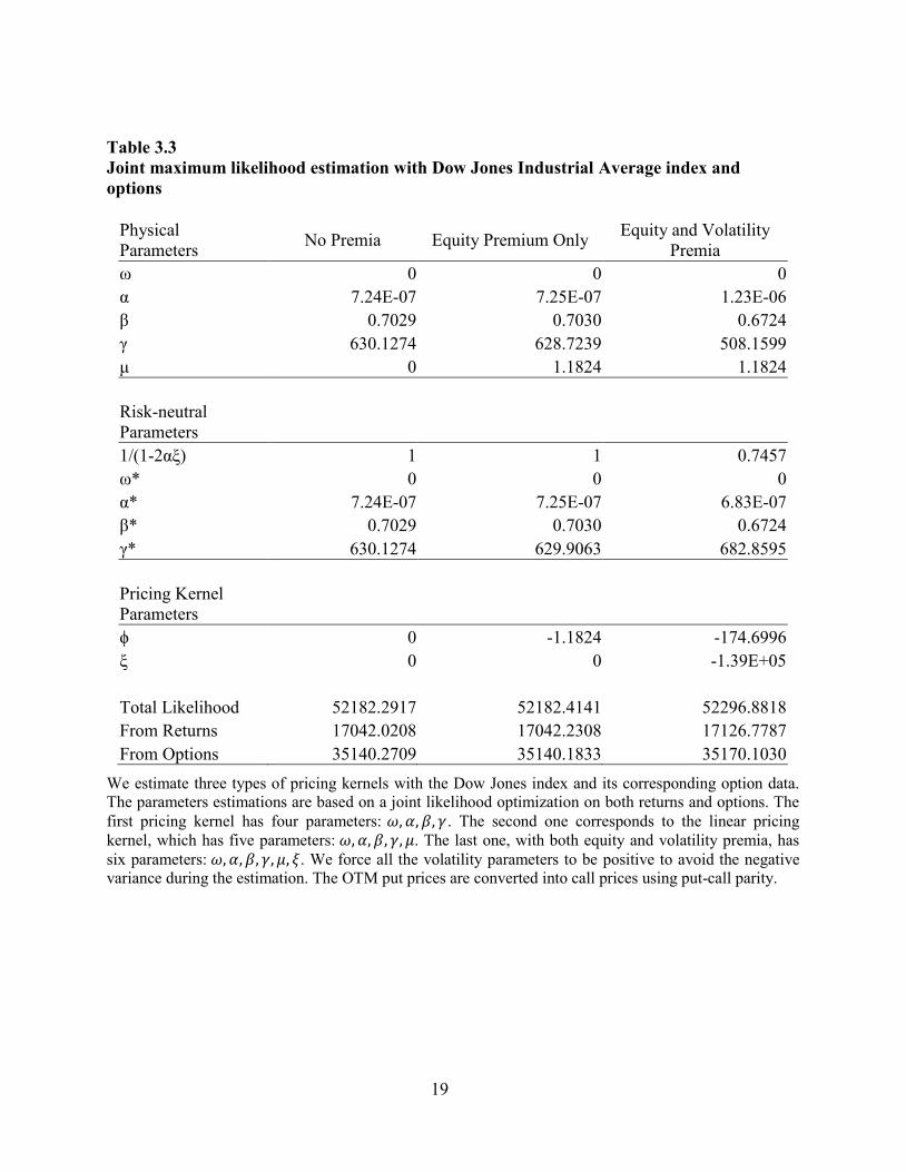
We estimate three types of pricing kernels with the Dow Jones index and its corresponding option data.

The parameters estimations are based on a joint likelihood optimization on both returns and options. The

first pricing kernel has four parameters: 𝜔, 𝛼, 𝛽, 𝛾. The second one corresponds to the linear pricing

kernel, which has five parameters: 𝜔, 𝛼, 𝛽, 𝛾, 𝜇. The last one, with both equity and volatility premia, has

six parameters: 𝜔, 𝛼, 𝛽, 𝛾, 𝜇, 𝜉. We force all the volatility parameters to be positive to avoid the negative

variance during the estimation. The OTM put prices are converted into call prices using put-call parity.

20

Table 3.4

Joint maximum likelihood estimation with S&P TSX 60 index and options

Physical



Premia

ω 0 0 0

α 9.29E-07 9.29E-07 1.44E-06

β 0.8701 0.8704 0.7943

γ 354.1281 352.1645 366.7981

μ 0 1.4918 1.4918

Risk-neutral

Parameters

1/(1-2αξ) 1 1 0.6368

ω* 0 0 0

α* 9.29E-07 9.29E-07 5.82E-07

β* 0.8701 0.8704 0.7943

γ* 354.1281 353.6563 578.0323

Pricing Kernel

Parameters

ϕ 0 -1.4918 -211.2342

ξ 0 0 -1.99E+05


From Returns 7127.7375 7128.0082 7180.0521

From Options 2110.8759 2110.7257 2142.5690

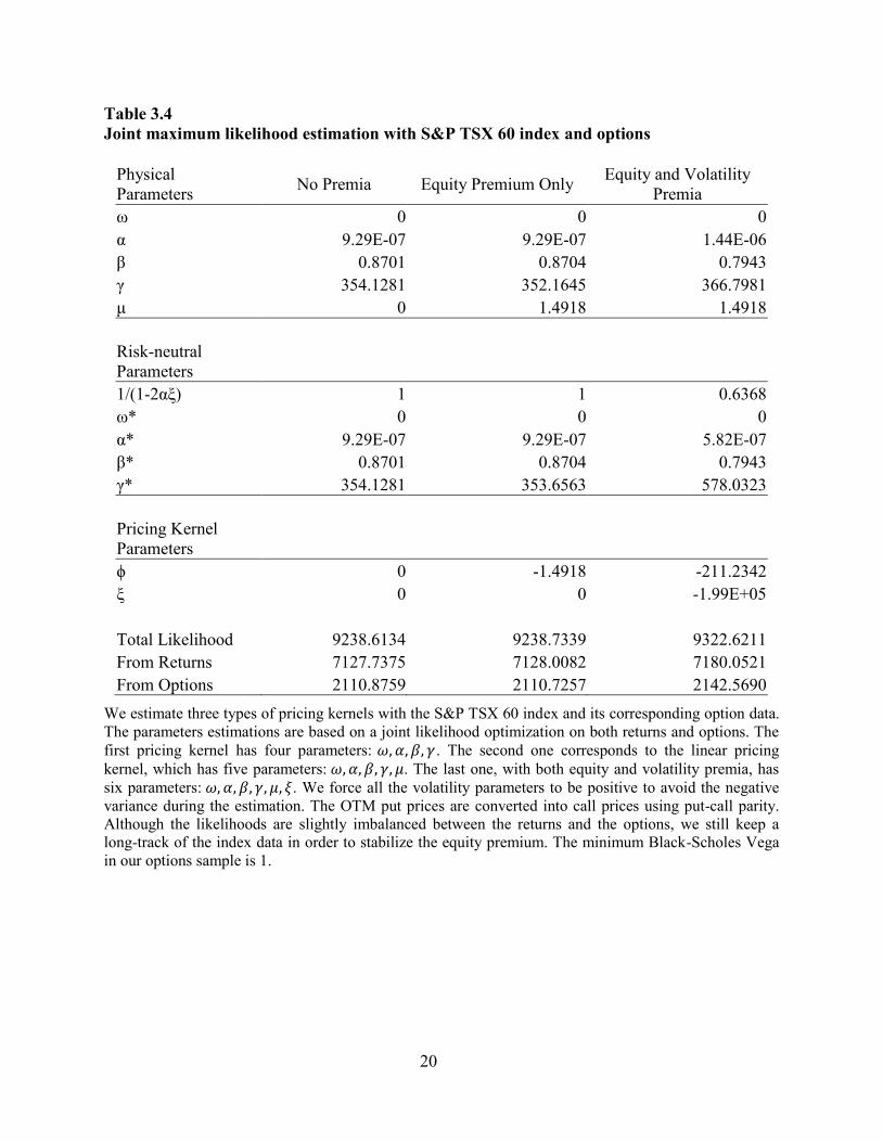
We estimate three types of pricing kernels with the S&P TSX 60 index and its corresponding option data.






Although the likelihoods are slightly imbalanced between the returns and the options, we still keep a

long-track of the index data in order to stabilize the equity premium. The minimum Black-Scholes Vega

in our options sample is 1.

21

Table 3.5

Joint maximum likelihood estimation with S&P 500 index and options

Physical



Premia

ω 0 0 0

α 1.410E-06 1.410E-06 8.887E-07

β 0.755 0.755 0.756

γ 411.19 409.63 515.57

μ 0 1.594 1.594

Risk-neutral

Parameters

1/(1-2αξ) 1 1 1.2638

ω* 0 0 0

α* 1.410E-06 1.410E-06 1.419E-06

β* 0.755 0.755 0.756

γ* 411.19 411.23 409.32

Pricing Kernel

Parameters

ϕ 0 -1.594 106.25

ξ 0 0 1.17E+05


From Returns 17673.7 17681.0 17749.2

From Options 38729.7 38729.8 38731.6

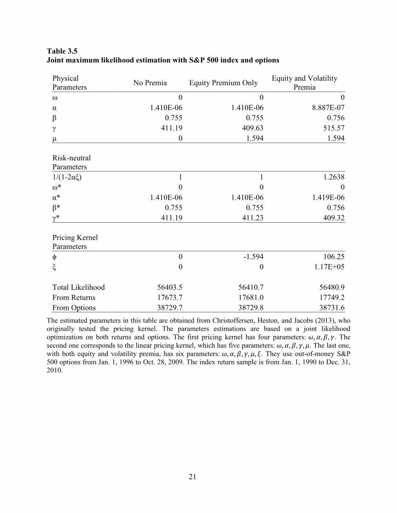
The estimated parameters in this table are obtained from Christoffersen, Heston, and Jacobs (2013), who

originally tested the pricing kernel. The parameters estimations are based on a joint likelihood

optimization on both returns and options. The first pricing kernel has four parameters: 𝜔, 𝛼, 𝛽, 𝛾. The

second one corresponds to the linear pricing kernel, which has five parameters: 𝜔, 𝛼, 𝛽, 𝛾, 𝜇. The last one,

with both equity and volatility premia, has six parameters: 𝜔, 𝛼, 𝛽, 𝛾, 𝜇, 𝜉. They use out-of-money S&P

500 options from Jan. 1, 1996 to Oct. 28, 2009. The index return sample is from Jan. 1, 1990 to Dec. 31,

2010.

22

Table 3.3 and Table 3.4 present the results for the joint likelihood estimation of the parameters,

using different indices and options data (SXO and DJX respectively). The first column shows the

estimation results without premia. Column 2 amounts to the linear pricing kernel, which

corresponds to the Heston-Nandi model. The last column represents the CHJ case that allows

both equity and variance premium. It stands for the quadratic pricing kernel with an independent

variance premium. Despite the differences between two samples from the descriptive statistics,

both tables show that the total likelihoods are very close from the first two cases. Based on the

likelihood ratio test, which compares the difference between the log-likelihood values following

the chi-square test, insignificant statistics are implied by the estimation results. The linear pricing

kernel is not able to provide strong improvements to the model’s empirical performance

according to the test. It is mainly because we use the constant equity premium during the

estimation in order to ensure its proper calibration. The two cases are thus not statistically

differentiated.

Consider the quadratic pricing kernel in Column 3. When adding the independent volatility

premium (𝜉) to the linear pricing kernel specified in Column 2, the total likelihood function

improves dramatically (from 52182.4 to 52296.9 in Table 3.3 and from 9238.7 to 9322.6 in

Table 3.4). As a result, the likelihood ratio test statistics (228.9354 from Table 3.3 and 167.7744

from Table 3.4) are both significant at the 0.1% level. The quadratic pricing kernel has a great

improvement in terms of the model performance from this perspective. However, both results

from DJX and SXO data demonstrate that the scaling factor is less than 1. It would result in a

negative 𝜉 due to the positive α and thus an inverted U-shaped pricing kernel. On the other hand,

since the risk-neutral volatility is widely accepted to be higher than the physical volatility, a

negative volatility premium implied by 𝜉 is also against the empirical findings. We are confident

to conclude that the new pricing kernel fails to fit the data from both American and Canadian

market.

Meanwhile, as Table 3.5 presents, the original CHJ estimation has also shown the contradiction.

Although the scaling factor (1 − 2𝛼𝜉)−1 is correctly estimated by CHJ (2013) with a positive

variance preference (𝜉 = 1.17E + 05), the risk-aversion parameter is misfit from the newly

developed GARCH pricing kernel (𝜙 = 106.25). Such a large positive risk-aversion parameter

23

is inconsistent with the CRRA-type utility, which generates decreasing marginal utility with

higher returns, accordingly leaving a bias against the law of diminishing marginal utility.

In summary, the empirical results are consistent with our previous analysis. The new GARCH

model with quadratic pricing kernel does not fit the indices and options data properly. The

magnitude problem raised by the quadratic pricing kernel for the GARCH model tends to be

unsolvable. A more reasonable explanation is the strict quantitative relations located by the

parameters and the volatilities. For instance, as a single representative, the pricing kernel

presented by the corresponding market behavior is irreconcilable. It is also pointed by Jackwerth

(2000). In recent work, Barone-Adesi, Mancini. and Shefrin (2013) have provided strong

empirical supports to this viewpoint. They develop a model that nests investors’ sentiment from

the option and stock prices and estimate the empirical pricing kernels with a weekly rolling

window. The pricing kernel is U-shaped by 2003 and inverted-U by 2005. The results show that

investors tend to be overconfident when market is growing with low volatility. They can be also

underconfident during crisis periods. The observed overconfidence is a main driving force of the

pricing kernel puzzle. From this perspective, the closed-form U-shape pricing kernel is not a

good representative of the investors.

24

4 The Overreaction Test

In our study the pricing kernels are estimated through a joint-likelihood function. Since the

likelihoods from option data are based on the Vega-weighted pricing errors, it is important to test

the model’s ability to observe the volatility patterns. An indirect but efficient way is to test the

consistency between the actual option prices and GARCH model option prices in predicting the

long-term implied volatility overreaction.

The overreaction phenomenon in the options market is initially tested by Stein (1989) with the

S&P 100 index options. The study starts with the term structure of implied volatility. We assume

an instantaneous volatility 𝜎𝑡, which follows a continuous time mean-reverting AR1 process:

𝑑𝜎𝑡 = −𝛼(𝜎𝑡 − 𝜎) 𝑑𝑡 + 𝛽𝜎𝑡𝑑𝑧.

The expectation of volatility at time 𝑡 + 𝑗 is given by

𝐸𝑡(𝜎𝑡+𝑗) = 𝜎 + 𝜌𝑗(𝜎𝑡 − 𝜎),

where 𝜌 = 𝑒𝑥𝑝(−𝛼) is and 𝑗 is measured by the number of weeks. Given an option at time 𝑡

with 𝑇 remaining until expiration, the implied volatility of it equals to the average expected

instantaneous volatility:

𝐼𝑉𝑡(𝑡) =1

𝑇∫ [𝜎 + 𝜌𝑗(𝜎𝑡 − 𝜎)]

𝑇

𝑗=0

𝑑𝑗 = 𝜎 +𝜌𝑇 − 1

𝑇 ln 𝜌[𝜎𝑡 − 𝜎].

Since the instantaneous volatility is unobservable, we can take both a short-term (ST) option and

a long-term (LT) option in order to test the term structure without the instantaneous volatility:

(𝐼𝑉𝑡𝐿𝑇 − 𝜎) =

𝑆𝑇(𝜌𝐿𝑇 − 1)

𝐿𝑇(𝜌𝑆𝑇 − 1)(𝐼𝑉𝑡

𝑆𝑇 − 𝜎).

This equation can be exactly approximated when the gap between short-term and long-term is

one month (𝑗 = 4):

(𝐼𝑉𝑡𝐿𝑇 − 𝜎) ≈

(1 + 𝜌4)

2(𝐼𝑉𝑡

𝑆𝑇 − 𝜎).

Again, we reintroduce the expectation 𝐸𝑡(𝜎𝑡+𝑗) = 𝜎 + 𝜌𝑗(𝜎𝑡 − 𝜎), the above approximation can

be rewritten in a more general form as

25

(𝐼𝑉𝑡𝐿𝑇 − 𝜎) =

1

2(𝐼𝑉𝑡

𝑆𝑇 − 𝜎) +1

2𝐸𝑡(𝐼𝑉𝑡+4

𝑆𝑇 − 𝜎),

which is equivalent to

𝐸[(𝐼𝑉𝑡+4𝑆𝑇 − 𝐼𝑉𝑡

𝑆𝑇) − 2(𝐼𝑉𝑡𝐿𝑇 − 𝐼𝑉𝑡

𝑆𝑇)] = 0.

We can simply take that the expected change in implied volatility is twice the slope of the term

structure of the implied volatility. The volatility reaction study tests whether the “term structure”

of implied volatility is consistent with rational expectations. Intuitively, future implied

volatilities are systematically lower than predictions made by the term structure of volatility. The

other way around, long-term options tend to overreact to changes in short-term volatility. It

would be more significant when the term structure of implied volatility is steep. Given the

expectation, Stein (1989) estimates the following OLS regression to test the overreaction:

(𝐼𝑉𝑡+41𝑀 − 𝐼𝑉𝑡

1𝑀) − 2(𝐼𝑉𝑡2𝑀 − 𝐼𝑉𝑡

1𝑀) = 𝑎0 + 𝑎1𝐼𝑉𝑡1𝑀 + 𝑒𝑡+4.

The parameter 𝑎1 is expected to be negative, indicating that the future implied volatility is

expected to be smaller than the forward forecasts implied by the term structure of volatility. The

regression is performed with at-the-money option data. 1-month maturity is set as short-term and

a 2-month maturity is set as long-term. For a given day, we fit a polynomial for the implied

volatility as a function of the moneyness and maturity. Since the S&P TSX 60 option sample is

not able to provide enough eligible options in order to fit the polynomials, we only run the

regressions from the Dow Jones Industrial Average options.

26

Table 4.1

Long-term volatility overreaction tests

Model Prices

Panel A: Market Prices

Panel B: Equity Premium Only

Panel C: Equity and Volatility

Premia

Sample Coefficient Std. Error t-Statistic Coefficient Std. Error t-Statistic Coefficient Std. Error t-Statistic

1998 -0.2200 0.1487 -1.4793

-0.1631 0.1154 -1.4128

-0.1535 0.1156 -1.3271

1999 -0.1650 0.1128 -1.4627

-0.3020 0.1578 -1.9138

-0.2750 0.1574 -1.7472

2000 -0.3012 0.1487 -2.0258

-1.0843 0.1402 -7.7360

-1.0773 0.1406 -7.6595

2001 -0.2484 0.1282 -1.9372

-0.4795 0.1296 -3.6999

-0.4747 0.1298 -3.6557

2002 -0.2066 0.1187 -1.7414

-0.1094 0.1195 -0.9154

-0.1037 0.1194 -0.8688

2003 0.0860 0.0675 1.2739

0.0592 0.0847 0.6984

0.0813 0.0834 0.9754

2004 -0.7410 0.1406 -5.2689

-0.5311 0.1291 -4.1129

-0.5121 0.1292 -3.9639

2005 -0.6311 0.1349 -4.6776

-0.4995 0.1144 -4.3659

-0.4775 0.1138 -4.1971

2006 0.0896 0.1439 0.6226

0.0808 0.0939 0.8605

0.1045 0.0939 1.1130

2007 -0.1712 0.0841 -2.0368

0.0125 0.1101 0.1135

0.0351 0.1103 0.3183

2008 -0.0176 0.0974 -0.1807

-0.0467 0.0768 -0.6079

-0.0483 0.0768 -0.6287

2009 -0.0961 0.0496 -1.9386

0.0661 0.0393 1.6807

0.0752 0.0390 1.9267

2010 -0.7267 0.1659 -4.3807 -0.3941 0.1222 -3.2245 -0.3716 0.1219 -3.0477

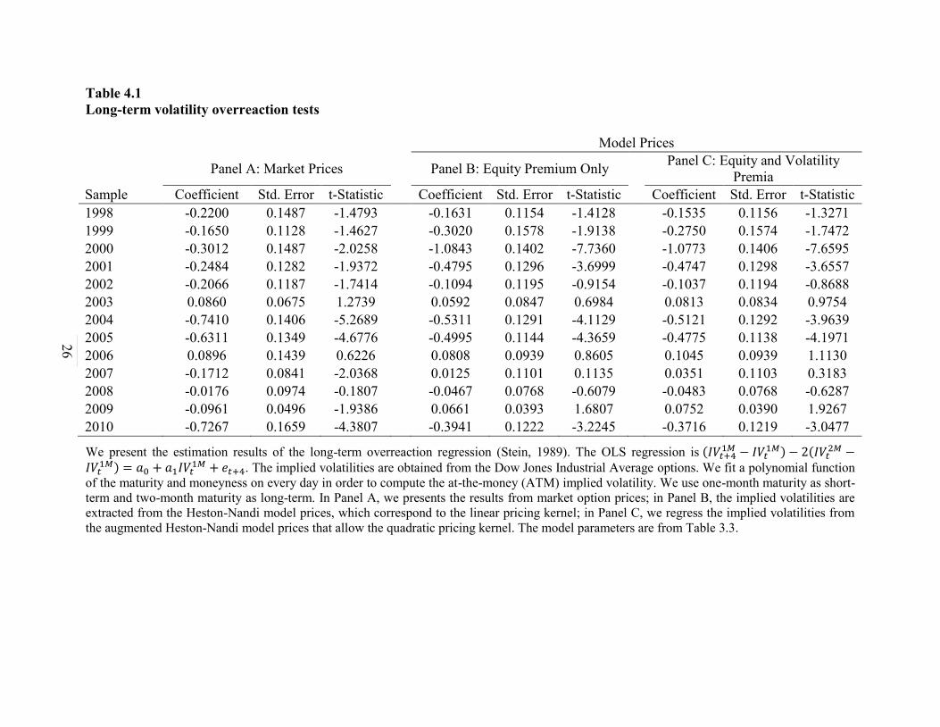
We present the estimation results of the long-term overreaction regression (Stein, 1989). The OLS regression is (𝐼𝑉𝑡+41𝑀 − 𝐼𝑉𝑡

1𝑀) − 2(𝐼𝑉𝑡2𝑀 −

𝐼𝑉𝑡1𝑀) = 𝑎0 + 𝑎1𝐼𝑉𝑡

1𝑀 + 𝑒𝑡+4. The implied volatilities are obtained from the Dow Jones Industrial Average options. We fit a polynomial function

of the maturity and moneyness on every day in order to compute the at-the-money (ATM) implied volatility. We use one-month maturity as short-

term and two-month maturity as long-term. In Panel A, we presents the results from market option prices; in Panel B, the implied volatilities are

extracted from the Heston-Nandi model prices, which correspond to the linear pricing kernel; in Panel C, we regress the implied volatilities from

the augmented Heston-Nandi model prices that allow the quadratic pricing kernel. The model parameters are from Table 3.3.

27

Table 4.1 presents the results from the overreaction tests based on the market, Heston-Nandi

model, and CHJ model option prices. Within most of our sample range, the overreaction

phenomenon is observable. As Table 3.1 shows, the DJX implied volatility is relatively stable

across different maturities. The regression results are thus expected to be insignificant from most

of the sample years. The two exceptional years are 2003 and 2006; the behavior of long-term

implied volatilities indicates slight underreactions. In those years, the regression results still

present consistency between the market and model prices.

However, we also observe inconsistency between the test results in 2007 and 2009. Both the

Heston-Nandi model and the augmented Heston-Nandi model from CHJ (2013) are not able to

present overreactions from the market option prices. It is potentially due to the financial crisis,

while the GARCH dynamics are incapable of modeling the econometrical form of the volatility.

Overall, we can observe the overreaction phenomenon from the DJX options, though it is not as

significant as CHJ (2013) document. Our results are closer to the original empirical tests from

Stein (1989), which presents a relative low t-statistic across each sample year. The regression

parameters are consistent between the market option prices and model option prices, except for

the 2 years during the financial crisis. More important, the two GARCH models that nest the

linear and quadratic pricing kernel respectively are not significantly differentiated from the

overreaction tests.

28

5 Stochastic Dominance Bounds

5.1 Introduction

Since the Black-Scholes model is based on a perfect complete market, it establishes a self-

financing dynamic trading between the stock and risk-free accounts. When there are transaction

costs and the investors cannot continuously hedge their portfolios, the assumption of

completeness would go down.

Most option pricing models have to face constrains from transaction costs given the non-

arbitrage arguments. From this aspect, the stochastic dominance provides an alternative

explanation of option pricing and option trading. Due to the presence of transaction costs, the

market is discrete and the investors are able to trade both the underlying assets and the options.

The stochastic dominance bounds are determined based on the utility maximization principle.

We can identify the mispriced options those provide opportunities to adopt the stochastically

dominating strategies since such violations of upper and lower bounds would bring superior

returns. A feasible feature of the methodology is that the bounds can be derived from any

arbitrary distribution of the stock price. They are free from any presumptions about the utility

function, as in arbitrage.

As motivated by Jackwerth (2000), we apply the stochastic dominance bounds in order to filter

out the mispriced options from the estimation data sample. According to Constantinides and

Perrakis (2002), in a single-period economy, the upper bound with transaction costs for a

European option at any time 𝑡 prior to its expiration is presented as follows:

𝐶̅ = {(1 + 𝑘1) (1 − 𝑘2)⁄ } 𝐸[(𝑆𝑇 − 𝐾)+|𝑆𝑡] 𝑅𝑆𝑇−𝑡⁄

�̅� = 𝐶̅ − (1 − 𝑘2)𝑆(𝑡) (1 + 𝑘1)⁄ + 𝐾 𝑅𝑇−𝑡⁄ ,

where 𝑘 is the transaction cost ratio and 𝑅𝑆 is the expected return on the stock per period.

5.2 Estimation

In order to estimate the distribution of asset returns, we widely follow the methodology from

Constantinides, Jackwerth, and Perrakis (2009), which impose non-parametric forms on both

29

unconditional and conditional distribution of the index returns. The unconditional distribution is

extracted from historical returns as the smoothed histograms using the kernel estimator. They

also estimate conditional densities from a generalized GARCH (1, 1) process and the Black-

Scholes implied volatility (IV).

In our empirical work we use the at-the-money (ATM) S&P 500 call options with moneyness

from 1 to 1.03. Only upper bound violations are tested since most of the violations are those

from the upper bounds (Constantinides, Jackwerth, and Perrakis, 2009). We estimate the

unconditional distribution of the index returns through the kernel estimator. The distribution is

obtained from post-crash monthly index returns between Jan. 1, 1988 and Dec. 31, 2010. The

post-crash data would provide relatively stable distribution and also the pricing kernel. The

monthly return is calculated by 30 calendar day (21 trading day) returns given the historical daily

prices of the S&P 500 index. We define 512 mesh points from the range of the returns. The

cumulative densities are calculated by the integrals. We have some numerical problems with the

extreme probabilities for the beginning and ending states. Following Constantinides, Jackwerth,

and Perrakis (2009), we eliminate such probabilities and rescale the remaining.

The mean expected return is fixed to a 4% premium over the risk-free rate. Empirically we keep

the 5% risk-free rate instead of the floating government bond rates, it is mainly because the

prices of 1-month call options are insensitive to the expected return of the index. We assume the

proportional transaction costs in a single-period economy and the cost ratio is 0.03.

From the data described above, we could generate a kernel density of the distribution. It is

formulated as

𝑓(𝑥) =1

𝑛ℎ∑ 𝐾 (

𝑥 − 𝑋𝑖

ℎ)

𝑛

𝑖=1

,

where 𝑋𝑖 denotes the 𝑖𝑡ℎ state, 𝐾 is the Gaussian density function, and ℎ is the window width, or

the smoothing parameter. Given the properties of the kernel estimator, the window width ℎ is a

key factor when generating the kernel density. For the Gaussian 𝐾(𝑡), the optimal window width

is

30

ℎ𝑜𝑝𝑡 = (4

3)

1 5⁄

𝜎𝑛−1 5⁄ = 1.06𝜎𝑛−1 5⁄ ,

by minimizing the approximate mean integrated square error.

For the S&P 500 index option sample, we have 3533 1-month OTM call options from 1996 to

2010. It is easy to calculate the upper bound of each option from our data sample. 496 of them

violate the stochastic dominance bounds. The violation rate is 14.04%. It is a relatively high ratio

given the fact that we have only filtered all the ATM options. The pricing kernels are tested with

the filtered option data, while the return sample dates from Jan. 1, 1990 to Dec. 31, 2010.

31

Table 5.1

Joint maximum likelihood estimation with S&P 500 index and 1-month call options

Physical



Premia

ω 0 0 0

α 1.22E-06 1.22E-06 2.02E-06

β 0.6949 0.6948 0.6650

γ 485.8554 484.0931 397.4966

μ 0 1.7087 1.7087

Risk-neutral

Parameters

1/(1-2αξ) 1 1 0.6763

ω* 0 0 0

α* 1.22E-06 1.22E-06 9.22E-07

β* 0.6949 0.6948 0.6650

γ* 485.8554 485.8018 590.0827

Pricing Kernel

Parameters

ϕ 0 -1.7087 -192.5861

ξ 0 0 -1.19E+05


From Returns 16956.0588 16957.2425 17073.4207

From Options 9154.0790 9153.7224 9215.5430

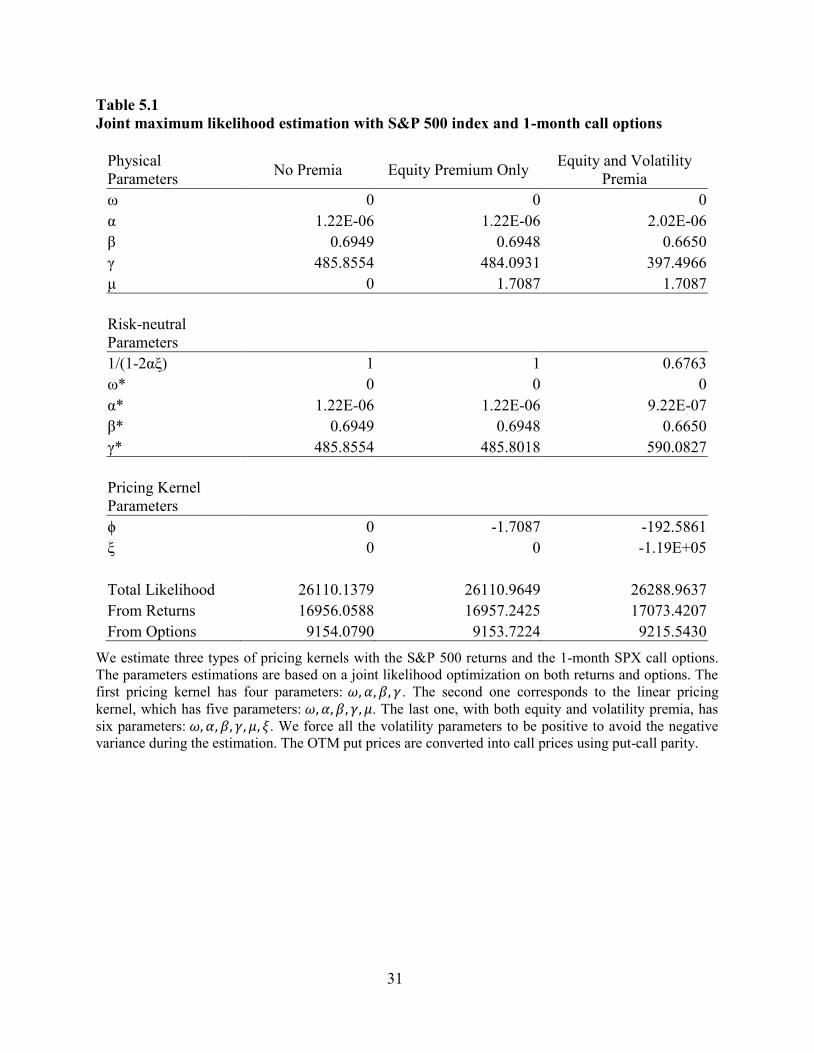
We estimate three types of pricing kernels with the S&P 500 returns and the 1-month SPX call options.






32

Table 5.2

Joint maximum likelihood estimation with S&P 500 index and 1-month call options filtered

by the stochastic dominance bounds

Physical



Premia

ω 0 0 0

α 7.77E-06 7.77E-06 1.61E-05

β 0.7945 0.7945 0.8354

γ 67.4673 65.7574 39.3279

μ 0 1.7087 1.7087

Risk-neutral

Parameters

1/(1-2αξ) 1 1 0.4932

ω* 0 0 0

α* 7.77E-06 7.77E-06 3.92E-06

β* 0.7945 0.7945 0.8354

γ* 67.4673 67.4661 82.6927

Pricing Kernel

Parameters

ϕ 0 -1.7087 -43.3648

ξ 0 0 -3.19E+04


From Returns 16570.8108 16571.6558 16998.3110

From Options 6808.4061 6808.4365 6900.1849

We estimate three types of pricing kernels with S&P 500 returns and 1-month SPX call options. The

parameters estimations are based on a joint likelihood optimization on both returns and options. The first

pricing kernel has four parameters: 𝜔, 𝛼, 𝛽, 𝛾. The second one corresponds to the linear pricing kernel,

which has five parameters: 𝜔, 𝛼, 𝛽, 𝛾, 𝜇. The last one, with both equity and volatility premia, has six

parameters: 𝜔, 𝛼, 𝛽, 𝛾, 𝜇, 𝜉. We force all the volatility parameters to be positive to avoid the negative


The options with moneyness lower than 1.03 are filtered by the stochastic dominance bounds from

Constantinides and Perrakis (2002). We use the kernel density to estimate the unconditional distribution

of the returns.

33

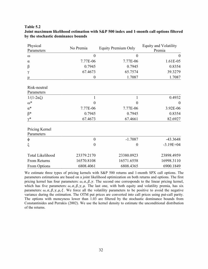
Table 5.1 presents the results for the estimation of the pricing kernels with 1-month S&P 500 call

options, while Table 5.2 presents the results from identical option data but those filtered by the

stochastic dominance bounds. Both the estimations indicate that the quadratic pricing kernel is

not fitting the data properly with the scaling factor (1

1−2𝛼𝜉< 1), while the results from the linear

pricing kernel do not show any magnitude problems as expected.

Comparing the results from the two tables, a number of the results are noteworthy. First, the

value of γ has changed a lot after the data filtering. γ controls the skewness or the asymmetry of

the distribution of the log-returns. The leverage effect, which is determined by the parameter, has

been much lower after we introduce the stochastic dominance bounds to the estimation. Also, the

estimations with stochastic dominance bounds are closer to the estimation results from asset

returns data only, in terms of the GARCH model parameters. It indicates the results presented by

Table 5.2 are more consistent with the physical dynamics, comparing with the results without

performing the stochastic dominance bounds. Finally, the likelihoods from both returns and

options have been increasing with regards to the three types of pricing kernels after filtering the

data. It can be viewed as an improvement of the kernel estimation given a better quality of the

options sample.

Although the estimations conducted with and without the stochastic dominance bounds are still

indicating a misfit of the data presented by the kernel estimation, the parameters estimated after

performing the bounds are better fit in magnitude. The mispriced options, which represent 14.04%

of the options sample, are strongly affecting the estimation results.

34

6 The Continuous-Time Heston Model

From previous sections, we observe perverse parameters from both the analytical formulations

and the empirical estimations under the GARCH framework. Because of the convergence from

the Heston-Nandi (2000) model to the Heston (1993) model in a continuous-time limit4 and also

their identical pricing kernel, it is important to test whether such a misfit of data is observable

from the continuous-time Heston model as well.

In Heston (1993), the price dynamics under stochastic volatility are:

𝑑𝑆(𝑡) = (𝑟 + 𝜇𝑣(𝑡))𝑆(𝑡)𝑑𝑡 + √𝑣(𝑡)𝑆(𝑡)𝑑𝑧1(𝑡)

𝑑𝑣(𝑡) = 𝜅(𝜃 − 𝑣(𝑡))𝑑𝑡 + 𝜎√𝑣(𝑡) (𝜌𝑑𝑧1(𝑡) + √1 − 𝜌2𝑑𝑧2(𝑡)),

where 𝑟 is the risk-free rate, 𝜇 governs the equity premium, while 𝑧1(𝑡) and 𝑧2(𝑡) are

independent Wiener processes.

The pricing kernel under the Heston model is equivalent to the GARCH pricing kernel with the

summation replaced by an integral:

𝑀(𝑡) = 𝑀(0) (𝑆(𝑡)

𝑆(0))

𝜙

𝑒𝑥𝑝 (𝛿𝑡 + 𝜂 ∫ 𝑣(𝑠)𝑑𝑠𝑡

0

+ 𝜉(𝑣(𝑡) − 𝑣(0))).

With the pricing kernel, the physical dynamics of Heston (1993) model are risk-neutralized to

𝑑𝑆(𝑡) = 𝑟𝑆(𝑡)𝑑𝑡 + √𝑣(𝑡)𝑆(𝑡)𝑑𝑧1∗(𝑡)

𝑑𝑣(𝑡) = (𝜅(𝜃 − 𝑣(𝑡)) − 𝜆𝑣(𝑡)) 𝑑𝑡 + 𝜎√𝑣(𝑡) (𝜌𝑑𝑧1∗(𝑡) + √1 − 𝜌2𝑑𝑧2

∗(𝑡)),

where 𝑧1∗(𝑡) and 𝑧2

∗(𝑡) denote two independent Wiener processes under the risk-neutral measure

Q. Given that the pricing kernel 𝑀(𝑡) is the only arbitrage-free specification that satisfies the

dynamics under both physical and risk-neutral distribution, CHJ (2013) solve the following

equations:

𝜇 = −𝜙 − 𝜉𝜎𝜌

𝜆 = −𝜌𝜎𝜙 − 𝜎2𝜉 = 𝜌𝜎𝜇 − (1 − 𝜌2)𝜎2𝜉.

4 See more details of the convergence in the appendix.

35

With such relations, we can interpret the equity risk premium 𝜇 and variance risk premium 𝜆

using the underlying risk-aversion parameter 𝜙 and the variance preference parameter 𝜉.

The equity premium and variance preference parameters (𝜙 and 𝜉) from the GARCH quadratic

pricing kernel, which are part of the parameter and volatility mappings, are directly involved in

the joint likelihood estimation. As a result, the two preference parameters from the continuous-

time pricing kernel are implied by the stochastic volatility model parameters:

𝜉 =𝜇𝜎𝜌 − 𝜆

𝜎2(1 − 𝜌2)

𝜙 =−𝜇 + 𝜆𝜎−1𝜌

1 − 𝜌2.

This results in a major difference between the continuous-time Heston model and the discrete-

time Heston-Nandi model as implied by the identical pricing kernel.

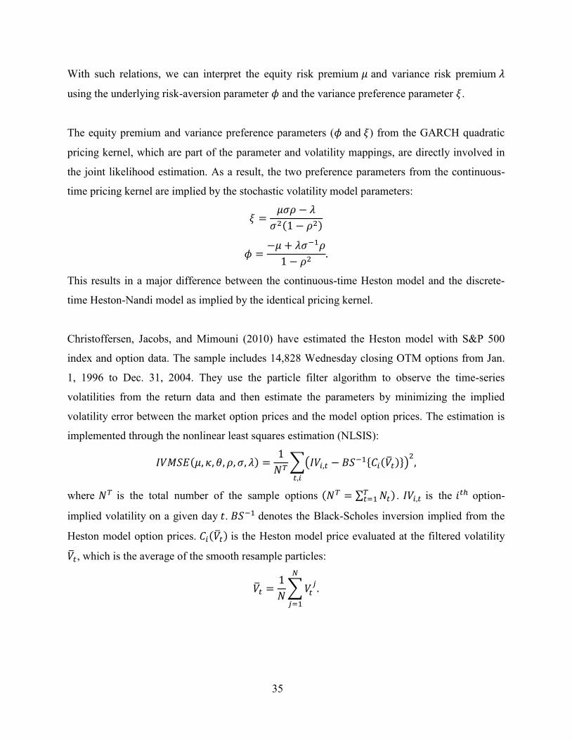
Christoffersen, Jacobs, and Mimouni (2010) have estimated the Heston model with S&P 500

index and option data. The sample includes 14,828 Wednesday closing OTM options from Jan.

1, 1996 to Dec. 31, 2004. They use the particle filter algorithm to observe the time-series

volatilities from the return data and then estimate the parameters by minimizing the implied

volatility error between the market option prices and the model option prices. The estimation is

implemented through the nonlinear least squares estimation (NLSIS):

𝐼𝑉𝑀𝑆𝐸(𝜇, 𝜅, 𝜃, 𝜌, 𝜎, 𝜆) =1

𝑁𝑇∑(𝐼𝑉𝑖,𝑡 − 𝐵𝑆−1{𝐶𝑖(�̅�𝑡)})

2

𝑡,𝑖

,

where 𝑁𝑇 is the total number of the sample options (𝑁𝑇 = ∑ 𝑁𝑡𝑇𝑡=1 ) . 𝐼𝑉𝑖,𝑡 is the 𝑖𝑡ℎ option-

implied volatility on a given day 𝑡. 𝐵𝑆−1 denotes the Black-Scholes inversion implied from the

Heston model option prices. 𝐶𝑖(�̅�𝑡) is the Heston model price evaluated at the filtered volatility

�̅�𝑡, which is the average of the smooth resample particles:

�̅�𝑡 =1

𝑁∑ 𝑉𝑡

𝑗

𝑁

𝑗=1

.

36

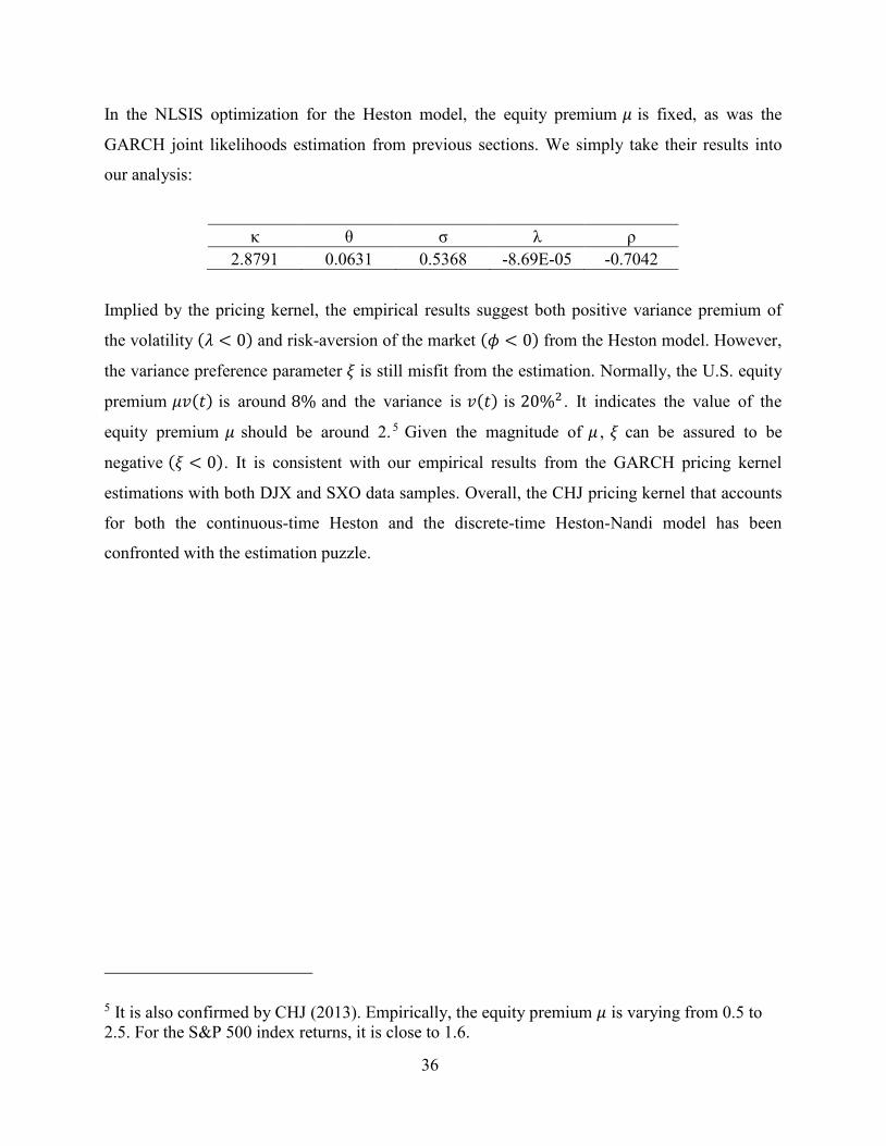
In the NLSIS optimization for the Heston model, the equity premium 𝜇 is fixed, as was the

GARCH joint likelihoods estimation from previous sections. We simply take their results into

our analysis:

κ θ σ λ ρ

2.8791 0.0631 0.5368 -8.69E-05 -0.7042

Implied by the pricing kernel, the empirical results suggest both positive variance premium of

the volatility (𝜆 < 0) and risk-aversion of the market (𝜙 < 0) from the Heston model. However,

the variance preference parameter 𝜉 is still misfit from the estimation. Normally, the U.S. equity

premium 𝜇𝑣(𝑡) is around 8% and the variance is 𝑣(𝑡) is 20%2 . It indicates the value of the

equity premium 𝜇 should be around 2. 5 Given the magnitude of 𝜇 , 𝜉 can be assured to be

negative (𝜉 < 0). It is consistent with our empirical results from the GARCH pricing kernel

estimations with both DJX and SXO data samples. Overall, the CHJ pricing kernel that accounts

for both the continuous-time Heston and the discrete-time Heston-Nandi model has been

confronted with the estimation puzzle.

5 It is also confirmed by CHJ (2013). Empirically, the equity premium 𝜇 is varying from 0.5 to

2.5. For the S&P 500 index returns, it is close to 1.6.

37

7 Concluding Remarks

This study estimates a GARCH option pricing model together with its quadratic pricing kernel

proposed by CHJ (2013). As motivated by a perverse estimation result from CHJ (2013), we

replicate the estimation with different data samples from both American and Canadian markets.

The new pricing kernel is still observed to misfit the data. We further examine the pricing kernel

under the continuous-time Heston model with the estimation results from Christoffersen, Jacobs,

and Mimouni (2010). The variance preference parameter is misfit as well. The newly developed

quadratic pricing kernel is confirmed to have the empirical puzzle.

In addition to the estimations, we compare the empirical performance of the linear pricing kernel

from the Heston-Nandi model to the quadratic pricing kernel from the CHJ model. Both the

pricing kernels have a good performance in the overreaction tests. However, the newly

developed pricing kernel is not able to outperform the linear pricing kernel.

We try to analyze the causes of the parametric magnitude problem. According to the quantitative

relations posted by the pricing kernel, either the risk-aversion parameter 𝜙 or the scaling factor

1/(1-2αξ) tends to be misfit. Also, we find the mispricing of the options would have an influence

on the estimation. There is a notable difference between the estimation results from the options

filtered by the stochastic dominance bounds and those from the unfiltered options. Part of the

failure would be contributed to the mispricing of the options.

38

Reference

Barone-Adesi, G., Mancini, L., & Shefrin, H. (2013). A tale of two investors: Estimating

optimism and overconfidence. Swiss Finance Institute Research Paper, (12-21).

Bates, D. (1996). Jumps and stochastic volatility: Exchange rate processes implicit in deutsche

mark options. Review of Financial Studies, 9(2), 69-107.

Bates, D. (2000). Post-'87 crash fears in the S&P 500 futures option market. Journal of

Econometrics, 94(1-2), 181-238.

Bates, D. (2003). Empirical option pricing: A retrospection. Journal of Econometrics, 116(1-2),

387-404.

Benzoni, L. (1998). Pricing options under stochastic volatility: An econometric analysis.

Manuscript, University of Minnesota.

Black, F., & Scholes, M. (1973). The pricing of options and corporate liabilities. The Journal of

Political Economy, 637-654.

Bollerslev, T. (1987). A conditionally heteroskedastic time series model for speculative prices

and rates of return. The Review of Economics and Statistics, 542-547.

Bollerslev, T., Chou, R. Y., & Kroner, K. F. (1992). ARCH modeling in finance: A review of the

theory and empirical evidence. A Review of the Theory and Empirical Evidence, 52(1), 5-59.

Breeden, D. T., & Litzenberger, R. H. (1978). Prices of state-contingent claims implicit in option

prices. The Journal of Business, 51(4), 621-651.

Brennan, M. (1979). The pricing of contingent claims in discrete time models. The Journal of

Finance, 34(1), 53-68.

Christoffersen, P., Heston, S., & Jacobs, K. (2013). Capturing option anomalies with a variance-

dependent pricing kernel. Review of Financial Studies, 26(8), 1963-2006.

Christoffersen, P., Elkamhi, R., Feunou, B., & Jacobs, K. (2010). Option valuation with

conditional heteroskedasticity and nonnormality. Review of Financial Studies, 23(5), 2139-

2183.

Christoffersen, P., Jacobs, K., & Mimouni, K. (2010). Volatility dynamics for the S&P500:

Evidence from realized volatility, daily returns, and option prices. Review of Financial

Studies, 23(8), 3141-3189.

39

Constantinides, G. M. (1979). Multiperiod consumption and investment behavior with convex

transactions costs. Management Science, 25(11), 1127-1137.

Constantinides, G. M., Jackwerth, J. C., & Perrakis, S. (2009). Mispricing of S&P 500 index

options. Review of Financial Studies, 22(3), 1247-1277.

Constantinides, G. M., & Perrakis, S. (2002). Stochastic dominance bounds on derivatives prices

in a multiperiod economy with proportional transaction costs. Journal of Economic

Dynamics and Control, 26(7-8), 1323-1352.

Constantinides, G. M., & Perrakis, S. (2007). Stochastic dominance bounds on american option

prices in markets with frictions. Review of Finance, 11(1), 71-115.

Cox, J. C., Ingersoll Jr, J. E., & Ross, S. A. (1985). A theory of the term structure of interest

rates. Econometrica, 53(2), 385-407.

Duan, J. C. (1997). Augmented GARCH (p, q) process and its diffusion limit. Journal of

Econometrics, 79(1), 97-127.

Duan, J. C., & Simonato, J. G. (1998). Empirical martingale simulation for asset prices.

Management Science, 44(9), 1218-1233.

Duan, J. (1995). The GARCH option pricing model. Mathematical Finance, 5(1), 13-32.

Duffie, D., Pan, J., & Singleton, K. (2000). Transform analysis and asset pricing for affine jump‐

diffusions. Econometrica, 68(6), 1343-1376.

Dumas, B., Fleming, J., & Whaley, R. E. (1988). Implied volatility functions: Empirical tests.

The Journal of Finance, 53(6), 2059-2106.

Dumas, B., Fleming, J., & Whaley, R. E. (1998). Implied volatility functions: Empirical tests.

The Journal of Finance, 53(6), 2059-2106.

Engle, R. F. (1982). Autoregressive conditional heteroscedasticity with estimates of the variance

of united kingdom inflation. Econometrica, 50(4), 987-1007.

Engle, R. F., & Ng, V. K. (1993). Measuring and testing the impact of news on volatility. The

Journal of Finance, 48(5), 1749-1778.

Eraker, B., Johannes, M., & Polson, N. (2003). The impact of jumps in volatility and returns. The


Garman, M. B. (1976). A general theory of asset valuation under diffusion state processes.

University of California, Berkeley. Working Paper.

40

Gerber, H. U., & Shiu, E. S. (1994). Option pricing by esscher transforms. Transactions of the

Society of Actuaries, 46(99), 140.

Heston, S. (1993). A closed-form solution for options with stochastic volatility with applications

to bond and currency options. Review of Financial Studies, 6(2), 327-343.

Heston, S., & Nandi, S. (2000). A closed-form GARCH option valuation model. Review of

Financial Studies, 13(3), 585-625.

Hull, J., & White, A. (1987). The pricing of options on assets with stochastic volatilities. The


Jackwerth, J. (2000). Recovering risk aversion from option prices and realized returns. Review of

Financial Studies, 13(2), 433-451.

Merton, R. C. (1971). Optimum consumption and portfolio rules in a continuous-time model.

Journal of Economic Theory, 3(4), 373-413.

Merton, R. C. (1977). An analytic derivation of the cost of deposit insurance and loan guarantees:

An application of modern option pricing theory. Journal of Banking & Finance, 1(1), 3-11.

Monfort, A., & Pegoraro, F. (2012). Asset pricing with second-order esscher transforms. Journal

of Banking & Finance, 36(6), 1678-1687.

Nelson, D. B. (1990). Stationarity and persistence in the GARCH (1, 1) model. Econometric

Theory, 6(03), 318-334.

Perrakis, S. (1986). Option bounds in discrete time: Extensions and the pricing of the American

put. Journal of Business, 59(1), 119-141.

Perrakis, S., & Ryan, P. (1984). Option pricing bounds in discrete time. The Journal of Finance,

39(2), 519-525.

Ritchken, P. H. (1985). On option pricing bounds. The Journal of Finance, 40(4), 1219-1233.

Ritchken, P. H., & Kuo, S. (1988). Option bounds with finite revision opportunities. The Journal

of Finance, 43(2), 301-308.

Rosenberg, V., & Engle, R. F. (2002). Empirical pricing kernels. Journal of Financial

Economics, 64(3), 341-372.

Rubinstein, M. (1976). The valuation of uncertain income streams and the pricing of options. The

Bell Journal of Economics, 7(2), 407-425.

Stein, E. M., & Stein, J. C. (1991). Stock price distributions with stochastic volatility: An

analytic approach. Review of Financial Studies, 4(4), 727-752.

41

Stein, J. C. (1989). Overreactions in the options market. The Journal of Finance, 44(4), 1011-

1023.

Stentoft, L. (2005). Pricing American options when the underlying asset follows GARCH

processes. Journal of Empirical Finance, 12(4), 576-611.

Taylor, S. J. (Ed.). (1986). Modelling financial times series. New York: Wiley.

Wiggins, J. B. (1987). Option values under stochastic volatility: Theory and empirical estimates.

Journal of Financial Economics, 19(2), 351-372.

42

Appendix

The convergence from the Heston-Nandi (2000) model to the Heston (1993) model

The physical dynamics from Heston and Nandi (2000) are:

ln(𝑆(𝑡)) = ln(𝑆(𝑡 − 1)) + 𝑟 + 𝜆ℎ(𝑡) + √ℎ(𝑡)𝑧(𝑡)

ℎ(𝑡) = 𝜔 + 𝛽ℎ(𝑡 − 1) + 𝛼 (𝑧(𝑡 − 1) − 𝛾√ℎ(𝑡 − 1))2

,

where 𝜆 = 𝜇 −1

2. We have the conditional mean and variance of ℎ(𝑡) given a lag ∆:

𝐸𝑡−∆[ℎ(𝑡 + ∆)] = 𝜔 + 𝛼 + (𝛽 + 𝛼𝛾2)ℎ(𝑡)

𝑉𝑎𝑟𝑡−∆[ℎ(𝑡 + ∆)] = 𝛼2(2 + 4𝛾2ℎ(𝑡)).

The instantaneous variance is defined by 𝑣(𝑡) = ℎ(𝑡)∆⁄ , while ℎ(𝑡) converges to zero under the

continuous-time limit. Following the GARCH process, 𝑣(𝑡) follows the dynamics:

𝑣(𝑡 + ∆) =𝜔

∆+ 𝛽𝑣(𝑡) +

𝛼

∆(𝑧(𝑡) − 𝛾√∆√𝑣(𝑡))

2

.

Assume 𝛼(∆) =1

4𝜎2∆2 , 𝛽(∆) = 0 , 𝜔(∆) = (𝜅𝜃 −

1

4𝜎2) ∆2 , 𝛾(∆) =

2

𝜎∆−

𝜅

𝜎, 𝜆(∆) = 𝜆 , the

following expectations are derived:

𝐸𝑡−∆[𝑣(𝑡 + ∆) − 𝑣(𝑡)] = 𝜅(𝜃 − 𝑣(𝑡))∆ +1

4𝜅2𝑣(𝑡)∆2

𝑉𝑎𝑟𝑡−∆[𝑣(𝑡 + ∆)] = 𝜎2𝑣(𝑡)∆ + (𝜎4

8− 𝜎2𝜅𝑣(𝑡) +

𝜎2𝜅2

4𝑣(𝑡)∆) ∆2.

Given the expectations, we can have the physical process of the Heston (1993) model:

𝑑 log 𝑆(𝑡) = (𝑟 + 𝜆𝑣(𝑡))𝑑𝑡 + √𝑣(𝑡)𝑑𝑧(𝑡)

𝑑𝑣(𝑡) = 𝜅(𝜃 − 𝑣(𝑡))𝑑𝑡 + 𝜎√𝑣(𝑡)𝑑𝑧(𝑡).

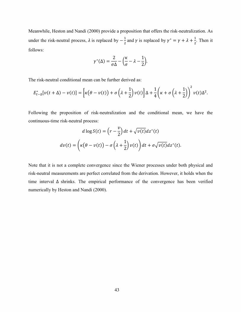
43

Meanwhile, Heston and Nandi (2000) provide a proposition that offers the risk-neutralization. As

under the risk-neutral process, 𝜆 is replaced by −1

2 and 𝛾 is replaced by 𝛾∗ = 𝛾 + 𝜆 +

1

2. Then it

follows:

𝛾∗(∆) =2

𝜎∆− (

𝜅

𝜎− 𝜆 −

1

2).

The risk-neutral conditional mean can be further derived as:

𝐸𝑡−∆∗ [𝑣(𝑡 + ∆) − 𝑣(𝑡)] = [𝜅(𝜃 − 𝑣(𝑡)) + 𝜎 (𝜆 +

1

2) 𝑣(𝑡)] ∆ +

1

4(𝜅 + 𝜎 (𝜆 +

1

2))

2

𝑣(𝑡)∆2.

Following the proposition of risk-neutralization and the conditional mean, we have the

continuous-time risk-neutral process:

𝑑 log 𝑆(𝑡) = (𝑟 −𝑣

2) 𝑑𝑡 + √𝑣(𝑡)𝑑𝑧∗(𝑡)

𝑑𝑣(𝑡) = (𝜅(𝜃 − 𝑣(𝑡)) − 𝜎 (𝜆 +1

2) 𝑣(𝑡)) 𝑑𝑡 + 𝜎√𝑣(𝑡)𝑑𝑧∗(𝑡).

Note that it is not a complete convergence since the Wiener processes under both physical and

risk-neutral measurements are perfect correlated from the derivation. However, it holds when the

time interval ∆ shrinks. The empirical performance of the convergence has been verified

numerically by Heston and Nandi (2000).

Documents

Volatility Risk and the Pricing Kernel in the Heston and ... · The Pricing Kernel in the Heston and Nandi (2000) and Heston ... the idea of pricing kernel is originally implicit