The Distribution of Average and Marginal Effective Tax

The Distribution of Average and Marginal Effective Tax Rates in European Union Member States.

Herwig Immervoll

University of Cambridge; European Centre for Social Welfare Policy and Research, Vienna

Abstract Macro-based summary indicators of effective tax burdens do not capture differences in effective tax rates facing different sub-groups of the population. They also cannot provide information on the level or distribution of the marginal effective tax rates thought to influence household behaviour. I use EUROMOD, an EU-wide tax-benefit microsimulation model, to compute distributions of average and marginal effective tax rates across the household population in fourteen European Union Member States. Using different definitions of ‘net taxes’ , the tax base and the unit of analysis I present a range of measures showing the contribution of the tax-benefit system to household incomes, the average effective tax rates applicable to income from labour and marginal effective tax rates faced by working men and women. In a second step, effective tax rates are broken down to separately show the influence of each type of tax-benefit instrument. The results show that measures of effective tax rates vary considerably depending on incomes, labour market situations and family circumstances. Using single averages or macro-based indicators will therefore provide an inappropriate picture of tax burdens faced by large parts of the population.

Keywords: Effective Tax Rates; European Union; Microsimulation. JEL Classification: H22; D31; C81 Address for correspondence: Department of Applied Economics University of Cambridge Sidgwick Avenue, Cambridge CB3 9DE, UK. e-mail: [email protected]

The Distribution of Average and Marginal Effective Tax Rates in the European Union.

Herwig Immervoll1

Draft Version (09-08-02). Please do not quote without author’s permission.

1. Introduction The analysis of most tax and transfer policy issues requires knowledge about how much is paid in taxes and received in benefits, by whom and in what circumstances. Moreover, in assessing existing tax-benefit policies and proposing reforms, it is useful to compare levels and structures of taxes and benefits across countries. The complexity of relevant rules governing tax liability and benefit entitlement and a lack of comprehensive and comparable data at the micro-level has led to major efforts being directed towards finding methods to construct simple summary indicators such as implicit effective tax rates based on revenue statistics and national accounts data (Carey and Tchilinguirian, 2000; Martinez-Mongay, 2000). While these measures can provide important insights regarding aggregate payments they cannot answer questions about their detailed incidence.2 Since they are normally derived

1 Research Associate at the Microsimulation Unit in the Department of Applied Economics, University of Cambridge and Research Fellow at the European Centre for Social Welfare Policy and Research, Vienna. Address for correspondence: Microsimulation Unit, Department of Applied Economics, University of Cambridge, Sidgwick Avenue, Cambridge, CB3 9DE, UK. Email: [email protected]. This paper was written as part of the MICRESA project, financed by the Improving Human Potential programme of the European Commission (SERD-2001-00099). I acknowledge the contributions of all past and current members of the EUROMOD consortium to the construction of the EUROMOD model. The views expressed in this paper as well as any errors are my own responsibility. In particular, this applies to the interpretation of model results and any errors in its use. EUROMOD is continually being improved and updated. The results presented here represent work in progress. EUROMOD relies on micro-data from 11 different sources for fifteen countries. These are the European Community Household Panel (ECHP) made available by Eurostat; the Austrian version of the ECHP made available by the Interdisciplinary Centre for Comparative Research in the Social Sciences; the Living in Ireland Survey made available by the Economic and Social Research Institute; the Panel Survey on Belgian Households (PSBH) made available by the University of Liège and the University of Antwerp; the Income Distribution Survey made available by Statistics Finland; the Enquête sur les Budgets Familiaux (EBF) made available by INSEE; the public use version of the German Socio Economic Panel Study (GSOEP) made available by the German Institute for Economic Research (DIW), Berlin; the Survey of Household Income and Wealth (SHIW95) made available by the Bank of Italy; the Socio-Economic Panel for Luxembourg (PSELL-2) made available by CEPS/INSTEAD; the Socio-Economic Panel Survey (SEP) made available by Statistics Netherlands through the mediation of the Netherlands Organisation for Scientific Research - Scientific Statistical Agency; and the Family Expenditure Survey (FES), made available by the UK Office for National Statistics (ONS) through the Data Archive. Material from the FES is Crown Copyright and is used by permission. Neither the ONS nor the Data Archive bear any responsibility for the analysis or interpretation of the data reported here. An equivalent disclaimer applies for all other data sources and their respective providers cited in this acknowledgement. All errors and views expressed are the responsibilities of the authors. 2 Throughout the paper, I use the terms tax and benefit payments to refer to the actual amounts paid in tax or received as benefits, i.e., the formal incidence. How this relates to the final (‘economic’ ) incidence is discussed in section 3.

2

by looking at monetary aggregates without considering the institutional rules as they apply to each taxpayer and benefit recipient, they also cannot capture the extents to which taxes and benefits affect incentives of people in different circumstances. This paper aims to fill these gaps by providing detailed measures of both average and marginal effective tax rates facing households in Europe. It uses an EU-wide microsimulation model (EUROMOD) to produce distributions of these measures across households in fourteen Member States of the European Union (EU). Effective tax rates capture the net tax burden resulting from the interaction of different types of taxes and contributions on one hand and benefit payments on the other. Average effective tax rates (AETRs) express the resulting net payments as a fraction of the income on which they are levied. They are therefore useful in assessing the size of transfers given the incomes and circumstances observed at a given point in time. Marginal effective tax rates (METRs), on the other hand, measure the degree to which any additional income would be ‘ taxed away’. METRs are therefore useful measures for evaluating the financial incentives to engage in activities meant to generate or increase income. The accurate measurement of AETRs and METRs is important for a range of policy related questions which continue to receive attention in both academic and policy circles. Measures of effective tax rates have, for instance, been used as explanatory variables in studies concerning the influence of tax burdens on economic growth (Agell, et al., 1997; , 1999), unemployment (Daveri and Tabellini, 2000; Martinez-Mongay and Fernández-Bayón, 2001) and wage setting behaviour (Sorensen, 1997). Clearly, many of the processes underlying these issues are strictly linked to the behaviour of individuals or households. In comparing and evaluating different tax-benefit systems one would therefore want to characterise them not only in terms of the effective tax burden of a single ‘ representative’ agent3 but also in terms of the number and types of households and individuals who are, in fact, facing effective tax rates of the various magnitudes. In fact, from a distributional point of view, detailed knowledge about the incidence of tax and benefit payments is of interest in itself (e.g., Mercader-Prats, 1997). Although comparable and detailed household micro-data have become more readily available in recent years, the information contained in these data sources is nevertheless insufficient for calculating detailed AETRs and METRs. One reason is simply that variables on income tax (IT) or social insurance contributions (SIC) are often missing. Even if they are recorded, social insurance contributions paid by employers (or benefit paying institutions) on behalf of employees will usually not be available (as shown below, employers’ contributions represent an important part of the tax burden borne by labour incomes). To overcome this problem simulation methods are frequently used to impute such missing information (Immervoll and O'Donoghue, 2001a; Weinberg, 1999). This basically entails combining the information on people’s status and incomes with a detailed representation of tax-benefit rules and provides all necessary information for computing AETRs. The incorporation of detailed tax-benefit rules in microsimulation models has two other distinct advantages. They allow analysts to evaluate the effects on tax and benefit amounts of 3 This is, in effect, what effective tax rate measures based on macro-data do.

3

changes of either the tax-benefit rules or the characteristics of households. The latter is necessary in order to compute METRs. By varying each observation’s incomes by a certain amount and then re-computing tax liabilities and benefit entitlements, the effective tax burden on any additional income can be captured. Secondly, effective tax rates can be computed under a range of different policy configurations. In the EU, such ‘ forward-looking’ analyses of the likely impact of policy reforms on effective tax burdens are particularly relevant given the identification of ‘high’ or ‘excessive’ levels of taxation as a major policy concern.4 The plan for this paper is as follows. Section 2 provides a rationale for evaluating effective tax rates at the micro-level and compares approaches using empirical micro-data to macro-based techniques as well as methods based on ‘synthetic’ households. Section 3 discusses the choices to be made in measuring effective tax rates and explains the precise approach adopted in the present study. The following sections present simulation results for fourteen countries. While section 4 provides household-level AETRs across all households taking into account all relevant taxes and benefits, section 5 focuses on the effective taxation of labour incomes. It presents individual-level estimates of the total tax ‘wedge’ resulting from the combination of IT and SIC. Section 6 evaluates relevant financial incentives for the working population by computing METRs. All results are presented in terms of their overall distribution of effective tax rates across the relevant populations as well as grouping by age, gender and other household characteristics. In discussing policy reforms targeted towards altering effective tax rates it is essential to understand which particular tax-benefit instruments are responsible for observed tax burdens. The distributions of METRs and AETRs are therefore decomposed in order to show the contributions of individual tax-benefit instruments. Section 7 concludes. 2. Measuring effective tax rates – why look at the micro-level? International comparisons of tax systems have long relied on information about formal tax rules (such as the rate structure) or they have summarised their aggregate impact by relating total receipts to national income (these indicators are sometimes called ‘ tax ratios’). One main shortcoming of this latter approach is that it disregards the tax base a tax is levied on. A ‘ tax ratio’ for a certain type of income tax of x% may be the result of a combination of (a) a broad tax base and a low tax rate; or (b) a narrow tax base and a high tax rate. The economic consequences are, obviously, very different. To rectify this problem, there has, starting in the 1990s, been a growing interest in methods seeking to derive measures of effective tax rates based on Revenue Statistics and National Accounts (Lucas Jr, 1990, Mendoza, et al., 1994). By relating tax receipts to the relevant tax bases they provide a much better indicator of tax burdens. They are also attractive in that deriving comparable figures across countries is facilitated by the availability of internationally comparable sources of revenue statistics, such as those produced by the OECD, and standardised national accounts data. Obviously, macro-based measures cannot be used to investigate the micro-level incidence of tax payments. There are, however, other potential problems. One is related to the institutional characteristics in terms of how taxes and benefits are integrated in different countries and the fact that macro-based effective tax rates tend to focus on taxes and SIC while disregarding

4 In 2000 the European Council has, for instance, committed the European Commission to assess “whether adequate measures are being taken in order to […] alleviate the tax pressure on labour […]” (Martinez-Mongay (2000), p. 6). Carone and Salomäki (2001) supply a recent contribution towards such an assessment.

4

benefits. Child related payments may, for instance, be formally administered through the tax system in some countries (e.g., by means of refundable tax credits) and be paid as benefits in others. Clearly, excluding benefit payments in such cases means that the comparability of effective tax rates across countries will suffer. While, in principle, applying appropriate corrections would be straightforward, data on social transfers tends to be less comparable across countries than revenue statistics and incorporating them in multi-country studies can therefore be problematic. Technical difficulties also arise due to conceptual differences between revenue statistics and national accounts data. The former are, for instance, collected on a cash basis while the latter measure incomes as they accrue. As a result the timing of the two data sources diverges (Jacobs and Spengel, 1999). Several other issues are also related to differences in definitions and scope between the two data sources and a number of assumptions are required to align them (Carey and Tchilinguirian, 2000). This range of potential problems has prompted a number of ‘health warnings’ being issued in order to make users of macro-based effective tax rates aware of their shortcomings (OECD, 2000b; c). The Working Party No. 2 on Tax Policy Analysis and Tax Statistics of the OECD Committee on Fiscal Affairs takes the view that “AETR results relying on aggregate tax and national accounts data are potentially highly misleading indicators of relative tax burdens and tax trends” and that “ further work relying on micro-data is required to assess the magnitude of potential biases to average tax rate figures derived from aggregate data.”5 In fact, there is an existing literature documenting various approaches of combining information on statutory tax rules and tax returns with data on income distribution and household surveys (Barro and Sahasakul, 1986; Easterly and Rebelo, 1993). Among researchers interested in the macroeconomic effects of taxation, however, these attempts have been met with some scepticism (although some authors have in fact used them as yardsticks for validating macro-based results) as it is considered doubtful whether “marginal tax rates that apply to particular individuals in a household survey, or a specific aggregation of incomes based on tax-bracket weights, are equivalent to the aggregate tax rates that affect macroeconomic variables as measured in national accounts.”6 This limitation certainly holds for tax rate calculations based on ‘ typical’ households (such as OECD, 2000a) as such estimates, while illustrative, fail to take into account the heterogeneity of the population. Although extending these calculations to a wider range of ‘synthetic’ households can serve to improve our understanding of the mechanics built into tax-benefit systems the point remains that any calculations based on synthetic households cannot capture, in the correct proportions, the tax and benefit payments across the entire range of household types found in the population as a whole (Immervoll, et al., 2001). In contrast, calculations based on representative household micro-data can be used to derive aggregate measures of effective tax rates using any desired aggregation rule. At the same time, they are more informative than aggregate measures since they capture the distribution of effective tax rates across the population.

5 Carey and Tchilinguirian (2000), p. 5. 6 Mendoza, et al. (1994), p. 2

5

As they are calculated based on statutory tax and benefit rules they are also particularly useful where a detailed knowledge of the structure and mechanics built into tax-benefit systems is important. There are two main cases where computing measures based on observed past tax receipts and tax bases (sometimes referred to as ‘backward-looking’ in the literature) cannot be used. First, measuring METRs requires assessing what would happen to tax burdens if incomes were to change. As tax-benefit systems are generally far from proportional, aggregate income changes are meaningless in this context. Instead, it is important whose income is changing. In a non-proportional tax-benefit system, METRs can therefore only be computed based on a knowledge of the distributions of incomes and other characteristics that determine tax liabilities and benefit entitlements. This problem is usually acknowledged in studies using macro-based measures of effective tax rates. However, since many of the distortionary effects of taxation that researchers are interested in are related to marginal rather than average tax rates, there is a worrying tendency to equate METRs with AETRs and use the latter as proxies for the former (see Mendoza, et al., 1994 for an example and Padovano and Galli, 2001 for a critique). A second area where ‘ forward-looking’ methods of computing effective tax rates are particularly useful is in the analysis of policy reforms. There is often a need to evaluate reforms before detailed macro-economic data become available. Since the delays can be sizable simulation techniques can play an important role in an early evaluation of policy reforms.7 By changing the parameters of the tax-benefit rules built into such simulation models, they can also be used to perform analyses of hypothetical or prospective reforms. 3. Whose taxes, which incomes, what margins? Several choices have to be made when measuring effective tax rates. Most of them have important implications for the interpretation of the results and thus require some consideration. In fact, depending on the research questions it will often be desirable to compute effective tax rates in several different ways. A method which allows some flexibility is therefore valuable. Before discussing the various decisions to be made and how microsimulation methods can be used to accommodate them it is useful to clarify the scope of the measurement exercise. AETRs measure some concept of total tax as a fraction of some concept of tax base. Obviously, the incidence of AETRs is therefore connected with the incidence of taxes. In studying questions of incidence one can be interested in the payments per se, or in the economic loss suffered by the taxpayer. For a particular taxpayer, this loss will, for two reasons, generally differ from the tax paid. First, taxes may, through influences on supply and demand at the market level, influence the prices of the goods and service produced or consumed by the taxpayer. Second, the taxpayer herself may, in response to price changes, adjust the basket of goods and service she produces or consumes and suffer welfare losses in the process. The familiar process of tax ‘shifting’ is of great interest to economists and any results on final incidence may be very sensitive to the degree of shifting.8

7 Martinez-Mongay (2000) notes that there is generally a 2-3 year lag in the production of macro-based tax rates. 8 Indeed, imperfect competition may lead to over-shifting in the sense that the loss suffered by a taxpayer can be less than 0% or more than 100% of the amount of tax paid. See, for instance, Stern (1987).

6

Moreover, there are many economic consequences of taxation that cannot be captured by looking at the amounts of taxes alone. To take an extreme example, a tax that, at a given point in time, generates no revenue at all may be detrimental to economic growth if it has made a certain type of productive activity so financially unattractive as to drive people away from engaging in it altogether. Nevertheless, it is difficult to deny that tax payments are an issue of public interest in themselves and therefore deserve investigation. The central issue then is to “distinguish clearly between tax payments and losses from taxation, and to recognise that the first is an accounting characteristic of a particular equilibrium, while the second requires the evaluation of a comparison between two alternative equilibria.” 9 In this paper, effective tax rates are computed for a given ‘equilibrium’ as characterised by the information recorded in household micro-data of a particular year. While the resulting AETRs will, for the reasons stated above, not capture total losses associated with the imposition of taxes, any substitution effects caused by them do enter the results: If we assume that we are, in fact, looking at an equilibrium then people will already have adjusted their activities in response to the tax burdens imposed on them.10 The aim of computing AETRs is to understand the extent and incidence of burdens resulting from tax payments and, to avoid confusion, there should be no claim that the incidence of AETRs can be used as some sort of approximation of the incidence of economic losses (relative to the tax base). Instead, tax payments are one component of incidence analyses and should be treated as such.11 For METRs, on the other hand, no qualifications regarding any decisions about the appropriate treatment of tax shifting are required at all. The main reason why we are interested in METRs in the first place is their possible effect on behaviour or, in other words, their role in moving from ‘equilibrium 1’ to ‘equilibrium 2’ . Clearly, METRs must therefore be evaluated under ‘equilibrium 1’ . While some of the methodological issues to be considered for effective tax rate measurement at the micro-level are similar or can at least be related to those facing researchers concerned with deriving macro-based measures, others only become apparent due to the level of detail which micro-based approaches support. Even though these issues exist, in principle, regardless of the level of aggregation, the data sources used for macro-based measures simply do not provide the same range choices. The relevant dimensions are (1) the types of taxes and benefits to take into account and the income (or ‘tax base’) to relate them to and (2) the unit of analysis and, related to it, the sharing of any incomes within the unit. In the case of METRs an additional issues is (3) the nature and size of the margin to be used for computing marginal effects. Each of these will be discussed in turn.

9 Dilnot, et al. (1990), p. 213. 10 It should be emphasised that this implies an important qualification of studies looking at effects of policy reforms on the incidence of effective tax rates. If taxes and benefits are computed for a given (pre-reform) population then, conceptually, the assumption of an equilibrium will not be appropriate. To what extent taking into account behavioural responses following the reform would, in fact, noticeably change results is another matter. The usefulness of incorporating behavioural response in microsimulation-based policy evaluations will depend on the precise type and intent of the reform and on the extent to which underlying micro-data permit changes to be detected in a statistically meaningful way. For a discussion of some of these and related issues see Pudney and Sutherland (1994) and Creedy and Duncan (2002). 11 Dilnot, et al. (1990) show how tax payments, income effects due to price changes and welfare loss as a result of substitution processes can be brought together in one unified framework.

7

3.1 Tax-benefit instruments and definition of income base Although effective tax rates are supposed to provide broad measures of net tax payments, the choice of instruments to be incorporated in such a measure is not self-evident. Most studies consider taxes and ‘ tax-like’ payments. However, it is not at all clear that SIC are, for example, equivalent to income taxes and it is undoubtedly the case that the degree of equivalence differs widely across countries. While, in principle, SIC are payments made in return for insurance coverage the link between income taxes and public services is not as direct. However, cross subsidies between the various ‘pots’ of public finances often make such a distinction less meaningful. In addition, social insurance schemes are, for the most part, compulsory and not characterised by a strict actuarial link between the value of insurance services and SIC paid. The discrepancy can be seen as performing functions (such as redistribution or raising revenues) normally associated with income tax. Section 2 has already hinted at comparability problems that can arise due to international differences in the structure of tax-benefit systems when the benefit side is ignored. As the distinction between tax concessions and benefits is more or less arbitrary, tax-benefit models which allow an integrated view on the tax-benefit system as a whole are useful in this respect. There are, however, limitations nonetheless as these models usually focus on cash instruments. As a result, there are inherent difficulties in comparing effective tax rates of countries where, say, child care payments or housing benefits are paid an cash and those where these benefits are provided ‘ in-kind’ through access to subsidised child-care or housing. A related question is that about the appropriate time-horizon of the calculations. Should some measure of future benefits financed by current SIC be taken into account? Many of these issues become somewhat clearer once one considers the appropriate definition of income which is to enter the denominator of the AETR calculations. If the purpose of studying the incidence of AETRs is assessing the distribution of the relative contribution of tax-benefit systems to current cash incomes (as in section 4) then any in-kind transfers as well as future incomes such as pension rights will be disregarded.12 Similarly, if the focus is on evaluating the total tax burden on labour (as in section 5) then any taxes or benefits which are not strictly related to labour income (such as taxes on investment income, family benefits13) should be disregarded. 3.2 Unit of analysis and sharing within units A natural question to ask is whose effective tax rates we are interested in. Depending on the purpose, we may want to look at tax/benefit payments at the individual level, the level of the formal tax unit or some other notion of family or household. For distributional studies concerned with household welfare the household level will be appropriate (Canberra Group, 2001). In measuring the tax wedge on labour, however, one would want to relate the relevant 12 There would still be an issue of what ‘current’ means. Normally, income distribution studies take the year as their reference period (Canberra Group (2001)). In the context of effective tax rate calculations based on micro-data, this means that annual income data would be ideal. Some data sources, however, measure income over a shorter period (see appendix 1). Although these data can, of course, be annualised, time-period differences in the original data need to be borne in mind in comparative studies as income changes during the year will, for a particular household, imply that annual income is not equal to one particular month’s income times 12. 13 As illustrated by the ‘ tax concessions versus benefits’ example in section 2, the treatment of benefits is not always straightforward. If family related tax concessions in country A are allowed to reduce effective tax rates then, for symmetry reasons, the same may need to hold for family benefits in country B.

8

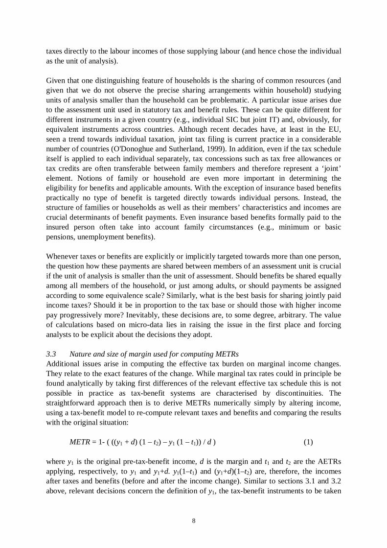
taxes directly to the labour incomes of those supplying labour (and hence chose the individual as the unit of analysis). Given that one distinguishing feature of households is the sharing of common resources (and given that we do not observe the precise sharing arrangements within household) studying units of analysis smaller than the household can be problematic. A particular issue arises due to the assessment unit used in statutory tax and benefit rules. These can be quite different for different instruments in a given country (e.g., individual SIC but joint IT) and, obviously, for equivalent instruments across countries. Although recent decades have, at least in the EU, seen a trend towards individual taxation, joint tax filing is current practice in a considerable number of countries (O'Donoghue and Sutherland, 1999). In addition, even if the tax schedule itself is applied to each individual separately, tax concessions such as tax free allowances or tax credits are often transferable between family members and therefore represent a ‘ joint’ element. Notions of family or household are even more important in determining the eligibility for benefits and applicable amounts. With the exception of insurance based benefits practically no type of benefit is targeted directly towards individual persons. Instead, the structure of families or households as well as their members’ characteristics and incomes are crucial determinants of benefit payments. Even insurance based benefits formally paid to the insured person often take into account family circumstances (e.g., minimum or basic pensions, unemployment benefits). Whenever taxes or benefits are explicitly or implicitly targeted towards more than one person, the question how these payments are shared between members of an assessment unit is crucial if the unit of analysis is smaller than the unit of assessment. Should benefits be shared equally among all members of the household, or just among adults, or should payments be assigned according to some equivalence scale? Similarly, what is the best basis for sharing jointly paid income taxes? Should it be in proportion to the tax base or should those with higher income pay progressively more? Inevitably, these decisions are, to some degree, arbitrary. The value of calculations based on micro-data lies in raising the issue in the first place and forcing analysts to be explicit about the decisions they adopt. 3.3 Nature and size of margin used for computing METRs Additional issues arise in computing the effective tax burden on marginal income changes. They relate to the exact features of the change. While marginal tax rates could in principle be found analytically by taking first differences of the relevant effective tax schedule this is not possible in practice as tax-benefit systems are characterised by discontinuities. The straightforward approach then is to derive METRs numerically simply by altering income, using a tax-benefit model to re-compute relevant taxes and benefits and comparing the results with the original situation:

METR = 1- ( ((y1 + d) (1 – t2) – y1 (1 – t1)) / d ) (1) where y1 is the original pre-tax-benefit income, d is the margin and t1 and t2 are the AETRs applying, respectively, to y1 and y1+d. y1(1–t1) and (y1+d)(1–t2) are, therefore, the incomes after taxes and benefits (before and after the income change). Similar to sections 3.1 and 3.2 above, relevant decisions concern the definition of y1, the tax-benefit instruments to be taken

9

into account in computing t1 and t2, as well as the unit of analysis used for measuring incomes. In addition, the size (and direction) of d is important and leads to different interpretations of resulting METRs. In establishing work incentives, one will often be interested in a small income change, such as a small fixed percentage rise in earnings or the rise in gross earnings due to an additional hour of work. However, the margin can also be earnings as a whole. 1-METR is then equivalent to the concept of a replacement rate (of moving from in-work to out-of work in the case of d = -earnings and out-of-work to in-work in the case of d = potential earnings). For such ‘ large’ margins, however, it is often not sufficient to only change income before re-computing taxes and benefits. In addition, several other characteristics which are available in the micro-data and which, in addition to income, are potential determinants of taxes and benefits (variables such as hours of work, employment status, economic sector) will have to be altered as well (see Immervoll and O'Donoghue, 2001c). If one is concerned with financial incentives then the appropriate choice of a unit is particularly important. If a persons’s additional earnings reduce the household’s entitlement to housing benefits then this is likely to be a consideration she will take into account. Similarly, an important consequence of joint taxation of married couples is that, from the couple’s point of view, the lower earning spouse faces, for a lower level of earnings, the same marginal tax rate as his/her higher earning partner. Clearly, to bring out these facts, METRs would need to be computed for the relevant unit as a whole. For multi-person units, however, another decision to be made is who to attribute d to. Since for the unit as a whole, METRs will be different depending on who earns the additional amount, it will often be appropriate to evaluate different scenarios. For example, in order to separately analyse financial work incentives for men and women one may analyse METRs evaluated for the household as a whole under the alternative assumptions that female / male members of household increase their earnings (see section 5). 4. The contribution of tax-benefit systems to households’ current disposable incomes Average effective tax rates can provide a convenient description of the degree to which household incomes are affected by taxes and benefits. The household perspective allows one to put aside issues related to the unit of analysis as discussed in section 3.2. The concern with current incomes also makes redundant any questions about the degree to which current taxes or SICs can be seen as savings financing future benefits. But an important consideration that remains is which components of current income should be counted in the numerator and denominator of the AETR. For most components such as earnings, taxes, SIC, family benefits, etc., the decision is straightforward. It is less clear-cut, however, for incomes which are partly insurance based but are also characterised by some elements of outright transfers to the recipient household. In cross-country studies, the issue is complicated by the fact that, for similar policy instruments, the “mix” between insurance and transfers varies widely across countries. This is particularly the case for pensions and unemployment benefits. For the purpose of this section, I consider all replacement incomes, such as old-age pensions and unemployment benefits, whether contributory or not, part of the tax base (i.e., pre-tax-benefit income) and not as benefits that reduce the net taxes paid by households. The AETRs

10

for recipients of these incomes therefore do not reflect the generosity of these instruments but the extent to which they are subject to (net) tax payments. Other replacement incomes which enter the tax base include maternity benefits, sickness benefits, disability insurance and survivor/orphan benefits. SIC paid by the employer are not part of pre-tax-benefit income. The denominator of the AETR consists of all taxes paid by the household plus compulsory own SIC minus family benefits, care benefits, social assistance/minimum income benefits and all other ‘non-replacement’ cash transfers such as housing benefits. For each household, the relevant income components are either taken directly from the micro-data (earnings, pensions, etc.) or simulated using EUROMOD, an EU-wide tax-benefit model. The sources of micro-data used in this exercise are listed in appendix 1. The same micro-data are also used by EUROMOD as the basis for simulating income taxes, SIC as well as means-tested and universal benefit payments. A simulation of these income components is necessary in cases where they are not recorded in the micro-data. In addition, simulation is required in order to compute changes in taxes and transfers following marginal income changes (section 6). EUROMOD is an integrated microsimulation model of the tax-benefit systems of all fifteen EU Member States. It permits common definitions of income concepts, units of analysis, sharing ‘ rules’ , etc. to be used across countries and therefore is a suitable instrument for computing effective tax rates in a comparable or, at least, reconcilable way.14 The tax and benefit rules underlying all calculations in this paper are those for 1998. Table 1 shows the distribution of household AETRs for fourteen countries along with the number of observations for each AETR band (modal values are shown in bold typeface). Large difference between median and mean in some countries are a first indication of the spread of AETRs across the population. While the amount of taxes and own SIC paid in the country as a whole is, relative to pre-tax-benefit income, similar in Ireland and the UK, the median is very different: half of Irish households pay less than 6% in net taxes with just under 20% having their incomes entirely unaffected by the tax-benefit system. The mean average effective tax burden on pre-tax-benefit income including replacement incomes is highest in Denmark and, at about a third of the Danish level, lowest in the UK, Ireland and Spain. Taking a closer look at the distribution we see that a considerable number of households are net benefit recipients with between 8% in Denmark and 30% in the UK having negative AETRs. For this group, non-replacement incomes exceed pre-tax benefit incomes. The fact that Denmark and the UK are the two extremes in this respect is instructive as one would a priori expect Denmark to have a more generous social transfer system. In interpreting these results it important to keep in mind that AETRs depend on both net-taxes and pre-tax-benefit incomes. If in a given country, there are more households where all household members are benefit recipients, we will therefore see a larger number of negative AETRs even if the benefits are less generous. Equally important, counting replacement incomes as pre-tax-benefit incomes will tend to push AETRs upwards for those countries with generous unemployment benefits and/or pensions: If people are entitled to these payments they will obviously be less likely to fall back on ‘ last-resort’ benefits such as social assistance or other means tested transfers.

14 Details on EUROMOD and the simulated tax-benefit instruments can be found in Immervoll, et al. (1999), Sutherland (2001b) and Immervoll and O'Donoghue (2001b).

11

Given the dissimilar distributions it is interesting to analyse which household characteristics are related to the level of AETRs. The interaction of the various characteristics of interest could be captured using regression techniques. I defer this approach to future work and instead show as a first step tables focussing on one characteristic at a time. Table 2 shows how the distributions differ for different income groups.15 While in the UK the tax burden borne by the top quintile is one of the lowest, this country also has the most ‘progressive’ system in that the average AETR in the top quintile is more than 100 percentage points higher than that for the bottom 20%. This does, of course, not mean that the mechanisms built into the tax-benefit system are in themselves necessarily more ‘progressive’ than in other countries. An important factor behind these numbers is the distribution of pre-tax-benefit incomes: More unequal distributions will, for a given structure of tax-benefit system, also result in larger disparities between effective tax burdens. In particular, if low-income groups draw a very large part of their income from social transfers (UK, Finland, Greece) then AETRs can be highly negative, leading to large percentage point differences when compared to AETRs of higher income groups.16 One main factor determining pre-tax-benefit incomes is the labour market status of household members. Table 3 considers two of the relevant groups; those economically “active” (employed or self-employed) and the retired. Since AETRs are computed here on a household basis the status refers to that of the head of household.17 For the groups as a whole, net taxes relative to pre-tax-benefit incomes are at least twice as high for the ‘active’ group in nine out of fourteen countries. In Ireland and Portugal the majority of households headed by a retired person do in fact face zero AETRs and are, thus, outside the scope of the tax-benefit system. While this is not the case in the UK, the mean AETR for retired people is negative indicating a large number of retired people with low pensions who are dependent on minimum income and other means-tested benefits. A large number of negative AETRs is also found among the retired group in Finland. Turning to the ‘active’ group the largest incidence of high AETRs is found in Denmark, Germany, the Netherlands and Belgium where, respectively, more than 89%, 49%, 41% and 40% of ‘active’ households are faced with AETRs in excess of 30%. The relevant proportion in the UK (2.5%) is the lowest of all fourteen countries followed by Spain with just under 4%. Table 4 shows separate distributions for different age groups (referring, again, to the head of household) and confirms the picture of clearly lower AETRs applying to those drawing their main income from old-age pensions. One can again see a large number of zero AETRs among the ‘>65’ households in Ireland and Portugal and also Spain. Along the age profile, AETRs in all countries follow an inverted ‘U’ shape which is particularly pronounced in Finland, Germany, Greece and the UK. The largest number of net benefit recipients among households headed by young (<25) people can be found in the Netherlands followed by the UK, Finland

15 In computing quintile points, differences in household size and composition have been corrected for using the ‘modified OECD’ equivalence scale. In dividing the population into five equally sized groups, households have been weighted by their size. 16 It is instructive that, in the UK, the difference in means between the top quintile group and the first quantile with non-negative mean AETRs (quintile group 3) is one of the lowest among the fourteen countries. 17 The ‘head of household’ is defined as the person with the highest earnings; if there is more than one person with the same (or zero) earnings, the oldest person is assumed to be the ‘head’ .

12

and Germany. A final breakdown of household AETRs is provided in table 5 where distributions are presented for a range of family structures. Single parent households are subject to lower effective tax rates than the overall population in all countries. With negative medians, they are mainly net benefit recipients in seven out of fourteen countries (Belgium, France, Germany, Ireland, Luxembourg, the Netherlands and, most clearly, the UK). Again, this may be due to generous benefits being available to them (such as in Belgium18) or to a lack of earning opportunities forcing them to rely on social transfers (whatever their level) or a combination of the two. Upon first inspection it may be surprising that households without children face lower AETRs than those with children in some countries (Greece, Italy, Portugal and Spain, in particular). This is to a large extent due to retired people being part of the ‘no children’ group. Once they are excluded (column ‘No Children; Head not retired’ ) households with children face lower AETRs than those without in all countries but Spain where a small difference in favour of childless households remains. How important are individual tax-benefit instruments in determining effective tax burdens? To answer this question, the various levels of AETRs in all countries have been decomposed in terms of the instruments that drive them. The results are shown in figure 1 where the contribution of each instrument to the total net taxes is shown for the different AETR bands.19 The bars all have the same total height (100%) so that a similar sized ‘ tax’ section in AETR bands ’40 to 45’ and ’20 to 25’ would, for instance, indicate an average amount of income tax in the former band being about twice as large as that in the latter band. Negative components (benefits) are those which reduce net taxes in each AETR band. Note that bars have been omitted for AETR bands with fewer than 10 observations. Except for that, however, the graphs say nothing about the incidence of the various AETR levels so that it is important to read them in conjunction with table 1. In addition to the contribution of individual tax-benefit instruments figure 1 graphs, for each AETR band, average per-capita ‘ tax-bases’ (i.e., pre-tax-benefit income including replacement incomes) relative the population median.20 As expected, higher tax-bases are generally subject to higher AETRs. As in table 2, however, the degree of progressivity varies across countries. Notably, we see that in four of the countries (Belgium, Greece, Italy, Spain, UK) the highest AETRs are not paid by those with the highest ‘ tax-base’. This is frequently due to upper contribution limits above which no (additional) SIC are due. However, taxes other than income tax (wealth and property tax) also play a role as these may lead to high total tax burdens relative to income. The balance between taxes and SIC as revenue generating instruments differs widely. In Denmark, Finland and the UK taxes represent, throughout the AETR spectrum, more than 75% of total household payments to the government. At the other extreme, own SIC paid by Austrians markedly exceed taxes in most AETR bands. On the benefit side, we see family benefits being a particularly important contributor to net benefit receipts of low-income households in Luxembourg, Spain, Italy and Belgium. The dependence of low-income households on minimum income benefits is strongest in Greece and Ireland while housing related cash benefits play an important role in this respect in the UK, France and Germany. In Denmark 18 See Immervoll, et al. (2001). 19 ‘Other Benefits’ are care benefits, educational grants and other transfers that do not fit into any of the other three benefit categories. As before, replacement incomes such as pensions or unemployment benefits are not counted as ‘benefits’ here but included in the ‘ tax base’ . 20 Per-capita levels have, again, been derived using the ‘modified OECD’ equivalence scale.

13

and the Netherlands, housing benefits are, as a fraction of total net taxes, largest for households with pre-tax-benefit incomes above about 40% of the median while for lower-income groups they are less important. 5. The effective tax burden on labour income The focus in this section is on the tax burden borne by labour incomes. As briefly discussed above this means that AETRs need to be evaluated for the individuals supplying the worked hours. It also requires a different definition of ‘net taxes’ and ‘ tax base’ than the exercise in section 4. First, although we are, again, only concerned with payments rather than the total ‘ losses’ they give rise to, it should not matter who pays the taxes formally.21 As a result, employer SIC paid on behalf of the employee are included in the numerator of the AETR ratio along with own SIC and income taxes. Since it is the burden on total labour income we are interested in employer SIC also need to be added to employment income to yield the ‘ tax base’ denominator.22 As a rule, benefits are not subtracted from the numerator. An exception are in-work benefits in the UK (Family Credit in 1998; now Working Families’ Tax Credit) which constitute a tax concession particularly designed to increase net labour incomes.23 An interesting conceptual question concerns the treatment of consumption taxes. Traditionally, it has been argued that, as they also reduce earners’ consumption opportunities, they need to be included in calculations of the ‘ labour tax wedge’ by adding them to the AETR numerator.24 However, a contrasting view is that, since consumption taxes apply to both earners and non-earners, they do not constitute a ‘ labour tax wedge’ and therefore do not matter for studying the relationship of tax burdens and unemployment (Daveri and Tabellini, 2000). In the results presented here, I implicitly adopt the second view as, for technical reasons, it is difficult to include consumption taxes in the fourteen country simulation exercise.25 Since AETRs are computed at an individual level rather than for the household as a whole it is necessary to assume sharing arrangements for joint income taxes. In this exercise, it is assumed that any joint income tax burdens of a joint tax unit are shared in proportion to

21 There is, however, a long-running debate whether SIC paid by employers have a stronger or more immediate effect on labour demand than own SIC. For arguments in support of this link see, for instance, Liebfritz, et al. (1997). For recent empirical evidence pointing towards little effect of payroll taxes on labour demand see Bauer and Riphahn (2002). 22 It should be noted that the calculations do not take into account components of ‘non-wage labur costs’ that cannot be simulated using household micro-data. These include payroll taxes that depend on firm-specific characteristics. However, employer SIC as simulated by EUROMOD do represent the major part of total payroll taxes. Another area where household micro-data typically do not provide detailed information is the provision of voluntary employer insurance contributions to occupational pension plans, etc. To the extent that these vary between countries, any results based on such data-sources may not adequately capture these differences. This will also be true for the numbers presented in this paper. 23 For a discussion of the properties of UK in-work benefits see, for instance, Blundell and Hoynes (forthcoming). 24 According to Layard, et al. (1991), p. 209, for instance, this wedge is “ the gap between real labour costs of the firm […] and the real, post-tax consumption wage of the worker”. 25 Most EUROMOD datasets are income surveys containing no information on expenditures. While there are ways to impute the relevant variables from expenditure surveys, using imputed values for studying distributional issues on a disaggregated level can be problematic. See Baldini, et al. (forthcoming) and Sutherland, et al. (2001).

14

taxable income.26 Another issue concerns the treatment of self-employment incomes which, by their nature, are part labour income and part income from capital. Carey and Tchilinguirian, 2000 present an approach which attempts to identify these components in the correct proportions at the macro-level. Due to the generally poor quality of self-employment income variables as available in micro-data sources the present paper does not attempt to approximate appropriate shares of labour and capital components and instead restricts its scope to employees only. This is important when interpreting results for countries where self-employment incomes are important (e.g., Greece, Portugal) and may frequently represent a ‘second-choice’ substitute for regular employment. Because income taxes are levied on the sum of all taxable income it is not entirely straightforward to find the tax paid on labour income alone in cases where individuals have income from more than one source. The approach taken here is to find the average income tax rate which applies to taxable income as a whole and to assume that this rate applies uniformly to all taxable income components (a result of this assumption is that AETRs on labour incomes will tend to be underestimated in countries where other income sources, such as income from capital, are effectively taxed at a lower rate). A similar method is used for computing the average labour ‘ tax’ rate due to SIC. As people can, at a given point in time, have more than one income subject to SIC (e.g., employment and self-employment income) it is assumed that the resulting average ‘ tax’ rate applies uniformly to all components of the SIC base. In a last step, the average income tax and SIC rates are added up to find total AETRs on labour income. The results for the employed population (non-civil servants and aged 18-64) are presented in table 6a.27,28 First, it is instructive to compare the mean effective tax burdens to those resulting from existing macro-based studies. There are, of course, important conceptual differences and one would therefore not expect to find similar numbers. Nevertheless, results from different studies should at least to some degree be reconcilable if they are to be useful for policy analysis purposes. In table 6b EUROMOD results for employees are compared with those reported in Martinez-Mongay, 2000: 27. In both cases, countries are ranked in descending order of AETRs. We see that EUROMOD results are higher in all fourteen countries and this is particularly true for countries such as Portugal, Greece, Italy or Spain, where tax evasion plays a role (as discussed in section 4, the results in this paper refer to theoretical tax and SIC liabilities in a situation of no tax evasion). More importantly,

26 After any deductions, i.e., the income to which the tax schedule applies. In some countries, such as Belgium, tax schedules are formally individual based but as considerable amounts of taxable income are transferable from the higher-earning to the lower-earning spouse, a sizable ‘ joint’ elements exists nevertheless. In these cases, I treat the transfer as a tax-concession for higher-earning spouses, i.e., they are still assumed to pay the tax due on any transferred taxable income, albeit at the lower rate at which the lower-earnings spouse would be taxed. 27 Civil servants are excluded because the details and degree to which their insurance benefits are financed by employers vary widely across countries. Any results including civil servants would therefore be difficult to interpret. While authorities employing civil servants explicitly pay employer SIC in some countries, they can neither be identified nor simulated in others. 28 The ‘working population’ sub-sample here is restricted to those working during the entire period to which the income information in the micro-data refer to. The purpose of excluding people who have been working only part of that period while being unemployed, retired or ‘ inactive’ during the rest is to avoid mixing AETRs relating to labour incomes with those that apply to unemployment benefits, pensions and other replacement incomes. Not correcting for this would make it difficult to compare results for countries with annual income information with those where incomes are measured on a monthly or weekly basis.

15

however, one should keep in mind that the micro-based approach used here is able to focus exclusively at the income taxes and SIC paid by those working during the entire year (see footnote 28) and thus isolate the effective tax burden on labour incomes alone. Macro-based AETRs are distorted in this respect as they cannot easily separate those parts of taxes and SIC levied on labour incomes from those levied on unemployment benefits, pensions, etc. There are other data-related issues that can help explain discrepancies between micro- and micro-based AETR estimates such as a known under-representation of very high incomes in underlying household surveys (Sutherland, 2001a). With the notable exception of Luxembourg and Portugal (whose positions are swapped) as well as Italy the ordering of countries in table 6b is, nevertheless, remarkably similar for both sets of measures. While this is somewhat reassuring the main point of computing AETRs based on micro-data is to gain an understanding of the distributions of tax burdens. We see from table 6 that they are generally less dispersed than for the household based AETRs in section 4. In particular, since the total tax burden here is defined as income tax plus SIC without any consideration for benefits, there are very few negative net tax burdens on labour incomes (tax credits can nevertheless cause negative AETRs as in Austria and the UK). Nevertheless, the width of the distribution is still considerable. AETR bands encompassing more than 10% of the working population are spread over a range of at least 15 percentage points and up to 40 percentage points in Greece. We also see a considerable number of earners where gross labour costs equal net earnings (zero AETRs in Greece, Ireland, Germany and the UK). In all fourteen countries, using aggregate or mean AETRs alone would clearly provide a poor representation of the tax burden faced by a major part of the working population. The number of negative and zero AETRs in Germany, Greece, Ireland and the UK is sufficiently large to produce a zero median AETR for the lowest gross earnings decile group (table 7).29 Indeed, UK mean AETRs for this group are negative, indicating substantial refundable tax credits for employees with very low earnings. The highest AETRs apply to top earning levels in Belgium with income taxes, employee SIC and employer SIC summing up to more than 60% of gross earnings. The lowest effective tax burdens on very high earnings are found in Ireland and the UK. However, top earners are not always subject to the highest AETRs. In both Germany and the Netherlands, certain compulsory SIC are no longer due at all above the upper contribution limit as employees are supposed to find their own insurance. While in the Netherlands, very substantial jumps in marginal income tax rates in the high income range (from 6.35% to 50% and 60%) produce income tax burdens which more than compensate for the drop in SIC, this is not the case in Germany. The regressive nature of SIC is even more visible in France where, in conjunction with progressive but small income taxes, they produce a very flat effective tax rate structure. This is confirmed in figure 2 showing the contribution of income tax and SIC to the various levels of effective tax burdens. Similar to figure 1 the tax base (right hand scale, here earnings plus employer SIC) is shown in relation to the median and as before, a negative bar indicates that, for this AETR band, the relevant income component reduces the AETR on average. SIC are a more important determinant of AETR than income taxes in all countries but Denmark, Ireland

29 Deciles in table 7 are computed in relation to the ‘ tax base’ of the working population, i.e., on the basis of individual gross earnings plus employer SIC.

16

and also the UK. With the exception of Germany, Luxembourg, the Netherlands and the UK, employer SIC represent a larger component of AETRs than own SIC (particularly in Belgium and Italy). 6. No pain no gain? Marginal effective tax rates for working men and women Tax-benefit models can be used to numerically compute METRs by altering income variables observed in the micro-data, re-computing taxes and benefits and comparing them with taxes and benefits before the income change. As the concern here is with measuring METRs for the working population the income being changed is earnings and the chosen margin is +3%. For the purpose of this paper METRs are, for reasons stated in section 2, measured at the household level. The change in net taxes following the 3% earnings increase takes into account any changes in cash income (inclusing income taxes, own SIC and all simulated benefits). While changes in net taxes are summed across all members of household they will generally be different depending on which members of household face the change in earnings. This is particularly important when evaluating financial incentives of higher/lower earning spouses to increase earnings. To capture these differences, METRs are computed separately for men and women. In other words, for households with female and male earners METRs are computed twice with the 3% earnings increase going, in turn, to women and men.30 The target group is restricted to the working population aged 18-64.31 Results for this group as a whole are shown in table 8. With median METRs ranging between about 25% (Portugal and Spain) and more than 50% (Denmark, Germany) women tend to face lower METRs than men in all countries but Germany. By far the largest number of earners facing METRs in excess of 50% is found in Denmark (86% of all earners) followed by Germany (60%). On the other end of the spectrum, roughly one fourth of earners in Greece and Spain (24%) would retain the full amount of a 3% earnings increase (METR equal to, or less than, zero).32 Denmark and the UK have the most concentrated distributions of METRs with 51% and 48% of the entire working population located in just one single 5 percentage point METR band (50 to 55% in Denmark; 30 to 35% in the UK). For the latter two countries, METRs differ, in fact, very little between different (household-) income groups (table 9a). METRs between the highest and lowest decile group differ by little more than ten percentage points. In the UK, earners in the bottom two decile groups are 30 In cases where there are more than one working-age earners of the same sex each of them receives a 3% increase. The resulting METR for this household can be interpreted as an average between each of those earners. 31 However, since METRs are meaningful regardless of the type and duration of work activities the group is much less restricted and includes civil servants, the self-employed, and those with more than one labour market status during the observation period. 32 Negative METRs, while relatively rare, can be caused by tax concessions or benefits which are contingent upon having income of at least a certain level. Those with income just below that level will see their after-tax-benefit income rise by more than the 3% earnings increase. In addition, and as mentioned in section 5, some countries (Germany, the Netherlands) operate SIC schemes where earners of incomes beyond the upper contribution level are no longer liable to pay any SIC. Clearly, this will cause METRs of some high-income earners to be negative. Of course, people no longer covered by the compulsory social insurance scheme will normally continue to pay insurance contributions on a voluntary basis. This important qualification of all effective tax rate results based exclusively on compulsory taxes and SIC applies also to the results presented in this paper.

17

subject to considerably larger marginal tax burdens than their high-income counterparts – a result of high withdrawal rates for both means tested benefits (Income Support, Job Seekers’ Allowance, Housing Benefit, Council Tax Benefit) and in-work benefits (Family Credit) and SIC thresholds below which no contributions are payable. Among earners in the bottom decile group, women in the UK are subject to higher METRs than men and therefore appear to be more likely to face situations where large amounts of any additional earnings are effectively taxed away through benefit withdrawals. A similar spike in METRs at low income levels exists in Ireland (for women) and Portugal (for men) while in the other countries the joint effects of benefit withdrawals and tax/SIC thresholds appear to affect the working population to a lesser extent. In Denmark, the small differences in METRs between high and low income earners is less related to exceptionally high marginal rates at the bottom than to a very flat income tax schedule. This is also visible in table 9b showing METRs by individual earnings deciles. The most interesting dimension here, however, is that of gender differentials. While METRs for the working population as a whole were generally lower for women we now see a more diverse picture. In countries with joint income tax filing, women tend to face higher METRs than men in the same earnings group (France, Germany, Ireland, Luxembourg, Portugal, Spain). For some decile groups, noticeable differences also exist where there are tax systems that, although not formally employing a joint tax base, allow sizable parts of income or tax concessions to be transferred from the higher- to the lower earnings spouse. The scatter plot in figure 3 illustrates the direction and extent of METR gender differentials across countries: Those cases in table 9b where METRs for women exceed those for men in the same earnings group are below the 45-degree line (and vice versa). Overall, this points towards higher METRs for women overall although the situation differs widely between countries. Taking a closer look at which tax-benefit instruments drive METRs the important role of benefits is clearly visible in figure 4. The withdrawal of means-tested benefits is the major contributor to very high (>80%) METRs in all countries but Greece, where the withdrawal of income tax concessions is more important.33 These are also very relevant in the UK where the tapering-away of in-work benefits has a noticeable effect. We also note that, throughout all countries, the highest METRs are not faced by the highest-earning individuals but by those earnings (often substantially) less than the median earner (dashed line in figure 4). Indeed, those living on incomes below the poverty threshold are clearly more likely to face situations where very high parts of any additional earnings are lost mainly through lower benefits (table 10). Such ‘poverty traps’ can be identified in all countries, again with the exception of Greece where means-tested benefits are generally less important.

33 As, in some countries, unemployment benefit amounts cannot be simulated (but are instead taken from the micro-data) due to lacking information on contribution histories, any means-testing of these benefit amounts are not captured in the results reported here. Countries where unemployment benefits are not simulated and, in 1998, did depend on other household members’ incomes are Austria, Belgium, Germany, Greece, Luxembourg, the Netherlands and Spain. As a result, METRs for low-earning individuals in these countries represent lower-bound estimates. Details on the simulations for each country can be found in the EUROMOD country reports available through www.econ.cam.ac.uk/dae/mu/emod.htm.

18

7. Conclusion The aim of this paper was to introduce a micro-simulation based methodology to assess effective tax rates and to present results for fourteen EU Member States. It was argued that effective tax burdens faced by people can differ substantially depending on the particular labour market and household situation and that these differences matter when assessing the economic consequences of tax-benefit systems. The distributions of both average and marginal effective tax rates show that summing up the effective tax burden using one single average or macro-based figure can provide very misleading pictures of effective tax burdens for large numbers of people. Micro-based measures of effective tax rates therefore have an important role in enriching and complementing indicators based on macro-data or ‘ typical household’ type calculations. In addition, marginal effective tax rates are impossible to derive looking at aggregates alone. The results in this paper show that differences between average and marginal effective tax rates in both level and distribution can be substantial and that using average tax rates as proxies for marginal rates will therefore often be problematic. One attraction of computing macro-based effective tax rates is that it is relatively straightforward and, given the availability of consistent data across countries, can easily be implemented across different countries. An assessment of effective tax burdens at the micro-level, on the other hand, is confronted with a large number of conceptual and definitional issues as the discussion in this paper has shown. This is particularly true when comparing rates across a number of countries. This multitude of measurement issues raises two relevant questions. First, is it feasible? Given the effort needed to build simulation models, harmonise micro-data and keep both policy rules and data sources undertaking comprehensive multi-country studies on a regular basis seems difficult. Microsimulation models, however, are useful for a multitude of purposes (e.g., Atkinson, 2002). Similar to micro-data they can therefore be considered as research infrastructure. If supported as such the effort and amount of resources needed for any particular study will become less prohibitive as synergies between different model applications are exploited. A second question is whether the considerable number of choices to be made in deriving micro-based tax burden measures and the potential sensitivity of results with respect to these choices make results difficult to interpret. The absence of such detailed choices in the case of macro-based tax burden indicators does, however, not mean that they are irrelevant. Rather, any numbers based on approaches where questions regarding, for instance, the appropriate unit of analysis, do not arise should probably be confronted with a some degree of caution. While the microsimulation approach to effective tax rate measurement raises issues of its own it is an essential complement to existing indicators.

19

Tables and Graphs.

Table 1. Distribution of Household Average Effective Tax Rates AT BE DK FI FR GE GR IR IT LU NL PT SP UK median [%] 17.2 16.9 34.0 21.1 17.1 15.0 13.7 5.8 19.7 12.1 23.8 12.7 11.3 13.8 mean [%] 20.3 22.4 37.1 22.0 18.1 23.7 20.9 13.2 24.3 18.0 25.6 18.7 16.6 12.7

AETR band [%]

Frequ. [%]

no. Obs.

Frequ. [%]

no. Obs.

Frequ. [%]

no. Obs.

Frequ. [%]

no. Obs.

Frequ. [%]

no. Obs.

Frequ. [%]

no. Obs.

Frequ. [%]

no. Obs.

Frequ. [%]

no. Obs.

Frequ. [%]

no. Obs.

Frequ. [%]

no. Obs.

Frequ. [%]

no. Obs.

Frequ. [%]

no. Obs.

Frequ. [%]

no. Obs.

Frequ. [%]

no. Obs.

<=-100 2.3 75 5.7 150 3.0 75 8.9 474 3.5 389 6.4 406 6.0 294 6.0 158 0.9 71 1.3 30 6.9 294 2.1 123 0.4 32 14.8 991

-100 to -50 1.2 46 1.5 41 0.9 27 4.7 279 3.0 345 2.0 156 1.3 77 1.7 65 1.3 90 1.5 42 1.2 57 0.8 50 0.3 14 4.5 302

-50 to -40 0.7 24 0.6 17 0.4 10 1.5 94 1.1 115 0.7 41 0.4 22 1.0 45 0.6 47 0.8 23 0.4 19 0.5 26 0.1 3 1.4 95

-40 to -30 0.7 27 1.2 32 0.6 14 2.1 138 1.4 156 1.0 61 1.0 51 1.2 43 0.7 57 1.1 28 0.1 9 0.4 22 0.1 7 1.8 125

-30 to -20 1.6 58 1.2 36 0.8 21 2.2 154 2.1 237 0.8 79 1.0 55 2.5 90 0.8 68 1.9 50 0.2 15 0.6 36 0.3 20 1.7 116

-20 to -10 2.7 98 2.5 63 1.0 32 3.5 255 3.9 427 1.8 164 2.6 140 4.6 179 1.8 140 3.5 83 0.9 38 1.1 78 0.6 34 2.2 149

-10 to 0 4.0 129 3.5 92 1.6 44 4.7 391 6.2 685 3.1 243 7.9 399 6.3 259 4.2 359 6.2 159 2.1 92 3.7 155 3.0 194 3.6 250

0 0.9 28 6.3 144 0.1 4 0.0 1 0.0 1 1.4 82 2.5 147 19.5 601 1.0 70 0.0 0 0.2 11 14.5 828 18.7 1070 0.1 9

0 to 5 9.7 324 10.0 250 2.4 67 3.3 294 5.5 622 4.2 289 12.3 572 6.3 315 7.1 522 10.2 222 1.8 78 8.6 417 8.4 522 4.5 313

5 to 10 7.8 268 7.7 214 3.1 89 3.8 378 7.2 823 24.5 1425 9.4 497 7.2 382 6.8 556 16.2 383 4.6 204 10.1 486 14.0 893 7.6 541

10 to 15 12.3 406 6.7 195 3.6 115 5.3 518 10.6 1169 4.1 369 8.4 475 12.0 571 9.7 803 15.7 423 11.0 515 15.8 785 17.9 1089 9.8 694

15 to 20 14.1 476 8.9 244 6.3 192 7.7 794 14.0 1594 6.2 529 14.3 765 12.2 578 15.7 1293 13.0 362 10.5 480 18.6 881 17.2 1078 14.7 1048

20 to 25 14.5 490 9.0 275 7.9 265 11.5 1238 16.7 1935 7.0 644 11.3 616 7.9 341 17.3 1424 10.9 291 13.7 675 11.0 494 13.1 805 21.3 1434

25 to 30 15.3 455 10.4 313 9.0 326 15.6 1717 17.4 1985 7.2 744 8.4 433 6.0 230 16.5 1375 8.1 202 22.0 995 6.0 227 3.8 230 10.3 631

30 to 35 7.5 244 10.0 305 12.5 421 14.4 1652 5.9 643 9.3 915 7.3 382 4.3 146 9.4 764 5.4 139 17.5 787 4.9 154 1.2 65 1.3 83

35 to 40 3.6 108 7.4 244 19.2 632 7.1 983 1.2 129 10.5 911 4.1 201 1.3 42 4.2 335 2.7 65 4.2 186 1.1 36 0.5 32 0.2 14

40 to 45 0.6 23 3.7 121 19.1 619 2.6 418 0.2 26 7.4 500 1.3 64 0.1 3 1.4 112 1.2 30 1.6 68 0.1 3 0.3 20 0.0 0

45 to 50 0.3 8 1.0 31 5.8 180 0.7 144 0.0 5 2.2 110 0.2 13 0.0 0 0.2 19 0.3 7 0.6 27 0.0 0 0.1 6 0.0 0

>50 0.0 0 2.6 67 2.7 82 0.4 88 0.1 5 0.2 9 0.2 11 0.0 0 0.4 30 0.0 0 0.4 18 0.1 5 0.1 5 0.0 2 100.0 3287 100.0 2834 100.0 3215 100.0 10010 100.0 11291 100.0 7677 100.0 5214 100.0 4048 100.0 8135 100.0 2539 100.0 4568 100.0 4806 100.0 6119 100.0 6797

Source: EUROMOD, author’s calculations. See text for explanations. Modal values are shown in bold typeface.

20

Table 2. Distribution of Household AETRs: by Quintile Groups (Household Disposable Incomes) AT BE DK

Quintile Group

<1> <2> <3> <4> <5> <1> <2> <3> <4> <5> <1> <2> <3> <4> <5>

median [%] 3.7 11.5 17.5 22.2 28.6 0.0 4.9 16.9 26.2 34.1 19.0 27.0 35.5 39.1 43.3

mean [%] -4.9 10.3 17.5 20.8 29.2 -12.9 8.8 17.8 25.0 33.4 13.8 24.4 34.4 38.9 46.0

AETR band [%]

Frequ. [%]

no. Obs.

Frequ. [%]

no. Obs.

Frequ. [%]

no. Obs.

Frequ. [%]

no. Obs.

Frequ. [%]

no. Obs.

Frequ. [%]

no. Obs.

Frequ. [%]

no. Obs.

Frequ. [%]

no. Obs.

Frequ. [%]

no. Obs.

Frequ. [%]

no. Obs.

Frequ. [%]

no. Obs.

Frequ. [%]

no. Obs.

Frequ. [%]

no. Obs.

Frequ. [%]

no. Obs.

Frequ. [%]

no. Obs.

<=-100 9.2 66 0.7 3 0.3 2 0.6 3 0.2 1 19.5 115 4.0 21 1.7 6 0.6 4 0.8 4 10.1 67 1.2 6 0.4 2 0.0 0 0.0 0 -100 to -50 3.3 32 1.4 7 0.3 3 0.8 4 0.0 0 3.5 20 0.8 7 1.2 5 1.4 7 0.5 2 2.5 20 1.0 6 0.2 1 0.0 0 0.0 0 -50 to -40 2.6 17 0.5 4 0.1 1 0.1 1 0.1 1 1.5 9 0.6 5 0.1 1 0.0 0 0.4 2 1.1 8 0.4 2 0.0 0 0.0 0 0.0 0 -40 to -30 1.7 14 1.8 9 0.1 2 0.0 1 0.1 1 4.0 23 0.7 4 0.5 2 0.1 1 0.4 2 1.3 8 0.9 4 0.4 2 0.0 0 0.0 0 -30 to -20 3.7 29 2.3 14 1.6 10 0.5 4 0.1 1 2.4 16 1.6 11 0.8 4 0.8 3 0.3 2 1.9 13 1.6 8 0.0 0 0.0 0 0.0 0 -20 to -10 5.1 47 4.6 26 2.3 14 1.5 10 0.2 1 5.8 30 2.8 18 2.1 10 0.6 2 0.6 3 1.8 15 1.9 12 1.0 5 0.0 0 0.0 0

-10 to 0 8.4 60 5.4 32 3.5 19 2.2 14 0.4 4 8.6 43 4.0 26 2.6 15 1.2 7 0.3 1 1.0 9 5.3 29 1.4 6 0.0 0 0.0 0 0 3.2 22 0.5 3 0.3 2 0.3 1 0.0 0 10.1 53 16.3 80 2.0 9 0.0 0 0.4 2 0.3 3 0.1 1 0.0 0 0.0 0 0.0 0

0 to 5 33.4 218 7.6 63 3.6 24 1.6 8 1.4 11 16.7 91 19.8 109 6.9 33 2.2 11 1.1 6 1.7 14 7.4 44 2.2 8 0.2 1 0.0 0 5 to 10 9.7 67 18.5 118 6.7 52 3.4 22 1.7 9 6.7 36 11.0 72 12.8 71 5.9 27 1.7 8 5.7 44 6.3 36 1.9 9 0.0 0 0.0 0

10 to 15 9.0 70 24.5 160 20.5 112 7.0 48 2.2 16 3.3 20 9.1 61 13.4 74 5.1 27 2.7 13 9.7 79 4.5 30 0.7 5 0.2 1 0.0 0 15 to 20 6.1 45 18.1 121 20.4 140 19.6 126 7.5 44 4.8 25 10.3 57 16.4 87 10.8 54 3.0 21 16.8 137 7.2 44 1.8 9 0.4 2 0.0 0 20 to 25 2.9 20 8.9 58 17.8 112 28.9 193 14.4 107 2.2 13 7.9 54 13.4 78 17.0 91 6.4 39 18.8 178 8.1 52 5.7 25 1.7 8 0.3 2 25 to 30 0.9 6 3.4 22 17.2 89 24.3 149 30.2 189 1.7 10 5.3 34 12.3 66 24.0 125 12.1 78 16.6 171 14.3 95 5.9 37 3.7 21 0.3 2 30 to 35 0.6 8 1.0 7 3.8 23 8.4 54 23.0 152 1.2 6 2.3 16 6.7 35 18.8 102 24.1 146 5.4 50 22.1 156 23.8 140 11.2 60 2.5 15 35 to 40 0.2 1 0.6 2 1.4 9 0.8 5 14.4 91 0.5 4 1.5 12 4.1 23 7.2 38 25.7 167 3.5 29 10.3 74 32.7 179 41.4 242 18.2 108 40 to 45 0.0 0 0.0 0 0.2 1 0.0 0 2.9 22 0.2 2 1.1 7 1.0 7 2.8 15 14.1 90 1.1 8 6.5 41 19.9 110 34.4 191 43.4 269 45 to 50 0.0 0 0.2 1 0.0 0 0.0 0 1.2 7 0.0 0 0.1 1 1.0 6 0.1 1 3.8 23 0.0 0 0.5 3 1.8 8 6.2 33 23.1 136

>50 0.0 0 0.0 0 0.0 0 0.0 0 0.0 0 7.3 40 0.8 4 1.3 7 1.5 7 1.5 9 0.8 7 0.3 2 0.2 1 0.7 3 12.1 69 100.0 722 100.0 650 100.0 615 100.0 643 100.0 657 100.0 556 100.0 599 100.0 539 100.0 522 100.0 618 100.0 860 100.0 645 100.0 547 100.0 562 100.0 601


21

Table 2. (continued) FI FR GE

Quintile Group

<1> <2> <3> <4> <5> <1> <2> <3> <4> <5> <1> <2> <3> <4> <5>

median [%] -26.1 13.1 23.9 28.6 34.0 -7.3 11.2 17.1 22.4 26.9 -1.3 7.7 19.7 31.6 32.9

mean [%] -25.9 6.6 19.5 26.3 34.1 -15.1 7.7 14.5 20.4 26.4 -23.2 10.3 22.0 28.5 32.6

AETR band [%]

Frequ. [%]

no. Obs.

Frequ. [%]

no. Obs.

Frequ. [%]

no. Obs.

Frequ. [%]

no. Obs.

Frequ. [%]

no. Obs.

Frequ. [%]

no. Obs.

Frequ. [%]

no. Obs.

Frequ. [%]

no. Obs.

Frequ. [%]

no. Obs.

Frequ. [%]

no. Obs.

Frequ. [%]

no. Obs.

Frequ. [%]

no. Obs.

Frequ. [%]

no. Obs.

Frequ. [%]

no. Obs.

Frequ. [%]

no. Obs.

<=-100 27.6 371 6.4 66 1.4 19 0.8 9 0.3 9 13.6 297 1.6 36 1.7 36 0.3 7 0.6 13 23.1 316 5.0 71 0.8 10 0.2 4 0.5 5 -100 to -50 12.2 188 6.1 64 1.1 16 0.3 5 0.3 6 9.6 216 2.6 64 1.2 28 1.0 22 0.7 15 7.2 117 1.6 34 0.2 2 0.0 1 0.3 2 -50 to -40 3.3 51 2.4 33 0.6 7 0.1 3 0.0 0 2.8 61 1.5 30 0.6 15 0.4 8 0.0 1 2.0 25 0.3 8 0.6 4 0.2 2 0.1 2 -40 to -30 4.8 74 3.4 44 0.8 13 0.3 5 0.1 2 3.8 87 1.2 27 0.7 17 0.5 10 0.6 15 2.7 38 1.6 16 0.4 2 0.1 1 0.3 4 -30 to -20 5.7 89 2.5 45 0.8 14 0.1 2 0.2 4 5.3 120 2.0 47 1.7 38 0.8 15 0.9 17 2.1 51 1.3 19 0.1 2 0.1 2 0.4 5 -20 to -10 7.2 118 4.7 81 2.7 35 0.7 16 0.4 5 11.0 230 4.4 107 1.8 40 1.3 28 1.0 22 4.9 94 2.4 42 0.9 19 0.2 4 0.2 5

-10 to 0 7.8 146 8.4 131 4.2 84 1.0 23 0.2 7 12.4 259 11.3 258 3.5 81 1.9 41 1.9 46 8.5 146 4.1 67 0.9 15 0.9 10 0.2 5 0 0.1 1 0.0 0 0.0 0 0.0 0 0.0 0 0.0 1 0.0 0 0.0 0 0.0 0 0.0 0 3.1 44 2.0 15 1.4 15 0.4 6 0.2 2

0 to 5 4.5 84 5.0 89 3.8 72 1.8 34 0.7 15 11.3 244 9.7 222 4.3 101 1.5 33 0.9 22 9.3 123 4.2 63 3.2 53 2.5 34 1.3 16 5 to 10 4.2 89 5.9 111 5.1 95 2.8 58 0.8 25 9.6 219 12.7 288 8.6 196 3.4 77 1.7 43 25.0 297 36.4 412 32.3 371 20.3 237 10.3 108


>50 0.0 2 0.1 4 0.1 6 0.5 15 1.4 61 0.0 1 0.0 0 0.0 0 0.0 0 0.3 4 0.0 0 0.0 0 0.0 0 0.0 0 1.0 9 100.0 1721 100.0 1712 100.0 1869 100.0 2041 100.0 2667 100.0 2198 100.0 2295 100.0 2223 100.0 2227 100.0 2348 100.0 1510 100.0 1561 100.0 1548 100.0 1618 100.0 1440

22

Table 2. (continued) GR IR IT

Quintile Group

<1> <2> <3> <4> <5> <1> <2> <3> <4> <5> <1> <2> <3> <4> <5>

median [%] -6.2 5.0 12.9 18.6 26.3 0.0 0.0 9.8 16.1 24.9 3.5 13.1 19.7 23.7 28.7

mean [%] -5.8 9.9 15.7 20.8 28.7 -32.2 -11.6 6.7 15.3 24.3 4.4 14.7 21.0 24.2 30.1

AETR band [%]

Frequ. [%]

no. Obs.

Frequ. [%]

no. Obs.

Frequ. [%]

no. Obs.

Frequ. [%]

no. Obs.

Frequ. [%]

no. Obs.

Frequ. [%]

no. Obs.

Frequ. [%]

no. Obs.

Frequ. [%]

no. Obs.

Frequ. [%]

no. Obs.

Frequ. [%]

no. Obs.

Frequ. [%]

no. Obs.

Frequ. [%]

no. Obs.

Frequ. [%]

no. Obs.

Frequ. [%]

no. Obs.

Frequ. [%]

no. Obs.

<=-100 26.1 290 0.2 2 0.1 1 0.0 0 0.1 1 18.0 101 7.8 50 1.5 7 0.0 0 0.0 0 3.4 51 0.5 12 0.3 4 0.2 3 0.1 1 -100 to -50 5.4 72 0.2 2 0.3 2 0.1 1 0.0 0 1.2 12 5.5 41 1.6 11 0.2 1 0.0 0 3.6 53 1.2 16 1.0 12 0.5 6 0.2 3 -50 to -40 1.5 20 0.2 2 0.0 0 0.0 0 0.0 0 0.8 9 3.1 31 1.0 5 0.0 0 0.0 0 2.3 28 0.6 15 0.2 3 0.0 0 0.1 1 -40 to -30 3.0 34 1.4 16 0.1 1 0.0 0 0.0 0 1.3 10 3.0 20 1.5 13 0.0 0 0.0 0 2.4 36 0.8 14 0.2 5 0.2 1 0.1 1 -30 to -20 2.3 27 2.1 21 0.3 4 0.3 3 0.0 0 6.5 44 2.8 24 0.8 10 1.2 8 0.3 4 2.9 40 0.7 16 0.5 10 0.0 1 0.0 1 -20 to -10 7.2 90 4.0 38 0.7 9 0.3 3 0.0 0 12.2 97 4.5 40 3.6 30 0.5 6 1.2 6 6.0 82 1.5 29 0.7 13 0.8 11 0.2 5

-10 to 0 11.3 131 20.6 199 5.4 55 1.4 14 0.0 0 8.6 70 11.9 98 7.0 57 2.8 26 0.9 8 11.1 180 7.7 123 1.6 32 1.0 18 0.2 6 0 8.4 112 1.9 23 1.1 12 0.0 0 0.0 0 48.3 290 38.2 284 3.1 22 0.1 1 0.7 4 4.8 68 0.1 2 0.0 0 0.0 0 0.0 0

0 to 5 10.0 117 19.8 181 22.6 179 9.0 82 1.1 13 2.7 24 11.6 94 12.3 115 5.8 68 1.2 14 23.3 320 9.6 150 1.2 19 1.1 20 0.9 13 5 to 10 3.0 49 9.7 111 14.3 140 14.7 133 6.7 64 0.2 4 6.9 56 18.8 152 10.0 110 3.5 60 11.6 190 15.6 243 5.1 77 1.6 26 0.9 20


>50 0.6 10 0.0 0 0.0 0 0.2 1 0.0 0 0.0 0 0.0 0 0.0 0 0.0 0 0.0 0 1.6 21 0.2 3 0.0 1 0.0 0 0.2 5 100.0 1248 100.0 1006 100.0 975 100.0 966 100.0 1019 100.0 663 100.0 776 100.0 758 100.0 870 100.0 981 100.0 1526 100.0 1591 100.0 1682 100.0 1590 100.0 1746

23

Table 2. (continued) LU NL PT

Quintile Group

<1> <2> <3> <4> <5> <1> <2> <3> <4> <5> <1> <2> <3> <4> <5>

median [%] 0.5 6.6 10.8 17.9 28.3 7.6 16.6 25.0 28.5 31.6 0.0 7.3 13.3 16.6 25.0

mean [%] -11.2 3.5 9.0 17.3 30.3 -8.1 16.3 23.9 27.3 33.8 -3.2 7.0 12.7 16.0 26.6

AETR band [%]

Frequ. [%]

no. Obs.

Frequ. [%]

no. Obs.

Frequ. [%]

no. Obs.

Frequ. [%]

no. Obs.

Frequ. [%]

no. Obs.

Frequ. [%]

no. Obs.

Frequ. [%]

no. Obs.

Frequ. [%]

no. Obs.

Frequ. [%]

no. Obs.

Frequ. [%]

no. Obs.

Frequ. [%]

no. Obs.

Frequ. [%]

no. Obs.

Frequ. [%]

no. Obs.

Frequ. [%]

no. Obs.

Frequ. [%]

no. Obs.

<=-100 6.6 28 0.3 2 0.0 0 0.0 0 0.0 0 26.5 250 4.5 42 0.5 2 0.0 0 0.0 0 7.7 116 1.5 4 0.0 0 0.4 2 0.0 1 -100 to -50 6.2 33 1.4 7 0.2 2 0.0 0 0.0 0 4.7 48 0.7 8 0.3 1 0.0 0 0.0 0 2.8 41 0.1 2 0.2 3 0.1 1 0.3 3 -50 to -40 3.3 17 1.0 6 0.0 0 0.0 0 0.0 0 1.3 15 0.4 3 0.1 1 0.0 0 0.0 0 1.5 23 0.1 2 0.5 1 0.0 0 0.0 0 -40 to -30 3.2 14 2.3 11 0.3 3 0.0 0 0.0 0 0.6 8 0.1 1 0.0 0 0.0 0 0.0 0 1.0 17 0.1 1 0.2 1 0.2 2 0.2 1 -30 to -20 5.5 25 2.6 16 1.3 7 0.1 1 0.1 1 0.8 11 0.4 4 0.0 0 0.0 0 0.0 0 2.3 31 0.5 4 0.0 1 0.0 0 0.0 0 -20 to -10 9.0 33 3.6 22 4.0 21 1.5 7 0.0 0 2.5 25 1.5 13 0.0 0 0.0 0 0.0 0 4.3 70 0.6 5 0.1 1 0.0 1 0.1 1

-10 to 0 14.5 64 8.0 39 7.0 43 2.1 11 0.4 2 4.3 49 5.5 38 0.2 3 0.2 1 0.1 1 9.4 108 4.6 23 2.0 14 1.2 10 0.0 0 0 0.0 0 0.0 0 0.0 0 0.0 0 0.0 0 1.0 10 0.1 1 0.0 0 0.0 0 0.0 0 35.8 534 19.7 188 9.8 71 3.8 34 0.1 1

0 to 5 18.1 70 23.6 100 6.8 31 3.8 20 0.1 1 4.3 47 3.1 23 1.3 5 0.2 2 0.1 1 9.9 147 14.1 119 7.5 59 8.9 66 3.0 26 5 to 10 17.4 79 33.5 163 24.2 107 5.5 28 1.3 6 8.7 84 8.8 70 5.0 45 0.2 1 0.3 4 4.9 96 20.9 180 12.4 115 8.6 59 5.4 36


>50 0.0 0 0.0 0 0.0 0 0.0 0 0.0 0 0.3 3 0.0 0 0.0 0 0.0 0 1.4 15 0.4 5 0.0 0 0.0 0 0.0 0 0.0 0 100.0 464 100.0 505 100.0 514 100.0 515 100.0 541 100.0 1010 100.0 892 100.0 803 100.0 863 100.0 1000 100.0 1430 100.0 909 100.0 890 100.0 872 100.0 705

24

Table 2. (continued) SP UK

Quintile Group

<1> <2> <3> <4> <5> <1> <2> <3> <4> <5>

median [%] 0.0 3.5 10.0 14.9 20.6 -47.6 -2.5 14.5 20.2 24.5

mean [%] 3.9 7.6 11.3 15.6 23.4 -84.4 -16.8 8.2 17.7 25.0

AETR band [%]

Frequ. [%]

no. Obs.

Frequ. [%]

no. Obs.

Frequ. [%]

no. Obs.

Frequ. [%]

no. Obs.

Frequ. [%]

no. Obs.

Frequ. [%]

no. Obs.

Frequ. [%]

no. Obs.

Frequ. [%]

no. Obs.

Frequ. [%]

no. Obs.

Frequ. [%]

no. Obs.

<=-100 2.1 30 0.2 2 0.0 0 0.0 0 0.0 0 43.6 586 17.5 249 9.1 115 3.5 40 0.1 1 -100 to -50 1.1 10 0.1 1 0.1 1 0.2 2 0.0 0 5.7 75 12.8 183 3.2 40 0.3 4 0.0 0 -50 to -40 0.2 2 0.1 1 0.0 0 0.0 0 0.0 0 1.8 24 4.0 57 1.0 12 0.1 1 0.1 1 -40 to -30 0.4 5 0.1 1 0.0 0 0.1 1 0.0 0 4.0 55 4.0 57 0.6 8 0.4 5 0.0 0 -30 to -20 1.5 17 0.1 3 0.0 0 0.0 0 0.0 0 2.5 31 4.1 60 1.6 21 0.3 4 0.0 0 -20 to -10 1.9 22 0.6 6 0.2 4 0.2 1 0.1 1 5.2 71 3.6 52 1.6 20 0.4 5 0.1 1

-10 to 0 12.6 158 1.7 21 0.6 9 0.5 6 0.0 0 7.4 106 5.2 75 3.7 44 1.7 22 0.2 3 0 37.7 422 36.9 475 16.2 167 0.7 6 0.0 0 0.7 8 0.0 0 0.0 0 0.1 1 0.0 0

0 to 5 15.3 184 15.6 217 8.3 95 1.9 26 0.0 0 12.3 170 4.6 66 3.8 49 1.3 17 0.7 11 5 to 10 11.8 152 19.3 276 24.8 303 12.4 145 1.2 17 10.2 143 14.9 228 8.3 111 4.0 54 0.3 5

10 to 15 4.0 42 13.3 186 26.3 312 34.6 398 12.2 151 3.9 54 15.3 236 19.3 258 8.1 111 2.5 35 15 to 20 3.1 38 5.8 83 15.1 182 30.9 372 31.9 403 1.5 21 8.2 132 26.6 366 28.4 385 10.2 144 20 to 25 2.9 34 5.5 73 7.5 91 16.3 184 33.1 423 0.9 12 5.2 72 18.6 238 39.6 516 42.8 596 25 to 30 2.4 23 0.5 9 0.5 7 2.0 27 13.6 164 0.1 1 0.5 7 2.6 30 11.7 129 35.9 464 30 to 35 1.0 13 0.1 1 0.2 2 0.0 0 4.9 49 0.0 0 0.0 0 0.0 0 0.2 2 6.2 81 35 to 40 0.6 10 0.0 0 0.0 0 0.0 0 2.0 22 0.1 1 0.0 0 0.0 0 0.0 0 0.9 13 40 to 45 0.8 11 0.0 0 0.0 0 0.0 0 0.8 9 0.0 0 0.0 0 0.0 0 0.0 0 0.0 0 45 to 50 0.5 5 0.0 0 0.0 0 0.0 0 0.1 1 0.0 0 0.0 0 0.0 0 0.0 0 0.0 0

>50 0.3 4 0.0 0 0.0 0 0.0 0 0.1 1 0.1 2 0.0 0 0.0 0 0.0 0 0.0 0 100.0 1182 100.0 1355 100.0 1173 100.0 1168 100.0 1241 100.0 1360 100.0 1474 100.0 1312 100.0 1296 100.0 1355

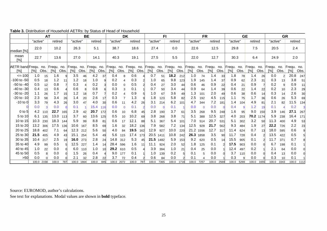
25

Table 3. Distribution of Household AETRs: by Status of Head of Household AT BE DK FI FR GE GR

"active" retired "active" retired "active" retired "active" retired "active" retired "active" retired "active" retired

median [%] 22.0 10.2 26.3 5.1 38.7 18.6 27.4 0.0 22.6 12.5 29.8 7.5 20.5 2.4

mean [%]

22.7 13.6 27.0 14.1 40.3 19.1 27.5 5.5 22.0 12.7 30.3 6.4 24.9 2.0

AETR band [%]

Frequ. [%]

no. Obs.

Frequ. [%]

no. Obs.

Frequ. [%]

no. Obs.

Frequ. [%]

no. Obs.

Frequ. [%]

no. Obs.

Frequ. [%]

no. Obs.

Frequ. [%]

no. Obs.

Frequ. [%]

no. Obs.

Frequ. [%]

no. Obs.

Frequ. [%]

no. Obs.

Frequ. [%]

no. Obs.

Frequ. [%]

no. Obs.

Frequ. [%]

no. Obs.

Frequ. [%]

no. Obs.

<=-100 1.0 15 1.6 9 3.5 46 4.2 37 0.4 8 0.6 4 0.7 51 18.2 212 1.0 74 1.4 33 1.8 78 1.4 26 0.0 2 20.8 247 -100 to -50 0.5 18 1.2 11 1.2 18 1.0 9 0.2 4 0.3 2 1.0 65 9.8 123 1.9 145 1.4 37 0.9 62 2.3 31 0.3 13 3.8 51 -50 to -40 0.5 12 0.8 7 0.3 4 0.2 3 0.0 0 0.5 2 0.4 27 3.0 44 0.6 46 0.9 22 0.4 21 0.9 7 0.2 9 0.9 11 -40 to -30 0.4 13 0.6 4 0.6 8 0.8 6 0.3 3 0.1 1 0.7 50 3.4 44 0.9 64 1.4 39 0.6 22 1.4 22 0.2 10 2.3 29 -30 to -20 1.1 26 1.7 15 1.2 18 0.7 7 0.2 4 0.9 5 1.0 67 3.6 49 1.3 101 2.0 49 0.6 38 0.6 14 0.3 14 2.6 30 -20 to -10 2.3 58 3.4 26 1.4 20 2.6 17 0.3 7 1.3 9 1.8 123 5.8 82 2.5 192 4.5 115 1.1 75 1.7 36 0.6 26 5.3 69

-10 to 0 3.3 79 4.3 26 3.0 47 4.0 30 0.6 11 4.2 26 3.1 214 6.2 101 4.7 344 7.2 181 1.4 104 4.9 81 2.1 82 11.5 134

0 0.0 3 0.0 0 0.1 1 15.4 116 0.0 0 0.1 2 0.0 0 0.1 1 0.0 0 0.0 0 0.4 9 1.2 19 0.1 4 0.2 3

0 to 5 4.2 110 22.7 165 2.9 42 20.7 172 0.6 10 6.8 45 2.8 190 3.7 61 3.5 268 9.5 248 1.6 95 9.0 150 3.9 146 27.1 267

5 to 10 6.1 135 13.0 113 3.7 60 13.6 125 0.5 10 10.2 69 3.8 268 3.8 71 5.1 388 12.5 327 4.0 203 70.2 1174 5.9 238 16.4 171

10 to 15 10.3 230 18.3 144 5.9 99 8.8 81 0.6 17 12.1 88 5.1 367 5.4 101 7.0 514 20.7 531 5.1 302 3.2 50 11.3 400 4.9 53

15 to 20 13.2 306 17.5 136 10.6 167 8.5 69 1.6 32 18.2 136 7.9 582 7.2 134 12.5 928 21.7 562 9.3 484 1.9 27 22.2 726 2.2 23

20 to 25 18.8 402 7.1 64 12.3 212 5.6 50 4.0 84 19.5 162 12.9 927 10.0 220 21.2 1556 12.7 317 11.4 624 0.7 13 18.0 595 0.6 9

25 to 30 21.5 405 4.9 43 15.1 254 5.4 49 5.6 115 17.4 173 20.5 1411 10.8 242 26.3 1858 3.5 90 11.7 728 0.4 2 13.5 422 0.5 5

30 to 35 10.4 217 2.5 19 16.0 273 2.8 24 14.8 312 5.3 45 21.5 1482 5.9 153 9.2 620 0.5 14 15.5 905 0.1 2 11.7 371 0.7 8

35 to 40 4.9 99 0.5 5 12.5 227 1.4 14 28.4 596 1.6 11 11.1 924 2.0 52 1.8 125 0.1 2 17.5 903 0.0 0 6.7 198 0.1 1

40 to 45 1.0 22 0.0 0 6.0 110 1.0 10 29.2 610 0.5 4 3.9 394 1.0 21 0.4 25 0.0 1 12.4 497 0.2 1 2.1 64 0.0 0 45 to 50 0.5 8 0.0 0 1.5 26 0.4 4 9.0 177 0.1 1 1.0 139 0.2 5 0.1 5 0.0 0 3.7 110 0.0 0 0.4 13 0.0 0

>50 0.0 0 0.0 0 2.1 32 2.8 22 3.7 72 0.4 2 0.6 84 0.0 2 0.1 4 0.0 1 0.3 9 0.0 0 0.3 10 0.1 1 100.0 2158 100.0 787 100.0 1664 100.0 845 100.0 2072 100.0 787 100.0 7365 100.0 1718 100.0 7257 100.0 2569 100.0 5269 100.0 1655 100.0 3343 100.0 1112


26

Table 3. (continued) IR IT LU NL PT SP UK

"active" retired "active" retired "active" retired "active" retired "active" retired "active" retired "active" retired

median [%] 15.0 0.0 24.8 10.0 15.7 9.1 27.3 14.0 15.9 0.0 16.3 0.0 20.8 4.9

mean [%]

17.6 4.7 27.4 12.8 19.5 15.5 28.6 19.4 20.9 4.6 19.5 8.5 20.3 -0.2

AETR band [%]

Frequ. [%]

no. Obs.

Frequ. [%]

no. Obs.

Frequ. [%]

no. Obs.

Frequ. [%]

no. Obs.

Frequ. [%]

no. Obs.

Frequ. [%]

no. Obs.

Frequ. [%]

no. Obs.

Frequ. [%]

no. Obs.

Frequ. [%]

no. Obs.

Frequ. [%]

no. Obs.

Frequ. [%]

no. Obs.

Frequ. [%]

no. Obs.

Frequ. [%]

no. Obs.

Frequ. [%]

no. Obs.

<=-100 1.6 36 1.2 8 0.1 7 2.1 51 0.2 4 0.4 3 2.7 66 1.5 14 1.8 62 0.3 7 0.0 1 0.1 1 3.1 134 7.9 119 -100 to -50 0.9 21 1.4 8 0.3 25 2.4 50 1.2 23 1.1 7 0.8 25 0.1 1 0.7 29 0.5 15 0.2 4 0.0 1 1.5 62 9.8 151 -50 to -40 0.7 19 2.0 13 0.5 12 0.7 27 0.9 18 0.5 3 0.3 10 0.0 0 0.5 17 0.3 5 0.1 2 0.1 1 0.5 20 3.3 52 -40 to -30 0.7 23 0.7 4 0.6 26 0.7 23 1.3 23 0.6 3 0.2 6 0.0 0 0.3 14 0.1 2 0.1 3 0.1 1 0.8 31 4.2 67 -30 to -20 1.4 40 0.4 3 0.4 29 1.2 29 2.3 44 0.7 3 0.3 10 0.0 0 0.6 21 0.7 10 0.1 5 0.2 2 0.7 30 3.7 59 -20 to -10 2.5 71 1.1 5 1.3 60 2.3 60 3.7 64 3.4 15 0.7 23 0.3 4 0.7 42 1.8 23 0.4 14 0.3 3 1.3 53 4.5 70

-10 to 0 5.8 169 2.4 15 2.4 134 7.7 208 7.2 131 3.4 17 1.3 42 3.7 34 2.3 86 5.0 43 1.6 53 1.8 31 2.9 114 6.1 98

0 1.5 42 65.9 317 0.0 0 2.1 46 0.0 0 0.0 0 0.1 3 0.1 1 0.0 0 59.1 767 0.0 0 47.5 573 0.1 3 0.0 0

0 to 5 7.5 249 6.4 33 2.2 127 16.8 367 6.5 110 19.1 93 0.8 25 4.3 40 5.2 192 18.9 199 4.3 171 12.3 155 2.2 89 10.6 169

5 to 10 10.5 348 4.2 24 3.2 161 13.6 364 10.6 191 29.3 153 1.8 55 12.8 130 11.5 418 6.2 51 13.1 496 15.8 202 3.7 154 19.7 322

10 to 15 17.0 526 7.7 30 6.2 315 16.0 445 14.0 285 19.0 103 3.2 105 34.5 376 20.0 726 4.3 36 23.3 817 12.5 164 8.4 352 17.8 288

15 to 20 18.9 553 3.7 21 12.0 643 22.9 585 15.0 302 9.6 51 7.4 253 20.1 200 24.8 838 1.4 28 25.9 928 6.9 91 20.0 847 9.7 156

20 to 25 12.4 327 1.4 8 22.3 1143 8.8 238 13.7 256 5.9 33 17.7 566 7.4 82 14.9 484 0.8 8 20.9 736 2.2 25 35.0 1382 2.4 39

25 to 30 9.6 222 0.9 7 24.7 1279 1.9 69 10.4 181 3.6 19 29.1 861 8.2 75 8.2 217 0.4 6 6.2 215 0.2 2 17.2 622 0.2 4

30 to 35 6.9 142 0.5 4 14.6 741 0.5 19 7.1 128 2.0 11 24.6 716 3.9 42 6.6 150 0.1 2 2.1 63 0.1 1 2.2 81 0.1 1

35 to 40 2.1 40 0.3 2 6.6 329 0.1 5 3.9 63 0.3 2 5.4 159 2.2 18 1.5 35 0.0 1 0.9 32 0.0 0 0.3 14 0.0 0

40 to 45 0.1 3 0.0 0 2.1 110 0.0 0 1.5 26 0.9 4 2.2 61 0.4 5 0.2 3 0.0 0 0.5 18 0.0 0 0.0 0 0.0 0 45 to 50 0.0 0 0.0 0 0.2 17 0.0 1 0.4 6 0.1 1 0.7 21 0.4 4 0.0 0 0.0 0 0.2 6 0.0 0 0.0 0 0.0 0

>50 0.0 0 0.0 0 0.4 17 0.0 0 0.0 0 0.0 0 0.4 14 0.2 2 0.1 5 0.0 0 0.0 2 0.0 0 0.0 1 0.0 0 100.0 2831 100.0 502 100.0 5175 100.0 2587 100.0 1855 100.0 521 100.0 3021 100.0 1028 100.0 3339 100.0 1203 100.0 3566 100.0 1253 100.0 3989 100.0 1595

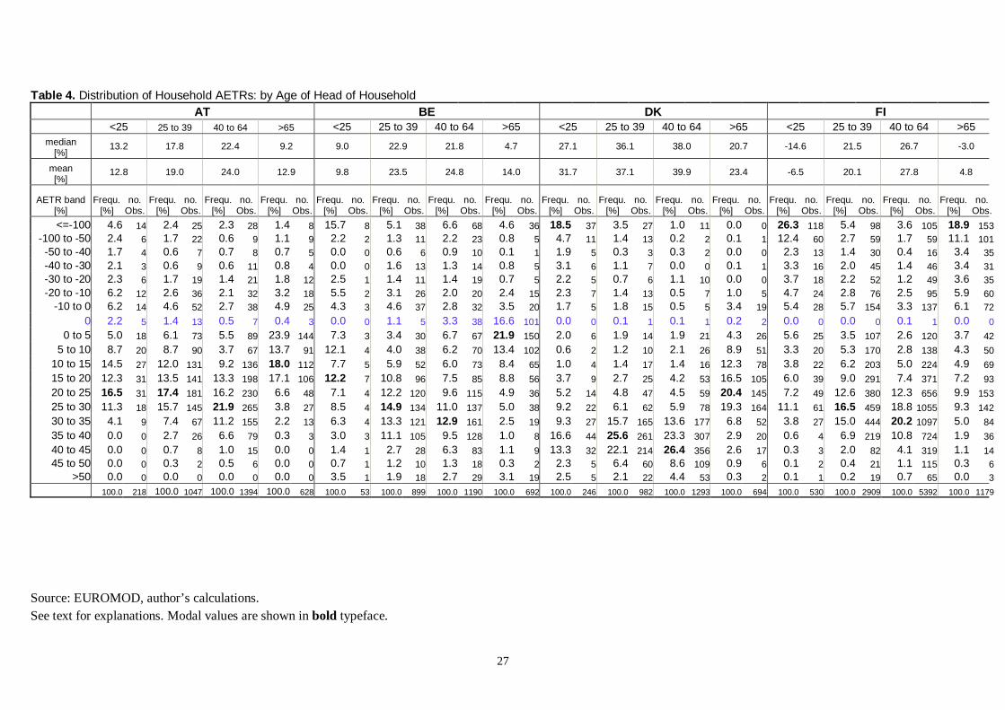
27

Table 4. Distribution of Household AETRs: by Age of Head of Household AT BE DK FI

<25 25 to 39 40 to 64 >65 <25 25 to 39 40 to 64 >65 <25 25 to 39 40 to 64 >65 <25 25 to 39 40 to 64 >65 median

[%] 13.2 17.8 22.4 9.2 9.0 22.9 21.8 4.7 27.1 36.1 38.0 20.7 -14.6 21.5 26.7 -3.0

mean [%]

12.8 19.0 24.0 12.9 9.8 23.5 24.8 14.0 31.7 37.1 39.9 23.4 -6.5 20.1 27.8 4.8

AETR band [%]

Frequ. [%]

no. Obs.

Frequ. [%]

no. Obs.

Frequ. [%]

no. Obs.

Frequ. [%]

no. Obs.

Frequ. [%]

no. Obs.

Frequ. [%]

no. Obs.

Frequ. [%]

no. Obs.

Frequ. [%]

no. Obs.

Frequ. [%]

no. Obs.

Frequ. [%]

no. Obs.

Frequ. [%]

no. Obs.

Frequ. [%]

no. Obs.

Frequ. [%]

no. Obs.

Frequ. [%]

no. Obs.

Frequ. [%]

no. Obs.

Frequ. [%]

no. Obs.

<=-100 4.6 14 2.4 25 2.3 28 1.4 8 15.7 8 5.1 38 6.6 68 4.6 36 18.5 37 3.5 27 1.0 11 0.0 0 26.3 118 5.4 98 3.6 105 18.9 153-100 to -50 2.4 6 1.7 22 0.6 9 1.1 9 2.2 2 1.3 11 2.2 23 0.8 5 4.7 11 1.4 13 0.2 2 0.1 1 12.4 60 2.7 59 1.7 59 11.1 101-50 to -40 1.7 4 0.6 7 0.7 8 0.7 5 0.0 0 0.6 6 0.9 10 0.1 1 1.9 5 0.3 3 0.3 2 0.0 0 2.3 13 1.4 30 0.4 16 3.4 35-40 to -30 2.1 3 0.6 9 0.6 11 0.8 4 0.0 0 1.6 13 1.3 14 0.8 5 3.1 6 1.1 7 0.0 0 0.1 1 3.3 16 2.0 45 1.4 46 3.4 31-30 to -20 2.3 6 1.7 19 1.4 21 1.8 12 2.5 1 1.4 11 1.4 19 0.7 5 2.2 5 0.7 6 1.1 10 0.0 0 3.7 18 2.2 52 1.2 49 3.6 35-20 to -10 6.2 12 2.6 36 2.1 32 3.2 18 5.5 2 3.1 26 2.0 20 2.4 15 2.3 7 1.4 13 0.5 7 1.0 5 4.7 24 2.8 76 2.5 95 5.9 60

-10 to 0 6.2 14 4.6 52 2.7 38 4.9 25 4.3 3 4.6 37 2.8 32 3.5 20 1.7 5 1.8 15 0.5 5 3.4 19 5.4 28 5.7 154 3.3 137 6.1 72

0 2.2 5 1.4 13 0.5 7 0.4 3 0.0 0 1.1 5 3.3 38 16.6 101 0.0 0 0.1 1 0.1 1 0.2 2 0.0 0 0.0 0 0.1 1 0.0 0

0 to 5 5.0 18 6.1 73 5.5 89 23.9 144 7.3 3 3.4 30 6.7 67 21.9 150 2.0 6 1.9 14 1.9 21 4.3 26 5.6 25 3.5 107 2.6 120 3.7 42

5 to 10 8.7 20 8.7 90 3.7 67 13.7 91 12.1 4 4.0 38 6.2 70 13.4 102 0.6 2 1.2 10 2.1 26 8.9 51 3.3 20 5.3 170 2.8 138 4.3 50

10 to 15 14.5 27 12.0 131 9.2 136 18.0 112 7.7 5 5.9 52 6.0 73 8.4 65 1.0 4 1.4 17 1.4 16 12.3 78 3.8 22 6.2 203 5.0 224 4.9 69

15 to 20 12.3 31 13.5 141 13.3 198 17.1 106 12.2 7 10.8 96 7.5 85 8.8 56 3.7 9 2.7 25 4.2 53 16.5 105 6.0 39 9.0 291 7.4 371 7.2 93

20 to 25 16.5 31 17.4 181 16.2 230 6.6 48 7.1 4 12.2 120 9.6 115 4.9 36 5.2 14 4.8 47 4.5 59 20.4 145 7.2 49 12.6 380 12.3 656 9.9 153

25 to 30 11.3 18 15.7 145 21.9 265 3.8 27 8.5 4 14.9 134 11.0 137 5.0 38 9.2 22 6.1 62 5.9 78 19.3 164 11.1 61 16.5 459 18.8 1055 9.3 142

30 to 35 4.1 9 7.4 67 11.2 155 2.2 13 6.3 4 13.3 121 12.9 161 2.5 19 9.3 27 15.7 165 13.6 177 6.8 52 3.8 27 15.0 444 20.2 1097 5.0 84

35 to 40 0.0 0 2.7 26 6.6 79 0.3 3 3.0 3 11.1 105 9.5 128 1.0 8 16.6 44 25.6 261 23.3 307 2.9 20 0.6 4 6.9 219 10.8 724 1.9 36

40 to 45 0.0 0 0.7 8 1.0 15 0.0 0 1.4 1 2.7 28 6.3 83 1.1 9 13.3 32 22.1 214 26.4 356 2.6 17 0.3 3 2.0 82 4.1 319 1.1 1445 to 50 0.0 0 0.3 2 0.5 6 0.0 0 0.7 1 1.2 10 1.3 18 0.3 2 2.3 5 6.4 60 8.6 109 0.9 6 0.1 2 0.4 21 1.1 115 0.3 6

>50 0.0 0 0.0 0 0.0 0 0.0 0 3.5 1 1.9 18 2.7 29 3.1 19 2.5 5 2.1 22 4.4 53 0.3 2 0.1 1 0.2 19 0.7 65 0.0 3

100.0 218 100.0 1047 100.0 1394 100.0 628 100.0 53 100.0 899 100.0 1190 100.0 692 100.0 246 100.0 982 100.0 1293 100.0 694 100.0 530 100.0 2909 100.0 5392 100.0 1179


28

Table 4. (continued) FR GE GR IR


[%] 1.8 19.6 21.3 11.2 5.9 27.2 24.0 7.5 0.8 19.5 18.6 -1.7 5.1 13.1 10.2 0.0

mean [%]

4.1 17.8 21.4 11.1 7.2 26.6 27.5 6.0 10.7 22.9 24.1 3.0 4.2 14.7 14.9 3.5

AETR band [%]

Frequ. [%]

no. Obs.

Frequ. [%]

no. Obs.

Frequ. [%]

no. Obs.

Frequ. [%]

no. Obs.

Frequ. [%]

no. Obs.

Frequ. [%]

no. Obs.

Frequ. [%]

no. Obs.

Frequ. [%]

no. Obs.

Frequ. [%]

no. Obs.

Frequ. [%]

no. Obs.

Frequ. [%]

no. Obs.

Frequ. [%]

no. Obs.

Frequ. [%]

no. Obs.

Frequ. [%]

no. Obs.

Frequ. [%]

no. Obs.

Frequ. [%]

no. Obs.

<=-100 10.0 57 3.9 127 3.2 150 2.3 55 22.6 68 8.6 187 6.4 131 1.5 20 2.4 4 0.7 7 1.7 33 18.9 250 11.4 15 7.7 57 6.3 76 1.1 10-100 to -50 6.1 36 3.1 109 2.6 126 2.9 74 8.4 26 2.1 67 1.5 46 1.8 17 2.1 3 0.3 5 0.6 15 3.6 54 3.3 10 0.8 10 2.0 30 1.8 15-50 to -40 2.3 11 0.9 31 0.8 38 1.4 35 4.7 8 0.5 14 0.2 13 1.0 6 0.4 1 0.2 3 0.2 7 0.8 11 1.7 5 1.1 14 0.6 12 1.3 14-40 to -30 3.5 21 1.2 39 1.2 57 1.5 39 4.3 9 0.8 18 0.8 19 1.2 15 0.0 0 0.3 3 0.4 11 2.7 37 2.4 7 0.7 11 1.7 22 0.5 3-30 to -20 7.9 44 1.7 62 1.6 71 2.4 60 2.6 9 1.3 42 0.5 18 0.6 10 0.5 1 0.6 7 0.5 16 2.4 31 3.2 11 3.3 35 2.7 41 0.5 3-20 to -10 8.7 48 3.1 109 3.0 140 5.3 130 1.0 5 2.4 70 1.6 62 1.6 27 0.7 1 1.1 15 1.4 38 6.2 86 6.0 18 7.6 85 4.1 67 0.9 9

-10 to 0 10.4 55 6.0 204 4.4 212 8.7 214 2.6 12 2.7 91 2.4 80 4.6 60 14.7 28 3.4 50 5.1 119 16.1 202 9.0 30 7.3 82 7.6 131 1.3 16

0 0.2 1 0.0 0 0.0 0 0.0 0 1.5 6 0.3 11 2.3 49 1.4 16 24.7 45 2.1 37 2.0 53 0.9 12 3.7 8 1.9 17 9.0 108 70.4 468

0 to 5 3.4 19 4.2 150 3.7 185 10.5 268 2.2 10 2.2 62 3.1 110 8.6 107 13.2 25 5.0 77 9.8 203 23.6 267 8.3 32 4.3 65 7.5 161 6.6 57

5 to 10 6.6 41 6.1 217 5.3 264 11.8 301 3.0 12 4.7 110 11.5 367 71.2 936 6.1 10 5.4 84 9.0 231 14.4 172 11.0 36 6.8 105 8.3 194 4.4 47

10 to 15 5.7 34 7.8 272 7.9 375 19.4 488 5.5 18 4.7 138 4.3 176 2.9 37 8.5 22 11.8 181 9.3 222 3.7 50 13.5 46 14.1 211 13.0 269 6.6 45

15 to 20 8.2 50 13.5 472 12.4 606 18.4 466 8.4 34 6.5 185 8.6 288 1.8 22 15.1 31 22.4 302 16.2 393 2.9 39 13.7 45 17.5 245 13.0 271 2.2 17

20 to 25 12.8 72 18.6 648 19.3 941 11.1 274 8.6 34 9.7 273 8.8 322 1.0 15 6.5 16 19.2 262 12.9 314 1.4 24 8.4 24 9.6 123 10.0 182 1.3 12

25 to 30 12.9 80 22.0 723 23.0 1094 3.5 88 8.5 31 8.3 292 10.4 418 0.5 3 2.9 7 11.4 164 11.7 251 0.8 11 2.7 5 9.4 107 6.8 111 0.5 7

30 to 35 1.5 9 6.6 201 9.1 418 0.6 15 6.3 28 13.9 388 11.9 497 0.1 2 1.8 4 10.6 140 9.5 220 1.1 18 1.6 2 6.5 73 5.1 69 0.2 2

35 to 40 0.0 0 1.2 38 1.9 89 0.1 2 7.2 28 16.1 425 13.0 456 0.2 2 0.5 1 4.6 58 6.4 136 0.4 6 0.0 0 1.5 14 2.0 25 0.3 3

40 to 45 0.0 0 0.2 3 0.5 22 0.0 1 2.2 9 11.7 253 9.4 238 0.0 0 0.0 0 0.8 10 2.4 53 0.0 1 0.0 0 0.0 0 0.2 3 0.0 045 to 50 0.0 0 0.0 1 0.1 4 0.0 0 0.0 0 3.4 58 2.9 52 0.0 0 0.0 0 0.3 6 0.4 7 0.0 0 0.0 0 0.0 0 0.0 0 0.0 0

>50 0.0 0 0.0 0 0.2 5 0.0 0 0.4 1 0.0 1 0.4 7 0.0 0 0.0 0 0.0 1 0.4 10 0.0 0 0.0 0 0.0 0 0.0 0 0.0 0

100.0 578 100.0 3406 100.0 4797 100.0 2510 100.0 348 100.0 2685 100.0 3349 100.0 1295 100.0 199 100.0 1412 100.0 2332 100.0 1271 100.0 294 100.0 1254 100.0 1772 100.0 728

29

Table 4. (continued) IT LU NL PT


[%] 19.6 23.4 23.4 10.0 11.8 14.8 13.5 9.2 -56.3 26.7 27.2 13.2 12.1 15.1 15.8 0.0

mean [%]

20.9 25.7 26.6 14.3 11.6 16.6 20.0 15.6 3.0 26.3 28.7 17.1 12.9 19.2 21.3 8.1

AETR band [%]

Frequ. [%]

no. Obs.

Frequ. [%]

no. Obs.

Frequ. [%]

no. Obs.

Frequ. [%]

no. Obs.

Frequ. [%]

no. Obs.

Frequ. [%]

no. Obs.

Frequ. [%]

no. Obs.

Frequ. [%]

no. Obs.

Frequ. [%]

no. Obs.

Frequ. [%]

no. Obs.

Frequ. [%]

no. Obs.

Frequ. [%]

no. Obs.

Frequ. [%]

no. Obs.

Frequ. [%]

no. Obs.

Frequ. [%]

no. Obs.

Frequ. [%]

no. Obs.

<=-100 0.3 1 0.5 8 0.4 18 2.3 44 0.0 0 0.7 6 2.4 22 0.4 2 38.1 95 6.0 95 6.2 104 0.0 0 2.6 4 2.5 36 2.9 74 0.3 9-100 to -50 0.5 2 0.8 21 0.8 23 2.7 44 0.8 1 2.1 21 1.6 18 0.5 2 13.2 36 0.6 13 0.4 6 0.2 2 0.2 1 0.4 10 1.1 24 0.8 15-50 to -40 1.3 1 1.0 11 0.3 13 0.7 22 0.6 1 1.7 16 0.3 4 0.4 2 2.7 7 0.4 8 0.2 4 0.0 0 0.3 3 0.6 8 0.4 10 0.3 5-40 to -30 0.1 1 0.7 16 0.8 27 0.6 13 0.5 1 2.0 16 1.0 10 0.2 1 1.0 4 0.1 3 0.1 2 0.0 0 0.3 1 0.3 5 0.5 13 0.2 3-30 to -20 0.4 2 0.8 20 0.6 26 1.2 20 2.3 4 2.8 27 1.7 17 0.6 2 1.7 7 0.2 4 0.2 4 0.0 0 0.3 4 0.5 10 0.9 12 0.4 10-20 to -10 1.1 3 1.6 35 1.9 68 1.9 34 3.5 6 4.9 42 2.6 25 3.3 10 2.7 7 0.8 11 0.8 15 0.5 5 1.5 2 0.9 18 1.1 36 1.4 22

-10 to 0 1.0 6 2.4 57 3.8 141 7.3 155 3.4 5 8.5 82 6.2 58 3.3 14 2.4 8 1.4 21 1.2 24 5.0 39 3.0 7 2.8 36 3.9 70 4.4 42

0 0.2 1 0.4 9 1.0 28 1.7 32 0.0 0 0.0 0 0.0 0 0.0 0 1.3 4 0.1 2 0.3 5 0.0 0 0.0 0 0.1 4 4.6 91 53.1 733

0 to 5 3.7 14 2.1 60 4.6 164 17.5 284 8.6 11 6.0 55 8.7 76 19.5 80 0.9 3 0.7 13 1.3 21 4.9 41 10.7 29 5.9 75 5.4 116 17.5 197

5 to 10 6.4 18 3.7 80 4.7 168 13.9 290 14.6 18 9.5 89 14.1 148 30.0 128 2.3 7 1.6 23 1.7 32 15.3 142 19.7 60 13.4 166 8.7 191 6.5 69

10 to 15 7.7 22 7.5 147 7.8 303 15.7 331 33.4 46 12.8 147 14.9 150 18.3 80 3.5 11 2.6 47 3.6 68 39.5 389 31.1 74 20.4 261 16.4 379 6.1 71

15 to 20 32.9 75 14.4 315 11.8 468 22.1 435 19.1 30 14.0 157 13.1 130 10.4 45 1.4 3 8.3 135 7.3 144 22.5 198 20.6 53 25.1 300 21.6 459 4.5 69

20 to 25 26.5 68 21.7 476 18.9 710 8.5 170 8.9 10 13.7 139 11.3 112 6.3 30 9.5 29 19.5 301 13.8 290 5.7 55 8.6 16 13.4 168 14.5 282 2.3 28

25 to 30 13.7 34 21.4 430 21.9 854 2.1 57 3.8 3 10.6 99 9.3 87 2.9 13 13.0 36 29.2 423 27.7 506 3.3 30 0.5 2 7.2 73 8.5 136 1.1 16

30 to 35 3.0 12 13.3 269 12.2 460 1.0 23 0.0 0 6.9 66 6.3 62 2.3 11 3.8 13 22.8 330 24.5 435 0.9 9 0.5 1 5.3 41 7.5 103 0.8 9

35 to 40 0.3 1 5.1 104 6.1 220 0.4 10 0.0 0 2.4 22 4.4 40 0.6 3 1.5 4 3.7 53 6.6 123 1.3 6 0.0 0 1.2 9 1.5 25 0.2 2

40 to 45 0.2 1 1.7 37 1.9 70 0.2 4 0.5 1 1.1 11 1.7 15 0.7 3 0.0 0 1.3 14 2.5 46 0.7 8 0.0 0 0.0 1 0.3 2 0.0 045 to 50 0.0 0 0.1 6 0.3 12 0.1 1 0.0 0 0.2 2 0.4 4 0.1 1 0.6 1 0.3 4 1.1 21 0.1 1 0.0 0 0.0 0 0.0 0 0.0 0

>50 1.0 1 0.8 15 0.4 14 0.0 0 0.0 0 0.0 0 0.0 0 0.0 0 0.3 1 0.3 6 0.6 10 0.1 1 0.0 0 0.0 0 0.1 3 0.2 2

100.0 263 100.0 2116 100.0 3787 100.0 1969 100.0 137 100.0 997 100.0 978 100.0 427 100.0 276 100.0 1506 100.0 1860 100.0 926 100.0 257 100.0 1221 100.0 2026 100.0 1302

30


<25 25 to 39 40 to 64 >65 <25 25 to 39 40 to 64 >65 median

[%] 8.3 14.6 14.5 0.0 1.6 19.4 17.8 4.7

mean [%]

12.6 17.0 18.9 8.4 -2.9 13.8 16.3 0.4

AETR band [%]

Frequ. [%]

no. Obs.

Frequ. [%]

no. Obs.

Frequ. [%]

no. Obs.

Frequ. [%]

no. Obs.

Frequ. [%]

no. Obs.

Frequ. [%]

no. Obs.

Frequ. [%]

no. Obs.

Frequ. [%]

no. Obs.

<=-100 0.9 1 0.5 11 0.4 16 0.4 4 31.3 125 19.2 413 12.9 337 7.6 116 -100 to -50 0.0 0 0.3 3 0.4 9 0.1 2 4.4 15 2.5 52 2.6 69 10.6 166 -50 to -40 0.0 0 0.2 2 0.0 0 0.0 1 1.6 6 0.5 10 1.1 29 3.1 50 -40 to -30 0.3 1 0.1 1 0.1 4 0.1 1 1.9 7 0.8 18 1.3 36 4.0 64 -30 to -20 0.4 1 0.4 5 0.3 11 0.2 3 2.0 7 0.8 16 1.1 26 4.1 67 -20 to -10 0.7 3 0.9 11 0.7 16 0.2 4 1.6 6 1.3 27 1.4 39 4.9 77

-10 to 0 1.9 3 4.3 62 2.8 83 2.2 46 4.4 15 3.0 65 2.6 69 6.2 101

0 7.9 8 0.9 13 6.9 173 55.7 876 1.5 5 0.1 1 0.1 3 0.0 0

0 to 5 17.2 20 6.5 126 8.0 206 10.3 170 2.9 10 1.3 30 3.8 100 10.6 173

5 to 10 27.3 38 15.6 259 12.9 367 13.3 229 2.2 8 2.6 55 5.4 150 19.6 328

10 to 15 15.6 20 23.3 390 20.0 519 9.2 160 6.4 25 6.0 138 8.6 237 17.6 294

15 to 20 12.6 16 23.4 393 20.7 571 5.6 98 11.7 47 14.2 330 18.9 522 9.0 149

20 to 25 9.8 11 16.8 284 17.8 472 2.1 38 20.1 78 28.7 596 27.1 726 2.0 34

25 to 30 4.9 4 4.8 71 5.3 144 0.5 11 7.7 24 17.2 308 11.0 290 0.5 9

30 to 35 0.5 1 1.3 18 1.9 44 0.2 2 0.0 0 1.7 33 1.8 46 0.2 4

35 to 40 0.0 0 0.2 3 1.0 28 0.0 1 0.0 0 0.2 4 0.3 10 0.0 0

40 to 45 0.0 0 0.3 6 0.5 12 0.1 2 0.0 0 0.0 0 0.0 0 0.0 0 45 to 50 0.0 0 0.1 2 0.2 4 0.0 0 0.0 0 0.0 0 0.0 0 0.0 0

>50 0.0 0 0.1 3 0.1 2 0.0 0 0.2 1 0.0 0 0.0 1 0.0 0

100.0 127 100.0 1663 100.0 2681 100.0 1648 100.0 379 100.0 2096 100.0 2690 100.0 1632

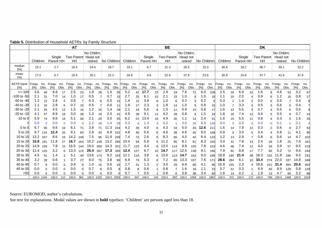
31

Table 5. Distribution of Household AETRs: by Family Structure AT BE DK

Children Single

Parent HH Two Parent

HH

No Chldrn; Head not

retired No Children Children Single


HH

No Chldrn; Head not



HH

No Chldrn; Head not

retired No Children median

[%] 15.1 2.7 16.4 24.4 18.7 19.1 -5.7 21.3 26.5 15.3 35.4 18.2 36.7 39.1 32.2

mean [%]

17.5 5.7 19.4 25.1 22.2 20.8 -3.6 22.9 27.9 23.5 35.9 15.8 37.7 41.6 37.9

AETR band [%]

Frequ. [%]

no. Obs.

Frequ. [%]

no. Obs.

Frequ. [%]

no. Obs.

Frequ. [%]

no. Obs.

Frequ. [%]

no. Obs.

Frequ. [%]

no. Obs.

Frequ. [%]

no. Obs.

Frequ. [%]

no. Obs.

Frequ. [%]

no. Obs.

Frequ. [%]

no. Obs.

Frequ. [%]

no. Obs.

Frequ. [%]

no. Obs.

Frequ. [%]

no. Obs.

Frequ. [%]

no. Obs.

Frequ. [%]

no. Obs.

<=-100 3.6 40 8.8 17 2.5 23 1.9 28 1.6 35 5.2 42 17.7 23 2.9 19 7.6 72 6.0 108 2.5 18 6.9 10 1.6 8 4.6 53 3.2 57-100 to -50 2.1 31 7.0 14 1.0 17 0.5 7 0.7 15 2.7 25 6.1 10 2.1 15 1.0 8 1.0 16 1.1 10 2.0 4 0.9 6 1.2 16 0.8 17-50 to -40 1.2 12 2.8 5 0.8 7 0.3 6 0.5 12 1.4 12 3.9 6 1.0 6 0.2 3 0.2 5 0.3 2 1.4 2 0.0 0 0.5 7 0.4 8-40 to -30 1.1 16 2.8 6 0.7 10 0.5 7 0.6 11 1.9 17 2.3 3 1.8 14 1.0 9 0.9 15 1.0 7 3.3 4 0.5 3 0.6 6 0.4 7-30 to -20 2.1 29 4.5 13 1.5 16 1.2 16 1.4 29 2.1 19 5.6 8 1.5 11 0.9 10 0.8 17 1.6 13 5.5 9 0.7 4 0.5 6 0.5 8-20 to -10 4.1 57 8.9 18 3.0 39 1.3 19 2.0 41 4.9 39 9.1 11 4.2 28 0.8 9 1.5 24 1.8 18 7.4 13 0.6 5 0.5 8 0.7 14

-10 to 0 5.9 74 9.6 18 5.1 56 2.1 29 3.0 55 6.2 51 13.4 16 4.9 35 1.1 14 2.4 41 1.6 15 5.5 11 0.8 4 0.3 5 1.6 29

0 0.0 0 0.0 0 0.0 0 2.2 28 1.4 28 0.3 4 1.3 3 0.2 1 3.0 26 8.9 140 0.0 0 0.0 0 0.0 0 0.1 2 0.1 4

0 to 5 6.7 90 9.6 19 6.1 71 3.8 71 11.3 234 4.2 39 4.0 6 4.3 33 5.0 40 12.6 211 1.6 14 7.8 12 0.3 2 0.6 9 2.7 53

5 to 10 9.7 116 12.4 33 9.1 83 2.9 43 6.9 152 4.8 46 5.6 8 4.6 38 4.6 45 9.0 168 0.9 9 3.0 5 0.4 4 0.8 11 4.1 80

10 to 15 13.2 167 8.6 19 14.2 148 7.5 95 11.9 239 7.4 72 2.6 6 8.3 66 4.0 42 6.4 123 1.2 13 2.9 7 0.8 6 0.6 14 4.7 102

15 to 20 15.8 191 11.8 27 16.7 164 10.2 149 13.2 285 10.4 94 5.9 9 11.2 85 8.1 81 8.3 150 3.4 31 7.8 13 2.4 18 1.8 25 7.6 161

20 to 25 14.9 159 7.8 15 16.5 144 19.0 268 14.3 331 11.7 122 4.4 8 13.0 114 9.9 105 7.8 153 4.6 46 7.4 12 4.0 34 3.9 57 9.5 219

25 to 30 11.4 125 3.2 6 13.3 119 25.4 287 17.3 330 13.4 127 6.7 10 14.7 117 12.5 138 9.1 186 7.9 82 8.8 17 7.7 65 5.2 72 9.6 244

30 to 35 4.5 51 1.4 2 5.1 49 13.6 174 9.2 193 12.1 119 3.8 6 13.6 113 14.7 162 9.0 186 18.8 190 21.4 38 18.3 152 11.8 186 9.5 231

35 to 40 3.2 28 0.6 1 3.7 27 6.0 75 3.8 80 6.9 73 5.3 8 7.2 65 13.3 157 7.6 171 28.6 284 6.1 10 33.4 274 22.0 337 14.8 348

40 to 45 0.7 8 0.0 0 0.9 8 1.0 15 0.6 15 2.7 31 1.3 2 3.0 29 6.9 80 4.1 90 15.9 155 2.3 4 18.8 151 31.4 460 20.6 46445 to 50 0.0 0 0.0 0 0.0 0 0.7 8 0.5 8 0.8 8 0.6 1 0.8 7 1.6 19 1.1 23 5.7 51 0.3 1 6.9 50 8.9 128 5.8 129

>50 0.0 0 0.0 0 0.0 0 0.0 0 0.0 0 0.7 7 0.5 1 0.8 6 3.8 38 3.4 60 1.6 14 0.2 1 1.9 13 4.7 66 3.2 68 100.0 1194 100.0 213 100.0 981 100.0 1325 100.0 2093 100.0 947 100.0 145 100.0 802 100.0 1058 100.0 1887 100.0 972 100.0 173 100.0 799 100.0 1468 100.0 2243

Source: EUROMOD, author’s calculations. See text for explanations. Modal values are shown in bold typeface. ‘Children’ are persons aged less than 18.

32

Table 5. (continued) FI FR GE

Children Single


HH

No Chldrn; Head not



HH

No Chldrn; Head not



HH

No Chldrn; Head not

retired No Children

median [%] 18.5 7.2 20.3 27.4 22.1 15.7 -9.8 17.0 22.3 17.6 21.5 -2.2 24.1 30.0 9.7

mean [%] 19.5 5.5 21.4 27.9 23.1 15.1 -13.2 17.0 22.1 19.6 21.2 0.1 24.4 31.0 24.7

AETR band [%]

Frequ. [%]

no. Obs.

Frequ. [%]

no. Obs.

Frequ. [%]

no. Obs.

Frequ. [%]

no. Obs.

Frequ. [%]

no. Obs.

Frequ. [%]

no. Obs.

Frequ. [%]

no. Obs.

Frequ. [%]

no. Obs.

Frequ. [%]

no. Obs.

Frequ. [%]

no. Obs.

Frequ. [%]

no. Obs.

Frequ. [%]

no. Obs.

Frequ. [%]

no. Obs.

Frequ. [%]

no. Obs.

Frequ. [%]

no. Obs.

<=-100 5.2 91 15.0 36 2.8 55 5.5 176 10.1 383 4.9 161 20.8 76 2.8 85 3.9 197 3.0 228 11.9 228 32.1 137 5.1 91 6.7 154 4.6 178-100 to -50 2.9 64 4.6 15 2.5 49 2.6 92 5.3 215 4.8 160 14.5 55 3.5 105 2.9 151 2.3 185 3.0 83 4.2 27 2.6 56 1.2 43 1.6 73-50 to -40 1.2 28 1.4 6 1.2 22 0.8 25 1.5 66 0.9 32 2.2 8 0.8 24 1.2 62 1.1 83 0.7 19 1.7 8 0.3 11 0.5 16 0.7 22-40 to -30 2.1 48 4.6 12 1.5 36 1.4 46 2.1 90 1.6 54 2.8 11 1.4 43 1.3 69 1.3 102 1.1 21 1.7 7 0.8 14 0.9 20 1.0 40-30 to -20 2.0 50 2.3 8 2.0 42 1.4 56 2.2 104 2.2 79 4.4 17 2.0 62 2.2 110 2.1 158 1.6 45 2.1 13 1.4 32 0.6 21 0.6 34-20 to -10 3.3 91 3.6 13 3.3 78 2.2 84 3.5 164 4.4 149 5.1 20 4.2 129 3.3 165 3.7 278 3.1 84 5.0 26 2.4 58 1.2 47 1.4 80

-10 to 0 5.2 154 6.7 25 4.8 129 3.6 140 4.5 237 7.4 251 9.5 35 7.2 216 5.0 254 5.7 434 3.2 97 3.9 24 3.0 73 1.7 66 3.0 146

0 0.0 0 0.0 0 0.0 0 0.0 0 0.0 1 0.0 0 0.0 0 0.0 0 0.0 1 0.0 1 0.0 0 0.0 0 0.0 0 2.4 63 1.9 82

0 to 5 5.1 133 7.5 19 4.5 114 2.3 101 2.8 161 5.6 191 5.0 18 5.6 173 3.4 185 5.5 431 2.3 74 1.9 10 2.4 64 2.0 67 4.8 215

5 to 10 6.8 190 8.3 34 6.5 156 2.5 118 3.0 188 7.8 269 8.9 33 7.6 236 4.1 227 7.0 554 5.6 125 6.4 23 5.4 102 3.5 128 30.7 1300

10 to 15 8.2 249 7.9 27 8.3 222 3.8 168 4.4 269 9.1 312 6.4 24 9.5 288 6.3 329 11.2 857 5.5 169 3.9 23 6.0 146 4.0 151 3.6 200

15 to 20 11.4 361 8.5 34 12.1 327 6.2 300 6.6 433 14.7 505 9.1 34 15.4 471 9.7 530 13.8 1089 9.2 254 5.3 28 10.5 226 7.6 249 5.3 275

20 to 25 15.4 474 12.1 38 16.2 436 10.6 544 10.4 764 18.5 628 6.5 24 20.0 604 17.8 992 16.1 1307 12.1 324 5.6 28 14.2 296 8.6 308 5.4 320

25 to 30 14.3 485 10.2 43 15.3 442 18.9 991 16.0 1232 13.7 464 3.1 11 15.1 453 26.5 1432 18.7 1521 12.1 363 8.4 35 13.3 328 9.1 379 5.6 381

30 to 35 9.6 354 4.7 20 10.7 334 21.6 1147 15.8 1298 3.6 122 0.5 2 4.0 120 9.9 507 6.7 521 16.4 416 9.7 38 18.6 378 11.6 498 6.9 499

35 to 40 4.7 206 1.9 12 5.4 194 11.2 725 7.8 777 0.8 25 0.9 3 0.7 22 1.9 102 1.3 104 9.3 250 4.8 24 10.9 226 18.2 661 10.8 661

40 to 45 1.6 76 0.2 2 1.9 74 4.0 321 2.9 342 0.2 6 0.3 1 0.2 5 0.4 19 0.3 20 2.0 50 2.5 9 1.8 41 15.3 449 9.2 45045 to 50 0.8 37 0.3 2 0.9 35 0.9 102 0.6 107 0.0 0 0.0 0 0.0 0 0.1 5 0.1 5 0.7 5 0.7 2 0.7 3 4.5 105 2.7 105

>50 0.4 21 0.2 2 0.4 19 0.6 65 0.4 67 0.0 0 0.0 0 0.0 0 0.1 4 0.1 5 0.3 3 0.0 0 0.4 3 0.3 6 0.2 6 100.0 3112 100.0 348 100.0 2764 100.0 5201 100.0 6898 100.0 3408 100.0 372 100.0 3036 100.0 5341 100.0 7883 100.0 2610 100.0 462 100.0 2148 100.0 3431 100.0 5067

33

Table 5. (continued) GR IR IT

Children Single


HH

No Chldrn; Head not



HH

No Chldrn; Head not



HH

No Chldrn; Head not

retired No Children

median [%] 20.5 9.3 21.0 16.2 7.2 8.1 -13.6 11.2 10.7 3.4 23.8 16.0 24.2 24.5 18.1

mean [%] 25.3 15.1 25.7 21.8 18.3 10.6 -16.2 13.8 17.5 16.2 26.2 19.0 26.6 27.4 23.2

AETR band [%]

Frequ. [%]

no. Obs.

Frequ. [%]

no. Obs.

Frequ. [%]

no. Obs.

Frequ. [%]

no. Obs.

Frequ. [%]

no. Obs.

Frequ. [%]

no. Obs.

Frequ. [%]

no. Obs.

Frequ. [%]

no. Obs.

Frequ. [%]

no. Obs.

Frequ. [%]

no. Obs.

Frequ. [%]

no. Obs.

Frequ. [%]

no. Obs.

Frequ. [%]

no. Obs.

Frequ. [%]

no. Obs.

Frequ. [%]

no. Obs.

<=-100 1.7 23 10.0 9 1.1 14 1.2 27 7.8 271 9.0 107 32.5 58 3.6 49 4.4 46 3.5 51 0.5 12 1.5 2 0.4 10 0.2 10 1.1 59-100 to -50 0.4 7 0.0 0 0.4 7 0.7 19 1.7 70 1.7 32 3.4 13 1.3 19 2.0 27 1.6 33 1.2 34 0.2 1 1.3 33 0.2 8 1.3 56-50 to -40 0.1 3 0.5 1 0.1 2 0.2 8 0.5 19 1.2 26 2.0 6 1.0 20 0.5 9 0.8 19 1.2 20 1.4 1 1.1 19 0.1 2 0.4 27-40 to -30 0.4 7 3.6 4 0.1 3 0.7 16 1.2 44 1.7 31 1.9 10 1.7 21 0.8 10 0.7 12 1.4 34 0.8 3 1.4 31 0.2 6 0.4 23-30 to -20 0.6 8 2.7 2 0.4 6 0.6 18 1.2 47 4.3 71 4.2 14 4.4 57 1.1 16 0.9 19 1.1 35 1.9 5 1.1 30 0.2 8 0.6 33-20 to -10 1.5 21 9.0 6 1.0 15 1.9 51 3.0 119 9.3 154 12.4 34 8.6 120 0.9 24 0.8 25 2.5 63 6.3 5 2.2 58 0.8 22 1.5 77

-10 to 0 5.2 82 12.1 11 4.7 71 7.7 184 9.0 317 12.8 227 18.3 47 11.6 180 1.0 30 0.9 32 4.3 114 8.5 16 3.9 98 1.5 53 4.2 245

0 0.1 1 0.0 0 0.1 1 5.0 143 3.4 146 0.0 0 0.0 0 0.0 0 24.4 284 35.4 601 0.5 15 1.1 3 0.5 12 0.4 11 1.2 55

0 to 5 4.6 70 9.8 9 4.2 61 9.6 240 15.4 502 5.4 129 5.4 22 5.4 107 7.3 154 7.1 186 3.5 100 10.6 17 2.9 83 2.0 68 8.9 422

5 to 10 4.3 74 2.9 3 4.4 71 8.9 255 11.4 423 9.0 208 8.6 35 9.1 173 6.1 150 5.7 174 4.1 106 7.2 19 3.8 87 3.1 95 8.2 450

10 to 15 9.4 137 8.0 7 9.5 130 9.9 291 8.0 338 14.9 329 6.2 29 17.0 300 10.2 212 9.7 242 7.8 204 7.7 23 7.9 181 5.6 161 10.6 599

15 to 20 20.0 269 17.6 13 20.2 256 16.8 474 12.0 496 13.4 289 4.0 19 15.6 270 13.6 269 11.2 289 9.4 276 16.4 35 8.8 241 14.7 441 18.8 1017

20 to 25 15.6 210 13.6 11 15.8 199 14.0 399 9.6 406 7.9 162 0.9 5 9.6 157 10.0 172 7.9 179 17.5 463 14.0 26 17.8 437 24.5 726 17.2 961

25 to 30 13.4 191 7.9 7 13.8 184 9.3 237 6.4 242 5.2 105 0.3 2 6.3 103 8.6 118 6.7 125 22.1 593 14.7 38 22.8 555 24.2 715 13.7 782

30 to 35 12.4 166 1.4 2 13.2 164 7.6 209 5.3 216 2.8 56 0.0 0 3.5 56 7.1 86 5.5 90 14.4 370 4.1 13 15.3 357 12.8 377 7.0 394

35 to 40 7.9 106 0.9 1 8.4 105 3.8 94 2.6 95 1.1 22 0.0 0 1.3 22 2.0 18 1.6 20 5.5 151 2.0 4 5.8 147 6.7 179 3.6 184

40 to 45 1.8 22 0.0 0 1.9 22 1.6 42 1.1 42 0.1 1 0.0 0 0.1 1 0.1 2 0.1 2 1.8 47 0.2 1 1.9 46 2.2 65 1.2 6545 to 50 0.4 5 0.0 0 0.4 5 0.2 8 0.2 8 0.0 0 0.0 0 0.0 0 0.0 0 0.0 0 0.3 11 0.0 0 0.3 11 0.2 7 0.1 8

>50 0.3 4 0.0 0 0.3 4 0.2 7 0.1 7 0.0 0 0.0 0 0.0 0 0.0 0 0.0 0 0.8 20 1.5 2 0.7 18 0.4 10 0.2 10 100.0 1406 100.0 86 100.0 1320 100.0 2722 100.0 3808 100.0 1949 100.0 294 100.0 1655 100.0 1627 100.0 2099 100.0 2668 100.0 214 100.0 2454 100.0 2964 100.0 5467

34

Table 5. (continued) LU NL PT

Children Single


HH

No Chldrn; Head not



HH

No Chldrn; Head not



HH

No Chldrn; Head not

retired No Children

median [%] 5.3 -5.1 6.0 19.1 15.1 23.3 -145.5 24.0 28.1 24.4 15.0 4.9 15.5 16.0 9.9

mean [%] 9.2 -2.9 10.2 24.6 22.4 24.6 -38.4 26.4 28.3 26.1 19.1 9.3 20.2 21.4 18.4

AETR band [%]

Frequ. [%]

no. Obs.

Frequ. [%]

no. Obs.

Frequ. [%]

no. Obs.

Frequ. [%]

no. Obs.

Frequ. [%]

no. Obs.

Frequ. [%]

no. Obs.

Frequ. [%]

no. Obs.

Frequ. [%]

no. Obs.

Frequ. [%]

no. Obs.

Frequ. [%]

no. Obs.

Frequ. [%]

no. Obs.

Frequ. [%]

no. Obs.

Frequ. [%]

no. Obs.

Frequ. [%]

no. Obs.

Frequ. [%]

no. Obs.

<=-100 2.1 15 6.0 5 1.6 10 1.3 14 0.9 15 6.4 95 49.9 71 1.4 24 9.8 185 7.1 199 3.5 86 6.8 19 2.9 67 1.8 33 1.2 37-100 to -50 3.4 32 9.2 10 2.7 22 0.5 6 0.6 10 0.4 6 2.4 4 0.1 2 2.4 51 1.6 51 0.6 19 1.6 5 0.4 14 1.1 17 0.9 31-50 to -40 2.3 21 5.6 5 1.9 16 0.0 0 0.1 2 0.3 4 2.2 3 0.1 1 0.6 15 0.4 15 0.5 14 0.2 3 0.5 11 0.6 8 0.5 12-40 to -30 2.7 22 4.5 4 2.5 18 0.3 3 0.4 6 0.1 2 1.2 2 0.0 0 0.2 7 0.2 7 0.5 11 1.8 4 0.3 7 0.4 10 0.3 11-30 to -20 4.4 40 4.2 5 4.4 35 0.6 7 0.7 10 0.2 4 1.2 2 0.1 2 0.4 11 0.2 11 0.8 19 0.9 3 0.8 16 0.4 8 0.5 17-20 to -10 7.6 64 10.5 10 7.2 54 1.0 9 1.7 19 1.0 16 4.2 6 0.7 10 1.0 19 0.8 22 1.3 40 3.0 11 1.0 29 0.9 20 1.1 38

-10 to 0 14.2 124 16.8 16 13.9 108 2.1 19 2.5 35 1.9 31 7.9 10 1.3 21 1.5 27 2.2 61 5.9 91 19.7 26 3.6 65 1.7 35 2.2 64

0 0.0 0 0.0 0 0.0 0 0.0 0 0.0 0 0.0 0 0.0 0 0.0 0 0.4 10 0.3 11 0.0 0 0.0 0 0.0 0 3.2 61 24.4 828

0 to 5 12.7 101 11.8 13 12.8 88 3.1 29 9.1 121 0.9 16 0.6 1 1.0 15 1.2 22 2.2 62 5.7 131 15.9 39 4.1 92 5.6 94 10.6 286

5 to 10 15.9 135 9.4 11 16.8 124 8.5 98 16.3 248 2.4 35 6.8 8 1.9 27 1.8 39 5.5 169 12.6 236 15.3 39 12.1 197 9.5 199 8.3 250

10 to 15 11.4 93 7.6 10 11.9 83 16.7 229 17.7 330 4.7 72 6.1 10 4.5 62 3.0 67 13.4 443 18.6 369 9.0 40 20.1 329 19.4 381 13.9 416

15 to 20 8.2 61 3.7 3 8.8 58 18.5 251 15.3 301 13.6 213 7.0 9 14.3 204 4.0 68 9.3 267 22.2 365 14.1 28 23.5 337 24.6 489 16.1 516

20 to 25 6.7 50 8.1 7 6.5 43 16.8 208 12.8 241 27.2 408 7.3 9 29.5 399 8.8 185 8.4 267 13.8 219 6.2 11 15.1 208 13.9 267 9.1 275

25 to 30 5.2 36 0.0 0 5.9 36 12.7 147 9.4 166 24.7 356 1.4 2 27.4 354 27.2 564 20.9 639 7.0 92 2.8 6 7.6 86 8.2 129 5.3 135

30 to 35 2.6 19 2.5 2 2.6 17 9.3 109 6.6 120 11.2 171 0.5 1 12.4 170 27.9 574 20.0 616 6.2 74 2.0 4 6.8 70 6.4 78 4.1 80

35 to 40 0.5 4 0.0 0 0.6 4 5.7 59 3.7 61 2.3 36 0.6 1 2.4 35 6.3 132 5.0 150 1.0 14 0.7 3 1.0 11 1.7 21 1.1 22

40 to 45 0.0 0 0.0 0 0.0 0 2.3 26 1.8 30 1.6 23 0.0 0 1.8 23 2.1 40 1.5 45 0.0 0 0.0 0 0.0 0 0.3 3 0.2 345 to 50 0.0 0 0.0 0 0.0 0 0.6 6 0.4 7 0.5 7 0.7 1 0.4 6 0.8 17 0.6 20 0.0 0 0.0 0 0.0 0 0.0 0 0.0 0

>50 0.0 0 0.0 0 0.0 0 0.0 0 0.0 0 0.5 7 0.0 0 0.6 7 0.4 9 0.3 11 0.0 0 0.0 0 0.0 0 0.3 5 0.2 5 100.0 817 100.0 101 100.0 716 100.0 1220 100.0 1722 100.0 1502 100.0 140 100.0 1362 100.0 2042 100.0 3066 100.0 1780 100.0 241 100.0 1539 100.0 1858 100.0 3026

35


Children Single


HH

No Chldrn; Head not



HH

No Chldrn; Head not

retired No Children

median [%] 14.2 3.8 14.6 12.8 9.6 14.1 -791.7 17.8 19.6 13.8

mean [%] 18.3 8.4 18.7 17.5 15.7 7.2 -97.0 14.8 17.5 14.7

AETR band [%]

Frequ. [%]

no. Obs.

Frequ. [%]

no. Obs.

Frequ. [%]

no. Obs.

Frequ. [%]

no. Obs.

Frequ. [%]

no. Obs.

Frequ. [%]

no. Obs.

Frequ. [%]

no. Obs.

Frequ. [%]

no. Obs.

Frequ. [%]

no. Obs.

Frequ. [%]

no. Obs.

<=-100 0.8 21 4.2 8 0.6 13 0.3 10 0.3 11 27.0 528 67.4 314 13.8 214 11.9 349 10.6 463-100 to -50 0.4 6 0.5 1 0.4 5 0.4 7 0.3 8 3.0 56 5.7 26 2.0 30 3.0 96 5.0 246-50 to -40 0.2 2 1.2 1 0.1 1 0.0 0 0.0 1 0.8 16 1.6 7 0.6 9 0.9 27 1.6 79-40 to -30 0.3 5 0.2 1 0.3 4 0.0 1 0.0 2 1.0 20 1.3 6 0.9 14 1.2 40 2.1 105-30 to -20 0.7 14 2.1 3 0.7 11 0.1 5 0.1 6 0.9 18 1.3 6 0.8 12 1.3 40 2.0 98-20 to -10 1.4 24 1.4 2 1.4 22 0.3 7 0.3 10 1.6 32 2.3 10 1.4 22 1.4 47 2.4 117

-10 to 0 7.0 133 28.0 40 5.7 93 1.5 51 1.2 61 3.8 75 5.2 23 3.3 52 2.6 80 3.6 1750 0.2 4 0.0 0 0.2 4 17.6 497 26.8 1066 0.0 0 0.0 0 0.0 0 0.3 9 0.2 9

0 to 5 7.2 145 13.9 20 6.8 125 7.4 230 8.9 377 2.3 45 1.5 6 2.5 39 3.0 99 5.3 2685 to 10 15.4 284 16.7 20 15.4 264 12.2 412 13.3 609 2.9 57 1.9 9 3.2 48 4.6 162 9.2 484

10 to 15 19.6 351 10.8 15 20.2 336 19.0 580 17.1 738 8.1 160 5.0 22 9.2 138 7.1 246 10.3 53415 to 20 22.2 384 17.2 17 22.5 367 18.3 605 14.9 694 20.4 414 5.0 22 25.4 392 14.1 480 12.8 63420 to 25 17.2 300 2.8 5 18.1 295 15.1 481 11.2 505 21.2 431 1.3 6 27.8 425 29.5 964 21.4 100325 to 30 4.1 65 0.3 1 4.4 64 5.2 163 3.7 165 5.8 121 0.4 2 7.6 119 16.7 506 11.8 51030 to 35 1.8 26 0.0 0 2.0 26 1.3 38 1.0 39 0.9 18 0.0 0 1.2 18 2.0 64 1.4 6535 to 40 0.9 14 0.5 1 0.9 13 0.5 18 0.4 18 0.3 6 0.0 0 0.4 6 0.2 8 0.2 840 to 45 0.4 6 0.0 0 0.4 6 0.4 14 0.3 14 0.0 0 0.0 0 0.0 0 0.0 0 0.0 045 to 50 0.1 3 0.0 0 0.1 3 0.2 3 0.1 3 0.0 0 0.0 0 0.0 0 0.0 0 0.0 0

>50 0.0 0 0.0 0 0.0 0 0.2 5 0.1 5 0.0 0 0.0 0 0.0 0 0.1 2 0.0 2 100.0 1787 100.0 135 100.0 1652 100.0 3127 100.0 4332 100.0 1997 100.0 459 100.0 1538 100.0 3219 100.0 4800

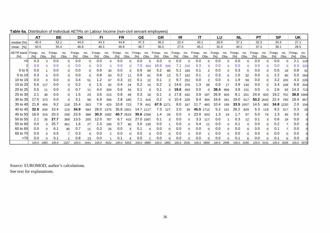
36

Table 6a. Distribution of Individual AETRs on Labour Income (non-civil servant employees)

AT BE DK FI FR GE GR IR IT LU NL PT SP UK median [%] 40.4 52.1 44.0 44.3 44.8 47.3 36.2 22.4 43.1 26.6 37.1 32.3 34.4 27.1

mean [%] 43.5 55.4 46.8 48.3 46.8 48.7 36.5 27.0 45.2 32.4 40.2 37.4 36.1 28.5

AETR band [%]

Frequ. [%]

no. Obs.

Frequ. [%]

no. Obs.

Frequ. [%]

no. Obs.

Frequ. [%]

no. Obs.

Frequ. [%]

no. Obs.

Frequ. [%]

no. Obs.

Frequ. [%]

no. Obs.

Frequ. [%]

no. Obs.

Frequ. [%]

no. Obs.

Frequ. [%]

no. Obs.

Frequ. [%]

no. Obs.

Frequ. [%]

no. Obs.

Frequ. [%]

no. Obs.

Frequ. [%]

no. Obs.

<0 0.3 3 0.0 0 0.0 0 0.0 0 0.0 0 0.0 0 0.0 0 0.0 0 0.0 0 0.0 0 0.0 0 0.0 0 0.0 0 2.1 119

0 0.0 0 0.0 0 0.0 0 0.0 0 0.0 0 7.0 494 16.9 339 7.1 226 0.3 9 0.0 0 0.0 0 0.0 0 0.0 0 6.3 333

0 to 5 0.0 1 0.0 0 0.0 0 0.9 30 0.0 3 0.9 84 5.2 88 5.1 160 0.1 2 0.0 0 0.3 5 0.0 0 0.5 19 0.8 41

5 to 10 0.3 5 0.0 0 0.0 0 0.8 50 0.2 11 0.9 61 0.8 12 5.7 162 0.1 2 0.3 6 1.0 32 0.0 0 2.2 90 5.0 264

10 to 15 0.0 0 0.0 0 3.4 51 1.2 67 0.3 22 0.1 12 0.1 2 9.7 252 0.0 2 0.0 0 1.9 59 0.0 0 3.2 105 4.3 226

15 to 20 5.6 117 0.0 0 0.2 5 1.5 92 0.4 24 0.2 14 0.2 3 14.6 376 1.3 59 0.9 17 3.9 130 0.0 0 3.4 108 6.8 334

20 to 25 0.5 11 0.0 0 0.7 11 4.4 330 0.6 34 0.1 9 0.1 3 19.6 493 0.0 0 38.4 806 3.9 131 0.0 0 2.6 93 14.3 713

25 to 30 2.1 36 0.0 0 1.5 23 3.6 215 0.8 49 0.3 16 0.1 3 17.8 432 3.9 187 26.9 603 8.1 251 24.9 920 19.2 702 38.8 1969

30 to 35 17.5 373 0.0 0 3.1 56 6.9 346 2.8 185 7.1 416 0.2 5 10.4 228 9.4 394 16.6 341 19.0 617 50.2 1642 22.4 790 19.4 957

35 to 40 21.8 456 9.2 118 15.4 263 7.9 425 10.8 723 7.9 641 67.5 1271 8.0 167 11.7 483 10.4 199 33.5 1057 14.5 383 34.8 1220 2.0 104

40 to 45 32.9 630 10.4 124 34.9 584 28.0 1375 35.8 2301 14.7 1117 7.3 127 2.0 39 45.5 1712 5.2 101 26.2 829 5.3 119 9.2 317 0.3 18

45 to 50 16.9 316 20.3 258 23.9 388 30.3 1582 40.7 2533 30.6 2289 1.4 26 0.0 0 23.9 920 1.3 24 1.7 57 5.0 74 1.3 45 0.0 0

50 to 55 2.1 35 27.7 368 13.5 205 12.0 787 6.7 415 27.0 1587 0.1 3 0.0 0 3.3 117 0.0 1 0.3 12 0.1 3 0.6 19 0.0 0

55 to 60 0.0 0 25.7 361 1.6 27 2.3 195 0.7 46 3.0 135 0.0 1 0.0 0 0.4 11 0.0 0 0.1 4 0.0 0 0.2 7 0.0 0

60 to 65 0.0 0 6.1 90 0.7 11 0.3 25 0.0 3 0.1 4 0.0 0 0.0 0 0.0 0 0.0 0 0.0 0 0.0 0 0.1 7 0.0 0

65 to 70 0.0 0 0.5 7 0.3 4 0.0 2 0.0 0 0.0 0 0.0 0 0.0 0 0.0 1 0.0 0 0.0 0 0.0 0 0.0 0 0.0 0

>70 0.0 0 0.1 1 0.8 13 0.0 1 0.1 4 0.0 1 0.0 0 0.0 0 0.0 0 0.0 0 0.1 6 0.0 0 0.1 6 0.0 0 100.0 1983 100.0 1327 100.0 1641 100.0 5522 100.0 6353 100.0 6880 100.0 1883 100.0 2535 100.0 3899 100.0 2098 100.0 3190 100.0 3141 100.0 3528 100.0 5078

Source: EUROMOD, author’s calculations. See text for explanations.

37

Table 6b. Comparison of Country Rankings (1998).

EUROMOD Martinez-Mongay

(2000) Rank mean AETR [%] mean AETR [%]

1 BE 55.4 BE 45.1

2 GE 48.7 FI 43.8

3 FI 48.3 GE 43.7

4 FR 46.8 DK 42.7

5 DK 46.8 FR 41.3

6 IT 45.2 AT 41.0

7 AT 43.5 NL 35.9

8 NL 40.2 IT 35.3

9 PT 37.4 LU 31.7

10 GR 36.5 SP 29.6

11 SP 36.1 GR 28.7

12 LU 32.4 UK 25.4

13 UK 28.5 PT 24.8

14 IR 27.0 IR 23.2

Source: EUROMOD, author’s calculations. See text for explanations. ‘Gross Earnings’ include employer SIC.

Table 7. Mean Individual AETRs (Labour Income) by Decile Group of Gross Earnings

% AT BE DK FI FR GE GR IR IT LU NL PT SP UK

Decile Group

1 28.3 42.3 50.5 20.3 42.6 6.4 6.3 6.5 32.3 22.7 30.2 29.2 27.0 -2.5 2 34.5 45.4 46.9 31.9 45.5 36.1 16.5 7.0 35.5 24.1 23.0 29.1 26.1 9.0 3 35.9 49.0 52.0 39.6 47.3 41.7 17.8 14.7 40.1 26.1 30.4 30.2 25.6 19.6 4 39.3 50.0 42.7 42.6 43.9 44.9 30.1 17.6 42.1 26.1 35.0 31.2 30.7 24.1 5 40.5 52.4 42.8 43.7 42.9 46.6 34.8 21.2 42.8 27.0 38.1 31.9 32.2 27.1 6 42.0 53.3 43.6 45.1 42.6 48.3 34.7 24.2 43.8 27.9 38.8 32.4 34.6 28.2 7 43.8 54.5 43.5 46.3 43.0 49.3 35.5 25.4 44.8 29.8 39.8 33.4 35.6 29.1 8 45.3 55.8 44.3 47.5 43.4 50.6 36.9 28.9 45.9 31.5 38.2 35.1 37.1 30.2 9 47.1 58.2 46.5 49.9 44.1 52.0 39.9 32.1 47.5 34.4 38.0 37.8 38.5 30.4

10 49.0 61.3 52.5 54.6 46.8 51.5 42.5 35.2 51.7 39.3 41.6 45.2 39.3 34.2

38

Table 8. Distribution of Marginal Effective Tax Rates

AT BE DK FI FR women men women men women men women men women men

median [%] 39.2% 42.8% total

49.9% 49.9% total

51.2% 51.2% total

45.3% 49.4% total

34.9% 34.9% total

METR band [%]

Frequ. [%]

no. Obs.

Frequ. [%]

no. Obs.

Frequ. [%]

no. Obs.

Frequ. [%]

no. Obs.

Frequ. [%]

no. Obs.

Frequ. [%]

no. Obs.

Frequ. [%]

no. Obs.

Frequ. [%]

no. Obs.

Frequ. [%]

no. Obs.

Frequ. [%]

no. Obs.

Frequ. [%]

no. Obs.

Frequ. [%]

no. Obs.

Frequ. [%]

no. Obs.

Frequ. [%]

no. Obs.

Frequ. [%]

no. Obs.

<0 0.0 1 0.0 0 0.0 1 1.2 17 2.3 28 1.8 45 0.8 16 1.2 23 1.0 39 0.0 3 0.0 6 0.0 9 0.6 34 0.6 38 0.6 72

0 17.0 297 9.4 251 12.5 548 8.5 89 7.9 106 8.2 195 1.5 18 1.1 15 1.2 33 8.1 987 12.5 1469 10.4 2456 4.1 240 2.4 179 3.2 419

0 to 5 0.1 2 0.1 4 0.1 6 0.0 0 0.0 0 0.0 0 0.0 0 0.1 1 0.0 1 1.3 206 2.2 378 1.7 584 0.5 31 0.5 36 0.5 67

5 to 10 0.0 0 0.0 0 0.0 0 0.0 0 0.1 2 0.1 2 0.5 9 0.4 8 0.4 17 0.8 72 0.8 92 0.8 164 0.6 33 1.0 66 0.8 99

10 to 15 1.6 26 0.3 5 0.8 31 3.9 49 2.2 35 3.0 84 0.1 2 0.1 1 0.1 3 0.5 55 0.3 44 0.4 99 0.7 43 1.3 95 1.1 138

15 to 20 17.2 242 2.9 58 8.8 300 0.1 1 0.3 5 0.2 6 0.1 1 0.0 0 0.0 1 0.5 43 0.3 38 0.4 81 1.6 89 2.2 153 1.9 242

20 to 25 1.2 25 0.6 21 0.8 46 0.5 7 1.1 14 0.8 21 0.1 1 0.1 1 0.1 2 2.5 181 1.7 104 2.1 285 7.9 447 8.7 608 8.3 1055

25 to 30 1.7 26 0.6 13 1.0 39 1.4 17 1.3 15 1.3 32 0.1 1 0.1 1 0.1 2 4.6 283 3.2 155 3.9 438 13.1 753 15.1 1059 14.2 1812

30 to 35 2.6 37 1.3 37 1.8 74 2.0 25 1.8 31 1.9 56 0.0 0 0.1 1 0.0 1 3.8 239 2.5 160 3.1 399 35.4 1987 30.9 2141 32.9 4128

35 to 40 13.2 188 13.8 327 13.6 515 5.3 65 4.1 59 4.6 124 0.0 0 0.0 0 0.0 0 5.4 350 3.4 238 4.3 588 16.0 880 17.9 1226 17.0 2106

40 to 45 19.3 276 31.2 687 26.3 963 9.0 113 6.3 93 7.5 206 0.0 0 0.0 0 0.0 0 18.4 1174 11.9 723 15.1 1897 7.6 411 6.8 449 7.2 860

45 to 50 14.7 229 23.0 519 19.6 748 28.1 387 27.2 436 27.6 823 11.1 203 10.4 200 10.7 403 22.1 1401 18.5 1186 20.3 2587 5.7 300 5.4 355 5.6 655

50 to 55 5.7 85 9.2 210 7.8 295 33.3 459 36.3 604 35.0 1063 58.8 1011 44.5 859 51.2 1870 17.2 1178 20.6 1421 18.9 2599 1.2 65 1.6 105 1.4 170

55 to 60 1.8 26 4.8 93 3.6 119 2.6 31 5.2 87 4.0 118 2.2 38 1.7 30 1.9 68 7.6 584 14.7 1269 11.2 1853 0.6 34 0.9 63 0.8 97

60 to 65 0.4 6 0.4 11 0.4 17 0.4 7 0.9 17 0.7 24 20.3 354 36.9 692 29.1 1046 1.3 96 2.9 277 2.1 373 0.4 22 0.7 51 0.6 73

65 to 70 0.1 2 0.1 5 0.1 7 0.1 1 0.0 0 0.0 1 1.2 16 0.5 10 0.8 26 0.4 16 0.5 18 0.4 34 0.2 9 0.3 25 0.3 34

70 to 75 0.1 1 0.1 3 0.1 4 0.2 2 0.0 1 0.1 3 0.6 8 0.2 5 0.4 13 0.4 19 0.3 20 0.4 39 0.3 15 0.4 24 0.3 39

75 to 80 0.0 0 0.0 1 0.0 1 0.0 0 0.0 0 0.0 0 0.4 6 0.3 5 0.4 11 0.4 15 0.3 15 0.3 30 0.2 11 0.4 26 0.3 37

80 to 85 0.0 1 0.0 0 0.0 1 0.0 0 0.0 0 0.0 0 1.2 21 1.6 25 1.4 46 0.5 21 0.1 9 0.3 30 0.2 7 0.2 16 0.2 23

85 to 90 0.0 0 0.0 0 0.0 0 0.0 0 0.0 0 0.0 0 0.1 1 0.0 0 0.0 1 0.2 8 0.2 9 0.2 17 0.2 13 0.2 18 0.2 31

90 to 95 0.0 0 0.0 0 0.0 0 0.1 1 0.0 0 0.0 1 0.0 0 0.0 0 0.0 0 0.1 8 0.0 2 0.1 10 0.8 45 0.6 42 0.7 87

95 to 100 1.9 22 1.8 48 1.8 70 3.1 37 2.5 33 2.8 70 0.9 16 0.6 10 0.8 26 3.8 156 3.0 128 3.4 284 1.6 89 1.3 88 1.4 177

>100 1.3 23 0.3 10 0.7 33 0.3 4 0.4 6 0.3 10 0.3 5 0.1 2 0.2 7 0.1 4 0.2 7 0.1 11 0.5 30 0.6 35 0.6 65 100.0 1515 100.0 2303 100.0 3818 100.0 1312 100.0 1572 100.0 2884 100.0 1727 100.0 1889 100.0 3616 100.0 7099 100.0 7768 100.0 14867 100.0 5588 100.0 6898 100.0 12486


39

Table 8. (continued)

GE GR IR IT LU women men women men women men women men women men

median [%] 53.2% 51.4% total

23.1% 30.0% total

30.8% 30.8% total

0.3 0.4 total

34.4% 35.9% total

METR band [%]

Frequ. [%]

no. Obs.

Frequ. [%]

no. Obs.

Frequ. [%]

no. Obs.

Frequ. [%]

no. Obs.

Frequ. [%]

no. Obs.

Frequ. [%]

no. Obs.

Frequ. [%]

no. Obs.

Frequ. [%]

no. Obs.

Frequ. [%]

no. Obs.

Frequ. [%]

no. Obs.

Frequ. [%]

no. Obs.

Frequ. [%]

no. Obs.

Frequ. [%]

no. Obs.

Frequ. [%]

no. Obs.

Frequ. [%]

no. Obs.

<0 0.2 7 0.2 9 0.2 16 1.2 20 1.3 45 1.3 65 0.0 0 0.0 0 0.0 0 0.0 1 0.0 2 0.0 3 0.0 0 0.1 2 0.1 2

0 5.2 237 3.8 187 4.4 424 33.7 628 22.2 844 25.9 1472 22.0 486 8.6 318 13.4 804 18.7 585 12.7 657 15.0 1242 9.1 111 5.4 121 6.8 232

0 to 5 1.0 36 0.2 8 0.5 44 3.9 59 2.0 79 2.6 138 1.3 20 6.8 231 4.8 251 0.5 9 0.7 31 0.6 40 0.0 0 0.0 0 0.0 0

5 to 10 0.1 3 0.0 0 0.0 3 0.7 13 1.0 39 0.9 52 0.1 2 1.2 60 0.8 62 3.3 109 2.7 150 2.9 259 0.4 5 0.8 11 0.7 16

10 to 15 1.2 48 0.3 18 0.7 66 2.6 39 7.0 243 5.5 282 0.5 13 3.1 161 2.1 174 0.2 6 0.4 22 0.3 28 17.1 207 16.9 313 17.0 520

15 to 20 0.6 42 0.1 6 0.3 48 6.8 117 5.3 193 5.8 310 1.9 30 5.1 194 3.9 224 1.6 53 0.4 20 0.9 73 5.5 56 4.5 82 4.9 138

20 to 25 3.0 126 1.2 77 2.0 203 9.0 138 4.7 155 6.1 293 6.6 116 6.2 219 6.4 335 2.2 74 1.9 102 2.0 176 4.6 47 2.6 43 3.3 90

25 to 30 1.3 69 1.9 85 1.6 154 7.2 109 15.0 521 12.5 630 10.5 160 12.0 344 11.5 504 7.0 244 1.9 103 3.9 347 6.3 78 5.5 111 5.8 189

30 to 35 5.5 183 6.5 345 6.0 528 7.6 122 7.7 254 7.7 376 9.3 153 15.9 441 13.5 594 22.6 685 16.4 850 18.7 1535 8.6 102 12.6 233 11.1 335

35 to 40 4.2 166 6.8 285 5.7 451 16.8 265 20.3 634 19.2 899 1.7 32 0.9 29 1.2 61 20.6 694 24.2 1324 22.8 2018 7.6 94 12.6 230 10.7 324

40 to 45 5.2 215 7.6 350 6.6 565 3.1 42 4.9 151 4.3 193 1.9 36 2.6 84 2.4 120 5.5 167 7.5 411 6.8 578 8.6 93 11.7 194 10.5 287

45 to 50 8.9 385 14.5 729 12.0 1114 4.4 63 5.6 170 5.2 233 19.2 294 23.7 657 22.0 951 12.0 356 19.0 949 16.4 1305 14.3 136 16.5 258 15.6 394

50 to 55 31.4 1328 32.3 1753 31.9 3081 0.5 10 1.0 34 0.9 44 17.8 261 9.7 212 12.6 473 2.5 69 6.6 339 5.1 408 13.9 138 8.3 144 10.4 282

55 to 60 20.6 749 16.3 773 18.2 1522 1.3 20 0.6 19 0.8 39 2.3 35 0.8 19 1.3 54 0.7 13 0.5 30 0.6 43 1.4 13 0.8 15 1.1 28

60 to 65 2.2 86 2.3 100 2.2 186 0.1 1 0.0 1 0.0 2 0.4 8 1.3 44 1.0 52 0.6 18 0.5 29 0.5 47 0.0 0 0.0 0 0.0 0

65 to 70 2.4 82 1.6 85 1.9 167 0.2 2 0.0 1 0.1 3 0.3 6 0.1 2 0.1 8 0.3 11 0.3 19 0.3 30 0.0 0 0.0 0 0.0 0

70 to 75 0.3 19 0.6 35 0.5 54 0.1 2 0.0 0 0.0 2 0.4 5 0.0 1 0.2 6 0.2 3 0.7 21 0.5 24 0.0 0 0.0 0 0.0 0

75 to 80 0.8 17 0.7 26 0.7 43 0.0 0 0.0 0 0.0 0 0.3 5 0.5 12 0.4 17 0.0 2 0.3 21 0.2 23 0.1 2 0.0 1 0.1 3

80 to 85 0.1 6 0.5 37 0.3 43 0.0 0 0.0 0 0.0 0 0.6 10 0.2 4 0.3 14 0.2 9 0.7 30 0.5 39 0.0 0 0.0 1 0.0 1

85 to 90 0.1 6 0.0 5 0.1 11 0.0 0 0.0 0 0.0 0 0.1 3 0.0 0 0.0 3 0.1 5 0.1 7 0.1 12 1.0 10 0.3 4 0.6 14

90 to 95 0.0 2 0.0 0 0.0 2 0.0 0 0.0 0 0.0 0 0.0 1 0.0 0 0.0 1 0.0 2 0.2 12 0.1 14 0.9 8 0.8 12 0.9 20

95 to 100 3.2 125 2.1 132 2.6 257 0.0 0 0.0 0 0.0 0 0.7 12 0.5 12 0.6 24 0.1 6 0.5 24 0.4 30 0.1 1 0.1 1 0.1 2

>100 2.7 102 0.7 33 1.6 135 0.9 14 1.4 43 1.2 57 2.0 31 0.8 24 1.3 55 0.8 24 1.8 90 1.4 114 0.6 5 0.4 8 0.5 13 100.0 4039 100.0 5078 100.0 9117 100.0 1664 100.0 3426 100.0 5090 100.0 1719 100.0 3068 100.0 4787 100.0 3145 100.0 5243 100.0 8388 100.0 1106 100.0 1784 100.0 2890

40


NL PT SP UK women men women men women men women men

median [%] 42.6% 42.6% total

26.0% 26.0% total

23.4% 24.8% total

31.4% 31.4% total

METR band [%]

Frequ. [%]

no. Obs.

Frequ. [%]

no. Obs.

Frequ. [%]

no. Obs.

Frequ. [%]

no. Obs.

Frequ. [%]

no. Obs.

Frequ. [%]

no. Obs.

Frequ. [%]

no. Obs.

Frequ. [%]

no. Obs.

Frequ. [%]

no. Obs.

Frequ. [%]

no. Obs.

Frequ. [%]

no. Obs.

Frequ. [%]

no. Obs.

<0 3.3 72 3.8 93 3.6 165 0.0 0 0.0 0 0.0 0 0.3 6 0.3 11 0.3 17 0.0 0 0.0 0 0.0 0

0 5.1 109 1.8 47 3.2 156 15.3 341 10.5 339 12.5 680 31.8 696 19.1 782 23.5 1478 11.5 351 5.0 149 8.0 500

0 to 5 0.0 2 0.0 1 0.0 3 0.0 0 0.1 3 0.0 3 2.0 45 1.1 50 1.4 95 0.0 1 0.0 0 0.0 1

5 to 10 0.0 0 0.0 1 0.0 1 0.2 3 0.4 17 0.3 20 7.1 156 5.4 224 6.0 380 3.1 94 0.1 3 1.5 97

10 to 15 0.0 1 0.0 1 0.0 2 13.4 306 14.1 494 13.8 800 0.1 3 0.4 23 0.3 26 0.2 5 0.0 0 0.1 5

15 to 20 0.0 1 0.1 2 0.1 3 6.2 184 2.4 71 4.0 255 3.1 69 4.7 188 4.2 257 2.6 79 1.5 48 2.0 127

20 to 25 0.0 1 0.0 1 0.0 2 4.3 87 7.5 261 6.2 348 10.1 220 19.7 847 16.4 1067 7.3 215 11.4 390 9.5 605

25 to 30 0.1 4 0.0 0 0.1 4 23.0 593 30.8 1169 27.5 1762 18.1 437 21.0 908 20.0 1345 16.4 496 12.0 400 14.0 896

30 to 35 20.4 482 2.1 49 10.0 531 1.5 31 4.8 108 3.4 139 22.9 482 19.4 782 20.7 1264 44.9 1318 50.3 1651 47.8 2969

35 to 40 15.7 321 16.3 454 16.1 775 19.6 408 14.9 443 16.9 851 1.6 36 2.9 121 2.5 157 4.6 136 13.5 475 9.5 611

40 to 45 30.2 645 27.2 734 28.5 1379 6.3 96 6.6 142 6.5 238 1.0 24 2.5 95 2.0 119 0.5 15 0.4 14 0.4 29

45 to 50 8.2 168 19.8 593 14.8 761 8.0 148 4.1 107 5.7 255 0.3 6 0.7 25 0.6 31 0.5 16 0.9 27 0.7 43

50 to 55 7.4 163 17.4 502 13.1 665 0.1 4 0.0 1 0.1 5 0.5 9 0.7 29 0.7 38 0.0 1 0.0 0 0.0 1

55 to 60 2.5 54 6.7 195 4.9 249 0.0 0 0.0 0 0.0 0 0.3 4 1.2 39 0.9 43 0.1 2 0.1 3 0.1 5

60 to 65 0.5 8 0.5 13 0.5 21 0.0 0 0.0 0 0.0 0 0.0 0 0.0 0 0.0 0 0.4 12 0.3 7 0.3 19

65 to 70 0.3 5 0.3 10 0.3 15 0.0 1 0.0 0 0.0 1 0.0 1 0.0 1 0.0 2 0.7 21 0.2 7 0.4 28

70 to 75 0.2 4 0.3 10 0.3 14 0.0 0 0.0 5 0.0 5 0.0 0 0.0 1 0.0 1 0.4 13 0.2 6 0.3 19

75 to 80 0.8 12 0.3 11 0.5 23 0.5 11 1.5 62 1.1 73 0.1 2 0.1 4 0.1 6 2.7 83 2.4 92 2.5 175

80 to 85 0.7 12 0.3 10 0.5 22 0.0 1 0.0 1 0.0 2 0.0 0 0.0 0 0.0 0 0.3 11 0.6 20 0.5 31

85 to 90 0.0 1 0.0 1 0.0 2 0.2 4 0.1 3 0.1 7 0.0 0 0.1 2 0.0 2 0.7 20 0.3 9 0.5 29

90 to 95 0.3 2 0.1 3 0.2 5 1.3 38 1.8 80 1.6 118 0.0 0 0.0 0 0.0 0 0.4 12 0.3 13 0.3 25

95 to 100 3.8 73 2.2 58 2.9 131 0.2 6 0.1 7 0.1 13 0.1 3 0.3 12 0.2 15 2.5 80 0.4 14 1.4 94

>100 0.4 9 0.4 10 0.4 19 0.0 1 0.2 11 0.1 12 0.7 12 0.1 8 0.3 20 0.3 9 0.1 4 0.2 13 100.0 2149 100.0 2799 100.0 4948 100.0 2263 100.0 3324 100.0 5587 100.0 2211 100.0 4152 100.0 6363 100.0 2990 100.0 3332 100.0 6322

41

Table 9a. Median METRs by Household Disposable Income, Women and Men

% AT BE DK FI FR GE GR IR IT LU NL PT SP UK Decile Group

w m w m w m w m w m w m w m w m w m w m w m w m w m w m

1 17.5 39.9 31.5 7.5 51.2 51.2 39.1 28.8 33.8 35.1 47.6 52.3 0.0 0.0 3.5 5.0 15.4 21.1 13.1 13.1 33.9 39.4 15.0 80.0 0.0 0.0 44.1 20.0 2 18.2 41.4 11.9 29.1 47.6 51.2 39.9 34.6 34.5 35.8 49.0 51.5 0.0 0.0 60.0 5.0 25.9 33.3 13.1 13.1 38.9 42.6 11.0 15.0 0.0 6.4 70.0 78.7 3 18.2 41.9 39.0 43.6 51.2 51.2 40.1 41.8 33.2 34.9 52.3 49.8 0.0 15.0 28.7 44.9 26.8 39.2 13.8 17.8 36.4 41.8 15.5 18.9 6.2 20.5 33.0 33.0 4 17.6 41.9 42.2 45.2 51.2 51.2 42.4 43.5 28.7 28.6 49.9 51.5 0.0 15.2 19.7 30.8 28.7 39.6 16.7 24.2 36.3 42.6 15.0 24.4 0.0 23.4 30.0 31.4 5 32.9 42.0 44.0 46.9 51.2 51.2 44.1 44.3 29.1 28.5 52.6 51.5 2.0 30.0 24.0 27.2 33.2 39.6 22.0 27.6 34.5 42.6 15.0 26.0 1.9 24.6 30.0 31.4 6 35.5 42.3 49.0 49.1 51.2 51.2 44.8 45.7 33.8 32.4 53.3 52.4 5.7 30.0 24.0 30.0 33.2 39.6 29.9 34.8 42.1 42.6 25.0 26.0 20.5 24.6 31.4 31.4 7 36.7 43.0 49.2 49.9 51.2 51.2 44.8 49.4 34.9 33.9 53.5 52.0 19.3 30.0 28.5 30.8 33.3 39.6 38.5 39.5 42.6 42.6 26.0 26.0 23.3 28.2 31.4 31.4 8 40.7 42.5 49.9 50.4 51.2 51.2 48.2 49.9 34.9 33.9 54.0 51.9 30.0 31.4 28.5 30.8 33.4 39.6 38.3 39.7 42.6 46.7 26.0 26.0 24.8 28.0 31.4 31.4 9 41.7 43.9 50.3 50.4 51.2 62.4 49.9 50.7 35.7 35.0 54.2 51.4 30.0 36.5 48.2 48.2 39.6 39.8 46.1 45.1 42.6 50.0 36.0 36.0 28.0 29.0 31.4 31.4

10 44.9 47.5 50.4 54.2 62.4 62.4 51.1 55.1 39.3 39.3 51.5 48.0 36.5 40.0 48.2 48.2 39.8 46.3 49.5 47.3 50.0 50.0 42.1 42.1 31.2 33.0 31.4 40.0

Table 9b. Median METRs by Earnings, Women and Men

% AT BE DK FI FR GE GR IR IT LU NL PT SP UK Decile Group

w m w m w m w m w m w m w m w m w m w m w m w m w m w m

1 1.0 28.3 37.4 11.8 51.2 51.2 39.3 41.1 31.8 32.5 29.0 46.2 0.0 0.0 24.0 5.0 21.2 21.6 13.1 22.8 33.9 42.6 15.0 15.5 0.0 6.4 10.0 28.1

2 17.7 33.1 42.8 39.0 51.2 51.2 35.8 42.2 33.7 32.7 52.6 50.7 0.0 0.0 28.5 15.2 26.1 23.5 21.5 23.4 33.9 43.9 15.5 15.0 1.9 1.9 30.0 30.0

3 29.1 40.9 46.0 45.1 51.2 51.2 35.8 36.8 34.1 34.9 51.2 47.8 12.8 0.0 28.5 25.5 33.3 33.3 27.5 22.9 36.4 38.5 26.0 24.9 0.2 6.4 30.3 31.4

4 39.4 40.7 49.1 45.4 51.2 51.2 41.3 41.6 34.9 34.9 53.3 51.2 23.3 19.3 30.8 29.9 33.2 33.2 32.5 24.9 42.6 42.6 26.0 25.0 24.6 20.0 33.0 33.0

5 40.0 42.7 50.4 49.9 51.2 51.2 44.8 44.3 34.9 34.9 52.9 51.9 31.1 15.0 30.8 30.8 33.2 33.2 36.4 25.5 42.6 42.6 26.0 26.0 27.9 24.1 31.4 33.0

6 40.0 41.4 49.9 49.9 51.2 51.2 45.0 44.8 34.9 34.9 53.6 52.4 31.4 29.2 49.2 30.8 39.6 39.6 41.7 29.0 42.6 42.6 26.0 26.0 23.3 23.3 31.4 31.4

7 41.9 42.0 50.4 49.9 51.2 51.2 49.9 49.5 34.9 34.9 54.2 53.0 38.2 31.0 49.2 30.8 39.6 39.6 47.0 34.4 40.0 39.4 36.0 26.0 28.0 26.6 31.4 31.4

8 42.0 42.2 50.0 49.9 57.5 51.2 50.2 50.1 34.9 32.5 54.7 54.1 37.7 30.0 49.2 30.8 39.6 39.6 50.4 36.5 50.0 41.4 36.0 26.0 28.0 28.0 31.4 31.4

9 47.1 47.6 50.4 50.4 62.4 62.4 50.7 50.7 35.7 33.9 56.8 51.7 36.5 36.5 48.3 48.3 40.2 42.4 50.6 43.3 49.6 50.0 37.0 36.0 31.7 29.2 26.1 23.5

10 46.8 47.8 54.2 54.6 62.4 62.4 55.6 55.6 42.8 39.3 53.2 46.0 40.0 45.0 48.3 48.3 45.7 47.8 47.2 45.3 50.0 50.0 42.2 42.2 37.6 39.0 40.0 40.0

Source: EUROMOD, author’s calculations. See text for explanations. ‘Earnings’ are gross but do not include employer SIC. Earnings decile groups are those for all people with earnings (men and women). Decile groups of household disposable income are based on equivalised household incomes (see footnote 15).

42

Table 10. Distribution of METRs by Poverty Status

AT BE DK FI FR GE GR poor non-poor poor non-poor poor non-poor poor non-poor poor non-poor poor non-poor poor non-poor

METR band [%]

Frequ. [%]

no. Obs.

Frequ. [%]

no. Obs.

Frequ. [%]

no. Obs.

Frequ. [%]

no. Obs.

Frequ. [%]

no. Obs.

Frequ. [%]

no. Obs.

Frequ. [%]

no. Obs.

Frequ. [%]

no. Obs.

Frequ. [%]

no. Obs.

Frequ. [%]

no. Obs.

Frequ. [%]

no. Obs.

Frequ. [%]

no. Obs.

Frequ. [%]

no. Obs.

Frequ. [%]

no. Obs.

<0 0.0 0 0.0 1 4.1 7 1.6 38 0.4 1 1.1 38 0.0 0 0.1 9 0.0 0 0.6 72 0.3 2 0.2 14 1.5 10 1.3 55

0 23.1 62 11.9 486 32.5 52 6.2 143 1.8 3 1.2 30 24.2 297 9.4 2159 5.9 60 3.0 359 20.5 50 3.8 374 61.8 403 21.3 1069

0 to 5 0.4 1 0.1 5 0.0 0 0.0 0 0.0 0 0.0 1 2.6 44 1.7 540 0.0 0 0.5 67 2.5 6 0.5 38 2.6 19 2.6 119

5 to 10 0.0 0 0.0 0 0.6 1 0.0 1 8.0 17 0.0 0 1.5 17 0.8 147 0.0 0 0.9 99 0.0 0 0.0 3 1.6 10 0.9 42

10 to 15 3.1 5 0.7 26 14.4 27 2.0 57 0.4 1 0.1 2 0.7 11 0.4 88 0.1 1 1.1 137 0.1 1 0.7 65 3.0 21 5.9 261

15 to 20 18.9 42 8.2 258 1.6 3 0.1 3 0.0 0 0.0 1 0.4 5 0.4 76 2.4 21 1.9 221 0.0 0 0.3 48 19.8 123 4.0 187

20 to 25 1.3 6 0.8 40 4.9 8 0.5 13 0.0 0 0.1 2 8.3 46 1.7 239 29.0 275 6.7 780 9.3 34 1.7 169 3.0 17 6.5 276

25 to 30 2.2 7 1.0 32 4.3 6 1.1 26 0.0 0 0.1 2 10.7 57 3.4 381 0.9 9 15.3 1803 2.3 7 1.6 147 3.6 21 13.6 609

30 to 35 2.0 3 1.8 71 4.5 11 1.7 45 0.0 0 0.0 1 6.1 33 2.9 366 12.5 116 34.6 4012 0.8 2 6.2 526 1.3 9 8.5 367

35 to 40 5.7 13 14.0 502 5.1 11 4.6 113 0.0 0 0.0 0 2.0 16 4.5 572 15.9 142 17.1 1964 3.1 9 5.8 442 1.4 8 21.4 891

40 to 45 10.7 22 27.2 941 3.0 4 7.9 202 0.0 0 0.0 0 2.6 25 15.9 1872 9.9 84 6.9 776 3.6 14 6.7 551 0.2 1 4.8 192

45 to 50 6.2 11 20.4 737 2.2 5 29.7 818 34.5 73 9.3 330 1.4 12 21.5 2575 4.5 38 5.6 617 7.0 13 12.2 1101 0.0 0 5.9 233

50 to 55 3.4 8 8.1 287 1.3 3 37.7 1060 36.9 72 52.1 1798 1.3 9 20.1 2590 2.8 23 1.3 147 3.3 9 32.9 3072 0.0 0 1.0 44

55 to 60 3.6 10 3.6 109 1.7 2 4.2 116 6.5 11 1.7 57 1.1 7 11.9 1846 0.8 8 0.8 89 0.5 4 18.8 1518 0.0 0 0.9 39

60 to 65 0.7 2 0.4 15 0.0 0 0.8 24 4.2 14 30.6 1032 1.5 9 2.2 364 1.1 8 0.6 65 3.3 6 2.2 180 0.0 0 0.0 2

65 to 70 0.5 3 0.1 4 0.0 0 0.0 1 0.7 1 0.8 25 0.7 6 0.4 28 1.4 13 0.2 21 18.6 38 1.3 129 0.0 0 0.1 3

70 to 75 0.3 1 0.1 3 0.0 0 0.1 3 0.0 0 0.4 13 1.2 9 0.3 30 0.1 1 0.3 38 0.5 3 0.5 51 0.0 0 0.0 2

75 to 80 0.4 1 0.0 0 0.0 0 0.0 0 0.0 0 0.4 11 1.2 5 0.3 25 0.1 1 0.3 36 2.9 2 0.7 41 0.0 0 0.0 0

80 to 85 0.0 0 0.0 1 0.0 0 0.0 0 0.0 0 1.5 46 1.4 9 0.2 21 0.0 0 0.2 23 0.0 0 0.3 43 0.0 0 0.0 0

85 to 90 0.0 0 0.0 0 0.0 0 0.0 0 0.0 0 0.0 1 1.5 6 0.1 11 0.2 2 0.2 29 0.0 0 0.1 11 0.0 0 0.0 0

90 to 95 0.0 0 0.0 0 0.0 0 0.0 1 0.0 0 0.0 0 0.8 6 0.0 4 0.0 0 0.7 87 0.0 0 0.0 2 0.0 0 0.0 0

95 to 100 15.8 27 1.0 43 19.5 35 1.4 35 6.0 11 0.4 15 27.9 162 1.8 122 10.5 96 0.7 81 16.2 60 2.1 197 0.0 0 0.0 0

>100 1.7 3 0.7 30 0.4 1 0.3 9 0.7 2 0.1 5 0.8 4 0.1 7 1.7 14 0.5 51 5.1 13 1.5 122 0.2 2 1.3 55 100.0 227 100.00 3591 100.0 176 100.00 2708 100.0 206 100.00 3410 100.0 795 100.00 14072 100.0 912 100.00 11574 100.0 273 100.00 8844 100.0 644 100.00 4446

Source: EUROMOD, author’s calculations. See text for explanations. Modal values are shown in bold typeface. ‘Poor’ persons are those living in households with per-capita income of less than 60% of median equivalised household disposable income.

43


IR IT LU NL PT SP UK poor non-poor poor non-poor poor non-poor poor non-poor poor non-poor poor non-poor poor non-poor

METR band [%]

Frequ. [%]

no. Obs.

Frequ. [%]

no. Obs.

Frequ. [%]

no. Obs.

Frequ. [%]

no. Obs.

Frequ. [%]

no. Obs.

Frequ. [%]

no. Obs.

Frequ. [%]

no. Obs.

Frequ. [%]

no. Obs.

Frequ. [%]

no. Obs.

Frequ. [%]

no. Obs.

Frequ. [%]

no. Obs.

Frequ. [%]

no. Obs.

Frequ. [%]

no. Obs.

Frequ. [%]

no. Obs.

<0 0.0 0 0.0 0 0.1 1 0.0 2 0.0 0 0.1 2 17.6 41 2.8 124 0.0 0 0.0 0 1.7 9 0.2 8 0.0 0 0.0 0

0 20.2 24 13.3 780 9.8 92 15.6 1150 4.7 13 7.0 219 10.1 27 2.9 129 22.1 176 11.3 504 53.4 350 20.3 1128 19.2 65 7.3 435

0 to 5 38.2 41 3.9 210 4.4 24 0.2 16 0.0 0 0.0 0 0.0 0 0.0 3 0.2 1 0.0 2 7.4 50 0.7 45 0.0 0 0.0 1

5 to 10 3.3 5 0.7 57 18.3 165 1.1 94 0.1 1 0.7 15 0.2 1 0.0 0 0.5 5 0.3 15 22.2 145 4.2 235 1.4 5 1.5 92

10 to 15 0.0 0 2.2 174 1.9 15 0.1 13 66.5 168 12.6 352 0.0 0 0.0 2 33.0 252 11.4 548 0.4 2 0.3 24 0.0 0 0.1 5

15 to 20 0.0 0 4.0 224 2.9 20 0.6 53 1.6 3 5.1 135 0.0 0 0.1 3 3.5 43 4.1 212 5.3 36 4.0 221 7.5 27 1.7 100

20 to 25 1.0 1 6.5 334 9.0 84 1.2 92 4.3 10 3.2 80 0.0 0 0.0 2 0.6 9 6.9 339 6.3 40 17.5 1027 0.2 1 10.0 604

25 to 30 0.6 1 11.8 503 8.7 87 3.3 260 2.4 7 6.1 182 0.3 1 0.0 3 13.3 124 29.4 1638 0.0 0 22.2 1345 7.0 26 14.4 870

30 to 35 0.0 0 13.9 594 23.4 217 18.2 1318 2.1 6 11.9 329 11.0 28 9.9 503 0.5 5 3.8 134 0.2 4 22.9 1260 6.4 23 50.2 2946

35 to 40 2.5 2 1.2 59 3.7 40 25.1 1978 0.7 3 11.6 321 20.3 44 15.8 731 0.1 3 19.0 848 0.2 1 2.7 156 1.2 4 9.9 607

40 to 45 0.8 1 2.4 119 6.1 59 6.8 519 0.0 0 11.4 287 16.1 51 29.2 1328 0.0 0 7.3 238 0.0 0 2.2 119 1.9 7 0.4 22

45 to 50 1.7 2 22.6 949 2.8 32 18.0 1273 0.8 1 16.9 393 0.0 0 15.6 761 0.0 0 6.4 255 0.0 0 0.6 31 0.6 2 0.7 41

50 to 55 0.0 0 13.0 473 1.1 6 5.5 402 0.0 0 11.4 282 0.0 0 13.8 665 0.0 0 0.1 5 0.0 0 0.7 38 0.2 1 0.0 0

55 to 60 22.7 21 0.8 33 0.5 4 0.6 39 0.3 1 1.1 27 0.0 0 5.2 249 0.0 0 0.0 0 0.2 1 1.0 42 0.0 0 0.1 5

60 to 65 3.8 4 0.9 48 0.6 4 0.5 43 0.0 0 0.0 0 1.2 3 0.4 18 0.0 0 0.0 0 0.0 0 0.0 0 1.0 4 0.3 15

65 to 70 0.0 0 0.1 8 0.1 3 0.3 27 0.0 0 0.0 0 0.8 3 0.3 12 0.0 1 0.0 0 0.2 2 0.0 0 3.8 13 0.2 15

70 to 75 0.0 0 0.2 6 1.5 8 0.3 16 0.0 0 0.0 0 0.9 3 0.2 11 0.2 3 0.0 2 0.1 1 0.0 0 2.5 9 0.2 10

75 to 80 0.0 0 0.4 17 0.0 0 0.2 23 0.3 1 0.0 2 1.2 5 0.5 18 9.8 73 0.0 0 0.5 3 0.1 3 22.2 90 1.4 85

80 to 85 3.2 3 0.2 11 0.5 3 0.5 36 0.0 0 0.0 1 0.6 3 0.5 19 0.2 2 0.0 0 0.0 0 0.0 0 3.7 14 0.3 17

85 to 90 0.0 0 0.0 3 0.2 1 0.1 11 5.2 11 0.1 3 0.0 0 0.0 2 0.9 7 0.0 0 0.0 0 0.0 2 3.8 11 0.3 18

90 to 95 0.0 0 0.0 1 0.4 6 0.1 8 9.1 16 0.2 4 0.0 0 0.2 5 12.8 116 0.2 2 0.0 0 0.0 0 1.9 8 0.2 17

95 to 100 2.0 3 0.5 21 0.5 5 0.4 25 0.6 1 0.0 1 17.0 47 2.1 84 1.1 13 0.0 0 1.3 7 0.1 8 14.2 53 0.6 41

>100 0.0 0 1.3 55 3.5 22 1.2 92 1.3 2 0.4 11 2.7 6 0.3 13 1.2 12 0.0 0 0.6 6 0.3 14 1.0 3 0.2 10 100.0 108 100.00 4679 100.0 898 100.00 7490 100.0 244 100.00 2646 100.0 263 100.00 4685 100.0 845 100.00 4742 100.0 657 100.00 5706 100.0 366 100.00 5956

44

Figure 1. AT: Household AETRs decomposed by income component

-100%

-80%

-60%

-40%

-20%

0%

20%

40%

60%

80%

100%

<=-1

00-1

00 to

-50

-50

to -4

0-4

0 to

-30

-30

to -2

0-2

0 to

-10

-10

to 0 0

0 to

5

5 to

10

10 to

15

15 to

20

20 to

25

25 to

30

30 to

35

35 to

40

40 to

45

45 to

50

>50

AETR band [%]

Co

ntr

ibu

tio

n t

o n

et t

axes

in e

ach

AE

TR

ban

d.

0%

50%

100%

150%

200%

250%

300%

350%

400%

450%

500%

'tax

bas

e' (

per

-cap

ita

pre

-tax

-ben

efit

inco

me)

re

lati

ve t

o m

edia

n

Other Benefits

Family Benefits

Housing Benefits

Social Assistance / Minimum Income

BE: Household AETRs decomposed by income component

-100%

-80%

-60%

-40%

-20%

0%

20%

40%

60%

80%

100%

<=-1

00-1

00 to

-50

-50

to -4

0-4

0 to

-30

-30

to -2

0-2

0 to

-10

-10

to 0 0

0 to

5

5 to

10

10 to

15

15 to

20

20 to

25

25 to

30

30 to

35

35 to

40

40 to

45

45 to

50

>50

AETR band [%]

Co

ntr

ibu

tio

n t

o n

et t

axes

in e

ach

AE

TR

ban

d.

0%

50%

100%

150%

200%

250%

300%

350%

400%

450%

500%

'tax

bas

e' (

per

-cap

ita

pre

-tax

-ben

efit

inco

me)

re

lati

ve t

o m

edia

n

DK: Household AETRs decomposed by income component

-100%

-80%

-60%

-40%

-20%

0%

20%

40%

60%

80%

100%

<=-1

00-1

00 to

-50

-50

to -4

0-4

0 to

-30

-30

to -2

0-2

0 to

-10

-10

to 0 0

0 to

5

5 to

10

10 to

15

15 to

20

20 to

25

25 to

30

30 to

35

35 to

40

40 to

45

45 to

50

>50

AETR band [%]

Co

ntr

ibu

tio

n t

o n

et t

axes

in e

ach

AE

TR

ban

d.

0%

50%

100%

150%

200%

250%

300%

350%

400%

450%

500%

'tax

bas

e' (

per

-cap

ita

pre

-tax

-ben

efit

inco

me)

re

lati

ve t

o m

edia

n

Source: EUROMOD, author’s calculations. See text for explanations. Zero values are shown for AETR bands containing fewer than 10 observations. Graphs in figure 1 need to be read in conjunction with table 1.

45

Figure 1. (continued) FI: Household AETRs decomposed by income component

-100%

-80%

-60%

-40%

-20%

0%

20%

40%

60%

80%

100%

<=-1

00-1

00 to

-50

-50

to -4

0-4

0 to

-30

-30

to -2

0-2

0 to

-10

-10

to 0 0

0 to

5

5 to

10

10 to

15

15 to

20

20 to

25

25 to

30

30 to

35

35 to

40

40 to

45

45 to

50

>50

AETR band [%]

Co

ntr

ibu

tio

n t

o n

et t

axes

in e

ach

AE

TR

ban

d.

0%

50%

100%

150%

200%

250%

300%

350%

400%

450%

500%

'tax

bas

e' (

per

-cap

ita

pre

-tax

-ben

efit

inco

me)

re

lati

ve t

o m

edia

n

Other BenefitsFamily BenefitsHousing BenefitsSocial Assistance / Minimum IncomeOwn SICIncome Tax"tax base" relative to median (right hnd sc)

y

FR: Household AETRs decomposed by income component

630%

-100%

-80%

-60%

-40%

-20%

0%

20%

40%

60%

80%

100%

<=-1

00-1

00 to

-50

-50

to -4

0-4

0 to

-30

-30

to -2

0-2

0 to

-10

-10

to 0 0

0 to

5

5 to

10

10 to

15

15 to

20

20 to

25

25 to

30

30 to

35

35 to

40

40 to

45

45 to

50

>50

AETR band [%]

Co

ntr

ibu

tio

n t

o n

et t

axes

in e

ach

AE

TR

ban

d.

0%

50%

100%

150%

200%

250%

300%

350%

400%

450%

500%

'tax

bas

e' (p

er-c

apita

pre

-tax

-ben

efit

inco

me)

re

lativ

e to

med

ian

GE: Household AETRs decomposed by income component

-100%

-80%

-60%

-40%

-20%

0%

20%

40%

60%

80%

100%

<=-1

00-1

00 to

-50

-50

to -4

0-4

0 to

-30

-30

to -2

0-2

0 to

-10

-10

to 0 0

0 to

5

5 to

10

10 to

15

15 to

20

20 to

25

25 to

30

30 to

35

35 to

40

40 to

45

45 to

50

>50

AETR band [%]

Co

ntr

ibu

tio

n t

o n

et t

axes

in e

ach

AE

TR

ban

d.

0%

50%

100%

150%

200%

250%

300%

350%

400%

450%

500%

'tax

bas

e' (

per

-cap

ita

pre

-tax

-ben

efit

inco

me)

re

lati

ve t

o m

edia

n

46

Figure 1. (continued) GR: Household AETRs decomposed by income component

-100%

-80%

-60%

-40%

-20%

0%

20%

40%

60%

80%

100%

<=-1

00-1

00 to

-50

-50

to -4

0-4

0 to

-30

-30

to -2

0-2

0 to

-10

-10

to 0 0

0 to

5

5 to

10

10 to

15

15 to

20

20 to

25

25 to

30

30 to

35

35 to

40

40 to

45

45 to

50

>50

AETR band [%]

Co

ntr

ibu

tio

n t

o n

et t

axes

in e

ach

AE

TR

ban

d.

0%

50%

100%

150%

200%

250%

300%

350%

400%

450%

500%

'tax

bas

e' (

per

-cap

ita

pre

-tax

-ben

efit

inco

me)

re

lati

ve t

o m

edia

n


IR: Household AETRs decomposed by income component

-100%

-80%

-60%

-40%

-20%

0%

20%

40%

60%

80%

100%

<=-1

00-1

00 to

-50

-50

to -4

0-4

0 to

-30

-30

to -2

0-2

0 to

-10

-10

to 0 0

0 to

5

5 to

10

10 to

15

15 to

20

20 to

25

25 to

30

30 to

35

35 to

40

40 to

45

45 to

50

>50

AETR band [%]

Co

ntr

ibu

tio

n t

o n

et t

axes

in e

ach

AE

TR

ban

d.

0%

50%

100%

150%

200%

250%

300%

350%

400%

450%

500%

'tax

bas

e' (

per

-cap

ita

pre

-tax

-ben

efit

inco

me)

re

lati

ve t

o m

edia

n

IT: Household AETRs decomposed by income component

701%

-100%

-80%

-60%

-40%

-20%

0%

20%

40%

60%

80%

100%

<=-1

00-1

00 to

-50

-50

to -4

0-4

0 to

-30

-30

to -2

0-2

0 to

-10

-10

to 0 0

0 to

5

5 to

10

10 to

15

15 to

20

20 to

25

25 to

30

30 to

35

35 to

40

40 to

45

45 to

50

>50

AETR band [%]

Co

ntr

ibu

tio

n t

o n

et t

axes

in e

ach

AE

TR

ban

d.

0%

50%

100%

150%

200%

250%

300%

350%

400%

450%

500%

'tax

bas

e' (p

er-c

apita

pre

-tax

-ben

efit

inco

me)

re

lativ

e to

med

ian

47

Figure 1. (continued) LU: Household AETRs decomposed by income component

658%

-100%

-80%

-60%

-40%

-20%

0%

20%

40%

60%

80%

100%

<=-1

00-1

00 to

-50

-50

to -4

0-4

0 to

-30

-30

to -2

0-2

0 to

-10

-10

to 0 0

0 to

5

5 to

10

10 to

15

15 to

20

20 to

25

25 to

30

30 to

35

35 to

40

40 to

45

45 to

50

>50

AETR band [%]

Co

ntr

ibu

tio

n t

o n

et t

axes

in e

ach

AE

TR

ban

d.

0%

50%

100%

150%

200%

250%

300%

350%

400%

450%

500%

'tax

bas

e' (

per

-cap

ita

pre

-tax

-ben

efit

inco

me)

re

lati

ve t

o m

edia

n

Other Benefits

Family Benefits

Housing Benefits

Social Assistance / Minimum Income

Own SIC

NL: Household AETRs decomposed by income component

717%

-100%

-80%

-60%

-40%

-20%

0%

20%

40%

60%

80%

100%

<=-1

00-1

00 to

-50

-50

to -4

0-4

0 to

-30

-30

to -2

0-2

0 to

-10

-10

to 0 0

0 to

5

5 to

10

10 to

15

15 to

20

20 to

25

25 to

30

30 to

35

35 to

40

40 to

45

45 to

50

>50

AETR band [%]

Co

ntr

ibu

tio

n t

o n

et t

axes

in e

ach

AE

TR

ban

d.

0%

50%

100%

150%

200%

250%

300%

350%

400%

450%

500%

'tax

bas

e' (

per

-cap

ita

pre

-tax

-ben

efit

inco

me)

re

lati

ve t

o m

edia

n

PT: Household AETRs decomposed by income component

570%

-100%

-80%

-60%

-40%

-20%

0%

20%

40%

60%

80%

100%

<=-1

00-1

00 to

-50

-50

to -4

0-4

0 to

-30

-30

to -2

0-2

0 to

-10

-10

to 0 0

0 to

5

5 to

10

10 to

15

15 to

20

20 to

25

25 to

30

30 to

35

35 to

40

40 to

45

45 to

50

>50

AETR band [%]

Co

ntr

ibu

tio

n t

o n

et t

axes

in e

ach

AE

TR

ban

d.

0%

50%

100%

150%

200%

250%

300%

350%

400%

450%

500%

'tax

bas

e' (

per

-cap

ita

pre

-tax

-ben

efit

inco

me)

re

lati

ve t

o m

edia

n

48

Figure 1. (continued) SP: Household AETRs decomposed by income component

-100%

-80%

-60%

-40%

-20%

0%

20%

40%

60%

80%

100%

<=-1

00-1

00 to

-50

-50

to -4

0-4

0 to

-30

-30

to -2

0-2

0 to

-10

-10

to 0 0

0 to

5

5 to

10

10 to

15

15 to

20

20 to

25

25 to

30

30 to

35

35 to

40

40 to

45

45 to

50

>50

AETR band [%]

Co

ntr

ibu

tio

n t

o n

et t

axes

in e

ach

AE

TR

ban

d.

0%

50%

100%

150%

200%

250%

300%

350%

400%

450%

500%

'tax

bas

e' (

per

-cap

ita

pre

-tax

-ben

efit

inco

me)

re

lati

ve t

o m

edia

n


UK: Household AETRs decomposed by income component

1011%

-100%

-80%

-60%

-40%

-20%

0%

20%

40%

60%

80%

100%

<=-1

00-1

00 to

-50

-50

to -4

0-4

0 to

-30

-30

to -2

0-2

0 to

-10

-10

to 0 0

0 to

5

5 to

10

10 to

15

15 to

20

20 to

25

25 to

30

30 to

35

35 to

40

40 to

45

45 to

50

>50

AETR band [%]

Co

ntr

ibu

tio

n t

o n

et t

axes

in e

ach

AE

TR

ban

d.

0%

50%

100%

150%

200%

250%

300%

350%

400%

450%

500%

'tax

bas

e' (p

er-c

apita

pre

-tax

-ben

efit

inco

me)

re

lativ

e to

med

ian

49

Figure 2. AT: Individual AETRs on labour income decomposed by income component

-40%

-20%

0%

20%

40%

60%

80%

100%

<0 0

0 to

5

5 to

10

10 to

15

15 to

20

20 to

25

25 to

30

30 to

35

35 to

40

40 to

45

45 to

50

50 to

55

55 to

60

60 to

65

65 to

70

>70

AETR band [%]

Co

ntr

ibu

tio

n t

o t

ota

l tax

es in

eac

h A

ET

R b

and

.

0%

50%

100%

150%

200%

250%

300%

350%

400%

450%

500%

Employer SIC

Own SIC

Income Tax

"tax base" relative tomedian (right hnd sc)

BE: Individual AETRs on labour income decomposed by income component

0%

10%

20%

30%

40%

50%

60%

70%

80%

90%

100%

<0 0

0 to

5

5 to

10

10 to

15

15 to

20

20 to

25

25 to

30

30 to

35

35 to

40

40 to

45

45 to

50

50 to

55

55 to

60

60 to

65

65 to

70

>70

AETR band [%]

Co

ntr

ibu

tion

to to

tal t

axes

in e

ach

AE

TR

ban

d.

0%

50%

100%

150%

200%

250%

300%

350%

400%

450%

500%

DK: Individual AETRs on labour income decomposed by income component

0%

20%

40%

60%

80%

100%

<0 0

0 to

5

5 to

10

10 to

15

15 to

20

20 to

25

25 to

30

30 to

35

35 to

40

40 to

45

45 to

50

50 to

55

55 to

60

60 to

65

65 to

70

>70

AETR band [%]

Co

ntr

ibu

tion

to to

tal t

axes

in e

ach

AE

TR

ban

d.

0%

50%

100%

150%

200%

250%

300%

350%

400%

450%

500%

Source: EUROMOD, author’s calculations. See text for explanations. Zero values are shown for AETR bands containing fewer than 10 observations. Graphs in figure 2 need to be read in conjunction with table 6a.

50

Figure 2. (continued) FI: Individual AETRs on labour income decomposed by income component

555%

0%

10%

20%

30%

40%

50%

60%

70%

80%

90%

100%

<0 0

0 to

5

5 to

10

10 to

15

15 to

20

20 to

25

25 to

30

30 to

35

35 to

40

40 to

45

45 to

50

50 to

55

55 to

60

60 to

65

65 to

70

>70

AETR band [%]

Co

ntr

ibu

tion

to to

tal t

axes

in e

ach

AE

TR

ban

d.

0%

50%

100%

150%

200%

250%

300%

350%

400%

450%

500%

Employer SIC

Own SIC

Income Tax


FR: Individual AETRs on labour income decomposed by income component

0%

10%

20%

30%

40%

50%

60%

70%

80%

90%

100%

<0 0

0 to

5

5 to

10

10 to

15

15 to

20

20 to

25

25 to

30

30 to

35

35 to

40

40 to

45

45 to

50

50 to

55

55 to

60

60 to

65

65 to

70

>70

AETR band [%]

Co

ntr

ibu

tion

to to

tal t

axes

in e

ach

AE

TR

ban

d.

0%

50%

100%

150%

200%

250%

300%

350%

400%

450%

500%

GE: Individual AETRs on labour income decomposed by income component

0%

10%

20%

30%

40%

50%

60%

70%

80%

90%

100%

<0 0

0 to

5

5 to

10

10 to

15

15 to

20

20 to

25

25 to

30

30 to

35

35 to

40

40 to

45

45 to

50

50 to

55

55 to

60

60 to

65

65 to

70

>70

AETR band [%]

Co

ntr

ibu

tion

to to

tal t

axes

in e

ach

AE

TR

ban

d.

0%

50%

100%

150%

200%

250%

300%

350%

400%

450%

500%

51

Figure 2. (continued) GR: Individual AETRs on labour income decomposed by income component

0%

10%

20%

30%

40%

50%

60%

70%

80%

90%

100%

<0 0

0 to

5

5 to

10

10 to

15

15 to

20

20 to

25

25 to

30

30 to

35

35 to

40

40 to

45

45 to

50

50 to

55

55 to

60

60 to

65

65 to

70

>70

AETR band [%]

Co

ntr

ibu

tion

to to

tal t

axes

in e

ach

AE

TR

ban

d.

0%

50%

100%

150%

200%

250%

300%

350%

400%

450%

500%

Employer SIC

Own SIC

Income Tax


IR: Individual AETRs on labour income decomposed by income component

0%

10%

20%

30%

40%

50%

60%

70%

80%

90%

100%

<0 0

0 to

5

5 to

10

10 to

15

15 to

20

20 to

25

25 to

30

30 to

35

35 to

40

40 to

45

45 to

50

50 to

55

55 to

60

60 to

65

65 to

70

>70

AETR band [%]

Co

ntr

ibu

tion

to to

tal t

axes

in e

ach

AE

TR

ban

d.

0%

50%

100%

150%

200%

250%

300%

350%

400%

450%

500%

IT: Individual AETRs on labour income decomposed by income component

537%

0%

10%

20%

30%

40%

50%

60%

70%

80%

90%

100%

<0 0

0 to

5

5 to

10

10 to

15

15 to

20

20 to

25

25 to

30

30 to

35

35 to

40

40 to

45

45 to

50

50 to

55

55 to

60

60 to

65

65 to

70

>70

AETR band [%]

Co

ntr

ibu

tion

to to

tal t

axes

in e

ach

AE

TR

ban

d.

0%

50%

100%

150%

200%

250%

300%

350%

400%

450%

500%

52

Figure 2. (continued) LU: Individual AETRs on labour income decomposed by income component

0%

20%

40%

60%

80%

100%

<0 0

0 to

5

5 to

10

10 to

15

15 to

20

20 to

25

25 to

30

30 to

35

35 to

40

40 to

45

45 to

50

50 to

55

55 to

60

60 to

65

65 to

70

>70

AETR band [%]

Co

ntr

ibu

tion

to to

tal t

axes

in e

ach

AE

TR

ban

d.

0%

50%

100%

150%

200%

250%

300%

350%

400%

450%

500%

Employer SIC

Own SIC

Income Tax


NL: Individual AETRs on labour income decomposed by income component

685%

0%

20%

40%

60%

80%

100%

<0 0

0 to

5

5 to

10

10 to

15

15 to

20

20 to

25

25 to

30

30 to

35

35 to

40

40 to

45

45 to

50

50 to

55

55 to

60

60 to

65

65 to

70

>70

AETR band [%]

Co

ntr

ibu

tion

to to

tal t

axes

in e

ach

AE

TR

ban

d.

0%

50%

100%

150%

200%

250%

300%

350%

400%

450%

500%

PT: Individual AETRs on labour income decomposed by income component

517%

0%

20%

40%

60%

80%

100%

<0 0

0 to

5

5 to

10

10 to

15

15 to

20

20 to

25

25 to

30

30 to

35

35 to

40

40 to

45

45 to

50

50 to

55

55 to

60

60 to

65

65 to

70

>70

AETR band [%]

Co

ntr

ibu

tion

to to

tal t

axes

in e

ach

AE

TR

ban

d.

0%

50%

100%

150%

200%

250%

300%

350%

400%

450%

500%

53

Figure 2. (continued) SP: Individual AETRs on labour income decomposed by income component

0%

10%

20%

30%

40%

50%

60%

70%

80%

90%

100%

<0 0

0 to

5

5 to

10

10 to

15

15 to

20

20 to

25

25 to

30

30 to

35

35 to

40

40 to

45

45 to

50

50 to

55

55 to

60

60 to

65

65 to

70

>70

AETR band [%]

Co

ntr

ibu

tion

to to

tal t

axes

in e

ach

AE

TR

ban

d.

0%

50%

100%

150%

200%

250%

300%

350%

400%

450%

500%

Employer SIC

Own SIC

Income Tax


UK: Individual AETRs on labour income decomposed by income component

696%

-100%

-80%

-60%

-40%

-20%

0%

20%

40%

60%

80%

100%

<0 0

0 to

5

5 to

10

10 to

15

15 to

20

20 to

25

25 to

30

30 to

35

35 to

40

40 to

45

45 to

50

50 to

55

55 to

60

60 to

65

65 to

70

>70

AETR band [%]

Co

ntr

ibu

tion

to to

tal t

axes

in e

ach

AE

TR

ban

d.

0%

50%

100%

150%

200%

250%

300%

350%

400%

450%

500%

Figure 3.

METRs for men and women in same earnings decile groups

0

10

20

30

40

50

60

70

0 10 20 30 40 50 60 70

METRs faced by Women [%]

ME

TR

s fa

ced

by

Men

[%

]

"joint" income tax system: FR,GE, IR, LU, PT, SP

"individual" income tax system:AT, BE, DK, FI, GR, IT, NL, UK

45 degrees

Source: EUROMOD, author’s calculations. See text for explanations.

54

Figure 4. AT: Household METRs decomposed by income component

-20%

0%

20%

40%

60%

80%

100%

<0 00

to 5

5 to

10

10 to

15

15 to

20

20 to

25

25 to

30

30 to

35

35 to

40

40 to

45

45 to

50

50 to

55

55 to

60

60 to

65

65 to

70

70 to

75

75 to

80

80 to

85

85 to

90

90 to

95

95 to

100

>100

AETR band [%]

Co

ntr

ibu

tio

n t

o t

ota

l ME

TR

in e

ach

ban

d.

0%

50%

100%

150%

200%

250%

300%

Benefits

Own SIC

Income Tax

own earnings relative tomedian (right hnd sc)

BE: Household METRs decomposed by income component

452%

-100%

-80%

-60%

-40%

-20%

0%

20%

40%

60%

80%

100%

<0 00

to 5

5 to

10

10 to

15

15 to

20

20 to

25

25 to

30

30 to

35

35 to

40

40 to

45

45 to

50

50 to

55

55 to

60

60 to

65

65 to

70

70 to

75

75 to

80

80 to

85

85 to

90

90 to

95

95 to

100

>100

AETR band [%]

Co

ntr

ibu

tio

n t

o t

ota

l ME

TR

in e

ach

ban

d.

0%

50%

100%

150%

200%

250%

300%

DK: Household METRs decomposed by income component

-100%

-80%

-60%

-40%

-20%

0%

20%

40%

60%

80%

100%

<0 00

to 5

5 to

10

10 to

15

15 to

20

20 to

25

25 to

30

30 to

35

35 to

40

40 to

45

45 to

50

50 to

55

55 to

60

60 to

65

65 to

70

70 to

75

75 to

80

80 to

85

85 to

90

90 to

95

95 to

100

>100

AETR band [%]

Co

ntr

ibu

tio

n t

o t

ota

l ME

TR

in e

ach

ban

d.

0%

50%

100%

150%

200%

250%

300%

Source: EUROMOD, author’s calculations. See text for explanations. Zero values are shown for METR bands containing fewer than 10 observations. Graphs need to be read in conjunction with table 8.

55

Figure 4. (continued) FI: Household METRs decomposed by income component

-20%

0%

20%

40%

60%

80%

100%

<0 00

to 5

5 to

10

10 to

15

15 to

20

20 to

25

25 to

30

30 to

35

35 to

40

40 to

45

45 to

50

50 to

55

55 to

60

60 to

65

65 to

70

70 to

75

75 to

80

80 to

85

85 to

90

90 to

95

95 to

100

>100

AETR band [%]

Co

ntr

ibu

tio

n t

o t

ota

l ME

TR

in e

ach

ban

d.

0%

50%

100%

150%

200%

250%

300%Benefits

Own SIC

Income Tax


FR: Household METRs decomposed by income component

504%

-80%

-60%

-40%

-20%

0%

20%

40%

60%

80%

100%

<0 00

to 5

5 to

10

10 to

15

15 to

20

20 to

25

25 to

30

30 to

35

35 to

40

40 to

45

45 to

50

50 to

55

55 to

60

60 to

65

65 to

70

70 to

75

75 to

80

80 to

85

85 to

90

90 to

95

95 to

100

>100

AETR band [%]

Con

trib

utio

n to

tota

l ME

TR

in e

ach

band

.

0%

50%

100%

150%

200%

250%

300%

GE: Household METRs decomposed by income component

-80%

-60%

-40%

-20%

0%

20%

40%

60%

80%

100%

<0 00

to 5

5 to

10

10 to

15

15 to

20

20 to

25

25 to

30

30 to

35

35 to

40

40 to

45

45 to

50

50 to

55

55 to

60

60 to

65

65 to

70

70 to

75

75 to

80

80 to

85

85 to

90

90 to

95

95 to

100

>100

AETR band [%]

Co

ntr

ibu

tio

n t

o t

ota

l ME

TR

in e

ach

ban

d.

0%

50%

100%

150%

200%

250%

300%

56

Figure 4. (continued) GR: Household METRs decomposed by income component

311% 357%

-100%

-80%

-60%

-40%

-20%

0%

20%

40%

60%

80%

100%

<0 00

to 5

5 to

10

10 to

15

15 to

20

20 to

25

25 to

30

30 to

35

35 to

40

40 to

45

45 to

50

50 to

55

55 to

60

60 to

65

65 to

70

70 to

75

75 to

80

80 to

85

85 to

90

90 to

95

95 to

100

>100

AETR band [%]

Co

ntr

ibu

tio

n t

o t

ota

l ME

TR

in e

ach

ban

d.

0%

50%

100%

150%

200%

250%

300%

Benefits

Own SIC

Income Tax


IR: Household METRs decomposed by income component

0%

20%

40%

60%

80%

100%

<0 00

to 5

5 to

10

10 to

15

15 to

20

20 to

25

25 to

30

30 to

35

35 to

40

40 to

45

45 to

50

50 to

55

55 to

60

60 to

65

65 to

70

70 to

75

75 to

80

80 to

85

85 to

90

90 to

95

95 to

100

>100

AETR band [%]

Co

ntr

ibu

tio

n t

o t

ota

l ME

TR

in e

ach

ban

d.

0%

50%

100%

150%

200%

250%

300%

IT: Household METRs decomposed by income component

303%

0%

10%

20%

30%

40%

50%

60%

70%

80%

90%

100%

<0 00

to 5

5 to

10

10 to

15

15 to

20

20 to

25

25 to

30

30 to

35

35 to

40

40 to

45

45 to

50

50 to

55

55 to

60

60 to

65

65 to

70

70 to

75

75 to

80

80 to

85

85 to

90

90 to

95

95 to

100

>100

AETR band [%]

Co

ntr

ibu

tio

n t

o t

ota

l ME

TR

in e

ach

ban

d.

0%

50%

100%

150%

200%

250%

300%

57

Figure 4. (continued) LU: Household METRs decomposed by income component

0%

10%

20%

30%

40%

50%

60%

70%

80%

90%

100%

<0 00

to 5

5 to

10

10 to

15

15 to

20

20 to

25

25 to

30

30 to

35

35 to

40

40 to

45

45 to

50

50 to

55

55 to

60

60 to

65

65 to

70

70 to

75

75 to

80

80 to

85

85 to

90

90 to

95

95 to

100

>100

AETR band [%]

Co

ntr

ibu

tio

n t

o t

ota

l ME

TR

in e

ach

ban

d.

0%

50%

100%

150%

200%

250%

300%

Benefits

Own SIC

Income Tax


NL: Household METRs decomposed by income component

-100%

-80%

-60%

-40%

-20%

0%

20%

40%

60%

80%

100%

<0 00

to 5

5 to

10

10 to

15

15 to

20

20 to

25

25 to

30

30 to

35

35 to

40

40 to

45

45 to

50

50 to

55

55 to

60

60 to

65

65 to

70

70 to

75

75 to

80

80 to

85

85 to

90

90 to

95

95 to

100

>100

AETR band [%]

Co

ntr

ibu

tio

n t

o t

ota

l ME

TR

in e

ach

ban

d.

0%

50%

100%

150%

200%

250%

300%

PT: Household METRs decomposed by income component

331%418%

0%

10%

20%

30%

40%

50%

60%

70%

80%

90%

100%

<0 00

to 5

5 to

10

10 to

15

15 to

20

20 to

25

25 to

30

30 to

35

35 to

40

40 to

45

45 to

50

50 to

55

55 to

60

60 to

65

65 to

70

70 to

75

75 to

80

80 to

85

85 to

90

90 to

95

95 to

100

>100

AETR band [%]

Co

ntr

ibu

tio

n t

o t

ota

l ME

TR

in e

ach

ban

d.

0%

50%

100%

150%

200%

250%

300%

58

Figure 4. (continued) SP: Household METRs decomposed by income component

332%358%474%754%

-100%

-80%

-60%

-40%

-20%

0%

20%

40%

60%

80%

100%

<0 00

to 5

5 to

10

10 to

15

15 to

20

20 to

25

25 to

30

30 to

35

35 to

40

40 to

45

45 to

50

50 to

55

55 to

60

60 to

65

65 to

70

70 to

75

75 to

80

80 to

85

85 to

90

90 to

95

95 to

100

>100

AETR band [%]

Co

ntr

ibu

tio

n t

o t

ota

l ME

TR

in e

ach

ban

d.

0%

50%

100%

150%

200%

250%

300%

Benefits

Own SIC

Income Tax


UK: Household METRs decomposed by income component

0%

20%

40%

60%

80%

100%

<0 00

to 5

5 to

10

10 to

15

15 to

20

20 to

25

25 to

30

30 to

35

35 to

40

40 to

45

45 to

50

50 to

55

55 to

60

60 to

65

65 to

70

70 to

75

75 to

80

80 to

85

85 to

90

90 to

95

95 to

100

>100

AETR band [%]

Co

ntr

ibu

tio

n t

o t

ota

l ME

TR

in e

ach

ban

d.

0%

50%

100%

150%

200%

250%

300%

59

Appendix 1. Data Sources.

Country Base Dataset for EUROMOD Date of collection

Reference time period for incomes

Austria European Community Household Panel (W2) 1996 annual 1995

Belgium Panel Survey on Belgian Households (W6) 1997 annual 1996

Denmark European Community Household Panel (W2) 1995 annual 1994

Finland Income distribution survey 1997 annual 1996

France Budget de Famille 1994/5 annual 1993/4

Germany German Socio-Economic Panel (W15) 1998 annual 1997

Greece European Community Household Panel (W3) 1996 annual 1995

Ireland Living in Ireland Survey (W1) 1994 month in 1994

Italy Survey of Households Income and Wealth 1996 annual 1995

Luxembourg PSELL-2 (W5) 1999 annual 1998

Netherlands Sociaal-economisch panelonderzoek (W3) 1996 annual 1995

Portugal European Community Household Panel (W3) 1996 annual 1995

Spain European Community Household Panel (W3) 1996 annual 1995

Sweden Income distribution survey 1997 annual 1996

UK Family Expenditure Survey 1995/6 month in 1995/6

60

References Agell J, T Lindh and H Ohlsson, 1997, "Growth and the public sector: A critical review

essay", European Journal of Political Economy, 13, pp. 33-52. ____, 1999, "Growth and the public sector: A replay", European Journal of Political

Economy, 15, pp. 359-66. Atkinson A B, 2002, "Evaluation of national action plans on social inclusion: The role of

EUROMOD", EUROMOD Working Paper EM1/02, Department of Applied Economics, University of Cambridge, available through http://www.econ.cam.ac.uk/dae/mu/emod.htm.

Baldini M, D Mantovani and C O'Donoghue, forthcoming, "Imputing expenditure and simulating indirect taxes using EUROMOD (provisional title)", EUROMOD Working Paper EM7/01, Department of Applied Economics, University of Cambridge, available through http://www.econ.cam.ac.uk/dae/mu/emod.htm.

Barro R J and C Sahasakul, 1986, "Average marginal tax rates from social security and the individual income tax", Journal of Business, 59 (4).

Bauer T and R T Riphahn, 2002, "Employment effects of payroll taxes - an empirical test for germany", Applied Economics, 34, pp. 865-76.

Blundell R and H Hoynes, forthcoming, "Has “ in-work” benefit reform helped the labour market?", in: Blundell, R., D. Card and R. B. Freeman (eds.), Seeking a premier league economy, Chicago: University of Chicago Press.

Canberra Group, 2001, Final report and recommendations, Ottawa: The Canberra Group: Expert Group on Household Income Statistics.

Carey D and H Tchilinguirian, 2000, "Average effective tax rates on capital, labour and consumption", OECD Economics Department Working Paper, OECD, 258.

Carone G and A Salomäki, 2001, "Reforms in tax-benefit systems in order to increase employment incentives in the EU", EC DG ECFIN Economic Papers, European Commission, 160.

Creedy J and A Duncan, 2002, "Behavioural microsimulation with labour supply responses", Journal of Economic Surveys, 6 (1), pp. 1-39.

Daveri F and G Tabellini, 2000, "Unemployment, growth and taxation in industrial countries", Economic Policy.

Dilnot A, J Kay and M Keen, 1990, "Allocating taxes to households: A methodology", Oxford Economic Papers, 42 (1), pp. 210-30.

Easterly W and S Rebelo, 1993, "Marginal income tax rates and economic growth in developing countries", European Economic Review, 37, pp. 409-17.

Immervoll H and C O'Donoghue, 2001a, "Imputation of gross amounts from net incomes in household surveys: An application using EUROMOD", EUROMOD Working Paper EM1/01, Department of Applied Economics, University of Cambridge, available through http://www.econ.cam.ac.uk/dae/mu/emod.htm.

____, 2001b, "Towards a multi-purpose framework for tax-benefit microsimulation. A discussion by reference to MMEANS, a software system used for constructing EUROMOD, a tax-benefit model for the european union", EUROMOD Working Paper EM2/01, Department of Applied Economics, University of Cambridge, available through http://www.econ.cam.ac.uk/dae/mu/emod.htm.

____, 2001c, "Welfare benefits and work incentives: The distribution of net replacement rates in europe", EUROMOD Working Paper EM4/01, Department of Applied Economics, University of Cambridge, available through http://www.econ.cam.ac.uk/dae/mu/emod.htm.

61

Immervoll H, C O'Donoghue and H Sutherland, 1999, "An introduction to EUROMOD", EUROMOD Working Paper EM0/99, Department of Applied Economics, University of Cambridge, available through http://www.econ.cam.ac.uk/dae/mu/emod.htm.

Immervoll H, F Berger, M Borsenberger, J Lumen, B Scholtus and K d Vos, 2001, "The impact of tax-benefit systems on low-income households in the benelux countries. A simulation approach using synthetic datasets", Schmollers Jahrbuch - Journal of Applied Social Science Studies, 121 (3), pp. 313-52.

Jacobs O H and C Spengel, 1999, "The effective average tax burden in the european union and the USA. A computer-based calculation an comparison with the model of the european tax analyzer", Centre for European Economic Research (ZEW) and University of Mannheim.

Layard R, S Nickell and R Jackman, 1991, Unemployment: Macroeconomic performance and the labour market, Oxford: Oxford University Press.

Liebfritz W, J Thornton and A Bibbee, 1997, "Taxation and economic performance", OECD Economics Department Working Paper, OECD, 176.

Lucas Jr R E, 1990, "Supply-side economics: An analytical review", Oxford Economic Papers, 42, pp. 293-316.

Martinez-Mongay C, 2000, "Ecfin's effective tax rates. Properties and comparisons with other tax indicators", EC DG ECFIN Economic Papers, European Commission, 146.

Martinez-Mongay C and R Fernández-Bayón, 2001, "Effective taxation, spending and employment performance", in: Buti, M., P. Sestito and H. Wijkander (eds.), Taxation, welfare and the crisis of unemployment in europe, Cheltenham: Edward Elgar, pp. 55-94.

Mendoza E G, A Razin and L L Tesar, 1994, "Effective tax rates in macroeconomics: Cross-country estimates of tax rates on factor incomes and consumption", NBER Working Paper, No. 4864.

Mercader-Prats M, 1997, "On the distributive and incentive effects of the spanish income tax: A comparison of 1980 and 1994", European Economic Review, 41 (3), pp. 609-17.

O'Donoghue C and H Sutherland, 1999, "Accounting for the family in european income tax systems", Cambridge Journal of Economics, 23, pp. 565-98.

OECD, 2000a, Taxing wages 1999-2000, Paris: OECD. ____, 2000b, Tax burdens: Alternative measures, Paris: OECD. ____, 2000c, Effective tax rates: A critical survey, Paris: OECD. Padovano F and E Galli, 2001, "Tax rates and economic growth in the oecd countries (1950-

1990)", Economic Inquiry, 39 (1), pp. 44-57. Pudney S and H Sutherland, 1994, "How reliable are microsimulation results? An analysis of

the role of sampling error in a uk tax-benefit model", Journal of Public Economics, 53, pp. 327-65.

Sorensen P B, 1997, "Public finance solutions to the european unemployment problem?", Economic Policy, 25.

Stern N H, 1987, "The effects of taxation, price control and government contracts in oligopoly and monopolistic competition", Journal of Public Economics, 32, pp. 133-58.

Sutherland H, 2001a, "EUROMOD data robustment assessment exercise", Microsimulation Unit, Department of Applied Economics, University of Cambridge.

____, 2001b, "Final report. EUROMOD: An integrated european benefit-tax model", EUROMOD Working Paper EM9/01, Department of Applied Economics, University of Cambridge, available through http://www.econ.cam.ac.uk/dae/mu/emod.htm.

Sutherland H, R Taylor and J Gomulka, 2001, "Combining household income and expenditure data in policy simulations", Microsimulation Unit Discussion Paper

62

MU0101, Department of Applied Economics, University of Cambridge, available through http://www.econ.cam.ac.uk/dae/mu/alcd.htm.

Weinberg D H, 1999, "Income data collection in international household surveys" (Paper presented at the 3rd Meeting of the Canberra Group in Ottawa, Canada, June 7-9).

Documents

The Distribution of Average and Marginal Effective Tax