September 21, 2018 Comments Welcome

The Cross-Section of Risk and Return

Kent Daniel†‡, Lira Mota†, Simon Rottke§, and Tano Santos†‡

- Abstract -

In the finance literature, a common practice is to create factor-portfolios bysorting on characteristics associated with average returns. We show that theresulting portfolios are likely to capture not only the priced risk associated withthe characteristic, but also unpriced risk. We show that the unpriced risk canbe hedged out of these factor portfolios using covariance information estimatedfrom past returns. We apply our methodology to hedge out unpriced risk in theFama and French (2015) five-factor portfolio. We find that the squared Sharperatio of the optimal combination of the resulting hedged factor-portfolios is 2.25,compared with 1.3 for the unhedged portfolios.

†Columbia Business School, ‡NBER, and §University of Munster. We thank Stefano Giglio, Ravi Jagan-nathan, Sonia Jimenez-Garces, Lars Lochstoer, Maurizio Luisi, Suresh Sundaresan, Paul Tetlock, BrianWeller, Michael Wolf and Dacheng Xiu, as well as the participants of seminars at Amsterdam, BI Oslo,CEMFI, Cincinnati, Columbia, Kellogg/Northwestern, Michigan, TU Munchen, Munster, UCLA, Zurich,AQR, Barclays, Bloomberg, and conferences at the AFA, AFFI, EFA, EEA, Fordham, HKUST, ImperialCollege and Villanova for helpful comments and suggestions, and Dan Mechanic for his support with thecomputing cluster. Simon Rottke is grateful for financial support from the Fritz Thyssen Stiftung.

1 Introduction

A common practice in the academic finance literature has been to create factor-portfolios by

sorting on characteristics positively associated with expected returns. The resulting set of

zero-investment factor-portfolios, which go long a portfolio of high-characteristic firms and

short a portfolio of low-characteristic firms, then serve as a model for returns in that asset

space. Prominent examples of this are the three- and five-factor models of Fama and French

(1993, 2015), but there are numerous others, developed both to explain the equity market

anomalies, and also the cross-section of returns in other asset classes.1

Consistent with this, Fama and French (2015, FF) argue that a standard dividend-discount

model implies that a combination of individual-firm metrics based on valuation, profitability

and investment should forecast these firms’ average returns. Based on this they develop a five

factor model—consisting of the Mkt-Rf, SMB, HML, RMW, and CMA factor-portfolios—

and argue that this model does a good job of explaining the cross-section of average returns

for a variety of test portfolios, based on a set of time-series regressions like:

Rp,t−Rf,t = αp + βp,m · (Rm,t−Rf,t) + βp,HML ·HMLt + βp,SMB · SMBt

+βp,CMA · CMAt + βp,RMW ·RMWt + εp,t

where a set of portfolios is chosen which exhibit a considerable spread in average returns.2

Standard projection theory shows that the αs from such regressions will all be zero for all

assets if and only if the mean-variance efficient (MVE) portfolio is in the span of the factor-

portfolios, or equivalently if the maximum Sharpe ratio in the economy is the maximum

Sharpe-ratio achievable with the factor-portfolios alone. Despite several critiques of this

methodology, it remains popular in the finance literature.3

1Examples are: UMD (Carhart, 1997); LIQ (Pastor and Stambaugh, 2003); BAB (Frazzini and Pedersen,2014); QMJ (Asness, Frazzini, and Pedersen, 2013); and RX and HML-FX (Lustig, Roussanov, and Verdel-han, 2011). We concentrate on the factors of Fama and French (2015). However, the critique we develop inSection 2 applies to any factors constructed using this method.

2The Fama and French (2015) test portfolios SMB, HML, RMW, and CMA are formed by sorting onvarious combinations of firm size, valuation ratios, profitability and investment respectively.

3Daniel and Titman (1997) critique the original Fama and French (1993) technique. Our critique here isclosely related to that paper. Also related to our discussion here are Lewellen, Nagel, and Shanken (2010)and Daniel and Titman (2012) who argue that the space of test assets used in numerous recent asset pricingtests is too low-dimensional to provide adequate statistical-power against reasonable alternative hypotheses.Our focus in this paper is also expanding the dimensionality of the asset return space, but we do so with adifferent set of techniques.

2

The objective of this paper is to refine our understanding of the relationship between firm

characteristics and the risk and average returns of individual firms. Our theoretical argument

is that, if characteristics are a good proxy for expected returns, then forming factor-portfolios

by sorting on characteristics will generally not explain the cross-section of returns in the way

proposed in the papers in this literature.

The argument is straightforward, and is based on the early insights of Markowitz (1952)

and Roll (1977): suppose a set of characteristics are positively associated with average

returns, and a corresponding set of long-short factor-portfolios are constructed by buying

high-characteristic stocks and shorting low-characteristic stocks. This set of portfolios will

explain the returns of portfolios sorted on the same characteristics, but are unlikely to span

the MVE portfolio of all assets, because they do not take into account the asset covariance

structure. The intuition underlying this comes from a stylized example: assume there is a

single characteristic which is a perfect proxy for expected returns, i.e., c = κµ, where c is the

characteristic vector, µ is a vector of expected returns and κ is a constant of proportionality.

A portfolio formed with weights proportional to firm-characteristics, i.e., with wc ∝ c = κµ,

will be MVE only if wc ∝ w∗ = Σ−1µ. In Section 2, we develop this argument formally.

When will wc be proportional to w∗? That is, when will the characteristic sorted portfolio

be MVE? As we show in Section 2.2, this will be the case only in a few selected settings.

For example, it will always be true in a single factor world framework in which the law

of one price holds. However, it will not generally hold in settings where the number of

factors exceeds the number of characteristics. Specifically, we show that any cross-sectional

correlation between firm-characteristics and firm exposures to unpriced factors will result in

the factor-portfolio being inefficient.

Of course our theoretical argument does not address the magnitude of the inefficiency of

the characteristic-based factor-portfolios. Intuitively, our argument is that forming factor-

portfolios on the basis of characteristics alone results in these portfolios being exposed to

unpriced factor risk, and hence inefficient. In the empirical part of the paper, we address

the questions of how large the loadings on unpriced factors are likely to be, and how much

improvement in the efficiency of the factor-portfolios can be obtained by hedging out the

unpriced factor risk.

Our procedure has the advantage that we do not have to identify the sources of unpriced risk.

In fact, we are agnostic as to what these unpriced factors represent. One example we consider

3

is industry. Extant evidence on the value effect suggests that the industry component of

many characteristic measures, such as book-to-price, are not helpful in forecasting average

returns.4 This suggests that any exposure of HML to industry factors is unpriced. Therefore,

if this exposure were hedged out, it would result in a factor-portfolio with lower risk but the

same expected return, i.e., with a higher Sharpe ratio. Our analysis in Section 3 shows that

the HML exposure on industry factors varies dramatically over time, but that, at selected

times, the exposure can be very high. We highlight two episodes in particular in which the

correlation between HML and industry factors exceeds 95%: in late-2000/early-2001 as the

prices of high-technology firms earned large negative returns and became highly volatile, and

2008-2009 during the financial-crisis, a parallel episode for financial firms. In both of these

episodes the past return performance of the industry led to the vast majority of the firms in

the industry becoming either growth or value firms—that is, there was a high cross-sectional

correlation between valuation ratios and industry membership—leading to HML becoming

highly correlated with that industry factor.

However, the evidence that the FF factor-portfolios sometimes load heavily on presumably

unpriced industry factors, while suggestive, does not establish that these portfolios are in-

efficient. Therefore in Sections 4 and 5, we address the question of what fraction of the

risk of the FF factor-portfolios is unpriced and can therefore be hedged out, and how much

improvement in Sharpe-ratio results from doing so. The method that we use for construct-

ing our hedge portfolio builds on that developed in Daniel and Titman (1997). However,

through the use of higher frequency data, differential windows for calculating volatilities

and correlations, as well as industry adjustment of characteristics, we are able to construct

hedge-portfolios that are highly correlated with the FF factor portfolios, but which have

approximately zero expected returns.

Using this technique, we construct tradable hedge-portfolios for the five factor portfolios of

Fama and French (2015). We are conservative in the way that we construct these portfolios;

consistent with the methodology employed by Fama and French, we form these portfolios

once per-year, in July, and hold the composition of the portfolios fixed for 12 months. The

portfolios are tradable, i.e., they only use ex-ante available information, and they are value-

weighted buy-and-hold portfolios. Except for the size (SMB) hedge-portfolio, these all earn

economically and statistically significant five-factor alphas. Using the combined Market-,

4See, e.g., Asness, Porter, and Stevens (2000), Cohen and Polk (1995), Cohen, Polk, and Vuolteenaho(2003), and, Lewellen (1999)

4

HML-, RMW-, CMA- and SMB-hedge-portfolios, we construct a combination portfolio that

has zero exposure to any of the five FF factors, and yet earns an annualized Sharpe-ratio of

0.95, close to that of the 1.14 Sharpe-ratio of the ex-post optimal combination of the five FF

factor-portfolios. Thus, by hedging out the unpriced factor risk in the FF factor portfolios,

we increase the squared-Sharpe ratio of this optimal combination from 1.3 to 2.25.

This result is important for several reasons. First it increases the hurdle for standard asset

pricing models, in that pricing kernel variance that is required to explain the returns of our

hedged factor-portfolios is 73% higher than what is required to explain the returns of the

Fama and French (2015) five factor-portfolios.

Second, while the characteristics approach to measure managed portfolio performance (see,

e.g., Daniel, Grinblatt, Titman, and Wermers (1997), DGTW) has gained popularity, the

regression based approach initially employed by Jensen (1968) (and later by Fama and French

(2010) and numerous others) remains the more popular. A good reason for this is that the

characteristics approach can only be used to estimate the alpha of a portfolio when the

holdings of the managed portfolio are known, and frequently sampled. In contrast, the

Jensen-style regression approach can be used in the absence of holdings data, as long as a

time series of portfolio returns are available.

However, as pointed out originally by Roll (1977), to use the regression approach, the multi-

factor benchmark used in the regression test must be efficient, or the conclusions of the

regression test will be invalid. What we show in this paper is that, with the historical return

data, efficiency of the proposed factor-portfolios can be rejected. However, the hedged ver-

sions of the factor-portfolios, that we construct here and which incorporate the information

both from the characteristics and from the historical covariance structure, are more efficient

with respect to both of these information sources than their Fama and French benchmark.

Thus, alphas equivalent to what would be obtained with the DGTW characteristics-approach

can be generated with the regression approach, if the hedged factor-portfolios are used, with-

out the need for portfolio holdings data.

The layout of the remainder of the paper is as follows: In Section 2 we lay out the underlying

theory that motivates our analysis. Section 3 provides a descriptive analysis of the industry

loadings of the Fama and French factors. We describe the construction of the hedge-portfolios

in Section 4, and empirically test their efficiency to hedge out unpriced risk in 5. Section 6

concludes.

5

2 Theory

Since Fama and French (1993), numerous studies have constructed factor-portfolios as a

way of capturing the priced risk associated with characteristic premium. The procedure

for constructing factor portfolios involves two steps. The starting point is the identification

of a particular characteristic ci,t that correlates with average returns in the cross section,

where i ∈ I is the index denoting a particular stock, I is the set of stocks, and t is the

time subscript. The stocks are then sorted according to this characteristic. The second step

involves building a zero-investment portfolio that goes long stocks with high values of the

characteristic and shorts stocks with low value of the characteristic. The claim is that the

return of a factor so constructed is the projection on the space of returns R of a factor ft

which drives the investors’ marginal rate of substitution and that as a result is a source of

premia.

According to this hypothesis, this projection should result in a mean variance efficient port-

folio. We argue instead that the usual procedure of constructing proxies for these true factors

should not be expected to produce mean-variance efficient portfolios. As a result the Sharpe

ratios associated with those factors produce too low a bound for the volatility of the stochas-

tic discount factor, which diminishes the power of asset pricing tests. To put it simply, factors

based on characteristics’ sorts are likely to pick up sources of common variation that are not

compensated with premia. To illustrate this point we start with a simple example, then we

generalize it in a formal model.

2.1 A simple example

We begin with a simple example that illustrates the key insight of our paper, and generalize

this model in Section 2.2.

Consider a large economy with two pervasive factors, only one of which is priced. Excess

returns are given by:

Ri,t = βi,t−1 (ft + λt−1) + βui,t−1fut + εi,t, (1)

where Et−1[ft] = Et−1[fut ] = Et−1[εi,t] = 0 for all i ∈ I. For this example, we assume a time-

invariant covariance structure, that is vart−1 (ft) = σ2f , vart−1 (εi,t) = σ2

ε , vart−1 (fut ) = σ2fu ,

6

covt−1 (ft, fut ) = 0, and cov (εi,t, εj,t) = 0 for all i 6= j, i, j ∈ I. However, as we show

in Section 2.2, the results presented here generalize to a setting with multiple factors and

time-variation in the covariance structure.

In model (1), fut is an unpriced factor and βui is the corresponding loading. As long as βui 6= 0

for multiple firms, there are common sources of variation that do not result in cross-sectional

dispersion in average returns. Many argue that the “return covariance structure essentially

dictates that the first few PC factors must explain the cross-section of expected returns.

Otherwise near-arbitrage opportunities would exist” (see, e.g., Kozak, Nagel, and Santosh,

2018). But this need not be the case. It is natural to look for sources of premia amongst

principal components but theory does not dictate that these two things are the same.

In such a setting, how can an econometrician construct a proxy for the priced risk (ie., ft),

assuming that she does not directly observe ft or fut , or the loadings of the individual assets

on these factors? As noted above, the standard procedure, developed in Fama and French

(1993) but employed in numerous other studies, is to sort assets into portfolios on the basis of

some observable characteristic ci which is assumed to be a good proxy for average/expected

returns. Consistent with this we’ll assume that there exists an observable characteristic ci

that lines up perfectly with expected returns:

Et−1[ri,t] = κ · ci,t−1 (2)

In order for equations (1) and (2) to hold at the same time, it must be the case that:

βi,t−1λt−1 = κci,t−1 (3)

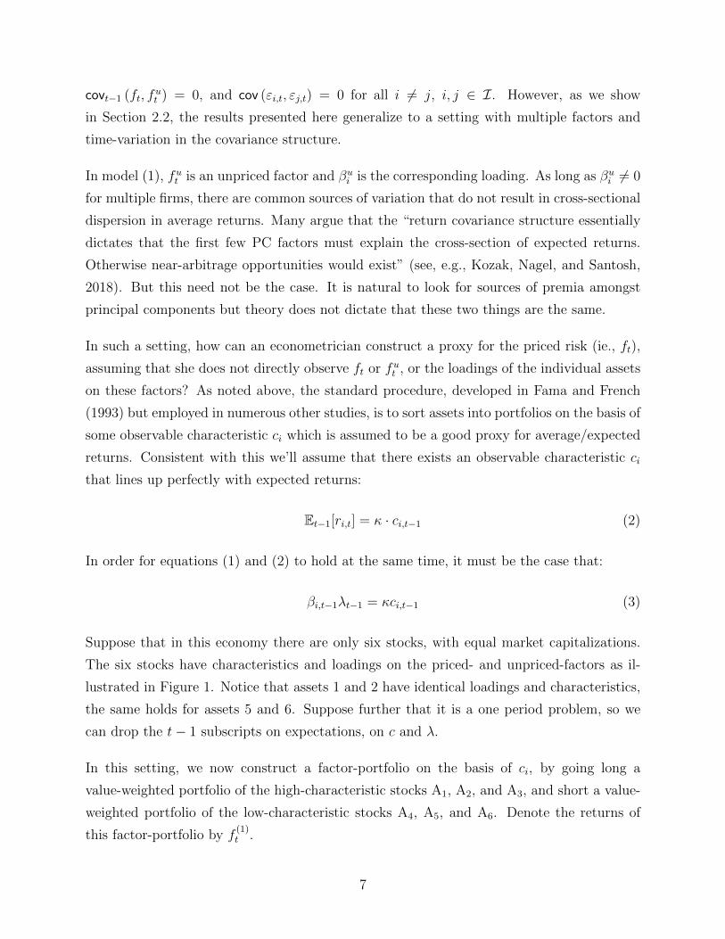
Suppose that in this economy there are only six stocks, with equal market capitalizations.

The six stocks have characteristics and loadings on the priced- and unpriced-factors as il-

lustrated in Figure 1. Notice that assets 1 and 2 have identical loadings and characteristics,

the same holds for assets 5 and 6. Suppose further that it is a one period problem, so we

can drop the t− 1 subscripts on expectations, on c and λ.

In this setting, we now construct a factor-portfolio on the basis of ci, by going long a

value-weighted portfolio of the high-characteristic stocks A1, A2, and A3, and short a value-

weighted portfolio of the low-characteristic stocks A4, A5, and A6. Denote the returns of

this factor-portfolio by f(1)t .

7

6

- βui

βi(= E[ri] = κci

λ

)A1, A2

A3

@@R

A4@

@I

A5, A6

1−1

1

−1

Figure 1: Six assets in the space of loadings and characteristics

Our point here is that, even when the characteristic lines up perfectly with average returns,

there is no guarantee that the returns f(1)t = ft, and therefore that the factor-portfolio will

be mean variance-efficient.

Substituting (3), we can rewrite model 1 as:

Ri,t = κci (ft + λ) + βui fut + εi,t, (4)

To construct a candidate long-short factor portfolio for ft, we buy stocks with high charac-

teristics and short stocks with low characteristics,5 that is:

f(1)t =

1

3×

[3∑j=1

Rj,t −6∑j=4

Rj,t

]= 2κ(ft + λ) +

2

3fut +

1

3

[3∑j=1

εj,t −6∑j=4

εj,t

].

Factor portfolio f(1)t does indeed capture the common source of variation in expected returns,

since it loads on ft . Though, it also loads on the unpriced source of variation fut . The

factor-portfolio f(1)t loads on the factor ft with βf (1) = 2κ, loads on fut with βu

f (1)= 2

3and

5 Because in this simple example all stocks have equal weight there is no difference between equal andvalue weighted. The usual Fama-French construction uses value weighted portfolios.

8

its characteristic is cf (1) = 2. As a result, from equation (4), the expected excess return of

portfolio f(1)t is E

[f(1)t

]= 2κλ and the variance is

var(f(1)t

)= 4κ2σ2

f +4

9σ2fu +

2

3σ2ε .

The Sharpe ratio is thus

SRf (1) =2κλ√

4κ2σ2f + 4

9σ2fu + 2

3σ2ε

(5)

Factor-portfolio f(1)t is not mean variance efficient and thus cannot be the projection of the

stochastic discount factor on the space of returns. To see this, consider forming the following

hedge-portfolio

ht =1

2[R3,t +R6,t]−

1

2[R1,t +R4,t] = −2fut +

1

2[ε3,t + ε6,t]−

1

2[ε1,t + ε4,t] .

This portfolio thus goes long stocks with low loadings and short stocks with high loadings

on fut . Each leg of this portfolio is characteristics balanced. Thus ch = 0 and E [ht] = 0. The

loading of the portfolio ht on fut is βuh = −2. We can use ht to improve on f(1)t . Specifically,

consider the portfolio

f(2)t = f

(1)t − γht. (6)

It is straightforward to show that setting γ = −13

results in a portfolio f(2)t that has a zero

loading on factor fut , βuf (2)

= 0. Moreover

E[f(2)t

]= 2κλ and var

(f(2)t

)= 4κ2σ2

f +7

9σ2ε

and thus a Sharpe ratio of

SRf (2) =2κλ√

4κ2σ2f + 7

9σ2ε

. (7)

Comparing the Sharpe ratios of f(1)t and f

(2)t in equations (5) and (7), respectively, one can

immediately see that if σ2ε is low compared to σ2

fu then SRf (1) << SRf (2) . Notice that given

that the number of assets is finite the investor cannot achieve an infinite Sharpe ratio.6

6In the limit as the number of assets grows SRf(2) →∞.

9

We have chosen γ to eliminate the exposure of f (2) to the unpriced factor fut . In general

though we will choose the parameter γ in order to minimize the variance of the resulting

factor, f(2)t :

minγ

var(f(2)t

)⇒ γ = ρ1,h

σ(f(1)t

)σ (ht)

, (8)

where σ(f(1)t

)is the standard deviation of returns of the original factor-portfolio f

(1)t and

σ (ht) is the standard deviation of the characteristics balanced hedge-portfolio. Setting γ = γ

guarantees that, under the null of model (1), the Sharpe ratio of f(2)t is maximized. In general

then, if model (1) holds, it can be shown that the improvement in the Sharpe ratio of the

original factor-portfolio f(1)t is

SR(2)

SR(1)=

1√1− ρ21,h

. (9)

The question of whether one can improve on the Sharpe ratio associated with exposure to

factor ft is thus an empirical one. In Section 4 we construct hedge-portfolios for each of the

Fama and French (2015) five factors and show that “subtracting them” as in (6) from each

of the factors considerably improves the Sharpe ratio of each of them.

We now formalize further these ideas. Specifically, the next section shows the relation that

exists between the cross sectional correlation of the characteristic used to effect the sort and

the loadings of unpriced factors, on the one hand, and the improvement in the Sharpe ratio

of the portfolio that is proposed as a projection of the priced factor on the space of returns,

on the other.

10

2.2 General Case

2.2.1 Factor representations

Consider setting with N risky assets and a risk-free asset whose returns are generated ac-

cording to a K factor structure:

Rt = βt−1 (ft + λt−1) + εt (10)

where Rt is N×1 vector of the period t realized excess returns of the N assets; ft is a K×1

vector of the period t unanticipated factor returns, with Et−1[ft] = 0, and λt−1 is the K×1

vector of premia associated with these factors. βt−1 is the N ×K matrix of factor loadings,

and εt is the N×1 vector of (uncorrelated) residuals. We assume that N K, and that

N is sufficiently large so that well diversified portfolios can be constructed with any factor

loadings.7

As it is well known, there is a degree of ambiguity in the choice of the factors. Specifically,

any set of the factors that span the K-dimensional space of non-diversifiable risk can be

chosen, and the factors can be arbitrarily scaled. Therefore, without loss of generality, we

rotate and scale the factors so that:8

λt−1 =

1

0...

0

and Ωt−1 = Et−1[ftf ′t] =

σ21 0 · · · 0

0 σ22 · · · 0

......

. . ....

0 0 · · · σ2K

(11)

We further define:

µt−1 = Et−1[Rt] Σεt−1 = Et−1[εtεt′] and Σt−1 = Et−1[RtR

′t] = βt−1Ωt−1β

′t−1 + Σε

t−1

7We note that, in a finite economy, the breakdown of risk into systematic and idiosyncratic is problematic.See Grinblatt and Titman (1983), Bray (1994) and others.

8The rotation is such that the first factor captures all of the premium. The scaling of the first factor is suchthat its expected return is 1. The other factors form an orthogonal basis for the space of non-diversifiablerisk, but the scaling for all but the first factor is arbitrary

11

where µt−1 and σ2ε are N×1 vectors. Given we have chosen the K factors to summarize the

asset covariance structure, Σεt−1 = Et−1[εtε′t] is a diagonal matrix, (i.e., with the residual

variances on the diagonal, and zeros elsewhere).

2.2.2 Characteristic-based factor-portfolios

Over that last several decades, academic studies have documented that certain character-

istics (market capitalization, price-to-book values ratios, past returns, etc.) are related to

expected returns. In response to this evidence, Fama and French (1993; 2015), Carhart

(1997), Pastor and Stambaugh (2003), Frazzini and Pedersen (2014) and numerous other

researchers have introduced “factors-portfolios” based on characteristics. The literature has

then tested whether these characteristic-weighted factor-portfolios can explain the cross-

section of returns, in the sense that some linear combination of the factor-portfolios is mean-

variance-efficient.

Assume that we can identify a vector of characteristics that perfectly captures expected

returns, that is such that: ct−1 = κµt−1 (see (3) above). Moreover ct−1 is an N×1 vector,

that is, a single characteristic summarizes expected returns. Following the usual procedure

we assume that the factor-portfolio is formed based on our single vector of characteristics

ct−1 or to put it differently that the weights of the portfolio are assumed to be proportional to

the characteristic. We normalize this portfolio so as to guarantee that it has a unit expected

return:9

wc,t−1 = κ

(ct−1

c′t−1ct−1

)=

µt−1µ′t−1µt−1

(12)

Note that, given this normalization, w′c,t−1µt−1 = 1, as desired.

9The typical normalization in building factor-portfolios is that they are “$1-long, $1 short” zero investmentportfolios. However since we are dealing with excess returns, this normalization is arbitrary and has no effecton the ability of the factor-portfolios to explain the cross-section of average returns.

12

2.2.3 Relation between the characteristic-based factor-portfolio and the MVE-

portfolio

Assuming no arbitrage in the economy, there exists a stochastic discount factor that prices

all assets, and a corresponding mean-variance-efficient portfolio. In our setting the weights

of the MVE portfolio are:

wMVE,t−1 =(µ′t−1Σ

−1t−1µt−1

)−1Σ−1t−1µt−1, (13)

which have been scaled so as to give the portfolio a unit expected return. The variance

of the portfolio is σ2MVE,t−1 =

(µ′t−1Σ

−1t−1µt−1

)−1, so the Sharpe-ratio of the portfolio is

SRMVE =√µ′t−1Σ

−1t−1µt−1.

Given our scaling of returns, the βs of the risky asset w.r.t the MVE portfolio are equal to

the assets’ expected excess returns:10

βMVE,t−1 =covt−1 (Rt, RMVE,t)

vart−1 (RMVE,t)=

Σt−1wMVE,t−1

wMVE,t−1Σt−1wMVE,t−1= µt−1

We can then project each asset’s return onto the MVE portfolio:

Rt = βMVE,t−1RMVE,t + ut = µt−1RMVE,t + ut (14)

u is the component of each asset’s return that is uncorrelated with the return on the MVE

portfolio, which is therefore unpriced risk.

Given the structure of the economy laid out in equations (10) and (11),

RMVE,t = f1,t + 1

where f1 denotes the first element of f (and the only priced factor). This means that,

referencing equation (14),

βMVE,t−1 = µt−1 = β1,t−1 = κ−1ct−1 (15)

10For the third equality, just substitute wMVE,t−1 from equation (13) into the second.

13

Finally, this means that we can write the residual from the regression in equation (14) as:

ut = βut−1fut + εt (16)

where βut−1 is the N × (K − 1) matrix which is βt−1 with the first column deleted (i.e., the

loadings of the N assets on the K − 1 unpriced factors), and fut is the (K − 1)×1 vector

consisting of the 2nd through Kth elements of ft (i.e., the Unpriced factors).

We will use this projection to study the efficiency of the characteristic-weighted factor-

portfolio. Since both the characteristic-weighted and MVE portfolio have unit expected

returns, the increase in variance in moving from the MVE portfolio to the characteristic

portfolio can tell us how inefficient the characteristic-weighted portfolio is. From equations

(12) and (14), we have:

Rc,t = w′t−1,cRt = RMVE,t + (µ′t−1µt−1)−1µ′t−1ut ⇒

Rc,t −RMVE,t =(µ′t−1µt−1

)−1µ′t−1

[βut−1f

ut + εt

]

Thus given (16)

vart−1(Rc,t −RMVE,t) =K∑k=2

[(c′t−1ct−1)−1(c′t−1β

uk,t−1)︸ ︷︷ ︸

≡γk,c

]2σ2k,t−1 (17)

What is the interpretation of (17)? γk,c is the coefficient from a cross-sectional regression

of the kth (unpriced) factor loading on the characteristic.11 Even though the K factors

are uncorrelated, the loadings on the factors in the cross-section are potentially correlated

with each other, and this regression coefficient could potentially be large for some factors.

Indeed, the necessary and sufficient conditions for the characteristic-sorted portfolio to price

all assets are that

11Note that we get the same expression, up to a multiplicative constant, if we instead regress the unpricedfactor loadings on the the priced factor loadings, or on the expected returns, given the equivalence in equation(15).

14

γk,c = 0 ∀ k ∈ 2, . . . , K.

This condition is unlikely hold even approximately. For example, as we show later, in the

middle of the financial crisis, many firms in the financial sector had a high book-to-market

ratio. Thus, their expected return was high (high µ). However, these firms also had a

high loading on the finance industry factor (σ2k,t−1 was high). Because µt−1 (the expected

return based on the characteristics) and βuk,t−1 (the loading on the unpriced finance industry

factor) were highly correlated, the characteristics-sorted portfolio had high industry factor

risk, meaning that it had a lower Sharpe-ratio than the MVE portfolio. Because σ2k,t−1

was quite high in this period, the extra variance of the characteristic-sorted portfolio was

arguably also large. In Section 4, we show how this extra variance can be diagnosed and

taken into account.

Even though industries are a likely candidate for sources of common variation, the procedure

proposed in this paper has the considerable advantage of being able to improve upon standard

factors, without the need of identifying specifically what the unpriced sources of common

variation are.

2.2.4 An optimized characteristic-based portfolio

It follows from the previous discussion that the optimized characteristic-based portfolio is

w∗c,t−1 = κ

(Σ−1t−1ct−1

c′t−1Σ−1t−1ct−1

)=

Σ−1t−1µt−1

µ′t−1Σ−1t−1µt−1

(18)

Clearly the challenge is the actual construction of such a portfolio. For instance, there are

well known issues associated with estimating Σt−1 and using it to do portfolio formation. In

the next subsection, we develop an alternative approach for testing portfolio optimality.

Assuming the characteristics model is correct, and one observes the characteristics, it is

straightforward to test the optimality of the characteristics-sorted factor-portfolio. All that

is needed is some (ex-ante) instrument to forecast the component of the covariances which

is orthogonal to the characteristics. If the characteristic sorted portfolio is optimal (i.e.,

MVE) then characteristics must line up with betas with the characteristics sorted-portfolio

15

perfectly. If they don’t (and the characteristics model holds) then the portfolio can’t be

optimal.

Moreover, one can improve on the optimality of the portfolio by following the procedure

advocated in this paper, by, first, identifying assets with high (low) alphas relative to the

characteristic-sorted portfolio (again based on the characteristic model) and, second, building

a portfolio with the highest possible expected alpha relative to the characteristic sorted

portfolio, under the characteristic hypothesis. If this portfolio has a positive alpha then

the optimality of the characteristics-sorted portfolio is established. This is the empirical

approach we take in this paper.

In sum, our point is that if a particular characteristic is used to construct a factor-portfolio

then, whenever there is a correlation between the characteristic and the loadings on unpriced

sources of variation, the factor-portfolio will fail to be main variance efficient. Thus the

factor cannot be a proxy for the true, underlying, stochastic discount factor. In the next two

sections, we show that the point is not just of theoretical interest but that its quantitative

importance is substantial. We do so in two different ways. In the next section we focus in

one particular factor, Fama and French (1993) HML factor and show that it loads heavily

on particular industries at particular times. This source of variation is unpriced and thus

one can improve on this factor by removing its dependence of industry factors. In Section 4

we use the more general procedure developed in this section to improve upon the standard

Fama and French (2015) five factors.

3 Sources of common variation: Industry Factors

Asness et al. (2000), Cohen and Polk (1995) and others12 have shown that if book-to-price

ratios are decomposed into an industry-component and a within-industry component, then

only the within-industry component— that is, the difference between a firm’s book-to-price

ratio and the book-to-price ratio of the industry portfolio—forecasts future returns. This

suggests that any exposure of HML to industry factors is likely unpriced. Therefore, if the

industry exposure of HML was hedged out, it would result in a factor-portfolio with lower

risk, but the same expected return, i.e., with a higher Sharpe ratio. But, does HML load on

industry factors?

12See also Lewellen (1999) and Cohen et al. (2003).

16

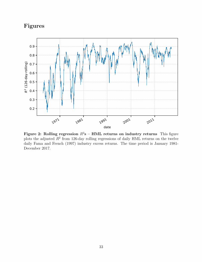
Figure 2 plots the R2 from 126-day rolling regressions of daily HML returns on the twelve

daily Fama and French (1997) value-weighted industry excess returns. The time period is

January 1964 to December 2017.13The plot shows that, while there are short periods where

the realized R2 dips below 50%, there are also several periods where it exceeds 90%. The

R2 fluctuates considerably but the average is well above 70%. The upper Panel of Figure

3 plots, for the same set of daily, 126-day rolling regressions, the regression coefficients for

each of the 12 industries. As it is apparent these coefficients display considerable variation:

sometimes the HML portfolio loads more heavily on some industries than on others.

To provide some clarity, let’s focus on two particular industries: ‘Business Equipment’, which

comprises many of the high technology firms, and ‘Money’ which includes banks and other

financial firms. The two industries are selected because HML had the lowest and highest

exposure, respectively, to them in the post-1995 period. Start with ‘Business Equipment’

and focus in the late 1990s and 2000. As one can see the regression coefficient of HML on this

particular industry started falling in the mid to late 90s, as the “high-tech” sector started

posting impressive returns. These firms were, in addition, heavy on intangible capital which

was not reflected in book. As their book-to-market shrank these companies were classified

into the growth portfolio: the L in HML became a short on high tech companies, which

became to be dominated by ‘Business Equipment’ industry. Simultaneously the volatility

of returns in this industry started increasing consistently around 1997, reaching a peak in

early 2001, as illustrated in Figure 4, which plots the rolling-126 day volatility of returns.14

The annualized volatility of ‘Business Equipment’ returns hovered below 20% for almost two

decades but then shot up in the mid 90s to well above 60%, at the peak of the Nasdaq

cycle. The increase in the absolute value of the regression coefficient and the high volatility

of returns result on the high R2 of the regression of HML on industry factors.

The behavior of the ‘Money’ industry during and after the Great Recession of 2008 is an

even more striking example of the large industry effect on HML. The regression coefficient

associated with ‘Money’ increased dramatically between 2007 and early 2009 as stock prices

for firms in this segment collapsed and quickly became classified as value. 15 As shown in

13The industry classification follow Ken French’s data library at http://mba.tuck.dartmouth.edu/

pages/faculty/ken.french/Data_Library.14Note that for this plot, like the other “rolling” plots in this section, the x-axis label indicates the date

on which the 126-day interval ends.15As shown in Huizinga and Laeven (2009) banks during the crisis used accounting discretion to avoid

writing down the value of distressed assets. As a result the value of bank equity was overstated. The marketknew better and as a result the book-to-market of bank stocks shot up during the crisis.

17

Figure 4 the volatility of returns also increased dramatically. As a result of these two effects,

‘Money’ explained a substantial amount of the variation of HML returns during those years.

Indeed Figure 5 plots the R2 of a regression of the return on HML on the ‘Money’ industry

excess returns. Between late 2008 and late 2010, the R2 was well above 60%. Why was it so

high? As of December 2007, the top 4 firms by market capitalization in the “Money” industry

were Bank of America, AIG, Citigroup and J.P. Morgan. Three of these four were in the large

value portfolio portfolio (Big/High-BM to use the standard terminology). Interestingly, the

one that wasn’t was AIG – it was in the middle portfolio. While the market capitalization

of these firms falls dramatically through 2008, they remain large and, particularly as the

volatility of the returns on the ‘Money’ industry increases, these firms and others like them

drive the returns both of the HML portfolio and the ‘Money’ industry portfolio.

However, there are firms in the ‘Money’ industry that do not have high book-to-market

ratios, even in the depths of the financial crisis. For example, in 2008 US Bancorp (USB)

and American Express (AXP) were both “L” (low book-to-market) firms. Yet both USB

and AXP have large positive loadings on HML at this point in time (see Table 1). The

reason is that both USB and AXP covary strongly with the returns on the ‘Money’ industry,

as does HML at this point in time. We use this variation within the ‘Money’ industry to

construct hedge-portfolios for each of the Fama and French (2015) factors, as illustrated in

the example in the previous section. In particular, we construct a characteristics balanced

hedge-portfolio, h. The short side of the characteristics balanced portfolio features firms

with high loadings on HML and low and high book-to-market, such as American Express

and Citi, respectively. In the example in Figure 1, American Express would be asset A4 and

Citi would be A1. The long side of the characteristics balanced portfolio is comprised of

stocks with low loadings on HML. Then we combine a long position in the HML portfolio

with an appropriately sized position on the characteristics balanced portfolio to hedge the

exposure of the HML portfolio to the ‘Money’ industry, as in expression (6). This procedure

thus succeeds in creating a more efficient “hedged” HML portfolio, one that has the same

expected return, but lower return variance and therefore a higher Sharpe-ratio, than the

original Fama and French (1993) HML portfolio.

18

4 Hedge Portfolios

4.1 Construction

The empirical goal is to construct the best possible hedge-portfolios, as introduced in model

(1). To achieve this, if f(1)t is a well diversified portfolio, we only need to maximize the hedge-

portfolio loading on the unpriced source of common variation, fut . However, in practice we

do observe the factors ft or fut , neither stocks loadings on those factors. We can observe

ex-ante, though, are the characteristics and an estimate of individual stocks loading on a

candidate factor-portfolio. Notice that the loading on a candidate factor-portfolio is a linear

combination of loadings on ft and fut . To disentangle the two from each other, we use a

procedure first introduced by Daniel and Titman (1997). The idea is to use the ex-ante

loading of each stock i on the candidate factor-portfolio f(1)t and construct portfolios that

maximize the loading on f(1)t . At the same time, these portfolios are constructed in such a

way that they have zero exposure to characteristics, and consequently zero expected return if

the characteristic model holds as in equation (2). Effectively, this leads to a portfolio the has

zero loading on the priced factor, and since it is correlated with candidate factor-portfolio,

it must be the case that is has a non-zero loading on the unpriced factor. Thereby it can be

used to hedge out unpriced risk.

In our empirical exercise, we focus on the five factor Fama and French (2015) model and we

follow these authors in the construction of their factor-portfolios. In the following, we will

explain the procedure based on the example of HML. We first rank NYSE firms by their, in

this case, book-to-market (BEME) ratios at the end of December of a given year and their

market capitalization (ME) at the end of June of the following year. Break points are selected

at the 33.3% and 66.7% marks for both the book-to-market and market capitalization sorts.

Then in June of a given year all NYSE/Amex and Nasdaq stocks are placed into one of the

nine resulting bins. There is an important difference though in the way the sorting procedure

is implemented relative to Fama and French (1992, 1993 and 2015) or Daniel and Titman

(1997) and it is that our characteristics sorted portfolios are industry adjusted. That is,

whether a stock has, for example, a high or low book-to-market ratio depends on whether it

19

is above or below the corresponding value-weighted industry average.16 Our industries are

the 49 industries of Fama and French (1997).

Next, each of the stocks in one of these nine bins is sorted into one of three additional bins

formed based on the stocks’ expected future loading on the HML factor-portfolio. This last

sort results in portfolios of stocks with similar characteristics (BEME and ME) but different

loadings on HML. The firms remain in those portfolios between July and June of next year.

Finally, we construct our hedge-portfolio for the HML factor-portfolio, as in the example in

section 2, by going long an equal-weight combination of all low-loading portfolios and short

an equal-weight combination of all high-loading portfolios. Thereby, the long and short sides

of this portfolio have zero exposure to the characteristic and we maximize the spread in

expected loading on the unpriced sources of common variation.

The hedge-portfolios for RMW and CMA are constructed in exactly the same way. For

SMB, we follow Fama and French (2015) and construct three different hedge-portfolios: one

where the first sorts are based on BEME and ME, and then within these 3x3 bins, we

conditionally sort on the loading on SMB. The second and third versions use OP and INV

instead of BEME in the first sort. Then, an equal weighted portfolio of the three different

SMB hedge-portfolios is used as the hedge-portfolio for SMB. We do exactly the same for

the hedge-portfolio for the market.

Clearly a key ingredient of the last step of the sorting procedure is the estimation of the

expected loading on the corresponding factor. Our purpose is to obtain estimates of the

future loadings in the five factor model of Fama and French (2015):

Ri,t −RF,t = ai,t−1 + βMkt−RF,i,t−1(RMkt,t −RF,t) + βSMB,i,t−1RSMBt

+βHML,i,t−1HMLt + βRMW,i,t−1RMWt + βCMA,i,t−1CMAt + ei,t(19)

We instrument future expected loadings with pre-formation loadings of each stock with the

candidate factor-portfolios. The resulting estimation method is intuitive and is close to the

method proposed by Frazzini and Pedersen (2014). These authors build on the observation

that correlations are more persistent than variances 17 and propose estimating covariances

16The reason we use industry adjusted characteristics is because they have been shown to be better proxiesof expected returns (see Cohen et al. (2003)).

17see, among others, de Santis and Gerard (1997)

20

and variances separately and then combine these estimates to produce the pre-formation

loadings. Specifically, covariances are estimated using a five-year window with overlapping

log-return observations aggregated over three trading days, to account for non-synchronicity

of trading. Variances of factor-portfolios and stocks are estimated on daily log-returns over

a one-year horizon. In addition, we introduce an additional intercept in the pre-formation

regressions for returns in the six months preceding portfolio formation, i.e., from January to

June of the rank-year (see Figure 1 in Daniel and Titman (1997) for an illustration). We refer

to this estimation methodology as the ‘high power’ methodology. Intuitively, if our forecasts

of future loadings are very noisy, then sorting on the basis of forecast-loading will produce no

variation in the actual ex-post loadings of the sorted portfolios. In contrast, if the forecasts

are accurate, then our hedge-portfolio—which goes long the low-forecast-loading portfolio-

and short the high-forecast-loading portfolio—will indeed be strongly correlated with the

corresponding FF portfolio. Also, since this portfolio is “characteristic-balanced”, meaning

the long and short-sides of the portfolio have equal characteristics and, if the characteristic

model is correct, will have zero expected excess return. Such a portfolio would be an optimal

hedge-portfolio, in that it maximizes the correlation with the FF portfolio subject to the

constraint that it is characteristic neutral. Also, such a portfolio would have the highest

possible likelihood of rejecting the FF model, under the hypothesis that the characteristic

model is correct.

The estimation method implemented here contrasts with the one used by Daniel and Titman

(1997) or Davis, Fama, and French (2000) in various aspects. The traditional approach use as

instruments for future factor loadings the result of regressing stock excess returns on factor-

portfolios over a moving fixed-sized window based on, e.g., 36 or 60 monthly observations,

skipping the most recent 6 months18. In addition, this set of hedge-portfolios is not industry

adjusted. We refer to this method, which is effectively the one used by Daniel and Titman

(1997), as the ‘low power’ method and use it to construct an alternative set of hedge-

portfolios.

In sum, the high and low power sets of hedge-portfolios differ in two dimensions: the estima-

tion method for the expected loading and whether the characteristics are industry adjusted

or not. In what follows, we examine to what extent these portfolios differ and whether we

succeed in maximizing our ability to hedge out unpriced sources of common variation.

18Notice that in contrast, the high power method avoids discarding the most recent data.

21

4.2 Average returns and characteristics of triple-sorted portfolios

Table 2 presents average monthly excess returns for the portfolios that we combine to form

our hedge-portfolios. Each panel presents a set of sorts with respect to size and to one

characteristic—either value (Panel A), profitability (Panel B) or investment (Panel C)—and

the corresponding loading.

For example, to form the 27 portfolios in Panel A, we first perform independent sorts of

all firms in our universe into three portfolios based on book-to-market (BEME) and based

on size (ME) NYSE breakpoints. . We then sort each of these nine portfolios into three

sub-portfolios, each with an equal number of firms, based on the ex-ante forecast loading

on HML for each firm. In the upper subpanels, the loading sorts are estimated using the

low-power methodology; and in the lower panels using the high-power methodology.

For each of the 27 portfolios in each subpanel, we report value-weighted monthly excess

returns. The column labeled “Avg.” gives the average across the 9 portfolios for a given

characteristic.

First, note that the average returns in the “Avg.” column are consistent with empirical

regularities well known in the literature: the average returns of value portfolios are higher

than those of growth, historically profitable firms beat unprofitable, and historically low

investment firms beat high investment firms. In Table 4 we present the ex-post loadings. We

see that there are large differences between the ex-post betas of the low-forecast-loading (“1”)

and high-forecast-loading (“3”) portfolios for every size-characteristic portfolio, particularly

when these sorts are done using the high-power-methodology. For the value, profitability, and

investment sorts, the ex-post differences in loading of the “3” and “1” portfolios are 0.94, 0.77,

and 1.09 respectively. Given these large differences in loadings for the high-power sorts, it is

remarkable that the difference in the average monthly returns for the high- and low-loading

portfolios are 7, 14, and 2 bp/month for the value, profitability and investment-loading sorts,

respectively.19 This is consistent with the Daniel and Titman (1997) conjecture that average

returns are a function of characteristics, and are unrelated to the FF factor loadings after

controlling for the characteristics.

19For comparison, the average excess returns of the HML, RMW, and CMA portfolios over the same periodare 34, 28, and 23 bp/month, respectively.

22

Moreover, these small observed return differences may be related to the fact that, in sorting

on factor loadings, we are picking up variation in characteristics within each of the nine size-

characteristic-sorted portfolios. For example, among the firms in the small-cap, high book-to-

price portfolios in Panel A, there is considerable variation in book-to-market ratios. In sorting

into sub-portfolios on the basis of forecast HML-factor loading, we are undoubtedly picking

up variation in the characteristic of the individual firms, since characteristics and factor-

loadings are highly correlated (i.e, value firms typically have high HML factor loadings).

We explore this possibility in Table 3, where we show the average of the relevant characteristic

for each of the portfolios. Consistent with our hypothesis, there is generally a relation

between factor loadings and characteristics within each of the nine portfolios.

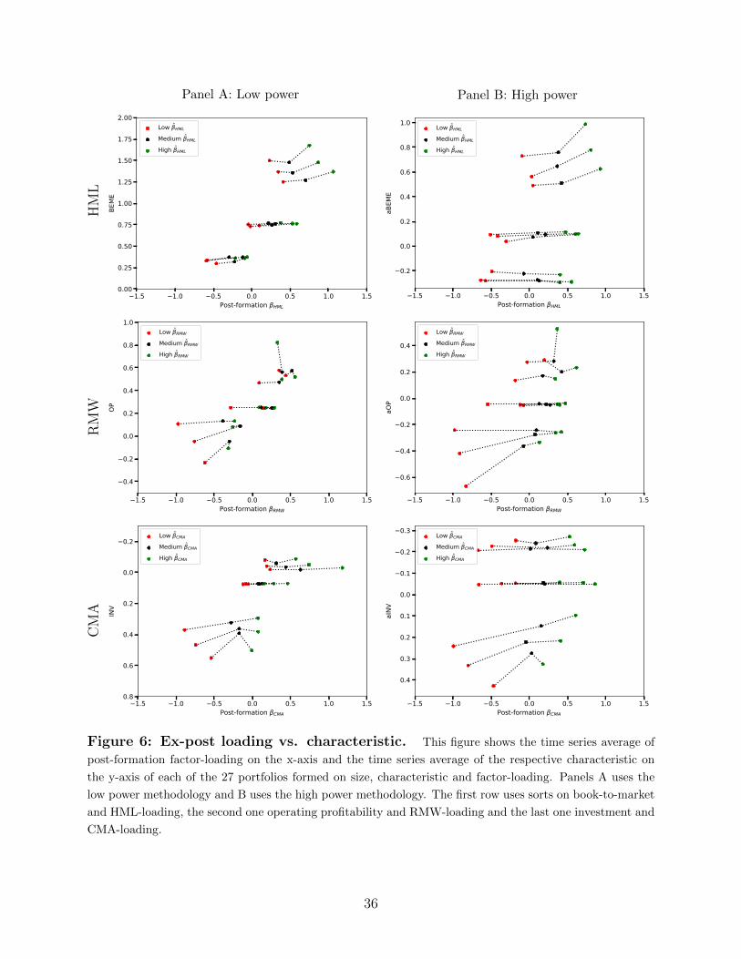
4.3 Postformation loadings

We estimate the post-formation loadings by running a full-sample time series regression of the

monthly excess returns for each of the portfolios on the Fama and French (2015) five factors

(see equation (19)). To compare whether our high power methodology results in larger

dispersion of the post-formation loadings when compared to the low power methodology,

Figure 6 shows the postformation loadings for each of the 27 portfolios. Panels A and B

correspond to the low and high power methodology, respectively.

Consider for example the top panels in Figure 6, which focus on the loadings on HML for

each of the two estimation methodologies. There are 3×3 groups of estimates—connected by

lines—each corresponding to a particular book-to-market × size bin. Each of those lines have

three points corresponding to the three portfolios from the conditional sort on ex-ante betas.

The plot thus reports book-to-market on the y-axis for each of the 27 portfolios and the

post-formation loading on the x-axis. The actual point estimates for the loadings on HML,

together with the corresponding t-statistics, are reported in Table 4 Panel A. To illustrate

the point further focus on the loadings on HML for the large value portfolios (portfolio

(3,3)). The low power methodology generates post-formation loadings on HML, βHML, for

each of the three portfolios of 0.41, 0.7 and 1.06, respectively. The high power methodology

instead generates post-formation HML loadings of 0.05, 0.42 and 0.93, respectively. The last

column of the panel reports the post-formation loading on HML of the portfolio that goes

long the low loading portfolio and short the high loading portfolio amongst the large value

23

firms, portfolio. The loading is −0.65 for the low power methodology with a t−statistic of

−9.19. For the high power methodology the same post-formation loading is −0.88 with a

t−statistic of −12.69.

Notice that, reassuringly, both methodologies generate a positive correlation between pre-

and post-formation loadings for each of the book-to-market and size groupings. This positive

correlation between pre- and post extents to the case of CMA. But in the case of the loadings

on RMW, the low power methodology does not produce a consistent positive association

between pre- and post-formation loadings, whereas the high power methodology does. Indeed

turn to Table 4 Panel B, which reports the post-formation loadings20 on the profitability

factor, RMW, and focus on the portfolios (3,1), that is small firms with high operating

profitability. The low power methodology generates loadings of 0.35, 0.39 and 0.33, a non-

monotone relation. Instead the post-formation loadings for the same set of portfolios as

estimated by the high-power methodology are −0.03, 0.32 and 0.36.

As it is readily apparent from Figure 6, the high power methodology generates substantially

more cross sectional dispersion in post-formation loadings than the low power methodology,

which is key to generating hedge-portfolios that are maximally correlated with the can-

didate factor. Each of the panels of Table 4 reports the difference in the post-formation

loadings between the low and and high pre-formation loading sorted portfolio for each of

the characteristic-size bin. Consistently, this difference is much larger with the high power

methodology than the low. In sum then our high power methodology forecasts future load-

ings better than the one used by Daniel and Titman (1997) or Davis et al. (2000) and, as a

result, they translate into more efficient hedge-portfolios as well as asset pricing tests with

higher power.

5 Empirical Results

In this section we describe the two main empirical results of this paper. First we show

how the use of the high power methodology advanced in this paper to forecast loadings

increases the power of standard asset pricing tests. We illustrate how the standard low

power methodology used to estimate the loadings lead to a failure to reject asset pricing

20The alphas of these regressions are also reported in Table 4. We will turn to the asset pricing implicationsin Section 5.1.

24

models and thus impose too low a bound on the volatility of the stochastic discount factor.

We do so by constructing characteristics balanced portfolios and showing that the ability of

standard asset pricing models to properly account for their average returns depends critically

on whether one uses the low or high power methodology.

Our second contribution is to show how to improve the Sharpe ratios of factor-portfolios

by combining them optimally with the hedge-portfolios. We argue that these hedged factor-

portfolios have a better chance of spanning the mean variance frontier than the standard

factor models proposed in the literature.

5.1 Pricing the characteristics balanced hedge-portfolios

We turn now to the characteristics balanced hedge-portfolios. We construct them as follows:

for each of the five factors in the Fama and French (2015) model we form a portfolio that goes

long the portfolios with low loading forecast on the corresponding factor, averaging across

the corresponding characteristic and size, and short the high loading forecast portfolios. For

instance consider the line labeled HML in Table 5. There, we take a long position in the low

loading portfolios, weighting the corresponding nine book-to-market size sorted portfolios

equally, and a short position in the nine high loading portfolios in the same manner.

We then run a single time series regression of the returns of these hedge-portfolios hk,t on the

five Fama and French (2015) factor-portfolios. Table 5 reports the alphas and loadings as

well as the corresponding t−statistics. Panel A focuses on the set of hedge-portfolios where

pre-formation loadings are estimated with the low power methodology and Panel B focuses

on the high power one. We first assess the hedge-portfolios’ ability to hedge out unpriced risk

by looking at their post-formation loading on the corresponding factor. As expected, each

hedge-portfolio exhibits a strong negatively significant loading on their corresponding factor.

For example, the hedge-portfolio for HML has a loading on HML of −0.49 with a t−statistic

of −17.02, for the low power methodology. All of these numbers are larger in magnitude

for the high power methodology - in the case of HML, the loading is −0.94 now, with a

t−statistic of −35.96. To check whether these are unpriced, as was intended by constructing

the portfolios to be characteristic-neutral, we turn to the average realized excess-return of

the test-portfolios. It is statistically indistinguishable from zero for all hedge-portfolios.

25

This directly translates into pricing implications, as indicated by the alphas. Whereas,

when using the low-power methodology, the five Fama and French factors price all hedge-

portfolios correctly, the model fails to price four out of five of the high-power long-short

hedge-portfolios.21 The last line of each of the panels constructs equal weighted combinations

of these portfolios. The alphas for all of them are strongly statistically significant in the high

power test whereas this is not the case for the low power methodology. For instance, when we

consider the equal-weight combination of four factors (HML,RMW, CMA and the market),

the monthly alpha is 0.19 with a t-statistic of 6.18.

5.2 Ex-ante determination of the optimal hedge-ratio

Now that the hedge-portfolios’ effectiveness to hedge out unpriced risk is established, the

next step is to construct improved or hedged factors, i.e.,

f(2)k,t = f

(1)k,t − γ

′k,t−1ht

where k ∈ HML,RMW,CMA,SMB,MktRF.

The optimal hedge ratio γk,t−1 is determined ex-ante, in the spirit of equation (8). We

employ the same loading forecast techniques as described before to forecast γk,t−1, i.e., we

first calculate five years of constant weight and constant allocation pre-formation returns of

f(1)k,t and ht. We then calculate correlations over the whole five years of 3-day overlapping

return observations and variances by utilizing only the most recent 12 months of daily obser-

vations. Note that this is done in a multi-variate framework, i.e., we consider the covariance

of each candidate factor-portfolio with all five hedge-portfolios, to account for the correla-

tion structure among the hedge-portfolios. Consequently, both γk,t−1 and ht are length-K

vectors, where K=5 in the case of the Fama and French model examined here. Note further,

that the factor-portfolios f(2)k,t are (approximately) orthogonal to the hedged portfolios hk,t.

The reason why they are only approximately orthogonal is because the γk,t−1 is estimated

ex-ante, i.e., up to t− 1.

21The only one for which the Fama and French model cannot be rejected is the “SMB” portfolio. The factthat Fama and French model succeeds in pricing hSMB is consistent with the notion that there is little toprice there, as we know that the size premium is relatively weak.

26

5.3 Hedged Fama and French Factor Portfolios

Table 6 reports key statistics on the unhedged (f(1)t ) and hedged (f

(1)t ) versions of the five

factors. For each of the five Fama and French (2015) factors we report the annualized

average returns in percentages, the annualized volatility of returns and the Sharpe ratio.

The second column reports the same three quantities for the improved factor-portfolios,

f(2)t . These portfolios are constructed exactly as in expression (6).22

When we move from f(1)k,t to f

(2)k,t , we see that the mean return of all factors decreases, but the

volatility also decreases considerably more. This leads to an increase in the Sharpe ratio for

each of the individual Fama and French factor-portfolios. For example, the squared Sharpe

ratio of the improved version of HML is 0.31, where the original HML factor’s squared Sharpe

ratio is 0.17.

While the result that we improve on each factor-portfolio individually is promising, the

ultimate goal of the exercise was to move the candidate factor representation of the stochastic

discount factor closer to being mean-variance efficient. Hence, in the bottom panel of Table

6, we compute the in-sample optimal combination of both the original Fama and French

factors (column f(1)k,t ) and the improved versions (f

(2)k,t ). The maximum achievable squared

Sharpe ratio with the original Fama and French factors in the sample period covered in this

paper (1963/07 - 2017/12) turns out to be 1.3. The squared Sharpe ratio of the optimal

combination of the improved versions of these five factors is 2.25.23

Notice that each individual improved factor-portfolio f(2)k,t is perfectly tradable, as all infor-

mation used to construct them is known to an investor ex-ante. Only the weights of optimal

combinations of the five (traditional as well as improved) factor-portfolios, as reported in

the bottom panel of Table 6, are calculated in-sample. Additionally, we want to emphasize

that the way we construct our portfolios is very conservative, in that we only rebalance once

every year—in order to be consistent with the rules of the game set by Fama and French.

22 We calculate the Sharpe ratio of the factor-portfolio f(2)t using the usual procedure rather than using

expression (9), which only holds under the null of model (1).23 We can reject the hypothesis of equal Sharpe ratios with a p-value of 0.01, using the time-series bootstrap

procedure of Ledoit and Wolf (2008) with 5000 draws and a block-length of 6.

27

5.4 Redundancy of HML

Fama and French (2015) find that HML is redundant, in that it is spanned by the other factor

portfolios. Table 7 shows that we can replicate this result based on our extended sample.

The weight of HML in the ex-post optimal combination, based on Markowitz optimization, is

-1.0 % when we use the original Fama and French (2015) five factors (column f(1)k ). However,

if we use the improved five factors (column f(2)k ), HML’s weight increases to 12.0 %, roughly

as big as the weight on the market and SMB.

We can confirm this result by running spanning regressions in Table 8. The original HML is

indeed spanned by the other four factor portfolios (column 1). It is similarly subsumed by

the other four improved factors (column 2). The improved version of HML (columns 3 and

4) can neither be explained by the original nor the improved four other factors. Hence, the

improved version of HML is not redundant anymore.

5.5 Industry Neutral Factor-Portfolios

In Section 3, we saw that industry is one source of common variation that is likely to be

unpriced. Since we know that there are periods that the Fama and French factor-portfolios

strongly load on industry portfolios, a natural exercise is to construct factor-portfolios that

are industry-neutral. In this section, we construct an industry neutral version of factor-

portfolios and compare how they perform in comparison to the improved factors constructed

in this paper.

To construct industry-neutral factor-portfolios, denoted by f INk , we ex-ante hedge out any

exposure to the 12 industries of all 5 factors. f INk is defined as:

f INk = fk,t − β′k,t−1fINDt , (20)

where k ∈ HML,RMW,CMA,SMB,MktRF, f INDt is a (12 × 1) vector with excess

returns of all 12 industries, βk,t−1 is the ex-ante optimal industry hedge. Analogous to the

previous exercises, βk,t−1 is estimated every July 1st, using correlations over the previous

five years of 3-day overlapping return observations and variances by using only the most

recent 12 months of daily observations. To calculate correlations and variances, portfolios

28

weights for both industry and factor portfolios are held constant as of the portfolio formation

date.

We also calculate a second iteration of industry neutral factor-portfolios, denoted by fIN(2)k ,

in which we apply the methodology described in Section 4 having as stating point f INk . The

objective is to analyze if there is scope to improve the f INk by hedging out unpriced risk, even

if, the original factor-portfolios are industry neutral and, by construction, industry cannot

be the source of unpriced risk.

In the last two columns of Table 6, we present the mean, volatility and squared Sharpe ratio

for all f INk and fIN(2)k and the in-sample optimal combination of the 5 factors for each case.

The first thing to note is that even though hedging industry leads to an improvement in the

squared Shape-ratio of HML and CMA, the same is not true for other factors. Furthermore,

for all factor-portfolios, except HML, the f (2) outperforms f IN . We conclude that f (2)

outperforms f IN by looking at in-sample optimal combination. Whereas hedging unpriced

risk leads to a squared Share-ratio of 2.25, ex-ante hedging out industry exposure leads to

an in-sample optimal squared Sharpe ratio of 1.46. Finally, the fIN(2)k column shows that

we can improve industry neutral factor-portfolios by applying our procedure to hedge out

additionl unpriced risk. This increases the squared Shape-ratio from 1.46 to 1.59.

These results suggest that simply hedging out industry exposure might not be optimal.

There are at least two interpretations for this result. One interpretation is that the industry

factors can be decomposed into a priced and an unpriced part. By creating industry-neutral

portfolios, we indistinguishably hedge out both components, thereby causing a strong de-

crease in the mean of the factor-portfolios. Second, there can be other sources of common

variation that are not related to industries and do not command a premium. The results

of this sections suggest that the hedge-portfolios constructed in Section 4 are superior in

identifying and hedging out sources of unpriced risk.

6 Conclusions

A set of factor-portfolios can only explain the cross-section of average returns if the mean-

variance efficient portfolio is in the span of these factor-portfolios. There are numerous

sources of information from which to construct such a set of factors. In the cross-sectional

29

asset pricing literature, the most widely utilized source of information used to form factor-

portfolios have been observable firm characteristics such as the ones we examine here: firm

size, book-to-market ratio, and accounting-based measures of profitability and investment.

Portfolios formed going long high-characteristic firms and short low-characteristic firms ig-

nore the forecastable part of the covariance structure, and thus cannot explain the returns

of portfolios formed using the characteristics and past-returns. Factor-portfolios formed in

this way are therefore inefficient with respect to this information set.

In the empirical part of this paper, we have examined one particular model in this literature:

the five-factor model of Fama and French (2015). Our empirical findings show that the

factor-portfolios that underlie this model contain large unpriced components, which we show

are at least correlated with unpriced factors such as industry risk. When we add information

from the historical covariance structure of returns we can vastly improve the efficiency of

these factor-portfolios, generating a portfolio that is orthogonal to the original five factors

and has a squared Sharpe-ratio of 2.25 − 1.3 = 0.95. It is important to note that we are

extremely conservative in the way in which we construct these hedged-portfolios: following

Fama and French (1993), we form portfolios annually, and value-weight these portfolios.

By hedging out the ex-ante identifiable, unpriced risk in the five-factors, we increase the

annualized squared-Sharpe ratio achievable with these factors.

Hedged factor-portfolios like those we construct here raise the bar for standard asset pricing

tests. By the logic of Hansen and Jagannathan (1991), a pricing kernel variance of at least

2.25 (annualized) is required to explain the returns of the hedged-factor-portfolios. Also,

because the hedged factor-portfolios are far less correlated with industry factors, etc., they

are also far less likely to be correlated with variables that might serve as plausible proxies

for marginal utility.

In addition, the hedged factor-portfolios we generate can serve as an efficient set of bench-

mark portfolios for doing performance measurement using Jensen (1968) style time-series

regressions. Such an approach will deliver the same conclusions as the characteristics ap-

proach (Daniel, Grinblatt, Titman, and Wermers, 1997), while maintaining the convenience

of the factor regression approach.

30

References

Asness, Clifford S, Andrea Frazzini, and Lasse H Pedersen, 2013, Quality minus junk, AQRCapital Management working paper.

Asness, Clifford S., R. Burt Porter, and Ross Stevens, 2000, Predicting stock returns usingindustry-relative firm characteristics, SSRN working paper # 213872.

Bray, Margaret, 1994, The Arbitrage Pricing Theory is not Robust 1: Variance Matrices andPortfolio Theory in Pictures (LSE Financial Markets Group).

Carhart, Mark M., 1997, On persistence in mutual fund performance, Journal of Finance52, 57–82.

Cohen, Randolph B., Christopher Polk, and Tuomo Vuolteenaho, 2003, The value spread,The Journal of Finance 58, 609–642.

Cohen, Randolph B., and Christopher K. Polk, 1995, An investigation of the impact ofindustry factors in asset-pricing tests, University of Chicago working paper.

Daniel, Kent D., Mark Grinblatt, Sheridan Titman, and Russ Wermers, 1997, Measuringmutual fund performance with characteristic-based benchmarks, Journal of Finance 52,1035–1058.

Daniel, Kent D., and Sheridan Titman, 1997, Evidence on the characteristics of cross-sectional variation in common stock returns, Journal of Finance 52, 1–33.

Daniel, Kent D., and Sheridan Titman, 2012, Testing factor-model explanations of marketanomalies, Critical Finance Review 1, 103–139.

Davis, James, Eugene F. Fama, and Kenneth R. French, 2000, Characteristics, covariances,and average returns: 1929-1997, Journal of Finance 55, 389–406.

de Santis, Giorgio, and Bruno Gerard, 1997, International asset pricing and portfolio diver-sification with time-varying risk, The Journal of Finance 52, 1881–1912.

Fama, Eugene F., and Kenneth R. French, 1993, Common risk factors in the returns onstocks and bonds, Journal of Financial Economics 33, 3–56.

Fama, Eugene F., and Kenneth R. French, 1997, Industry costs of equity, Journal of Finan-cial Economics 43, 153–193.

Fama, Eugene F., and Kenneth R. French, 2010, Luck versus skill in the cross-section ofmutual fund returns, The Journal of Finance 65, 1915–1947.

Fama, Eugene F., and Kenneth R. French, 2015, A five-factor asset pricing model, Journalof Financial Economics 116, 1–22.

Frazzini, Andrea, and Lasse H. Pedersen, 2014, Betting against beta, Journal of FinancialEconomics 111, 1–25.

31

Grinblatt, Mark, and Sheridan Titman, 1983, Factor pricing in a finite economy, Journal ofFinancial Economics 12, 497–507.

Hansen, Lars P., and Ravi Jagannathan, 1991, Implications of security market data formodels of dynamic economies, Journal of Political Economy 99, 225–262.

Jensen, Michael C, 1968, The performance of mutual funds in the period 1945-1964, Journalof Finance 23, 389–416.

Kozak, Serhiy, Stefan Nagel, and Shrihari Santosh, 2018, Interpreting factor models, TheJournal of Finance 73, 1183–1223.

Ledoit, Oliver, and Michael Wolf, 2008, Robust performance hypothesis testing with theSharpe ratio, Journal of Empirical Finance 15, 850–859.

Lewellen, Jonathan, 1999, The time-series relations among expected return, risk, and book-to-market, Journal of Financial Economics 54.

Lewellen, Jonathan, Stefan Nagel, and Jay Shanken, 2010, A skeptical appraisal of assetpricing tests, Journal of Financial Economics 96, 175–194.

Lustig, Hanno N., Nikolai L. Roussanov, and Adrien Verdelhan, 2011, Common risk factorsin currency markets, Review of Financial Studies 24, 3731–3777.

Markowitz, Harry M., 1952, Portfolio selection, Journal of Finance 7, 77–91.

Pastor, Lubos, and Robert F. Stambaugh, 2003, Liquidity risk and expected stock returns,Journal of Political Economy 111, 642–685.

Roll, Richard W., 1977, A critique of the asset pricing theory’s tests, Journal of FinancialEconomics 4, 129–176.

32

Figures

Figure 2: Rolling regression R2s – HML returns on industry returns This figureplots the adjusted R2 from 126-day rolling regressions of daily HML returns on the twelvedaily Fama and French (1997) industry excess returns. The time period is January 1981-December 2017.

33

Figure 3: HML loadings on industry factors. The upper panel of this figure plotsthe betas from rolling 126-day regressions of the daily returns to the HML-factor portfolioon the twelve daily Fama and French (1997) industry excess returns over the January 1964-December 2017 time period. The lower panel plots only the betas for the Money and BusinessEquipment industry portfolios, and excludes the other 10 industry factors.

34

Figure 4: Volatility of the money and business equipment factors. This figure plots

126-day volatility of the daily returns to the Money and the Business Equipment factors over the January

1964-June 2017 time period.

Figure 5: Rolling regression R2s – HML returns on Money industry returns.This figure plots the adjusted R2 from 126-day rolling regressions of daily HML returns on the daily Money

industry returns from the 12 Fama and French (1997) industry returns. The time period is January 2000-

December 2017.35

HM

LPanel A: Low power

1.5 1.0 0.5 0.0 0.5 1.0 1.5Post-formation HML

0.00

0.25

0.50

0.75

1.00

1.25

1.50

1.75

2.00BE

ME

Low HML

Medium HML

High HML

Panel B: High power

1.5 1.0 0.5 0.0 0.5 1.0 1.5Post-formation HML

0.2

0.0

0.2

0.4

0.6

0.8

1.0

aBEM

E

Low HML

Medium HML

High HML

RM

W

1.5 1.0 0.5 0.0 0.5 1.0 1.5Post-formation RMW

0.4

0.2

0.0

0.2

0.4

0.6

0.8

1.0

OP

Low RMW

Medium RMW

High RMW

1.5 1.0 0.5 0.0 0.5 1.0 1.5Post-formation RMW

0.6

0.4

0.2

0.0

0.2

0.4

aOP

Low RMW

Medium RMW

High RMW

CM

A

1.5 1.0 0.5 0.0 0.5 1.0 1.5Post-formation CMA

0.2

0.0

0.2

0.4

0.6

0.8

INV

Low CMA

Medium CMA

High CMA

1.5 1.0 0.5 0.0 0.5 1.0 1.5Post-formation CMA

0.3

0.2

0.1

0.0

0.1

0.2

0.3

0.4

aINV

Low CMA

Medium CMA

High CMA

Figure 6: Ex-post loading vs. characteristic. This figure shows the time series average of

post-formation factor-loading on the x-axis and the time series average of the respective characteristic on

the y-axis of each of the 27 portfolios formed on size, characteristic and factor-loading. Panels A uses the

low power methodology and B uses the high power methodology. The first row uses sorts on book-to-market

and HML-loading, the second one operating profitability and RMW-loading and the last one investment and

CMA-loading.

36

Figure 7: Portfolio Cumulative Returns. This figure plots the cumulative returnsof of the five FF(2015) portfolios, and the residual portfolio. The residual portfolio is theequal-weighted combination of the HML, RMW, and CMA hedge portfolios, orthogonalizedto the five-factors. Each portfolio assumes an investment of $1 at close on the last tradingday of June 1963, and earns a return of (1 + rLS,t + rf,t) in each month t, where rLS,t is thelong-short portfolio return, and rf,t is the one month risk free rate.

37

Tables

Table 1: Low book-to-market stocks in the Money industry as of June 2008.The first column reports the largest fifteen stocks in the Money industry in the low book-to-market bin

by market capitalization. The second column reports the book-to-market and the third reports the HML

loading portfolio to which the stock belongs as of June 30th, 2008.

Firm BE/ME βHML-portfolioUS Bancorp 0.39 3American Express 0.19 3United Health 0.27 2Aflac 0.36 2State Street 0.36 2Charles Schwab 0.13 1Franklin Resources 0.27 3Aetna 0.36 1American Tower 0.18 3Northern Trust 0.30 3Price T. Rowe 0.17 2Progressive 0.38 3Crown Castle 0.29 3TD Ameritrade 0.21 2Cigna 0.34 1

38

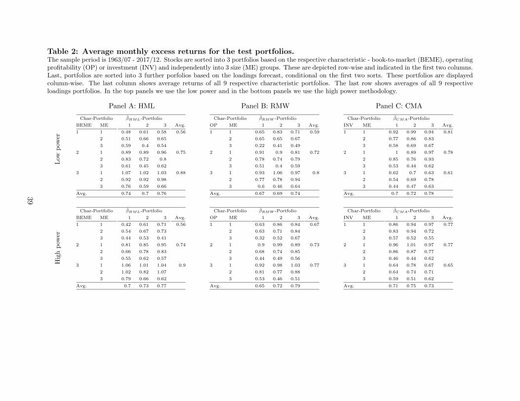
Table 2: Average monthly excess returns for the test portfolios.The sample period is 1963/07 - 2017/12. Stocks are sorted into 3 portfolios based on the respective characteristic - book-to-market (BEME), operatingprofitability (OP) or investment (INV) and independently into 3 size (ME) groups. These are depicted row-wise and indicated in the first two columns.Last, portfolios are sorted into 3 further porfolios based on the loadings forecast, conditional on the first two sorts. These portfolios are displayedcolumn-wise. The last column shows average returns of all 9 respective characteristic portfolios. The last row shows averages of all 9 respectiveloadings portfolios. In the top panels we use the low power and in the bottom panels we use the high power methodology.

Low

pow

er

Panel A: HML

Char-Portfolio βHML-Portfolio

BEME ME 1 2 3 Avg.

1 1 0.48 0.61 0.58 0.56

2 0.51 0.66 0.65

3 0.59 0.4 0.54

2 1 0.89 0.89 0.96 0.75

2 0.83 0.72 0.8

3 0.61 0.45 0.62

3 1 1.07 1.02 1.03 0.88

2 0.92 0.92 0.98

3 0.76 0.59 0.66

Avg. 0.74 0.7 0.76

Panel B: RMW

Char-Portfolio βRMW -Portfolio

OP ME 1 2 3 Avg.

1 1 0.65 0.83 0.71 0.59

2 0.65 0.65 0.67

3 0.22 0.41 0.49

2 1 0.91 0.9 0.81 0.72

2 0.78 0.74 0.79

3 0.51 0.4 0.59

3 1 0.93 1.06 0.97 0.8

2 0.77 0.78 0.94

3 0.6 0.46 0.64

Avg. 0.67 0.69 0.74

Panel C: CMA

Char-Portfolio βCMA-Portfolio

INV ME 1 2 3 Avg.

1 1 0.92 0.99 0.94 0.81

2 0.77 0.86 0.83

3 0.58 0.69 0.67

2 1 1 0.89 0.97 0.78

2 0.85 0.76 0.93

3 0.53 0.44 0.62

3 1 0.62 0.7 0.63 0.61

2 0.54 0.69 0.78

3 0.44 0.47 0.63

Avg. 0.7 0.72 0.78

Hig

hp

ower

Char-Portfolio βHML-Portfolio

BEME ME 1 2 3 Avg.

1 1 0.42 0.61 0.71 0.56

2 0.54 0.67 0.73

3 0.44 0.53 0.41

2 1 0.81 0.85 0.95 0.74

2 0.66 0.78 0.83

3 0.55 0.62 0.57

3 1 1.06 1.01 1.04 0.9

2 1.02 0.82 1.07

3 0.79 0.66 0.62

Avg. 0.7 0.73 0.77

Char-Portfolio βRMW -Portfolio

OP ME 1 2 3 Avg.

1 1 0.63 0.86 0.84 0.67

2 0.63 0.71 0.84

3 0.32 0.52 0.67

2 1 0.9 0.99 0.89 0.73

2 0.68 0.74 0.85

3 0.44 0.49 0.56

3 1 0.92 0.98 1.03 0.77

2 0.81 0.77 0.88

3 0.53 0.46 0.51

Avg. 0.65 0.72 0.79

Char-Portfolio βCMA-Portfolio

INV ME 1 2 3 Avg.

1 1 0.86 0.94 0.97 0.77

2 0.83 0.94 0.72

3 0.57 0.52 0.55

2 1 0.96 1.01 0.97 0.77

2 0.86 0.87 0.77

3 0.46 0.44 0.62

3 1 0.64 0.78 0.67 0.65

2 0.64 0.74 0.71

3 0.59 0.51 0.62

Avg. 0.71 0.75 0.73

39

Table 3: Average monthly characteristics for the test portfolios.Stocks are sorted into 3 portfolios based on the respective characteristic - book-to-market (BEME), operating profitability (OP) or investment (INV)and independently into 3 size (ME) groups. These are depicted row-wise and indicated in the first two columns. Last, portfolios are sorted into3 further porfolios based on the loadings forecast, conditional on the first two sorts. These portfolios are displayed column-wise. At each yearlyformation date, the average respective characteristic (BEME, OP, or INV) for each portfolio is calculated, using value weighting. At each point, thecharacteristic is divided by the NYSE median at that point in time. The time series from 1963 - 2017 is then averaged to get the numbers that arepresented in the table below. Note that the characteristics reported in the high power panels are industry-adjusted, i.e., for each firm we first subtractthe value-weighted average characteristic of its corresponding industry. The last column shows average characteristics of all 9 respective characteristicportfolios. The last row shows averages of all 9 respective loadings portfolios. In the top panels we use the low power and in the bottom panels weuse the high power methodology.

Low

pow

er

Panel A: HML

Char-Portfolio βHML-Portfolio

BEME ME 1 2 3 Avg.

1 1 0.43 0.49 0.47 0.46

2 0.44 0.49 0.49

3 0.39 0.42 0.47

2 1 1 1.02 1.02 1

2 0.98 1.01 1.01

3 0.97 0.99 1.01

3 1 2 1.97 2.24 1.9

2 1.82 1.82 1.98

3 1.68 1.7 1.84

Avg. 1.08 1.1 1.17

Panel B: RMW

Char-Portfolio βRMW -Portfolio

OP ME 1 2 3 Avg.

1 1 -1 -0.22 -0.46 0.02

2 -0.24 0.34 0.31

3 0.42 0.54 0.53

2 1 1 1 1.01 1.01

2 1 1.01 1.01

3 1.01 1.02 1.02

3 1 2.38 2.31 3.42 2.3

2 2.19 2.33 2.13

3 1.92 1.93 2.04

Avg. 0.96 1.14 1.22

Panel C: CMA

Char-Portfolio βCMA-Portfolio

INV ME 1 2 3 Avg.

1 1 -2.4 -1.94 -2.54 -1.7

2 -1.61 -1.48 -1.81

3 -1.1 -0.97 -1.42

2 1 1.06 1.03 1.02 1.05

2 1.07 1.05 0.98

3 1.09 1.12 1.02

3 1 10.26 7.3 9.93 7.75

2 8.72 6.75 7.05

3 7.82 5.95 5.95

Avg. 2.77 2.09 2.24

Hig

hp

ower

Char-Portfolio βHML-Portfolio

BEME ME 1 2 3 Avg.

1 1 -4.68 -4.68 -4.86 -4.42

2 -4.62 -4.74 -4.75

3 -3.58 -3.91 -4

2 1 1.01 1.23 1.25 0.98

2 0.86 1.05 1.07

3 0.33 0.85 1.17

3 1 10.53 10.83 13.61 9.6

2 8.16 9.25 11.13

3 7.02 7.39 8.49

Avg. 1.67 1.92 2.57

Char-Portfolio βRMW -Portfolio

OP ME 1 2 3 Avg.

1 1 16.57 8.76 8.07 7.91

2 9.31 6.26 5.82

3 5.47 5.28 5.59

2 1 1.15 1.08 1.04 1

2 1.08 0.97 0.96

3 1.02 0.89 0.8

3 1 -6.78 -6.65 -10.22 -5.75

2 -6.83 -4.76 -5.52

3 -3.55 -4.03 -3.44

Avg. 1.94 0.87 0.35

Char-Portfolio βCMA-Portfolio

INV ME 1 2 3 Avg.

1 1 5.1 4.87 5.53 4.58

2 4.48 4.36 4.67

3 4.01 4.15 4.08

2 1 1.01 1.05 1.11 1

2 1 1.03 1.06

3 0.85 0.93 0.94

3 1 -8.61 -5.82 -6.7 -5.1

2 -6.6 -4.59 -4.27

3 -4.37 -2.99 -1.98

Avg. -0.35 0.33 0.49

40

41

Table 4: Sorting-factor exposures and five-factor alphas.The last column shows the return of long low-loading short high-loading hedge-portfolios. The last rowshows averages of all 9 loadings portfolios. In the top panels we use the low power and in the bottom panelswe use the high power methodology. Alphas and ex-post loadings on the relevant factor are obtained froma regression of monthly excess returns of the test-portfolios on the 5 Fama and French factors from 1963/07- 2017/12.

Panel A: HML

Low

pow

er

Char-Portfolio pre-formation βHML-sorted portfolios

BE/ME ME 1 2 3 1-3 1 2 3 1-3

α t(α)

1 1 -0.01 -0.03 -0.18 0.17 -0.12 -0.51 -2.38 1.50

2 0.04 -0.06 -0.09 0.13 0.50 -1.00 -1.27 1.30

3 0.11 -0.08 0.11 0.00 1.64 -1.48 1.63 0.02

2 1 0.07 0.01 0.07 -0.00 1.06 0.22 1.24 -0.01

2 0.01 -0.14 -0.08 0.09 0.18 -2.20 -1.10 0.98

3 -0.03 -0.21 -0.08 0.05 -0.33 -2.71 -0.87 0.42

3 1 0.17 0.10 -0.04 0.21 2.64 2.07 -0.69 2.38

2 0.01 0.05 -0.02 0.03 0.18 0.71 -0.20 0.25

3 0.01 -0.21 -0.05 0.06 0.11 -2.62 -0.53 0.41

Avg. Portfolio 0.04 -0.06 -0.04 0.08 1.13 -2.11 -1.03 1.33

post-formation βHML t(βHML)

1 1 -0.59 -0.30 -0.21 -0.38 -13.93 -9.73 -6.01 -7.12

2 -0.58 -0.12 -0.06 -0.52 -16.08 -4.07 -1.90 -11.46

3 -0.46 -0.22 -0.09 -0.37 -14.85 -8.49 -2.90 -7.34

2 1 -0.05 0.22 0.38 -0.42 -1.54 9.01 14.20 -10.65

2 0.10 0.31 0.53 -0.43 3.09 10.50 15.96 -10.02

3 -0.02 0.26 0.59 -0.60 -0.48 7.27 14.43 -10.85

3 1 0.23 0.49 0.75 -0.52 7.77 21.51 25.76 -12.58

2 0.34 0.53 0.86 -0.52 9.78 16.84 21.37 -9.04

3 0.41 0.70 1.06 -0.65 9.75 19.26 23.28 -9.19

Avg. Portfolio -0.07 0.21 0.42 -0.49 -3.86 14.76 23.47 -17.02

Hig

hp

ower

Char-Portfolio pre-formation βHML-sorted portfolios

BE/ME ME 1 2 3 1-3 1 2 3 1-3

α t(α)

1 1 -0.08 -0.17 -0.20 0.12 -0.80 -2.38 -2.94 1.02

2 0.07 -0.13 -0.16 0.23 0.89 -1.94 -2.16 2.08

3 0.04 -0.06 -0.17 0.21 0.67 -1.01 -2.40 1.93

2 1 0.21 0.05 0.04 0.18 2.88 0.88 0.67 1.86

2 0.10 -0.05 -0.01 0.11 1.30 -0.73 -0.16 1.12

3 0.13 0.04 -0.05 0.18 1.98 0.64 -0.68 1.61

3 1 0.25 0.08 -0.09 0.34 3.60 1.60 -1.50 3.67

2 0.17 -0.12 0.03 0.14 2.01 -1.64 0.34 1.15

3 0.10 -0.15 -0.16 0.26 1.05 -1.67 -1.57 1.74

Avg. Portfolio 0.11 -0.06 -0.09 0.20 3.02 -1.57 -2.36 3.50

post-formation βHML t(βHML)

1 1 -0.57 0.10 0.40 -0.97 -12.22 3.23 12.35 -17.49

2 -0.64 0.13 0.55 -1.19 -16.52 4.04 16.15 -22.84

3 -0.49 -0.07 0.40 -0.89 -16.63 -2.68 12.39 -17.67

2 1 -0.51 0.11 0.47 -0.98 -14.73 4.19 17.58 -22.43

2 -0.42 0.21 0.64 -1.06 -12.00 7.16 20.65 -23.74

3 -0.31 0.05 0.60 -0.91 -10.06 1.45 17.42 -17.50

3 1 -0.09 0.38 0.73 -0.83 -2.95 15.51 25.95 -19.24

2 0.03 0.37 0.80 -0.77 0.79 10.50 20.23 -13.51

3 0.05 0.42 0.93 -0.88 1.15 10.29 19.08 -12.69

Avg. Portfolio -0.33 0.19 0.62 -0.94 -19.32 11.51 36.14 -36.12

42

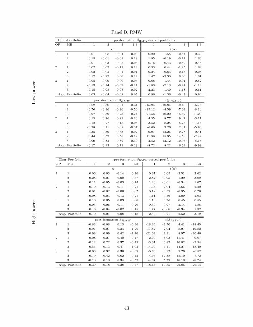
Panel B: RMWL

owp

ower

Char-Portfolio pre-formation βRMW-sorted portfolios

OP ME 1 2 3 1-3 1 2 3 1-3

α t(α)

1 1 -0.01 0.08 -0.04 0.03 -0.20 1.55 -0.64 0.30

2 0.19 -0.01 -0.01 0.19 1.95 -0.19 -0.11 1.66

3 0.01 -0.03 -0.05 0.06 0.16 -0.43 -0.59 0.48

2 1 0.02 0.02 -0.11 0.14 0.33 0.44 -1.95 1.68

2 0.02 -0.05 0.01 0.01 0.24 -0.83 0.13 0.08

3 0.12 -0.22 0.00 0.12 1.47 -3.30 0.00 1.01

3 1 -0.05 0.09 0.00 -0.05 -0.68 1.44 0.01 -0.52

2 -0.13 -0.14 -0.02 -0.11 -1.83 -2.18 -0.24 -1.18

3 0.15 -0.08 0.08 0.07 2.23 -1.40 1.18 0.61

Avg. Portfolio 0.03 -0.04 -0.02 0.05 0.96 -1.36 -0.47 0.94

post-formation βRMW t(βRMW )

1 1 -0.62 -0.30 -0.31 -0.31 -15.94 -10.84 -9.40 -6.78

2 -0.76 -0.16 -0.26 -0.50 -15.12 -4.59 -7.02 -8.14

3 -0.97 -0.39 -0.23 -0.74 -21.56 -10.20 -5.62 -11.23

2 1 0.15 0.26 0.29 -0.13 4.55 8.77 9.41 -3.17

2 0.12 0.27 0.18 -0.05 3.52 8.25 5.23 -1.16

3 -0.28 0.11 0.09 -0.37 -6.60 3.26 2.31 -5.96

3 1 0.35 0.39 0.33 0.02 9.07 12.26 9.28 0.41

2 0.44 0.52 0.56 -0.12 11.99 15.95 14.58 -2.49

3 0.09 0.35 0.39 -0.30 2.52 12.12 10.96 -5.15

Avg. Portfolio -0.17 0.12 0.11 -0.28 -8.72 8.22 6.62 -9.98

Hig

hp

ower

Char-Portfolio pre-formation βRMW-sorted portfolios

OP ME 1 2 3 1-3 1 2 3 1-3

α t(α)

1 1 0.06 0.03 -0.14 0.20 0.67 0.65 -2.51 2.02

2 0.28 -0.07 -0.09 0.37 2.87 -0.95 -1.29 3.09

3 0.11 -0.05 -0.03 0.14 1.23 -0.61 -0.34 1.07

2 1 0.10 0.13 -0.11 0.21 1.36 2.04 -1.66 2.20

2 0.01 -0.02 -0.06 0.07 0.12 -0.39 -0.95 0.76

3 0.08 -0.03 -0.13 0.21 1.11 -0.56 -2.09 2.03

3 1 0.10 0.05 0.03 0.06 1.16 0.76 0.45 0.55

2 0.03 -0.06 -0.17 0.20 0.39 -0.97 -2.14 1.88

3 0.13 -0.04 -0.02 0.15 1.77 -0.68 -0.34 1.32

Avg. Portfolio 0.10 -0.01 -0.08 0.18 2.49 -0.21 -2.52 3.19

post-formation βRMW t(βRMW )

1 1 -0.83 -0.08 0.13 -0.96 -18.60 -2.70 4.41 -18.45

2 -0.91 0.07 0.34 -1.26 -17.87 2.04 8.97 -19.82

3 -0.98 0.09 0.42 -1.40 -21.02 2.11 8.97 -20.46

2 1 -0.08 0.27 0.40 -0.47 -2.09 8.03 11.41 -9.67

2 -0.12 0.22 0.37 -0.49 -3.07 6.82 10.82 -9.94

3 -0.55 0.13 0.47 -1.02 -14.09 4.11 14.27 -18.40

3 1 -0.03 0.32 0.36 -0.39 -0.66 8.92 9.20 -6.52

2 0.19 0.42 0.62 -0.42 4.93 12.38 15.10 -7.72

3 -0.18 0.18 0.34 -0.52 -4.87 5.79 10.18 -8.74

Avg. Portfolio -0.39 0.18 0.38 -0.77 -18.66 10.85 22.85 -26.14

43

Panel C: CMAL

owp

ower

Char-Portfolio pre-formation βCMA-sorted portfolios

INV ME 1 2 3 1-3 1 2 3 1-3

α t(α)

1 1 0.07 0.09 0.10 -0.04 0.93 1.89 1.40 -0.40

2 -0.05 0.02 -0.07 0.02 -0.68 0.34 -0.94 0.22

3 -0.06 -0.03 -0.14 0.08 -0.74 -0.40 -1.77 0.63

2 1 0.12 0.03 0.17 -0.05 1.89 0.51 2.54 -0.57

2 0.07 -0.05 0.16 -0.09 1.10 -0.90 2.18 -0.94

3 0.03 -0.10 -0.01 0.04 0.42 -1.72 -0.19 0.40

3 1 -0.16 -0.16 -0.11 -0.05 -2.28 -2.86 -1.76 -0.58

2 -0.11 -0.07 0.10 -0.21 -1.40 -1.19 1.38 -1.94

3 0.23 -0.07 0.11 0.13 2.70 -1.01 1.56 0.97

Avg. Portfolio 0.01 -0.04 0.03 -0.02 0.40 -1.27 0.98 -0.32

post-formation βCMA t(βCMA)

1 1 0.17 0.31 0.57 -0.40 3.13 8.30 10.37 -5.92

2 0.19 0.44 0.74 -0.55 3.40 9.02 12.53 -6.96

3 0.23 0.63 1.18 -0.95 3.94 11.97 20.31 -10.19

2 1 -0.08 0.13 0.28 -0.36 -1.75 2.86 5.54 -5.37

2 -0.06 0.08 0.16 -0.21 -1.11 1.82 2.79 -2.99

3 -0.12 0.09 0.46 -0.58 -2.15 2.03 9.53 -7.22

3 1 -0.54 -0.17 -0.01 -0.53 -9.93 -4.16 -0.16 -7.53

2 -0.74 -0.17 0.08 -0.82 -11.93 -3.77 1.42 -9.93

3 -0.89 -0.28 0.07 -0.96 -13.57 -5.24 1.45 -9.69

Avg. Portfolio -0.20 0.12 0.39 -0.60 -7.19 5.28 14.98 -13.33

Hig

hp

ower

Char-Portfolio pre-formation βCMA-sorted portfolios

INV ME 1 2 3 1-3 1 2 3 1-3

α t(α)

1 1 0.05 0.13 0.15 -0.10 0.67 2.44 1.82 -0.97

2 0.19 0.09 -0.14 0.33 2.41 1.29 -1.70 2.98

3 0.29 -0.02 -0.12 0.41 2.80 -0.25 -1.54 2.94

2 1 0.08 0.14 0.05 0.03 1.23 2.11 0.72 0.32

2 0.14 0.03 -0.10 0.24 1.94 0.56 -1.33 2.30

3 0.12 -0.14 -0.09 0.21 1.55 -2.10 -1.45 1.84

3 1 -0.20 -0.07 -0.14 -0.06 -2.59 -1.11 -1.98 -0.56

2 -0.04 -0.06 -0.05 0.01 -0.46 -0.79 -0.59 0.06

3 0.39 -0.13 -0.13 0.52 4.64 -1.97 -1.66 3.90

Avg. Portfolio 0.11 -0.00 -0.06 0.18 2.77 -0.09 -1.68 2.69

post-formation βCMA t(βCMA)

1 1 -0.18 0.09 0.53 -0.70 -3.40 2.19 8.52 -8.75

2 -0.49 0.24 0.59 -1.08 -8.38 4.48 9.55 -13.10

3 -0.67 0.01 0.72 -1.40 -8.63 0.23 12.22 -13.27

2 1 -0.18 0.18 0.40 -0.58 -3.56 3.73 7.45 -7.73

2 -0.36 0.19 0.71 -1.07 -6.69 4.08 12.25 -13.51

3 -0.66 0.20 0.86 -1.52 -11.17 3.96 18.24 -17.53

3 1 -0.47 0.03 0.18 -0.65 -8.01 0.64 3.34 -7.89

2 -0.80 -0.04 0.41 -1.21 -12.63 -0.75 7.06 -14.08

3 -0.99 0.15 0.61 -1.60 -15.64 3.10 10.47 -15.97

Avg. Portfolio -0.53 0.12 0.56 -1.09 -17.38 4.40 19.76 -22.11

44

Table 5: Results of time-series regressions on characteristics-balanced hedge-portfolios.Stocks are first sorted based on size and one of book-to-market, profitability or investment into 3x3 portfolios.Conditional on those sorts, they are subsequently sorted into 3 portfolios based on the respective loading,i.e., on HML, RMW or CMA. For Mkt-RF and SMB we use the prior sort on size and book-to-market. The”hedge-portfolio” then goes long the low loading and short the high loading portfolios. On the bottom, weform combination-portfolios that put equal weight on three (HML, RMW, CMA), four (HML, RMW, CMA,Mkt-RF) or five (HML, RMW, CMA, Mkt-RF, SMB) hedge-portfolios portfolios. Monthly returns of theseportfolios are then regressed on the 5 Fama and French factors in the sample period from 1963/07 - 2017/12.In Panel A we use the low power and in Panel B we use the high power methodology.

Panel A: Low power

Hedge-Portfolio Avg. α βMkt−RF βSMB βHML βRMW βCMA R2

hMktRF -0.07 0.08 -0.27 -0.16 0.07 0.08 -0.07 0.49

(-0.82) (1.37) (-17.43) (-7.68) (2.47) (2.49) (-1.40)

hSMB -0.11 -0.02 -0.12 -0.34 0.06 0.05 0.13 0.56

(-1.39) (-0.31) (-9.46) (-18.55) (2.57) (1.86) (3.23)

hHML -0.02 0.09 -0.02 -0.02 -0.49 -0.04 0.41 0.35

(-0.21) (1.43) (-1.52) (-1.09) (-17.02) (-1.27) (8.76)

hRMW -0.07 0.05 0.05 -0.05 -0.14 -0.28 -0.01 0.29

(-1.11) (0.96) (3.81) (-2.96) (-5.63) (-10.04) (-0.31)

hCMA -0.09 -0.03 -0.01 -0.01 0.26 -0.03 -0.60 0.25

(-1.38) (-0.44) (-0.67) (-0.56) (9.65) (-1.02) (-13.41)

EW3 -0.06 0.04 0.01 -0.03 -0.12 -0.12 -0.07 0.37

HML,RMW,CMA (-1.72) (1.37) (0.83) (-3.11) (-9.50) (-8.10) (-3.17)

EW4 -0.06 0.05 -0.06 -0.06 -0.07 -0.07 -0.07 0.25

EW3+MktRF (-1.94) (1.77) (-8.99) (-6.53) (-5.65) (-4.61) (-3.11)

EW5 -0.07 0.04 -0.06 -0.10 -0.06 -0.06 -0.04 0.29

EW4+SMB (-2.12) (1.40) (-9.02) (-10.30) (-4.76) (-4.00) (-1.82)

Panel B: High power

Hedge-Portfolio Avg. α βMkt−RF βSMB βHML βRMW βCMA R2

hMktRF -0.09 0.21 -0.42 -0.38 -0.05 0.12 0.05 0.64

(-0.70) (2.69) (-21.96) (-14.30) (-1.29) (3.00) (0.84)

hSMB -0.19 -0.03 -0.18 -0.56 0.02 0.15 0.14 0.73

(-1.85) (-0.59) (-12.55) (-28.48) (0.93) (4.97) (3.19)

hHML -0.08 0.20 -0.01 0.08 -0.94 -0.24 0.44 0.76

(-0.70) (3.50) (-0.90) (4.10) (-35.96) (-8.15) (10.42)

hRMW -0.13 0.18 0.04 -0.06 -0.27 -0.77 -0.04 0.67

(-1.43) (3.27) (3.08) (-3.25) (-10.44) (-26.31) (-0.99)

hCMA -0.02 0.17 -0.02 -0.03 0.31 -0.11 -1.09 0.49

(-0.27) (2.60) (-1.07) (-1.49) (10.18) (-3.26) (-22.30)

EW3 -0.08 0.18 0.00 -0.01 -0.30 -0.37 -0.23 0.78

HML,RMW,CMA (-1.20) (5.68) (0.54) (-0.48) (-20.18) (-22.13) (-9.44)

EW4 -0.08 0.19 -0.10 -0.10 -0.24 -0.25 -0.16 0.64

EW3+MktRF (-1.64) (6.18) (-13.43) (-9.41) (-16.77) (-15.60) (-6.93)

EW5 -0.09 0.16 -0.10 -0.15 -0.21 -0.21 -0.13 0.61

EW4+SMB (-2.08) (5.19) (-13.03) (-14.55) (-14.99) (-13.36) (-5.61)

45

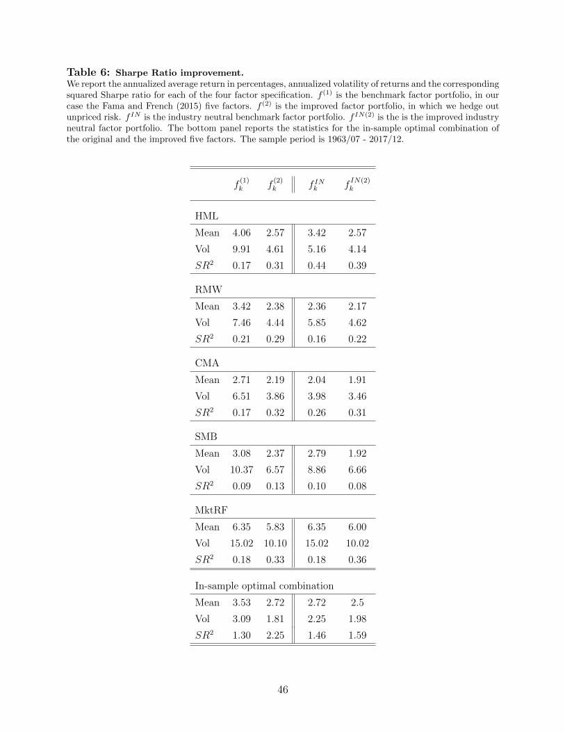
Table 6: Sharpe Ratio improvement.We report the annualized average return in percentages, annualized volatility of returns and the correspondingsquared Sharpe ratio for each of the four factor specification. f (1) is the benchmark factor portfolio, in ourcase the Fama and French (2015) five factors. f (2) is the improved factor portfolio, in which we hedge outunpriced risk. f IN is the industry neutral benchmark factor portfolio. f IN(2) is the is the improved industryneutral factor portfolio. The bottom panel reports the statistics for the in-sample optimal combination ofthe original and the improved five factors. The sample period is 1963/07 - 2017/12.

f(1)k f

(2)k f INk f

IN(2)k

HML

Mean 4.06 2.57 3.42 2.57

Vol 9.91 4.61 5.16 4.14

SR2 0.17 0.31 0.44 0.39

RMW

Mean 3.42 2.38 2.36 2.17

Vol 7.46 4.44 5.85 4.62

SR2 0.21 0.29 0.16 0.22

CMA

Mean 2.71 2.19 2.04 1.91

Vol 6.51 3.86 3.98 3.46

SR2 0.17 0.32 0.26 0.31

SMB

Mean 3.08 2.37 2.79 1.92

Vol 10.37 6.57 8.86 6.66

SR2 0.09 0.13 0.10 0.08

MktRF

Mean 6.35 5.83 6.35 6.00

Vol 15.02 10.10 15.02 10.02

SR2 0.18 0.33 0.18 0.36

In-sample optimal combination

Mean 3.53 2.72 2.72 2.5

Vol 3.09 1.81 2.25 1.98

SR2 1.30 2.25 1.46 1.59

46

Table 7: Ex-post optimal Markowitz weights.We report the weights on each of the five factors from a full-sample ex-post Markowitz optimization. Thefirst column reports results for the original five factors, and the second column for the improved versions ofthese five factors. The sample period is 1963/07 - 2017/12.

f(1)k f

(2)k

CMA 0.39 0.31

HML -0.01 0.12

MktRF 0.15 0.11

RMW 0.36 0.33

SMB 0.12 0.12

Table 8: Spanning tests for HML.We regress the original HML (first 2 columns) as well as the improved version of HML (columns 3 and 4)on the remaining four original and improved factors. The sample period is 1963/07 - 2017/12.

Portfolio HML(1) HML(1) HML(2) HML(2)

α -0.02 (-0.26) 0.11 (0.94) 0.17 (3.34) 0.11 (2.51)

βMktRF (1) 0.01 (0.44) -0.01 (-1.01)

βSMB(1) 0.03 (1.10) 0.04 (2.47)

βRMW (1) 0.36 (8.49) -0.05 (-1.96)

βCMA(1) 1.09 (22.97) 0.24 (8.64)

βMktRF (2) 0.06 (1.50) 0.01 (0.47)

βSMB(2) 0.11 (1.82) 0.06 (2.66)

βRMW (2) 0.23 (2.40) -0.13 (-3.55)

βCMA(2) 0.71 (6.31) 0.61 (14.14)

R2 0.49 0.06 0.16 0.36

47