The Classical Electron Problem

Tepper L. Gill1,2,4, W. W. Zachary1,5 and J.Lindesay3

1Department of Electrical Engineering2Department of Mathematics

3Department of PhysicsHoward University,Washington, DC 20059

E-mail tgill@howard.edu4Department of PhysicsUniversity of Michigan

Ann Arbor, Mich. 481095Department of Mathematics and StatisticsUniversity of Maryland University College

College Park, Maryland 20742E-mail: wwzachary@earthlink.net

Abstract

In this paper, we construct a parallel image of the conventional Maxwell theory by replac-ing the observer-time by the proper-time of the source. This formulation is mathematically,but not physically, equivalent to the conventional form. The change induces a new sym-metry group which is distinct from, but closely related to the Lorentz group, and fixesthe clock of the source for all observers. The new wave equation contains an additionalterm (dissipative), which arises instantaneously with acceleration. This shows that theorigin of radiation reaction is not the action of a “charge” on itself but arises from inertialresistance to changes in motion. This dissipative term is equivalent to an effective massso that classical radiation has both a massless and a massive part. Hence, at the locallevel the theory is one of particles and fields but there is no self-energy divergence (norany of the other problems). We also show that, for any closed system of particles, there isa global inertial frame and unique (invariant) global proper-time (for each observer) fromwhich to observe the system. This global clock is intrinsically related to the proper clocksof the individual particles and provides a unique definition of simultaneity for all eventsassociated with the system. We suggest that this clock is the historical clock of Horwitz,Piron, and Fanchi. At this level, the theory is of the action-at-a-distance type and theabsorption hypothesis of Wheeler and Feynman follows from global conservation of energy.

PACS classification codes: 03.30.+,03.50.DeKeywords: generalized Maxwell theory, special relativity, radiation reaction

1

1.0 Introduction

It was 1865 when James Clark Maxwell published his theory of electrodynamics. The slow

but steady progress made by our understanding and use of mechanics and thermodynamics

was given a major boost by Maxwell’s theory made practical. For example, starting from

1866, a continuous communications link has existed between Europe and the US ( due in

no small part to the efforts of Lord Kelvin). By 1883, Edison had a workable light bulb,

while Bell invented the telephone in 1886. The radio waves predicted by Maxwell were

discovered by Hertz in 1887, and electricity, producing new inventions weekly, was well on

the way to providing what we now consider normal.

In the intervening 41 years between Maxwell and the introduction of the special theory

of relativity in 1905, a scientific and technological revolution had taken firm roots. Indeed,

it has been suggested by Feynman1 that, “ From the long view of the history of mankind-

seen from, say ten thousand years... there can be little doubt that the most significant event

of the 19th century will be judged as Maxwell’s discovery of the laws of electrodynamics.”

When the founding fathers, Lorentz, Poincare, Einstein, and their contemporaries

began to study the issues associated with the foundations of electrodynamics; they had a

number of options open to them in addressing the fact that the Newtonian theory and the

Maxwell theory were invariant under different transformation groups: (see Jackson2 )

1. Both theories are incorrect and a correct theory is yet to be found.

2. The “proper” Maxwell theory will be invariant under the Galilean group.

3. The “proper” Newtonian theory will be invariant under the Lorentz group.

4. The assumption of an ether for electromagnetic propagation is correct so that

2

Galilean relativity applies to mechanics while electromagnetism has a pre-

ferred reference frame.

At the time, it was unthinkable that the Maxwell theory had any serious flaws.

Lorentz3,4 had recently shown that all of the macroscopic phenomena of electrodynam-

ics and optics could be accounted for based on an analysis of the microscopic behavior of

electrons and ions.

Einstein5 rejected the fourth possibility and, as noted by Spencer and Shama6, was

the “ first scientist with the foresight to realize that a formal postulate on the velocity

of light was necessary.” He proposed that all physical theories should satisfy the (now

well-known) postulates of special relativity:

1. The physical laws of nature and the results of all experiments are independent

of the particular inertial frame of the observer (in which the experiment is

performed).

2. The speed of light in empty space is constant and is independent of the motion

of the source or receiver.

The first postulate abandons the notion of an absolute space , while the second abandons

absolute time. In a later paper, Einstein7 modified the second postulate to make it explicit

that he always referred to observers in inertial frames:

2′. The speed of light in empty space is constant and independent of the

motion of the source or receiver in any inertial frame.

Einstein formulated his theory in the usual three-dimensional notation, making a

3

distinction between time and space. It was noted by Poincare8 that the transformations of

Lorentz could be treated as rotations if time is made an imaginary coordinate. Poincare

had also introduced the metric now attributed to Minkowski9.

Although Poincare discovered the proper-time, it was Minkowski who recognized its

importance in physical theory and showed that it is the only unique variable associated

with the source and available to all observers. Motivated by philosophical concerns, he

further proposed that space and time should not be treated separately, but should be

unified in the now well-known fashion leading to Minkowski space. Given the tremendous

impact of the then-recent work in geometry on science, it was natural for him to think

along these lines. Once he accepted this approach, it was also natural to assume that the

proper-time of the source be used to parameterize the motion, acting as the metric for the

underlying geometrization of the special theory of relativity, thus implicitly requiring that

another postulate be added:

3. The correct implementation of the first two postulates requires that time be

treated as a fourth coordinate, and the relationship between components so

constrained to satisfy the natural invariance induced by the Lorentz group of

electrodynamics, (Minkowski space).

The four-geometry postulate was very popular at the time and was embraced by many;

but other important physical thinkers, including Einstein, Lorentz, Poincare, and Ritz,

regarded it as a mathematical abstraction lacking physical content and maintained that

space and time have distinct physical properties. Although Einstein demurred, the feeling

among many of the leading physicists at that time was that an alternative implementation

4

should be possible which preserves some remnant of an absolute time variable (true time),

while still allowing for the constancy of the speed of light. It was noted by Whittaker10

that a few weeks before he died, Lorentz is reported to have maintained his belief in the

existence of this “true time”. Dresden11 reports that “· · · He retained his beliefs in a

Euclidean, Newtonian space time, and in absolute simultaneity · · ·.”

1.1 Perspective

The general focus on, and excitement about, the four-geometry left little room for serious

alternative investigations (separated from philosophical debates). This is unfortunate since

the diversion is part of the reason that the physical foundations of classical electrodynam-

ics did not receive the early intense investigation accorded mechanics. Possibly because

of the apparent completeness of the special theory, interest in statistical mechanics, quan-

tum theory, and the problem of accelerated motion (the general theory), Einstein was

preoccupied with these other important areas. On the other hand, the physics community

lost three important thinkers on the subject by 1912. Ritz died in 1908, Minkowski died

(shortly after his paper appeared) in 1909, and Poincare died in 1912. The First World

War began in 1914 and within four years decimated a whole generation. Furthermore, by

1913 interests had already shifted from electrodynamics to the new quantum theory. The

longer this investigation into classical electrodynamics was delayed, the more Minkowski’s

approach became embedded in the culture of physics, permeating the foundations for all

future theories. By the time problems in attempts to merge the special theory of relativity

with quantum theory forced researchers to take a new look at the foundations of classical

electrodynamics, the Minkowski approach to the implementation of the special theory was

5

considered almost sacred.

We are now taking our first steps into the twenty first century, one hundred and forty-

five years later. Electromagnetism is now in the hands of the engineers, mathematicians,

and philosophers, and much of it is not considered mainstream physics. For those who

learned physics in the sixties and seventies, “electrodynamics seems as old as mechanics”.

The continued success of quantum mechanics and the “apparent” successes of quantum

electrodynamics and the standard model has made the subject passe. Today, students

study the subject as an introduction to the special theory, preparation for advanced quan-

tum theory, and as a simple example of a gauge theory. From this perspective, there is

no real reason to believe that the first possibility should be rejected out of hand (i.e., that

both the Newtonian and Maxwell theories could in some way be incorrect). Such a possi-

bility is even more likely in light of the fact that the problems facing the early workers are

still with us in one form or another. Furthermore, additional problems have arisen from

both theory and experiment.

1.2 Problems

Newtonian Mechanics

Once it was accepted that the ”proper” Newtonian theory should be invariant under the

Lorentz group, work on this problem was generally ignored until after World War Two

when everyone realized that the quantum theory did not solve the problems left open by the

classical theory. In particular, it was first noticed that (at the classical level) Minkowski’s

approach only works (as expected) in the one-particle case. It was 1948 when Pryce12

showed that the canonical center-of-mass is not the three-vector part of a four-vector.

6

This variable is required for any “natural” relativistic many-particle theory. Virtually all

research since then has focused on attempts to avoid this problem while maintaining use

of the proper-time of the observer as the fourth coordinate for Minkowski geometry.

In order to provide a simple approach to the problem encountered by Pryce, let us

consider two inertial observers X and X ′ with the same orientation. Assume that the

(proper) clocks of X and X ′ both begin when their origins coincide and X ′ is moving with

uniform velocity v as seen by X. Let two particles, each the source of an electromagnetic

field, move with velocities wi (i = 1, 2), as seen by X, and w′i (i = 1, 2), as seen by X ′, so

that:

x′i = xi − γ(v)vt + (γ(v) − 1)(xi · v/ ‖v‖2)v, (1.1a)

xi = x′i + γ(v)vt′ + (γ(v) − 1)

(x′

i · v/ ‖v‖2)v, (1.1b)

with γ(v) = 1/[1 − (v/c)2

]1/2

, represent the spacial Lorentz transformations between the

corresponding observers. Thus, there is clearly no problem in requiring that the positions

transform as expected. However, when we try to transform the clocks, we see the problem

at once since we must have, for example,

t′ = γ(v)(t − x1 · v/c2

), t′ = γ(v)

(t − x2 · v/c2

). (1.2a)

This is clearly impossible except under very special conditions on all other observers.

Furthermore, if we write down the center-of-mass position X and require that it transform

as above, we add another (impossible) constraint on the clock of any other observer. Pryce’s

approach is more abstract (and complicated), but leads to the same result.

In his 1949 paper, Dirac13 observed that we must choose a particular realization of

the Poincare algebra in order to identify the appropriate variables for theory formulation.

7

He showed that there are three possible choices of distinct three-dimensional hypersurfaces

that are invariant under subgroups of the Poincare group and intersect every particle world-

line once; the instant form, the point form, and the front form. (It was later shown by

Leutwyler and Stern14 that there are five choices. However, the other two are not especially

interesting.) The instant form is best known. It is based on normal time-evolution and uses

spacelike hyperplanes in Minkowski space; the point form is based on mass hyperboloids;

while the front form is based on null hyperplanes.

Following Dirac’s work, Bakamjian and Thomas15 showed that one can construct a

quantizable many-particle theory that satisfies the first two postulates of Einstein. How-

ever, they suggested that when interaction is introduced, their approach would not permit

both a global theory and provide an invariant particle world-line description (satisfy the

third postulate). This conjecture was generalized and later proved by Currie et al16 to the

effect that the requirements of Hamiltonian formulation, (canonical) independent-particle

variables, and relativistic covariance (i.e the canonical positions transform as geomet-

ric coordinates), are only compatible with noninteracting particles (The No-Interaction

Theorem). There are many references on the subject, but the book by Sudarshan and

Mukunda17 gives a comprehensive review of the problems and attempts to solve them (up

to 1974). All attempts have ended in failure for one or more reasons which usually include

the inability to quantize.

The No-Interaction Theorem led many to suspend the requirement that canonical po-

sitions transform as geometric coordinates and to focus on the construction of the “correct

many-particle representation for the Poincare algebra”. However, a very important (but

8

not well-known) theorem was proved by Fong and Sucher18 in 1964 for the quantum case,

and by Peres19 in 1971 for the classical case:

Theorem 1.0 (Fong-Sucher-Peres) Suppose that no restriction is put on the transforma-

tion law of the canonical variables of a many-particle system. Then given any Hamiltonian

H, total momentun P, and angular momentum J satisfying:

dH/dt = 0, [H, Pm] = 0, [H, Jm] = 0,[Pm, Pn] = 0, [Jm, Pn] = εmnsPs, [Jm, Jn] = εmnsJs,

it is always possible to find a boost generator L so that the full set of commutation relations

of the Poincare algebra for the inhomogeneous Lorentz group will be satisfied.

In order to underscore the importance of this theorem, Peres showed explicitly how to

construct a “clearly” nonrelativistic Hamiltonian and appropriate boost generator (along

with canonical center-of-mass, total momentum, and angular momentum). Thus, this

theorem implies that a relativistic classical (or quantum) many-particle theory requires

something else besides the commutation relations for the inhomogeneous Lorentz group.

On the other hand, this is the only requirement imposed on us by Maxwell’s equations!

It follows that, contrary to common belief, our historical (intellectual) state of affairs is

not dictated by the Maxwell theory. We conclude that the Minkowski postulate imposes

an additional condition on the special theory (not required by Maxwell’s equations), but

we are still unable to correctly account for Newtonian mechanics (after almost a hundred

years). Those willing to dismiss the issue as arcane should be aware that the same problem

also exists for the general theory. Thus, the major problem facing us in the twenty first

century is to construct a quantizable classical theory which satisfies the first two postulates

of Einstein in some reasonable form and includes Newtonian Mechanics.

9

Interpretation

There are interpretation problems with the Minkowski approach that are not well-known.

First, it should be noted that the conventional use of the words coordinate time tends

to obscure the fact that this is the proper-time of the observer. This makes physical

interpretation complicated and strange because one is required to refer back to the proper-

time of the source (or the postulated clock of a co-moving observer) in order to acquire

a complete interpretation and analysis of experiments. Thus, the “parameter” (used to

define the four-geometry) must also be viewed as a physically real measurable quantity

when the theory is used for experimental analysis. At the classical level this asymmetrical

relationship may be vexing, but it is not contradictory. However, at the quantum level

this same problem becomes more fundamental. At this level, the observer proper-time is a

c-number that transforms to an operator under the Lorentz group, while the proper-time

of the source is an operator that remains invariant (see Wigner20).

Radiation Reaction and the Lorentz-Dirac Equation

The problems associated with the radiation of accelerated charged particles, and those

of the Lorentz-Dirac equation are old and well-known. Two books that have contributed

to a clearer understanding of these basic problems are those of Rohrlich21 and Parrott22.

Rohrlich provides a comprehensive study of the classical theory up to 1965, which includes

a nice review of the history. (Those unaware of the continuing effort to solve the classical

electron problem should also see Rohrlich23.) Parrott’s book is both clear and insightful.

(His chapter on the Lorentz-Dirac equation is unbiased, well done, and should be required

reading for any serious student of the subject.) The classics, Panofsky and Phillips24, and

10

Jackson2 are also important sources of insight and history. The elementary (but correct)

account by Feynman1 in volume II of his famous lecture series has done much to educate

those with little or no concern with the foundations.

The radiation of accelerated charged particles is known to occur instantaneously with

acceleration and its nature has been the object of much speculation (see Wheeler and

Feynman25). The great success of Lorentz in using the Maxwell (field) theory, along

with his aether, to show that all of the macroscopic electrodynamics and optics could be

derived from a microscopic analysis has done much to foster our faith in the correctness

of the theory. This success carried with it our first introduction to the divergences of a

field theory. He found that the energy density and the field momentum for each particle

diverges unless the particle has a finite radius. In addition, the derived (Lorentz) force

law did not provide the appropriate dissipation to account for the observed radiation. It

was also known that the electromagnetic mass defined by the electrostatic energy divided

by c2 and that defined via the electomagnetic momentum did not agree, giving the well

known 4/3’s problem (see Schwinger26).

These problems led to the study of various finite-size models for charged particles

and, in turn, forced serious consideration of the action of one part of a charge on itself

(self-energy) and also required the introduction of extra forces to hold the particle together

(Poincare stresses).

The appearance of the classical divergence difficulties in the quantized theory (along

with a few new ones) led many to hope that the successful construction of a consistent clas-

sical theory would help to solve the corresponding problems in quantum electrodynamics.

11

For this reason, many attempts were made to formulate such a theory. The most well-

known early attempts are due to Born and Infield27, Dirac28, Bopp29, and Wheeler and

Feynman25. (Less well-known other attempts are due to Rosen30, Podolsky and Schwed31,

and Feynman32.) Each ran into problems with quantization and are a part of the history.

However, the point particle reduction theory of Dirac and the Wheeler-Feynman approach

have special importance.

The use of particles of finite radius causes serious problems with Lorentz invariance,

so a major advance was made when Dirac constructed a point particle reduction theory

for the Lorentz model. To do this, he used Maxwell’s equations to find the retarded field

of the particle, assuming that at large distances the field only contains outgoing waves,

and then calculated the advanced field assuming that at large distances the field only

contains converging waves. He then defined half the difference between the retarded and

the advanced fields evaluated at the particle position, multiplied by the charge, as the force

of radiation reaction. This term was added to the Lorentz force to provide the appropriate

dissipation term (the Lorentz-Dirac equation). This provided the same dissipation term

obtained by Lorentz (in a nonrelativistic calculation), but was independent of the particle

radius. Thus, Dirac produced a point particle theory while all the other problems remained

unchanged, and this is essentially what we have today. It should also be noted that point

particles of finite mass imply infinite density. This was a real problem during Newton’s

time, but does not appear to cause problems today.

Wheeler and Feynman took a different ploy. They showed that we could use point

particles, obtain the same radiation reaction term as above, and eliminate the self-energy

12

divergence. Their approach assumes that the field which acts on a given particle arises

only from other particles (adjunct field). They used half the sum of the retarded and

the advanced fields, and assumed that there are sufficiently many particles in the system

to completely absorb all radiation given off from any one of them (absorption hypothe-

sis). The theory is of the action-at-a-distance type and also eliminates the divergences

associated with the energy and momentum densities. Unfortunately, the theory could not

be quantized, but this work made it clear that the action-at-a-distance and field theory

approaches are much closer than was generally expected. (Indeed, Wheeler and Feynman

argued that the two theories are complimentary views.)

The two best-known problems with the Lorentz-Dirac equation are runaway solutions

and preacceleration. The equation has solutions for a free particle (with no force) that can

self-accelerate off to infinity. It was conjectured that these solutions were eliminated by

the asymptotic condition proposed by Haag33. However, Parrott22 (pg. 196) notes that

the asymptotic condition is necessary to ensure conservation of energy-momentum, but

may not be sufficient to eliminate all strange solutions. Furthermore, the recent paper of

Parrott and Endres34 makes this conjecture doubtful. It has been recently shown by Low35

that this problem also shows up at the nonrelativistic quantum level. Things are better

for quantum electrodynamics (they don’t appear), but caution is required as the possible

existence of a Landau-like anomalous pole in the photon propagator or the electron-massive

photon forward scattering amplitude could produce the runaway effect.

The preacceleration problem arises because the equation is nonlocal in time. This

means that the particle can accelerate prior to the action of a force. The problem is

13

generally ignored with the observation that the natural time interval for this effect (say for

an electron) is of the order of 6.2 × 10−24 sec, so that no classical particle can enter from

a free state into interaction over such a small time interval.

These problems have existed for sometime now and no solution seems to be in sight.

It is clear that the first problem is based on the assumption that the dissipation should

be in the Lorentz force and, since this term is of third order in the position variable, the

difficulty follows. The second problem can be traced back to the use of advanced fields

which are necessary for the theory (Dirac and Wheeler and Feynman), and to get the

correct dissipation term.

Mach’s Principle and the 2.7 K MBR

Today, we know that a unique preferred frame of rest exists throughout the universe

and is available to all observers. This is the 2.7 K microwave background radiation

(MBR) which was discovered by Penzias and Wilson36 in 1965 using basic microwave

equipment (by today’s standards). This radiation is now known to be highly isotropic

with anisotropy limits set at 0.001%. Futhermore, direct measurements have been made

of the velocity of both our Solar System and Galaxy through this radiation (370 and

600 km/sec respectively, see Peebles37 ). One can only speculate as to what impact this

information would have had on the thinking of Einstein, Lorentz, Minkowski, Poincare,

Ritz and the many other investigators of the early 1900’s who were concerned with the

foundations of electrodynamics and mechanics. The importance of this discovery for the

foundations of electrodynamics in our view is that this frame is caused by radiation from

accelerated charged particles (independent of the various cosmological suggestions).

14

As noted by Peebles, the MBR does not violate the special theory. However, general

relativity predicts that at each point we can adjust our acceleration locally to find a freely

falling frame where the special theory holds. In this frame, all observers with constant

velocity are equivalent. Thus, according to the general theory we have an infinite family

of freely falling frames. Within this context, the Penzias and Wilson findings show that

there is a unique frame in which both the acceleration and velocity can be set equal to

zero at each point in the universe.

As suggested by Rohrlich21, “Mach’s principle was originally designed to ensure that

there is no difference between the rotation of the earth with repect to the fixed stars or the

fixed stars with respect to the earth.” It now appears that the fixed stars are not needed

and the earth really does rotate. Our concern with this principle is associated with the fact

that an accelerated charged particle experiences a damping force simultaneously with the

moment of acceleration (relative to any inertial frame). Thus, it appears that a charged

particle can be used to identify accelerating frames and raises the question: what is a

charged particle accelerating with respect to? Put another way, charged particles appear

to know when they experience a force. Furthermore, even if the force is constant, the

effect cannot be transformed away. This is a problem for any theory that seeks to unify

electromagnetism with gravity.

1.3 Purpose

Dirac41 was critical of the use of Minkowski geometry as fundamental. As late as 1963,

he noted that “...the picture with four-dimensional symmetry does not give us the whole

situation... Quantum theory has taught us that we must take a three-dimensional section

15

of what appears to our consciousness at one time (an observation), and relate it to another

three-dimensional section at another time.” In reviewing attempts to merge gravitation

with quantum theory, Dirac goes on to question the fundamental nature of the four-

dimensional requirement in physics and notes that, in some cases, physical descriptions

are simplified when one departs from it. The real question is: What do we replace it with

that solves the outstanding problems and has some contact with the physics we know?

A major part of our strong belief in the fundamental nature of the covariant Minkowski

approach to theory construction is based on the Feynman-Schwinger-Tomonaga formu-

lation of QED and their great computational success in accounting for the Lamb shift

and the anomalous magnetic moment. The correct history is at variance with this belief

(see Schweber38). It should first be noted that, using noncovariant methods, French and

Weisskopf39, and Kroll and Lamb40 were the first to get the correct results. The history

of the French and Weisskopf paper can be found in Schweber and is well worth reading.

Both Schwinger and Feynman initially got incorrect results using their covariant formula-

tion and only after the work of French and Weisskopf was circulated did they find their

mistakes. Later, Tomonaga got the correct results but used noncovariant methods in the

middle of the calculation (see Schweber38, pg. 270).

In attempting to solve the problems of the classical electron, almost every possible change

has been explored except the Minkowski four-geometry requirement. Our purpose in this

paper is to carefully study the mathematical and physical implications that arise when

we replace the observer proper-time by the source proper-time in Maxwell’s equations. In

order to see how this is possible, we first recall Minkowski’s definition of the proper-time

16

of a source:

dτ2 = dt2 − 1c2

dx2 = dt2[1 −

(wc

)2]

, w =dxdt

, (1.3a)

dτ2 = dt′2 − 1

c2dx′2 = dt2

[1 −

(w′

c

)2]

, w′ =dx′

dt′. (1.3b)

Minkowski was aware that dτ is not an exact one-form and this observation may have

affected his decision to restrict its use to being a parameter for the four-geometry. However,

there is an important physical reason why it is not an exact (mathematical) one-form.

Physically, a particle can traverse many different paths (in space) during any given τ

interval. This reflects the fact that the distance a particle can travel in a given time

interval depends on the forces acting on it. This implies that the clock of the source

carries physical information, and there is no a priori physical reason to believe that this

information is properly encoded when τ is used as a parameter. We rewrite (1.3) as

dt2 = dτ2 +1c2

dx2 = (dτ)2[1 +

(uc

)2]

, u =dxdτ

, (1.4a)

dt′2 = dτ2 +

1c2

dx′2 = (dτ)2[1 +

(u′

c

)2]

, u′ =dx′

dτ. (1.4b)

Thus, another possibility appears (which does give an exact one-form). In case we have

two or more particles, our new time transformations are replaced by (in the simplest case)

a′iτi = γ(v)[aiτi − xi · v/c2], (1.2b)

where τi is the proper-time of the i-th particle and ai and a′i are terms which depend only

on τi.

In Section 2 we construct the invariance group which fixes the proper-time of the

source in the single particle case and then explore some of the physical implications and

17

interpretations of this approach. At this level we see that the speed of particles may be

faster than the speed of light. The physical interpretation is that the mass and the mean

lifetime of unstable particles are now both constant, while the velocity computed using the

clock of the source replaces the velocity computed using the observer clock. Thus, as will

be seen, there is no contradiction with the second postulate, only a change in conventions.

The second postulate is shown to always hold for experiments conducted with the source

at rest in the frame of the observer, as is the case for the Michelson-Morley experiment.

In Section 3 we show explicitly that Maxwell’s equations have an equivalent repre-

sentation which fixes the proper-time of the source for all observers. We then prove that

this formulation is left covariant under the action of the proper-time group. Although

the fields have the same transformation properties as the conventional formulation, both

the current and charge densities transform differently. In particular, we prove that if the

charge density is at rest in any inertial frame then it is invariant (not just covariant) for

all observers. By example, even in the accelerating case when the proper velocity is 2c,

the relative velocity of our observers must be a subtantial fraction of c for them to detect

any difference in their measured properties of the charge distribution.

In this Section we also derive the corresponding wave equations and show that they

contain an additional dissipative term,which arises instantaneously with acceleration. By

a change of variables, we show that the dissipative term is equivalent to an effective mass

for electromagnetic radiation. We validate this interpretation by directly calculating the

energy radiated by an accelerated charge in the proper-time formulation. The radiation

formulas obtained are close in form but differ from those computed via the conventional

18

formulation, but agree in the low-velocity limit. In particular, the proper-time theory

predicts an additional term for the E-field which acts along the direction of motion (longi-

tudinal), proving the validity of our interpretation of the wave equation. This result means

that in the proper-time formulation, there is no need to to require that the charge act back

on itself in order to account for radiation reaction. When we couple this result with the

the invariance of the charge density, we are able to prove that the proper-time theory is

independent of the particle size, structure and geometry.

In Section 4 we derive the related versions of the optical Doppler effect and the aberra-

tion of wave vectors. These two phenomena are both well-known and ubiquitous. However,

the general forms are usually derived using Lorentz transformations2,42. Here, we derive

them from the proper-time theory, using the new invariance group. In addition to the

usual terms, we obtain new results because of the nonlocal frequency effects implied by

our theory. These effects play an important role in our derivation of the group velocity for

electromagnetic waves. Here we show that the group velocity is c only when measured in

the (rest) frame of the observer, but will not be c for any other observer moving relative

to that frame. The new value (in the simplest case) will be either c+v or c−v, depending

on the direction of the relative motion. However, as will be shown in Section 6, this effect

is in the noise for experiments conducted up to now because of theory interpretation.

In Section 5 we formulate a global interacting many-particle theory. With an eye to-

wards the quantum theory, we require that the change from observer proper-time to source

proper-time be canonical. This leads to the Hamiltonian which generates τ translations.

To accomplish this, we use a representation of the proper-time that is independent of the

19

number of particles. We derive our many-particle theory via the commutation relations

for the Poincare algebra. As a side benefit, we show that the global system has a (unique)

proper-time (avaliable for all observers). This clock provides a unique definition of simul-

taneity for all events associated with the system and is (shown to be) intrinsically related

to the proper-times of the particles (in the system). From these results, it follows that at

the local level, during interaction, the proper-time group is a nonlinear and nonlocal rep-

resentation of the Lorentz group. On the other hand, at the global level, the proper-time

group differs from the Lorentz group by a scale transformation. It follows from the work

in this Section and in Section 2 that the group representation space is Euclidean.

In Section 6 we explore the ramifications and implications of our formulation and

discuss some apparent disadvantages.

2.0 Proper-Time Transformations

In this section, we derive the transformations that fix the proper-time of the source for all

observers. If we set b2 = u2 + c2, then from (1.1) and (1.4) we have that

t = (1/c)

τ∫0

b(s)ds and t′ = (1/c)

τ∫0

b(s)′ds. (2.0)

It follows that t and t′ are nonlocal as functions of τ in the sense that their values depend

on the particular physical history (proper-time path) of the source. By the mean value

property for integrals, we can find a unique s(τ) for each τ , 0 < s(τ) < τ , such that

uτ = u(τ − s(τ)), and

t = (1/c)

τ∫0

b(s)ds = (bτ/c)τ, (2.1a)

20

t′ = (1/c)

τ∫0

b′(s)ds = (b′τ/c)τ. (2.1b)

It is clear that this property is observer-independent since

t′ = γ(v)(t − x · v/c2) ⇒ (b′τ/c)τ = γ(v)[(bτ/c)τ − (x · v/c2)]. (2.2)

With a fixed clock for all observers, we can now develop a theory in which only the spatial

coordinates are transformed. Using (2.2), the required transformations are

x′ = x − γ(v )(bτ/c)vτ + (γ(v ) − 1)(x · v/||v||2)v, (2.3a)

x = x′ + γ(v )(b′τ/c)vτ + (γ(v ) − 1)(x′ · v/||v||2)v. (2.3b)

From a physical point of view, (2.3) tells us (explicitly) that observers can only share

information about the past position of a given physical system. The above approach also

gives us the only (presently known) rational solution to the problem of distant simultaneity.

It is clear that all observers have the option of using their proper clocks with no hope of

agreeing on the time occurrence of any event associated with the source. On the other

hand, if each observer agrees to use the proper clock of the source, we see that they will

always agree on the time occurrence of any event associated with the source.

We now see that ai = (bi/c) and a′i = (b′i/c) in equation (1.2b). The unit for b and b′

is velocity so that physical interpretation is very important. It will arise naturally when

we represent Maxwell’s equations using the proper-time of the source. For now, we note

that they are related by

b′ = γ(v)[b − u · v

c

], b = γ(v)

[b′ +

u′ · vc

]. (2.4)

21

For any vector d, set

d† = d/γ(v) − (1 − γ(v))[v · d/(γ(v)v2)

]v. (2.5)

Then the full set of transformations between observers that fix the proper-time of the

source take the (almost) familiar form

x′ = γ(v)[x† − (v/c)bττ

], x = γ(v)

[x′† + (v/c)b′ττ

], (2.6)

u′ = γ(v)[u† − (v/c)b

], u = γ(v)

[u′† + (v/c)b′

], (2.7)

a′ = γ(v)a† − v [u · a/(bc)]

, a = γ(v)

a′† + v [u′ · a′/(b′c)]

, (2.8)

where a (a′) is the particle proper-(three) acceleration. The above transformations (along

with (2.4)) form the proper-time group. In this formulation, we now have only one clock

as an intrinsic part of the theory.

The above transformations are so close to Lorentz transformations that one might

wonder if any new physics is possible. Not only is there new physics, as will be seen later,

but just as importantly, there are new physical interpretations of old ideas. For example,

relativistic momentum increase is attributed to relativistic mass increase so that

p = mw, m = m0[1 − w2/c2]−1/2. (2.9a)

In the new interpretation,

p = m0u, u = w[1 − w2/c2]−1/2, (2.9b)

so there is no mass increase, the (proper) velocity increases. Thus, in particle experiments

the particle will have a fixed mass and decay constant, independent of its velocity. On the

22

other hand, the particle can have (proper) speeds larger than the speed of light since its

velocity is now interpreted to be dx/dτ . All cases where time dilation is discussed in the

standard approach are replaced by statements about u in the new approach.

Note that the relationship between u and w can be viewed as dual in the sense that

u = w[1 − w2/c2]−1/2, (2.10)

w = u[1 + u2/c2]−1/2. (2.11a)

This relationship was first derived by Schott43 in the famous 1915 paper in which he also

derived the well-known Schott term of classical electrodynamics. Dividing by c in (2.11a),

we get

wc

=ub. (2.11b)

It is easy to show that [1 + u2/c2]1/2 = [1 − w2

/c2]−1/2. Expanding both sides and using

(2.11b), we have

[1 + u2/c2]1/2 = 1 +

12

u2

c2− 1

8u4

c4+ · · · , (2.12)

[1 − w2/c2]−1/2 = 1 +

12

w2

c2+

38

w4

c4+ · · · , (2.13a)

[1 − w2/c2]−1/2 = [1 − u2

/b2]−1/2 = 1 +

12

u2

b2+

38

u4

b4+ · · · . (2.13b)

Thus, all three expressions agree in the low-velocity region. It follows that all the results

derived from the standard implementation of special relativity using w/c can also be con-

sistently derived using u/b. This result will be repeatedly exploited in this paper to provide

an alternative interpretation of much of classical electrodynamics. The real question that

arises is which of these definitions of velocity is appropriate in the construction of faithful

representations of physical reality. (see Section 6).

23

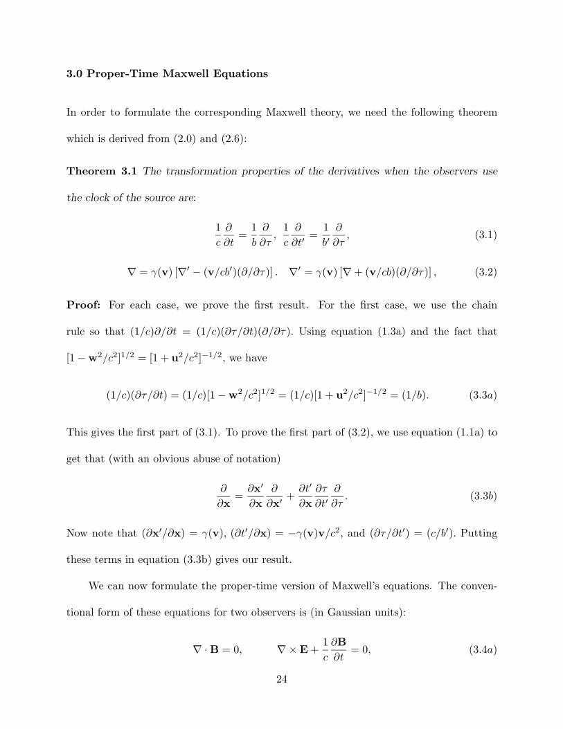
3.0 Proper-Time Maxwell Equations

In order to formulate the corresponding Maxwell theory, we need the following theorem

which is derived from (2.0) and (2.6):

Theorem 3.1 The transformation properties of the derivatives when the observers use

the clock of the source are:

1c

∂

∂t=

1b

∂

∂τ,

1c

∂

∂t′=

1b′

∂

∂τ, (3.1)

∇ = γ(v) [∇′ − (v/cb′)(∂/∂τ)] . ∇′ = γ(v) [∇ + (v/cb)(∂/∂τ)] , (3.2)

Proof: For each case, we prove the first result. For the first case, we use the chain

rule so that (1/c)∂/∂t = (1/c)(∂τ/∂t)(∂/∂τ). Using equation (1.3a) and the fact that

[1 − w2/c2]1/2 = [1 + u2/c2]−1/2, we have

(1/c)(∂τ/∂t) = (1/c)[1 − w2/c2]1/2 = (1/c)[1 + u2/c2]−1/2 = (1/b). (3.3a)

This gives the first part of (3.1). To prove the first part of (3.2), we use equation (1.1a) to

get that (with an obvious abuse of notation)

∂

∂x=

∂x′

∂x∂

∂x′ +∂t′

∂x∂τ

∂t′∂

∂τ. (3.3b)

Now note that (∂x′/∂x) = γ(v), (∂t′/∂x) = −γ(v)v/c2, and (∂τ/∂t′) = (c/b′). Putting

these terms in equation (3.3b) gives our result.

We can now formulate the proper-time version of Maxwell’s equations. The conven-

tional form of these equations for two observers is (in Gaussian units):

∇ · B = 0, ∇× E +1c

∂B∂t

= 0, (3.4a)

24

∇ · E = 4πρ, ∇× B =1c

[∂E∂t

+ 4πρw]

, (3.4b)

∇′ · B′ = 0, ∇′ × E′ +1c

∂B′

∂t′= 0, (3.5a)

∇′ · E′ = 4πρ′, ∇′ × B′ =1c

[∂E′

∂t′+ 4πρ′w′

]. (3.5b)

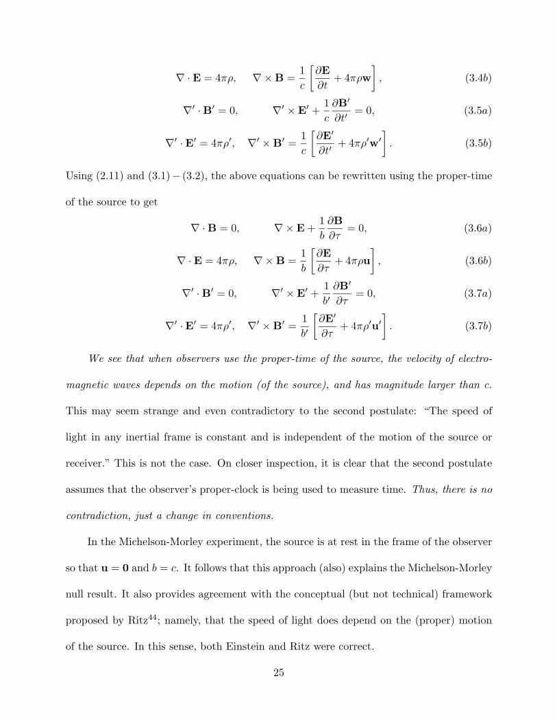
Using (2.11) and (3.1)− (3.2), the above equations can be rewritten using the proper-time

of the source to get

∇ · B = 0, ∇× E +1b

∂B∂τ

= 0, (3.6a)

∇ · E = 4πρ, ∇× B =1b

[∂E∂τ

+ 4πρu]

, (3.6b)

∇′ · B′ = 0, ∇′ × E′ +1b′

∂B′

∂τ= 0, (3.7a)

∇′ · E′ = 4πρ′, ∇′ × B′ =1b′

[∂E′

∂τ+ 4πρ′u′

]. (3.7b)

We see that when observers use the proper-time of the source, the velocity of electro-

magnetic waves depends on the motion (of the source), and has magnitude larger than c.

This may seem strange and even contradictory to the second postulate: “The speed of

light in any inertial frame is constant and is independent of the motion of the source or

receiver.” This is not the case. On closer inspection, it is clear that the second postulate

assumes that the observer’s proper-clock is being used to measure time. Thus, there is no

contradiction, just a change in conventions.

In the Michelson-Morley experiment, the source is at rest in the frame of the observer

so that u = 0 and b = c. It follows that this approach (also) explains the Michelson-Morley

null result. It also provides agreement with the conceptual (but not technical) framework

proposed by Ritz44; namely, that the speed of light does depend on the (proper) motion

of the source. In this sense, both Einstein and Ritz were correct.

25

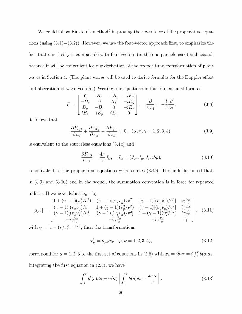
We could follow Einstein’s method5 in proving the covariance of the proper-time equa-

tions (using (3.1)−(3.2)). However, we use the four-vector approach first, to emphasize the

fact that our theory is compatible with four-vectors (in the one-particle case) and second,

because it will be convenient for our derivation of the proper-time transformation of plane

waves in Section 4. (The plane waves will be used to derive formulas for the Doppler effect

and aberration of wave vectors.) Writing our equations in four-dimensional form as

F =

0 Bz −By −iEx

−Bz 0 Bx −iEy

By −Bx 0 −iEz

iEx iEy iEz 0

,

∂

∂x4= − i

b

∂

∂τ, (3.8)

it follows that

∂Fαβ

∂xγ+

∂Fβγ

∂xα+

∂Fγα

∂xβ= 0, (α, β, γ = 1, 2, 3, 4), (3.9)

is equivalent to the sourceless equations (3.4a) and

∂Fαβ

∂xβ=

4π

bJα, Jα = (Jx, Jy, Jz, ibρ), (3.10)

is equivalent to the proper-time equations with sources (3.4b). It should be noted that,

in (3.9) and (3.10) and in the sequel, the summation convention is in force for repeated

indices. If we now define [aµν ] by

[aµν ] =

1 + (γ − 1)(v2x/v2) (γ − 1)[(vxvy)/v2] (γ − 1)[(vxvz)/v2] iγ

vx

c

(γ − 1)[(vxvy)/v2] 1 + (γ − 1)(v2y/v2) (γ − 1)[(vyvz)/v2] iγ

vy

c(γ − 1)[(vxvz)/v2] (γ − 1)[(vyvz)/v2] 1 + (γ − 1)(v2

z/v2) iγvz

c

−iγvx

c −iγvy

c −iγvz

c γ

, (3.11)

with γ = [1 − (v/c)2]−1/2; then the transformations

x′µ = aµνxν (µ, ν = 1, 2, 3, 4), (3.12)

correspond for µ = 1, 2, 3 to the first set of equations in (2.6) with x4 = ibττ = i∫ τ

0b(s)ds.

Integrating the first equation in (2.4), we have∫ τ

0

b′(s)ds = γ(v)[∫ τ

0

b(s)ds − x · vc

]. (3.13)

26

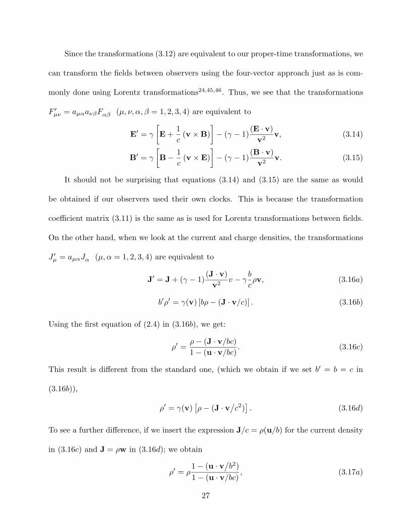
Since the transformations (3.12) are equivalent to our proper-time transformations, we

can transform the fields between observers using the four-vector approach just as is com-

monly done using Lorentz transformations24,45,46. Thus, we see that the transformations

F ′µν = aµαaνβFαβ (µ, ν, α, β = 1, 2, 3, 4) are equivalent to

E′ = γ

[E +

1c

(v × B)]− (γ − 1)

(E · v)v2

v, (3.14)

B′ = γ

[B − 1

c(v × E)

]− (γ − 1)

(B · v)v2

v. (3.15)

It should not be surprising that equations (3.14) and (3.15) are the same as would

be obtained if our observers used their own clocks. This is because the transformation

coefficient matrix (3.11) is the same as is used for Lorentz transformations between fields.

On the other hand, when we look at the current and charge densities, the transformations

J ′µ = aµαJα (µ, α = 1, 2, 3, 4) are equivalent to

J′ = J + (γ − 1)(J · v)

v2v − γ

b

cρv, (3.16a)

b′ρ′ = γ(v) [bρ − (J · v/c)] . (3.16b)

Using the first equation of (2.4) in (3.16b), we get:

ρ′ =ρ − (J · v/bc)1 − (u · v/bc)

. (3.16c)

This result is different from the standard one, (which we obtain if we set b′ = b = c in

(3.16b)),

ρ′ = γ(v)[ρ − (J · v

/c2)

]. (3.16d)

To see a further difference, if we insert the expression J/c = ρ(u/b) for the current density

in (3.16c) and J = ρw in (3.16d); we obtain

ρ′ = ρ1 − (u · v

/b2)

1 − (u · v/bc), (3.17a)

27

ρ′ = ργ(v)[1 − (w · v

/c2)

]. (3.17b)

In order to obtain a sense of the difference between ρ and ρ′, assume that

u = 2c ≈ u′, b =√

5c, ⇒ w = 2√5c ≈ c,⇒

ρ′ = ρ

[1 − 2v

5c

1 − 2v√5c

], & ρ = ρ′

[1 + 2v

5c

1 + 2v√5c

].

It follows that, unless the relative speed of our two observers is a substantial fraction

of c, they will decide that ρ = ρ′. In fact, we obtain the following remarkable result from

equation (3.17a):

Theorem 3.2 If the source is at rest in the X frame then ρ = ρ′ for all other observers.

Proof: The proof is easy, just note that if u = 0 in X then b = c and, from equation

(2.17a), ρ = ρ′. Since X ′ is arbitrary, the result is true for all observers.

The above theorem means that, in the proper-time formulation, a spherical charge

distribution at rest in any inertial frame will appear spherical to all other inertial ob-

servers. As will be shown in the next section, the radiation from an accelerated charged

particle appears as a dissipative term in the wave equations for the fields (i.e., neither

self-interaction or advanced fields are required). From these two results, we see that the

proper-time formulation is independent of particle size or structure.

3.1 Proper-Time Wave Equations

If in equations (3.6), we set

B = ∇× A, E = −1b

∂A∂τ

−∇Φ, (3.18)

then we obtain

∇[∇ · A +

1b

∂Φ∂τ

]+

1b

∂

∂τ

[1b

∂A∂τ

]−∇2A =

1b

(4πρu) , (3.19)

28

and

−∇2Φ − 1b

∂

∂τ[∇ · A] = 4πρ. (3.20)

Imposing the (proper-time) Lorentz gauge

∇ · A +1b

∂Φ∂τ

= 0, (3.21)

we get the wave equations

1b2

∂2A∂τ2

− 1b4

(u · a)∂A∂τ

−∇2A =1b

[4πρu] , (3.22a)

1b2

∂2Φ∂τ2

− 1b4

(u · a)∂Φ∂τ

−∇2Φ = 4πρ. (3.22b)

We thus obtain a new term that arises because the proper-time of the source carries

information about the interaction that is not available when the proper-time of the observer

is used in formulating theory. In Section 5 the wave equations will be derived for the fields

directly to get (no gauge required):

1b2

∂2E∂τ2

− 1b4

(u · a)∂E∂τ

−∇2E = −∇ [4πρu] − 1b

∂

∂τ

[4πJb

], (3.23a)

1b2

∂2B∂τ2

− 1b4

(u · a)∂B∂τ

−∇2B =1b

∂

∂τ

[4π∇× J

b

]. (3.23b)

Thus, the new term is independent of the gauge. The physical interpretation is clear, this

is a dissipative term which is zero if a is zero or orthogonal to u. Furthermore, it arises

instantaneously with the acceleration of the source. This is exactly what one expects of

the radiation caused by the inertial resistance of the source to accelerated motion and is

precisely what one means by radiation reaction (see Wheeler and Feynman25). It should

be noted that the creation of real physical conditions which will make a orthogonal to u is

29

almost impossible since a arises because of an external force and has no relationship to u.

In order to get some insight into the meaning of the new dissipative terms, let us focus on

equation (3.22b). If we use p = m0u from equation (2.9b), we see that the external force

Fext satisfies (This is only approximate as will be seen in Section 5.4, equation (5.58).)

Fext =dpdτ

= m0a, (3.24a)

so that equation (3.22b) becomes

1b2

∂2Φ∂τ2

−(u

b

)·(

Fext

m0b2

) (1b

∂Φ∂τ

)−∇2Φ = 4πρ. (3.24b)

If we identify m0b2 with the effective interaction energy of the particle, then the middle

term can be interpreted as the reactive power loss per unit interaction energy of the particle

due to its resistance to Fext. To see this additional term in another physically important

way, use the change of variables Φ = (b/c)1/2g in (3.22b) to get (see Courant and Hilbert47)

1b2

∂2g

∂τ2−∇2g +

[b

2b3− 5b2

4b4

]g = 4πρ

(c

b

)1/2

. (3.24c)

This is the Klein-Gordon equation with an effective mass µ given by

µ =

h2

b2

[b

2b3− 5b2

4b4

]1/2

. (3.25)

Hence, the reactive power loss per unit interaction energy in (3.24b) is equivalent to an

effective mass for the photon that depends on the external force acting on the particle.

We have only considered our equations at the source. If we look at them in a region

outside the source, there is a major change. The dissipative term is now constant with its

value fixed at the time the radiation left the source. Thus, a new picture emerges. Every

30

accelerated charged particle emits a continuous stream of (very) small particles (photons)

in all directions. The energy and the velocity of the particles depend on the velocity of

the source at the moment of emission. The velocity of the particles remains constant until

they are scattered or absorbed.

3.2 Radiation From An Accelerated Charge

In this section, we compute the radiation from an accelerated charge using the proper-

time theory. We can solve equation (3.24b) directly, but a better approach is to first find

the solution using the proper-time of the observer and then transform the result to the

proper-time of the source. This makes the computations easier to follow and gives the

result quicker. We follow closely the approach in Panofsky and Phillips24. In this section,

(x(t), t) represents the field position and (x′(t′), t′) represents the retarded position of a

point charge source q, with r = x−x′, dr/dt′ = −w, and d2r/dt′2 = w. The field solutions

using the standard Lienard-Wiechert potentials are given by

A =qwcs

, Φ =q

s, s = r −

(r · wc

). (3.26)

The proper-time form is obtained by replacing w/c by u/b to get

A =qubs

, Φ =q

s, s = r −

(r · ub

). (3.27)

The field and source-point variables are related by the condition

r = |x − x′| = c(t − t′). (3.28)

Here, dr/dτ ′ = −u = −dx′/dτ ′, where τ ′ denotes the retarded proper-time of the source.

The corresponding E and B fields can be computed using equation (3.18) in the form

E(x, τ) = −1b

∂A(x, τ)∂τ

−∇Φ(x, τ), B(x, τ) = ∇× A(x, τ) (3.29)

31

with u = dx/dτ , where τ denotes the proper-time of the present position of the source

and b =(u2 + c2

)1/2. In order to compute the fields from the potentials, we note that the

components of the ∇ operator are partials at constant time τ , and therefore are not at

constant τ ′. Also, the partial derivatives with respect to τ imply constant x and hence refer

to the comparison of potentials at a given point over an interval in which the coordinates

of the source will have changed. Since only time variations with respect to τ ′ are given, we

must transform (∂/∂τ) |x and ∇ |τ to expressions in terms of ∂/∂τ ′ |x . To do this, we must

first transform (3.28) into a relationship between τ and τ ′. The required correspondence

is

c(t − t′) =∫ τ

τ ′b(s)ds. (3.30)

It is easier to first relate ∂/∂t |x to ∂/∂t′ |x and then convert them to relationships

between ∂/∂τ |x and ∂/∂τ ′|x . The following are in reference 24, pg. 298:

∂r

∂t′= −r · w

r,

∂r

∂t= c

(1 − ∂t′

∂t

)=

∂r

∂t′· ∂t′

∂t= −r · w

r

∂t′

∂t. (3.31)

Since ∂τ/∂t = c/b, we have

∂r

∂t= c

∂

∂t(t − t′) =

∂τ

∂t

∂

∂τ

∫ τ

τ ′b(s)ds =

c

b

[b − b

∂τ ′

∂τ

]. (3.32)

We also have, using ∂τ ′/∂t′ = c/b , that

∂r

∂t′=

∂r

∂τ ′∂τ ′

∂t′=

c

b

∂r

∂τ ′ ⇒1b

∂r

∂τ ′ = −r · wrc

= −r · urb

, (3.33)

so ∂r/∂τ ′ = −r · u/r and hence

∂r

∂t=

∂r

∂τ

c

b=

c

b

[b − b

∂τ ′

∂τ

]⇒ ∂r

∂τ=

[b − b

∂τ ′

∂τ

], (3.34)

32

∂r

∂τ=

∂r

∂τ ′∂τ ′

∂τ= −r · u

r

∂τ ′

∂τ⇒ −r · u

r

∂τ ′

∂τ=

[b − b

∂τ ′

∂τ

]. (3.35)

Solving (3.35) for ∂τ ′/∂τ , we get

∂τ ′

∂τ=

b

b

r

s, s = r − r · u

b. (3.36)

Using this, we see that

1b

∂

∂τ=

1b· r

s

∂

∂τ ′ . (3.37)

From ∇r = −c∇t′ = ∇1r + (∂r/∂t′)∇t′, we see that

∇r =rr− c

b· r · u

r∇t′ ⇒ −c∇t′ =

rr− c

b· r · u

r∇t′. (3.38)

Using c∇t′ = b∇τ ′ and solving for ∇τ ′, we get ∇τ ′ = − (r/bs), so that

∇ = ∇1 −rbs

· ∂

∂τ ′ . (3.39)

We now compute ∇1s and ∂s/∂τ ′. The calculations are easy, so we simply state the results:

∇1s =rr− u

b=

1r

(r − ru

b

), (3.40)

∂s

∂τ ′ =u2

b− r · u

r− r · a

b+

(r · u) (u · a)b3

. (3.41)

We can now calculate the fields. The computations are long but follow those of

reference 24, so we only record a few selected results. We obtain

−∇Φ =q

s2∇s =

q

s2

(∇1s −

rbs

· ∂s

∂τ

)⇒

−∇Φ =q[r(1 − u2

/b2

)− us/b

]s3

+qr (r · a)

b2s3− qr (r · u) (u · a)

b4s3.

(3.42)

Now use equation (3.37) to get

−1b

∂A∂τ

=(−1

b

) (r

s

) ∂A∂τ ′ ⇒

33

− 1b

∂A

∂τ=

− (qru/b) (u/b) · [(r/r) − (u/b)]s3

+−qr2a + qr r × [a × (u/b)]

b2s3+

qu [(r · r) (u · a)]b4s3

.

(3.43)

Combining (3.42) and (3.43), we get

E(x, τ) = −1b

∂A(x, τ)∂τ

−∇Φ(x, τ) ⇒

E(x, τ) =q[r(1 − u2/b2

)− us/b

]s3

− (−qru/b) [(u/b) · (r/r − u/b)]s3

+−q

[r2a − r (r · a)

]+ qr [r × (a × u/b)]

b2s3+

q (u · a)[ur2 − r (r · u)

]b4s3

.

(3.44)

Finally, using standard vector identities and combining terms, we get (with ru = r−ur/b)

E(x, τ) =q[ru

(1 − u2/b2

)]s3

+q r × [ru × a]

b2s3

+q (u · a) [r × (u × r)]

b4s3.

(3.45)

The computation of B is similar:

B(x, τ) =q[(r × ru)(1 − u2/b2)

]rs3

+qr × r × [ru × a]

rb2s3

+qr(u · a)(r × u)

b4s3.

(3.46)

It is easy to see that we have B = (r/r) × E so that B is orthogonal to E. The first

two terms in (3.45) and (3.46) are the same as (19-13) and (19-14) in reference 24 (pg.

299). The last term in each case arises because of the dissipative terms in equations (3.22)

and (3.23).

The last terms in (3.45) and (3.46) are zero if a is zero or orthogonal to u. In the

first case, there is no radiation and the particle moves with constant velocity so that

the field is massless. As noted earlier, the second case depends on conditions that are

impossible in practice, namely the creation of motion which keeps a orthogonal to u.

Since r × (u × r) = r2u − (u · r) r, we see that there is a component along the direction

34

of propagation (longitudinal). Hence, in all other cases, there is a small mass associated

with electromagnetic radiation which varies with the acceleration of the particle.

3.3 Radiated Energy

In light of the difference in the calculated fields, it becomes important to also compute the

radiated energy for the proper-time theory and compare it with the Minkowski formulation.

It is well-known that the radiated energy is determined by the Poynting vector, which is

defined by P = (c/4π) (E × B).

To calculate the angular distribution of the radiated energy, we must be careful to

note that the rate of radiation is the amount of energy lost by the charge in a time

interval dτ ′ during the emission of the signal (−dU/dτ ′). However (at a field point), the

Poynting vector P represents the energy flow per unit time measured at the present time

(τ). With this understanding, the same approach that leads to the above formula gives

P =(b/4π

)(E × B) in the proper-time formulation. We thus obtain the rate of energy

loss of a charged particle into a given infinitesimal solid angle dΩ as

−dU

dτ ′ (Ω)dΩ =(b/4π

)[n · (E × B)] r2 dτ

dτ ′ dΩ. (3.47)

Using equation (3.36), we get that (dτ/dτ ′) = bs/br, so that (3.47) becomes

−dU

dτ ′ (Ω)dΩ = (b/4π) [n · (E × B)] rsdΩ. (3.48)

As is well-known, only those terms that fall off as (1/r) (the radiation terms) in (3.45)

and (3.46) contribute to the integral of (3.48). It is easy to see that our theory gives the

following radiation terms:

Erad =q r × [ru × a]

b2s3+

q (u · a) [r × (u × r)]b4s3

= Ecrad + Ed

rad, (3.49)

35

Brad =qr × r × [ru × a]

rb2s3+

qr (u · a) (r × u)b4s3

= Bcrad + Bd

rad, (3.50)

where Ecrad,B

crad are of the same form as the classical terms with c replaced by b, w′ by u,

and w′ by a. The two terms Edrad,B

drad, are new and come directly from the dissipation

term in the wave equations. (Note the characteristic (u · a)/b4.) We can easily integrate

the classical terms to see that∫∫Ω

(−dU c/dτ)dΩ

= (b/4π)∫∫

Ω

[n · (Ecrad × Bc

rad)] rsdΩ =23

q2 |a|2b3

.

(3.51)

This agrees with the standard result for small proper- velocity and proper-acceleration of

the charge when b ≈ c and a ≈ dw/dt.

In the general case, our theory gives additional effects because of the dissipative terms.

To compute the integral of (3.48), we use spherical coordinates with the proper-velocity

u directed along the positive z-axis. Without loss of generality, we orient the coordinate

system so that the proper-acceleration a lies in the xz-plane. Let α denote the acute angle

between a and u, and substitute (3.49) and (3.50) in (3.48) to obtain

− dU

dτ(Ω)dΩ =

=q2 |a|24πb3

(1 − β cos θ)−4 [1 − sin2 θ sin2 α cos φ

− cos2 θ cos2 α − (1/2) sin 2θ sin 2α cos φ]

− 2β (1 − β cos θ)−5 (sin2 θ cos α − (1/2) sin 2θ sinα cos φ

)χ

+β2 sin2 θ (1 − β cos θ)−6χ2

,

(3.52)

where

χ =b2

r |a|(1 − β2

)+ β cos α

(1 − 1

βcos θ

)− sin θ sinα cos φ, (3.53)

36

and β = (|u|/b).

The integration of (3.52) over the surface of the sphere is elementary, and we obtain,

after some extensive but easy computations (which are summarized in the appendix):

limr→∞

∫∫−dU

dτ(Ω)dΩ

=23

q2 |a|2b3

(1 − β2

)−3[1 − 1

5β2

(4 + β2

)+

15β2

(6 + β2

)sin2 α

].

(3.54)

As can be seen, this result agrees with (3.51) at the lowest order. For comparison, the

same calculation using the observer’s clock for the case of general orientation of velocity

dx′/dt′ and acceleration dw′/dt′ is

limr→∞

∫∫−dU

dt(Ω)dΩ =

23

q2 |w′|2c3

(1 − β2

)−3[1 − β2 sin2 α

], (3.55)

where β = (|w′|/c).

We observe that, in general, for an arbitrary angle α with 0 ≤ α ≤ π/2 and arbitrary

β between 0 and 1, our result does not agree with (3.55) even if we replace b with c and a

with dw′/dt′. This shows, along with our other results, that the apparently small change

in clocks induces large changes in the physical predictions. We will return to this point in

the conclusion of the paper.

4.0 Proper-Time Doppler Effect and Aberration

In this section, we apply our proper-time theory to compute the optical Doppler effect

and aberration. To do this, we first consider the transformation properties of plane wave

solutions to Maxwell’s equations. Assuming that our observers are in the far-field of the

source so that, to a good approximation, the waves are plane when they arrive at the

37

observers’ positions, we want solutions of the form (E0 = const, B0 = const)

E = E0 exp

[i

(k · x − 1

c

∫ τ

0

ω(s)b(s)ds

)], (4.1a)

B = B0 exp

[i

(k · x − 1

c

∫ τ

0

ω(s)b(s)ds

)], (4.1b)

where, in accordance with equations (2.0), we have modified the plane wave representa-

tions to allow for proper-time (nonlocal) dependence of the frequency. Assuming that the

frequency is a differentiable function of time, we get that the above plane wave represen-

tations of the fields are solutions of the wave equations in the far-field region (where the

charge and current densities are zero),

1b2

∂2E∂τ2

− 1b4

(u · a)∂E∂τ

−∇2E = 0, (3.23a)

1b2

∂2B∂τ2

− 1b4

(u · a)∂B∂τ

−∇2B = 0, (3.23b)

provided that

k2 =ω(τ)2

c2

[1 + i

cω(τ)bω(τ)2

]. (4.2a)

In addition, from (3.4) we have

k · B0 = 0, k · E0 = 0, (4.2b)

k × E0 =ω(τ)

cB0. (4.2c)

It follows from (4.2a) that the wave vector k depends on ω(τ) and its derivative ω(τ).

To obtain the transformation properties of the plane waves, we use (3.14) and (3.15)

along with (4.1) to get

E′ = E′

0 exp[i

(k · x − 1

c

∫ τ

0

ω(s)b(s)ds

)], (4.3a)

38

B′ = B′

0 exp[i

(k · x − 1

c

∫ τ

0

ω(s)b(s)ds

)], (4.3b)

with

E′0 = γ

[E0 +

1c

(v × B0)]− (γ − 1)

(E0 · v)v2

v. (4.3c)

B′0 = γ

[B0 −

1c

(v × E0)]− (γ − 1)

(B0 · v)v2

v. (4.3d)

We now use the inverse transformations (2.1a), (2.3b), and (2.4) to transform the phase

Φ = i

(k · x − (1/c)

∫ τ

0

ω(s)b(s)ds

)(4.3e)

in (4.3a) and (4.3b) to the corresponding expression in the primed variables:

Φ′ = i

(k′ · x′ − (1/c)

∫ τ

0

ω′(s)b′(s)ds

), (4.3f)

where the wave number k′ and the frequency ω′(s) are to be determined by the requirement

that the transformed phase Φ′ has the indicated form. Substituting (2.1b) and (2.4) into

(4.3e), we get

Φ = i

[(k + (γ(v) − 1)

(k · v||v||2

)v)· x′

+γ(v)k · v

c

τ∫0

b′(s)ds − 1c

∫ τ

0

ω(s)b′(s)ds

= i

[(k + (γ − 1)

(k · v||v||2

)v)· x′

−γ

c

τ∫0

(ω(s) − k · v)b′(s)ds − γ

c2

∫ τ

0

ω(s)u′ · vds

.

(4.4)

Integrating the last term in (4.4) by parts, we obtain the desired form for Φ′, where the

frequency relation is given by

ω′(τ) = γ(ω(τ) − k · v), (4.5)

39

and the wave number relation (contributing the nonlocal part to Φ′) is given by:

k′ · x′(τ) = k · x′(τ) + (γ − 1)[(k · v)(v · x′(τ))

||v||2]

− γω(τ)c2

(v · x′(τ)) +γω(0)

c2(v · x′(0)) +

γ

c2

∫ τ

0

dω(s)ds

[v · x′(s)] ds.

(4.6)

The wave vectors in our two frames differ by an extra nonlocal term compared to the

standard result, while the transformations of the frequencies (4.5) agree with the normal

case except for the τ dependence. This nonlocal term occurs because we allowed the

frequency of the wave to vary. It is easy to check that, if ω is constant (and the source

passes though the origin(s) at τ = 0), we get the standard result.

We now consider the planar representation (4.6) with the velocity v taken along the

x = x′ axes with angle θ defined as that between k and v, and θ′ the angle between k′

and v, ω constant, and assume that the source passes though the origin(s) at τ = 0. We

then obtain from (4.6) the following relations between the angles θ and θ′:

k′cosθ′ = γk cos θ − γω

c2v, (4.7)

k′sinθ′ = k sin θ. (4.8)

They combine in the standard manner to give

tan θ′ =1γ

sin θ

cos θ − vc

ωkc

. (4.9a)

This is the standard result for the aberration of wave vectors due to the relative motion of

the two reference frames. It should be noted that we have not assumed that the X frame

is at rest relative to the medium. Furthermore, we see from (4.2a) that kc = ω in free

space (under the above assumptions). In general, kc = ω(τ)[1 + i

(cω(τ)

/bω(τ)2

)]1/2 so

that our theory allows for nonlocal effects.

40

For any homogeneous medium, ω/k is equal to the phase velocity, vph, of the wave,

vph = c[1 + i

(cω(τ)

/bω(τ)2

)]−1/2, (4.10)

and c/vph is defined to be the index of refraction, n, of the medium. Thus, (4.9a) becomes:

tan θ′ =1γ

sin θ

cos θ − vcn

. (4.9b)

This is what we would normally expect from the standard theory. However, the importance

of (4.10) becomes clear when we consider the group velocity, rather than the phase velocity,

of electromagnetic waves. As is well-known, the group velocity represents the rate of energy

transmission, and is defined by vg = (dω/dk). We know that use of observer clocks

(proper-times) gives vg = v′g = c. The question is, what is this relationship in the source

proper-time theory ?

To determine how vg is related to v′g, we restrict ourselves to the case when the waves

are moving parallel to the motion of the X ′ frame relative to the X frame, so that the wave

vectors k and k′ are parallel to the velocity v. Then the frequency and wave number

relations (4.5) and (4.6) become (under these conditions)

ω′(τ) = γ(ω(τ) − k · v), (4.11)

k′x′ = γ

(k − γvω(τ)

c2

)x′(τ) +

γvω(0)c2

x′(0) +γv

c2

∫ τ

0

dω(s)ds

[x′(s)] ds, (4.12)

where, in the last equation, we have replaced the vector x′(τ) by the scalar x′(τ) because

we are only interested in the τ dependence of the frequencies and wave numbers.

Defining the group velocity in the X, X ′ frames by

vg ≡ (dω

dk) = (

dω

dτ

/dk

dτ), v′g ≡ (

dω′

dk′ ) = (dω′

dτ

/dk′

dτ), (4.13)

41

we obtain from (4.11) the equation

dω′

dτ= γ

(dω

dτ− v

dk

dτ

), (4.14)

and from (4.12) (after canceling terms),

dk′

dτx′(τ) = γ

dk

dτx′(τ). (4.15)

Substitution of (4.14) and (4.15) into (4.13) gives the relation

vg = v′g − v (4.16)

between the group velocities in the X and X ′ frames respectively. It is clear that, if the

group velocity of the source has the value c in one frame, it will not have that value in

the other frame and, indeed, may have a larger value. Furthermore, the Doppler formula

(4.11) can be written as

ω′(τ) = γω(τ)(1 − βn [ω(τ)] cos θ), (4.17)

where we have used β = v/c, k = ω/vph, and n = c/vph. Because of (4.10), this is a

nonlinear relationship.

5.0 Particle Theory

5.1 One-Particle Theory

In order to understand the additional changes implied by fixing the proper-time of the

source for all observers, we need only consider the question of particle dynamics. Since

our motivation is quantum theory, any change of variables must be canonical. (We focus

42

on the X-frame equation, but the same results can also be derived for the X ′-frame.)

In the conventional formulation of quantum theory, the Hamiltonian H is the generator

of observer proper-time translations. We now seek to identify the Hamiltonian K which

will generate source proper-time translations. To see how this may be done, let W be

any classical observable so that the Poisson bracket defines Hamilton’s equations in the X

frame by: (here, H =√

c2p2 + m2c4)

dW

dt=

∂H

∂p∂W

∂x− ∂H

∂x∂W

∂p= H, W . (5.1)

Now use the fact that the Hamiltonian for a free particle of mass m can be represented as

H = mc2γ(w), so that γ(w) = H/mc2. This implies that

dτ = (mc2/H) dt.

The time evolution of the functional W is given by the chain rule:

dW

dτ=

dt

dτ

dW

dt=

H

mc2H, W . (5.2)

The energy functional K conjugate to the proper-time τ must satisfy K, W =

(H/mc2)H, W. The direct solution is obtained by rewriting the Poisson bracket relation

in (5.2) asdW

dτ=

[H

mc2

∂H

∂p

]∂W

∂x−

[H

mc2

∂H

∂x

]∂W

∂p

=∂

∂p

[H2

2mc2+ a

]∂W

∂x− ∂

∂x

[H2

2mc2+ a

]∂W

∂p.

(5.3)

Now impose the condition that p = 0 ⇒ K = H = mc2. This gives a = a′ = mc2/2, and

K =H2

2mc2+

mc2

2=

p2

2m+ mc2. (5.4)

43

This equation was derived by Gill and Lindesay48. It looks like the nonrelativistic case

but is fully relativistic and (partially) eliminates the problems associated with the square

root in the conventional implementation. The most general solution is

K = mc2 +∫ H

mc2(dt/dτ)dH = mc2 +

∫ H

mc2(H/mc2)dH. (5.5)

There are three possible solutions to this equation depending on the assumptions made.

1. If we fix the Lorentz frame, then H/mc2 is constant and we get

K =H2

mc2=

p2

m+ mc2. (5.6)

This form was first derived by Gill49, and used to give a particle representation for

the Klein-Gordon equation with positive probability density and with the source

proper-time as an operator.

2. If we keep the mass fixed and allow the Lorentz frame to vary (boost), we get

equation (5.4).

3. If we keep the momentum P = P0 fixed and allow the Lorentz frame H and

the mass m to vary, we get

K = mc2 =√

H2 − c2P20. (5.7)

This is the appropriate Hamiltonian in the constant momentum frame. This

form has received the most attention, having been used to associate the source

44

proper-time with the (off-shell) mass operator in parametrized relativistic quan-

tum theories. See Aparicio et al50 for a recent discussion of this case. The book

by Fanchi51 surveys all work up to 1993 (see also Fanchi52). In all three cases,

a generator can be constructed proving that they are true canonical transforma-

tions. For the first two cases, the generators are constructed in references 48 and

49 respectively. The construction of the generator for the third case was done in

the seminal work of Bakamjian and Thomas 15.

We plan to use equation (5.4) in our work for a number of interesting reasons. First,

it is simple, directly related to the nonrelativistic case, and the quantized version is (will

be) positive definite. Furthermore, since the mass is fixed, it, along with the spin, are nat-

ural choices to label the irreducible representations of the (proper-time) Poincare algebra

describing elementary particles (see equations (5.24)-(5.32) and Wigner53). In addition, it

should be noted that some of the best models for quark dynamics within nucleons “appear”

to be nonrelativistic (see, for example, Strobel54 and references therein).

The following theorem provides an explicit representation of the generator for the

canonical change of variables for (5.4). (The result can be proved by direct computation55.)

Theorem 5.1. If S = (mc2 − K)τ, then S is the generator for the canonical change of

variables from (x,p, t, H) to (x,p, τ, K) (by our X-frame observer) and:

p · dx − Hdt = p · dx − Kdτ + dS. (5.8)

It follows that the proper-time (free particle) equations will be form invariant (covariant)

for all observers.

45

5.2 Many-Particle Theory

Suppose we have a closed system of n particles with individual Hamiltonians Hi and total

Hamiltonian H (in the X-frame). We assume that H is of the form

H =n∑

i=1

Hi. (5.9)

If we define the effective mass M and total momentum P by

Mc2 =√

H2 − c2P2, P =n∑

i=1

pi, (5.10)

H also has the representation

H =√

c2P2 + M2c4. (5.11)

To construct the many-particle theory, we observe that the representation

dτ = (Mc2/H)dt (5.12)

does not depend on the number of particles in the system. Thus, we can uniquely define

the proper-time of the system for all observers. (In the primed frame, we have a similar

representation.) If we let L be the boost (generator of pure Lorentz transformations) and

define the total angular momentum J by

J =n∑

i=1

xi × pi, (5.13)

we then have the following Poisson Bracket relations characteristic of the algebra for the

Poincare group (when we use the observer proper-time):

dPdt

= H,P = 0dJdt

= H,J = 0 Pi, Pj = 0 (5.14)

46

Ji, Pj = εijkPk Ji, Jj = εijkJk Ji, Lj = εijkLk (5.15)

dLdt

= H,L = −P Pi, Lj = −δijH/c2, Li, Lj = −εijkJk/c2. (5.16)

It is easy to see that M commutes with H, P, and J, and to show that M commutes with

L. Constructing K as in the one-particle case, we have

K =H2

2Mc2+

Mc2

2=

P2

2M+ Mc2.

Thus, we can use the same definitions for P, J, and L to obtain our new commutation

relations:

dPdτ

= K,P = 0,dJdτ

= K,J = 0, Pi, Pj = 0, (5.17)

Ji, Pj = εijkPk, Ji, Jj = εijkJk, Ji, Lj = εijkLk, (5.18)

dLdτ

= K,L =−H

Mc2P, Pi, Lj = −δijH/c2, Li, Lj = −εijkJk /c2. (5.19)

It follows that, except for a constant scale change, the proper-time group is generated by

the same algebra as the Lorentz group. This result is not surprising given the close relation

between the two groups. It also proves our earlier statement that the form of K is fully

relativistic.

Let the map from (xi, t) → (xi, τ) be denoted by C[ t, τ ], and let P(X ′, X) be the

Poincare map from X → X ′.

Theorem 5.2 The proper-time coordinates of the system as seen by an observer at X are

related to those of an observer at X ′ by the transformation:

RM [τ ] = C[ t′, τ ]P(X ′, X)C−1[ t, τ ]. (5.20)

47

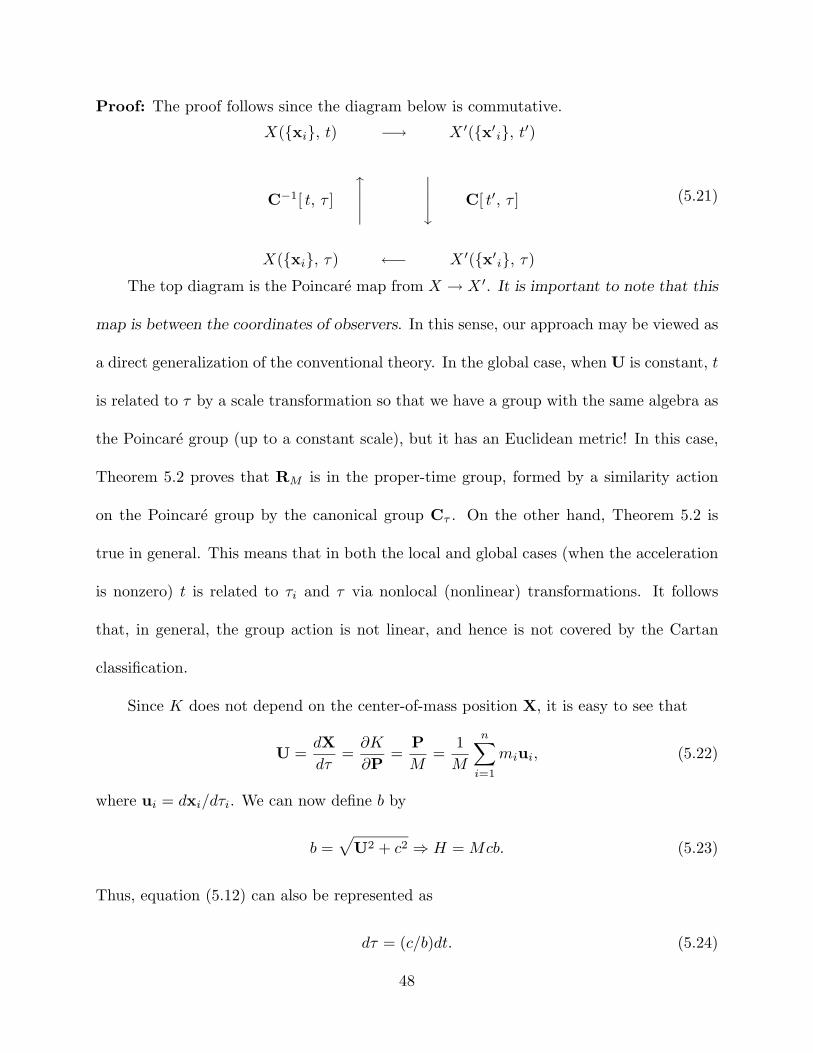
Proof: The proof follows since the diagram below is commutative.

X(xi, t) −→ X ′(x′i, t′)

C−1[ t, τ ]

#% C[ t′, τ ]

X(xi, τ) ←− X ′(x′i, τ)

(5.21)

The top diagram is the Poincare map from X → X ′. It is important to note that this

map is between the coordinates of observers. In this sense, our approach may be viewed as

a direct generalization of the conventional theory. In the global case, when U is constant, t

is related to τ by a scale transformation so that we have a group with the same algebra as

the Poincare group (up to a constant scale), but it has an Euclidean metric! In this case,

Theorem 5.2 proves that RM is in the proper-time group, formed by a similarity action

on the Poincare group by the canonical group Cτ . On the other hand, Theorem 5.2 is

true in general. This means that in both the local and global cases (when the acceleration

is nonzero) t is related to τi and τ via nonlocal (nonlinear) transformations. It follows

that, in general, the group action is not linear, and hence is not covered by the Cartan

classification.

Since K does not depend on the center-of-mass position X, it is easy to see that

U =dXdτ

=∂K

∂P=

PM

=1M

n∑i=1

miui, (5.22)

where ui = dxi/dτi. We can now define b by

b =√

U2 + c2 ⇒ H = Mcb. (5.23)

Thus, equation (5.12) can also be represented as

dτ = (c/b)dt. (5.24)

48

If we set vi = dxi/dτ , an easy calculation shows that

ui =dxi

dτi=

dτ

dτi

dxi

dτ=

bi

bvi ⇒

ui

bi=

vi

b. (5.25)

The velocity vi is the one our observer sees when he uses the global proper-clock of

the system to compute the particle velocity, while ui is the one seen when he uses the local

proper clock of the particle to compute its velocity. Solving for ui and bi in terms of vi

and b, we get

ui =cvi√

b2 − v2i

, bi =cb√

b2 − v2i

orbi

b=

c√b2 − v2

i

. (5.26)

Note that, since b2 = U2 + c2, if U is not zero, then any vi can be larger than c. On

the other hand, if U is zero, b = c and, from the global perspective, our theory looks like

the conventional one. Using (5.26), we can rewrite U as

U =1M

n∑i=1

miui =1M

n∑i=1

micvi√b2 − v2

i

=1M

n∑i=1

bimivi

b=

1H

n∑i=1

Hivi. (5.27)

It follows that the position of the center-of-mass (energy) satisfies

X =1H

n∑i=1

Hixi + Y,dYdτ

= 0. (5.28)

It is natural to choose Y so that X is the canonical center of mass:

X =1H

n∑i=1

Hixi +c2(S × P)

H(Mc2 + H), (5.29)

where S is the (conserved) spin of the system. The important point is that (X,P, τ, K) is

the new set of (global) variables for the system.

Theorem 5.3 If S = (mc2−K)τ , then S is the generator for the change of variables from

(xi, pi, t,H) → (xi, pi,τ ,K), from (X,P, t,H) → (X,P, τ ,K), and:

n∑i=1

pidxi − Hdt =n∑

i=1

pidxi − Kdτ + dS, (5.30)

49

P · dX − Hdt=P · dX − Kdτ + dS. (5.31)

We can now write down the transformations that fix the proper-time of the system of

particles for any observer. If V is the relative velocity between two observers, we have

b′ = γ(V)[b − U · V/c

], b = γ(V)

[b′ + U′ · V/c

], (5.32)

X′ = γ(V)[X† − (V/c)bτ

], X = γ(V)

[X′† + (V/c)b′τ

], (5.33)

U′ = γ(V)[U† − (V/c)b

], U = γ(V)

[U′† + (V/c)b′

]. (5.34)

As our system is closed, U is constant and τ is linearly related to t. Yet, the physical

interpretation is different in the extreme if U is not zero. Furthermore, we see from

equation (5.34) that, even if U is zero in one frame, it will not be zero in any other frame

that is in relative motion. It is clear that τ is uniquely determined by the particles in

the system and is available to all observers. Just as important is the fact that there is a

very basic relationship between the global system clock and the clocks of the individual

particles. In order to derive this relationship, we return to our definition of the global

Hamiltonian K and let W be any observable. Then

dW

dτ= K, W =

H

Mc2H, W =

H

Mc2

n∑i=1

Hi, W

=H

Mc2

n∑i=1

mic2

Hi

[Hi

mic2Hi, W

]=

n∑i=1

Hmi

MHiKi, W

. (5.35)

Using the (easily derived) fact that dτi/dτ = Hmi/MHi = bi/b, we get

dW

dτ=

n∑i=1

dτi

dτKi, W. (5.36)

Equation (5.36) is very important because it relates the global systems dynamics to the

local systems dynamics and provides the basis for a direct approach to the quantum rela-

tivistic many-body problem using one (universal) wave function. The use of a many-times

50

approach is not new and dates back to the early work of Dirac et al56. Our many-times

approach is like that of Rohrlich and Horwitz57 (see also Longhi et al58). Our approach is

distinct, as is clear from (5.36) and the fact that all our times are unique and invariant for

all observers.

5.3 Interaction (Global External)

In this section, we follow convention (in the simplest fashion) and introduce an external

global interaction via minimal coupling in the free Hamiltonian. This means that we fix the

position X, the momentum P, and the mass M. It is still possible for the angular momentum

J to be conserved but, in general, it need not be equal to the angular momentum in the

noninteracting case. Our interaction Hamiltonian becomes

K =Π2

2M+ Mc2 + V (X), (5.37)

where A = A(X, τ), V = V (X, τ) are the vector and scalar potentials of the external field,

and Π = P − (q/c)A. (In the next section, we derive an alternative equation appropriate

when the cause of the external field is included in the theory to form a closed system.)

Using (5.37) and Hamilton’s equations, we get

X = U =ΠM

, P = −∇Π2

2M−∇V. (5.38)

Using standard vector identities, elementary calculations give the (proper-time) Lorentz

force

Mc

b

dUdτ

= qE +q

bU × B, (5.39)

E = −1b

∂A∂τ

−∇V, B = ∇× A. (5.40)

51

The fact that we can derive (a generalized form of) the Lorentz force from a (appar-

ently) nonrelativistic Hamiltonian is well-known (see Hughes59). However, in order to see

how the nonuniqueness of the Maxwell-Lorentz theory shows up here, we need only recall

that W/c = U/b and (1/b)∂/∂τ = (1/c)∂/∂t, so we can also write equations (5.39) and

(5.40) as (W = dX/dt)

MdUdt

= qE +q

cW × B, (5.41)

E = −1c

∂A∂t

−∇V, B = ∇× A. (5.42)

This is the ”original” force derived by Lorentz3 (in 1892) and used as a part of his theory

of the electrodynamics and optics of macroscopic phenomena. What is truly remarkable

is the fact that the two equations (5.39) and (5.41) are mathematically equivalent, but

clearly not physically equivalent, with radically different physical interpretations.

Global Field Theory

We can now discuss the fields of our global system of particles in a given external field.

Using (1/c)(∂ /∂t) = (1/b)(∂ /∂τ) (as in the one-particle case), we can write Maxwell’s

equations for the global system of particles as:

∇ · B = 0, ∇× E +1b

∂B∂τ

= 0, (5.43a)

∇ · E = 4πρ, ∇× B =1b

[∂E∂τ

+ 4πJ]

, (5.43b)

where ρ and J represent the charge and current density of the system (as a whole) relative

to its external environment. Taking the curl of the last equations of (5.43a) and (5.43b),

using the standard vector identity (for any sufficiently differentiable W)

∇× (∇× W) = ∇(∇ · W) −∇2W,

52

and the first equations of (5.43a) and (5.43b), we get the corresponding global wave equa-

tions1b

∂

∂τ

[1b

∂E∂τ

]−∇2 · E = −∇(4πρ) − 1

b∂

∂τ

[4πJb

],

1b

∂

∂τ

[1b

∂B∂τ

]−∇2 · B =

1b

∂

∂τ

[4π∇× J

b

].

(5.44)

Computing the derivatives, these equations may also be written as

1b2

∂2E∂τ2

−[Ub4

· dU∂τ

] [∂E∂τ

]−∇2E = −∇(4πρ) − 1

b

∂

∂τ

[4πJb

],

1b2

∂2B∂τ2

−[Ub4

· dU∂τ

] [∂B∂τ

]−∇2B =

1b

∂

∂τ

[4π∇× J

b

].

(5.45)

From (5.45), we see directly that the dissipative term does not depend on the gauge.

These equations imply that the field of the global system dissipates energy (radiation)

throughout the enclosing domain. Since U= (1/M)∑n

i=1 miui, this radiation depends on

the average of the (local proper) motion of all the particles in the system (e.g., ui =

dxi/dτi). This suggests that the particles live in a heat bath of radiation created by the

global system’s (inertial) reaction to the external field. This heat bath will fill out any

domain enclosing the system of particles.

When U is constant, U = 0 so that there are only velocity fields (and no radiation

fields). This is necessarily the case if energy is conserved on the global level and implies

the following theorem:

Theorem 5.4 If U is constant then all radiation generated by internal interactions must

be absorbed by the particles in the system.

The above theorem was a (required) postulate for the Wheeler-Feynman formulation.

It should be noted that our formulation does not require advanced fields. As will be seen

in the next Section, the individual particle interaction from the local point of view (using

53

the particle proper-time), is of the local field type. In Section 5.5, we will see that the

individual particle interaction, from the global point of view (using the global proper-

time), is of the action-at-a-distance type. This confirms and refines the Wheeler-Feynman

conjecture concerning the relationship between these two views.

It is clear that, in general, the above theorem is only approximately true and it is

more reasonable to consider conservation of energy in a statistical sense. For example,

our galaxy is clearly not a conserved system in the absolute sense, but may be considered

conserved in the mean. Thus, the radiation we receive from the other galaxies is, on the

average, equal to the radiation leakage from our galaxy.

5.4 Interaction (Internal)

In this section we assume that the system of n interacting particles can be represented via:

H =n∑

i=1

Hi = H0 + V, Hi = Hoi + Vi,

H0i =√

c2π2i + m2

i c4, πi = pi −

ei

cAi,

(5.46)

H0 =n∑

i=1

H0i, Ai =∑i =j

Aji, eiAji =eiej (wj − wi)

2sji,

V =n∑

i=1

Vi, Vi =∑i =j

eiej

2sij, sji = sij ,

∂

∂xi(sij) = − ∂

∂xj(sij).

(5.47)

Since we have specified the internal interactions, it is not a priori clear that the

system is closed. Under the stated conditions, the following results can be proven by

direct computation.

Lemma 5.1 Set P =n∑

i=1

pi, Π =n∑

i=1

πi, then Π = P.

Theorem 5.5 H,P = 0, H, V = 0, P, V = 0.

54

It follows that, as in Section 5.2, we can define the total effective mass M by Mc2 =

√H2 − c2P2, so that H =

√c2P2 + M2c4.

Lemma 5.2 H, M = 0, P, M = 0.

Using the above results, it now follows that the set Hi| 1 ≤ i ≤ n, forms a closed system

satisfying all the conditions of Section 5.2.

5.5 Particle Interaction (Local View)

We are now ready to investigate the nature of the dynamics of the ith-particle (say) caused

by the action of the other particles on it. Since there are two possible clocks, τ and τi,

there are two different views, or answers, to our question. Let Wi be any observable of the

ith-particle, thendWi

dτ= K, Wi =

n∑j=1

∂K

∂pj

∂Wi

∂xj− ∂K

∂xj

∂Wi

∂pj,

dWi

dτi= Ki, Wi =

∂Ki

∂pi

∂Wi

∂xi− ∂Ki

∂xi

∂Wi

∂pi,

(5.48)

K =H2

2Mc2+

Mc2

2, Ki =

H2i

2mic2+

mic2

2. (5.49)

The equations of motion can be computed rather easily in the second case. The Hamilto-

nian has an explicit representation as

Ki =π2

i

2mi+ mic

2 +V 2

i

2mic2+

Hi0Vi

mic2,

⇒ dxi

dτi=

∂Ki

∂pi=

πi

mi

(Hi

Hi0

), (5.50)

dpi

dτi= −∂Ki

∂xi= −∇iπ

2i

2mi

(Hi

Hi0

)−∇iVi

(Hi

mic2

). (5.51)

Using (Hi/Hi0)∇iπ2i = −2(ei/c) [(ui · ∇i)Ai + ui × (∇i × Ai)] , Bi = (∇i × Ai),

55

and (Hi/mic2) = (bi/c), we have

dpi

dτi=

ei

c[(ui · ∇i)Ai + ui × Bi] −

bi

c∇iVi. (5.52)

Finally, using (ui · ∇i)Ai = (dAi/dτi) − (∂Ai/∂τi), and Vi = eiΦi, we have

c

bi

dπi

dτi= eiEi +

ei

bi(ui × Bi) , (5.53)

Ei = − 1bi

∂Ai

∂τi−∇iΦi. (5.54)

We call this the local view since it gives information about the action of the external

field on the particle but provides no information about the action of the particle on the

source of the external force. Equation (5.53) is of the same form as (5.39), so if we use

(1/bi)(∂/∂τi) = (1/c)(∂/∂t) and (ui/bi) = (wi/c), we have

dπi

dt= eiEi +

ei

c(wi × Bi) , (5.55)

Ei = −1c

∂Ai

∂t−∇iΦi. (5.56)

This is the same result we found in Section 5.3 when we used minimal coupling directly

for the global case. For later reference we return to equation (5.50), solve for πi, and

differentiate, to get

πi = miui − miui

[(ui · ∇i)Vi

Hi

], mi = mi

(1 − Vi

Hi

). (5.57)

Putting this term in (5.53), and taking the dot product, we have

(ui · ui) =12

d

dτi‖ui‖2 = ‖ui‖2

[(ui · ∇i)Vi

Hi

]+

ei

mi(ui · Ei, ) . (5.58)

mi =c

bimi = mi

c

bi

[1 − Vi

Hi

].

56

5.6 Particle Interaction (Global View)

Let us now see what changes occur when we focus on the motion of the same particle as

seen from the global point of view. In this case, we have

dxi

dτ= vi =

∂K

∂pi=

(H

M

)πi

Hi0, (5.59)

dpi

dτ= −∂K

∂xi= −

(H

Mc2

) n∑k=1

[c2∇iπ

2k

Hk0−∇iVk

]. (5.60)

Using standard calculations as in the local view, and (H/Mc2) = (b/c), we have

dpi

dτ=

n∑k=1

ek

c[(vk · ∇i)Ak + vk × (∇i × Ak)] − b

c∇iVk

. (5.61)

Now use

(vi · ∇i)Ai = (dAi/dτ) − (∂Ai/∂τ),

to getdpi

dτ− ei

c

dAi

dτ=

ei

c[vi × Bi] −

ei

c

∂Ai

∂τ− b

c∇iVi

+n∑

k =i

ek

c[(vk · ∇i)Ak + vk × (∇i × Ak)] − b

c∇iVk

.

(5.62)

From, (5.46) and (5.47) we see that (vk · ∇i)Ak = −(vk · ∇k)Aik, etc, so we may

write (5.62) in the form (using Ei = −(1/b)(∂Ai/∂τ) −∇iΦi,Bi = vi × Ai )

c

b

dπi

dτ= eiEi +

ei

b[vi × Bi]

−n∑

k =i

ek

b[(vk · ∇k)Aik + vk × (∇k × Aik)] − ek∇kΦik

.

(5.63)

If we now set (vk · ∇k)Aik = (dAik/dτ) − (∂Aik/∂τ), Bik = ∇k × Aik, Eik =

−(1/b)(∂Aik/∂τ) −∇kΦik, and Fik = ekEik + (ek/b)vk × Bik, we have

c

b

dπi

dτ= Fi −

n∑k =i

Fik +

ek

b

dAik

dτ

. (5.64)

57

If we use πi = miui, mi = mi [1 − Vi/Hi] , ui =[cvi

/(b2 − v2

i )1/2

], we get (b is constant)

d

dτ

mivi√

1 −(v2

i

/b2

) = Fi −

n∑k =i

Fik +

ek

b

dAik

dτ

, mi =

(c

b

)2

mi. (5.65)

In order to interpret equation (5.65), we return to equation (5.54) and use the fact

that (1/bi)(∂/∂τi) = (1/b)(∂/∂τ) and (ui/bi) = (vi/b) to get

− 1bi

∂Ai

∂τi−∇iΦi = −1

b

∂Ai

∂τ−∇iΦi,

ei

bi(ui × Bi) =

ei

b(vi × Bi) .

This means that our force Fi in (5.65) is identical to the right-hand side of (5.53) (the local

Lorentz force). Equation (5.65) is our replacement for the Lorentz-Dirac equation. The

second term on the right-hand side is the necessary dissipative term required to satisfy

Newton’s third law, and represents the action of the i-th particle on all the other particles

in the system. It is important to note that this equation contains no third-order derivatives,

so that it will satisfy the standard conditions for existence and uniqueness of solutions for

initial value problems. It will not contain runaway solutions, nor advanced actions, etc.

Furthermore, the equation does not depend on the structure of the particles in the system.

We now see that the global view of particle interactions is a pure action-at a- distance

theory while from the local point of view particle interactions are mediated by the fields

(a field theory).

For future reference, we assume that the global system is interacting with an external

force, so that U is not zero. If we differentiate the left-hand side of (5.65), we get ( using

(β2

i = v2i

/b2

)),

c

b

dπi

dτ=

mivi[1 − β2

i

]1/2+

mivi

[vi · vi − U · U

]b2

[1 − β2

i

]3/2

− mivi[1 − β2

i

]1/2

d

dτ

[ln

(1 − Vi

Hi

)], mi = mi

c2

b2

(1 − Vi

Hi

).

(5.66)

58

Taking the dot product with vi, we obtain the effective power transfer for the i-th particle

mi

2[1 − β2

i

]3/2

d ‖vi‖2

dτ−

mi ‖vi‖2[U · U

]b2

[1 − β2

i

]3/2− mi ‖vi‖2[

1 − β2i

]1/2

d

dτ

[ln

(1 − Vi

Hi

)]

= vi · Fi −n∑

k =i

vi · Fik +

ek

b

(vi ·

dAik

dτ

).

(5.67)

If U = 0, (5.64) and (5.67) become (β2i = v2

i

/c2, mi = mi, and τ = t)

d

dt

(mivi√1 − β2

i

)= Fi −

n∑k =i

Fik +

ek

c

dAik

dt

, (5.68)

mi

2[1 − β2

i

]3/2

d ‖vi‖2

dt− mi ‖vi‖2[

1 − β2i

]1/2

d

dt

[ln

(1 − Vi

Hi

)]

= vi · Fi −n∑

k =i

vi · Fik +

ek

c

(vi ·

dAik

dt

).

(5.69)

It follows that, even when the global system is at rest in the frame of the observer, our

theory is distinct. In closing this section we note that summing equation (5.65) or (5.68)

on i gives zero as expected, reflecting conservation of the global momentum.

6.0 Discussion

6.1 Proper-time of the Source

In this paper, we have shown that Maxwell’s equations have a mathematically equivalent

formulation and additional symmetry group that fixes the proper-time of the source for

all observers. The new group is closely related to the Lorentz group and, in fact, at the

local level, is a nonlinear and nonlocal representation. We have constructed a dual theory

using the proper-time of the source and have shown that it is covariant with respect to this

group. However, the speed of light now depends on the motion of the source and the new

59

group replaces time transformations between observers by transformations of the velocity

of light with respect to the source for different observers. This implies that the speed of

light can be greater than its value in any fixed inertial frame. In the new formulation, the

second postulate of the special relativity is only true when the source is in the rest frame

of the observer. We have further shown that, for any closed system of particles, there is

a global inertial frame and unique (invariant) global proper-clock (for each observer) from

which to observe the system. In this case, the corresponding group differs from the Lorentz

group by a scale transformation. This global proper-clock is intrinsically related to the

proper-clocks of the individual particles in the system and provides a unique definition of

simultaneity for all events associated with the system. Hence, at the global level, we can

always choose a unique observer-independent measure of time for the study of physical

systems. One important consequence of this result can be stated as a theorem.

Theorem 6.1 Suppose that the observable universe is representable in the sense that the

observed ratio of mass to total energy is constant and independent of our observed portion

of the universe. Then the universe has a unique clock that is available to all observers.

The above assumptions are equivalent to the homogeneity and isotropy of the energy and

mass density of the universe.

The use of a global variable without attaching physical meaning to it dates back to

the early work of Tetrode and Fock (for a review, see Fanchi51). However, starting in

the 1970’s, Horwitz and Piron60 and later Fanchi51 began to suggest the use of a special

clock for global systems which they called the historical time. They predicted that such a

variable should exist as a real physical parameter and Fanchi52 suggested experiments to

60

detect this clock. In our approach we treat the transformation from observer proper-time

to global system proper-time as a canonical (contact) transformation on extended phase

space. This approach allows us to identify the canonical Hamiltonian and the associated

Lie algebra (Poisson) bracket. Hence, we suggest that this global proper-time is the one

sought by the above researchers. From an operational point of view, all observers can

identify the time according to this (global) clock by recording the time on their clock, use

the experimentally determine value for the velocity W , of the center of mass of the system,

and then use equation (1.3a).

Rohrlich61 has recently conducted a very interesting study of the classical self-force

for the dynamics of finite-sized particles with both electromagnetic and gravitational self-

interactions (using the Lorentz-Dirac equation). He posits his model as a replacement for

the point-particle model which is beyond the validity of the classical theory. His approx-

imations neglect the nonlinear terms in the derivatives of the acceleration and leads to

more reasonable equations of motion, but violates time-reversal invariance. This suggests

that a successful classical theory which does not require the point-particle concept may

help to explain time-reversal noninvariance at the macro-level.

As noted earlier, the proper-time theory does not depend on the size, structure, or

geometry of the charge distribution. Furthermore, the global fields of any system of radi-

ating particles in a closed domain will quickly leak radiation into every part of the domain.

Since the field equations carry intrinsic information about the velocity and acceleration

of each particle at the moment of dissipation, any observer will only receive information

about the past behavior of the particles in the system. Since the observed radiation is

61

an average over all the particles, this provides an explanation for the arrow of time as a

statistical effect as suggested by Einstein. Also, since we only use the retarded solutions of

Maxwell’s equations, we may follow the suggestion of Feynman32 and Stuckelberg62 and

treat antimatter as matter with its proper-time reversed.

The above approach also provides us with a simple answer for questions about con-

servation laws during the big bang. If we assume that the big bang created two separate

universes, one with matter (moving forward in proper-time), and one with antimatter

(moving backward in proper-time). Then all global (physical) quantities in our universe

will be conserved while providing us with a nice explanation for the lack of large concen-

trations of antimatter in our universe.

6.2 Equivalent Theories and Convention

It is no doubt more unsettling to many that the two theories could be mathematically

equivalent but not physically equivalent. It is more natural to expect that two mathemat-

ically equivalent theories would also be physically equivalent, and there are a number of

historical examples to support such expectations; the Lagrange-Hamiltonian formulation

of classical mechanics, the Heisenberg-Schrodinger formulation of quantum mechanics, and

the Feynman-Schwinger-Tomonaga formulation of quantum electrodynamics. In the first

case, both formulations have proved equally valuable depending on the purpose. However,

the latter two cases raise interesting questions.

After Feynman constructed a path integral formulation of quantum mechanics, it

was shown to physically include the Heisenberg-Schrodinger formulation. However, it

has never been shown to be mathematically equivalent since there are well-known serious

62

foundational problems with the mathematical notion of a path integral for quantum theory.

On the other hand, it has not been shown that the Heisenberg-Schrodinger formulation is

physically equivalent to the Feynman path integral approach. (There are theories where the

path integral approach is easy, while the other two approaches are difficult to construct.)

In order to prove that the Feynman formulation of QED was physically equivalent

to the Schwinger-Tomonaga formulation, Dyson63 assumed that time had the additional

property of an index which kept track of the time an operator operates (time-ordering).

This represents a new physical input to theory formulation and has only recently received

any mathematical attention64,65,66. Thus, mathematical equivalence has not been shown,

and although some progress has been made, we are far from a solution.

In our opinion, the Feynman path integral approach is physically more general than

that of Heisenberg and Schrodinger, and his formulation of QED is physically more general

than that of Schwinger and Tomonaga. In both cases, he introduces new concepts that

make it physically easier to think about and solve problems. What Feynman did was to

show that it is still possible to formulate theories which more closely represent the way the

world appears to us in our consciousness.

It was Poincare67 who first noticed that some hypotheses (assumptions), which are

made for theory construction, arise because of empirical data, while others occur because

they are convenient. The convenient hypotheses are generally imposed by the mathematical

structures we use to represent physical theories. These hypotheses are called conventions

by Poincare in order to point out the fact that different conventions could lead to different

theories which would be mathematically equivalent. He was not sure that the theories

63

would be physically different, but he seems to have left open that possibility. The work of

this paper shows that different conventions can lead to different physical theories. Since

all inerital reference frames are equivalent, the one chosen by any observer is a convention.

If we seek simplicity, we can all attach our frames to the MBR and use the proper-time

of the universe for our global clock. In this case, we could satisfy the two postulates of

the special theory, while the field and particle equations of any system would be invariant

under the action of the Lorentz group (for all observers).

6.3 Velocity of Light

The price paid for the results of this paper will certainly seem high to many. We have

rejected the third postulate of Minkowski that time be put on an equal footing with

position and made a coordinate for four-geometry. We have also rejected the assumption

(convention) that the observer proper-time be used to define the dynamics of an observed

system. Thus, in our approach, the time is a (intrinsic) dynamical variable which must be

determined by experiment along with other properties (of the observed system). This leads

to a new interpretive framework in which the second postulate is only true when the source

is at rest in the frame of the observer. Thus, we have reduced the observer reference frame

to the prerelativistic three-geometry of Euclidean space. The observer’s clock is now a part

of the measuring equipment which is used to determined the proper-time of the source.

The proper-time formulation has an obvious disadvantage since, it is generally believed

that, all the available experimental evidence supports the second postulate of special rel-

ativity (that the velocity of light is constant). Einstein68 pointed out in a footnote to his

second paper: “The principle of the constancy of the velocity of light is of course con-

64

tained in Maxwell’s equations.” What he meant by this was that the second postulate

follows from the fact that the constant c in Maxwell’s equations is an invariant for all

(inertial) observers. Since that time, many experiments have been done to verify that

assumption. However, in 1965, Fox69 wrote a very important paper which reviewed the

evidence for constant c and against the emission theory of Ritz44. His conclusion was that

all previous experiments were flawed for a number of reasons. In many cases, analysis of

the experimental data failed to take into account the (now well-known) extinction theorem

of Ewald and Oseen (see Jackson2 ). The only data found that firmly supported the second

postulate came from experiments on the lifetime of fast mesons and the velocity of γ rays

and light from moving sources. In his conclusion Fox states that “ · · · Unless something has

been overlooked, these seem to be the only pieces of experimental evidence we have. This

is surprising in light of the long history and importance of the problem.” These “pieces of

experimental evidence” have another interpretation in the proper-time theory. As noted

in Section 1, the lifetime of fast mesons is the fixed value measured when they are at rest

while their velocity is now computed using the proper-time of the meson which is derived

from the experiment. The same interpretation applies to γ rays and light from moving

sources. Thus, the same experiments that support c as constant when we assume that the

observer proper-time should be used to formulate the theory also supports the result that

the speed of light depends on the motion of the source when we assume that the source

proper-time should be used to formulate the theory.

6.4 Photon Mass

Work on the question of photon mass has focused on the addition of a mass term to the

65

Lagrangian density for Maxwell’s equations and generally leads to the Proca equation ( see

Bargmann and Wigner70). Early work in this direction can be traced back from the paper

of Schrodinger and Bass71. As in our approach, the speed of light is no longer constant in

all reference frames. In this case, the fields are distorted by the mass term and experiments

of Goldhaber and Nieto72 use geomagnetic data to set an upper bound of 3 × 10−24 GeV

for the mass term (see Jackiw73 ). This approach causes gauge problems, and has not

found favor at the classical level. The proper-time theory is fully gauge invariant and the

(photon) mass is dynamical, appearing only during acceleration of the source.

It should be recalled that Maxwell’s equations are (spin 1) relativistic wave equations

(see Akhiezer and Berestetskii74). On the other hand, the experiments of Pound and

Snider75 show directly that photons have an apparent weight (as one would expect of any

material object). These experiments do not depend on either the special or general theory

of relativity and are not directly dependent on frequency or wavelength measurements. The

existence of a small mass for the photon has important implications for QED. It is well-

known that a small photon mass can eliminate the infrared catastrophe (see Feynman76).

66

Acknowledments

Work for this paper was begun while the first author was supported as a member

of the School of Mathematics in the Institute for Advanced Study, Princeton, N. J., and

completed during a visting appointment in the physics department at the University of

Michigan. The authors would like to acknowledge important discussions, comments and

encouragement from Professors G. Wienreich and H. Winful of the University of Michigan,

and Professor Horwitz from the University of Tel Aviv, Isreal. We would like to give special

thanks to Professor M. Wegener of the University of Aarhus, Denmark for an introduction

to the work of Poincare.

Appendix

In this appendix, we outline the derivation of (3.54) from the angular distribution (3.52) by

taking the limit as r → ∞ after integrating over a sphere of radius r. The integrations over

the azimuthal angle φ are easily done. Then, for the integrations over the polar angle θ, it

is convenient to make the change of variable µ = cos θ and for a = 2, 3, . . . , b = 0, 1, 2 . . . ,

define the following sequence of integrals:

Ia,b ≡1∫

−1

(1 − βµ)−aµbdµ. (A1)

We then obtain from (3.52) that

67

limr→∞

∫∫−dU

dt(Ω)dΩ =

bq2 |a|2

b4

(1 − 1

2sin2 α

)I4,0

+(

12

sin2 α − cos2 α

)I4,2 − 2β

[β cos2 α (I5,0 − I5,2)

+(− cos2 α +

12

sin2 α

)(I5,1 − I5,3)

]

+ β2

[(β2 cos2 α +

12

sin2 α

)(I6,0 − I6,2)

+ 2β cos2 α (I6,3 − I6,1) +(

cos2 α − 12

sin2 α

)(I6,2 − I6,4)

].

(A2)

Relations among the integrals (A1) for different integer values of a and b are easily obtained

by integration by parts:

Ia,b =1

β (a − 1)

[(1 − β)−(a−1) − (−1)b (1 + β)

]− b

β (a − 1)Ia−1,b−1, (A3)

for a ≥ 2, b ≥ 1; and for b = 0, only the first term contributes:

Ia,0 =1

β (a − 1)

[(1 − β)−(a−1) − (−1)b (1 + β)

], a ≥ 2. (A4)

We note that the differences of the integrals (A1) that occur in (A2) are of the type

Ia,b − Ia,b+2 for given values of a and b. For differences of this type, the term in brackets

in (A3) does not contribute and we have:

Ia,b − Ia,b+2 =1

β (a − 1)[−b (Ia−1,b−1 − Ia−1,b+1) + 2Ia−1,b+1] , (A5)

for integer values of a and b such that a ≥ 3, b ≥ 1. For b = 0 the difference term on the

right hand side of (A5) is missing and we have:

Ia,0 − Ia,2 =2

β (a − 1)Ia−1,1, a ≥ 3. (A6)

68

To use the above results to evaluate (A2), we start with differences of the form (A5)

and (A6) with a = 6 and b = 1, 2. The terms which arise from the difference term on

the right-hand side of (A5) combine with the terms with a = 5 which are already present

in (A2). After combining the coefficients of similar terms, we can then apply the process

again to the integrals (A1) with a = 5. Now we have a difference from the situation with

the integrals involving a = 6 that , in addition to having differences of the form (A5) with

a = 5 and b = 1 and of (A6) with a = 5, we also have the integrals I5,1 and I5,0 which are

not differences. However, these are easily evaluated by use of (A3) (giving a term involving

I4,0) and (A4), respectively. We can continue this procedure to successively lower values

of a, terminating at the value a = 2. The substitution of the various values of Ia,b and

elimination of cos2 θ by use of the identity cos2 θ = 1 − sin2 θ leads to the result (3.54).

69

References

[1] R. P. Feynman, R. B. Leighton, and M. Sands, The Feynman Lectures on Physics,

Vol II. Addison-Wesley, New York (1974).

[2] J. D. Jackson, Classical Electrodynamics, John Wiley & Sons, New York (1975).

[3] H. A. Lorentz, Archives Neerlandaises des Sciences Exactes et Naturelles, 25, 353

(1892).

[4] H. A. Lorentz, The Theory of Electrons B. G. Teubner, Leipzig, 1906; (reprinted by

Dover, New York, 1952).

[5] A. Einstein, Ann. d. Phys. 17, 891 (1905).

[6] D. E. Spencer and U. Y. Shama, Physics Essays 9, 476 (1996).

[7] A. Einstein, Jahrbuch Radioaktivitat V, 422 (1907) (Berichtigungen).

[8] H. Poincare, C.R. Acad. Sci. Paris 140, 1504 (1905).

[9] H. Minkowski, Physikalische Zeitschrift 10,104 (1909).

[10] E. Whittaker, A History of Aether and Electricity, Vol. I, Thomas Nelson and Sons,

London, (1951).

[11] M. Dresden, in Renormalization: From Lorentz to Landau (and Beyond), L. M. Brown

(ed.), Springer-Verlag, New York, (1993).

[12] M.H.L. Pryce, Proc. Roy. Soc. London A 195, 400 (1948).

[13] P. A. M. Dirac, Rev. Mod. Phys. 21, 392 (1949).

[14] H. Leutwyler and J. Stern, Ann. Phys. (N. Y.) 112, 94 (1978).

[15] B. Bakamjian and L. H. Thomas, Phys. Rev. 92, 1300 (1953).

70

[16] D. G. Currie, T. F. Jordan, and E. C. G. Sudarshan, Rev. Mod. Phys. 35, 350 (1963).

[17] E. C. G. Sudarshan and N. Mukunda, Classical Dynamics: A Modern Perspective.

John Wiley & Sons, New York (1974).

[18] R. Fong and J. Sucher, J. Math. Phys. 5, 456 (1964).

[19] A. Peres, Symposia Mathematica 12, 61 (1973).

[20] E. P. Wigner, in Aspects of Quantum Theory, in Honor of P. A. M. Dirac’s 70th

Birthday, edited by A. Salam and E. P. Wigner (Cambridge Univ. Press, London,

1972).

[21] F. Rohrlich,Classical Charged Particles: Foundations of Their Theory , Addison-

Wesley, Reading, Massachusetts (1965).

[22] S. Parrott, Relativistic Electrodynamics and Differential Geometry, Springer, New

York (1987).

[23] F. Rohrlich, Phys. Rev. D 58, 116002 (1999).

[24] W. K. H. Panofsky and M. Phillips, Classical Electricity and Magnetism, (Second

Edition), Addision-Wesley, Reading, MA. (1962).

[25] J. A. Wheeler and R. P. Feynman, Rev. of Mod. Phys. 21, 425 (1949).

[26] J. Schwinger, Found. Phys. 13, 2573 (1998).

[27] M. Born and L. Infield, Proc. R. Soc. London A144, 425 (1934).

[28] P. A. M. Dirac, Proc. R. Soc. London A167, 148 (1938).

[29] F. Bopp, Ann. d. Phys. 42, 573 (1942).

[30] N. Rosen, Phys. Rev. 72, 298 (1947).

71

[31] B. Podolsky and P. Schwed, Rev. Mod. Phys. 20, 40 (1948).

[32] R. P. Feynman, Phys. Rev. 74, 939 (1948).

[33] R. Haag, Z. f. Naturf. 10a, 752 (1955).

[34] S. Parrott and D. J. Endres, Found. Phys. 25, 441 (1995).

[35] F. E. Low, Ann. Phys. 266, 274 (1998).

[36] A. A. Penzias and R. W. Wilson, Ap. J. 142, 419 (1965).

[37] P.J.E. Peebles, Principles of Physical Cosmology, Princeton University Press, London

(1993).

[38] S. Schweber, QED And The Men Who Made It , Princeton University Press, London

(1994).

[39] B. French and V. Weisskopf, Phys. Rev. 75, 1240 (1949).

[40] N. Kroll and W. Lamb, Phys. Rev. 75, 388 (1949).

[41] P. A. M. Dirac, Sci. Amer. 208, 45 (1963).

[42] T. P. Gill, The Doppler Effect , Logos Press, London (1965).

[43] G. A. Schott, Phil. Mag. 29, 49 (1915).

[44] W. Ritz, Archives des Sciences Physiques et Naturelles 16, 209 (1908).

[45] C. Moller, The Theory of Relativity, Oxford Clarendon Press, London (1960).

[46] C. H. Papas, Theory of Electromagnetic Wave Propagation, Dover Press, New York

(1988).

[47] R. Courant and D. Hilbert, Methods of Mathematical Physics, vol. II , Wiley-

Interscience, New York (1965).

72

[48] T. L. Gill and J. Lindesay, Inter. J. Theor. Phys. 32, 2087 (1993).

[49] T. L. Gill, Fermilab-Pub-82/60-THY.

[50] J. P. Aparicio, F. H. Gaioli, and E. T. Garcia-Alvarez, Phys. Rev. A 51, 96 (1995).

[51] J. R. Fanchi, Parametrized Relativistic Quantum Theory, Kluwer, Dordrecht, (1993).

[52] J.R. Fanchi, Found. Phys. 23, 487 (1993).

[53] E. P. Wigner, Ann. Math. 40, 149 (1939).

[54] G. L. Strobel, Inter. J. Theor. Phys. 37, 2087 (1998).

[55] T. L. Gill, W.W. Zachary, and J. Lindesay, Inter. J. Theor. Physics 37, 2573 (1998).

[56] P. A. M. Dirac, V. A. Fock, and B. Podolsky, Phys. Z. Sowj. Un. 2, 6 (1932) [Reprinted

in J. Schwinger, ed. Selected Papers in Quantum Electrodynamics, Dover, New York

(1958)].

[57] F. Rohrlich and L. P. Horwitz, Phys. Rev. D 24, 1528 (1981).

[58] G. Longhi, L. Lusanna, and J. M. Pons, J. Math. Phys. 30, 1893 (1989).

[59] R. J. Hughes, Amer. J. Phys. 60, 301 (1992).

[60] L. P. Horwitz and C. Piron, Helv. Phys. Acta 46, 316 (1981).

[61] F. Rohrlich, Phys. Rev. D 60, 084017 (1999).

[62] E. C. G. Stuckelberg, Helv. Phys. Acta 15, 23 (1942).

[63] F. J. Dyson, Phys. Rev. D 75, 486, 1736 (1949).

[64] G. W. Johnson and M. L. Lapidus, Mem. Amer. Math. Soc. 62, 1 (1986).

[65] T. L. Gill and W.W. Zachary, J. Math. Phys. 28, 1459 (1987).

73

[66] G. W. Johnson and M. L. Lapidus, The Feynman Integral and Feynman’s Operational

Calculus, Oxford U. Press, New York, (2000).

[67] H. Poincare, Science and Hypothesis, Dover Press, New York, (1952).

[68] A. Einstein, Ann. d. Phys. 18, 639 (1905).

[69] J. G. Fox, Amer. J. Phys. 33, 1 (1965).

[70] V. Bargmann and E. P. Wigner, Proc. Nat. Acad. Sci. 34, 211 (1948).

[71] E. Schrodinger and L. Bass, Proc. R. Soc. London A232, 1 (1938).

[72] A. Goldhaber and M. Nieto, Rev. Mod. Phys. 43, 277 (1971).

[73] R. Jackiw, Comments Mod. Phys. 1A, 1 (1999).

[74] A. I. Akhiezer and V. D. Berestetskii, Quantum Electrodynamics, Wiley-Interscience,

New York (1965)

[75] R. V. Pound and J. L. Snider, Phys. Rev. 140, B788 (1965).

[76] R. P. Feynman, Quantum Electrodynamics, W. A. Benjamin, New York (1964)

74