A SEMI-CLASSICAL STUDY OF ELECTRON BLURRING IN THELONGITUDINAL STERN-GERLACH MAGNET

by

Daniel Wm. James

Submitted to the Department of Physics and Astronomy in partial

fulfillment of graduation requirements for the degree of

Bachelor of Science

Brigham Young University

November 2004

Advisor: Jean-Francois Van Huele Thesis Coordinator: Justin Peatross

Signature: Signature:

Department Chair: Scott D. Sommerfeldt

Signature:

Abstract

We study the feasibility of polarizing electron beams using the lon-gitudinal Stern-Gerlach effect. After a brief historical motivation wereview a semi-classical analysis for electron dynamics in the presenceof an axial current ring. We derive the complete set of differentialequations for the trajectories and variances in this cylindrical geome-try and point out differences with expressions found in the literature.We solve a subset of the equations numerically for a particular choiceof initial conditions and we provide numerical simulations of the ef-fect. We conclude by comparing the trajectory variance with the spinseparation.

ii

Acknowledgements

I would like to thank Dr. Van Huele for never giving up on me. Thankyou so very much. I would also like to thank Allison Jarstad, for inspiringme to finish what I had begun and to continually improve myself. You trulyare a great friend.

iii

Contents

1 Introduction 1

2 Background 12.1 Electron Polarization in Early Quantum Theory . . . . . . . . 12.2 Brillouin’s Proposal . . . . . . . . . . . . . . . . . . . . . . . . 22.3 Pauli’s Refutation . . . . . . . . . . . . . . . . . . . . . . . . . 22.4 Problems with Pauli’s Refutation . . . . . . . . . . . . . . . . 3

3 Semi-Classical Method 4

4 Current Ring Dynamics 6

5 Dynamical Equations 7

6 Numerical Solutions 106.1 Spin Separation . . . . . . . . . . . . . . . . . . . . . . . . . . 106.2 Matlab . . . . . . . . . . . . . . . . . . . . . . . . . . . . . . . 10

7 Analysis 117.1 A Typical Result . . . . . . . . . . . . . . . . . . . . . . . . . 117.2 Possible Improvements . . . . . . . . . . . . . . . . . . . . . . 11

8 Conclusion 11

A Appendices 13A.1 3-Dimensional Taylor Expansion for a General Function . . . . 13A.2 Commutation Relation of Two 3-Dimensional General Functions 13A.3 Expectation Value of the Commutation Relation between Two

3-Dimensional General Functions . . . . . . . . . . . . . . . . 14A.4 Running Matlab sources . . . . . . . . . . . . . . . . . . . . . 15A.5 Source 1: rhs17.m . . . . . . . . . . . . . . . . . . . . . . . . . 15A.6 Source 2: spin.m . . . . . . . . . . . . . . . . . . . . . . . . . 16

iv

1 Introduction

The truth is rarely appreciated, and perhaps that is why I feel a little trep-idation in saying that I undertook this project originally with the intent tosolely fulfill a requirement for graduation. However, the not so gentle nudgingat times of Dr. Van Huele and the ability to utilize the limited mathematicalknowledge that I have accumulated sufficiently excited me to take on a purelytheoretical project. Throughout my academic career though, I had yet to un-dertake such an ambitious project as a senior thesis where the research andlearning environments were entirely unstructured and self-imposed. In orderto step-up and not become a victim of these circumstances I surrounded my-self with caring people who inspired me to continue. People who eventuallybecame my why’s.

Within this paper you will find the historicity of electron beam polariza-tion: where the idea was first generated, discussed, dashed, and once againslightly pried back open to the realm of possibility as discussed in the Back-ground section. The development of a method for analyzing a mostly classi-cal system with some quantum correction will be found in the Semi-ClassicalMethod section. Its application to a specific apparatus, the LongitudinalStern-Gerlach, will be covered in section four, Current Ring Dynamics. Theequations of motion describing the electron beam in the Longitudinal Stern-Gerlach is discussed in section five, Dynamical Equations. The numericalsolutions and the chosen method of solution for the equations of motion arefound in the Numerical Solutions section, and in the Conclusion the questionconcerning the possibility of polarizing an electron beam will be presentedbased upon the results.

2 Background

2.1 Electron Polarization in Early Quantum Theory

Throughout the formative years of quantum theory, several of its discoverersdebated at length the possiblity of polarizing an electron beam. Stern andGerlach had polarized a beam of neutral silver atoms using what has cometo be known as a transverse Stern-Gerlach magnet and it would seem natu-ral to begin our study of electron beam polarization with an apparatus thathas already proven capable of beam polarization. However, the transverse

1

Stern-Gerlach magnet is unable to decouple the splitting of the beam of freeelectrons from the blurring induced by the Lorentz force acting on a beam offinite width [3, 4, 5]. In order to circumvent the Lorentz force blurring Bril-louin suggested a new experimental geometry, the longitudinal Stern-Gerlachwhere the magnetic inhomogeneity that generates the splitting is in the di-rection of propagation thereby minimizing the blurring force [6]. In responseto this suggestion, the outspoken Pauli said, ”it is impossible to observe thespin of the electron, separated fully from its orbital momentum, by meansof experiments based on the concept of classical particle trajectories”[1]. Inshort, Pauli found that the longitudinal Stern-Gerlach would not polarize anelectron beam. So the question remained dormant for years until Dehmeltdid what Pauli thought unthinkable. Dehmelt isolated electrons of a givenspin in a modified Penning trap (continuous Stern-Gerlach magnet) and mea-sured their magnetic moment ~µ. Since the measurement of ~µ is so closelyrelated to the measurement of spin splitting, Dehmelt reopened the questionof electron beam polarizability.

2.2 Brillouin’s Proposal

With renewed potential we address Brillouin’s proposal. The longitudinalStern-Gerlach experimental setup is characterized by electrons with a spe-cific energy being passed through an inhomogenous magnetic field at someangle to the principal direction of propagation (z). The kinetic energy of theparticle in the z direction depends solely upon the insertion angle, and thepotential energy depends on the spin projection along z. Electrons with spinparallel to the field require a different minimum insertion angle than thosewith spin antiparallel to it if they are to reach the detector. The differencein distance traveled associated with a given insertion angle effectively servesto split an electron beam by spin.

2.3 Pauli’s Refutation

To understand both the strengths and limitations of the longitudinal Stern-Gerlach we now follow reference [9] in the following argument given by Pauliagainst its potential efficacy given at the Sixth Solvay Conference in 1930. Webegin with a finite width beam of electrons moving in the positive z direction,

2

anti-parallel to the primary magnetic field direction. If ∂Bz

∂z> 0, then elec-

trons with spin parallel to z and velocity vz stop and reverse direction withina time t given by mvz = µB

∂Bz

∂zt, where m is the mass of the electron. The

number of electrons detected beyond vzt is half that which would be countedwhere spin properties are excluded. Now suppose that the magnetic field Bis everywhere parallel to the xz plane, so by Maxwell’s equations we knowthat ∂Bx

∂x= −∂Bz

∂z. If the field at x = 0 is exactly along z, then at a distance

∆x from the z axis the magnetic field component Bx = ∂Bx

∂x∆x = −∂Bz

∂z∆x.

This field causes the velocity in the z direction to reverse sign in the Larmorprecession time. Therefore, forces must act over a time much less than theLarmor precession time, i.e., t ¿ h

µBBx, or equivalently µB(∂Bz

∂z)t∆x ¿ h,

which reduces to mvz∆x ¿ h. Because of the wave nature of electrons thelast condition cannot be fulfilled during the complete interaction time be-cause the de Broglie wavelength λ is just h

mvzand beam widths ∆x ¿ λ are

not possible. However, if you tried to make one, then ∆vx > hm∆x

by theuncertainty principle requires that ∆vx À vz and the outcome cannot bepredicted by classical mechanics.

2.4 Problems with Pauli’s Refutation

This constitutes the whole of Pauli’s argument; however, there exists a pointof questionable reasoning forwarded by Pauli concerning the actual classicaltrajectories. It is certain that an electron slightly displaced from the z-axiswill experience a force that starts to rotate velocity towards the y axis. Thechange in the direction of motion is modified by the small induced vy whichcauses a Lorentz force due to Bz. The resulting trajectory is a helical spiralabout z, with only one direction of motion along z. Since the precessiondoes not affect the result, the forces are not required to act over a time muchless than the Larmor precession time. The uncertainty principle no longerinhibits the dynamics of the system and a time can be chosen that satisfiesthe initial conditions.Therefore the essential difficulty in applying the transverse Stern-Gerlachgeometry to the polarization of a finite electron beam is that Lorentz forcesblur the beam, and in order to circumvent the blurring longitudinal geometryis used. To analyze this experimental situation, we cannot resort to theanalytically simple mixed dynamical picture where the electron trajectory istreated classically and the spin quantum mechanically, nor can we treat the

3

problem entirely quantum mechanically due to the analytical difficulty; so amethod which exhibits partially the advantages of both dynamical picturesis employed which incorporates both classical and quantum mechanics morefully.

3 Semi-Classical Method

This method was originally developed by Sundaram and Milonni [2] for masertheory. More recently though H. Batelaan [7] has employed this method todescribe electron polarization by the longitudinal Stern-Gerlach, the subjectof this paper; we develop this analysis more fully and in the process we correctthe form of some of the equations given in [7]. The purpose of this section isto restate the development of the method and correct the errors previouslymade. We begin by writing the position and momentum operators as the sumof their large classical expectation value and a small quantum correction,

x = 〈x〉+ δx, px = 〈px〉+ δpx, (1)

with the commutation relation [x, px] = [δx, δpx] = ıh. In order to describethe time variance of these operators it is necessary to treat them quantummechanically. Within quantum mechanics there are two equivalent picturesof describing time dependence. The first is the Schroedinger picture wherethe states, ψ(x, t), are time dependent and the physical variables have notime dependence. In this picture the time dependence is described by

ıh∂

∂tψ(x, t) = Hψ(x, t). (2)

The second is the Heisenberg picture. Within this framework the states,ψ(x) are time independent and the physical variables have time dependence,the exact opposite of the Schroedinger picture. The time dependence forHeisenberg is described by

ıhd

dtA = [A, H] + ıh

∂

∂tA (3)

which leads to

ıhd

dt〈A〉 = 〈[A,H]〉+ ıh〈 ∂

∂tA〉. (4)

4

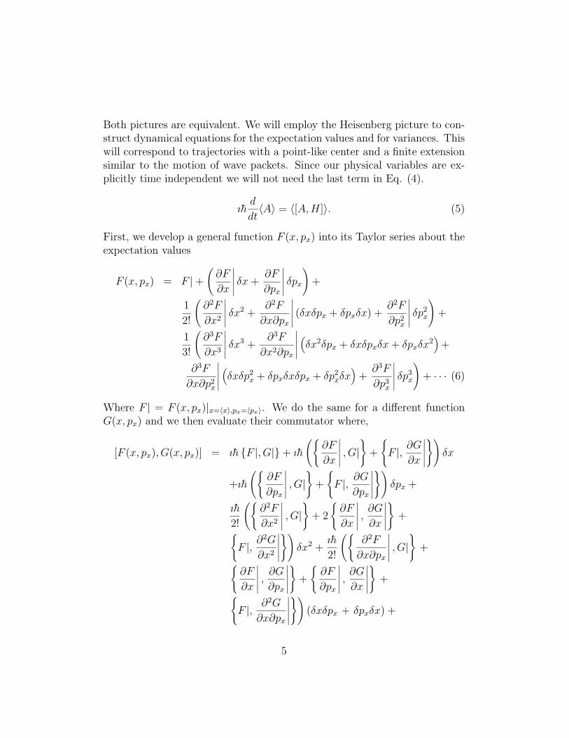
Both pictures are equivalent. We will employ the Heisenberg picture to con-struct dynamical equations for the expectation values and for variances. Thiswill correspond to trajectories with a point-like center and a finite extensionsimilar to the motion of wave packets. Since our physical variables are ex-plicitly time independent we will not need the last term in Eq. (4).

ıhd

dt〈A〉 = 〈[A,H]〉. (5)

First, we develop a general function F (x, px) into its Taylor series about theexpectation values

F (x, px) = F |+(

∂F

∂x

∣∣∣∣∣ δx +∂F

∂px

∣∣∣∣∣ δpx

)+

1

2!

(∂2F

∂x2

∣∣∣∣∣ δx2 +

∂2F

∂x∂px

∣∣∣∣∣ (δxδpx + δpxδx) +∂2F

∂p2x

∣∣∣∣∣ δp2x

)+

1

3!

(∂3F

∂x3

∣∣∣∣∣ δx3 +

∂3F

∂x2∂px

∣∣∣∣∣(δx2δpx + δxδpxδx + δpxδx

2)

+

∂3F

∂x∂p2x

∣∣∣∣∣(δxδp2

x + δpxδxδpx + δp2xδx

)+

∂3F

∂p3x

∣∣∣∣∣ δp3x

)+ · · · (6)

Where F | = F (x, px)|x=〈x〉,px=〈px〉. We do the same for a different functionG(x, px) and we then evaluate their commutator where,

[F (x, px), G(x, px)] = ıh {F |, G|}+ ıh

({∂F

∂x

∣∣∣∣∣ , G|}

+

{F |, ∂G

∂x

∣∣∣∣∣

})δx

+ıh

({∂F

∂px

∣∣∣∣∣ , G|}

+

{F |, ∂G

∂px

∣∣∣∣∣

})δpx +

ıh

2!

({∂2F

∂x2

∣∣∣∣∣ , G|}

+ 2

{∂F

∂x

∣∣∣∣∣ ,∂G

∂x

∣∣∣∣∣

}+

{F |, ∂2G

∂x2

∣∣∣∣∣

})δx2 +

ıh

2!

({∂2F

∂x∂px

∣∣∣∣∣ , G|}

+

{∂F

∂x

∣∣∣∣∣ ,∂G

∂px

∣∣∣∣∣

}+

{∂F

∂px

∣∣∣∣∣ ,∂G

∂x

∣∣∣∣∣

}+

{F |, ∂2G

∂x∂px

∣∣∣∣∣

})(δxδpx + δpxδx) +

5

ıh

2!

({∂2F

∂p2x

∣∣∣∣∣ , G|}

+ 2

{∂F

∂px

∣∣∣∣∣ ,∂G

∂px

∣∣∣∣∣

}+

{F |, ∂2G

∂p2x

∣∣∣∣∣

})δp2

x + · · · (7)

Where {F |, G|} =(

∂F∂x

∣∣∣ ∂G∂px

∣∣∣)−

(∂F∂px

∣∣∣ ∂G∂x

∣∣∣)

represents the Poisson bracket.We now evaluate the expectation value of the commutator and get

〈[F (x, px), G(x, px)]〉 = ıh{F |, G|}+ıh

2!

({∂2F

∂x2

∣∣∣∣∣ , G|}

+ 2

{∂F

∂x

∣∣∣∣∣ ,∂G

∂x

∣∣∣∣∣

}+

{F |, ∂2G

∂x2

∣∣∣∣∣

})〈δx2〉+

ıh

2!

({∂2F

∂x∂px

∣∣∣∣∣ , G|}

+

{∂F

∂x

∣∣∣∣∣ ,∂G

∂px

∣∣∣∣∣

}+

{∂F

∂px

∣∣∣∣∣ ,∂G

∂x

∣∣∣∣∣

}+

{F |, ∂2G

∂x∂px

∣∣∣∣∣

})(〈δxδpx〉+ 〈δpxδx〉) +

ıh

2!

({∂2F

∂p2x

∣∣∣∣∣ , G|}

+ 2

{∂F

∂px

∣∣∣∣∣ ,∂G

∂px

∣∣∣∣∣

}+

{F |, ∂2G

∂p2x

∣∣∣∣∣

})〈δp2

x〉+ · · · (8)

It is difficult to be able to discern where (8) differs from that provided byBatelaan given that it is not fully enumerated in the paper [7].

4 Current Ring Dynamics

In order to develop the Hamiltonian for Brillouin’s thought experiment weneed to find a physical apparatus which fulfills the longitudinal Stern-Gerlachcriterion. Fortunately, a very simple apparatus exits which satisfies all therequirements, it is a circular current loop. The Hamiltonian in cylindricalcoordinates for this apparatus is

H =(pz − Az)

2

2m+

(pρ − Aρ)2

2m+

(pφ − Aφ)2

2mρ2, (9)

6

where Az, Aρ, and Aφ are the vector potentials in cylindrical coordinates.The vector potential is given [8] by Az = Aρ = 0 and

Aφ(r, θ) =4Ia√

a2 + r2 + 2ar sin θ

[(2− k2)K(k)− 2E(k)

k2

], (10)

where r2 = ρ2 + z2 and the argument k of the elliptic integrals K(k) andE(k) is given by

k2 =4ar sin θ

a2 + r2 + 2ar sin θ. (11)

When either a À r, a ¿ r, or θ ¿ 1, then

(2− k2)K(k)− 2E(k)

k2∼= πk2

16. (12)

Within the approximation, Aφ is now

Aφ(ρ, θ, z) ≈ πIa2

c

ρ

(a2 + ρ2 + z2 + 2aρ)32

. (13)

Substituting the values for A into (9) we get

H =p2

z

2m+

p2ρ

2m+

p2φ

2mρ2− ω(z)pφ +

1

2mω(z)2ρ2 (14)

where ω(z) = 12

qB(z)m

and B(z) = ( a√a2+z2 )

3. The fourth term in eq. (14) istwice as large and our fifth term is four times as large as the correspondingterms in the results presented in [7]. The third term also differs from [7]where our p2

φ is replaced by p2φ + 1/4.

5 Dynamical Equations

We now apply Eq. (4) to the dynamical variables that we want to evaluatein order to find the trajectories. Starting with z and pz, we discover that thegeometry of the field environment forces us to look at an increasing numberof expectation values of all the terms that appear in the right hand side ofthe equations that we developed. In order to close the set of equations wetruncated the set at the third order in the small variances. We include aterm o(3) in the equations below to represent the truncation, corresponding

7

to expectation values of the third order and higher (i.e. 〈δp3z〉). Our system

of equations reads nowd〈z〉dt

=〈pz〉m

, (15)

d〈pz〉dt

= − ∂H

∂z

∣∣∣∣∣−1

2

∂3H

∂z3

∣∣∣∣∣ 〈δz2〉 − ∂3H

∂z2∂pφ

∣∣∣∣∣ 〈δzδpφ〉

− 1

2

∂3H

∂z∂ρ2

∣∣∣∣∣ 〈δρ2〉 − ∂3H

∂z2∂ρ

∣∣∣∣∣ 〈δzδρ〉+ o(3), (16)

d〈δz2〉dt

= 2〈δzδpz〉

m, (17)

d〈δzδpz〉dt

=〈δp2

z〉m

− A〈δz2〉 −B〈δzδpφ〉 − C〈δzδρ〉+ o(3), (18)

d〈δp2z〉

dt= −2A〈δzδpz〉 − 2B〈δpzδpφ〉 − 2C〈δpzδρ〉+ o(3), (19)

d〈δzδpφ〉dt

=〈δpzδpφ〉

m, (20)

d〈δzδρ〉dt

=〈δzδpρ〉

m+〈δρδpz〉

m, (21)

d〈δpzδpφ〉dt

= −A〈δzδpφ〉 − B〈δp2φ〉 − C〈δρδpφ〉+ o(3), (22)

d〈δρδpz〉dt

=〈pzδpρ〉

m− A〈δzδρ〉 − B〈δρδpφ〉 − C〈δρ2〉+ o(3), (23)

d〈δzδpρ〉dt

=〈δpzδpρ〉

m− C〈δz2〉 −D〈δzδρ〉 − E〈δzδpφ〉+ o(3), (24)

d〈δp2φ〉

dt= 0, (25)

d〈δρδpφ〉dt

=〈δpρδpφ〉

m, (26)

d〈δρ2〉dt

=〈δρδpρ〉+ 〈δpρδρ〉

m, (27)

d〈δpzδpρ〉dt

= −A〈δzδpρ〉 − B〈δpρδpφ〉 − C〈δρδpρ〉 − C〈δzδpz〉−D〈δρδpz〉 − E〈δpzδpφ〉+ o(3), (28)

8

d〈δρδpρ〉dt

=〈δp2

ρ〉m

− C〈δzδρ〉 −D〈δρ2〉 − E〈δρδpφ〉+ o(3), (29)

d〈δpρδpφ〉dt

= −C〈δzδpφ〉 −D〈δρδpφ〉 − E〈δp2φ〉+ o(3), (30)

d〈δp2ρ〉

dt= −2C〈δzδpρ〉 − 2D〈δρδpρ〉 − 2E〈δpφδpρ〉+ o(3), (31)

d〈φ〉dt

=〈pφ〉

m〈ρ2〉 − 〈ω(z)〉, (32)

d〈pφ〉dt

= 0, (33)

d〈ρ〉dt

=〈pρ〉m

, (34)

d〈pρ〉dt

=〈p2

φ〉m〈ρ3〉 −m〈ω(z)2ρ〉, (35)

with

A =∂2H

∂z2, B =

∂2H

∂z∂pφ

, C =∂2H

∂z∂ρ,D =

∂2H

∂ρ2, E =

∂2H

∂pφ∂ρ. (36)

Those equations whose form has been corrected are (24), (29), and (31).The last term in all three instances was omitted from the original. Thesethree terms are equally important as their preceding terms in each of theirrespective equations because they have the same order of magnitude as eachother term with an evaluated derivative as a coefficient. Also in the definitionof C our ∂ρ replaces the ∂pρ and our ∂pφ replaces the ∂φ from [7].

9

6 Numerical Solutions

6.1 Spin Separation

Most important to the comparison of quantum diffusion and spin separationis the interesting subset of differential equations of motion which describe thelongitudinal motion along z and the widths of the probability distributionsfor the beam. The subset is comprised of equations (15)−(31) and they forma complete set (when truncated to the third order correction). Within thesolution of the time evolution of the beam two variables are very important forthey describe the beam dispersion. These values are 〈δz2〉 which describesthe longitudinal width of the packet and 〈δρ2〉 which is a measure of thetransverse beam width. Splitting will be detectable if splitting, given by

∆zspin =∫ ∫

2azdt′dt =∫ ∫ 2µB

m

∂Bz

∂zdt′dt, (37)

versus dispersion remains reasonable.

6.2 Matlab

This application was chosen for its numerical analysis tools and familiarity.Recently, I had taken a lab class (Physics 430) where I had learned how tosolve similar systems with relative ease in Matlab. The method taught andused is that two M-files are needed, one for the equations, rhs17.m, and onefor the initial conditions of the system and the differential solver,spin.m. Bothrhs17.m and spin.m are available in Appendix B. In solving the system weheld the initial conditions of the apparatus geometry, magnetic field strength,and small quantum correctional uncertainties constant while allowing thebeams macroscopic properties, initial position and momentum, to vary.

10

7 Analysis

7.1 A Typical Result

When the system is evaluated a figure appears, which describes graphicallythe spin separation versus the beam diffusion. If the spin separation linesexit the beam diffusion box, that result indicates the ability to quantitativelymeasure the spin of a free electron. However, if the spin separation lineswere not to exit the beam diffusion box that would correspond to not havingsufficient resolution to separate the diffusion from the separation. Underthe given initial conditions, it appears that the spin separation is unable toovercome the large beam diffusion.

7.2 Possible Improvements

The method appears to be effective at approaching systems that are largelyclassical with a slight quantum correction. The method is appropriate forsystems that are mostly classical. Also a careful determination of optimalinitial conditions needs to be done in order to explore the parameter spaceto find out where spin polarization might be an experimental possibility. Aswe now have it, the mass of the electron, me, the Bohr magneton, µB, andthe charge of the electron, e, are all unitary. Whereas, the beam width (ρ)is five, the current rings radius (R) is 100, and the initial strength of themagnetic field (B0) is ten. This seems inappropriate and can be improved.

8 Conclusion

Although left for history and nearly forgotten, the longitudinal Stern-Gerlachmagnet appears in simulation not to satisfy what Brillouin had hoped; how-ever, a further study with expanded initial conditions should give us a morecomplete view of the validity of Brillouin’s proposal.

11

References

[1] W. Pauli, Collected Scientific Papers, edited by R. Kronig and V. F.Weisskopf (Wiley, New York, 1964), Vol. 2, pp. 544-552.

[2] B. Sundaram and P. W. Milonni, ”Chaos and low-order corrections toclassical mechanics or geometrical optics,” Phys. Rev. E 51, 1971-1982(1995).

[3] N. F. Mott, ”The scattering of fast electrons by atomic nuclei,” Proc.R. Soc. London, Ser. A 124, 425-442 (1929).

[4] W. Pauli, Magnetism (Gauthier-Villars, Brussels, 1930), pp. 183-186,217-226, 275-280.

[5] B. M. Garraway, and S. Stenholm, ”Observing the spin of a free elec-tron,” Phys. Rev. A 60, 63-79 (1999).

[6] L. Brillouin, ”Is it possible to test by a direct experiment the hypothesisof the spinning electron?,” Proc. Natl. Acad. Sci. U.S.A. 14, 755-763(1928).

[7] H. Batelaan, ”Electrons, Stern-Gerlach, and quantum mechanical prop-agation,” Am. J. Phys. 70, 325-331(2002).

[8] W. R. Smythe, Static and Dynamic Electricity (McGraw-Hill, New York,1969), p. 270.

[9] H. Batelaan, T.J. Gay, and J.J. Schwendiman, ”Stern-Gerlach Effect forElectron Beams,” Phys. Rev. Lett. 79, 4517-4521(1997).

12

A Appendices

A.1 3-Dimensional Taylor Expansion for a General Func-tion

F (xi, pi) = F |+(∑

i

∂F

∂xi

∣∣∣∣∣ δxi +∑

i

∂F

∂pi

∣∣∣∣∣ δpi

)+

1

2!

∑

i,j

∂2F

∂xi∂xj

∣∣∣∣∣ δxiδxj

+∑

i,j

∂2F

∂xi∂pj

∣∣∣∣∣ δxiδpj +∑

i,j

∂2F

∂pi∂xj

∣∣∣∣∣ δpiδxj +∑

i,j

∂2F

∂pi∂pj

∣∣∣∣∣ δpiδpj

+1

3!

∑

i,j,k

∂3F

∂xi∂xj∂xk

∣∣∣∣∣ δxiδxjδxk +∑

i,j,k

∂3F

∂xi∂xj∂pk

∣∣∣∣∣ δxiδxjδpk

+∑

i,j,k

∂3F

∂xi∂pj∂xk

∣∣∣∣∣ δxiδpjδxk +∑

i,j,k

∂3F

∂pi∂xj∂xk

∣∣∣∣∣ δpiδxjδxk

+∑

i,j,k

∂3F

∂xi∂pj∂pk

∣∣∣∣∣ δxiδpjδpk +∑

i,j,k

∂3F

∂pi∂xj∂pk

∣∣∣∣∣ δpiδxjδpk

+∑

i,j,k

∂3F

∂pi∂pj∂xk

∣∣∣∣∣ δpiδpjδxk +∑

i,j,k

∂3F

∂pi∂pj∂pk

∣∣∣∣∣ δpiδpjδpk

+ · · · . (38)

A.2 Commutation Relation of Two 3-Dimensional Gen-eral Functions

[F (xi, pi), G(xi, pi)] = ıh∑

i

{F |, G|}+ ıh∑

i

({∂F

∂xi

∣∣∣∣∣ , G|}

δxi

+

{F |, ∂G

∂xi

∣∣∣∣∣

}δxi +

{∂F

∂pi

∣∣∣∣∣ , G|}

δpi

+

{F |, ∂G

∂pi

∣∣∣∣∣

}δpi

)+

ıh

2!

∑

i,j

({∂2F

∂xi∂xj

∣∣∣∣∣ , G|}

δxiδxj

+

{F |, ∂2G

∂xi∂xj

∣∣∣∣∣

}δxiδxj +

{F |, ∂2G

∂xi∂pj

∣∣∣∣∣

}δxiδpj

13

+

{∂2F

∂xi∂pj

∣∣∣∣∣ , G|}

δxiδpj +

{F |, ∂2G

∂pi∂xj

∣∣∣∣∣

}δpiδxj

+

{∂2F

∂pi∂xj

∣∣∣∣∣ , G|}

δpiδxj +

{F |, ∂2G

∂pi∂pj

∣∣∣∣∣

}δpiδpj

+

{∂2F

∂pi∂pj

∣∣∣∣∣ , G|}

δpiδpj

)

+ıh∑

j,k

({∂F

∂xj

∣∣∣∣∣ ,∂G

∂xk

∣∣∣∣∣

}δxjδxk

+

{∂F

∂xj

∣∣∣∣∣ ,∂G

∂pk

∣∣∣∣∣

} (δxjδpk + δpkδxj

2

)

+

{∂F

∂pj

∣∣∣∣∣ ,∂G

∂xk

∣∣∣∣∣

} (δpjδxk + δxkδpj

2

)

+

{∂F

∂pj

∣∣∣∣∣ ,∂G

∂pk

∣∣∣∣∣

}δpjδpk

)+ · · · . (39)

A.3 Expectation Value of the Commutation Relationbetween Two 3-Dimensional General Functions

〈[F (xi, pi), G(xi, pi)]〉 = ıh∑

i

{F |, G|}+ıh

2!

∑

i,j

({∂2F

∂xi∂xj

∣∣∣∣∣ , G|}〈δxiδxj〉

+

{F |, ∂2G

∂xi∂xj

∣∣∣∣∣

}〈δxiδxj〉+

{F |, ∂2G

∂xi∂pj

∣∣∣∣∣

}〈δxiδpj〉

+

{∂2F

∂xi∂pj

∣∣∣∣∣ , G|}〈δxiδpj〉+

{F |, ∂2G

∂pi∂xj

∣∣∣∣∣

}〈δpiδxj〉

+

{∂2F

∂pi∂xj

∣∣∣∣∣ , G|}〈δpiδxj〉+

{F |, ∂2G

∂pi∂pj

∣∣∣∣∣

}〈δpiδpj〉

+

{∂2F

∂pi∂pj

∣∣∣∣∣ , G|}〈δpiδpj〉

)

+ıh∑

j,k

({∂F

∂xj

∣∣∣∣∣ ,∂G

∂xk

∣∣∣∣∣

}〈δxjδxk〉

+

{∂F

∂xj

∣∣∣∣∣ ,∂G

∂pk

∣∣∣∣∣

} (〈δxjδpk〉+ 〈δpkδxj〉2

)

14

+

{∂F

∂pj

∣∣∣∣∣ ,∂G

∂xk

∣∣∣∣∣

} (〈δpjδxk〉+ 〈δxkδpj〉2

)

+

{∂F

∂pj

∣∣∣∣∣ ,∂G

∂pk

∣∣∣∣∣

}〈δpjδpk〉

)+ · · · . (40)

A.4 Running Matlab sources

In order to utilize the code provided below, it is necessary to create the twom-files in the same directory. Then code them as instructed. In order to runthem, you double-click the spin.m file. It will query you as to an appropriateinitial momentum value, enter a value (a reasonable value might be 100-1500), and it will provide the results for that value. Built into the code isa disallowance for the abrogation of the physical laws of nature (i.e. whenthe outputs of the code violate the Heisenberg Uncertainty Principle the codequits).In the figures that pop up after successfully running the code, the axesrepresent the longitudinal axis of the longitudinal Stern-Gerlach magnet (i.e.current ring).

A.5 Source 1: rhs17.m

function F=rhs18(t,y)

global m;

global pphi;

global rho;

global Bo;

global R;

global q;

w=q*Bo/2/m*(R/(R^2+y(1)^2)^(1/2)))^3;

w1=-(3/2)*q*Bo/m*R^3*y(1)/((R^2+y(1)^2)^(5/2));

w2=-(3/2)*q*Bo*R^3/m*(R^2-4*y(1)^2)/((R^2+y(1)^2)^(7/2);

w3=(15/2)*q*Bo*R^3/m*y(1)*(3*R^2-4*y(1)^2)/((R^2+y(1)^2)^(9/2));

Hz1=-pphi*w1+m*w*w1*rho^2;

Hz3=-pphi*w3+3*m*w1*w2*rho^2+m*w*w3*rho^2;

Hz2p_phi=-w2;

Hzrho2=2*m*w*w1;

Hz2rho=2*m*w1^2*rho+2*m*w*w2*rho;

A=-pphi*w2+m*w1^2*rho^2+m*w*w2*rho^2;

15

B=-w1;

C=2*m*w*w1*rho;

D=3*pphi^2/m/(rho^4)+m*w^2;

E=-2*pphi/m/(rho^3);

F=zeros(length(y),1);

F(1)=y(2)/m;

F(2)=-Hz1-(1/2)*Hz3*y(3)-Hz2pphi*y(6)-(1/2)*Hzrho2*y(13)-Hz2rho*y(7);

F(3)=2*y(4)/m;

F(4)=y(5)/m-A*y(3)-b*y(6)-C*y(7);

F(5)=-2*A*y(4)-2*B*y(8)-2*C*y(14);

F(6)=y(8)/m;

F(7)=y(10)/m+y(14)/m;

F(8)=-A*y(6)-B*y(11)-C*y(12);

F(9)=y(14)/m-A*y(7)-B*y(12)-C*y(13);

F(10)=y(14)/m-C*y(3)-D*y(7)-E*y(6);

F(11)=0;

F(12)=y(16)/m;

F(13)=y(15)/m;

F(14)=-A*y(10)-B*y(16)-c*y(15)-C*y(4)-D*y(9)-E*y(8);

F(15)=y(17)/m-C*y(7)-D*y(13)-E*y(11);

F(16)=-C*y(6)-D*y(12)-E*y(11);

F(17)=-2*C*y(10)-2*D*y(15);

A.6 Source 2: spin.m

clear;close all;

global m;

global pphi;

global rho;

global Bo;

global R;

global q;

initial conditions

m=1;pphi=0;rho=5;Bo=10;R=100;q=1;mu=1;

y0=zeros(17,1);

y0(1)=-500;

16

y0(2)=input(’ initial momentum - ’);

y0(3)=1;

y0(4)=1;

y0(5)=1;

y0(6)=1;

y0(7)=1;

y0(8)=1;

y0(9)=1;

y0(10)=1;

y0(11)=0;

y0(12)=1;

y0(13)=1;

y0(14)=1;

y0(15)=1;

y0(16)=1;

y0(17)=1;

options=odeset(’RelTol’,1e-8);

tstart=0;tfinal=10;

N=1024;

taue=(tfinal-tstart)/(N-1);

te=tstart:taue:tfinal;

[t,y]=ode45(@rhs_17,te,y0,options);

spin separation animation

h1=0:.002:.15;

h2=0:.005:.15;

for n=1:N-1

spin down (backward)

xdown(1)=y0(1);

vdown(1)=y0(2)/m;

adown(1)=(mu/m)*(-3*Bo*R^3)*xdown(1)/((R^2+(xdown(1))^2)^(5/2));

vdown(n+1)=vdown(n)+adown(n)*taue;

xdown(n+1)=xdown(n)+vdown(n)*taue+(1/2)*adown(n)*(taue)^2;

17

adown(n+1)=(mu/m)*(-3*Bo*R^3)*xdown(n+1)/((R^2+(xdown(n+1))^2)^(5/2));

no spin

xzero(1)=y0(1);

vzero(1)=y0(2)/m;

azero(1)=0;

vzero(n+1)=vzero(n)+azero(n)*taue;

xzero(n+1)=xzero(n)+vzero(n)*taue+(1/2)*azero(n)*(taue)^2;

azero(n+1)=0;

spin up (forward)

xup(1)=y0(1);

vup(1)=y0(2)/m;

aup(1)=(mu/m)*(3*Bo*R^3)*xup(1)/((R^2+(xup(1))^2)^(5/2));

vup(n+1)=vup(n)+aup(n)*taue;

xup(n+1)=xup(n)+vup(n)*taue+(1/2)*aup(n)*(taue)^2;

aup(n+1)=(mu/m)*(3*Bo*R^3)*xup(n+1)/((R^2+(xup(n+1))^2)^(5/2));

end

square wave animation & blurring

n=0;

set(gca,’NextPlot’,’replacechildren’)

for j=1:32:N

mu=y(j,1);

sigma=y(j,3);

delta=y(j,5);

if sigma<0

fprintf(’ position dispersion violation \%g \n’,y(j,3));

break

elseif delta<0

fprintf(’ momentum dispersion violation \%g \n’,y(j,5));

break

elseif delta*sigma<.25

fprintf(’ heisenberg uncertainty violation \%g \n’,y(j,5)*y(j,3));

break

else

if sigma>250

18

sigma=250;

end

x=(mu-sigma):(mu+sigma);

s=1/2/sigma;

a=0:.0005:s;

plot(x,s,’k-’,mu-sigma,a,’k-’,mu+sigma,a,’k-’,xdown(j),h2,’b-’,xup(j),h1,’r-’);

axis([y(j,1)-150 y(j,1)+150 0 .15])

n=n+1;

Q(:,n)=getframe;

end

end

movie(Q,0)

19