The Causal Effect of Competition on Prices and Quality:

Evidence from a Field Experiment1

Matias Busso Sebastian Galiani

Research Department

Inter-American

Development Bank

Department of Economics

University of Maryland

February 2015

Abstract

This paper provides the first experimental evidence on the effect of increased

competition on the prices and quality of goods. We rely on an intervention that

randomized the entry of 61 retail firms (grocery stores) into 72 local markets in the

context of a conditional cash transfer program that serves the poor in the

Dominican Republic. Six months after the intervention, product prices in the

treated areas had decreased by about 6%, while product quality and service quality

had not changed. Our results are also informative for the design of social policies.

They suggest that policymakers should pay attention to supply conditions even

when the policies in question will only affect the demand side of the market.

JEL: D4, L1, I3.

Keywords: Competition, prices, quality, experimental evidence, design of social

policies.

1 Acknowledgements: We thank Francisca Müller, Juan Sebastian Muñoz and Dario Romero Fonseca for their

excellent project management and research assistance. We are grateful for the very useful comments made by

Daron Acemoglu, Alberto Chong, Gary Libecap, James Poterba, Ernesto Schargrodsky, Gustavo Torrens and

participants at various seminars. We also thank the valuable collaboration and feedback provided during the

early stages of the project by Van Elder Espinal, Mayra Guzman, Carlos Leal and Mario Alberto Sanchez.

This experiment has been registered with the American Economic Association RCT Registry under number

AEARCTR-0000343. The views expressed herein are those of the authors and should not be attributed to the

Inter-American Development Bank.

1

1. Introduction

Ever since Adam Smith, economists have seen market competition as a way of achieving

economic efficiency. If a competitive equilibrium exists, then the equilibrium is necessarily

Pareto optimal in the sense that there is no other allocation of resources which would make

all participants in the market better off. Adam Smith considered competition to be a form of

rivalry between suppliers that eliminated excessive profits, did away with excessive supply

and satisfied existing demand (Stigler, 1957). Competition also exerts downward pressure

on costs, reduces slack periods and provides incentives for the efficient organization of

production (Nickell, 1996). Price-taking implies that no supplier is able to exert market

power, which means that firms do not price profitably above the marginal cost of

production and that consumer surplus is therefore maximized. All these sound arguments

notwithstanding, real-world experimental evidence on the welfare effects of competition

has not, to the best of our knowledge, been presented.

In this paper we exploit a randomized control experiment to assess what impact the entry of

new grocery stores into a given market has on prices, product quality (as defined by product

brands and varieties) and service quality. The experiment was part of an attempt to improve

the operations of the Dominican Republic’s Solidaridad conditional cash transfer program.

This program provides monetary transfers to poor families that can only be used by means

of a debit card which is accepted only by a network of grocery stores that are affiliated with

the program. The program beneficiaries represent a large share of these stores’ customers

and sales.

Only a certain number of stores are authorized to accept the program’s debit cards. Because

entry into this market is restricted by the program design, these retail stores can potentially

wield market power. The government argued that they were using their market power to

raise prices and to offer a more limited range of products than those offered by stores

outside the network. This was seen as signaling a loss of consumer surplus and therefore a

potential welfare loss. In response to this situation, we worked with the Dominican

government to determine the extent to which the expansion of the retail network might fuel

competition. The intervention was conducted during May and June 2011 and involved

bringing 61 new grocery stores into the network in 72 districts. The experimental design

allowed anywhere from zero to three stores to begin operating in each district.

We use data on both retail stores and households located in the areas concerned which was

collected at baseline and six months after the intervention. Our data allow us to arrive at

precise price measurements which we can then use to infer quality. The surveys also

incorporate other independent measures of quality. We estimate average treatment effects

using the randomization assignment in order to instrument the potentially endogenous entry

of new stores induced by noncompliance with randomization.

2

We find that entry into the market leads to a significant and robust reduction in prices but

that it does not lead to any change in the quality of the products or service (delivery of

those goods) provided by the grocery stores. We also impose some structure in order to

estimate the price-elasticity at entry, which we find to be 0.06.

Previous work analyzing the effects of competition has relied on observational data.

Trapani and Oslon (1982) analyze the effect of the deregulation of the airline industry in

the US on the price and quality of service by studying the relationship between fare level,

open entry and service quality. This analysis exploits a cross-sectional sample of 70

markets within the United States in 1971 and 1977. The authors found that increasing

competition in the airline industry leads to a reduction both in prices and in the average

quality of service. Their paper shows that the independent effect of decreasing market

concentration, which leads to a higher quality of service, is overshadowed by the

independent effect of price competition (lower prices), which, in turn, lowers the quality of

service. Bresnahan and Reiss (1990) study the interrelationships among potential entrants’

profit levels and decisions using cross-sectional data on 149 geographically isolated US

markets for new automobiles. They estimate that the second entrant has nearly the same

costs and market opportunities as the first entrant. They also find that entry does not cause

price-cost margins to fall by a significant amount. Bresnashan and Reiss (1991) examine

the prices of tires in the United States to determine at what point further entry does not lead

to any further price decrease, which the authors point out would be evidence that market

competition had been achieved. Their study suggests that four retailers would be sufficient

for the tire market to be (effectively) competitive.2 Goolsbee and Syverson (2008) study the

entry of a low-price competitor (Southwest Airlines) into the airline industry in the US.

They find that large price decreases occur during the first three quarters of the time period

that elapses between the announcement of entry and the point in time when actual entry

occurs.

Several papers have developed econometric models to estimate the effects of market entry,

including those of Carlton (1983), Berry (1992), Bresnahan and Reiss (1989), Bresnahan

and Reiss (1991) and Reiss and Spiller (1989). Geroski (1989) examines a dynamic

feedback model of entry and profit margins applied to panel data covering a six-year period

(1974-1979) for 85 three-digit industries in the United Kingdom. He finds that entry

barriers are rather high in most industries and that there are noticeable differences in the

pace of competitive dynamics.

Besker and Noel (2009) analyze the effect of Wal-Mart’s entry into the grocery market

using a store-level price panel dataset. They find that competitors’ response to the entry of a

Wal-Mart store, which has a price advantage over competitors of about 10%, is a price

2 Dufwenberg and Gneezy (2000) set up a lab experiment to address this question. They designed an

experiment in which the model resembles an oligopolistic market with homogenous products and find that

four competitors were sufficient to drive the equilibrium toward the competitive outcome.

3

reduction of 1%-1.2%, on average, with most of this reduction being accounted for by

smaller-scale competitors. They conclude that competitors’ responses vary in line with their

degree of differentiation from Wal-Mart. At one extreme, the largest supermarket chains

reduce their prices by less than half as much as smaller competitors. At the opposite

extreme, low-end grocery stores, which compete more directly with Wal-Mart, cut their

prices by more than twice as much as higher-end stores. Jia (2008) develops an empirical

model –one which relaxes the assumption that entry into different markets is independent—

to assess the impact of Kmart stores on Wal-Mart stores and other discount retailers and to

quantify the size of the scale economies obtained within a given chain. She finds that the

negative impact of Kmart’s presence on Wal-Mart’s profits was much stronger in 1988 than

in 1997, while the opposite is true for the effect of Wal-Mart’s presence on Kmart’s profits.

In a more recent paper, Bennett and Yin (2013) explore the relationship between market

development and drug quality by evaluating the impact of chain-store (Med-Plus) entry into

the Indian pharmaceutical industry. They rely on a quasi-experimental variation and exploit

a difference-in-differences identification strategy and find that the entry of a chain store

leads to a relative 5% improvement in quality, measured on the basis of compliance with

the standards of the Indian Pharmacopeia Commission, and a 2% decrease in prices. The

authors conclude that the chain store increases retail competition by offering higher-quality

drugs and lower prices. Although this evidence is compelling and very interesting, the

effects associated with chain-store entry cannot be unequivocally attributed to an increase

in competition, since the new stores operate on the basis of a completely different rationale

than the incumbent family-run stores do. As the authors argue, it is better to interpret the

evidence that they have gathered as also being indicative of the effects of market

development in a developing country.

Although several important studies have used different setups to focus on the effects of the

entry of new competitors into imperfectly competitive markets, our paper contributes to the

literature by reporting on what is, to the best of our knowledge, the first randomized-

controlled field experiment designed to assess the impact of increasing competition on

prices and quality. Without neglecting the very important role of theory in the analysis of

the data provided by previous works (see, among others, Einav and Levin (2010)), this is a

significant contribution because, as has been acknowledged in the literature, competition in

non-experimental studies is likely to be endogenous for the parameters of interest (see,

among others, Blundell et al. (1999) and Aghion et al. (2014)).

Our paper addresses a fundamental question in economics. It exploits experimental

variability in the entry of existing stores into a segment of a market where entry is

constrained. The results do, in fact, indicate that our experiment induces a large and

exogenous increase in competition among retail stores in that market segment. Naturally,

even though our findings, in conjunction with economic theory, provide an outline of the

4

general principles that are in play, as in the case of any study on a given market, it may not

be possible to directly extrapolate our conclusions to other industries or populations.

The remainder of this paper is organized as follows. Section 2 presents a simple model that

is used to guide the empirical analysis. Section 3 describes the setting in which the

intervention took place. Section 4 discusses the experimental design. Section 5 presents the

data used in this study. In Section 6, we present our empirical strategy. In Section 7, we

present the empirical results. Section 8 concludes.

2. A Simple Model

Theoretical models of imperfect competition make various predictions about the

competitive effects of market entry. Firms with market power may exploit their position to

lower quality, just as they may raise prices (Tirole, 1988). Competition attenuates the

incentive to do so and prompts firms to increase quality and/or decrease prices.

In most models, the entry of new competitors leads to price reductions by putting more

competitive pressure on market incumbents. This is a prediction of most standard

imperfect-competition models, such as differentiated-product Bertrand competition and

spatial-competition models, as well as of many models with equilibrium price dispersion

(such as that of Reinganum, 1979).

The effect of competition on product quality has been shown to be less clear-cut across the

various models. Greater market power prompts firms to exploit their position in order to

increase prices and reduce quality. Competition attenuates the incentives to do so; however,

firms are likely to compete through quality if quality improvements translate directly into

greater demand. The effect of competition on quality depends on the extent to which

consumers perceive quality. Dranove and Satterthwaite (1992) explore the relationship

between competition and quality by varying the precision of price and quality signals in a

search model. They find that competition has an effect on quality when consumers have

received quality signals that are at least somewhat informative.

We rely on a simple Cournot model of competition where n firms compete in price and

quality. We impose a reasonable set of assumptions in relation to the experiment that we

analyze in this paper and derive results for the effect of competition on both the price of the

product supplied and the quality of the service provided.

We view the market that we are studying here as one that, in the absence of market entry

restrictions, would operate much like a monopolistic competitive market, where retailers

would differ mostly in terms of their location and, to some extent, the quality of the service

provided. In our experiment retail stores offer a similar set of goods, but they can alter the

varieties/brands they offer (the perceived product quality) and they can also vary the range

5

of varieties/brands thus offering a different quality of service. They can also vary the

customer service, another dimension of the quality of service provided.

In this section, in order to keep the model simple, we will abstract from the selection of

multiple products/varieties and will consider firms that face a downward demand curve for

a homogenous product in an oligopolistic market in which entry barriers enhance the

market power of the incumbent retailers. Those retailers have also chosen the overall

quality of the service they supply (which we model as one-dimensional). In the empirical

analysis, we will seek to determine whether firms change the varieties/brands of the

products they offer. In other words, we will try to establish whether, as a result of more

competition, they provide products of a different quality at the same price or whether they

offer products of the same quality at a lower price (or a combination of the two).

Assume that there are n identical firms that compete in a market of differentiated goods and

that they choose the quantity of a homogenous product (𝑞𝑖) that is produced and the quality

of the service provided (𝑣𝑖). We will suppose that the residual inverse demand curve that a

firm faces is separable in terms of quantity and quality and that it depends not only on the

quantity supplied by other firms, but also on the difference between the quality of the

service provided by that firm and the service quality offered by the rest of the firms in that

market, as follows:

𝑝𝑖 = 𝐹(𝑣𝑖 − 𝛼∑ 𝑣𝑗𝑗≠𝑖 ) − 𝛽𝑞𝑖 − 𝛿 ∑ 𝑞𝑗𝑗≠𝑖 (1)

where 𝐹 is a strictly increasing function and 𝛼 is such that the argument in 𝐹 is always

positive. Note that the lower the value of 𝛿, the lower the degree of substitution between

products. Similarly, the lower the value of 𝛼, the lower the degree of substitution between

service qualities. At the limit, if both 𝛼 and 𝛿 were zero, then increasing competition would

not affect firm behavior.

For the sake of simplicity, we assume that there is no fixed cost and that the cost function is

linear in the amount produced, but that it is increasing and convex in the level of quality

supplied. This may reflect the fact that the initial increases in quality can be achieved by

means of minor adjustments or improvements in inputs, while further improvements in

quality are more costly. The cost function is then:

𝑐𝑖(𝑞𝑖 , 𝑣𝑖) = 𝑐𝑞𝑞𝑖 + 𝑐𝑣(𝑣𝑖)

2

2

Using both the inverse demand curve and the cost function, we can write the profit function

of a firm i as:

𝜋𝑖 = [𝐹(𝑣𝑖 − 𝛼∑ 𝑣𝑗𝑗≠𝑖 ) − 𝛽𝑞𝑖 − 𝛿 ∑ 𝑞𝑗𝑗≠𝑖 ]𝑞𝑖 − 𝑐𝑞𝑞𝑖 − 𝑐𝑣(𝑣𝑖)

2

2

6

The problem that the firm faces is then:

max𝑞𝑖;𝑣𝑖

𝜋𝑖

The first-order conditions for this optimization problem are then:

𝜕𝜋𝑖𝜕𝑞𝑖

= [𝐹 (𝑣𝑖 − 𝛼∑𝑣𝑗𝑗≠𝑖

) − 2𝛽𝑞𝑖 − 𝛿∑𝑞𝑗𝑗≠𝑖

] − 𝑐𝑞 = 0

𝜕𝜋𝑖𝜕𝑣𝑖

= 𝐹′(𝑣𝑖 − 𝛼∑𝑣𝑗𝑗≠𝑖

)𝑞𝑖 − 𝑐𝑣𝑣𝑖 = 0

If a symmetric Nash equilibrium exists such that (𝑝𝑖, 𝑞𝑖 , 𝑣𝑖) = (𝑝, 𝑞, 𝑣) for all firms, then

the previous two equations become:

𝐹(𝑣[1 − 𝛼(𝑛 − 1)]) − [2𝛽 + 𝛿(𝑛 − 1)]𝑞 = 𝑐𝑞

𝐹′(𝑣[1 − 𝛼(𝑛 − 1)])𝑞 = 𝑐𝑣𝑣

We now use this model to investigate how the number of firms in the market affects the

equilibrium values of the quantity offered and the quality chosen by each firm. If 𝐹 is

concave, which we will assume it is, it then follows that 𝑑𝑣

𝑑𝑛> 0 and

𝑑𝑞

𝑑𝑛< 0. In other words,

as the number of firms in the market increases, the amount of the product sold by each firm

in the symmetric equilibrium decreases, while product quality rises. To see how the

equilibrium price reacts to entry, we then turn to equation (1) and replace the arguments

with their equilibrium values:

𝑝 = 𝐹([1 − 𝛼(𝑛 − 1)]𝑣) − [𝛽 + 𝛿(𝑛 − 1)]𝑞

If we differentiate this expression with respect to n, we easily find that 𝑑𝑝

𝑑𝑛< 0. This means

that the effect of increased competition in the symmetric equilibrium is a reduction of

prices.

Thus, if customers value the increase in quality, then firms, in a symmetric Nash

equilibrium, will react to an exogenous increase in the number of firms by reducing prices

and increasing quality. If, instead, customers do not value quality (F’= 0), firms will

compete only on price, as is the case in the Cournot model.

7

3. Setting

Our study exploits the design and implementation of a conditional cash transfer (CCT)

program in the Dominican Republic. CCT programs have been extensively used since the

mid-1990s as one of the main tools for providing social protection to people in low- and

middle-income developing countries. The Dominican Republic introduced the Solidaridad

CCT program in 2005.

The program provides monetary transfers to families living in poverty. Eligibility is

determined on the basis of a quality-of-life score that is used to classify households into

different socioeconomic groups. All households identified as extremely-to-moderately poor

are eligible. In 2005 the program initially reached about 200,000 households. It then

underwent two big expansions: one in 2007 (when it reached 460,000 households) and

another in 2010 (when its coverage expanded to 520,000 households).3 In the interim

periods, the number of beneficiaries stayed relatively constant. During 2011, the year of our

study, the program had reached a plateau, with the number of program beneficiaries

increasing by around 3% during the year.

This CCT program includes two components. First, a health component (“Comer es

Primero”/ “Eating comes First”) provides households with a transfer of about US$ 19.5 per

month.4 Transfers are contingent on parents bringing those of their children who are under

five years of age to the community health center on a regular basis for developmental

monitoring and immunizations. In addition, they are expected to attend workshops that

provide instruction in nutrition, family planning, self-care and hygiene. The program’s

second component focuses on education (“Incentivo a la Asistencia Escolar”/ “Incentives

for School Attendance”) and transfers a given amount of money to households depending

on the composition of the family: Households with one or two eligible children (aged 6-16)

receive US$ 8.4 per month; those with three children receive US$ 12.5; and those with four

or more children receive US$ 16.7 per month. Transfers are contingent on school

enrollment and attendance of children between 6 and 16 years of age.5 The typical

household (three children of school age) would receive a total transfer of US$ 36, which

represents 17% of the median monthly food expenditure of the target population.6

Households’ monetary transfers are deposited into individual bank accounts. More

importantly, in order to ensure that the transfer is spent on food, the money cannot be

3 Expanding coverage is costly, since the government has to conduct a population census in poor areas in

order to determine household eligibility. 4 Based on a 2010 exchange rate of DR$ 35.9 to the dollar. 5 Students must not repeat a grade more than once and must have an 85% attendance record, as a minimum. 6 In principle, households might receive other money transfers that are deposited in their bank accounts, such

as a subsidy for higher education (“Incentivo a la educación superior”), a pension for the elderly living in

extreme poverty (“Programa de protección a la vejez en pobreza extrema”), a subsidy to buy gas

(“Bonogas”) and/or a subsidy to pay the electricity bill (“Bonoluz”). Some of these transfers could be used in

the same retailers that are under analysis here.

8

withdrawn from the bank but, instead, can only be spent by using a debit card7 that works

only in a network of program-affiliated retailers (the network is known as the “Red de

Abastecimiento Social” / “Social Supply Network”), most of which are grocery stores. This

network of retailers and its interaction with program beneficiaries (the stores’ customers)

play a central role in this study.

There is a standardized procedure for joining the network.8 First, the government executing

agency9 regularly opens calls for applications in certain districts and, via a community

liaison, distributes application forms and encourages local stores to apply. Second,

interested retailers fill in and submit the application. Third, the application is reviewed and

checked by the executing agency. Inspectors visit the stores and record information on the

applicants’ infrastructure and access to basic services, including a phone line – a potentially

costly item for the stores, but one that is necessary in order for the debit card or magnetic

stripe reader to operate. Finally, scores are assigned to the applications and stores are

allowed to join the network or not, depending on their score and on the number of affiliated

stores already in the district in question.

Prima facie, this application procedure is cost-free for retailers. However, entering the

network can still be costly for two reasons. First, many of these stores operate informally.

The application requires them to provide a tax identification number and to have a bank

account, which increases the (perceived) probability of being audited. Second, some

retailers may be asked to do some upgrading, which could involve buying a card reader,

connecting to a phone line, having a power generator and satisfying some minimum

sanitary conditions.

The retailer’s payoff for participating in the network may be a larger sales volume and

higher profits, if the retailer enjoys some market power. In fact, in 2005, at the outset of the

program, it was unclear to many retailers what the benefits of participating in the network

might be. It was not yet clear how many CCT program beneficiaries (i.e. these stores’

customers) there would be or how many nearby competitor retailers would be in the

network. As a consequence, only a few retailers applied for entry in 2005. As a way of

making affiliation attractive to retailers, the authorities decided to limit the number of stores

that could join the network based on the number of beneficiaries in each district. In many

districts, this effectively gave local market power to some retailers. In fact, the executing

agency discovered that some stores had increased their prices and were offering a more

limited variety of products than stores outside the network.10

7 This debit card can be used only by the head of household. 8 The standard process of affiliation and the operation of the retail network are governed by a set of

administrative rules detailed in “Reglamento de Funcionamiento de la Red de Abasto Social” from ADESS. 9 The Social Subsidies Administration (Administradora de Subsidios Sociales (ADESS)). 10 See the report by ADESS entitled “Proyecto de Ampliación de la Red de Abasto Social” (pp.11-13).

9

In our setting, market entry means that a store is allowed to sell to program beneficiaries in

the relevant district. Retailers entering the program network (entrants) were already

operating in the non-CCT market. Entrants are very similar to retailers already affiliated

with the program (incumbents). They sell products of similar quality at similar prices, and

the stores’ characteristics are also similar. The only meaningful difference is that the

entrants are smaller, as they have, on average, about 12% fewer sales and 11% fewer

employees than incumbents.

Table 1 presents some descriptive statistics on both customers and retailers in the areas

under study. There are several important facts we would like to highlight.

Retailers are small, owner-run “mom-and-pop” shops. They sell mainly non-perishable

food products and typically supply a very limited number of fresh products (fruits,

vegetables or dairy products). This is partly due to storage limitations and partly to the

types of goods that the population in these areas consumes. In fact, 75% of the total amount

spent on food by consumers in these areas is spent on non-perishable goods.11

The people who shop in the areas under study are typically poor, with their earnings being

equivalent to slightly more than one quarter of the country’s per capita GDP. As is typical

in many Latin American countries, residential segregation is prevalent in the Dominican

Republic, with poor households clustered in different areas than middle- and high-income

households (Bouillon, 2012). Thus, the markets under analysis are segmented by income,

and most of the households whose members shop in the retail stores that we are analyzing

are poor. Within these markets, from the retailers’ point of view, the only difference

between program beneficiaries and non-beneficiaries is the usage of the CCT debit card.12

Beneficiaries shop during regular business hours. In incumbent stores, program

beneficiaries can use the CCT transfer money to purchase only food products (of any brand

or variety). A few items, such as alcoholic beverages and tobacco products, are specifically

excluded from purchases made with the debit card, although, naturally, they could be

bought by program beneficiaries if they pay for those products with cash. 13

CCT beneficiaries represent a large share of the market for these retailers. Using

information on sales, on the number of beneficiaries in the areas under study and on the

program transfers, we estimate that about 56% of these retailers’ sales are financed directly

by the CCT transfers. However, when program beneficiaries shop in these stores, they buy

11 For this reason, in our analysis we focus on a limited set of products that capture about 85% of this set of

non-perishable goods. See the Appendix I for more details about the types of goods under analysis. 12 Simply being poor is not sufficient to make a person eligible for the program. People also need to prove that

they are citizens of the Dominican Republic. It is estimated that 30% of households whose members are living

in extreme poverty lack the proper documentation to be eligible for social programs. 13 The CCT executing agency drew up a list of products that cannot be sold to beneficiaries using the debit

card (e.g., alcohol). The CCT program regulations also explicitly prohibit fictitious transactions in exchange

for cash.

10

products both with the CCT debit card and with cash. Because they typically shop in only

one store on any given day, since the transaction costs of going to more than one shop are

high, a store’s membership in the CCT retail network provides it with some measure of

market power. Using information on food expenditure, and assuming that all spending on

groceries is done within the district where the members of the household live, we estimate

that as much as 96% of an incumbent’s sales could potentially come from program

beneficiaries. The importance of program beneficiaries for these retailers is also confirmed

by self-reported measures: 96% of retailers located in the areas under study and currently in

the network (incumbents) claim that being affiliated with the CCT program has increased

their sales.

The data suggests that there is room for local market power and for price discrimination.

Program beneficiaries’ mobility is limited: only 15% of them own a car or a motorcycle

and, as a consequence, 95% of them shop only in a retailer in the program network located

within 10 blocks of their house. As a consequence, retailers can potentially wield local

market power. In the smaller shops, items are placed on shelves located behind the counter

while, in the larger establishments, items are on shelves that can be browsed by the

customer. The prices of the different items are not always in plain view. Only about 41% of

retailers have prices posted where the customer can see them. Although we do not have

direct evidence of it, this setup seems to provide an opportunity for third-degree price

discrimination, since, because retailers know that certain customers are CCT beneficiaries

who will be paying with a debit card, the retailers could charge them a different price. In

fact, only 44% of retailers stated that they never bargain over prices with their customers.

Despite the beneficiary population’s low degree of mobility, the market could be much

more competitive if the government’s entry restrictions were not in place. Almost 95% of

customers could identify a non-affiliated store within a 10-block radius from their house.

These potential entrant stores are very similar to the incumbent stores and have entered

freely into the non-CCT market, which is a more competitive environment.14

4. Experimental Design

The particular context in which the network of retailers operates has been a cause of

concern for the government. The market power wielded by the stores belonging to the

network allows them to increase prices and to offer a more limited variety of products than

stores outside the network. This implies a loss of consumer surplus and therefore a potential

welfare loss. In addition, over time the CCT program has been increasing the number of

beneficiaries, which exacerbates these problems. In response to this situation, the

authorities have designed a plan for the expansion of the retail network. The goals of the

14 See Appendix Table A1.

11

plan are to address the needs of all the beneficiary clientele of each store and encourage

competition among those stores in order to increase the effectiveness of the subsidies

awarded under the program.

In this context we worked with the CCT executing agency and the Inter-American

Development Bank (IDB) to propose a way of expanding the network as a possible means

of responding to the concerns raised by the government of the Dominican Republic. We

proposed and designed an experimental evaluation. The actual implementation of the

experiment was the responsibility of the CCT executing agency based on guidelines

provided by the IDB.

The intervention consists of an exogenous randomized increase in the number of retailers

associated with the network across districts.15

We use this randomized variability in the

entry of new retail stores into the network servicing the CCT beneficiaries as a means of

evaluating the effect of an increase in competition on prices, product quality and retail

service quality.

The districts used in this experiment were identified by the CCT executing agency with two

considerations in mind. First, there needed to be, before treatment, a relatively strong

demand for consumption goods per retailer and, second, it had to be feasible, at least a

priori, to expand the number of stores in the district. Relatively high-demand districts were

defined as those expected to have more than 100 program beneficiaries per retailer. in order

to increase the possibilities of expanding the product supply by recruiting new retailers, it

was decided that the districts should be located in municipalities with a population of over

15,000 in which at least 30% of the population was urban. In addition, they had to have at

least one non-affiliated retailer that would be interested in joining the network. Ultimately,

72 districts were included in the experiment. The intervention was implemented in three

stages.

First, before randomization, between December 2010 and May of 2011, the CCT executing

agency collected applications from retailers that wanted to become part of the network.

Each one of the 72 districts was built up starting from a targeted neighborhood that was in

an area in which the executing agency was particularly interested in expanding the retail

network. The aim was to have at least three candidates for entry in each neighborhood.

However, as it turned out, this was not always possible, either because there were not

enough applicants or because some of the applicants were not eligible. Eligibility was

assessed by the executing agency on the basis of visits to the stores and store audits. In

those cases in which the search for potential entrants yielded few feasible candidates, the

15 The National Statistics Office divides the country into provinces, municipalities, sections and

neighborhoods. This classification was being used by the CCT executing agency and, to simplify the project’s

implementation, the evaluation was based on that same convention. Districts are composed of either one

neighborhood or two adjacent neighborhoods.

12

executing agency expanded the search area to include nearby areas (which we will refer to

as “non-targeted neighborhoods”). The search for candidates was undertaken in all the

neighborhoods covered by the study. Non-targeted neighborhoods were adjacent to targeted

areas and were also places in which, according to administrative data, program

beneficiaries went to do their shopping. Given the way in which they were defined, these

districts are akin to local markets. The 72 selected districts were then used to provide the

framework for randomization.

Table 2 presents statistics that provide an overview of the distribution of distances between

retailers within districts and the distances between districts (computed using pre-

intervention data). 16

The median distance between retailers within districts was about 246

meters, and the median distance between districts was approximately 3.4 kilometers.

Within the corresponding provinces, the districts were far apart.

Each district was then assigned a random number in the set {0, 1, 2, 3}. This defined the

number of potential new entrant retailers that the executing agency would try to recruit.

Actual affiliation could, in principle, differ from the intended/randomized affiliation

because of a shortage of eligible applicants for entry into the network (noncompliance).

Another source of noncompliance could be a failure on the part of the CCT executing

agency to follow the intervention protocol.17

Table 3 shows that, before treatment, there were some 341 retailers operating in the

network within these 72 districts. Under full compliance, the design was such that a total of

99 new retailers would enter the network, which would represent an intended increase of

29% in the number of stores. A total of 21 districts were randomized to receive no entry of

new retailers (non-intention-to-treat districts), while 51 districts were randomized {1, 2, or

3} for retailers to enter the network (intention-to-treat districts).

Affiliation occurred as indicated in the protocol. When the number of eligible applicants

was less than or equal to the number of randomized new entrants, all of them were

affiliated with the network. In those cases in which the number of applicants was larger

than the number assigned by randomization, the entrants were selected randomly from

among the eligible stores. The actual enrollment in the network was carried out in May-

June 2011 by the executing agency using a standardized procedure.

Table 4 describes randomized and actual entry. A total of 61 retailers entered the network

in these districts, thereby increasing the number of retailers operating in these markets by

26% in the treated areas. In 38 districts (53%), randomization was achieved (perfect

16 Even though we collected information on the location of the retailers in our sample, the National Statistics

Office of the Dominican Republic does not have the type of information that would be needed in order for us

to map these neighborhoods and districts. We have therefore computed the location of the district as the

centroid of the location of the retailers in our sample for each district. 17 We performed an independent audit of compliance by calling all the retailers in the randomization sample.

13

compliance), while, in 28 (39%) districts, fewer retailers than expected, according to our

randomization exercise, actually entered the network (noncompliance) and, in 6 districts

(8%), the executing agency partnered with more retailers than had originally been provided

for.

5. Data and Measures

Baseline retailer and household data was commissioned by the IDB and collected by the

Centro de Estudios Sociales y Demográficos (Social and Demographic Research Center), a

highly qualified local firm, in April and May 2011. The endline data was collected in

December 2011, six months after the intervention was completed. Throughout the project,

we also obtained administrative information from the executing agency.

We will consider three samples: the sample of retailers (both incumbents and entrants in

targeted and non-targeted neighborhoods) located in the entire randomization sample of 72

districts; the sample of all retailers and consumers located in targeted neighborhoods within

these districts; and the sample of incumbent retailers or consumers that patronize those

retailers in targeted neighborhoods.

The survey of retailers included the majority of incumbent retailers in the targeted

neighborhoods (95%) and a large share of incumbent retailers in the non-targeted

neighborhoods (65%). It also covered all entrant retailers.18

The survey of beneficiaries was

designed on the basis of a sampling frame that included all beneficiaries in the 72 targeted

neighborhoods. The survey did not collect information on beneficiaries located in non-

targeted neighborhoods, however. Its sample included about 30 households per

neighborhood; these households were drawn randomly from the sampling frame.19

The retailer questionnaire was designed to collect information on the stores’ geographic

location; on the owners; on their participation in the CCT retail network; on sales,

marketing and competition; and on employees and investment. It was also designed to

obtain very detailed information on prices and on the products sold by the retailers. The

household questionnaire was to be answered by the person in possession of the debit card

and therefore the one who did the shopping for the household. The questionnaire included

queries on the physical characteristics and composition of the households, CCT program

participation, the socioeconomic characteristics of the members of the households, and

consumer behavior and spending.

18 Table A1 describes the sample sizes associated with each of these three samples both at baseline and at

endline. 19 The final sample has a mean and a median size of 30 per district; the smallest district has 24 beneficiaries,

and the largest 60.

14

The retailer survey included questions about product prices –our main outcomes of interest.

During the pilot stage, we determined that, typically, only a limited number of products in

these stores were bought by program beneficiaries. These goods included bread, rice, pasta,

cooking oil, sugar, flour, powdered milk, onions, eggs, beans, cod, canned sardines,

chicken, salami and chocolate. These goods represent 85% of all non-perishable food

products and 60% of all food products bought by an average household.20, 21

In order to

guarantee comparability, for each one of these 15 products, we pre-specified the unit of

measurement, asked owners if the product was typically available at their stores, and then

asked for information on the price, variety and brand of the cheapest available option.22

Since individual prices vary substantially, in order to gain statistical power in the analysis,

we will focus on the average price of the basket of 15 products sold by the retailers. The

retail price of the basket is computed as the average price of items included in the survey.

We study two versions of this basket price: one that was computed by weighting each

product by the proportion of total household expenditure (on the 15 items) that it

represented, measured at baseline, and another in which a simple average was used for the

computations. Additionally, we present results for a pooled model of all individual prices.

The household survey questionnaire included a module on expenditure in which we asked

about total expenditure, brands, varieties and quantities of the same 15 items included in the

retailer questionnaire. We use this to build an alternative and independent measure of the

average price of the basket. For each item, we derive the price paid by the consumer from

the ratio of the total expenditure on that item and the total number of units bought. Since

some households did not report expenditure for all 15 items, in order to avoid a

composition effect based on possible non-random non-responses on prices, we standardize

each household product price by dividing it by the average price of that good as reported by

all households in our sample. We then use these inferred demeaned prices to construct a

weighted and an unweighted average price, just as we did in the case of retailers. In

addition, the household survey includes questions that allow us to match households to

retailers. We use this information to measure the prices in the retail stores that are in our

sample more accurately.

20 The other 40% of food expenditure corresponds to expenditure on dairy products, fruits, vegetables and

meat products. These products are rarely sold by the retailers included in our study. (These types of products

are typically sold in specialized stores or in street markets.) 21 A secondary motive for focusing on a limited set of products was that it greatly simplified data collection

and therefore reduced its cost. 22 We decided to focus on the cheapest alternative for three reasons. First, it was a simple way of anchoring

the survey responses provided by retailers. Second, as we discuss below, it allows us to capture changes in the

quality of the products sold. Third, many of the consumers located in these areas are program beneficiaries,

and the executing agency was interested in assessing the availability of inexpensive options in these product

groups.

15

Let �̅�𝑗𝑠𝑅 be the average price in district s of product j computed using retailer information R

that considers the cheapest available option for each product. Similarly, let �̅�𝑗𝑠𝐶 be the

average price in district s computed using consumer information C that considers the goods

actually bought by consumers. The average relative price in the district (�̅�𝑗𝑠𝑅/�̅�𝑗𝑠

𝐶) is a useful

statistic for assessing how close these two measures are. Note that, without measurement

error in the measures of prices, this statistic is bounded from above at 1 by the way the data

was collected. We find that the average relative price for all products and districts is 0.99.

In order to assess the quality (as captured by the brand and variety) of the goods sold by the

stores, we use the brand/variety information gathered in the retail survey.23

Conceptually,

we want to measure whether observed changes in prices are the effect of a drop in the

prices of goods of the same quality or the effect of a change in the quality of the products

sold by the stores. Figure 1 shows the quality ladder for a given good in terms of

price/product quality. Before treatment, the quality ladder is the solid line and the cheapest

product carried by the store has a price/quality combination that is depicted as point A.

Suppose that, after treatment (entry of a potential new competitor), we observe a decrease

in price. This could be the result of either of two opposite effects (or a combination

thereof). In one scenario, in response to more competition, the retailer chooses to sell a

product of lower quality at a lower price, thereby moving along the ladder to point B. In

another scenario, the quality ladder itself shifts down, and the retailer sells a product of the

same quality as before treatment but at a lower price (point C). In the empirical analysis, we

attempt to distinguish between these different possible scenarios.

For each store, we have information on the price and quality of the cheapest option

available at that store. For each product, we rank all brands/varieties reported in the sample

according to their average retail price as observed at baseline (with a higher rank assigned

to more expensive brands). We then divide that rank by the total number of brands

available in the economy at large to obtain a percentile rank. We compute a quality index

per store as the average percentile ranking of the 15 products.24

Thus, for example, if a

store carries the most expensive brands/varieties of all 15 items, its percentile rank will be

equal to one and we infer that its average quality is higher than a store which carries the

cheapest brands for all 15 items (whose percentile rank will be close to zero).

23 There is a large body of literature that relies on prices or unit values of goods to infer the quality of

products. See, among others, Schott (2003), who documents systematic differences in US import unit values

that support this assumption. 24 In the endline survey, 47% of the stores reported all 15 items, 76% reported at least 14 items, and 91%

reported at least 13 items. In the cases of stores that did not report all 15 items, we left the missing items out

and computed a simple average of the reported items or a weighted average (with weight rescaled to sum to

1).

16

We are also interested in the quality of the service provided by the stores.25

One dimension

of service quality is the range of product choice available to consumers. Figure 2 shows the

quality ladder for a given good. The range of prices for that product in the economy at large

is (G-D), and the corresponding range of qualities is (K-H). We define the price range

offered to consumers as (F-E)/(G-D) and the quality range offered to consumers as (J-I)/(K-

H). One possible effect of competition is to trigger an increase in service quality in the form

of an expansion of the ranges of prices or product qualities offered to consumers.

To capture this latter effect, we asked the retailers to name the three products, among the

list of 15, that they sell the most to persons using the CCT debit card. For each of these

three products, we asked about the price, the variety, the brand and the unit of

measurement. For each product we first rank the brands/varieties in the sample in order to

assess product quality in the same fashion as explained above. Then we compute a quality

range as the (percentile) difference between the highest- and the lowest-ranked brands.

Once we have computed the quality range for each product, we calculate the average

quality range by store as a simple average.26

We also measure the range of choice using the

average price range by store. For each of these three products, we take the price difference

between the most expensive and the cheapest available options and then compute the

average price range across the three products.

We also assess service quality by looking at direct measures. To do so, we measured the

average number of brands offered in each district and asked consumers to rate –from 1

(very bad) to 10 (excellent)— their latest experience shopping in a retailer affiliated with

the network and to provide information on the amount of time they spent during their visits

to the retailer. In addition, we have measures of store cleanliness and of the number of

employees working on site to serve shoppers, as well as an indication as to whether or not

the store offers home delivery service.

Increased competition can affect not only prices but also the quantities sold. In order to

truly capture this effect, we would have had to have retailers report on the product

quantities that they sold, but this proved to be infeasible in practice. As an alternative

measure, we analyze the number of clients per day, the share of program beneficiaries who

visit the participating stores and total retail sales. We also study the probability that

beneficiaries may switch to a new entrant retailer within the network.

Throughout this paper, we use a set of district-, consumer-, and retailer-level measures as

control variables to assess the validity of the design. For instance, we use administrative

information, disaggregated by district, on the total number of beneficiaries, the number of

25 We do not focus on aspects of service quality that would require large investments, since these kinds of

changes would probably take longer than six months to complete. 26 In this case, we did not use all 15 products but instead focused on the 8 most popular products (rice, oil,

sugar, pasta, eggs, milk, beans and salami). In all, 97% of the stores reported 3 products in that set, and the

other 3% reported 2 products in that set.

17

retailers operating in the CCT network and reported sales.27

For a full description of all

these outcome and control variables, see the Online Appendix.

6. Empirical Strategy

The advantage of random assignment is that the intention to treat is exogenous. Under

random assignment and perfect compliance, there is no selection into treatment status, and

therefore identification of the average treatment effects is straightforward. As we have

shown in Section 4, we have noncompliance especially, but not only, in districts in which

the entry of two or three stores was randomized. In order to gain statistical power, we base

our analysis on a parsimonious model in which we pool all the treatments into a single-

treatment categorical dummy variable that captures whether the district was randomized to

receive one or more new stores, 𝑍𝑆.

Although we had almost 50% noncompliance in the intensive margin of entry, we have

better compliance when considering the extensive margin (i.e., whether there is at least one

entrant into the market). Table 4 shows that in 51 districts (70%) we had entry in places

randomized to entry and we observed no-entry in places randomized to no-entry. On the

other hand, 21 (30%) of the districts were randomized to entry and actually observed no

entry (noncompliance). Ceteris paribus, compliance was in fact better in places where we

randomized fewer stores to entry. This is consistent with the idea that rents largely dissipate

quickly as the number of competitors in the market rises (Bresnahan and Reis (1991)).

Thus, in our main specifications, we estimate the following equation:

𝑌𝑖𝑠 = 𝛼 + 𝛾𝑍𝑆 + 𝛽𝑋𝑖𝑠 + 휀𝑖𝑠 (2)

where i could be a store or a consumer (depending on the outcome) located in district s. 𝑌𝑖𝑠

represents any of the outcomes under study observed after treatment. The parameter 𝛾

captures the intention-to-treat effect of increased levels of competition on the outcome

under consideration.28

𝑋𝑖𝑠 is a vector of pre-treatment characteristics. As is common

27 We have administrative records on total sales for 2009-2010 as reported by the banks operating the debit

cards. Data for 2011 was not made available to us. In the case of that data, as opposed to what would be

possible when using scanner data, we cannot disaggregate individual product items, quantities or prices. 28 Some of the variables under study are limited dependent variables (LDVs). The problem of causal inference

with LDVs is not fundamentally different from the problem of causal inference with continuous outcomes. If

there are no covariates or the covariates are sparse and discrete, linear models (and associated estimation

techniques such as 2SLS) are no less appropriate for LDVs than they are for other types of dependent

variables. This is certainly the case in a randomized experiment where controls are included for the sole

purpose of improving efficiency, but where their omission would not bias the estimates of the parameters of

interest.

18

practice in the literature, this vector always includes the pre-treatment value of 𝑌𝑖𝑠. 휀𝑖𝑠 is the

error term, which is assumed to be independent across districts but is allowed to display

flexible correlations within districts.

Naturally, we are interested in the actual causal effect of increased competition on prices

and quality.29

Thus, we also estimate the following equation using two-stage least squares

(2SLS):

𝑌𝑖𝑠 = 𝛼 + 𝛾𝑇𝑆 + 𝛽𝑋𝑖𝑠 + 휀𝑖𝑠 (3)

where 𝑇𝑆 is a dummy variable that captures actual observed entry into the market. We

instrument 𝑇𝑆 with 𝑍𝑆.

Randomization occurred at the district level. Therefore, the majority of our analysis uses

data at the retail or consumer level, with standard errors clustered at the district level, and is

robust to heteroscedasticity.

7. Results

Internal validity. When treatment is randomly manipulated, it is expected that the intention-

and non-intention-to-treat groups are equivalent before treatment in every important sense

(including observable and unobservable characteristics). The only significant difference

between the two groups is that one has been randomized into treatment and the otherwise

probabilistically identical group has not. It is therefore common practice to test for a

statistical balance of pre-treatment observable variables in order to assess the success of

randomization.

Table 5 shows the mean characteristics of districts, retailers and consumers in the non-

intention-to-treat (column 1) and intention-to-treat (column 2) groups. Column 3 shows the

p-value of the null hypothesis that both means are equal. We show the balance table before

treatment for three sets of variables: pre-treatment outcomes, variables that are included as

control variables (covariates) in the models estimated, and a few other informative

characteristics. There are three sets of results that we would like to highlight.

First, overall we observe that the mean characteristics of these groups are well balanced.

We find one statistically significant difference at conventional levels out of 32 variables

tested. In spite of this, as a robustness analysis, we added these variables as controls in the

estimated models and, overall, the results do not change.

29 We do not expect general equilibrium effects to result from this experiment, given that the intervention did

not manipulate the transfers to poor households. Moreover, the number of markets involved in the

intervention was very small relative to the whole country.

19

Second, as we mentioned in Section 4, the districts are composed by (originally) targeted

and non-targeted neighborhoods. The share of districts with non-targeted neighborhoods is

statistically similar in the intention-to-treat and non-intention-to-treat groups. The share of

retailers in targeted neighborhoods is also balanced across groups.

Third, Table 5 also provides a better picture of the setting in which the experiment took

place. The districts under analysis had about 630 consumers using the CCT debit card and

an average of 6 stores already operating within the retail network at baseline. Both the

demand (number of beneficiaries) and the supply (retailers in the network) had been

increasing in the years prior to the experiment. These characteristics are balanced across

intention-to-treat groups. These two groups also have similar populations in terms of their

demographic characteristics: both have populations whose members have low levels of

education, are relatively poor and are living in urban areas. The average store in our sample

has 4 employees and monthly sales of approximately US$ 9,000. All retail-level control

variables, including all the outcome variables as measured before treatment and some

demographic characteristics of the owner, are balanced. The statistically unbalanced

variable is the number of employees, with retailers in the intention-to-treat group having

about 0.5 employees more than the average retailer in the non-intention-to-treat group. The

last panel shows that the mean characteristics of consumers (households) in our sample are

also balanced between intention- and non-intention-to-treat groups.

Prices. In Table 6, we present the effect of entry on log prices. Panel A shows retail prices,

while Panel B shows prices as measured using household information. In the case of retail

prices, we provide estimates for three samples: the whole sample, the sample of retailers

located in target neighborhoods, and the sample of incumbent retailers in those target

neighborhoods. In the case of households, we provide estimates for all households in the

target neighborhoods and all households that bought their goods from incumbent retailers

located in target neighborhoods.30 Column 1 shows the number of observations used in the

estimation and Column 2 shows the number of clusters (districts) where those observations

were located.31

Columns 3-5 show intention-to-treat estimates in which the main

independent variable is a dummy for randomized entry (i.e., 1 (Randomized entry>0)).

Each model in those columns includes a different set of control variables, which is

specified in the bottom panel of the table.32

Columns 6-8 show instrumental variable results

in which the dummy for observed entry (i.e., 1 (Observed entry>0)) was instrumented using

the randomized entry dummy. In each model we report point estimates, clustered standard

30 The reader will recall that we did not collect household information in non-targeted neighborhoods. 31 There is some variation in the number of districts/clusters across samples. Two districts only have

incumbent retailers located in non-targeted neighborhoods. Therefore, the sample of incumbent retailers in

targeted neighborhoods has 70 clusters. Also, there is one district in which there are no consumers who buy

products in an incumbent retailer, so in that sample we have 71 clusters. 32 There is very little missing data, as there is complete information for all variables used in all columns for

97% of the sample of retailers.

20

errors at the district level in parenthesis and, for the case of IV, the first-stage F-statistic to

assess the strength of the first-stage regression (shown in brackets).

Across all samples and models, we find sizable, statistically significant decreases in prices.

Since there is noncompliance, the estimates of the average causal effects are always larger

than the estimates of the intention-to-treat effects. Also, for both estimands (though more

pronounced in the case of the IV), the estimates are larger in absolute value for the sample

of incumbent stores in targeted neighborhoods. The estimators are also larger for the

sample of the targeted neighborhoods than they are for the sample as a whole. However, the

effects are not statistically different.

Regarding the size of the effect, considering the simplest IV model in Column 6, it is

estimated that entry into the network decreases prices by 5.6% in the case of the sample of

incumbent stores in the targeted neighborhoods. Intention-to-treat yields smaller estimates:

in the same specification in Column 3, the decrease in prices is 2.6%, with the estimates not

varying much across specifications. This is also consistent with having better compliance in

locations with fewer incumbent retailers.

In the second panel of Table 6 we show estimates of completion on prices using price

measures derived from the consumer data. The estimated effects are similar to those

estimated using retailer-level data. On the one hand, this is not surprising, since, as we

showed in Section 5, these two price measures are similar. On the other hand, it is

reassuring because these measures are independent of one another.

We run a number of robustness analyses which, to save space, have been relegated to the

Online Appendix. First, as expected in an experimental setup like ours, adding control

variables does not change the point estimates noticeably. However, in our case, it does not

add to (and sometimes worsens) the precision of the estimates. Appendix Table B1 presents

results in which we control for several sets of pre-treatment variables. In each panel we also

show the joint significance of each set of covariates using a standard Wald test. As can be

seen in the table, many sets of coefficients are (jointly) not significantly different from zero

at standard confidence levels. This can increase the standard errors (since it is a problem

akin to adding irrelevant regressors). Second, Appendix Table B2 shows that the point

estimates are similar when average prices constructed using simple (i.e., unweighted)

averages are used as the dependent variable.33

Third, Appendix Table B3 shows results in

which we estimate equations (2) and (3) but the outcome 𝑌𝑗𝑖𝑠 is the log price of product j in

retailer/household i in district s. We include product fixed effects in the model. In other

words, rather than estimating the effect on an average price, we pool all the prices and

estimate an average treatment effect over all prices. Point estimates in this pooled model

33 We do not have any a priori preference for using one measure (weighted) over the other (unweighted). The

point estimates are similar across models and samples using both measures. The only difference is that the

results for the weighted average price are more precise estimates.

21

are of similar magnitude to those presented in Table 6. Fourth, we estimate individual

treatment effects for each of the 15 products under analysis. The results are shown in

Appendix Table B4. Overall, the point estimates are negative. Statistical significance varies

across products and, as expected, we have less power to reject the null of no treatment

effect in some equations. Overall, we consider this set of the results of entry on prices to be

robust.

In Table 7, we look at the intention-to-treat effect in districts where one store was

randomized for entry and in locations where more than one store was randomized for entry.

The effects are of the same order of magnitude as the ones presented in Table 6. More

importantly, they are larger in districts where the entry shock is larger (i.e., where more

than one store was randomized for entry), although the results are not precise enough to

rule out the possibility that the estimands are equal.

We use the experiment to approximate a price-elasticity of entry by estimating the

following model:

log (𝑝𝑖𝑠) = 𝛼 + 𝛿log (𝑛1

𝑛0) + 𝛽𝑋𝑖𝑠 + 𝜉𝑖𝑠 (4)

where log (𝑝𝑖𝑠) is the log of the average price, 𝑛0 is the number of retailers before treatment

and 𝑛1 is the number of retailers observed in the market after treatment. As a result of

noncompliance, the causing variable (i.e. log (𝑛1/𝑛0)) is potentially endogenous. Therefore,

we estimate equation (4) by 2SLS using log (𝑛1𝑅𝑎𝑛𝑑/𝑛0) as an instrument for log (𝑛1/𝑛0),

where 𝑛1𝑅𝑎𝑛𝑑 is the number of retailers that would have been observed under full

compliance (considering the intensive margin of randomization).

The results are presented in Table 8. Using the retailer data, we find that the price-elasticity

of entry is about 0.052. The results are larger for incumbent retailers, which suggests that,

after entry, they adjust their prices more than the entrants do. The results are a bit smaller in

absolute values and more imprecise when using household-level information to measure

this elasticity. However, it is nonetheless reassuring that the result holds when an

independent source of information is used.34

Table 9 presents treatment effects of entry on prices for two samples of retailers: those that

are not in the CCT market and those that are located in non-targeted neighborhoods. We

found no treatment effect for either of these two samples. In the case of the non-CCT

retailers, this was to be expected because they operate in a different (competitive) market.

However, we take these results with a grain of salt: notice that the number of districts

covered by these samples is smaller than the ones involved in the experiment, and the size

of the sample of retailers is also small.

34 Appendix Table B5 presents the results obtained when control variables are added. The results are robust,

and point estimates are in general larger in absolute values than the ones shown in Table 8.

22

Product quality. As discussed in Section 5, it is possible that a price decrease may occur

because there has been a decrease in the quality of the products available in the store. Table

10 shows the effect of entry on the index of product quality in the three samples. Overall,

we find very small effects and cannot reject the null of zero effect of entry on product

quality in any of the specifications or samples. We interpret this result as evidence that,

after entry, there was no change in the quality of the products sold by the stores. This result

also helps us to better interpret the results on prices as a pure price effect while product

quality is held constant.

The effect on entry on product quality is also very robust. Appendix Table C1 presents a set

of results in which we add controls. We cannot reject the null hypothesis of zero effect on

product quality in any specification. Appendix Table C2 presents results on product quality

similar to Table 10, but in this case the index is unweighted. Again, we find no significant

effects, and the point estimates are smaller in absolute values than those shown in Table 10.

Appendix Table C3 presents results for a pooled model similar to the one used to estimate

prices. The results are again small and not statistically significant. Appendix Table C4

shows the results for quality for each individual product. In general, coefficients are not

statistically significant. Moreover, for those products for which the coefficients are

statistically different from zero, the point estimates are positive, which suggests that, if

anything, product quality actually increased in some cases.

Service quality. Entry does not appear to have a strong effect on the quality of the service

provided by retailers in our sample. Table 11 shows the effect on targeted neighborhoods.

The top panel shows a set of results that show whether the variety of products has increased

since entry. And, in fact, there seems to have been some increase in the range of products

offered to consumers, even though the estimates are not statistically significant at

conventional levels. Stores seem to have introduced other brands or varieties at similar

prices. The bottom panel presents more direct measures of service quality. Again, most of

the results are not statistically significant. The only impact seems to be on how customers

rate their shopping experience, with that rating improving in treated areas.35

Other effects of competition. Table 12 presents treatment effects for customers. The

negative effect of entry on prices seems to have been fueled by a reduction in the number of

shoppers who went to retail stores in treated areas. We find that entry increased the

probability that shoppers would switch to an entrant retailer and that the percentage of

customers who are CCT beneficiaries declined.36

35 Results for the sample of all districts and for the sample of incumbent retailers are shown in Appendix

Tables D1 and D2 and are very similar to the ones shown in Table 11. 36 Results for the sample of all districts and for the sample of incumbent retailers are shown in Appendix

Tables E1 and E2 and are very similar to the ones shown in Table 12.

23

8. Conclusion

We conducted a randomized field experiment to evaluate the effect of increased

competition on prices and quality in the context of a CCT program in the Dominican

Republic. This program provides monetary transfers to poor families which can be spent

only by using a debit card that is not accepted anywhere except in a network of grocery

stores that are affiliated with the program. The CCT executing agency was concerned that

the grocery stores in the network might be capturing rents from these transfers. We

proposed an expansion of the network as a possible solution for this potential problem.

Randomization was conducted at the district level. In all, 72 districts were randomized to

{0, 1, 2, 3} new entrant retailers. Actual affiliation was subject to noncompliance, which

was greater in the districts that were randomized to a large number of new entrant grocery

stores. In order to gain statistical power, we based our analysis on a parsimonious model in

which we considered only the extensive margin of entry. Thus, we studied the effect of

market entry on prices and quality. We found a significant and very robust reduction in

prices as a result of the increase in competition, but we did not find robust improvements in

product quality or service quality six months after the intervention. We did find, however,

that shoppers consistently gave a higher quality rating to stores that were facing increased

competition.

We then explored the impact on prices further by imposing some degree of structure. We

estimated the price-elasticity of entry at 0.08. This means that, if competition increases by

1% (measured as the percentage increase in the number of stores operating in the market),

then prices drop by 0.06%.

Our paper is informative for the literature on competition and efficiency. It is the first paper

to provide field experimental evidence that increased competition significantly affects

prices, even when the initial number of stores, on average, was not that small. As has long

been argued by economists, competition increases consumer welfare. One possible

interpretation for this result, which follows from our simple model, is that members of the

poor population in developing countries mainly care about prices when shopping for

groceries and are much less concerned about the types of quality dimensions that may come

into play in the short term.

Our results are also informative for the design of social policies. They suggest that

policymakers should pay attention to supply conditions even when they only affect the

demand side of the market. Often, social programs subsidize consumer demand by

transferring resources to households. If the supply side does not operate in a very

competitive environment, part of the resources targeted for the needy population will leak

into the profits of the firms that are serving them. Naturally, the government could envision

other options for dealing with this potential problem. As was discussed at one point in the

24

Dominican Republic, one obvious possibility would be to attempt to regulate the market.

However, it has been widely recognized that the government would have to deal with an

array of informational constraints in order to do so. Regulation capture is another threat that

has often been highlighted in the literature as an impediment to successful market

regulation. Our findings, on the other hand, indicate that introducing competition provides

an effective means of avoiding rent capture by suppliers.

25

References

Aghion, P., S. Bechtold, L. Cassar and H. Herz (2014): “The causal effects of competition

on innovation: Experimental Evidence”, NBER WP 19987, National Bureau of

Economic Research.

Basker, E., and M. Noel (2009): “The evolving food chain: Competitive effects of Wal‐

Mart's entry into the supermarket industry”, Journal of Economics & Management

Strategy, 18(4), pp. 977-1009.

Bennett, D. and W. Yin (2013): “The market for high-quality Medicine”, mimeo.

Berry, S. T. (1992): “Estimation of a model of entry in the airline industry”, Econometrica:

Journal of the Econometric Society, pp. 889-917.

Blundell, R., R. Griffith, and J.V. Reenen (1999): “Market share, market value and

innovation in a panel of British manufacturing firms”, Review of Economic Studies 66,

pp. 529-554.

Bouillon, C. (2012): Room for Development. Housing Markets in Latin America and the

Caribbean, Palgrave Macmillan.

Bresnahan, T., and P. Reiss (1989): "Do entry conditions vary across markets?", Brookings

Papers on Economic Activity, vol. 3 (1988), pp. 833-882.

Bresnahan, T. and P. Reiss (1990): “Entry in monopoly markets”, Review of

Economic Studies, 57(4), pp. 531-553.

Bresnahan, T. and P. Reiss (1991): “Entry and competition in concentrated markets”,

Journal of Political Economy, pp. 977-1009.

Carlton, D. W. (1983): “The location and employment choices of new firms: An

econometric model with discrete and continuous endogenous variables”, Review of

Economics and Statistics, vol. 65(3), pp. 440-449.

Dufwenberg, M., and U. Gneezy (2000): “Price competition and market concentration: An

experimental study”, International Journal of Industrial Organization, vol. 18, pp. 7-

22.

Dranove, D., and M. A. Satterthwaite (1992): “Monopolistic competition when price and

quality are imperfectly observable”, The RAND Journal of Economics, pp. 518-534.

Einav, L. and J. Levin (2010): “Empirical industrial organization: A progress report”,

Journal of Economic Perspectives, pp. 145-162.

26

Geroski, P. (1989): "The effect of entry on profit margins in the short and long run",

Annales d'Economie et de Statistique, pp. 333-353.

Goolsebee, A., and C. Syverson (2008): “How do incumbents respond to the threat of

entry? Evidence from the major airlines”, The Quarterly Journal of Economic, vol.

123, pp. 1611-1633.

Jia, P. (2008): "What happens when Wal‐Mart comes to town: An empirical analysis of the

discount retailing industry", Econometrica, 76.6, pp. 1263-1316.

Nickell, S. J. (1996): “Competition and corporate performance”, Journal of Political

Economy, pp. 724-746.

Reinganum, J. F. (1979): “A simple model of equilibrium price dispersion”, The Journal of

Political Economy, pp. 851-858.

Reiss, P. and P. Spiller (1989): “Competition and entry in small airline markets”, Journal

of Law and Economics, vol. 2, pp. 179-202.

Schott, P. (2003): “Across-product versus within-product specialization in international

trade”, The Quarterly Journal of Economics, 119(2), pp. 647-678.

Stigler, G. J. (1957): “Perfect competition, historically contemplated”, The Journal of

Political Economy, vol. 65(1), pp. 1-17.

Tirole, J. (1988): The Theory of Industrial Organization: Jean Tirole, MIT press.

Trapani, J., and C. Olson (1982): “An analysis of the impact of open entry on price and the

quality of service in the airline industry”, The Review of Economics and Statistics, vol.

64(1), pp. 67-76.

27

Tables

A. Retailer characteristics

Owner works in the store 0.822

Number of employees 5.025

% of sales financed by CCT 0.561

CCT beneficiaries' food expenditure / sales 0.962

Retailers with an increase in sales after entering the CCT program 0.964

All prices posted for public view 0.415

Never bargain over prices 0.441

% of households that own a car or motorcycle 0.163

% of households that shop in a retail store within 10 blocks of their house 0.550

% of households with a non-CCT retail store within 10 blocks of their house 0.958

Individual income / GDP per capita 0.270

Number of retailers in which households usually shop 1.034

Beneficiaries aware of prices before shopping 0.281

C. Consumer characteristics

Note: The mean shown for each variable corresponds to the entire sample at baseline.

TABLE 1. DESCRIPTIVE STATISTICS

Mean

28

25th

percenti

le

Median

75th

percenti

le

Mean25th

percentileMedian

75th

percentileMean

[1] [2] [3] [4] [5] [6] [7] [8] [9] [10]

All districts 72 341 166 246 509 586 1,182 3,416 15,705 12,246

By province

Barahona 7 11 43 83 115 80 671 928 1,114 905

Distrito Nacional 11 99 134 170 465 710 1,038 1,862 3,567 2,280

Duarte 9 31 168 222 307 240 600 796 1,320 1,077

La Vega 5 12 45 182 1,012 413 1,329 1,924 2,450 1,917

San Cristobal 6 34 191 211 606 374 855 4,719 13,472 6,397

San Pedro de Macoris 5 23 233 248 577 353 3,682 4,353 7,449 4,979

Santiago 8 31 441 576 1,042 650 1,318 2,083 2,763 2,131

Santo Domingo 17 88 222 332 589 963 5,839 34,647 40,575 24,407

Valverde 4 12 265 294 323 294 968 38,235 38,444 25,813

Note: Column [1] displays the number of districts per province. Column [2] shows the number of retailers per province. Columns [3] to [10] show the

different average distances between retailers, within and across districts, in all districts and per province. The values are expressed in meters.

TABLE 2. WITHIN- AND BETWEEN-DISTRICT DISTANCES BEFORE TREATMENT

Distance (in meters) between

retailers within districtsDistance (in meters) between districts

Number of

districts

Number of

retailers in the

network (pre-

treatment)

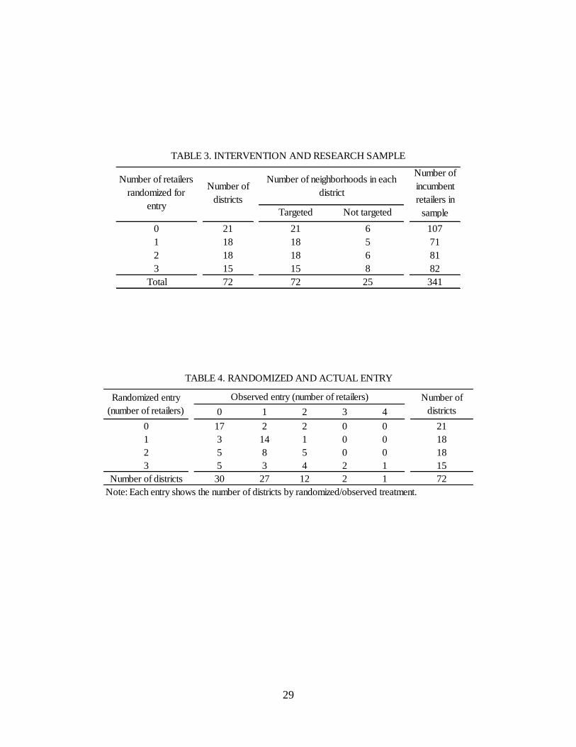
29

Targeted Not targeted

0 21 21 6 107

1 18 18 5 71

2 18 18 6 81

3 15 15 8 82

Total 72 72 25 341

Number of neighborhoods in each

district

Number of retailers

randomized for

entry

Number of

districts

Number of

incumbent

retailers in

sample

TABLE 3. INTERVENTION AND RESEARCH SAMPLE

0 1 2 3 4

0 17 2 2 0 0 21

1 3 14 1 0 0 18

2 5 8 5 0 0 18

3 5 3 4 2 1 15

Number of districts 30 27 12 2 1 72

Observed entry (number of retailers)Randomized entry

(number of retailers)

TABLE 4. RANDOMIZED AND ACTUAL ENTRY

Number of

districts

Note: Each entry shows the number of districts by randomized/observed treatment.

30

p-value of Number of

[1] [2] [3] [4]

Log (total beneficiaries - 2010) 6.441 6.453 0.960 72

[1.016] [0.865]

Change in log (total beneficiaries - 2009/2010) 0.211 0.172 0.380 72

[0.200] [0.160]

Log (sales - 2010) 11.149 11.340 0.573 69

[1.466] [1.165]

Change in log (sales -2009/2010) 1.033 1.231 0.803 67

[2.709] [2.991]

Number of incumbent retailers - 2010 6.714 5.745 0.577 72

[7.590] [6.273]

Change in log (number of retailers - 2009/2010) 0.442 0.444 0.987 72

[0.614] [0.647]

% Solidaridad program beneficiaries / population 0.325 0.383 0.151 72

[0.151] [0.244]

Average monthly household income (US$) 475.252 499.273 0.293 72

[91.933] [85.583]

% of population with completed primary education or lower0.628 0.613 0.444 72

[0.075] [0.078]

% of population with incomplete secondary education 0.213 0.208 0.735 72

[0.053] [0.051]

% of population with completed secondary education or higher0.159 0.179 0.207 72

[0.050] [0.064]

1 (if district is urban) 0.796 0.770 0.806 72

[0.400] [0.400]

District includes non-targeted neighborhoods 0.286 0.373 0.489 72

[0.463] [0.488]

Log-price index - pre-treatment (weighted) -0.323 -0.338 0.189 400

[0.080] [0.082]

Product-quality index 0.407 0.407 0.992 400

[0.052] [0.059]

Price range 0.329 0.281 0.277 361

[0.326] [0.307]

Product-quality range 1.501 1.509 0.316 361

[1.713] [1.559]

Brand-quality range 0.893 0.874 0.907 361

[0.949] [0.895]

Variety-quality range 1.048 1.183 0.973 361

[0.981] [0.970]

Percentage male 0.853 0.839 0.725 401

[0.356] [0.368]

1 (if the surveyed person is the retailer's owner) 0.688 0.623 0.119 401

[0.465] [0.485]

1 (if has more than a completed primary education) 0.679 0.613 0.197 401

[0.469] [0.488]

Log (total employees) 1.412 1.526 0.064 401

[0.440] [0.482]

Log (sales) 9.088 9.106 0.855 388

[0.767] [0.857]

Share of retailers in targeted neighborhood 0.615 0.651 0.781 401

[0.489] [0.478]

Log demeaned price (weighted) -3.588 -3.588 0.970 2125

[0.092] [0.092]

Service quality (rating 1-10) 8.979 8.983 0.975 2248

[1.600] [1.413]

Head of household's age 53.021 52.346 0.523 2250

[15.642] [15.257]

Monthly household income (US$) 475.369 498.549 0.315 2250

[265.401] [262.765]

% of heads of household who are married 0.576 0.538 0.293 2250

[0.495] [0.499]

% of head of household who work 0.557 0.532 0.311 2250

[0.497] [0.499]

% of head of household who are male 0.635 0.618 0.620 2250

[0.482] [0.486]

Note: Columns [1] and [2] report the mean and standar deviation (in square brackets) of each variable for the

neighborhoods with no (randomized) entry and with some (randomized) entry. Column [3] reports the p-value of a t-

test of the difference between the two samples (using clustered standard errors at the district level). Column [4] shows

the number of observations used.

Outcomes

Covariates

B. Retailer characteristics

Outcomes

Covariates

Other Variables

C. Consumer characteristics

Other variables

TABLE 5. DIFFERENCES IN PRE-TREATMENT SAMPLE MEANS

A. District characteristics

obs.

Control:

no entry

Treatment:

some entry difference

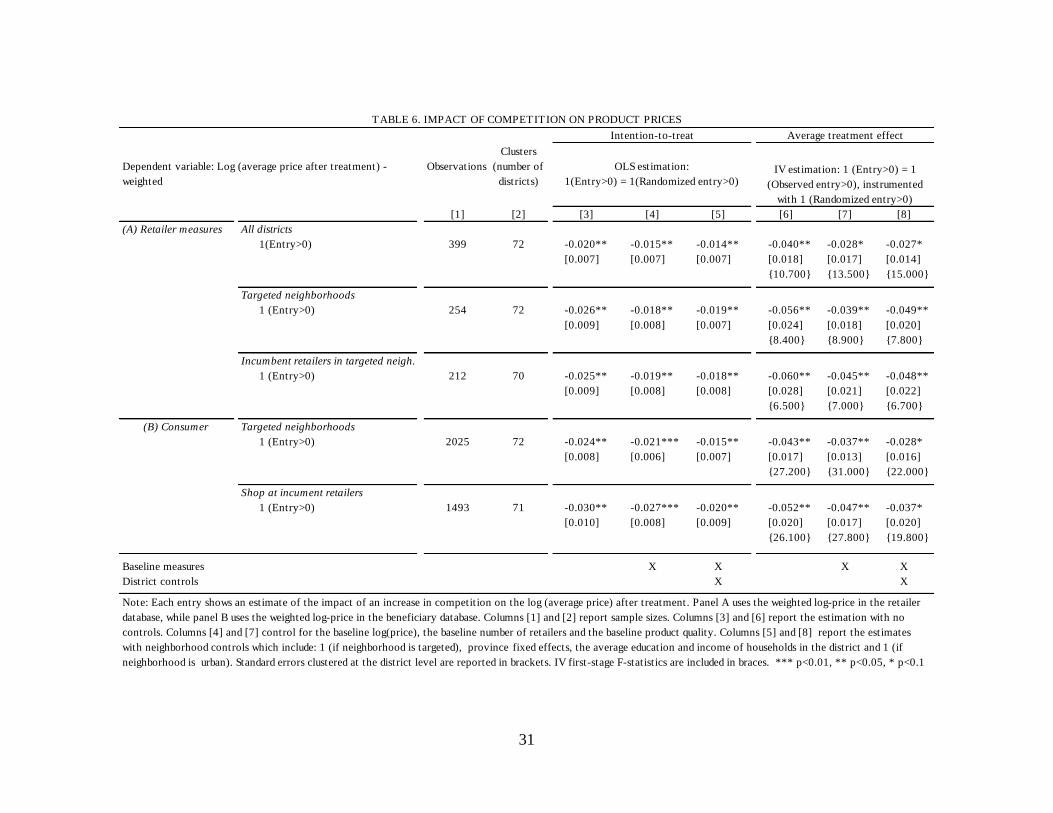
31

[1] [2] [3] [4] [5] [6] [7] [8]

(A) Retailer measures All districts

1(Entry>0) 399 72 -0.020** -0.015** -0.014** -0.040** -0.028* -0.027*

[0.007] [0.007] [0.007] [0.018] [0.017] [0.014]

{10.700} {13.500} {15.000}

Targeted neighborhoods

1 (Entry>0) 254 72 -0.026** -0.018** -0.019** -0.056** -0.039** -0.049**

[0.009] [0.008] [0.007] [0.024] [0.018] [0.020]

{8.400} {8.900} {7.800}

Incumbent retailers in targeted neigh.

1 (Entry>0) 212 70 -0.025** -0.019** -0.018** -0.060** -0.045** -0.048**

[0.009] [0.008] [0.008] [0.028] [0.021] [0.022]

{6.500} {7.000} {6.700}

(B) Consumer Targeted neighborhoods

1 (Entry>0) 2025 72 -0.024** -0.021*** -0.015** -0.043** -0.037** -0.028*

[0.008] [0.006] [0.007] [0.017] [0.013] [0.016]

{27.200} {31.000} {22.000}

Shop at incument retailers

1 (Entry>0) 1493 71 -0.030** -0.027*** -0.020** -0.052** -0.047** -0.037*

[0.010] [0.008] [0.009] [0.020] [0.017] [0.020]

{26.100} {27.800} {19.800}

Baseline measures X X X X

District controls X X

Note: Each entry shows an estimate of the impact of an increase in competition on the log (average price) after treatment. Panel A uses the weighted log-price in the retailer

database, while panel B uses the weighted log-price in the beneficiary database. Columns [1] and [2] report sample sizes. Columns [3] and [6] report the estimation with no

controls. Columns [4] and [7] control for the baseline log(price), the baseline number of retailers and the baseline product quality. Columns [5] and [8] report the estimates

with neighborhood controls which include: 1 (if neighborhood is targeted), province fixed effects, the average education and income of households in the district and 1 (if

neighborhood is urban). Standard errors clustered at the district level are reported in brackets. IV first-stage F-statistics are included in braces. *** p<0.01, ** p<0.05, * p<0.1

IV estimation: 1 (Entry>0) = 1

(Observed entry>0), instrumented

with 1 (Randomized entry>0)

Average treatment effect

TABLE 6. IMPACT OF COMPETITION ON PRODUCT PRICES

Observations

Clusters

(number of

districts)

Dependent variable: Log (average price after treatment) -

weighted

Intention-to-treat

OLS estimation:

1(Entry>0) = 1(Randomized entry>0)

32

[1] [2] [3] [4] [5] [6] [7] [8]

All neighborhoods

1(Randomized entry=1) 399 72 -0.020** -0.011 0.002 -0.034** -0.016 0.016

[0.009] [0.009] [0.009] [0.016] [0.016] [0.023]

1(Randomized entry=2 or 3) -0.020** -0.016** -0.019** -0.047 -0.037 -0.058*

[0.008] [0.008] [0.008] [0.029] [0.026] [0.033]

{17.200} {16.800} {7.900}

Targeted neighborhoods

1(Randomized entry=1) 254 72 -0.023** -0.014 -0.008 -0.034* -0.020 0.010

[0.011] [0.010] [0.010] [0.020] [0.019] [0.031]

1(Randomized entry=2 or 3) -0.027** -0.020** -0.025*** -0.071** -0.054* -0.087*

[0.010] [0.009] [0.008] [0.035] [0.029] [0.048]

{10.700} {10.800} {5.500}

Incumbent retailers in targeted neigh.

1(Randomized entry=1) 212 70 -0.028** -0.019* -0.013 -0.043** -0.028 -0.006

[0.011] [0.010] [0.010] [0.021] [0.021] [0.024]

1(Randomized entry=2 or 3) -0.023** -0.018** -0.021** -0.072* -0.058 -0.070*

[0.011] [0.009] [0.008] [0.041] [0.035] [0.039]

{9.100} {9.400} {5.100}

Baseline measures X X X X

District controls X X

TABLE 7. IMPACT OF ENTRY ON PRICES

(Heterogeneity)

Note: All entries report the estimation of a model in which the dependent variable is the log(average price) and the independent variables are dummies

indicating the level of treatment (D=1,2,3) and controls. Columns [1] and [2] report sample sizes. Columns [3] and [6] report the estimation with no

controls. Columns [4] and [7] control for the baseline log(average price), the baseline number of retailers and the baseline product quality. Columns [5]

and [8] report the estimates with neighborhood controls: 1 (if neighborhood is targeted), province fixed effects, the average education and income of

households in the district and 1(if neighborhood is urban). Standard errors clustered at the district level are reported in brackets. IV first-stage F-statistics

are included in braces. *** p<0.01, ** p<0.05, * p<0.1

Dependent variable:

Log(average price after treatment)

- weighted

Observation

s (number

of retailers)

Clusters

(number of

districts)

Intention-to-treat Average treatment effect

OLS estimation:

1(Entry=1) = 1(Randomized entry=1)

1(Entry=2,3,4) = 1(Randomized

entry=2,3)

IV estimation: 1(Entry=j)=1(Observed

entry=j), instrumented with 1(Randomized

entry=j), j=1,2 or more

33

[1] [2] [3] [4] [5]

(A) Retailer measures All districts

399 72 -0.033 -0.035 -0.062**

[0.026] [0.024] [0.027]

{36.100} {35.700} {36.300}

Targeted neighborhoods

254 72 -0.052** -0.053** -0.096***

[0.026] [0.024] [0.030]

{26.900} {28.000} {27.600}

Incumbent retailers in targeted neigh.

212 70 -0.077** -0.075** -0.105**

[0.038] [0.037] [0.040]

{19.500} {20.300} {17.700}

(B) Consumer measures Targeted neighborhoods

2025 72 -0.029* -0.024 -0.017

[0.016] [0.015] [0.016]

{56.600} {54.200} {74.900}

Shop at incument retailers

1493 71 -0.037** -0.031* -0.031

[0.018] [0.018] [0.021]

{36.200} {34.400} {54.500}

Baseline measures X X

Districts controls X

Note: Each entry shows an estimate of the impact of an increase in competition on the log weighted average price. Panel A

uses the weighted log-price in the retailer database, while panel B uses the weighted log-price in the consumer database.

Columns [1] and [2] report sample sizes. Column [3] reports the estimation with no controls. Column [4] controls for the

baseline log(price) and product-quality index. Columns [5] ] reports the estimates with district controls (province fixed effects

and total number of beneficiaries within the district at baseline). Standard errors clustered at the district level are reported in

brackets. IV first-stage F-statistics are included in braces. *** p<0.01, ** p<0.05, * p<0.1

TABLE 8. PRICE ELASTICITY OF ENTRY

IV estimatesDependent variable: Log (average price after treatment) -

weighted

Observation

s

Clusters

(number of

districts)

og 1 0

og 1 0

og 1 0

og 1 0

og 1 0

34

[1] [2] [3] [4] [5] [6] [7] [8]

(A) Retailer measures All districts

No CCT retailers 1(Entry>0) 63 33 -0.003 0.004 0.028 -0.006 0.007 0.065

[0.023] [0.019] [0.022] [0.041] [0.031] [0.059]

{10.100} {11.600} {3.300}

(B) Retailer measures No targeted neighborhoods

CCT retailers 1(Entry>0) 136 25 -0.014 -0.010 0.010 -0.024 -0.015 0.012

[0.013] [0.011] [0.033] [0.024] [0.019] [0.037]

{5.900} {9.500} {32.000}

Baseline measures X X X X

District controls X X

TABLE 9. IMPACT OF COMPETITION ON PRODUCT PRICES

Note: Each entry shows an estimate of the impact of an increase in competition on the log (average price) after treatment. Panel A uses the weighted log-price in

the retailer database, while panel B uses the weighted log-price in the beneficiary database. Columns [1] and [2] report sample sizes. Columns [3] and [6] report the

estimation with no controls. Columns [4] and [7] control for the baseline log(price), the baseline number of retailers and the baseline product quality. Columns [5]

and [8] report the estimates with neighborhood controls : 1 (if neighborhood is targeted), province fixed effects, the average education and income of households in

the district and 1(if neighborhood is urban). Standard errors clustered at the district level are reported in brackets. IV first-stage F-statistics are included in braces.

*** p<0.01, ** p<0.05, * p<0.1

(Non-CCT stores - No target areas)

Observations

(number of

retailers)

Clusters

(number of

districts)

Intention-to-treat Average treatment effect

Dependent variable: Log (average price after

treatment) -weighted

OLS estimation:

1(Entry>0) = 1(Randomized entry>0)

IV estimation: 1 (Entry>0) =

1(Observed entry>0), instrumented

with 1(Randomized entry>0)

35

Outcome: Log(Product quality index) -

weighted

[1] [2] [3] [4] [5] [6] [7] [8]

All districts 399 72 -0.006 -0.005 -0.002 -0.011 -0.01 -0.004

1(Entry>0) [0.007] [0.007] [0.006] [0.013] [0.013] [0.012]

{10.700} {13.500} {15.000}

Targeted neighborhoods 254 72 -0.013 -0.010 -0.008 -0.028 -0.021 -0.019

1 (Entry>0) [0.011] [0.011] [0.007] [0.020] [0.022] [0.017]

{8.400} {8.900} {7.800}

Incumbent retailers in targeted neigh. 212 70 -0.01 -0.007 -0.003 -0.024 -0.017 -0.009

1 (Entry>0) [0.011] [0.011] [0.008] [0.024] [0.025] [0.019]

{6.500} {7.000} {6.700}

Baseline measures X X X X

District controls X X

Note: Each entry shows an estimate of the impact of an increase in competition on quality after treatment. Panel A uses the

weighted log-price in the retailer database, while panel B uses the weighted log-price in the beneficiary database. Columns [1] and [2]

report sample sizes. Columns [3] and [6] report the estimation with no controls. Columns [4] and [7] control for the baseline

log(price), the baseline number of retailers and the baseline product quality. Columns [5] and [8] report the estimates with

neighborhood controls : 1(if neighborhood is targeted), province fixed effects, the average education and income of households in

the district and 1(if neighborhood is urban). Standard errors clustered at the district level are reported in brackets.IV first-stage F-

statistics are included in braces. *** p<0.01, ** p<0.05, * p<0.1

TABLE 10. IMPACT OF COMPETITION ON PRODUCT QUALITY

Observations Clusters

(number of

districts)

OLS estimation:

1 (Entry>0) = 1 (Randomized

entry>0)

Intention-to-treat IV estimation: 1 (Entry>0) =1

(Observed entry>0),

instrumented with 1

(Randomized entry>0)

Average treatment effect

36

Outcome

[1] [2] [3] [4] [5] [6] [7] [8]

Service quality (quality ladder)

Price range 235 72 -0.031 -0.019 0.008 -0.068 -0.042 0.021

[0.075] [0.068] [0.061] [0.170] [0.151] [0.152]

{8.400} {9.500} {8.000}

Product-quality range 235 72 0.597** 0.496* 0.236 1.324** 1.134* 0.632

[0.250] [0.276] [0.213] [0.606] [0.631] [0.561]

{8.400} {8.000} {6.900}

Quality range brand 235 72 0.337 0.187 0.006 0.748 0.427 0.016

[0.249] [0.271] [0.215] [0.485] [0.556] [0.546]

{8.400} {8.000} {6.800}

Variety-quality range 235 72 0.090 0.076 -0.034 0.201 0.177 -0.092

[0.109] [0.109] [0.104] [0.226] [0.235] [0.273]

{8.400} {7.800} {6.800}

Service quality

Number of brands offered in district 72 72 0.090 0.071 0.045 0.162 0.139 0.093

[0.249] [0.073] [0.087] [0.431] [0.126] [0.142]

{27.000} {21.000} {14.300}

Store cleanliness 254 72 0.105 0.142 0.142 0.228 0.309 0.372

[0.290] [0.266] [0.295] [0.614] [0.552] [0.721]

{8.400} {8.100} {7.300}

Log (employees) 254 72 0.067 -0.019 -0.038 0.145 -0.041 -0.095

[0.087] [0.056] [0.048] [0.168] [0.127] [0.127]

{8.400} {8.800} {7.700}

Time shopping (minutes) 2117 72 4.691 2.384 1.879 8.385 4.242 3.624

[4.531] [4.111] [3.984] [8.115] [7.311] [7.661]

{27.200} {30.500} {21.500}

Delivery 2118 72 0.056 0.044 0.040 0.100 0.078 0.076

[0.063] [0.044] [0.042] [0.111] [0.077] [0.079]

{27.200} {30.800} {21.900}

Service-quality rating 2116 72 0.213** 0.235*** 0.200** 0.380** 0.416** 0.379**

[0.090] [0.076] [0.069] [0.192] [0.168] [0.159]

{27.200} {30.900} {21.900}

Baseline measures X X X X

District controls X X

Note: Each entry shows an estimate of the impact of an increase in competition on quality after treatment. Panel A uses the

weighted log-price in the retailer database, while panel B uses the weighted log-price in the beneficiary database. Columns [1] and [2]

report sample sizes. Columns [3] and [6] report the estimation with no controls. Columns [4] and [7] control for the baseline

log(price), the baseline number of retailers, the baseline product quality, and the baseline value of the dependent variable. Columns

[5] and [8] report the estimates with neighborhood controls : 1 (if neighborhood is targeted), province fixed effects, the average

education and income of households in the district and 1 (if neighborhood is urban). Standard errors clustered at the district level are

reported in brackets.IV first-stage F-statistics are included in braces. *** p<0.01, ** p<0.05, * p<0.1

TABLE 11. IMPACT OF COMPETITION ON QUALITY

(Targeted districts)

Observations Clusters

(number of

districts)

Intention-to-treat Average treatment effect

OLS estimation:

1 (Entry>0) =

1 (Randomized entry>0)

IV estimation: 1 (Entry>0) =

1(Observed entry>0),

instrumented with

1(Randomized entry>0)

37

Outcome

[1] [2] [3] [4] [5] [6] [7] [8]

(A) Retailer measures

Number of customers on best day 254 72 -15.665 -9.667 -11.160 -33.898 -19.883 -27.090

[37.136] [37.985] [35.894] [84.195] [78.688] [85.438]

{8.400} {11.000} {8.700}

Share of customers CCT beneficiaries 228 70 -5.244 -4.613 -4.810* -12.211 -10.861 -13.432

[3.799] [3.096] [2.753] [9.907] [8.708] [10.069]

{8.400} {8.200} {6.300}

(B) Consumer measures

Switch to entrant retailer 1400 71 0.057*** 0.055*** 0.072** 0.099** 0.095** 0.146**

[0.018] [0.016] [0.024] [0.035] [0.032] [0.056]

{27.200} {31.000} {22.000}

Baseline measures X X X X

District controls X X

Note: Each entry shows an estimate of the impact of an increase in competition on several outcomes after treatment. Panel A uses information from the retailer

database, while panel B uses information from the beneficiary database. Columns [1] and [2] reports sample sizes. Columns [3] and [6] report the estimation with no

controls. Columns [4] and [7] control for the baseline log(price), the baseline number of retailers, the baseline product quality, and the baseline value of the dependent

variable. Columns [5] and [8] report the estimates with neighborhood controls : 1(if neighborhood is targeted), province fixed effects, the average education and

income of households in the district and 1(if neighborhood is urban). Standard errors clustered at the district level are reported in brackets. IV first-stage F-statistics are

included in braces. *** p<0.01, ** p<0.05, * p<0.1

TABLE 12. IMPACTS OF COMPETITION ON CLIENTELE

(Targeted districts)

Observations Clusters

(number of

districts)

Intention-to-treat Average treatment effect

OLS estimation:

1 (Entry>0) = 1 (Randomized entry>0)

IV estimation: 1 (Entry>0) =1

(Observed entry>0), instrumented with

1 (Randomized entry>0)

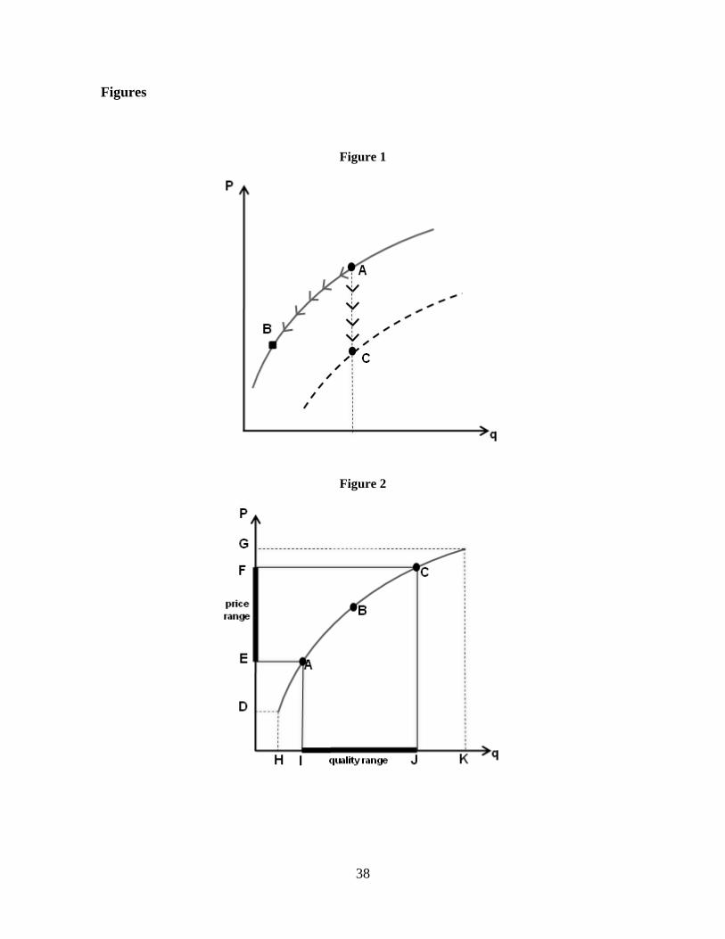
38

Figures

Figure 1

Figure 2

Online Appendix

- 1 -

Appendix I: Measures of Prices, Product Quality and Service Quality

1. Data Sources

Price and product-quality data are obtained from the responses to three questions (sources).

First, the retail survey questionnaire included a question (Question Q1) about 15 products.

Retailers were asked about the brand and price of the cheapest brand that is normally

available at their stores. This question pre-specified the unit of measurement. Second, in

Question Q2, retailers were asked to identify the three products that they sell the most of to

program beneficiaries and to provide information about the price, brand, variety and unit of

measurement for three different versions of these three products. Finally, in Question Q3,

consumers were asked about their weekly expenditure and the physical amount that they

bought of each of the 15 products in the last 7 days.

2. Coding Varieties and Brands

In order to code all possible combinations of brand-variety for each product, we pooled all

three sources of information. A unique code was assigned to each combination of brand-

variety for each of the 15 products. Q1 and Q3 were intended to only deal with brands. In

some instances, however, survey respondents mixed brands with varieties. For some

products, information about the variety could be recovered from the question even when the

respondent did not identify the variety, since in some cases the brand is associated with a

particular variety. This imputation of missing information was based on data obtained from

the webpages for each product.

Number

Varieties Brands

Rice 5 364

Cocking Oil 5 14

Sugar 2 30

Pasta 5 15

Eggs 3 42

Milk 5 29

Chocolate 2 4

Sardines 3 31

Beans 5 64

Onions 2 11

Salami 2 71

Chicken 2 32

Cod 3 7

Flour 3 34

Bread 0 102

Two issues warrant discussion. First, the variety of the products is often not associated with

a single characteristic. This is more frequently the case for some products than for others.

For instance, the variety of eggs could differ because of their size, yolk quality, etc. So in

Online Appendix

- 2 -

those cases, varieties were grouped together even though the relevant attributes differ.

Second, neither retailers nor consumers provided information about varieties of bread. The

previous table showed the complete list of brands and varieties for each product in our

sample.

3. Rankings

An average price was calculated for each brand/variety combination based on the

information provided in the retailers’ responses to Q1 and Q2 at baseline. Whenever the

information was not available at baseline, we used endline information from retailers in the

control areas. If there was any brand/variety combination for which no average price was

available, we calculated it using information obtained from retailers in treated areas.

Source Brand/Variety Brand Variety

N % N % N %

Baseline 833 0.654

509 0.648

58 0.951

Endline control areas 214 0.168

146 0.186

2 0.033

Endline treated areas 226 0.178 130 0.166 1 0.016

1273 785 61

Using these average prices, we calculated a percentile ranking of brand/varieties for each

one of the 15 products: (i) for each product, brand/variety combinations were ranked in

ascending order; (ii) this ranking was divided by the total number of possible combinations

of brand/varieties for each product. Call this measure 𝑣𝑖𝑡𝑘 for each product k, retailer i and

time t (t=baseline, endline). Therefore, the higher the average price, the higher the ranking.

We interpret this ranking as a measure of product quality.

4. Measures

We use this price and product-quality information to calculate price and quality indices for

retailers and consumers.

Average Price (retailers). For each retailer i at time t (t=baseline, endline), we computed

the average over all 15 products (k):

𝑃𝑖𝑡 = ∑𝑊𝑘 ∗ 𝑝𝑖𝑡𝑘

15

𝑘=1

In the case of the weighted average price, Wk is the share of expenditure on product k (see

below). In the case of the unweighted average price, Wk=1/15 for all k.

Online Appendix

- 3 -

Average Price (consumer). For each consumer i at time t (t=baseline, endline), we

computed the average (relative) price over all 15 products (k):

𝑃𝑖𝑡 = ∑𝑊𝑘 ∗ [𝑝𝑖𝑡𝑘𝑃𝑘𝑡̅̅ ̅̅

]

𝐾

𝑘=1

In the case of the weighted average price, Wk is the share of expenditure on product k (see

below). In the case of the unweighted average price, Wk=1/K for all k. Many consumers did

not report spending for all 15 products. To avoid differences in average prices due to

bundle composition, we standardized the price of each product using its average price in the

sample.

Quality Index (retailers). For each retailer i at time t (t=baseline, endline), we computed the

average over all 15 products (k):

𝑉𝑖𝑡 = ∑𝑊𝑘 ∗ 𝑣𝑖𝑡𝑘

𝐾

𝑘=1

In the case of the weighted quality index, Wk is the share of expenditure on product k (see

below). In the case of the unweighted quality index, Wk=1/15 for all k.

Number of Brands (district). In each district s at time t, we computed:

𝐵 𝑛𝑑 𝑠𝑡 = ∑𝑁𝑠𝑡𝑘

15

𝐾

𝑘=1

This is the average number of brands over the total number of products k that were

available in district s at time t according to the answers provided by retailers.

Price Range (retailers). Using Q2 for each retailer i at time t (t=baseline, endline), we

computed the average over three products for the price range:

∑ (𝑃𝑚 𝑥𝑘/𝑃𝑚 𝑛𝑘)3𝑘=1

3

where 𝑃𝑚 𝑥𝑘 = 𝑀 𝑥({𝑝 𝑐 𝑘𝑙}𝑙=13 ) and 𝑃𝑚 𝑛𝑘 = 𝑀 𝑛({𝑝 𝑐 𝑘𝑙}𝑙=1

3 ). This is the average

price range for the prices reported by the retailers for the three products (brands/varieties)

that they sell the most of to their customers. The price range is the ratio of the higher and

lower prices for each of these three products.

Quality Range (retailers). Using Q2 for each retailer i at time t (t=baseline, endline), we

computed the average over three products for the price range:

Online Appendix

- 4 -

∑ (𝑉𝑚 𝑥𝑘/𝑉𝑚 𝑛𝑘)3𝑘=1

3

where 𝑃𝑚 𝑥𝑘 = 𝑀 𝑥({𝑣𝑘𝑙}𝑙=13 ) and 𝑃𝑚 𝑛𝑘 = 𝑀 𝑛({𝑣𝑘𝑙}𝑙=1

3 ). This is the average quality

range for the qualities (brand/varieties) reported by the retailers for the three products

(brand/varieties) that they sell the most of to their customers. The quality range is the ratio

of the higher and lower quality for each of these three products. A version of this quality-

range measure was calculated using the ranking that was estimated using just the rankings

of the brands or the rankings of the varieties separately. We call these measures the

“Quality-range brand” and “Quality-range variety”.

5. Weights

The weights 𝑊𝑘 for the 15 products were created using the household survey. The weights

represent the share of monthly expenditure on product k made by all the surveyed

households at baseline. In all measures, the weights add up to 1.

The weights 𝑊𝑘 were compared with the results of a nationally representative survey of

program beneficiaries, the Evaluation Survey of Social Protection (EEPS), which was

conducted in 2010/2011. In this survey, households were queried about their expenditure on

a broader set of products. Appendix Table F1 indicates the results of this comparison. The

first column shows the product and the second column, the sample size. The third column

shows the percentage of households that reported having consumed a given product in the

previous week. The fourth column shows the average share of expenditure on each product.

Panel A gives the corresponding information for the 15 products that were covered in our

survey. Panel B summarizes the information about other non-perishable products that may

be sold by small-scale retailers. Panel C shows the measures for other fresh or perishable

products typically not sold by the retailers in question.

Several facts are worth mentioning here. First, the 15 products included in our survey

account for 60% of total food expenditure. Second, the other products that are sold by the

retailers under analysis represent 12% of total food expenditure. Third, most households

bought these 15 products. Fourth, the weights calculated in our sample are very close to

those observed in the EEPS.

Online Appendix

- 5 -

NPercentage

consumption

Share of

expenditure

Share of

expenditure

in price

index

Survey

weightings

Fifteen survey products 0.601 1.000 1.000

Rice 6783 0.962 0.157 0.262 0.293

Chicken 6784 0.784 0.089 0.148 0.170

Oil 6786 0.936 0.059 0.099 0.094

Milk 6786 0.338 0.045 0.075 0.062

Sugar 6785 0.955 0.045 0.075 0.052

Beans 6785 0.849 0.043 0.072 0.063

Salami 6786 0.758 0.039 0.064 0.048

Eggs 6785 0.792 0.030 0.051 0.050

Bread 6785 0.755 0.028 0.046 0.074

Pasta 6786 0.771 0.019 0.032 0.017

Onion 6785 0.886 0.018 0.030 0.020

Cod 6785 0.192 0.011 0.018 0.018

Sardines 6786 0.216 0.009 0.014 0.014

Chocolate 6784 0.366 0.007 0.011 0.015

Flour 6786 0.278 0.002 0.003 0.010

Other non-perishable products 0.121

Powdered chicken bouillon 6786 0.874 0.025 - -

Coffee 6785 0.708 0.023 - -

Water 6786 0.485 0.017 - -

Tomato paste 6786 0.715 0.017 - -

Soda 6786 0.296 0.012 - -

Smoked cutlets 6785 0.142 0.008 - -

Powdered juice 6786 0.287 0.007 - -

Ice 6786 0.329 0.005 - -

Pigeon peas 6785 0.123 0.004 - -

Dried coconut 6785 0.085 0.002 - -

Canned green beans 6785 0.026 0.001 - -

Fresh or persihable products 0.264

White cheese 6785 0.336 0.017 - -

Milk 6784 0.237 0.007 - -

Yellow cheese 6786 0.113 0.005 - -

Butter 6786 0.255 0.004 - -

Orange juice 6786 0.072 0.003 - -

Plantains 6785 0.723 0.037 - -

Avocados 6784 0.787 0.022 - -

Garlic 6785 0.900 0.022 - -

Beef 6785 0.240 0.020 - -

Pork 6785 0.232 0.019 - -

Yucca 6784 0.526 0.014 - -

Green bananas 6785 0.650 0.014 - -

Chili peppers 6782 0.749 0.009 - -

Fresh fish 6782 0.096 0.008 - -

Potatoes 6785 0.252 0.007 - -

Other vegetables 6784 0.604 0.006 - -

Eggplants 6785 0.303 0.005 - -

Squash 6785 0.399 0.005 - -

Peas 6786 0.134 0.005 - -

Clupea (fish) 6785 0.147 0.005 - -

Lemons 6783 0.401 0.004 - -

Tomatoes 6785 0.243 0.004 - -

Chayote 6785 0.237 0.003 - -

Cabbage 6784 0.194 0.003 - -

Bananas 6786 0.271 0.003 - -

Carrots 6786 0.175 0.003 - -

Sweet potatoes 6785 0.114 0.002 - -

Yautia 6785 0.073 0.002 - -

Other fruits 6786 0.095 0.002 - -

Beetroot 6785 0.064 0.001 - -

Oranges 6786 0.115 0.001 - -

Mangos 6786 0.055 0.001 - -

Product

EEPS 2010

APPENDIX TABLE F1: EEPS 2010/2011 - SHARE OF EXPENDINTURE ON ALL PRODUCTS

Note: The products in each of the three product groups are listed in descending order of share of

expenditure.

Online Appendix

- 6 -

6. Price Validation

In order to assess the validity of our price measures, we compare price measures obtained

using retailer data with those obtained using beneficiary data (an independent source of

information). For each product and brand in all the districts, we calculated an average price

based on the prices reported by the retailers and by the beneficiaries. Let �̅�𝑘𝑠𝑅 be the

average price in district s of product k computed using retailer information R, which

corresponds to the cheapest available option for each product. Similarly, let �̅�𝑘𝑠𝐶 be the

average price in district s computed using consumers’ information C which corresponds to

the products actually bought by consumers. The average district relative price (�̅�𝑘𝑠𝑅 /�̅�𝑘𝑠

𝐶 ) is

a useful statistic for assessing how close these two measures are. Note that, without

measurement error in the measures of prices, this statistic is bounded from above at 1. The

next figure shows a kernel density estimation of that price ratio. We find that the average

relative price over all products and districts is 0.99.

(�̅�𝑘𝑠𝑅 /�̅�𝑘𝑠

𝐶 ) Distribution

Mean: 0.9852S.D.: 0.2291

01

23

0 1 2 3Price Ratio Retailers/Consumers

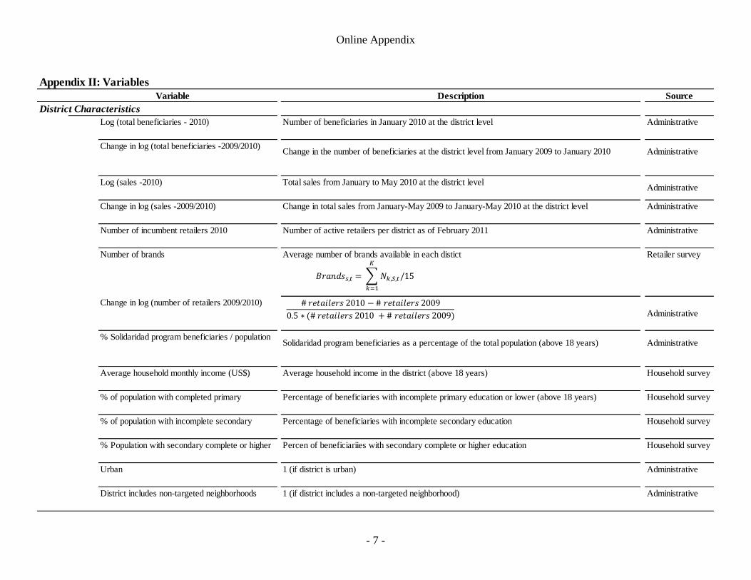
Online Appendix

- 7 -

Description Source

Log (total beneficiaries - 2010) Number of beneficiaries in January 2010 at the district level Administrative

Log (sales -2010) Total sales from January to May 2010 at the district level

Change in total sales from January-May 2009 to January-May 2010 at the district level Administrative

Number of incumbent retailers 2010 Number of active retailers per district as of February 2011 Administrative

Number of brands Average number of brands available in each distict Retailer survey

Change in log (number of retailers 2009/2010)

Administrative

% Solidaridad program beneficiaries / populationSolidaridad program beneficiaries as a percentage of the total population (above 18 years) Administrative

Average household monthly income (US$) Average household income in the district (above 18 years) Household survey

% of population with completed primary Percentage of beneficiaries with incomplete primary education or lower (above 18 years) Household survey

% of population with incomplete secondary Percentage of beneficiaries with incomplete secondary education Household survey

% Population with secondary complete or higher Percen of beneficiariies with secondary complete or higher education Household survey

Urban 1 (if district is urban) Administrative

District includes non-targeted neighborhoods 1 (if district includes a non-targeted neighborhood) Administrative

Appendix II: Variables

District Characteristics

Change in log (total beneficiaries -2009/2010)Change in the number of beneficiaries at the district level from January 2009 to January 2010 Administrative

Variable

Administrative

Change in log (sales -2009/2010)

𝐵 𝑛𝑑 𝑠,𝑡 = ∑ 𝑁𝑘,𝑆,𝑡/15

𝐾

𝑘=1

2010 − 200

0 5 ∗ ( 2010 + 200 )

Online Appendix

- 8 -

, where:

Price of product k in retailer i

Weight computed from the household survey

K is the number of products available at the store

Average Price (unweighted) Retailer survey

K is the number of products available at the store

, where:

Quality (ranking in prices) of product k in retailer i

Weight computed from the household survey

: Quality (ranking in prices) of product k in retailer i

Household and

retailer surveys

Quality is computed by ranking the different product brands based on their average price. Therefore,

a more expensive product is considered to be of better quality.

Producer quality index (unweighted)Retailer survey

Retailer Characteristics

Outcomes

Average Price (weighted)

Household and

retailer surveys

Product quality index (weighted)

Quality is computed by ranking the different product brands based on their average price. Therefore,

a more expensive product is considered to be of better quality.

𝑃𝑖𝑡 = ∑𝑊𝑘 ∗ 𝑝𝑖𝑡𝑘

𝐾

𝑘=1𝑝𝑖𝑘

𝑊𝑘

og(𝑃𝑖0)

𝑃𝑖𝑡 = ∑𝑊𝑘 ∗ 𝑝𝑖𝑡𝑘

𝐾

𝑘=1

𝑊𝑘 = 𝑘

∑ 𝑘𝐾𝑘=1

𝑊𝑘 =1

𝑉𝑖𝑡 = ∑𝑊𝑘 ∗ 𝑣𝑖𝑡𝑘

𝐾

𝑘=1

𝑣𝑖𝑡𝑘𝑊𝑘

𝑊𝑘 = 𝑘

∑ 𝑘𝐾𝑘=1

𝑉𝑖𝑡 = ∑ 𝑣𝑖𝑡𝑘

𝐾𝑘=1

𝑞𝑖𝑡𝑘

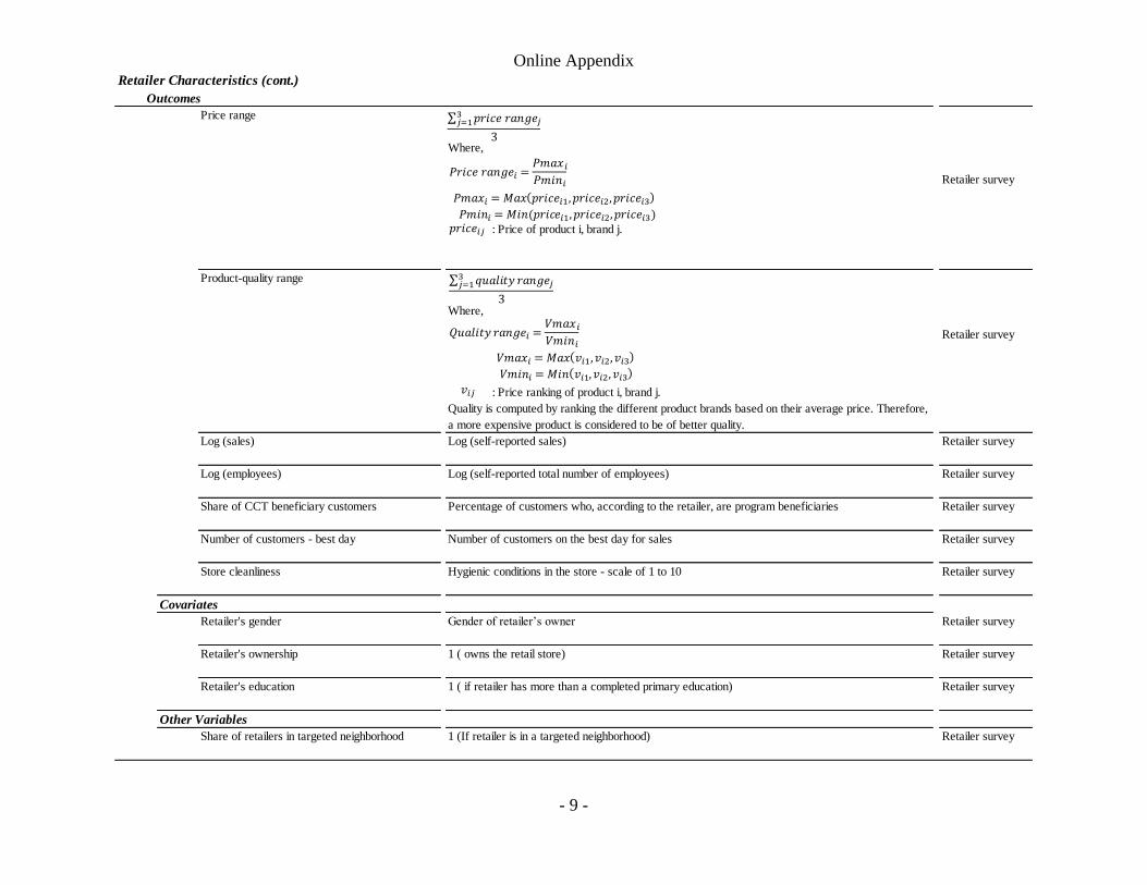
Online Appendix

- 9 -

Where,

: Price of product i, brand j.

Where,

: Price ranking of product i, brand j.

Log (sales) Log (self-reported sales) Retailer survey

Log (employees) Log (self-reported total number of employees) Retailer survey

Share of CCT beneficiary customers Percentage of customers who, according to the retailer, are program beneficiaries Retailer survey

Number of customers - best day Number of customers on the best day for sales Retailer survey

Store cleanliness Hygienic conditions in the store - scale of 1 to 10 Retailer survey

Covariates

Retailer's gender Gender of retailer’s owner Retailer survey

Retailer's ownership 1 ( owns the retail store) Retailer survey

Retailer's education 1 ( if retailer has more than a completed primary education) Retailer survey

Other Variables

Share of retailers in targeted neighborhood 1 (If retailer is in a targeted neighborhood) Retailer survey

Retailer Characteristics (cont.)

Retailer survey

Product-quality range

Retailer survey

Quality is computed by ranking the different product brands based on their average price. Therefore,

a more expensive product is considered to be of better quality.

Outcomes

Price range ∑ 𝑝 𝑐 𝑛 𝑗3𝑗=1

3

𝑃 𝑐 𝑛 𝑖 =𝑃𝑚 𝑥𝑖𝑃𝑚 𝑛𝑖

𝑃𝑚 𝑥𝑖 = 𝑀 𝑥 𝑝 𝑐 𝑖1, 𝑝 𝑐 𝑖2, 𝑝 𝑐 𝑖3𝑃𝑚 𝑛𝑖 = 𝑀 𝑛(𝑝 𝑐 𝑖1, 𝑝 𝑐 𝑖2, 𝑝 𝑐 𝑖3)

𝑝 𝑐 𝑖𝑗

∑ 𝑞 𝑛 𝑗3𝑗=1

3

𝑛 𝑖 =𝑉𝑚 𝑥𝑖𝑉𝑚 𝑛𝑖

𝑉𝑚 𝑥𝑖 = 𝑀 𝑥 𝑣𝑖1, 𝑣𝑖2, 𝑣𝑖3𝑉𝑚 𝑛𝑖 = 𝑀 𝑛 𝑣𝑖1, 𝑣𝑖2, 𝑣𝑖3

𝑣𝑖𝑗

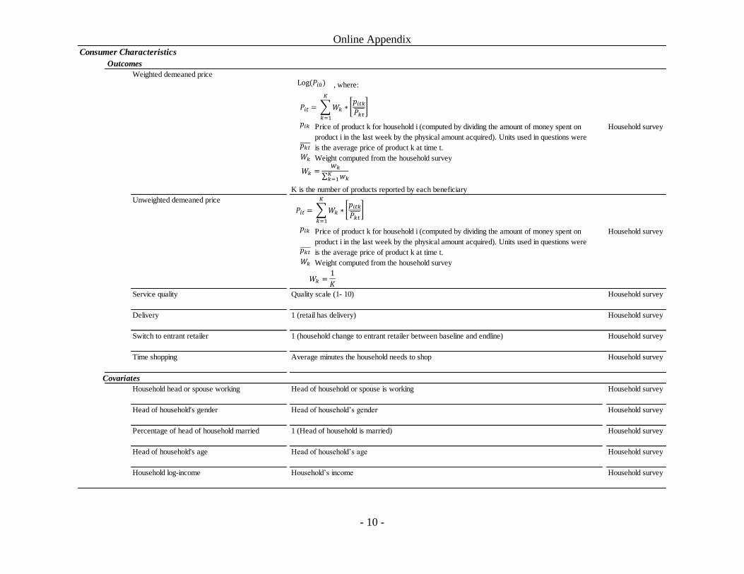
Online Appendix

- 10 -

Weighted demeaned price

, where:

Household survey

is the average price of product k at time t.

Weight computed from the household survey

K is the number of products reported by each beneficiary

Unweighted demeaned price

Household survey

is the average price of product k at time t.

Weight computed from the household survey

Service quality Quality scale (1- 10) Household survey

Delivery 1 (retail has delivery) Household survey

Switch to entrant retailer 1 (household change to entrant retailer between baseline and endline) Household survey

Time shopping Average minutes the household needs to shop Household survey

Household head or spouse working Head of household or spouse is working Household survey

Head of household's gender Head of household’s gender Household survey

Percentage of head of household married 1 (Head of household is married) Household survey

Head of household's age Head of household’s age Household survey

Household log-income Household’s income Household survey

Covariates

Outcomes

Price of product k for household i (computed by dividing the amount of money spent on

product i in the last week by the physical amount acquired). Units used in questions were

Price of product k for household i (computed by dividing the amount of money spent on

product i in the last week by the physical amount acquired). Units used in questions were

Consumer Characteristics

𝑃𝑖𝑡 = ∑𝑊𝑘 ∗𝑝𝑖𝑡𝑘𝑃𝑘𝑡

𝐾

𝑘=1

𝑊𝑘 = 𝑘

∑ 𝑘𝐾𝑘=1

𝑊𝑘 =1

og(𝑃𝑖0)

𝑝𝑖𝑘

𝑝𝑘𝑡

𝑊𝑘

𝑃𝑖𝑡 = ∑𝑊𝑘 ∗𝑝𝑖𝑡𝑘𝑃𝑘𝑡

𝐾

𝑘=1

𝑝𝑖𝑘

𝑝𝑘𝑡

𝑊𝑘

Online Appendix

- 11 -

Appendix III: Robustness and Extensions

At At

baseline endline

Universe of retailers in area under study 432 425

Universe of entrant retailers 61 61

Sample size: Retailers (in surveys) 401 400

By type

Incumbent 350 341

Entrant 51 59

Located in targeted neighborhood 257 254

Incumbent in targeted neighborhood 215 212

Sample size: Beneficiaries (in surveys) 2250 2118

By type

Shop in incumbent retailers 1620 1563

Located in targeted neighborhood 2250 2118

Number of districts 72 72

TABLE A1. SAMPLE SIZE

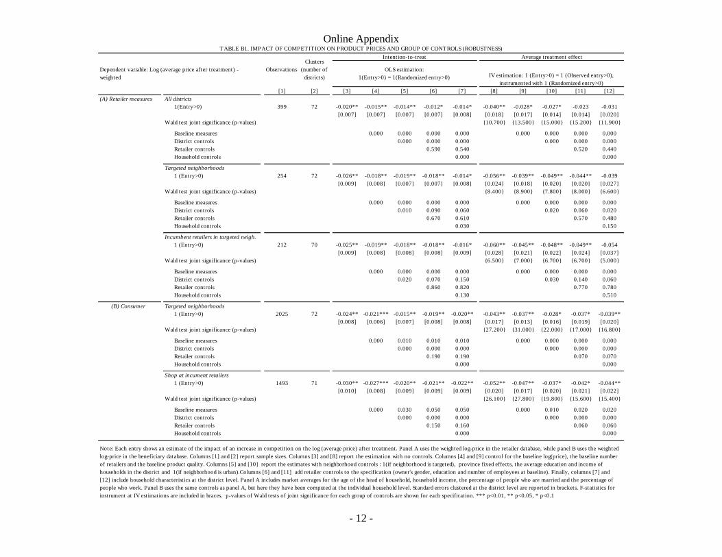
Online Appendix

- 12 -

[1] [2] [3] [4] [5] [6] [7] [8] [9] [10] [11] [12]

(A) Retailer measures All districts

1(Entry>0) 399 72 -0.020** -0.015** -0.014** -0.012* -0.014* -0.040** -0.028* -0.027* -0.023 -0.031

[0.007] [0.007] [0.007] [0.007] [0.008] [0.018] [0.017] [0.014] [0.014] [0.020]

Wald test joint significance (p-values) {10.700} {13.500} {15.000} {15.200} {11.900}

Baseline measures 0.000 0.000 0.000 0.000 0.000 0.000 0.000 0.000

District controls 0.000 0.000 0.000 0.000 0.000 0.000

Retailer controls 0.590 0.540 0.520 0.440

Household controls 0.000 0.000

Targeted neighborhoods

1 (Entry>0) 254 72 -0.026** -0.018** -0.019** -0.018** -0.014* -0.056** -0.039** -0.049** -0.044** -0.039

[0.009] [0.008] [0.007] [0.007] [0.008] [0.024] [0.018] [0.020] [0.020] [0.027]

Wald test joint significance (p-values) {8.400} {8.900} {7.800} {8.000} {6.600}

Baseline measures 0.000 0.000 0.000 0.000 0.000 0.000 0.000 0.000

District controls 0.010 0.090 0.060 0.020 0.060 0.020

Retailer controls 0.670 0.610 0.570 0.480

Household controls 0.030 0.150

Incumbent retailers in targeted neigh.

1 (Entry>0) 212 70 -0.025** -0.019** -0.018** -0.018** -0.016* -0.060** -0.045** -0.048** -0.049** -0.054

[0.009] [0.008] [0.008] [0.008] [0.009] [0.028] [0.021] [0.022] [0.024] [0.037]

Wald test joint significance (p-values) {6.500} {7.000} {6.700} {6.700} {5.000}

Baseline measures 0.000 0.000 0.000 0.000 0.000 0.000 0.000 0.000

District controls 0.020 0.070 0.150 0.030 0.140 0.060

Retailer controls 0.860 0.820 0.770 0.780

Household controls 0.130 0.510

(B) Consumer Targeted neighborhoods

1 (Entry>0) 2025 72 -0.024** -0.021*** -0.015** -0.019** -0.020** -0.043** -0.037** -0.028* -0.037* -0.039**

[0.008] [0.006] [0.007] [0.008] [0.008] [0.017] [0.013] [0.016] [0.019] [0.020]

Wald test joint significance (p-values) {27.200} {31.000} {22.000} {17.000} {16.800}

Baseline measures 0.000 0.010 0.010 0.010 0.000 0.000 0.000 0.000

District controls 0.000 0.000 0.000 0.000 0.000 0.000

Retailer controls 0.190 0.190 0.070 0.070

Household controls 0.000 0.000

Shop at incument retailers

1 (Entry>0) 1493 71 -0.030** -0.027*** -0.020** -0.021** -0.022** -0.052** -0.047** -0.037* -0.042* -0.044**

[0.010] [0.008] [0.009] [0.009] [0.009] [0.020] [0.017] [0.020] [0.021] [0.022]

Wald test joint significance (p-values) {26.100} {27.800} {19.800} {15.600} {15.400}

Baseline measures 0.000 0.030 0.050 0.050 0.000 0.010 0.020 0.020

District controls 0.000 0.000 0.000 0.000 0.000 0.000

Retailer controls 0.150 0.160 0.060 0.060

Household controls 0.000 0.000

Note: Each entry shows an estimate of the impact of an increase in competition on the log (average price) after treatment. Panel A uses the weighted log-price in the retailer database, while panel B uses the weighted

log-price in the beneficiary database. Columns [1] and [2] report sample sizes. Columns [3] and [8] report the estimation with no controls. Columns [4] and [9] control for the baseline log(price), the baseline number

of retailers and the baseline product quality. Columns [5] and [10] report the estimates with neighborhood controls : 1(if neighborhood is targeted), province fixed effects, the average education and income of

households in the district and 1(if neighborhood is urban).Columns [6] and [11] add retailer controls to the specification (owner's gender, education and number of employees at baseline). Finally, columns [7] and

[12] include household characteristics at the district level. Panel A includes market averages for the age of the head of household, household income, the percentage of people who are married and the percentage of

people who work. Panel B uses the same controls as panel A, but here they have been computed at the individual household level. Standard errors clustered at the district level are reported in brackets. F-statistics for

instrument at IV estimations are included in braces. p-values of Wald tests of joint significance for each group of controls are shown for each specification. *** p<0.01, ** p<0.05, * p<0.1

TABLE B1. IMPACT OF COMPETITION ON PRODUCT PRICES AND GROUP OF CONTROLS (ROBUSTNESS)

Observations

Clusters

(number of

districts)

Intention-to-treat Average treatment effect

Dependent variable: Log (average price after treatment) -

weighted

OLS estimation:

1(Entry>0) = 1(Randomized entry>0) IV estimation: 1 (Entry>0) = 1 (Observed entry>0),

instrumented with 1 (Randomized entry>0)

Online Appendix

- 13 -

[1] [2] [3] [4] [5] [6] [7] [8]

(A) Retailer measures All districts

1(Entry>0) 399 72 -0.012 -0.012* -0.012 -0.023 -0.022 -0.024

[0.008] [0.007] [0.008] [0.019] [0.016] [0.016]

{10.700} {13.600} {14.900}

Targeted neighborhoods

1 (Entry>0) 254 72 -0.029** -0.026** -0.024** -0.063* -0.054* -0.062**

[0.010] [0.009] [0.008] [0.034] [0.028] [0.029]

{8.400} {8.800} {7.600}

Incumbent retailers in targeted neigh.

1 (Entry>0) 212 70 -0.027** -0.025** -0.022** -0.066* -0.058* -0.060*

[0.010] [0.010] [0.009] [0.039] [0.032] [0.031]

{6.500} {6.800} {6.400}

(B) Consumer measures

Targeted neighborhoods

1 (Entry>0) 2025 72 -0.024** -0.020** -0.015** -0.042** -0.035** -0.029*

[0.008] [0.007] [0.007] [0.016] [0.014] [0.016]

{27.200} {31.000} {22.000}

Shop at incument retailers

1 (Entry>0) 1493 71 -0.028*** -0.024** -0.018** -0.049** -0.042** -0.033*

[0.009] [0.008] [0.008] [0.020] [0.017] [0.019]

{26.100} {27.700} {19.700}

Baseline measures X X X X

District controls X X

Note: Each entry shows an estimate of the impact of an increase in competition on the log (price) after treatment. Panel A uses the unweighted log-price in the retailer

database, while panel B uses the unweighted log-price in the beneficiary database. Columns [1] and [2] report sample sizes. Columns [3] and [6] report the estimation with no

controls. Columns [4] and [7] control for the baseline log(price), the baseline number of retailers and the baseline product quality. Columns [5] and [8] report the estimates

with neighborhood controls : 1 (if neighborhood is targeted), province fixed effects, the average education and income of households in the district and 1 (if neighborhood is

urban). Standard errors clustered at the district level are reported in brackets. F-statistics for instrument at IV estimations are included in braces. p-values of Wald tests of joint

significance for each group of controls are shown for each specification. *** p<0.01, ** p<0.05, * p<0.1

TABLE B2. IMPACT OF COMPETITION ON UNWEIGHTED PRODUCT PRICES (ROBUSTNESS)

Observations

Clusters

(number of

districts)

Intention-to-treat Average treatment effect

Dependent variable: Log (average price after treatment) -

unweighted

OLS estimation:

1(Entry>0) = 1(Randomized entry>0)

IV estimation: 1 (Entry>0) = 1

(Observed entry>0), instrumented

with 1 (Randomized entry>0)

Online Appendix

- 14 -

[1] [2] [3] [4] [5] [6] [7] [8]

(A) Retailer measures All districts

1(Entry>0) 5645 72 -0.003 -0.005 -0.013 -0.005 -0.010 -0.025

[0.012] [0.010] [0.009] [0.023] [0.018] [0.017]

{10.600} {13.600} {15.600}

Targeted neighborhoods

1 (Entry>0) 3585 72 -0.025** -0.020* -0.020** -0.054* -0.042* -0.051*

[0.012] [0.012] [0.009] [0.032] [0.024] [0.029]

{8.400} {8.900} {8.100}

Incumbent retailers in targeted neigh.

1 (Entry>0) 2985 70 -0.020 -0.018 -0.018** -0.048 -0.043 -0.048

[0.013] [0.012] [0.009] [0.035] [0.027] [0.029]

{6.500} {6.900} {6.900}

(B) Consumer measures Targeted neighborhoods

1 (Entry>0) 16531 72 -0.026** -0.018** -0.015** -0.046** -0.031** -0.029*

[0.009] [0.009] [0.007] [0.018] [0.016] [0.015]

{27.200} {31.300} {21.700}

Shop at incument retailers

1 (Entry>0) 12102 71 -0.029** -0.022** -0.019** -0.052** -0.039** -0.036**

[0.010] [0.009] [0.007] [0.021] [0.018] [0.017]

{26.100} {25.300} {18.900}

Baseline measures X X X X

District controls X X

Note: Each entry shows an estimate of the impact of an increase in competition on the log (price) after treatment. Panel A uses the weighted log-price in the retailer database,

while panel B uses the weighted log-price in the beneficiary database. Columns [1] and [2] report sample sizes. Columns [3] and [6] report the estimation with no controls.

Columns [4] and [7] control for the baseline log(price), the baseline number of retailers and the baseline product quality. Columns [5] and [8] report the estimates with

neighborhood controls : 1 (if neighborhood is targeted), province fixed effects, the average education and income of households in the district and 1 (if neighborhood is

urban). Standard errors clustered at the district level are reported in brackets. F-statistics for instrument at IV estimations are included in braces. p-values of Wald tests of joint

significance for each group of controls are shown for each specification. *** p<0.01, ** p<0.05, * p<0.1

TABLE B3. IMPACT ON POOLED PRICES (ROBUSTNESS)

Observations

Clusters

(number of

districts)

Intention-to-treat Average treatment effect

Dependent variable: Log (average price after treatment) OLS estimation:

1(Entry>0) = 1(Randomized entry>0)

IV estimation: 1 (Entry>0) = 1

(Observed entry>0), instrumented

with 1 (Randomized entry>0)

Online Appendix

- 15 -

Weighting

Outcome Log(Product Price) ITT IV ITT IV ITT IV

[1] [2] [3] [4] [5] [6] [7]

Rice (lb.) 0.293 -0.008 -0.015 -0.010 -0.022 -0.009 -0.022

[0.013] [0.023] [0.017] [0.033] [0.018] [0.037]

Cooking oil (lb.) 0.094 -0.030** -0.057 -0.050*** -0.110** -0.052*** -0.129**

[0.015] [0.038] [0.015] [0.046] [0.016] [0.059]

Sugar (lb.) 0.052 -0.001 -0.002 -0.003 -0.007 -0.008 -0.019

[0.011] [0.020] [0.009] [0.020] [0.010] [0.023]

Pasta (lb.) 0.017 -0.027** -0.051** -0.048*** -0.102** -0.048** -0.113*

[0.013] [0.024] [0.015] [0.047] [0.016] [0.058]

Eggs (unit) 0.050 -0.022 -0.042 -0.025 -0.055 -0.025 -0.059

[0.026] [0.044] [0.023] [0.046] [0.022] [0.052]

Powdered milk (125 gr.) 0.062 0.032 0.060 0.019 0.040 0.006 0.015

[0.023] [0.042] [0.025] [0.054] [0.022] [0.053]

Chocolate (unit) 0.015 0.002 0.004 -0.008 -0.017 -0.009 -0.022

[0.011] [0.021] [0.014] [0.028] [0.014] [0.030]

Sardines (unit) 0.014 0.028 0.053 0.015 0.032 0.017 0.040

[0.032] [0.062] [0.044] [0.097] [0.042] [0.100]

Green beans (lb.) 0.063 -0.005 -0.009 -0.005 -0.011 -0.003 -0.007

[0.006] [0.011] [0.008] [0.017] [0.008] [0.020]

Onions (lb.) 0.020 -0.013 -0.024 -0.047** -0.104* -0.038* -0.092

[0.022] [0.044] [0.022] [0.062] [0.022] [0.066]

Salami (lb.) 0.048 -0.051* -0.096* -0.060 -0.132 -0.046 -0.111

[0.028] [0.054] [0.039] [0.091] [0.040] [0.099]

Chicken (lb.) 0.170 -0.014 -0.023 -0.008 -0.016 -0.008 -0.016

[0.009] [0.017] [0.014] [0.025] [0.014] [0.028]

Cod (lb.) 0.018 -0.010 -0.019 -0.020** -0.045 -0.023** -0.057

[0.009] [0.016] [0.010] [0.031] [0.010] [0.039]

Flour (lb.) 0.010 -0.038** -0.066** -0.042** -0.086* -0.040* -0.092

[0.015] [0.031] [0.020] [0.051] [0.021] [0.060]

Bread (unit) 0.074 0.088* 0.151 0.021 0.039 0.035 0.073

[0.052] [0.107] [0.057] [0.107] [0.057] [0.121]

TABLE B4: IMPACT ON INDIVIDUAL PRODUCT PRICES (ROBUSTNESS)

All Targeted Incumbents

Note: Each entry shows an estimate of the impact of an increase in competition on the price of different products. Column [1]

shows the weighting of each product in the final retailer price. Columns [2]-[3] use all the retailers ; columns [4]-[5] use retailers

in targeted neighborhoods; and columns [6]-[7] use incumbent retailers in targeted neigborhoods. All columns report the

estimations while controlling for the baseline log(price). *** p<0.01, ** p<0.05, * p<0.1

Online Appendix

- 16 -

[1] [2] [3] [4] [5] [4] [5]

(A) Retailer measures All districts

399 72 -0.033 -0.035 -0.062** -0.061** -0.068**

[0.026] [0.024] [0.027] [0.026] [0.030]

Wald test joint significance (p-values) {36.100} {35.700} {36.300} {36.200} {27.300}

Baseline measures 0.000 0.000 0.000 0.000

District controls 0.000 0.000 0.000

Retailer controls 0.510 0.430

Household controls 0.000

Targeted neighborhoods

254 72 -0.052** -0.053** -0.096*** -0.094*** -0.097**

[0.026] [0.024] [0.030] [0.030] [0.035]

Wald test joint significance (p-values) {26.900} {28.000} {27.600} {27.300} {21.900}

Baseline measures 0.000 0.000 0.000 0.000

District controls 0.010 0.020 0.240

Retailer controls 0.680 0.570

Household controls 0.240

Incumbent retailers in target neigh.

212 70 -0.077** -0.075** -0.105** -0.105** -0.115**

[0.038] [0.037] [0.040] [0.040] [0.049]

Wald test joint significance (p-values) {19.500} {20.300} {17.700} {17.200} {14.200}

Baseline measures 0.000 0.000 0.000 0.000

District controls 0.000 0.000 0.000

Retailer controls 0.830 0.830

Household controls 0.400

(B) Consumer measures Targeted neighborhoods

2025 72 -0.029* -0.024 -0.017 -0.030* -0.032*

[0.016] [0.015] [0.016] [0.017] [0.017]

Wald test joint significance (p-values) {56.600} {54.200} {74.900} {66.600} {66.300}

Baseline measures 0.000 0.010 0.040 0.040

District controls 0.000 0.000 0.000

Retailer controls 0.120 0.130

Household controls 0.000

Shop at Incument Retailers

1493 71 -0.037** -0.031* -0.031 -0.032 -0.035*

[0.018] [0.018] [0.021] [0.020] [0.020]

Wald test joint significance (p-values) {36.200} {34.400} {54.500} {52.900} {52.500}

Baseline measures 0.020 0.070 0.140 0.150

District controls 0.000 0.000 0.000

Retailer controls 0.090 0.100

Household controls 0.000

Note: Each entry shows an estimate of the impact of an increase in competition on the log average price weighted . Panel A uses the weighted log-price in the

retailer database, while panel B uses the weighted log-price in the beneficiary database. Columns [1] and [2] report sample sizes. Column [3] reports the

estimation with no controls. Column [4] controls for the baseline log(price) and product-quality index. Column [5] reports the estimates with neighborhood

controls : 1 (if neighborhood is targeted), province fixed effects, the average education and income of households in the district and 1 (if neighborhood is

urban).Column [6] adds retailer controls to the specification (owner's gender, education and number of employees at baseline). Finally, column [7] includes

household characteristics at the district level. Standard errors clustered at the district level are reported in brackets. F-statistics for instrument at IV estimations

are included in braces. p-values of Wald tests of joint significance for each group of controls are shown for each specification. *** p<0.01, ** p<0.05, * p<0.1

TABLE B5. PRICE ELASTICITY OF ENTRY GROUP OF CONTROLS

Dependent variable: Log (Average price after treatment) -

weighted

Observations Clusters (number

of districts)IV estimates

og 1 0

og 1 0

og 1 0

og 1 0

og 1 0

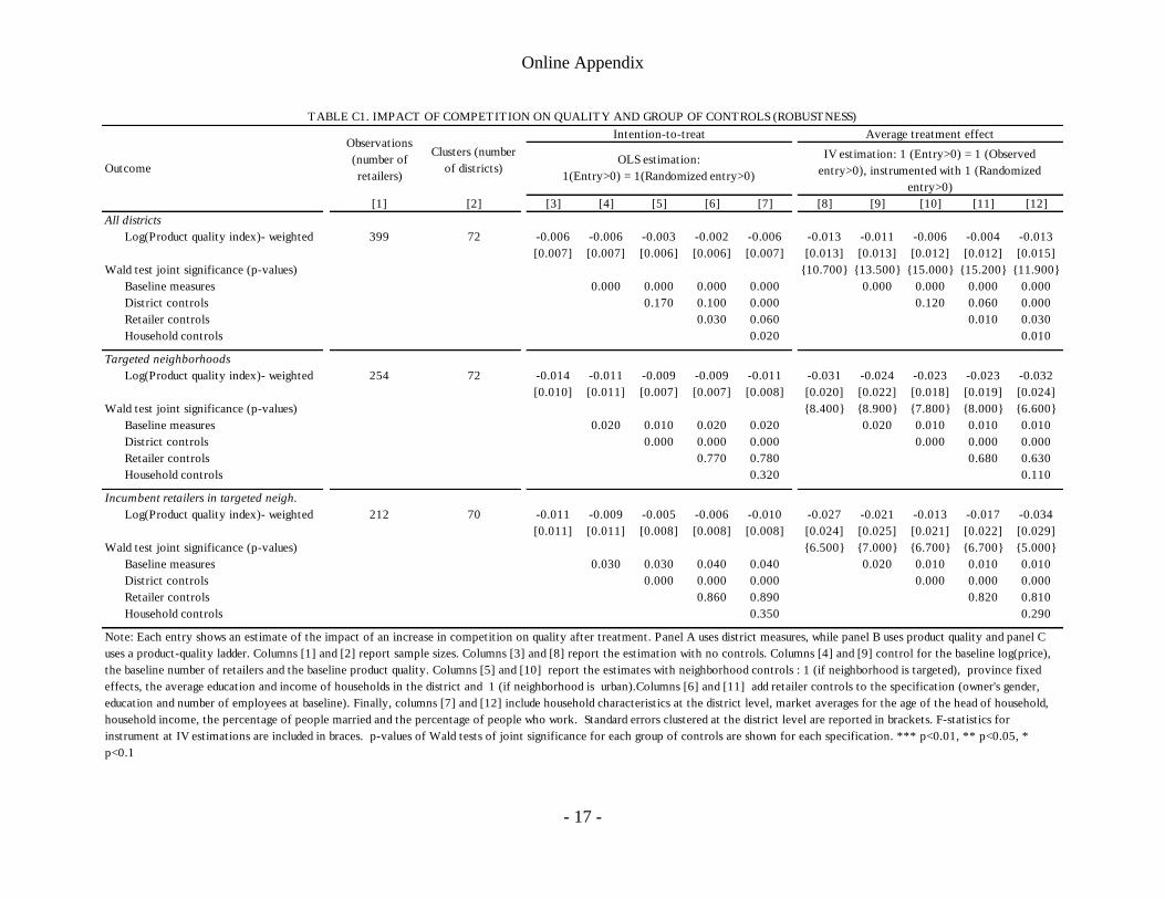
Online Appendix

- 17 -

Outcome

[1] [2] [3] [4] [5] [6] [7] [8] [9] [10] [11] [12]

All districts

Log(Product quality index)- weighted 399 72 -0.006 -0.006 -0.003 -0.002 -0.006 -0.013 -0.011 -0.006 -0.004 -0.013

[0.007] [0.007] [0.006] [0.006] [0.007] [0.013] [0.013] [0.012] [0.012] [0.015]

Wald test joint significance (p-values) {10.700} {13.500} {15.000} {15.200} {11.900}

Baseline measures 0.000 0.000 0.000 0.000 0.000 0.000 0.000 0.000

District controls 0.170 0.100 0.000 0.120 0.060 0.000

Retailer controls 0.030 0.060 0.010 0.030

Household controls 0.020 0.010

Targeted neighborhoods

Log(Product quality index)- weighted 254 72 -0.014 -0.011 -0.009 -0.009 -0.011 -0.031 -0.024 -0.023 -0.023 -0.032

[0.010] [0.011] [0.007] [0.007] [0.008] [0.020] [0.022] [0.018] [0.019] [0.024]

Wald test joint significance (p-values) {8.400} {8.900} {7.800} {8.000} {6.600}

Baseline measures 0.020 0.010 0.020 0.020 0.020 0.010 0.010 0.010

District controls 0.000 0.000 0.000 0.000 0.000 0.000

Retailer controls 0.770 0.780 0.680 0.630

Household controls 0.320 0.110

Incumbent retailers in targeted neigh.

Log(Product quality index)- weighted 212 70 -0.011 -0.009 -0.005 -0.006 -0.010 -0.027 -0.021 -0.013 -0.017 -0.034

[0.011] [0.011] [0.008] [0.008] [0.008] [0.024] [0.025] [0.021] [0.022] [0.029]

Wald test joint significance (p-values) {6.500} {7.000} {6.700} {6.700} {5.000}

Baseline measures 0.030 0.030 0.040 0.040 0.020 0.010 0.010 0.010

District controls 0.000 0.000 0.000 0.000 0.000 0.000

Retailer controls 0.860 0.890 0.820 0.810

Household controls 0.350 0.290

Note: Each entry shows an estimate of the impact of an increase in competition on quality after treatment. Panel A uses district measures, while panel B uses product quality and panel C

uses a product-quality ladder. Columns [1] and [2] report sample sizes. Columns [3] and [8] report the estimation with no controls. Columns [4] and [9] control for the baseline log(price),

the baseline number of retailers and the baseline product quality. Columns [5] and [10] report the estimates with neighborhood controls : 1 (if neighborhood is targeted), province fixed

effects, the average education and income of households in the district and 1 (if neighborhood is urban).Columns [6] and [11] add retailer controls to the specification (owner's gender,

education and number of employees at baseline). Finally, columns [7] and [12] include household characteristics at the district level, market averages for the age of the head of household,

household income, the percentage of people married and the percentage of people who work. Standard errors clustered at the district level are reported in brackets. F-statistics for

instrument at IV estimations are included in braces. p-values of Wald tests of joint significance for each group of controls are shown for each specification. *** p<0.01, ** p<0.05, *

p<0.1

TABLE C1. IMPACT OF COMPETITION ON QUALITY AND GROUP OF CONTROLS (ROBUSTNESS)

Observations

(number of

retailers)

Clusters (number

of districts)

Intention-to-treat Average treatment effect

OLS estimation:

1(Entry>0) = 1(Randomized entry>0)

IV estimation: 1 (Entry>0) = 1 (Observed

entry>0), instrumented with 1 (Randomized

entry>0)

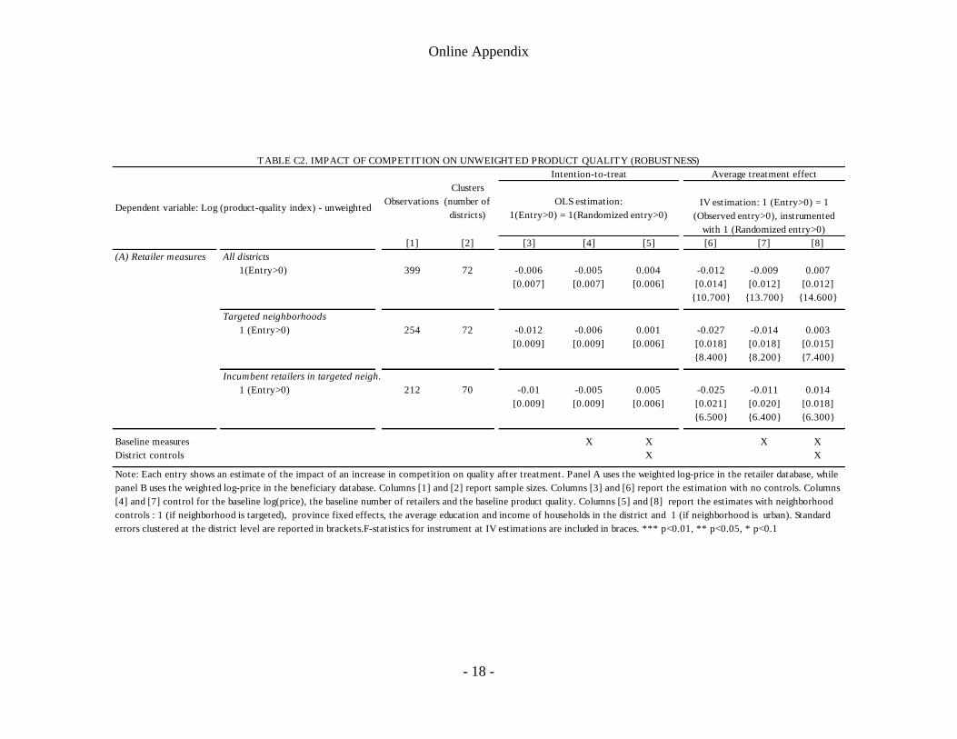
Online Appendix

- 18 -

[1] [2] [3] [4] [5] [6] [7] [8]

(A) Retailer measures All districts

1(Entry>0) 399 72 -0.006 -0.005 0.004 -0.012 -0.009 0.007

[0.007] [0.007] [0.006] [0.014] [0.012] [0.012]

{10.700} {13.700} {14.600}

Targeted neighborhoods

1 (Entry>0) 254 72 -0.012 -0.006 0.001 -0.027 -0.014 0.003

[0.009] [0.009] [0.006] [0.018] [0.018] [0.015]

{8.400} {8.200} {7.400}

Incumbent retailers in targeted neigh.

1 (Entry>0) 212 70 -0.01 -0.005 0.005 -0.025 -0.011 0.014

[0.009] [0.009] [0.006] [0.021] [0.020] [0.018]

{6.500} {6.400} {6.300}

Baseline measures X X X X

District controls X X

Note: Each entry shows an estimate of the impact of an increase in competition on quality after treatment. Panel A uses the weighted log-price in the retailer database, while

panel B uses the weighted log-price in the beneficiary database. Columns [1] and [2] report sample sizes. Columns [3] and [6] report the estimation with no controls. Columns

[4] and [7] control for the baseline log(price), the baseline number of retailers and the baseline product quality. Columns [5] and [8] report the estimates with neighborhood

controls : 1 (if neighborhood is targeted), province fixed effects, the average education and income of households in the district and 1 (if neighborhood is urban). Standard

errors clustered at the district level are reported in brackets.F-statistics for instrument at IV estimations are included in braces. *** p<0.01, ** p<0.05, * p<0.1

TABLE C2. IMPACT OF COMPETITION ON UNWEIGHTED PRODUCT QUALITY (ROBUSTNESS)

Observations

Clusters

(number of

districts)

Intention-to-treat Average treatment effect

Dependent variable: Log (product-quality index) - unweightedOLS estimation:

1(Entry>0) = 1(Randomized entry>0)

IV estimation: 1 (Entry>0) = 1

(Observed entry>0), instrumented

with 1 (Randomized entry>0)

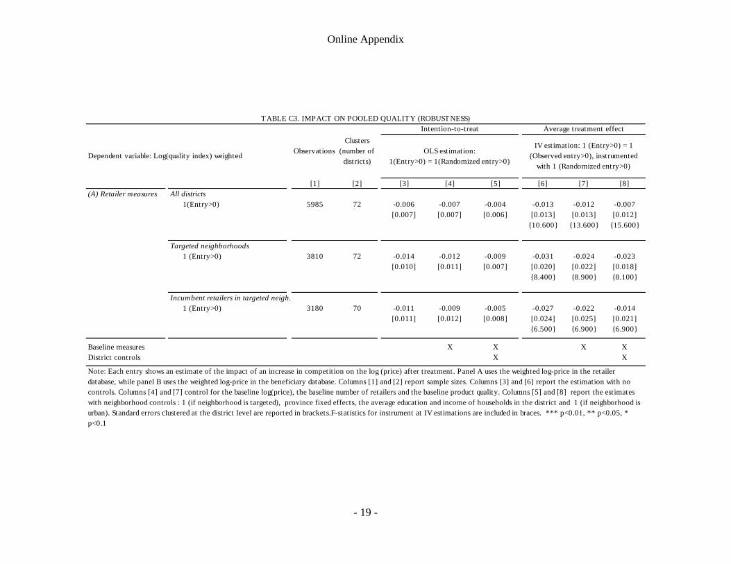
Online Appendix

- 19 -

[1] [2] [3] [4] [5] [6] [7] [8]

(A) Retailer measures All districts

1(Entry>0) 5985 72 -0.006 -0.007 -0.004 -0.013 -0.012 -0.007

[0.007] [0.007] [0.006] [0.013] [0.013] [0.012]

{10.600} {13.600} {15.600}

Targeted neighborhoods

1 (Entry>0) 3810 72 -0.014 -0.012 -0.009 -0.031 -0.024 -0.023

[0.010] [0.011] [0.007] [0.020] [0.022] [0.018]

{8.400} {8.900} {8.100}

Incumbent retailers in targeted neigh.

1 (Entry>0) 3180 70 -0.011 -0.009 -0.005 -0.027 -0.022 -0.014

[0.011] [0.012] [0.008] [0.024] [0.025] [0.021]

{6.500} {6.900} {6.900}

Baseline measures X X X X

District controls X X

Note: Each entry shows an estimate of the impact of an increase in competition on the log (price) after treatment. Panel A uses the weighted log-price in the retailer

database, while panel B uses the weighted log-price in the beneficiary database. Columns [1] and [2] report sample sizes. Columns [3] and [6] report the estimation with no

controls. Columns [4] and [7] control for the baseline log(price), the baseline number of retailers and the baseline product quality. Columns [5] and [8] report the estimates

with neighborhood controls : 1 (if neighborhood is targeted), province fixed effects, the average education and income of households in the district and 1 (if neighborhood is

urban). Standard errors clustered at the district level are reported in brackets.F-statistics for instrument at IV estimations are included in braces. *** p<0.01, ** p<0.05, *

p<0.1

TABLE C3. IMPACT ON POOLED QUALITY (ROBUSTNESS)

Observations

Clusters

(number of

districts)

Intention-to-treat Average treatment effect

Dependent variable: Log(quality index) weightedOLS estimation:

1(Entry>0) = 1(Randomized entry>0)

IV estimation: 1 (Entry>0) = 1

(Observed entry>0), instrumented

with 1 (Randomized entry>0)

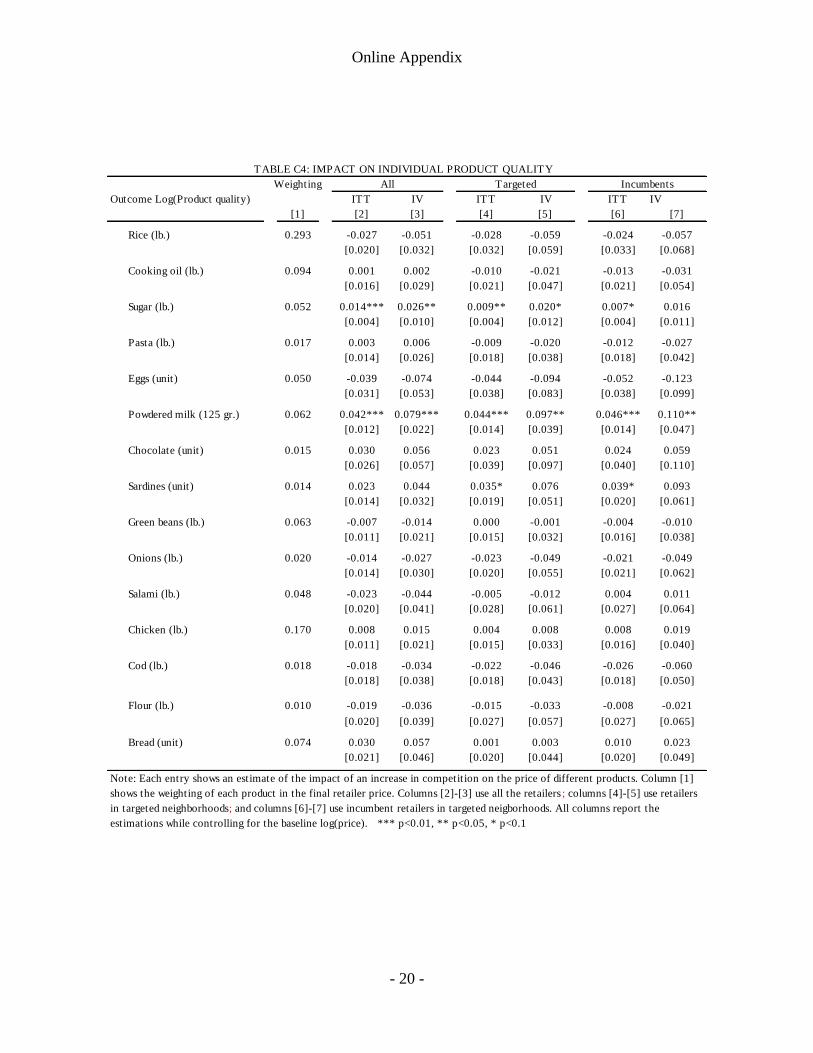
Online Appendix

- 20 -

Weighting

Outcome Log(Product quality) ITT IV ITT IV ITT IV

[1] [2] [3] [4] [5] [6] [7]

Rice (lb.) 0.293 -0.027 -0.051 -0.028 -0.059 -0.024 -0.057

[0.020] [0.032] [0.032] [0.059] [0.033] [0.068]

Cooking oil (lb.) 0.094 0.001 0.002 -0.010 -0.021 -0.013 -0.031

[0.016] [0.029] [0.021] [0.047] [0.021] [0.054]

Sugar (lb.) 0.052 0.014*** 0.026** 0.009** 0.020* 0.007* 0.016

[0.004] [0.010] [0.004] [0.012] [0.004] [0.011]

Pasta (lb.) 0.017 0.003 0.006 -0.009 -0.020 -0.012 -0.027

[0.014] [0.026] [0.018] [0.038] [0.018] [0.042]

Eggs (unit) 0.050 -0.039 -0.074 -0.044 -0.094 -0.052 -0.123

[0.031] [0.053] [0.038] [0.083] [0.038] [0.099]

Powdered milk (125 gr.) 0.062 0.042*** 0.079*** 0.044*** 0.097** 0.046*** 0.110**

[0.012] [0.022] [0.014] [0.039] [0.014] [0.047]

Chocolate (unit) 0.015 0.030 0.056 0.023 0.051 0.024 0.059

[0.026] [0.057] [0.039] [0.097] [0.040] [0.110]

Sardines (unit) 0.014 0.023 0.044 0.035* 0.076 0.039* 0.093

[0.014] [0.032] [0.019] [0.051] [0.020] [0.061]

Green beans (lb.) 0.063 -0.007 -0.014 0.000 -0.001 -0.004 -0.010

[0.011] [0.021] [0.015] [0.032] [0.016] [0.038]

Onions (lb.) 0.020 -0.014 -0.027 -0.023 -0.049 -0.021 -0.049

[0.014] [0.030] [0.020] [0.055] [0.021] [0.062]

Salami (lb.) 0.048 -0.023 -0.044 -0.005 -0.012 0.004 0.011

[0.020] [0.041] [0.028] [0.061] [0.027] [0.064]

Chicken (lb.) 0.170 0.008 0.015 0.004 0.008 0.008 0.019

[0.011] [0.021] [0.015] [0.033] [0.016] [0.040]

Cod (lb.) 0.018 -0.018 -0.034 -0.022 -0.046 -0.026 -0.060

[0.018] [0.038] [0.018] [0.043] [0.018] [0.050]

Flour (lb.) 0.010 -0.019 -0.036 -0.015 -0.033 -0.008 -0.021

[0.020] [0.039] [0.027] [0.057] [0.027] [0.065]

Bread (unit) 0.074 0.030 0.057 0.001 0.003 0.010 0.023

[0.021] [0.046] [0.020] [0.044] [0.020] [0.049]

TABLE C4: IMPACT ON INDIVIDUAL PRODUCT QUALITY

All Targeted Incumbents

Note: Each entry shows an estimate of the impact of an increase in competition on the price of different products. Column [1]

shows the weighting of each product in the final retailer price. Columns [2]-[3] use all the retailers ; columns [4]-[5] use retailers

in targeted neighborhoods; and columns [6]-[7] use incumbent retailers in targeted neigborhoods. All columns report the

estimations while controlling for the baseline log(price). *** p<0.01, ** p<0.05, * p<0.1

Online Appendix

- 21 -

Outcome

[1] [2] [3] [4] [5] [6] [7] [8]

Service quality (quality ladder)

Number of brands 72 72 0.090 0.071 0.045 0.162 0.139 0.093

[0.249] [0.073] [0.087] [0.431] [0.126] [0.142]

{27.000} {21.000} {14.300}

Price range 376 72 -0.048 -0.040 0.012 -0.097 -0.076 0.023

[0.055] [0.054] [0.047] [0.125] [0.106] [0.090]

{10.700} {14.000} {15.500}

Quality range 376 72 0.083 0.163 0.241 0.168 0.313 0.494

[0.257] [0.226] [0.213] [0.492] [0.432] [0.409]

{10.700} {12.200} {13.400}

Brand-quality range 376 72 0.139 0.158 0.075 0.280 0.303 0.153

[0.196] [0.175] [0.187] [0.346] [0.321] [0.354]

{10.700} {12.400} {13.200}

Variety-quality range 376 72 0.065 0.040 -0.046 0.130 0.077 -0.094

[0.078] [0.082] [0.088] [0.168] [0.160] [0.183]

{10.700} {12.200} {13.200}

Service quality

Store cleanliness 400 72 -0.037 -0.133 0.151 -0.074 -0.251 0.305

[0.213] [0.192] [0.229] [0.425] [0.376] [0.434]

{10.700} {12.700} {14.100}

Log (employees) 400 72 0.125* 0.044 -0.006 0.248** 0.082 -0.011

[0.065] [0.044] [0.044] [0.107] [0.075] [0.086]

{10.700} {13.200} {14.800}

Time shopping (minutes) 2117 72 4.691 2.384 1.879 8.385 4.242 3.624

[4.531] [4.111] [3.984] [8.115] [7.311] [7.661]

{27.200} {30.500} {21.500}

Delivery 2118 72 0.056 0.044 0.040 0.100 0.078 0.076

[0.063] [0.044] [0.042] [0.111] [0.077] [0.079]

{27.200} {30.800} {21.900}

Service-quality rating 2116 72 0.213** 0.235*** 0.200** 0.380** 0.416** 0.379**

[0.090] [0.076] [0.069] [0.192] [0.168] [0.159]

{27.200} {30.900} {21.900}

Baseline measures X X X X

District controls X X

Note: Each entry shows an estimate of the impact of an increase in competition on quality after treatment. Panel A uses the

weighted log-price in the retailer database, while panel B uses the weighted log-price in the beneficiary database. Columns [1]

and [2] report sample sizes. Columns [3] and [6] report the estimation with no controls. Columns [4] and [7] control for the

baseline log(price), the baseline number of retailers and the baseline product quality. Columns [5] and [8] report the estimates

with neighborhood controls : 1 (if neighborhood is targeted), province fixed effects, the average education and income of

households in the district and 1 (if neighborhood is urban). Standard errors clustered at the district level are reported in

brackets. F-statistics for instrument at IV estimations are included in braces. *** p<0.01, ** p<0.05, * p<0.1

TABLE D1. IMPACT OF COMPETITION ON QUALITY

(All districts)

Observations Clusters

(number of

districts)

Intention-to-treat Average treatment effect

OLS estimation:

1 (Entry>0) = 1 (Randomized

entry>0)

IV estimation: 1 (Entry>0) =1

(Observed entry>0),

instrumented with 1

(Randomized entry>0)

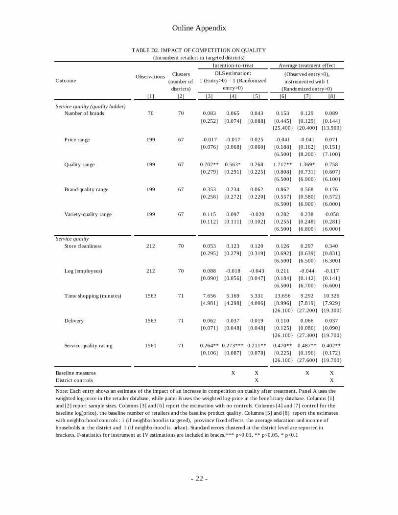
Online Appendix

- 22 -

Outcome

[1] [2] [3] [4] [5] [6] [7] [8]

Service quality (quality ladder)

Number of brands 70 70 0.083 0.065 0.043 0.153 0.129 0.089

[0.252] [0.074] [0.088] [0.445] [0.129] [0.144]

{25.400} {20.400} {13.900}

Price range 199 67 -0.017 -0.017 0.025 -0.041 -0.041 0.071

[0.076] [0.068] [0.060] [0.188] [0.162] [0.151]

{6.500} {8.200} {7.100}

Quality range 199 67 0.702** 0.563* 0.268 1.717** 1.369* 0.758

[0.279] [0.291] [0.225] [0.808] [0.731] [0.607]

{6.500} {6.900} {6.100}

Brand-quality range 199 67 0.353 0.234 0.062 0.862 0.568 0.176

[0.258] [0.272] [0.220] [0.557] [0.580] [0.572]

{6.500} {6.900} {6.000}

Variety-quality range 199 67 0.115 0.097 -0.020 0.282 0.238 -0.058

[0.112] [0.111] [0.102] [0.255] [0.248] [0.281]

{6.500} {6.800} {6.000}

Service quality

Store cleanliness 212 70 0.053 0.123 0.120 0.126 0.297 0.340

[0.295] [0.279] [0.319] [0.692] [0.639] [0.831]

{6.500} {6.500} {6.300}

Log (employees) 212 70 0.088 -0.018 -0.043 0.211 -0.044 -0.117

[0.090] [0.056] [0.047] [0.184] [0.142] [0.141]

{6.500} {6.700} {6.600}

Time shopping (minutes) 1563 71 7.656 5.169 5.331 13.656 9.292 10.326

[4.981] [4.298] [4.006] [8.996] [7.819] [7.929]

{26.100} {27.200} {19.300}

Delivery 1563 71 0.062 0.037 0.019 0.110 0.066 0.037

[0.071] [0.048] [0.048] [0.125] [0.086] [0.090]

{26.100} {27.300} {19.700}

Service-quality rating 1561 71 0.264** 0.273*** 0.211** 0.470** 0.487** 0.402**

[0.106] [0.087] [0.078] [0.225] [0.196] [0.172]

{26.100} {27.600} {19.700}

Baseline measures X X X X

District controls X X

Note: Each entry shows an estimate of the impact of an increase in competition on quality after treatment. Panel A uses the

weighted log-price in the retailer database, while panel B uses the weighted log-price in the beneficiary database. Columns [1]

and [2] report sample sizes. Columns [3] and [6] report the estimation with no controls. Columns [4] and [7] control for the

baseline log(price), the baseline number of retailers and the baseline product quality. Columns [5] and [8] report the estimates

with neighborhood controls : 1 (if neighborhood is targeted), province fixed effects, the average education and income of

households in the district and 1 (if neighborhood is urban). Standard errors clustered at the district level are reported in

brackets. F-statistics for instrument at IV estimations are included in braces.*** p<0.01, ** p<0.05, * p<0.1

TABLE D2. IMPACT OF COMPETITION ON QUALITY

(Incumbent retailers in targeted districts)

Observations Clusters

(number of

districts)

Intention-to-treat Average treatment effect

OLS estimation:

1 (Entry>0) = 1 (Randomized

entry>0)

IV estimation: 1 (Entry>0) =1

(Observed entry>0),

instrumented with 1

(Randomized entry>0)

Online Appendix

- 23 -

Outcome

[1] [2] [3] [4] [5] [6] [7] [8]

(A) Retailer measures

Number of customers on best day 400 72 -31.156 -39.497 -15.33 -61.893 -71.822 -29.384

[39.666] [39.963] [30.937] [77.982] [72.597] [59.618]

{10.700} {15.200} {16.800}

Share of customers CCT beneficiaries 366 70 0.464 -0.487 -1.258 0.946 -0.957 -2.682

[3.619] [3.437] [2.964] [7.189] [6.775] [6.233]

{10.700} {12.100} {12.200}

(B) Consumer measures

Switch to entrant retailer 1400 71 0.057*** 0.055*** 0.072** 0.099** 0.095** 0.146**

[0.018] [0.016] [0.024] [0.035] [0.032] [0.056]

{27.200} {31.000} {22.000}

Baseline measures X X X X

District controls X X

Note: Each entry shows an estimate of the impact of an increase in competition on several outcomes after treatment. Panel A uses information from the retailer

database, while panel B uses information from the beneficiary database. Columns [1] and [2] reports sample sizes. Columns [3] and [6] report the estimation with no

controls. Columns [4] and [7] control for the baseline log(price), the baseline number of retailers, the baseline product quality, and the baseline value of the dependent

variable. Columns [5] and [8] report the estimates with neighborhood controls : 1(if neighborhood is targeted), province fixed effects, the average education and

income of households in the district and 1(if neighborhood is urban). Standard errors clustered at the district level are reported in brackets. IV first-stage F-statistics are

included in braces. *** p<0.01, ** p<0.05, * p<0.1

TABLE E1. IMPACTS OF COMPETITION ON CLIENTELE

(All districts)

Observations Clusters

(number of

districts)

Intention-to-treat Average treatment effect

OLS estimation:

1 (Entry>0) = 1 (Randomized entry>0)

IV estimation: 1 (Entry>0) =1

(Observed entry>0), instrumented with

1 (Randomized entry>0)

Online Appendix

- 24 -

Outcome

[1] [2] [3] [4] [5] [6] [7] [8]

(A) Retailer measures

Number of customers on best day 212 70 -25 -17.025 -20.666 -59.866 -38.511 -53.615

[38.883] [38.453] [36.308] [101.946] [89.762] [96.822]

{6.500} {8.800} {7.500}

Share of customers CCT beneficiaries 193 64 -5.325 -4.732 -4.081 -13.763 -12.012 -12.027

[3.793] [3.096] [2.695] [11.338] [9.779] [9.856]

{6.500} {6.900} {5.600}

Baseline measures X X X X

District controls X X

Note: Each entry shows an estimate of the impact of an increase in competition on several outcomes after treatment. Panel A uses information from the retailer

database, while panel B uses information from the beneficiary database. Columns [1] and [2] reports sample sizes. Columns [3] and [6] report the estimation with no

controls. Columns [4] and [7] control for the baseline log(price), the baseline number of retailers, the baseline product quality, and the baseline value of the dependent

variable. Columns [5] and [8] report the estimates with neighborhood controls : 1(if neighborhood is targeted), province fixed effects, the average education and

income of households in the district and 1(if neighborhood is urban). Standard errors clustered at the district level are reported in brackets. IV first-stage F-statistics are

included in braces. *** p<0.01, ** p<0.05, * p<0.1

TABLE E2. IMPACT OF COMPETITION ON CLIENTELE

(Incumbent retailers in targeted districts)

Observations Clusters

(number of

districts)

Intention-to-treat Average treatment effect

OLS estimation:

1 (Entry>0) = 1 (Randomized entry>0)

IV estimation: 1 (Entry>0) =1

(Observed entry>0), instrumented with

1 (Randomized entry>0)