The Bregman Methods: Review and New Results - …optimization/L1/bregman/WotaoYin_Bregman... · The Bregman Methods: Review and New Results ... 0 50 100 150 200 250-2-1.5-1-0.5 0

The Bregman Methods: Review and New Results

Wotao Yin

Department of Computational and Applied Mathematics, Rice University

(Work supported by NSF, ONR, and Sloan Foundation)

December 8, 2009

Acknowledgements: results come in part from discussions with StanOsher, Christ Brune, and Martin Burger.

Bregman iteration has been unreasonably successful in

1. Improving the solution quality of regularizers such as `1, totalvariation, ...

2. Giving fast, accurate methods for constrained `1-like minimization.

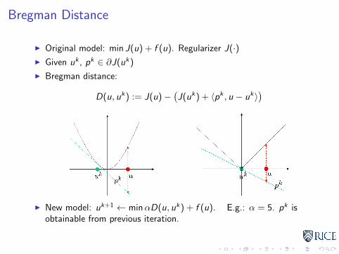
Bregman Distance

I Original model: min J(u) + f (u). Regularizer J(·)I Given uk , pk ∈ ∂J(uk)

I Bregman distance:

D(u, uk) := J(u)−(J(uk) + 〈pk , u − uk〉

)

I New model: uk+1 ← minαD(u, uk) + f (u). E.g.: α = 5. pk isobtainable from previous iteration.

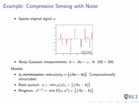
Example: Compressive Sensing with Noise

I Sparse original signal u

0 50 100 150 200 250−2

−1.5

−1

−0.5

0

0.5

1

1.5

2

true signal

I Noisy Gaussian measurements: b ← Au + ω. A: 100× 250.

Models:

I `0 minimization: minµ‖u‖0 + 12‖Au − b‖22. Computationally

intractable!

I Basis pursuit: u ← minµ‖u‖1 + 12‖Au − b‖22

I Bregman: uk+1 ← minD(u, uk) + 12‖Au − b‖22

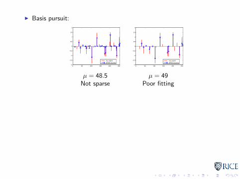
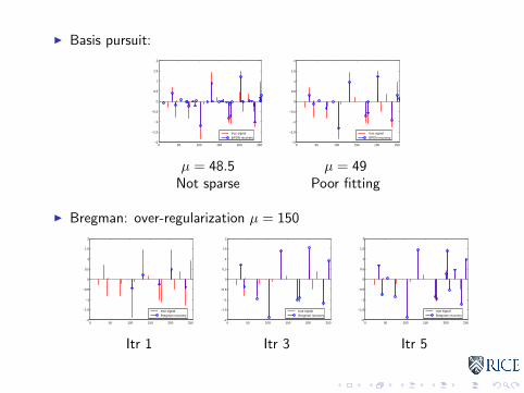
I Basis pursuit:

0 50 100 150 200 250−2

−1.5

−1

−0.5

0

0.5

1

1.5

2

true signalBPDN recovery

µ = 48.5Not sparse

0 50 100 150 200 250−2

−1.5

−1

−0.5

0

0.5

1

1.5

2


µ = 49Poor fitting

I Bregman: over-regularization µ = 150

0 50 100 150 200 250−2

−1.5

−1

−0.5

0

0.5

1

1.5

2

true signalBregman recovery

Itr 1

0 50 100 150 200 250−2

−1.5

−1

−0.5

0

0.5

1

1.5

2


Itr 3

0 50 100 150 200 250−2

−1.5

−1

−0.5

0

0.5

1

1.5

2


Itr 5

I Basis pursuit:

0 50 100 150 200 250−2

−1.5

−1

−0.5

0

0.5

1

1.5

2


µ = 48.5Not sparse

0 50 100 150 200 250−2

−1.5

−1

−0.5

0

0.5

1

1.5

2


µ = 49Poor fitting

I Bregman: over-regularization µ = 150

0 50 100 150 200 250−2

−1.5

−1

−0.5

0

0.5

1

1.5

2


Itr 1

0 50 100 150 200 250−2

−1.5

−1

−0.5

0

0.5

1

1.5

2


Itr 3

0 50 100 150 200 250−2

−1.5

−1

−0.5

0

0.5

1

1.5

2


Itr 5

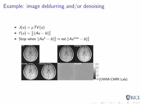
Example: image deblurring and/or denoising

I J(u) = µTV (u)

I f (u) = 12‖Au − b‖22

I Stop when ‖Auk − b‖22 ≈ est.‖Autrue − b‖22

(UWM-CMRI Lab)

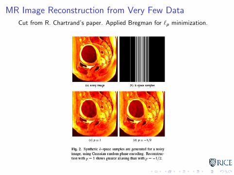
MR Image Reconstruction from Very Few Data

Cut from R. Chartrand’s paper. Applied Bregman for `p minimization.

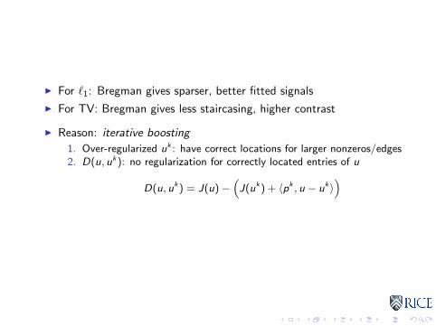
I For `1: Bregman gives sparser, better fitted signals

I For TV: Bregman gives less staircasing, higher contrast

I Reason: iterative boosting

1. Over-regularized uk : have correct locations for larger nonzeros/edges2. D(u, uk): no regularization for correctly located entries of u

D(u, uk) = J(u)−(J(uk) + 〈pk , u − uk〉

)

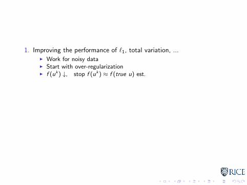
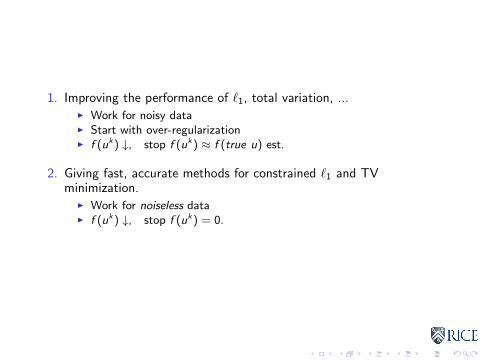
1. Improving the performance of `1, total variation, ...I Work for noisy dataI Start with over-regularizationI f (uk) ↓, stop f (uk) ≈ f (true u) est.

2. Giving fast, accurate methods for constrained `1 and TVminimization.

I Work for noiseless dataI f (uk) ↓, stop f (uk) = 0.

1. Improving the performance of `1, total variation, ...I Work for noisy dataI Start with over-regularizationI f (uk) ↓, stop f (uk) ≈ f (true u) est.

2. Giving fast, accurate methods for constrained `1 and TVminimization.

I Work for noiseless dataI f (uk) ↓, stop f (uk) = 0.

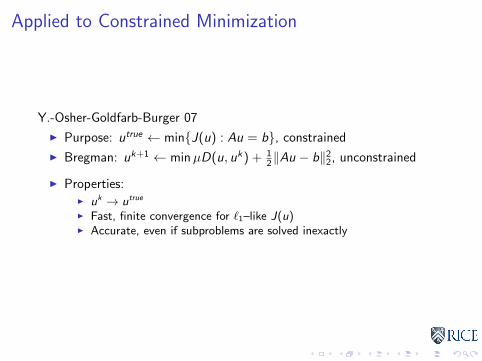
Applied to Constrained Minimization

Y.-Osher-Goldfarb-Burger 07

I Purpose: utrue ← min{J(u) : Au = b}, constrained

I Bregman: uk+1 ← minµD(u, uk) + 12‖Au − b‖22, unconstrained

I Properties:I uk → utrue

I Fast, finite convergence for `1–like J(u)I Accurate, even if subproblems are solved inexactly

However, Bregman iteration has been around since 1967. Moreover, it isequivalent to augmented Lagrangian (when constraints are linear), usedin optimization and computation without great success in e.g.,Navier-Stokes (NS), because NS involves basically L2 minimization.

Bregman turns out to work very well for `1, TV, and relatedminimization; nothing special otherwise.

Reason: Error Cancellation.

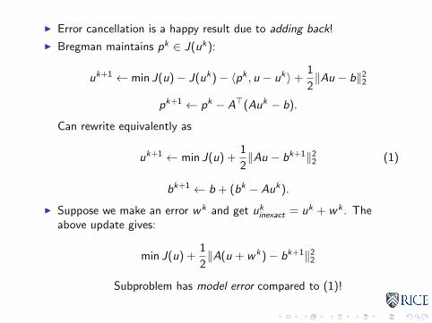
I Error cancellation is a happy result due to adding back!

I Bregman maintains pk ∈ J(uk):

uk+1 ← min J(u)− J(uk)− 〈pk , u − uk〉+1

2‖Au − b‖22

pk+1 ← pk − A>(Auk − b).

Can rewrite equivalently as

uk+1 ← min J(u) +1

2‖Au − bk+1‖22 (1)

bk+1 ← b + (bk − Auk).

I Suppose we make an error wk and get ukinexact = uk + wk . Theabove update gives:

min J(u) +1

2‖A(u + wk)− bk+1‖22

Subproblem has model error compared to (1)!

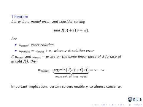
TheoremLet w be a model error, and consider solving

min J(u) + f (u + w).

Let

I uexact : exact solution

I uinexact = uexact + v, where v is solution error

If uexact and uexact − w are on the same linear piece of J (a face ofgraph(J)), then

uinexact − arg min{J(u) + f (u)}︸︷︷︸exact sol. of true model

= v − w .

Important implication: certain solvers enable v to almost cancel w .

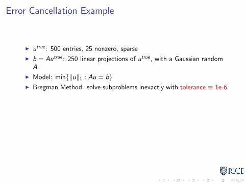
Error Cancellation Example

I utrue : 500 entries, 25 nonzero, sparse

I b = Autrue : 250 linear projections of utrue , with a Gaussian randomA

I Model: min{‖u‖1 : Au = b}I Bregman Method: solve subproblems inexactly with tolerance ≡ 1e-6

Itr k 1 2 3 4 5‖utrue−uk

inexact‖‖utrue‖ 6.5e-2 2.3e-7 6.2e-14 7.9e-16 5.6e-16.

I Above high accuracy obtainable with subproblem solvers:FPC, FPC-BB, GPSR, GPSR–BB, SpaRSA















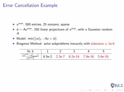
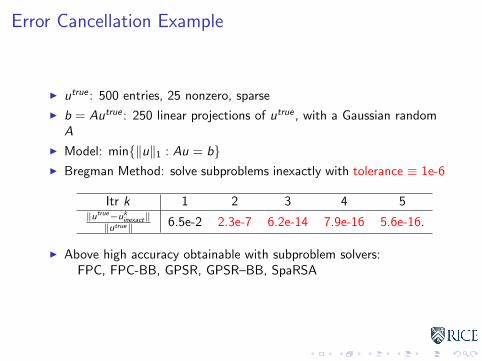
Generalization to Bregman Iterations

I Inverse scale space (Burger, Gilboa, Osher, Xu, etc.)

I Linearized Bregman (Yin, Osher, Mao, etc.)

I Logistic Regression (Shi, et al.)

I Split Bregman (Goldstein, Osher)

I More ... People use the words “Bregmanize” and “Bregmanized”

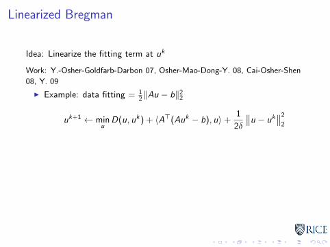
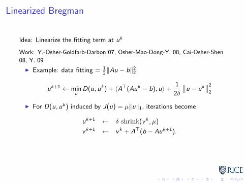
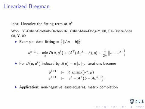
Linearized Bregman

Idea: Linearize the fitting term at uk

Work: Y.-Osher-Goldfarb-Darbon 07, Osher-Mao-Dong-Y. 08, Cai-Osher-Shen

08, Y. 09

I Example: data fitting = 12‖Au − b‖22

uk+1 ← minu

D(u, uk) + 〈A>(Auk − b), u〉+1

2δ

∥∥u − uk∥∥22

I For D(u, uk) induced by J(u) = µ‖u‖1, iterations become

uk+1 ← δ shrink(vk , µ)

vk+1 ← vk + A>(b − Auk+1).

I Application: non-negative least–squares, matrix completion

Linearized Bregman



08, Y. 09


uk+1 ← minu

D(u, uk) + 〈A>(Auk − b), u〉+1

2δ

∥∥u − uk∥∥22



vk+1 ← vk + A>(b − Auk+1).


Linearized Bregman



08, Y. 09


uk+1 ← minu

D(u, uk) + 〈A>(Auk − b), u〉+1

2δ

∥∥u − uk∥∥22



vk+1 ← vk + A>(b − Auk+1).


Linearized Bregman



08, Y. 09


uk+1 ← minu

D(u, uk) + 〈A>(Auk − b), u〉+1

2δ

∥∥u − uk∥∥22



vk+1 ← vk + A>(b − Auk+1).


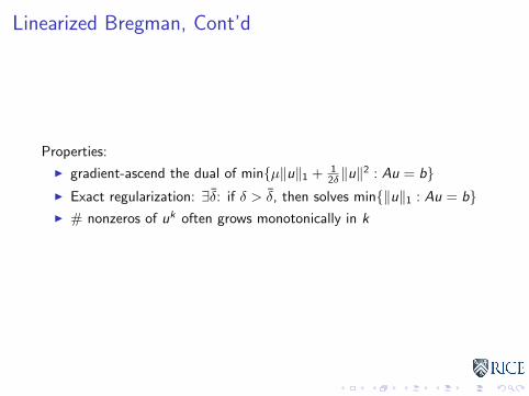
Linearized Bregman, Cont’d

Properties:

I gradient-ascend the dual of min{µ‖u‖1 + 12δ‖u‖

2 : Au = b}I Exact regularization: ∃δ̄: if δ > δ̄, then solves min{‖u‖1 : Au = b}I # nonzeros of uk often grows monotonically in k

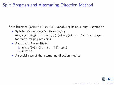
Split Bregman and Alternating Direction Method

Split Bregman (Goldstein–Osher 08): variable splitting + aug. Lagrangian

I Splitting (Wang–Yang–Y.–Zhang 07,08):minu f (Lu) + g(u) =⇒ minu,v{f (v) + g(u) : v = Lu} Great payofffor many imaging problems

I Aug. Lag.: λ – multiplier

1. minu,v f (v) + c2‖v − Lu − λ‖22 + g(u)

2. update λ

I A special case of the alternating direction method

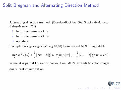
Split Bregman and Alternating Direction Method

Alternating direction method: (Douglas–Rachford 60s, Glowinski–Marocco,

Gabay–Mercier, 70s)

1. fix u, minimize w.r.t. v

2. fix v , minimize w.r.t. u

3. update λ

Example (Wang–Yang–Y.–Zhang 07,08) Compressed MRI, image deblr

minuµTV (u) +

1

2‖Au − b‖22 ⇔ min

u{µ‖w‖1 +

1

2‖Au − b‖22 : w = Du}

where A is partial Fourier or convolution. ADM extends to color images,

duals, rank-minimization

Summary

1. Bregman improves `1-like regularization quality for noisy data

2. Bregman applied to constrained (Au = b) minimization is not newbut is fast and accurate due adding back

3. Various extensions take advantages of model structures

More details and solvers at Rice L1-Related Optimization Project

Documents

The Bregman Methods: Review and New Results - …optimization/L1/bregman/WotaoYin_Bregman... · The Bregman Methods: Review and New Results ... 0 50 100 150 200 250-2-1.5-1-0.5 0