Embed Size (px)
Citation preview

University of California,Santa Barbara
Senior Thesis
Bregman Algorithms
Author:
Jacqueline Bush
Supervisor:
Dr. Carlos
Garcıa-Cervera
June 10, 2011

Acknowledgments
I could not have done this without the help and support of my advisor
Dr. Carlos Garcia-Cervera.
i

Abstract
In this paper we investigate methods for solving the Basis Pursuit problem and
the Total Variation denoising problem. The methods studied here are based on
the Bregman iterative regularization, and efficient algorithm for convex, con-
straint optimization problems. We study two different versions of the original
Bregman iterative algorithm: the Linearized Bregman algorithm, and the Split
Bregman algorithm. We find that the original Bregman Algorithm has good
convergence properties, but while these properties hold for the linearized ver-
sion, they do not always hold for the Split Bregman Algorithm.
ii

iii

Contents
1 Introduction 1
2 Background 4
3 Bregman Iterative Algorithm 8
3.1 Convergence properties of the Bregman Iterative Algorithm . . . 10
4 Linearized Bregman Iterative Algorithm 14
4.1 Linearized Bregman Iterative Algorithm with Kicking . . . . . . 17
5 Split Bregman Algorithm 20
5.1 Anisotropic TV Denoising . . . . . . . . . . . . . . . . . . . . . . 23
5.2 Isotropic TV Denoising . . . . . . . . . . . . . . . . . . . . . . . 26
6 Numerical Results 29
6.1 Basis Pursuit Problem . . . . . . . . . . . . . . . . . . . . . . . . 29
6.2 Image Denoising Problem . . . . . . . . . . . . . . . . . . . . . . 32
7 Further Study 37
8 Matlab Code 38
8.1 Linearized Bregman . . . . . . . . . . . . . . . . . . . . . . . . . 42
8.2 Linear Bregman with kicking . . . . . . . . . . . . . . . . . . . . 42
8.3 Anisotropic TV Denoising . . . . . . . . . . . . . . . . . . . . . . 44
8.4 Isotropic TV Denoising . . . . . . . . . . . . . . . . . . . . . . . 47
iv
List of Figures
1 Linearized Bregman Algorithm . . . . . . . . . . . . . . . . . . . 18
2 Linearized Bregman Algorithm . . . . . . . . . . . . . . . . . . . 20
3 Linearized Bregman Algorithm, m=10, n=30, ||u||0 = 0.1n . . . . 31
4 Linearized Bregman Algorithm, m=50, n=200, ||u||0 = 0.05n . . 31
5 Split Bregman Results using Fluid Jet Image . . . . . . . . . . . 34
6 Split Bregman Error Results using the Fluid Jet Image . . . . . . 34
7 Split Bregman Results using Clown Image . . . . . . . . . . . . . 35
8 Split Bregman Error Results using the Clown Image . . . . . . . 35
9 Split Bregman Results using Durer Detail Image . . . . . . . . . 36
10 Split Bregman Error Results using the Durer Detail Image . . . . 36
v

1 Introduction
In this paper we study Bregman Iterative algorithms, and their ability to solve
constrained optimization problems such as the Basis Pursuit problem and the
Total Variation (TV) denoising problem.
In the Basis Pursuit problem we are interested in finding a solution u ∈ Rn
to the linear system of equations Au = f , where A ∈ Rm×n with m << n, and
f ∈ Rm. We assume that the rows of A are linearly independent. As a result,
the system is underdetermined, and therefore it has infinitely many solutions.
In the Basis Pursuit problem we look for a solution to the linear system of
equations with minimal l1 norm, i.e., we want to solve the constrained problem
minsubject to Au=f ,
‖u‖1, (1.1)
where
||u||1 =n∑
i=1
|ui|. (1.2)
Imposing the constraint in (1.1) leads to a number of difficulties, so instead, we
relax the constraint, and solve the unconstrained basis pursuit problem
minu∈Rn
µ||u||1 +12||Au− f ||22, (1.3)
where µ ∈ R is a positive constant. One can prove that when µ → 0, the solution
to the unconstrained problem converges to a solution of the constrained problem.
The basis pursuit problem appears in applications of compressed sensing,
where a signal assumed to be sparse is reconstructed from incomplete data on it.
Using this principle one can encode a sparse signal u using a linear transforma-
tion Au = f ∈ Rm, and then recover u from f using (1.3). Recent applications
of the basis pursuit problem include compressive imaging, and computer vision
1

tasks to name a few [10].
In our second problem, the TV denoising problem, we want to recover an
image that has been affected by noise. This leads to a problem of the form
minu∈BV (Ω)
||u||BV + H(u), (1.4)
where H(u) is a convex function. The functional in (1.4) is minimized among
functions of bounded variation (BV): Given Ω ⊂ Rn and u : Ω → R, we define
its bounded variation as [4]
||u||BV =sup ∫
Ω
u div(g) dx | g = (g1, g2, · · · , gn) ∈ C10 (Ω, Rn)
and |g(x)| ≤ 1 for x ∈ Ω
,
where
div(g) =n∑
i=1
∂gi
∂xi. (1.5)
The space of functions of bounded variation is defined as BV (Ω) = u : Ω →
R|‖u‖BV < +∞, and it is a Banach space. Notice that if u ∈ C1(Ω), then
integration by parts gives,
‖u‖BV =∫
Ω
|∇u| dx = ‖∇u‖1. (1.6)
Therefore, the Sobolev space W 1,1(Ω) of functions in L1(Ω) whose gradient is in
L1(Ω) is contained in BV (Ω): W 1,1(Ω) ⊂ BV (Ω). However, BV (Ω) 6= W 1,1(Ω):
Consider for instance a set E ⊆ Ω with a smooth boundary, and u = χE , its
characteristic function. Then,
‖χE‖BV = H1(∂E),
2
the surface area of ∂E. However, since χE is discontinuous at the interface ∂E,
∇χE /∈ L1(Ω). This example, which might seem artificial at first, is the typical
situation when one tries to recover an image, since images are best represented
by a collection of disjoint sets, i.e., separated by sharp interfaces. Thus BV (Ω),
and not the Sobolev space W 1,p(Ω) of functions in Lp(Ω) whose gradient is also
in Lp(Ω), seems to be the natural space in which to consider the TV denoising
problem. However, evaluating the BV -norm of a function can be costly, and it
is sometimes replaced by the L1-norm of the gradient. Since the focus in this
thesis is the application of Bregman-type algorithms to this problem, this is the
approach that we will take.
Thus, in the TV denoising problem considered here, we are given as data a
function f ∈ L2(Ω), which is the representation of the noisy image. We try to
recover the original image by minimizing
minu∈BV (Ω)
||∇u||1 +µ
2||u− f ||22, (1.7)
where µ > 0 is a constant. Reducing the noise from obtained images can be ap-
plied to many fields. For example, if we can reduce the noise on images coming
in from a satellite one can save the millions of dollars that it would require to
send an astronaut to repair it. It can also be applied to reduce noise from an
medical test such as an MRI or CT scan.
This thesis is organized as follows: In section 2 we introduce some of the defini-
tions and concepts to be used throughout the remainder of the thesis. In section
3 the Bregman iterative algorithm is introduced and its convergence properties
are studied. A linearized version of the algorithm is derived in section 4. One
drawback of the Linearized Bregman algorithm is that it can reach periods of
stagnation, where progress toward the solution is slow. A method called Kicking
3

that reduces the number of iterations that the algorithm spends in these peri-
ods of stagnation is also described in section 4. In section 5 the Split Bregman
algorithm is introduced and studied. It is shown in section 6 that the Linearized
Bregman algorithm solves the basis pursuit problem quickly and accurately. It
is also shown that the Split Bregman algorithm is not monotonic, unlike the
iterative Bregman algorithm introduced in section 3.
2 Background
Several algorithms have been introduced to solve (1.3), such as the l1ls algo-
rithm developed by S-J. Kim, K. Koh, and S. Boyd [7]. The authors applied an
interior-point method to a log-barrier formulation of (1.3). Each interior point
iteration involved solving a system of linear equations. These iterations were
accelerated using a preconditioned conjugate gradient method, for which S-J.
Kim, K. Koh, and S. Boyd developed an efficient preconditioner [7]. While this
algorithm does solve (1.3), it can be expensive in time and computer memory.
For medium sized problems it can require up to a hundred iterations, but for very
large problems the algorithm could take several hundred iterations to compute
a solution with relative tolerance 0.01 [7]. The Bregman Iterative Algorithms
described in the next sections are proposed as a faster, less computationally
expensive alternative.
In what follows, we consider a normed space X, with norm ‖ · ‖.
Definition A function J : X → R is said to be convex if ∀ x, y ∈ X and any
t ∈ [0, 1],
J(tx + (1− t)y) ≤ tJ(x) + (1− t)J(y). (2.1)
4
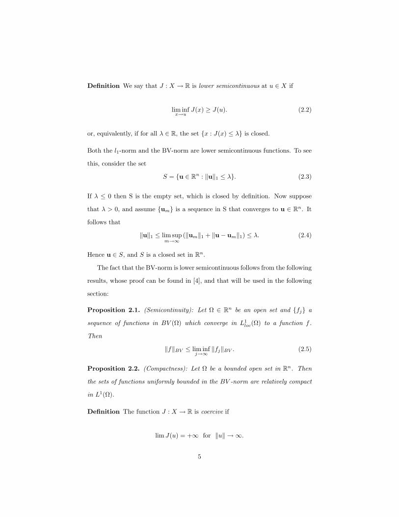
Definition We say that J : X → R is lower semicontinuous at u ∈ X if
lim infx→u
J(x) ≥ J(u). (2.2)
or, equivalently, if for all λ ∈ R, the set x : J(x) ≤ λ is closed.
Both the l1-norm and the BV-norm are lower semicontinuous functions. To see
this, consider the set
S = u ∈ Rn : ‖u‖1 ≤ λ. (2.3)
If λ ≤ 0 then S is the empty set, which is closed by definition. Now suppose
that λ > 0, and assume um is a sequence in S that converges to u ∈ Rn. It
follows that
‖u‖1 ≤ lim supm→∞
(‖um‖1 + ‖u− um‖1) ≤ λ. (2.4)
Hence u ∈ S, and S is a closed set in Rn.
The fact that the BV-norm is lower semicontinuous follows from the following
results, whose proof can be found in [4], and that will be used in the following
section:
Proposition 2.1. (Semicontinuity): Let Ω ∈ Rn be an open set and fj a
sequence of functions in BV (Ω) which converge in L1loc(Ω) to a function f .
Then
‖f‖BV ≤ lim infj→∞
‖fj‖BV . (2.5)
Proposition 2.2. (Compactness): Let Ω be a bounded open set in Rn. Then
the sets of functions uniformly bounded in the BV -norm are relatively compact
in L1(Ω).
Definition The function J : X → R is coercive if
lim J(u) = +∞ for ‖u‖ → ∞.
5
The importance of this definition can be seen from the following
Proposition 2.3. Let V be a reflexive Banach space, and X a non-empty
closed, convex subset of V . Assume that J : X → R is convex, lower semi-
continuous, and coercive. Then, the problem
infu∈X
J(u)
has at least one solution.
The poof can be found in [3].
Definition The dual space of X, denoted by X∗, is defined to be the set of
functions l : X → R such that l is linear and continuous.
Given an element l ∈ X∗, we denote l(u) = 〈l;u〉 for all u ∈ X.
Definition Suppose J : X → R is a convex function and u ∈ X. An element
p ∈ X∗ is called a subgradient of J at u if ∀v ∈ X
J(v)− J(u)− 〈p, v − u〉 ≥ 0. (2.6)
The set of all subgradients of J at u is called the subdifferential of J at u, and
it is denoted by ∂J(u).
Notice that the subdifferential extends the notion of gradient of a function. For
example, consider f(x) = ‖x‖2 in Rn, the Euclidean norm. This function is not
differentiable at x = 0, however it has a subdifferential at x = 0, and in fact
∂f(0) is the closed ball (in the Euclidean norm) around 0 with radius 1, B1(0).
Definition Consider a function J : X → R. We call the limit as λ → 0+, if it
exists, ofJ(u + λv)− J(u)
λ
6

the directional derivative of J at u in the direction v, and denote it by J ′(u; v).
If there exists p ∈ X∗ such that
J ′(u, v) = 〈p, v〉 ∀v ∈ X,
we say that J is Gateaux-differentiable at u, and call p the Gateaux-differential
of J at u, and denote it by J ′(u).
One can prove that if J : X → R is Gateaux-differentiable at u ∈ X, then
∂J(u) = J ′(u). And conversely, if J is continuous at u ∈ X and has only
one subgradient, then J is Gateaux-differentiable at u and ∂J(u) = J ′(u).
In addition notice that J : X → R has a minimum at u ∈ X if and only if
0 ∈ ∂J(u), for in that case
J(v)− J(u) ≥ 〈0, v − u〉 = 0.
Finally, all the algorithms discussed in this paper rely on the Bregman distance,
introduced by L. M. Bregman in 1966 [1].
Definition Suppose J : X → R is a convex function, u, v ∈ X and p ∈ ∂J(v).
Then the Bregman Distance between points u and v is defined by
Dpj (u, v) = J(u)− J(v)− 〈p, u− v〉 . (2.7)
The Bregman distance has several nice properties that make it an efficient tool
to solve l1 regularization problems, such as,
Property 2.4. For all u, v ∈ X, and p ∈ ∂J(v), DpJ(u, v) ≥ 0 .
Proof. Since p ∈ ∂J(v), this property follows directly from the definition of
subdifferentials.
7

Property 2.5. DpJ(v, v) = 0
Proof. Observe, DpJ(v, v) = J(v)− J(v)− < p, 0 >= 0.
Note that in general the Bregman Distance is not symmetric. For instance
if p ∈ ∂J(v)∩ ∈ ∂J(u) then
DpJ(u, v) = J(u)− J(v)− < p, u− v >
= J(u)− J(v)+ < p, v − u >
= −(J(v)− J(u)− < p, v − u >)
= −DpJ(v, u)
3 Bregman Iterative Algorithm
In [8], S. Osher, M. Burger, D. Goldfarb, J. Xu, and W. Yin proposed the
Bregman Iterative Algorithm as an efficient algorithm for solving problems of
the form
minuJ(u) + H(u, f) , (3.1)
where for a closed and convex set X both J : X → R and H : X → R are convex
nonnegative functions with respect to u ∈ X, for a fixed f . In addition H(u, f)
is assumed to be differentiable. Recall f is the vector or matrix, depending on
the problem, that u was encoded into. Osher, Burger, Goldfarb, Xu, and Yin
defined the Bregman iterative algorithm as follows
Bregman Iterative Algorithm:
Initialize: k=0, u0 = 0, p0 = 0
while “uk not converge” do
uk+1 = argminu Dpk
J (u, uk) + H(u)
8

pk+1 = pk −∇H(uk+1) ∈ ∂J(uk+1)
k = k + 1
end while
It is easy to see that the first iteration yields
u1 = minu∈X
(J(u) + H(u)). (3.2)
Hence the first iteration of this algorithm solves (3.1). However to solve our ini-
tial problem we need the residual term to be minimal. This is why the Bregman
Iterative Algorithm continues until the residual term converges.
While working with basis pursuit problems we let J(u) = ||u||1 and H(u) =
12 ||Au− f ||22. When studying image denoising we let J(u) = ||u||BV or J(u) =
‖∇u‖1, and H(u) = ||u− f ||22.
Proposition 3.1. Let X be a reflexive Banach space. The iterative proce-
dure in the above algorithm is well defined if H : X → R and J : X → R
are convex, J is lower semicontinuous and coercive, H is bounded below and
Gateaux-differentiable.
Proof. Since H is bounded below, we can assume that H is nonnegative without
loss of generality. Otherwise, define H = H − inf H. Since H and H differ by
a constant, the algorithm applied to J + H generates the same sequence uk.
The above algorithm is well defined if for each k,
Qk(u) = Dpk−1
J (u, uk−1) + H(u) (3.3)
has a minimizer, uk, and pk = pk−1 − ∇H(uk) ∈ ∂J(uk). Recall that the
9

Bregman Distance and H(u) are nonnegative. Hence,
Qk(u) = J(u)− J(uk−1)−⟨pk−1, u− uk−1
⟩+ H(u)
≥ J(u)− J(uk−1)−⟨pk−1, u− uk−1
⟩= Dpk−1
J (u, uk−1) ≥ 0
It follows that Qk(u) has a lower bound for all k. From the coercivity of J and
the continuity of H, it follows by Prop. 2.3 that Qk(u) has a minimizer, uk, for
each k. Since Qk(u) has a minimum at uk, it follows that 0 ∈ ∂Qk(uk). Hence,
0 ∈ ∂J(uk)− pk−1 +∇H(uk),
⇒ pk−1 −∇H(uk) ∈ ∂J(uk),
⇒ pk ∈ ∂J(uk) ∀k ≥ 1.
Note that if J(u) = ‖u‖BV , then minimizing sequences are precompact,
by Proposition 2.2, and J is lower semicontinuous by Proposition 2.1. The
existence of minimizers follows then from the Direct Method in the Calculus of
Variations [2].
3.1 Convergence properties of the Bregman Iterative Al-
gorithm
The Bregman Iterative Algorithm has been applied to many problems including
image denoising and basis pursuit because it has some very nice convergence
properties. These properties include monotonic decrease in the residual term,
convergence to the original image or signal that we are trying to recover in the
residual term with exact data, and convergence in terms of Bregman distance
10

to the original image or signal with noisy data. We assume that X, J , and H
satisfy the same assumptions as in Proposition 3.1.
In the first result, we show that the sequence generated by the algorithm
monotonically decreases H:
Proposition 3.2. Monotonic decrease in H:
H(uk+1) ≤ H(uk+1) + Dpk
J (uk+1, uk) ≤ H(uk). (3.4)
Proof. Recall that the Bregman distance is nonnegative and that uk+1 mini-
mizes Dpk
J (u, uk) + H(u). Hence
H(uk+1) ≤ H(uk+1) + Dpk
J (uk+1, uk) ≤ H(uk) + Dpk
J (uk, uk) = H(uk).
Next we show that the sequence of residual terms H(uk) converges to the
minimum value of H:
Proposition 3.3. If u minimizes H : X → R and J(u) < ∞, then
H(uk) ≤ H(u) + J(u)/k. (3.5)
11

Proof. Observe that
Dpk
(u, uk) + Dpk−1(uk, uk−1)−Dpk−1
(u, uk−1) =
= J(u)− J(uk)+ < pk, uk − u > +J(uk)− J(uk−1)
+ < pk−1, uk−1 − uk > −J(u) + J(uk−1)− < pk−1, uk−1 − u >
= < pk, uk − u > + < pk−1, uk−1 − uk > − < pk−1, uk−1 − u >
= < pk, uk − u > − < pk−1, uk − u >
= < pk − pk−1, uk − u > .
By construction,
pk − pk−1 = −∇H(uk). (3.6)
Since H is convex it follows that
< pk−1 − pk, uk − u >=< ∇H(uk), uk − u) >≤ H(u)−H(uk). (3.7)
Then we get the following equation:
Dpj
(u, uj) + Dpj−1(uj , uj−1)−Dpj−1
(u, uj−1) ≤ H(u)−H(uj) ∀j. (3.8)
Now if we sum in j in equation (3.8) we get,
k∑j=1
Dpj
(u, uj) + Dpj−1(uj , uj−1)−Dpj−1
(u, uj−1) ≤k∑
j=1
H(u)−H(uj)
⇒ Dpk
(u, uk) +k∑
j=1
[Dpj−1
(uj , uj−1)−H(u) + H(uj)]≤ D0(u, u0) = J(u).
From proposition 3.2 and since the Bregman distance is never negative we can
12

rewrite the above equation as follows,
Dpk
(u, uk) + k[H(uk)−H(u)] ≤ J(u). (3.9)
Hence
H(uk) ≤ H(u) +J(u)
k. (3.10)
Next we show that as long as the residual term H(uk; f) > δ2 then the
Bregman distance between the original signal or image and the current iteration
is decreasing.
Proposition 3.4. For an open set X let H : X → R suppose H(u; f) ≤ δ2 and
H(u; g) = 0 ( f , g, u, δ, represent noisy data, noiseless data, perfect recovery,
and noise level, respectively). Then Dpk+1
J (u, uk+1) < Dpk
J (u, uk) as long as
H(uk+1) > δ2.
Proof. Suppose H(u) < δ2 and insert it into equation (3.8), then
Dpj
(u, uj) + Dpj−1(uj , uj−1)−Dpj−1
(u, uj−1) ≤ δ2 −H(uj)
⇒ Dpj
(u, uj)−Dpj−1(u, uj−1) ≤ δ2 −H(uj).
It follows that if H(uj) > δ2 then
Dpj
(u, uj) ≤ Dpj−1(u, uj−1).
13

4 Linearized Bregman Iterative Algorithm
The Bregman algorithm is a good tool to solve the basis pursuit problem ex-
plained in the introduction. However, at each step the algorithm requires the
minimization of
Dp(u, uk) + H(u), (4.1)
which can be computationally expensive. A linearized version of the Bregman
Iterative Algorithm was introduced by Yin, Osher, Goldfarb and Darbon in [10].
The main advantage of the linearized algorithm is that the minimization of (4.1)
is replaced by a minimization step that can be solved exactly, which allows for
efficient computation. We begin by linearizing H(u): Given uk we approximate
H(u) by,
H(u) = H(uk)+ < ∇H(uk), u− uk > . (4.2)
Since this approximation is only accurate for u close to uk, Yin, Osher, Goldfarb,
and Darbon added the penalty term 12δ ||u−uk||22. The original problem is then
replaced by
uk+1 = arg minu
Dpk
J (u, uk)+H(uk)+ < ∇H(uk), u−uk > +12δ||u−uk||22. (4.3)
Notice that the penalty term also makes the objective function bounded below,
and
||(u− uk) + δ∇H(uk)||2 = ||u− uk||22 + 2δ < ∇H(uk), u− uk > +δ2||H(uk)||22.
In addition, observe that ||H(uk)||22 and H(uk) are constants with respect to u.
It follows that the iteration (4.3) is equivalent to the iteration
uk+1 = arg minu
Dpk
J (u, uk) +12δ||u− (uk − δ∇H(uk))||22. (4.4)
14
We apply this method to the Basis Pursuit problem (1.3), and let H(u) =
12 ||Au− f ||22. Plugging this H into (4.4) we get
uk+1 = arg minu
Dpk
J (u, uk) +12δ||u− (uk − δAT (Auk − f))||22. (4.5)
Now we derive a special case of (4.5). The case when J(u) = µ||u||1 and µ > 0.
In section 3 we defined pk+1 ∈ ∂J(uk+1) by
pk+1 = pk −∇H(uk) (4.6)
= pk − 1δ(uk+1 − (uk − δAT (Auk − f))). (4.7)
Hence,
pk+1 = pk−AT (Auk−f)− (uk+1 − uk)δ
= · · · =k∑
j=0
AT (f−Auj)− uk+1
δ. (4.8)
Let
vk =k∑
j=0
AT (f −Auj). (4.9)
Then,
δvk − δpk+1 = uk+1, (4.10)
⇒ pk = vk−1 − uk
δ. (4.11)
15

Then we get
uk+1 =minu
µ||u||1 − µ||uk||1− < u− uk, pk > +12δ||u− (uk − δAT (Auk − f))||22
=minu
µ
n∑i=1
|ui| − µ||uk||1− < u− uk, vk−1 − uk
δ>
+12δ||u− (uk − δAT (Auk − f))||22
=minu
µ
n∑i=1
|ui|− < u, vk−1 − uk
δ> +
12δ||u− (uk − δAT (Auk − f))||22 + C
Where C denotes constant terms with respect to u ∈ X. Notice that u ∈ X is
componentwise separable. Hence we can minimize each component of u ∈ X
separably. Doing this we get,
0 =
µ− vk−1
i + uki
δ + ui
δ − uki
δ − (AT (f −Auk))i ui > 0
0 ui = 0
µ + vk−1i − uk
i
δ − ui
δ + uki
δ + (AT (f −Auk))i ui < 0
0 =
µ− vk
i + ui
δ ui > 0
0 ui = 0
vki + µ− ui
δ ui < 0
⇒ uk+1i =
δ(vk
i − µ) vki ∈ (µ,∞)
0 vki ∈ [−µ, µ]
δ(vki + µ) vk
i ∈ (−∞,−µ)
For convenience of notation we define the shrinkage function as follows: For
a ≥ 0,
shrink(y, a) =
y − a, y ∈ (a,∞)
0, y ∈ [−a, a]
y + a, y ∈ (−∞,−a)
16

It follows that
uk+1i = δ shrink(vk
i , µ). (4.12)
The linearized algorithm for this special case can then be written as
Linearized Bregman Algorithm:
Initialize: u = 0, v=0
while “||f −Au|| does not converge” do
vk+1 = vk + AT (f −Auk)
uk+1 = δ shrink(vk+1i , µ)
end while
4.1 Linearized Bregman Iterative Algorithm with Kicking
When running the Linearized Bregman iterative algorithm sometimes there ex-
ist periods of stagnation, where the residual stays almost constant for a large
number of iterations. This is illustrated in figure 1, where we solve the Basis
Pursuit problem (1.3) using the Linearized Bregman algorithm. We chose a
random matrix A of size 50× 200, and the number of nonzero elements in the
original signal was 20.
It took Matlab 0.438609 seconds to run the Linearized Bregman iterative algo-
rithm and reduce the initial residual to 0.000932. While the Linearized Bregman
algorithm is already fast, we can make it faster by removing the stagnation pe-
riods seen in figure 1. To get rid of unnecessary iterations we estimate the
number of steps required to leave the stagnation period. Observe that during a
stagnation period of, say, m steps,
uk+j = uk+1,
vk+j = vk + jAT (f −Auk+1) j = 1, · · · ,m.
17
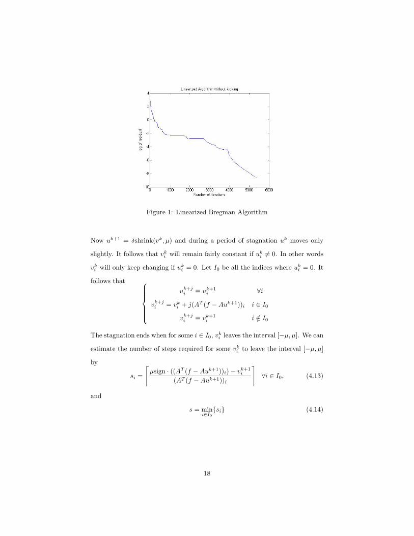
Figure 1: Linearized Bregman Algorithm
Now uk+1 = δshrink(vk, µ) and during a period of stagnation uk moves only
slightly. It follows that vki will remain fairly constant if uk
i 6= 0. In other words
vki will only keep changing if uk
i = 0. Let I0 be all the indices where uki = 0. It
follows that uk+j
i ≡ uk+1i ∀i
vk+ji = vk
i + j(AT (f −Auk+1))i i ∈ I0
vk+ji ≡ vk+1
i i /∈ I0
The stagnation ends when for some i ∈ I0, vki leaves the interval [−µ, µ]. We can
estimate the number of steps required for some vki to leave the interval [−µ, µ]
by
si =
⌈µsign · ((AT (f −Auk+1))i)− vk+1
i
(AT (f −Auk+1))i
⌉∀i ∈ I0, (4.13)
and
s = mini∈I0
si (4.14)
18

Using s we can predict the end of the stagnation period. We define the next
update by uk+s ≡ uk+1
vk+s = vk + sAT (f −Auk+1).
This is the concept of Kicking, introduced by Osher, Moa , Dong, and Yin [9].
The Linearized Bregman iterative algorithm with Kicking is:
Linearized Bregman Iteration with Kicking:
Initialize: u = 0, v = 0
while “||f −Au|| does not converge” do
uk+1 = δshrink(vk, µ)
if “uk+1 ≈ uk” then
calculate s from (4.13) and (4.14)
vk+1i = vk
i + s(AT (f −Auk+1))i, ∀u ∈ I0
vk+1i = vk
i ∀u /∈ I0
else
vk+1 = vk + AT (f −Auk+1)
end if
end while
We ran this algorithm for the same matrix A and original signal u to see if the
kicking method really reduced the number of iterations required to solve (1.3).
It took Matlab 0.065734 seconds to run this algorithm and reduce the initial
residual to 0.000943 for this A and u. Notice that the linearized Bregman
algorithm took less than half of the time the linearized Bregman algorithm
without kicking. The number of iterations required to solve (1.3) also decreased
from 5369 iterations to 665 iterations when we applied kicking.
19

Figure 2: Linearized Bregman Algorithm
5 Split Bregman Algorithm
In [5] T. Goldstein, and S. Osher introduced the Split Bregman method to solve
the general optimization problem of the form
minu∈X
‖Φ(u)‖1 + H(u), (5.1)
where X is a closed, convex set, and both Φ : X → R, and H : X → R
are convex functions. We rewrite (5.1) in terms of the equivalent constrained
minimization problem,
minu∈X,d∈R
‖d‖1 + H(u) such that d = Φ(u). (5.2)
As in the Basis Pursuit problem, we relax the constraints and work with the
unconstrained problem
minu∈X,d∈R
‖d‖1 + H(u) +λ
2||d− Φ(u)||22, (5.3)
20

where λ > 0 is a constant. By defining
J(u, d) = |d|1 + H(u), (5.4)
we can write (5.3) as
minu∈X,d∈R
J(u, d) +λ
2||d− Φ(u)||22. (5.5)
Notice that this is the same problem that we addressed in section 3 with the
iterative Bregman algorithm. We can thus solve (5.5) by using the iterative
Bregman algorithm, which generates the following sequences:
(uk+1, dk+1) = minu∈X,d∈R
DpJ(u, uk, d, dk) +
λ
2||d− Φ(u)||22, (5.6)
pk+1u =pk
u − λ(∇Φ)T (Φ(uk+1)− dk+1), (5.7)
pk+1d =pk
d − λ(dk+1 − Φ(uk+1)). (5.8)
Since the iterative Bregman algorithm is well defined we know that (5.6) has a
minimum and that (pk+1u , pk+1
d ) ∈ ∂J(uk+1, dk+1). Expanding (5.6) we get,
(uk+1, dk+1) = minu∈X,d∈R
J(u, d)− J(uk, dk)− < pku, u− uk > − < pk
d, d− dk >
+λ
2||d− Φ(u)||22. (5.9)
In addition notice that,
pk+1u = pk
u − λ(∇Φ)T (Φ(uk+1)− dk+1) (5.10)
= −λ(∇Φ)Tk+1∑i=1
(Φ(ui)− di), (5.11)
21
and
pk+1d = pk
d − λ(dk+1 − Φ(uk+1)) = λ
k+1∑i=1
(Φ(ui)− di). (5.12)
Define
bk+1 = bk + (Φ(uk+1)− dk+1) =k+1∑i=1
(Φ(ui)− di). (5.13)
Then it follows that
pku = −λ(∇Φ)T bk ∀k ≥ 0, (5.14)
and
pkd = λbk ∀k ≥ 0. (5.15)
Applying (5.14) and (5.15) to (5.9) we get
(uk+1, dk+1) = minu∈X,d∈R
J(u, d)− J(uk, dk) + λ < bk,Φu− Φuk >
− λ < bk, d− dk > +λ
2||d− Φ(u)||22
= minu∈X,d∈R
J(u, d)− J(uk, dk)− λ < bk, d− Φu >
− λ < bk, dk − Φuk > +λ
2||d− Φ(u)||22
= minu∈X,d∈R
J(u, d)− λ < bk, d− Φu > +λ
2||d− Φ(u)||22 + C1
= minu∈X,d∈R
J(u, d) +λ
2||d− Φ(u)− bk||22 + C2, (5.16)
where C1 and C2 are constants. This is the Split Bregman method introduced
by Goldstein and Osher [5], which we write more compactly in the following
form:
Split Bregman Algorithm:
Initialize: k=0, u0 = 0, b0 = 0
22

while ||uk − uk−1||22 >tol do
uk+1 = minu H(u) + λ2 ||d
k − Φ(u)− bk||22
dk+1 = mind |d|+ λ2 ||d− Φ(uk+1)− bk||22
bk+1 = bk + (Φ(uk+1)− dk+1)
k = k + 1
end while
By using the idea in the Split Bregman algorithm, the Bregman algorithm can
be applied to more general optimization problems of the form
minu∈X
J(u) +12||u− f ||22. (5.17)
We apply the Split Bregman Algorithm to the problems of anisotropic TV de-
noising and isotropic TV denoising.
5.1 Anisotropic TV Denoising
We first consider the Anisotropic TV Denoising problem,
minu
∥∥∥∥∂u
∂x
∥∥∥∥1
+∥∥∥∥∂u
∂y
∥∥∥∥1
+µ
2‖u− f‖22, (5.18)
where f is the noisy image. We will will denote ∂u∂x by ux and ∂u
∂y by uy. We
consider the equivalent constrained problem to (5.18)
minu‖dx‖1 + ‖dy‖1 +
µ
2‖u− f‖22, such that dx = ux and dy = uy. (5.19)
As in the previous section to solve (5.19) we actually solve the unconstrained
version
minu,dx,dy
‖dx‖1 + ‖dy‖1 +µ
2‖u− f‖22 +
λ
2‖dx − ux‖22 +
λ
2‖dy − uy‖22. (5.20)
23
Note that this is the same problem that we addressed when deriving the split
Bregman algorithm. We can thus solve (5.20) by using the split Bregman algo-
rithm
(uk+1, dk+1x , dk+1
y ) = minu,dx,dy
‖dx‖1 + ‖dy‖1 +µ
2‖u− f‖22 +
λ
2‖dx − ux − bk
x‖22
+λ
2‖dy − uy − bk
y‖22, (5.21)
bk+1x =bk
x + (uk+1x − dk+1
x ), (5.22)
bk+1y =bk
y + (uk+1y − dk+1
y ). (5.23)
Notice that the functional being minimized in the first step is smooth with
respect to u. To minimize it we simply set its first variational derivative equal
to zero:
0 = µ(uk+1 − f)− λ∇Tx (dk
x − uk+1x − bk
x)
−λ∇Ty (dk
y − uk+1y − bk
y), (5.24)
= µuk+1 − µf − λ∇Tx (dk
x − bkx) + λuk+1
xx + λuk+1yy
−λ∇Ty (dk
y − bky), (5.25)
⇒ (µI + λ∆)uk+1 = µf + λ∇Tx (dk
x − bkx) + λ∇T
y (dky − bk
y). (5.26)
This problem is solved using Dirichlet boundary conditions. For our examples
we choose Ω to be a rectangular domain, and discretize the equations using
a uniform grid. We approximate the partial derivatives using second order,
centered finite differences. The terms of the form ‖d‖pp are approximated by
‖d‖pp ≈ ∆x∆y
∑|di,j |p.
24

Following [5], we solve the system of equations using the Gauss-Seidel iteration.
Faster methods could also be used, such as the Conjugate Gradient Method,
or Multigrid [6]. The Gauss-Seidel solution can be written componentwise as
follows:
uk+1i,j = Gk
i,j =λ
µ + 4λ(uk
i+1,j + uki−1,j + uk
i,j+1 + uki,j−1 + dk
x,i−1,j − dkx,i,j
+ dky,i,j−1 − dk
y,i,j − bkx,i−1,j + bk
x,i,j − bky,i,j−1 + by,i,j)
+µ
µ + 4λfi,j . (5.27)
At the boundaries of the domain we used one-sided finite differences instead of
the centered finite differences. Next we solve the problem with respect to dx.
Since the function f(x) = |x| is differentiable in R\0, when we minimize with
respect to dx, we get:
0 =
1 + λdk
x − λuk+1x − λbk
x dkx > 0
0 dkx = 0
1− λdkx + λuk+1
x + λbkx dk
x < 0
⇒ dkx =
(uk+1
x + bkx)− 1
λ (uk+1x + bk
x) ∈(
1λ ,∞
)0 (uk+1
x + bkx) ∈
[− 1
λ , 1λ
]1λ + uk+1
x + bkx (uk+1
x + bkx) ∈
(−∞,− 1
λ
)= shrink
(uk+1
x + bkx,
1λ
).
Now observe that the equation for dy is the same as the equation for dx, and
can be obtained by replacing all the x′s by y′s. It follows then that
dky = shrink
(uk+1
y + bky ,
1λ
). (5.28)
25

Therefore the Split Bregman Anisotropic TV Denoising algorithm can be writ-
ten as follows:
Split Bregman Anisotropic TV Denoising:
Initialize: k=0, u0 = 0, b0 = 0
while ||uk − uk−1||22 >tol do
uk+1 = Gk where G is the Gauss-Seidel function defined earlier.
dk+1x = shrink
(∇xuk+1 + bk
x, 1λ
)dk+1
y = shrink(∇yuk+1 + bk
y , 1λ
)bk+1x = bk
x + (∇xuk+1 − dk+1x )
bk+1y = bk
y + (∇yuk+1 − dk+1y )
k = k + 1
end while
5.2 Isotropic TV Denoising
In the Isotropic TV model we solve the following problem:
minu||∇u||2 +
µ
2||u− f ||22. (5.29)
We rewrite this problem as a constrained problem,
minu||(dx, dy)||2 +
µ
2||u− f ||22, such that dx = ux and dy = uy, (5.30)
and as in the previous section we relax the constraints and solve the uncon-
strained problem
minu,dx,dy
||(dx, dy)||2 +µ
2||u− f ||22 +
λ
2||dx − ux||22 +
λ
2||dy − uy||22. (5.31)
26

Note that this is the same problem that we addressed when deriving the split
Bregman algorithm. We can thus solve (5.31) by using the split Bregman algo-
rithm
(uk+1, dk+1x , dk+1
y ) = minu,dx,dy
||(dx, dy)||2 +µ
2||u− f ||22 +
λ
2||dx − ux − bk
x||22
+λ
2||dy − uy − bk
y ||22, (5.32)
bk+1x = bk
x + (uk+1x − dk+1
x ), (5.33)
bk+1y = bk
y + (uk+1y − dk+1
y ). (5.34)
The minimization problem with respect to u in the first step is the same as
in the Anisotropic problem. Hence as before we let uk+1 = Gk where Gk is
the Gauss-Seidel solution given in equation (5.27). The difference between the
Anisotropic problem and the isotropic problem lies in how we calculate dx and
dy. Unlike the anisotropic problem, in the isotropic problem dx and dy are
coupled together. Consider the minimization problem with respect to dx,
0 =dk+1
x
||(dkx, dk
y)||2+ λ(dk+1
x − ukx − bk
x). (5.35)
(5.36)
Define
sk =√|uk
x + bkx|2 + |uk
y + bky |2. (5.37)
27

We approximate ||(dkx, dk
y)||2 by sk, which leads to
0 =dk+1
x
sk+ λ(dk+1
x − ukx − bk
x)
⇒ dk+1x
(λ +
1sk
)= λ(uk
x + bkx)
=skλ(uk
x + bkx)
skλ + 1.
As in the previous algorithm dy has the same formula as dx expect the x′s
become y′s, i.e.,
dk+1y =
skλ(uky + bk
y)skλ + 1
.
From this we get the algorithm.
Split Bregman Isotropic TV Denoising:
Initialize: k=0, u0 = 0, b0 = 0
while ||uk − uk−1||22 >tol do
uk+1 = Gk where G is the Gauss-Seidel function defined earlier.
dk+1x = skλ(uk
x+bkx)
skλ+1
dk+1y = skλ(uk
x+bkx)
skλ+1
bk+1x = bk
x + (uk+1x − dk+1
x )
bk+1y = bk
y + (uk+1y − dk+1
y )
k = k + 1
end while
28

6 Numerical Results
6.1 Basis Pursuit Problem
In our numerical experiments we used random matrices generated in Matlab
using randn(m,n). We had Matlab generate random sparse vectors u. We chose
those vectors such that the number of nonzero entries were equal to 0.1n or
0.05n which were obtained using the routine calls round(0.1n) and round(0.05n)
in MATLAB, respectively. We then defined f = Au. The stopping criterion
||Auk − f ||2‖f‖2
< 10−5 (6.1)
was used. In the following tables we show the size of the random matrix A,
the l1 norm of the original vector u, the l1 norm of our solution, the residual
error, the number of iterations required, and the time needed to perform the
algorithm:
Results of linearized Bregman-l1 without kicking
||u||1 ||u||1 ||Au− f ||2 Num. of iter. Time required
m n Number of nonzero entries in u: 0.1n
10 30 1.193162 1.177883 0.000084 17472 0.869771 s
50 100 5.020869 5.020832 0.000712 2334 0.144548 s
50 200 8.173409 6.962439 0.000674 4425 0.306456 s
75 150 6.774425 6.774392 0.000995 296 0.031358 s
m n Number of nonzero entries in u: 0.05n
10 30 0.549661 0.549658 0.000030 820 0.031979 s
50 100 2.130546 2.130546 0.000484 312 0.026888 s
50 200 4.417850 4.417829 0.000808 993 0.068624 s
75 150 4.318850 4.318850 0.000762 74 0.008143 s
29

Results of linearized Bregman-l1 with kicking
||u||1 ||u||1 ||Au− f ||2 Num. of iter. Time required
m n Number of nonzero entries in u: 0.1n
10 30 1.193162 1.178426 0.000083 3970 0.219367 s
50 100 5.020869 5.020938 0.000786 1273 0.104327 s
50 200 8.173409 7.017613 0.000656 786 0.075189 s
75 150 6.774425 6.774426 0.001033 570 0.051384 s
m n Number of nonzero entries in u: 0.05n
10 30 0.549661 0.549660 0.000032 733 0.039978 s
50 100 2.130546 2.130540 0.000338 49 0.006380 s
50 200 4.417850 4.473151 0.000860 11909 1.103843 s
75 150 4.318850 4.318843 0.000829 34 0.005658 s
From the table we can conclude that in general the linearized Bregman algo-
rithm with kicking yields a result that is almost as good as the result yielded
with the linearized Bregman algorithm but with fewer iterations. The following
should be observed: Both the linearized Bregman algorithm, and the linearized
Bregman algorithm with kicking are accurate with a small residual error. The
linearized Bregman algorithm always returns u such that ||u||1 is smaller than
||u||1, but in three of the eight tests the linearized Bregman algorithm with kick-
ing yielded a result u with ||u||1 larger than ||u||1. Furthermore observe that in
most of the tests, the algorithm with kicking solved the problem in significantly
less iterations.
In figures 3 and 4, we plot the residual in the corresponding iterations.
30
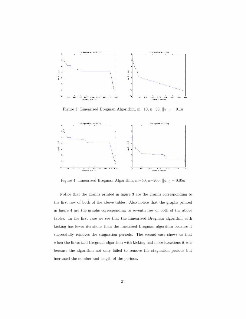
Figure 3: Linearized Bregman Algorithm, m=10, n=30, ||u||0 = 0.1n
Figure 4: Linearized Bregman Algorithm, m=50, n=200, ||u||0 = 0.05n
Notice that the graphs printed in figure 3 are the graphs corresponding to
the first row of both of the above tables. Also notice that the graphs printed
in figure 4 are the graphs corresponding to seventh row of both of the above
tables. In the first case we see that the Linearized Bregman algorithm with
kicking has fewer iterations than the linearized Bregman algorithm because it
successfully removes the stagnation periods. The second case shows us that
when the linearized Bregman algorithm with kicking had more iterations it was
because the algorithm not only failed to remove the stagnation periods but
increased the number and length of the periods.
31

6.2 Image Denoising Problem
To test the algorithms in the TV denoising problem, we considered several
images, added noise to it, and tried to recover from it the original image. We
obtained our images from a list of images already available in Matlab. Suppose
that X is the matrix representation of an image, of size m×n. To add noise to
X we created a random matrix N using the Matlab command rand(m,n). We
then defined our noisy image to be f = X + cN , where c > 0 is a constant.
For our experiments we used µ = 0.1, λ = 0.2, c = 20, and tolerance = 10−3.
In tables 1 and 2 we show the results for the Anisotropic and Isotropic TV
denoising algorithms, respectively. The relative error is measured by ||u−X||22.
Image Size Anisotropic TV Denoisingn m Number of Iterations Relative Error Time (s)
Fluid Jet 400 300 15 0.066469 45.265365 sBone 367 490 13 0.050428 57.263076 s
Gatlinburg 480 640 9 0.034703 70.699119 sDurer 648 509 6 0.024618 53.494445 s
Durer Detail 359 371 10 0.084235 33.669978 sCape Cod 360 360 14 0.061195 44.381875 s
Clown 200 320 11 0.086670 17.690584 sEarth 257 250 10 0.071599 16.257617 s
Mandrill 480 500 5 0.030040 33.262180 s
Table 1: Results for the Anisotropic TV denoising algorithm
32
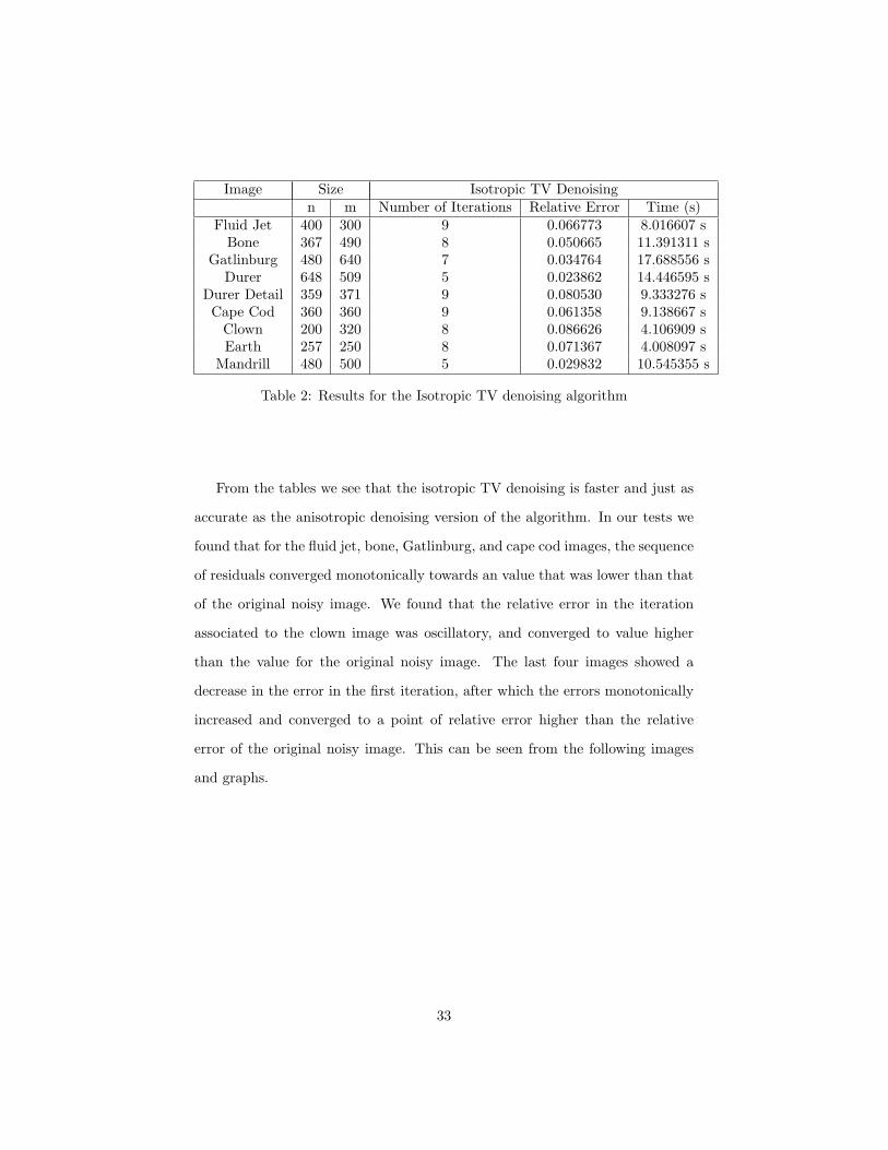
Image Size Isotropic TV Denoisingn m Number of Iterations Relative Error Time (s)
Fluid Jet 400 300 9 0.066773 8.016607 sBone 367 490 8 0.050665 11.391311 s
Gatlinburg 480 640 7 0.034764 17.688556 sDurer 648 509 5 0.023862 14.446595 s
Durer Detail 359 371 9 0.080530 9.333276 sCape Cod 360 360 9 0.061358 9.138667 s
Clown 200 320 8 0.086626 4.106909 sEarth 257 250 8 0.071367 4.008097 s
Mandrill 480 500 5 0.029832 10.545355 s
Table 2: Results for the Isotropic TV denoising algorithm
From the tables we see that the isotropic TV denoising is faster and just as
accurate as the anisotropic denoising version of the algorithm. In our tests we
found that for the fluid jet, bone, Gatlinburg, and cape cod images, the sequence
of residuals converged monotonically towards an value that was lower than that
of the original noisy image. We found that the relative error in the iteration
associated to the clown image was oscillatory, and converged to value higher
than the value for the original noisy image. The last four images showed a
decrease in the error in the first iteration, after which the errors monotonically
increased and converged to a point of relative error higher than the relative
error of the original noisy image. This can be seen from the following images
and graphs.
33
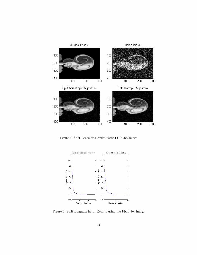
Figure 5: Split Bregman Results using Fluid Jet Image
Figure 6: Split Bregman Error Results using the Fluid Jet Image
34
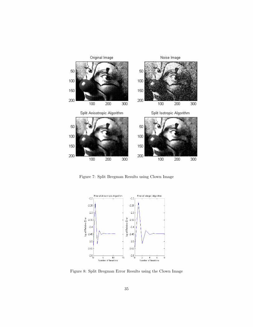
Figure 7: Split Bregman Results using Clown Image
Figure 8: Split Bregman Error Results using the Clown Image
35

Figure 9: Split Bregman Results using Durer Detail Image
Figure 10: Split Bregman Error Results using the Durer Detail Image
36

We showed in section 3.1 that the relative error of the iterative Bregman
algorithm decreased monotonically. However the last two images displayed in
this paper show that the relative error of the Split Bregman algorithm with both
isotropic and anisotropic filters does not necessarily converge monotonically. We
do not currently have a satisfactory explanation for this behavior, and it would
be interesting to explore it further. We would also like to see if other properties
of convergence discussed in section 3.1 hold for the Split Bregman algorithm.
7 Further Study
When experimenting with these algorithm we observed several surprising re-
sults. In the linearized algorithms we noticed that occasionally the linearized
algorithm without kicking performed better than the algorithm with kicking. It
would be interesting to run more tests and experiment with different conditions
to figure out why this happens, and if there was a way to correct this problem.
In addition we would like to investigate why in two of our tests the kicking
version of the linearized algorithm yielded long stagnation periods.
In the image denoising problem the logarithm of the relative error did not al-
ways converge to a point below the initial error. Five of the nine images tested
had this problem. In the future we would like to run more tests and see if
by changing µ and λ we can fix this problem. We would also want to investi-
gate mathematically why the split Bregman algorithm proved not to be strictly
monotonic.
37
8 Matlab Code
The following Matlab codes were written to implement the Linearized Breg-
man Iterative Algorithm, and the Linearized Bregman Iterative Algorithm with
kicking.
function lineartest
clc; clear all;
m=50; n=200;
tic
%Calculate random matrix
A = randn(m,n);
%Code for Sparse Vector (u bar)
nz=round(0.05*n); %Number of nonzero numbers
z=n-nz; %Number of zero numbers
ub= rand(n,1); %Vector of Random Elements
b=randperm(n); %Random Permutation Vector of m elements.
ub(b(1:z))=0 ; %Uses the permutation vector to find z random places,
%and sets them equal to zero.
%Calculate f
f = A*ub;
fprintf(’Linear Algorithm \n’)
[k,u,r] = LinAlgorithm(A,f,n);
fprintf(’Number of Iterations=%.0f\n’,k);
fprintf(’||u||_1=%f\n’, norm(u,1));
fprintf(’||ub||_1= %f\n’, norm(ub,1));
fprintf(’||Au-f||_1 = %f\n’, norm(A*u-f,1));
figure(1)
38
i=(1:k);
plot(i,r(i))
title(’Linear Algorithm with out kicking’)
xlabel(’Number of Iterations’)
ylabel(’log of residual’)
fprintf(’Linear Algorithm with Kicking\n’);
[l,k,u,r]=LinAlgKicking(A,f,n);
fprintf(’Number of times going into if statement=%.0f\n’,l);
fprintf(’Number of Iterations=%.0f\n’,k);
fprintf(’||u||_1=%f\n’, norm(u,1));
fprintf(’||ub||_1= %f\n’, norm(ub,1));
fprintf(’||Au-f||_1 = %f\n’, norm(A*u-f,1));
figure(2)
i=(1:k);
plot(i,r(i))
title(’Linear Algorithm with kicking’ )
xlabel(’Number of Iterations’)
ylabel(’log of residual’)
end
I used the following code to run the Anisotropic and Isotropic TV denoising
codes,
function imagetest
clc; clf; clear all;
clear X map;
imglist = ’flujet’, ... Fluid Jet
’spine’, ... Bone
39

’gatlin’, ... Gatlinburg
’durer’, ... Durer
’detail’, ... Durer Detail
’cape’, ... Cape Cod
’clown’, ... Clown
’earth’, ... Earth
’mandrill’, ... Mandrill
’spiral’;
load(imglist8,’X’,’map’);
c=20; %As c increases the noise in the image gets worse.
noise=randn(size(X));
f=X+c*noise;
mu=.1;lambda=.2; Tol=10^(-3);
size(X)
fprintf(’Split Anisotropic Algorithm \n’)
[u1,l,k]=SplitAnisotropic2(f,X, Tol,lambda, mu);
fprintf(’Number of iterations %0.f \n’,k-1)
p = norm(u1-X,2)/norm(X,2);
fprintf(’Relative error, ||u-X||_2/||X||_2 = %f \n’, p )
fprintf(’Split Isotropic Algorithm \n’)
[u2,ll,kk] = SplitIsotropic2(f,X,Tol,lambda,mu);
pp = norm(u2-X,2)/norm(X,2);
fprintf(’Number of iterations %.0f \n’, kk-1)
fprintf(’Relative error, ||u-X||_2/||X||_2 = %f \n’, pp)
40

figure(1)
colormap(’gray’)
subplot(2,2,1)
image(X)
title(’Original Image’)
subplot(2,2,2)
image(f)
title(’Noise Image’)
subplot(2,2,3)
image(u1)
title(’Split Anisotropic Algorithm’)
subplot(2,2,4)
image(u2)
title(’Split Isotropic Algorithm’)
figure(2)
subplot(1,2,1)
j=(1:k);
plot(j-1, log(l(j)))
xlabel(’Number of Iterations’)
ylabel(’log of Relative Error’)
title(’Error of Anisotropic Algorithm’)
subplot(1,2,2)
i=[1:kk];
41

plot( i-1, log(ll(i)))
xlabel(’Number of Iterations’)
ylabel(’log of Relative Error’)
title(’Error of Istropic Algorithm’)
8.1 Linearized Bregman
The following code implements the linear bregman iterative algorithm,
function [k,u,r]=LinAlgorithm(A,f,n)
tic
%Initialize
u=zeros(n,1); v = zeros(n,1);
delta=.01; mu=1000; epsilon=10^(-5);
%Algorithm
k=0;
while (norm(f-A*u,2)/norm(f,2))>epsilon %stoping criterion
k=k+1;
v = v + A’*(f-A*u);
u = delta*shrink(v,mu);
r(k) = log(norm(f-A*u,2));
end
toc
end
8.2 Linear Bregman with kicking
The following code implements the linear bregman iterative algorithm with kick-
ing,
function [l,k,u,r]=LinAlgKicking(A,f,n)
42

tic
%Initialize
u=zeros(n,1); u1=zeros(n,1); v = A’*(f-A*u);
delta=.01; mu=100; epsilon=10^(-5);
%Algorithm
k=0; l=0; o=0;
while (norm(f-A*u,2)/norm(f,2))>epsilon %stoping criterion
k=k+1;
u1=u;
u = delta*shrink(v,mu);
if norm(abs(u-u1),2)<10^(-8) ;
l= l +1 ;
x=A’*(f-A*u);
for i=1:n
if abs(u(i)) < 10^(-10)
s(i,1)= ceil((mu*sign(x(i))-v(i))/x(i));
else
s(i,1) = 10^(100);
end
end
ss= min(s);
if ss==10^(100)
ss= 1;
end
for i=1:n
if abs(u(i))<10^(-10)
v(i) = v(i) + ss*x(i);
43

else
v(i) = v(i) ;
end
end
else
v = v + A’*(f-A*u);
end
r(k) = log(norm(f-A*u,2));
if k>3 & norm(abs(u-u1),2)<10^(-10)
break
end
end
toc
end
8.3 Anisotropic TV Denoising
The following code implements the split Bregman Algorithm for Anisotropic
TV denoising.
function [u,p,k]=SplitAnisotropic2(f,X,Tol,lambda,mu)
tic
n=size(f,1); m=size(f,2);
n1=n-1; m1=m-1;
u=f; dx =zeros(n,m); dy=zeros(n,m); bx=zeros(n,m); by=zeros(n,m); k=0;
nn(1) = norm(u,2); p(1) = norm(f-X,2)/norm(X,2);
while nn(k+1) >Tol
k=k+1;
u1 = u ;
44

%Calculate u.
for i=2:n1
for j=2:m1
u(i,j)= g(u,dx,dy, bx, by,f, lambda, mu, i,j);
end
end
%Compute the ds
for i=2:n1
for j=1:m
dx(i,j) = shrink((u(i+1,j)- u(i-1,j))/2+bx(i,j),1/lambda);
end
end
for j=1:m
dx(1,j) = shrink((u(1+1,j)- u(1,j))+bx(1,j),1/lambda);
end
for j=1:m
dx(n,j) = shrink((u(n,j)- u(n-1,j))+bx(n,j),1/lambda);
end
for j=2:m1
for i=1:n
dy(i,j) = shrink((u(i,j+1) - u(i,j-1))/2 +by(i,j),1/lambda);
end
end
for i=1:n
dy(i,1) = shrink((u(i,2) - u(i,1)) +by(i,1),1/lambda);
end
for i=1:n
45
dy(i,m) = shrink((u(i,m) - u(i,m-1)) +by(i,m),1/lambda);
end
%Calculate the b’s
for i=2:n1
for j=1:m
bx(i,j) = bx(i,j) + (u(i+1,j)-u(i-1,j))/2 - dx(i,j) ;
end
end
for j=1:m
bx(1,j) = bx(1,j) + (u(1+1,j)-u(1,j)) - dx(1,j) ;
end
for j=1:m
bx(n,j) = bx(n,j) + (u(n,j)-u(n-1,j)) - dx(n,j) ;
end
for i=1:n
for j=2:m1
by(i,j) = by(i,j) + (u(i,j+1)-u(i,j-1))/2 - dy(i,j) ;
end
end
for i=1:n
by(i,1) = by(i,1) + (u(i,1+1)-u(i,1)) - dy(i,1) ;
end
for i=1:n
by(i,m) = by(i,m) + (u(i,m)-u(i,m-1)) - dy(i,m) ;
end
nn(k+1) = norm(u-u1,2)/norm(u,2);
nn(k); nn(k+1);
46

p(k+1)= norm(u-X,2)/norm(X,2);
end
toc
end
8.4 Isotropic TV Denoising
The following matlab code implements the split Bregman algorithm for isotropic
TV denoising.
function [u,p,k]=SplitIsotropic2(f,X,Tol, lambda,mu)
tic
n=size(f,1); m=size(f,2);
n1=n-1; m1=m-1;
u=f; dx =zeros(n,m); dy=zeros(n,m); bx=zeros(n,m); by=zeros(n,m);
k=0; p(1) = norm(f-X,2)/norm(X,2);nn(1) = norm(u,2);
while nn(k+1) >Tol
k=k+1;
u1 = u ;
for i=2:n1
for j=2:m1
u(i,j)= g(u,dx,dy, bx, by,f, lambda, mu, i,j);
end
end
%Compute the sx’s
for i=2:n1
for j=2:m1
s(i,j) = sqrt( abs( (u(i+1,j)-u(i-1,j))/2 + bx(i,j))^2
+ abs((u(i,j+1)-u(i,j-1))/2 + by(i,j))^2);
47
end
end
for i=1:n1
j=1;
s(i,j) = sqrt( abs( (u(i+1,j)-u(i,j)) + bx(i,j))^2
+ abs((u(i,j+1)-u(i,j)) + by(i,j))^2);
end
for j=1:m1
i=1;
s(i,j) = sqrt( abs( (u(i+1,j)-u(i,j)) + bx(i,j))^2
+ abs((u(i,j+1)-u(i,j)) + by(i,j))^2);
end
for i=2:n
j=m;
s(i,j) = sqrt( abs( (u(i,j)-u(i-1,j)) + bx(i,j))^2
+ abs((u(i,j)-u(i,j-1)) + by(i,j))^2);
end
for j=2:m
i=n;
s(i,j) = sqrt( abs( (u(i,j)-u(i-1,j)) + bx(i,j))^2
+ abs((u(i,j)-u(i,j-1)) + by(i,j))^2);
end
for j=1:m1
i=1;
s(i,j) = sqrt( abs( (u(i+1,j)-u(i,j)) + bx(i,j))^2
+ abs((u(i,j+1)-u(i,j)) + by(i,j))^2);
end
48

%Compute the d’s
for i=2:n1
for j=1:m
dx(i,j)= (s(i,j)*lambda*((u(i+1,j)-u(i-1,j))/2+bx(i,j)))
/(s(i,j)*lambda + 1);
end
end
for j=1:m
i=1;
dx(i,j)= (s(i,j)*lambda*((u(i+1,j)-u(i,j))+bx(i,j)))
/(s(i,j)*lambda + 1);
end
for j=1:m
i=n;
dx(i,j)= (s(i,j)*lambda*((u(i,j)-u(i-1,j))+bx(i,j)))
/(s(i,j)*lambda + 1);
end
for i=1:n
for j=2:m1
dy(i,j) = (s(i,j)*lambda*(((u(i,j+1)-u(i,j-1))/2 + by(i,j))))
/(s(i,j)*lambda +1 );
end
end
for i=1:n
j=1;
dy(i,j) = (s(i,j)*lambda*(((u(i,j+1)-u(i,j)) + by(i,j))))
/(s(i,j)*lambda +1 );
49
end
for i=1:n
j=m;
dy(i,j) = (s(i,j)*lambda*(((u(i,j)-u(i,j-1))/2 + by(i,j))))
/(s(i,j)*lambda +1 );
end
%Compute the b’s
for i=2:n1
for j=1:m
bx(i,j)= bx(i,j) + ((u(i+1,j)-u(i-1,j))/2 - dx(i,j));
end
end
for j=1:m
i=1;
bx(i,j)= bx(i,j) + ((u(i+1,j)-u(i,j)) - dx(i,j));
end
for j=1:m
i=n;
bx(i,j)= bx(i,j) + ((u(i,j)-u(i-1,j)) - dx(i,j));
end
for i=1:n
for j=2:m1
by(i,j) = by(i,j) + ((u(i,j+1)-u(i,j-1))/2 - dy(i,j));
end
end
for i=1:n
j=1;
50

by(i,j) = by(i,j) + ((u(i,j+1)-u(i,j)) - dy(i,j));
end
for i=1:n
j=m;
by(i,j) = by(i,j) + ((u(i,j)-u(i,j-1)) - dy(i,j));
end
nn(k+1) = norm(u-u1,2)/norm(u,2);
p(k+1)= norm(u-X,2)/norm(X,2);
end
toc
end
51

References
[1] L. M. Bregman. A relaxation method of finding a common point of convex
sets and its application to the solution of problems in convex programming.
Z. Vycisl. Mat. i Mat. Fiz., 7:620–631, 1967.
[2] Bernard Dacorogna. Introduction to the calculus of variations. Imperial
College Press, London, second edition, 2009. Translated from the 1992
French original.
[3] Ivar Ekeland and Roger Temam. Convex analysis and variational prob-
lems, volume 28 of Classics in Applied Mathematics. Society for Industrial
and Applied Mathematics (SIAM), Philadelphia, PA, english edition, 1999.
Translated from the French.
[4] Enrico Giusti. Minimal surfaces and functions of bounded variation, vol-
ume 80 of Monographs in Mathematics. Birkhauser Verlag, Basel, 1984.
[5] Tom Goldstein and Stanley Osher. The split Bregman method for L1-
regularized problems. SIAM J. Imaging Sci., 2(2):323–343, 2009.
[6] Arieh Iserles. A first course in the numerical analysis of differential equa-
tions. Cambridge Texts in Applied Mathematics. Cambridge University
Press, Cambridge, second edition, 2009.
[7] Kwangmoo Koh, Seung-Jean Kim, and Stephen Boyd. An interior-point
method for large-scale l1-regularized logistic regression. J. Mach. Learn.
Res., 8:1519–1555 (electronic), 2007.
[8] Stanley Osher, Martin Burger, Donald Goldfarb, Jinjun Xu, and Wotao
Yin. An iterative regularization method for total variation-based image
restoration. Multiscale Model. Simul., 4(2):460–489 (electronic), 2005.
52

[9] Stanley Osher, Yu Mao, Bin Dong, and Wotao Yin. Fast linearized Breg-
man iteration for compressive sensing and sparse denoising. Commun.
Math. Sci., 8(1):93–111, 2010.
[10] Wotao Yin, Stanley Osher, Donald Goldfarb, and Jerome Darbon. Bregman
iterative algorithms for l1-minimization with applications to compressed
sensing. SIAM J. Imaging Sci., 1(1):143–168, 2008.
53