The Assignment and Division of the Tax Base in a System of Hierarchical Governments

William H. Hoyt

CESIFO WORKING PAPER NO. 5801 CATEGORY 1: PUBLIC FINANCE

MARCH 2016

An electronic version of the paper may be downloaded • from the SSRN website: www.SSRN.com • from the RePEc website: www.RePEc.org

• from the CESifo website: Twww.CESifo-group.org/wp T

ISSN 2364-1428

CESifo Working Paper No. 5801

The Assignment and Division of the Tax Base in a System of Hierarchical Governments

Abstract Vertical externalities, changes in one level of government’s policies that affect the budget of another level of government, may lead to non-optimal government policies. These externalities are associated with tax bases that are shared or “co-occupied” by two levels of government. Here I consider whether the co-occupancy of tax bases is desirable. I examine the optimal extent of the tax bases of a lower level of government (local) and a higher level (state). I find that it is optimal to have co-occupancy in the absence of other corrective policies if commodities in tax base are substitutes. Further, if the state government can differentially tax the co-occupied segment of the tax base and the segment it alone taxes it will obtain the (second-best) outcome obtained with other policy instruments such as intergovernmental grants. Finally, if there are horizontal externalities generated by cross-border shopping, there is still reason to co-occupy the tax base if commodities are substitutes. As well, local governments should have those commodities with the lowest cross-border shopping costs in their tax base.

JEL-Codes: H200, H710, H730, R120, R280, R410.

Keywords: fiscal competition, vertical externalities, tax base co-occupancy.

William H. Hoyt Department of Economics

Gatton College of Business and Economics University of Kentucky

USA – Lexington, KY 40506 whoyt@uky.edu

This Version: February 2016 Thanks to David Agrawal, Robert Inman, participants at the 2015 National Tax Association meetings, and the University of Kentucky Department of Economics workshop.

1 Introduction

While the concept of a horizontal fiscal externality arising from tax competition among

governments at the same level has been the topic of numerous papers in for more than

thirty years, the focus on “vertical” fiscal externalities received later attention. Among the

early theoretical contributions were Johnson (1988) and Flowers (1988) and continued with

Dahlby (1996, 2008), Boadway and Keen (1996), Boadway, Marchand and Vigneault (1998).

More recent contributions include Boadway, Cuff and Marchand (2003), Keen (1998), Keen

and Kotsogiannis (2002, 2003, 2004), Hoyt (2001), Dahlby and Wilson (2003), Wrede (1996,

2000), Keen and Kotsogiannis (2002), and Wilson and Janeba (2005) among others.

As the name vertical implies, these externalities arise between governments at different

levels, for example, between state and local governments or federal and state governments.

In this case the focus is on the overlap in the tax bases of two levels of government. An

example from Dahlby (1996) is the excise tax placed on cigarettes by both the federal and

state governments in the United States. When choosing its tax rate, each state presumably

only considers the tax’s impact on its own revenues and ignores the impact on the revenues

of other states and the federal government. As a result of an increase in the state’s tax

rate, other states tax revenues will increase because of cross-border shopping (a horizontal

externality) and federal tax revenues will be reduced because of the reduction in the cigarettes

purchases, part of their tax base (a vertical externality). Because of these impacts on the

revenues of other governments, the cost of funds perceived by the state differs from the social

cost of the funds. While the horizontal fiscal externality is positive, the vertical externality is

negative as increases in the state tax reduce federal revenues. Because the state government

ignores this negative externality, it will overtax cigarettes.

A number of studies have considered policies by the higher level of government to cor-

rect for the vertical externalities created by taxes imposed by the lower level of government.

Corrective policies include separating the tax bases of the two levels of government (Flowers

(1988)); increasing the number of lower-level governments (Keen (1995); Keen and Kotso-

giannis (2004)); and providing intergovernmental grants (Dahlby (1996); Boadway and Keen

(1996); Boadway, Marchand and Vigneault (1998); and Flochel and Madies (2002)).

While early studies focused on vertical externalities in a single market, research has

extended to consider the impacts of co-occupancy in a multiple market including studies by

Dahlby (1996), Keen (1998), Hoyt (2001), Dahlby, Mintz and Wilson (2000), and Dahlby

(2001), and Dahlby and Wilson (2003). While I also examine tax policies in a hierarchical

system of governments, I depart from previous studies in a several respects. First I consider

vertical externalities with multiple tax bases. Specifically, I consider a large number (a

2

continuum) of commodities to be included in either or both of levels of governments tax

bases. The consideration of multiple commodities enables us to address the question of

central interest to this paper – how should the tax base be allocated between the two levels

of government?

Vertical fiscal externalities act in both directions – state taxes affect local revenues and

local taxes affect state revenues. Flowers (1988), Wrede (1996), and Keen and Kotsogiannis

(2002), for example, assume that both levels of government ignore the vertical externality

imposed on the other level of government when setting tax policies. This leads to excessive

taxation at both levels of government. Here, I consider both the case in which the state

government considers the impact of its tax policies on local revenues as well as the case in

which it does not. Figure 1 illustrates the fiscal externality imposed by an increase of a local

tax on state government revenues.

In addition to having multiple tax bases, different levels of governments rely on very

different sources of revenue. As Table 1 suggestions, while there is only limited overlap or

co-occupancy in sources of revenue of state and local governments in the United States, for

example, there is likely to be a strong link between their alternative tax bases. Changes

in a major source of state revenue such as the personal income tax will undoubtedly affect

revenues from the property tax, a major local source of revenue. In contrast, there is much

more apparent co-occupancy of the federal and state tax bases primarily because the personal

income tax and, to a lesser extent, the corporate income tax are major sources of tax revenue

for both levels of government. Thus, while vertical fiscal externalities will almost certainly

arise in a co-occupied tax base, it does not follow that eliminating co-occupancy eliminates

fiscal externalities, an idea that may underlie the recommendation by some to eliminate co-

occupancy. In fact, eliminating co-occupancy may change the fiscal externality from being

negative to being positive if the commodities in the two tax bases are substitutes. This, in

turn, would suggest under-taxation rather than over-taxation in the framework developed

here.

The issue addressed here, what level of government should tax what goods or services

or inputs is referred to in the federalism literature as the “assignment” problem. In a

surprisingly small literature, the best known discussion of the appropriate assignment of the

tax base in a system of hierarchical governments may be found in Musgrave (1983) with

nice summaries in Musgrave and Musgrave (1989), Oates (1994), Keen (1998) and Dahlby

(2001). While Musgrave provided some general guidelines for assigning tax bases based on

the elasticity of alternative tax bases, he does not discuss how vertical fiscal externalities

might affect assignment. Keen (1998) does devote some discussion (and analysis) to co-

occupancy and assignment by addressing the question of whether it is better to co-occupy

3

an inelastic tax base or a more elastic tax base. Dahlby (2001) raises several concerns with

Musgrave’s rules for assignment including the issue of co-occupancy. While not presenting

any formal model, Dahlby (2001), by highlighting the general interdependency of tax bases,

raises questions similar to those I address here. In very different contexts both Haufler

and Lulfesmann (2015) and Kotsogiannis and Raimondos (2015) consider “optimal” co-

occupancy. However, in both cases, the co-occupancy corrects for horizontal externalities:

in the case of Haufler and Lulfesmann (2015) these are associated with capital taxation by

asymmetric countries and in the case of Kotsogiannis and Raimondos (2015) countries levy

taxes to change the terms of trade.

An extensive literature on the possible efficacy of co-occupancy has addressed issues re-

lated to horizontal fiscal externalities and cross-jurisdictional trade distortions as a result of

lower-level government tax policies. Perhaps the most extensive discussion of the tax assign-

ment issue has been related to the VAT taxation and the issue of source versus destination

taxation. Contributions to this literature include Bird (2000); Bird and Gendron (1998,

2000); Keen (2000) and Keen and Smith (2000). Recent related contributions to notion of

higher-level government taxation “correcting” for inefficiencies associated with lower-level

government policies include Haufler and Lulfesmann (2015) and Kotsogiannis and Raimon-

dos (2015).

Here I address the assignment question using a very different framework from those in

either Musgrave (1983) or Keen (1998) but similar in many ways to the framework implicit

in Dahlby (2001). Rather than considering the type of tax base that should be taxed by

different levels of government, I first consider how to divide a uniform tax base among two

levels of government and whether co-occupancy is desirable or not. While this very simple

framework means that I ignore many of the issues associated with tax assignment such as

geography, benefit taxation, and cross-border shopping discussed in, for example, Bird (2000)

and McLure (2001) it allows for focus on the question of whether the existence of vertical

fiscal externalities might, as suggested by Flowers (1988) and Dahlby (2001) among others,

lead to the conclusion that there should be no or very limited co-occupancy among tax bases.

Even when the elimination of co-occupancy may be optimal, it does not, in general, eliminate

vertical fiscal externalities. As a consequence, even in the absence of co-occupancy the tax

rates of the two levels of government will not be optimally set. If the commodities in the tax

base are gross substitutes, eliminating co-occupancy results in a positive fiscal externality,

meaning that tax rates will become “too” low. Here, because both the tax rates and tax

bases of governments are policy instruments, I need to distinguish between fiscal externalities

associated with changes in a government’s tax rate and one associated with changes in its

tax base. While the division of the tax base obviously influences the vertical externalities

4

associated with the tax rates, the extent and direction of the fiscal externalities associated

with tax increases and those associated with increases in tax bases can be quite different.

In fact, I find that in the case in which commodities are gross substitutes, co-occupancy,

at least to some extent, is optimal; when commodities are gross complements, it is unlikely

that co-occupancy is optimal.

The basic model, found in Section 2, is of a continuum of commodities with identical

demands along the lines, for example, of Dixit and Stiglitz (1977), Yitzhaki (1979), and

Wilson (1989). In this section I motivate the optimal policies with regard to both the tax

rate and base by considering the policy undertaken by a single, central government that

finances two public services with separate taxes. I then consider the alternative extreme

– the choices of tax rates and tax bases made by the two levels of government (state and

local) when they choose them independently. As I assume that commodities are identical

both governments will set uniform tax rates on their respective bases.1 In Section 3 the

optimal tax bases (from their perspective) for the two levels of government is considered.

In this section I first consider the question of how to divide the tax base between the two

levels of government in the absence of any overlap. I then consider whether and under what

conditions, would co-occupancy be socially optimal. As well, I allow for the possibility that

the state government can set different tax rates on the base that it alone taxes and the base

that it shares (co-occupies) with the local government. Finally, in Section 4 I extend the

model to generate a horizontal externality. In this case, along the lines of Agrawal (2012) and

Nielsen (2001), for example, I allow for cross-border shopping. In addition to generating a

horizontal externality, as I allow for differences in the costs of cross-border shopping among

commodities, I can also address the question of what commodities might be included in

the state and local tax bases rather than simply the extent of the two bases and whether

co-occupancy is optimal. Section 5 concludes.

2 Tax Choices with Independent Governments

2.1 A Simple Model

I consider an economy with a single state government and n local governments with each

locality having a single, identical resident. Each government provides a public service to its

residents with gs being the level provided by the state government and gj, j = 1, ..., n the

1Further assumptions regarding the elasticity of the demands of the products are necessary for this resultas will be seen later. Alternatively, that there are uniform tax rates across commodities can also be consideredan assumption reflecting (most) state and local sales tax in the United States and VAT systems elsewhereas discussed in ?.

5

level provided by locality j. Both public services are produced with constant costs with the

cost of providing gs to the n localities equal to ngs and the cost of providing the local public

service in locality j equal to gj. While there are n independent localities, as each local

government has the same policy objectives, in equilibrium all localities choose the same

policies. Then given this symmetry, I denote local policies by the subscript l. To further

simplify the analysis, I also assume that the number of localities is large enough so that no

individual locality considers the impacts its policies have on state revenues.

In addition to the public services, residents also consume private commodities. Following

Dixit and Stiglitz (1977), Yitzhaki (1979), and Wilson (1989), I consider a continuum of

these private commodities identified on the interval [0,K]. While the interval of commodities

is [0,K] only the interval [0,1] is subject to taxation by either the state or local governments.2

As my interest is in how to allocate the tax base between the two levels of government, like

Dixit and Stiglitz (1977) I assume identical demand functions over the set of commodities.

By this I mean that when the prices of two commodities are identical, the quantity demanded

is the same for both. The utility function can be represented by

U =

K̂

0

(Ux(x(q(k), Q)) dk + U l (gl) + U s (gs) (2.1)

The gross of tax price of commodity k, x(k), is denoted by q(k) with the net of tax prices for all

commodities equal to unity. The term Q =(´ K

0q(k)dk

)is an index of all commodity prices.

Unlike Dixit and Stiglitz (1977), I assume a relatively general form of the utility function.

As the demand function for commodities are identical then when the price of commodity i

and commodity j are the same, their demands are the same. I denote the derivatives of the

demand equations by x11 ≡ ∂x(k)∂q(k)

and x21 ≡ ∂x(k)∂Q

and, what will be used when characterizing

tax rates, the percentage change in demands, x̂11 ≡ ∂x(k)∂q(k)

1x(k)

and x̂21 ≡ ∂x(k)∂Q

1x(k)

that I treat

as constant in the analysis. For my purposes, an important implication of having identical

commodities is that the optimal tax structure is extremely simple – all commodities should

be taxed equally.

As both the local and state governments assess uniform commodity taxes to finance their

public services, the gross price of each commodity depends on whether it is part of the tax

base for the local, state, or both governments. Localities tax the set of commodities on the

interval[0, k̄l

]while the set taxed by the state government is on the interval

[ks, 1

]. Let

kl, ks, and kls denote, respectively, the length of interval taxed only be the local government,

2While we may think of the commodity space as a straight line or circle, like Dixit and Stiglitz (1977) thedistance between any two commodities has no bearing on the relationship between them, that is, the degreeto which they are substitutes or complements. This is seen in the formulation of the price index.

6

only by the state government, and by both levels of government. Then the gross of tax price

for the commodities can be summarized by

q(k) =

1 + τl,

1 + τs,

1 + τl + τs,

k ∈ 0,[min

(kl, ks

))k ∈

[max

(kl, ks

), 1]

k ∈[ks, kl

]if , kl > ks

(2.2)

where τl and τs denote the local and state tax rates respectively.3 Figure 2 illustrates the

division of the tax base with no overlap (no co-occupancy) and with overlap (co-occupancy).

Then the indirect utility function can be expressed as4

V[τl, τs, ks, kl

]=

ˆ K

0

V (q(k), Q) dk + U s(gs(τl, τk, ks, kl

))+ U l

(gl(τl, τk, ks, kl

)). (2.3)

2.1.1 Government Objectives

The objective function for local governments is given by

W l[τl, τs, kl, ks

]=

ˆ K

0

V (q(k), Q)dk + U l(gl(τl, τs, kl, ks

))(2.4)

where the level of the local public service is implicitly defined by the state and local tax

rates and bases, gl(τl, τs, kl, ks

). As local governments are assumed to ignore the impact of

their policies on state revenues, state public services are not included as an argument in the

local government’s welfare functions.

3With these taxes the price index is

Q =

´ ks0

(1 + τl) dk +´ klks

(1 + τl + τs) dk +´ 1kl

(1 + τs) dk +´K1dk

= K + klτl + ksτs + kls (τl + τs)´ kl0

(1 + τl) dk +´ kskldk +

´ 1ks

(1 + τs) dk +´K1dk

= K + klτl + ksτs

.

kl > ks

kl < ks

4where the term

ˆ 1

0

V (q(k), Q) dk =

´ kl0Ux (x(q(k) = 1 + τl, Q)) dk +

´ ksklUx (x(q(k) = 1, Q)) dk

+´ 1ksUx (x(q(k) = 1 + τs, Q)) dk +

´K1Ux (x(q(k) = 1, Q)) dk

, kl < ks

´ ks0Ux (x(q(k) = 1 + τl, Q)) dk +

´ ksklUx (x(q(k) = 1 + τl + τs, Q)) dk

+´ 1ksUx (x(q(k) = 1 + τs, Q)) dk +

´K1Ux (x(q(k) = 1, Q)) dk

, kl > ks

.

7

For the state government consider the objective,

W s[τl, τs, kl, ks

]=

ˆ K

0

V (q(k), Q)dk + U s(gs(τl, τs, ks, kl)) + αU l(gl(τl, τs, ks, kl)) (2.5)

where α ∈ [0, 1]. The parameter α denotes the extent that the state government considers

the impacts of its policies on the local government revenues. If α = 1 the state government

fully considers the impacts of its policies on local revenues and the welfare of its residents;

at the other extreme (α = 0) the state ignores the impacts of its policies on local revenues

and public services. My interest will be focused on these two extreme cases.

2.1.2 Government Budget Constraints

The state budget constraint is given by ngs = nτs (ksxs + klsxls) = nτsXs and the local

budget constraint is given by gl = τl (klxl + klsxls) = τlXl where xs, xl, and xls denote the

demand for commodities subject to the state tax only, to the local tax only, and to both

taxes, respectively.

Critical to understanding the tax rates chosen by the two levels of government and the

optimal tax bases for them is understanding the impacts of changes in their tax rates and

bases on their revenues. These impacts, summarized below, are derived in Appendix A.1.

dgjdτj

= Xj [1 + τj (x̂11 + (kj + kls) x̂21)] and

dgidτj

= τ iXi

[kls

(kls+ki)xlsxix̂11 + (kj + kls) x̂21

], i, j =, ls; i 6= j

(2.6)

where xi = klsxls+kixikls+ki

, i = l, s. Note that the sign and magnitude of the fiscal externalities,dgidτj, i, j = l, s; i 6= j depend on both the overlap in the tax based (kls) and cross-price effects

(x̂21). While the focus of the literature on fiscal externalities has been on tax rates, I am

also interested in the impacts of changes in tax bases of the two levels of government. Then

the impacts of increases in the tax base on revenues are

dgjdkj

= τjxj

[xzxj

+ τl (kls + kj) x̂21

]and dgi

dkj= τjτixi

[D xi

xjx̂11 + (kls + ki) x̂21

], i, j = l, s; i 6= j,

(2.7)

where D = 0 (1) and z = j(ls) if kl < (>) ks, j = l, s .5 As is the case with tax rates,

changes in the tax bases of the two levels of government affect tax revenues of the other level

of government. The impact of the expansion of the tax base by one level of government on

the other levels tax revenue depends on whether the two tax bases overlap and the cross-price

5An increase in the state tax base means a decrease in ks so rather than dgsdks

and dgldks

(2.7) is for − dgsdks

and − dgldks

.

8

elasticities (impacts) among commodities, relative to their own price elasticities – when the

two tax bases overlap, increases in the local (state) tax base will always decrease the state

(local) tax base.

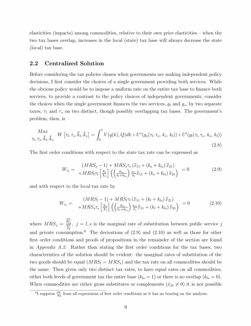
2.2 Centralized Solution

Before considering the tax policies chosen when governments are making independent policy

decisions, I first consider the choices of a single government providing both services. While

the obvious policy would be to impose a uniform rate on the entire tax base to finance both

services, to provide a contrast to the policy choices of independent governments, consider

the choices when the single government finances the two services, gl and gs, by two separate

taxes, τ l and τ s on two distinct, though possibly overlapping tax bases. The government’s

problem, then, is

Max

τl, τs, kl, ksW[τl, τs, kl, ks

]=

ˆ 1

0

V (q(k), Q)dk+U s(gs(τl, τs, ks, kl)) +U l(gl(τl, τs, ks, kl))

(2.8)

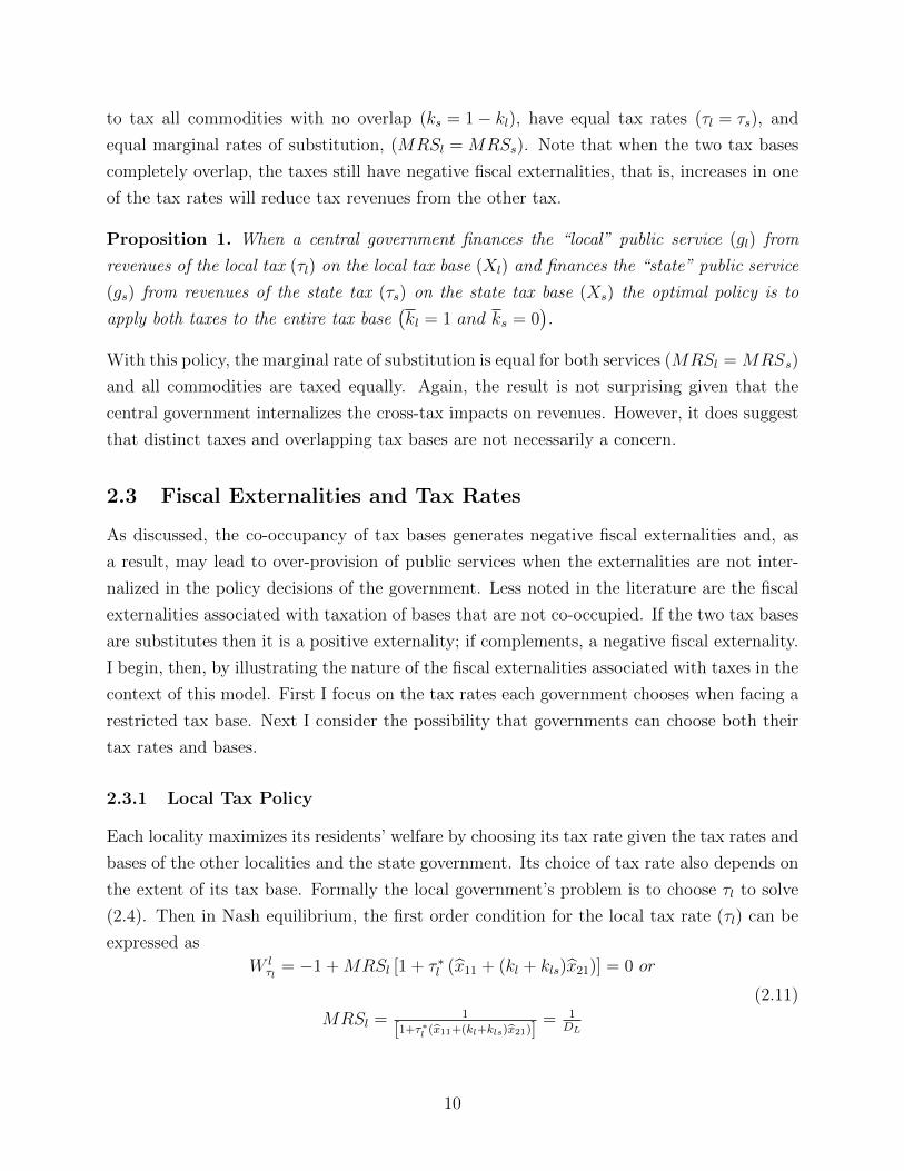
The first order conditions with respect to the state tax rate can be expressed as

Wτl =(MRSs − 1) +MRSsτs (x̂11 + (ks + kls) x̂21)

+MRSlτl

[XlXs

] ((kls

kl+kls

)xlsxlx̂11 + (ks + kls) x̂21

) = 0 (2.9)

and with respect to the local tax rate by

Wτs =(MRSl − 1) +MRSlτl (x̂11 + (kl + kls) x̂21)

+MRSsτs

[XsXl

] ((kls

ks+kls

)xlsxsx̂11 + (kl + kls) x̂21

) = 0 (2.10)

where MRSj =∂V∂gj∂V∂y

, j = l, s is the marginal rate of substitution between public service j

and private consumption.6 The derivations of (2.9) and (2.10) as well as those for other

first order conditions and proofs of propositions in the remainder of the section are found

in Appendix A.2. Rather than stating the first order conditions for the tax bases, two

characteristics of the solution should be evident: the marginal rates of substitution of the

two goods should be equal (MRSl = MRSs) and the tax rate on all commodities should be

the same. Then given only two distinct tax rates, to have equal rates on all commodities,

either both levels of government tax the entire base (kls = 1) or there is no overlap (kls = 0).

When commodities are either gross substitutes or complements (x̂21 6= 0) it is not possible

6I suppress ∂V∂y from all expressions of first order conditions as it has no bearing on the analysis.

9

to tax all commodities with no overlap (ks = 1− kl), have equal tax rates (τl = τs), and

equal marginal rates of substitution, (MRSl = MRSs). Note that when the two tax bases

completely overlap, the taxes still have negative fiscal externalities, that is, increases in one

of the tax rates will reduce tax revenues from the other tax.

Proposition 1. When a central government finances the “local” public service (gl) from

revenues of the local tax (τl) on the local tax base (Xl) and finances the “state” public service

(gs) from revenues of the state tax (τs) on the state tax base (Xs) the optimal policy is to

apply both taxes to the entire tax base(kl = 1 and ks = 0

).

With this policy, the marginal rate of substitution is equal for both services (MRSl = MRSs)

and all commodities are taxed equally. Again, the result is not surprising given that the

central government internalizes the cross-tax impacts on revenues. However, it does suggest

that distinct taxes and overlapping tax bases are not necessarily a concern.

2.3 Fiscal Externalities and Tax Rates

As discussed, the co-occupancy of tax bases generates negative fiscal externalities and, as

a result, may lead to over-provision of public services when the externalities are not inter-

nalized in the policy decisions of the government. Less noted in the literature are the fiscal

externalities associated with taxation of bases that are not co-occupied. If the two tax bases

are substitutes then it is a positive externality; if complements, a negative fiscal externality.

I begin, then, by illustrating the nature of the fiscal externalities associated with taxes in the

context of this model. First I focus on the tax rates each government chooses when facing a

restricted tax base. Next I consider the possibility that governments can choose both their

tax rates and bases.

2.3.1 Local Tax Policy

Each locality maximizes its residents’ welfare by choosing its tax rate given the tax rates and

bases of the other localities and the state government. Its choice of tax rate also depends on

the extent of its tax base. Formally the local government’s problem is to choose τl to solve

(2.4). Then in Nash equilibrium, the first order condition for the local tax rate (τl) can be

expressed as

W lτl

= −1 +MRSl [1 + τ ∗l (x̂11 + (kl + kls)x̂21)] = 0 or

MRSl = 1

[1+τ∗l (x̂11+(kl+kls)x̂21)]= 1

DL

(2.11)

10

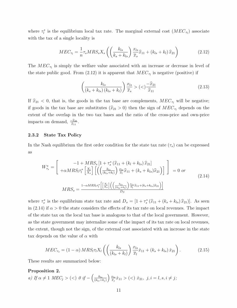
where τ ∗l is the equilibrium local tax rate. The marginal external cost (MECτl) associate

with the tax of a single locality is

MECτl =1

nτsMRSsXs

((kls

ks + kls

)xlsxsx̂11 + (kls + kl) x̂21

)(2.12)

The MECτl is simply the welfare value associated with an increase or decrease in level of

the state public good. From (2.12) it is apparent that MECτl is negative (positive) if(kls

(ks + kls) (kls + kl)

)xlsxs

> (<)−x̂21x̂11

(2.13)

If x̂21 < 0, that is, the goods in the tax base are complements, MECτl will be negative;

if goods in the tax base are substitutes (x̂21 > 0) then the sign of MECτl depends on the

extent of the overlap in the two tax bases and the ratio of the cross-price and own-price

impacts on demand, −x̂21x̂11

.

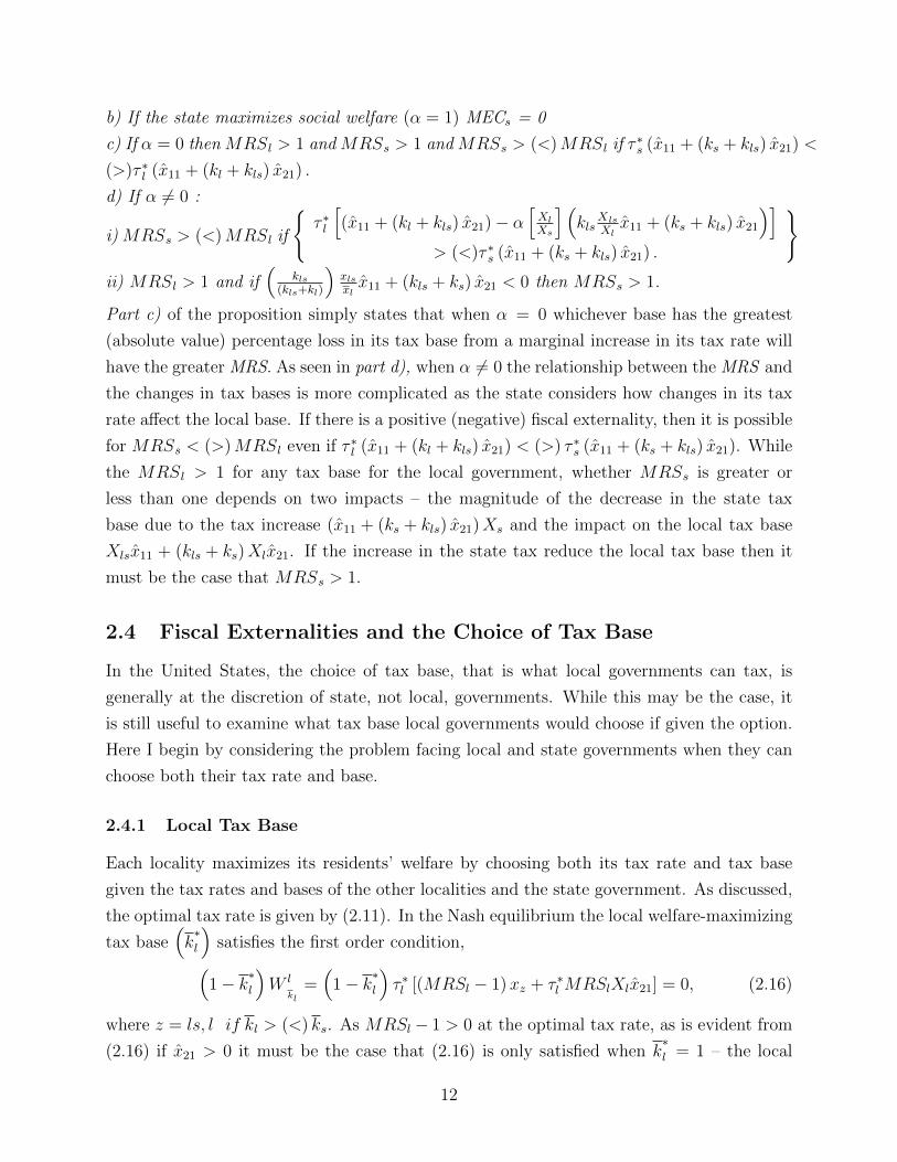
2.3.2 State Tax Policy

In the Nash equilibrium the first order condition for the state tax rate (τs) can be expressed

as

W sτs =

[−1 +MRSs [1 + τ ∗s (x̂11 + (kl + kls) x̂21]

+αMRSlτ∗l

[XlXs

] [((kls

(kls+kl)

)xlsxlx̂11 + (ks + kls)x̂21

)] ]= 0 or

MRSs =1−αMRSlτ

∗l

[[XlXs

]((kls

(kls+kl)

)xlsxlx̂11+(ks+kls)x̂21

)]DS

(2.14)

where τ ∗s is the equilibrium state tax rate and Ds = [1 + τ ∗s (x̂11 + (ks + kls) x̂21)]. As seen

in (2.14) if α > 0 the state considers the effects of its tax rate on local revenues. The impact

of the state tax on the local tax base is analogous to that of the local government. However,

as the state government may internalize some of the impact of its tax rate on local revenues,

the extent, though not the sign, of the external cost associated with an increase in the state

tax depends on the value of α with

MECτs = (1− α)MRSlτlXl

((kls

(kls + kl)

)xlsxlx̂11 + (ks + kls) x̂21

). (2.15)

These results are summarized below:

Proposition 2.

a) If α 6= 1 MECj > (<) 0 if −(

kls(kls+kj)

)xlsxjx̂11 > (<) x̂21, j, i = l, s, i 6= j;

11

b) If the state maximizes social welfare (α = 1) MECs = 0

c) If α = 0 then MRSl > 1 and MRSs > 1 and MRSs > (<)MRSl if τ ∗s (x̂11 + (ks + kls) x̂21) <

(>)τ ∗l (x̂11 + (kl + kls) x̂21) .

d) If α 6= 0 :

i) MRSs > (<)MRSl if

{τ ∗l

[(x̂11 + (kl + kls) x̂21)− α

[XlXs

] (kls

Xls

Xlx̂11 + (ks + kls) x̂21

)]> (<)τ ∗s (x̂11 + (ks + kls) x̂21) .

}ii) MRSl > 1 and if

(kls

(kls+kl)

)xlsxlx̂11 + (kls + ks) x̂21 < 0 then MRSs > 1.

Part c) of the proposition simply states that when α = 0 whichever base has the greatest

(absolute value) percentage loss in its tax base from a marginal increase in its tax rate will

have the greater MRS. As seen in part d), when α 6= 0 the relationship between the MRS and

the changes in tax bases is more complicated as the state considers how changes in its tax

rate affect the local base. If there is a positive (negative) fiscal externality, then it is possible

for MRSs < (>)MRSl even if τ ∗l (x̂11 + (kl + kls) x̂21) < (>) τ ∗s (x̂11 + (ks + kls) x̂21). While

the MRSl > 1 for any tax base for the local government, whether MRSs is greater or

less than one depends on two impacts – the magnitude of the decrease in the state tax

base due to the tax increase (x̂11 + (ks + kls) x̂21)Xs and the impact on the local tax base

Xlsx̂11 + (kls + ks)Xlx̂21. If the increase in the state tax reduce the local tax base then it

must be the case that MRSs > 1.

2.4 Fiscal Externalities and the Choice of Tax Base

In the United States, the choice of tax base, that is what local governments can tax, is

generally at the discretion of state, not local, governments. While this may be the case, it

is still useful to examine what tax base local governments would choose if given the option.

Here I begin by considering the problem facing local and state governments when they can

choose both their tax rate and base.

2.4.1 Local Tax Base

Each locality maximizes its residents’ welfare by choosing both its tax rate and tax base

given the tax rates and bases of the other localities and the state government. As discussed,

the optimal tax rate is given by (2.11). In the Nash equilibrium the local welfare-maximizing

tax base(k∗l

)satisfies the first order condition,(

1− k∗l)W l

kl

=(

1− k∗l)τ ∗l [(MRSl − 1)xz + τ ∗l MRSlXlx̂21] = 0, (2.16)

where z = ls, l if kl > (<) ks. As MRSl − 1 > 0 at the optimal tax rate, as is evident from

(2.16) if x̂21 > 0 it must be the case that (2.16) is only satisfied when k∗l = 1 – the local

12

government chooses to tax the entire base. As shown in the Appendix, if x̂21 < 0 it is still

optimal to tax the entire base.

2.4.2 State Tax Base

The optimal tax base for the state is characterized by the first order condition,

k∗sW

sks

= k∗sτ

∗s

[(MRSs − 1)xz +MRSsτ

∗sXsx̂21

+αMRSlτ∗l (Dx̂11 +Xlx̂21)

]= 0, (2.17)

where z = ls (s) andD = 1(0) if kl > (<) ks. Using the first order condition for the state

tax rate (2.14) we can express (2.17) as

k∗sW

sks

= k∗sτ

∗s xs

[(MRSs − 1)

(xzxs− 1)−MRSsτ

∗s x̂11 + αMRSlτ

∗l D(

ksks+kls

)xlsxsx̂11

]= 0

(2.18)

If the state ignores any impacts expansion of its tax base has on local revenues (α = 0) then,

as is the case with local governments, the state will choose to tax the entire base(k∗s = 0

).

Less obvious is the case when α = 1 and the state fully considers the impact on local

revenues when choosing of both its tax rate and tax base. The state faces a trade off when

expanding its tax base – it lowers the marginal cost of funds associated with any state tax

rate but also reduces local revenues. Intuitively, the gain in social welfare of an increase in a

tax base, absent other distorting taxes, is equal to−MRSτx̂11. That the impact in (2.18) is

(MRSs − 1)D(xzxs− 1)−MRSsτ

∗s x̂11 reflects the fact that when the two tax bases partially

overlap, the addition to the tax base of another commodity (xls) is less than the average

tax base per commodity in the existing base (xs). However, in the Nash equilibrium, the

local government will tax the entire base, making ks = 0. In this case then, it is clearly

optimal for the state government to tax the entire base as W sks

= −τ ∗2s VyMRSsx̂11 > 0.

Some implications of (2.16) and (2.17) are summarized in the proposition below.

Proposition 3. Assume the local and state governments independently choose their tax

bases.

a) In equilibrium both levels of government tax the entire tax.

b) When the state government maximizes social welfare (α = 1) in equilibrium MRSs >

MRSl; when α < 1 the relationship between MRSs and MRSl is not obvious.

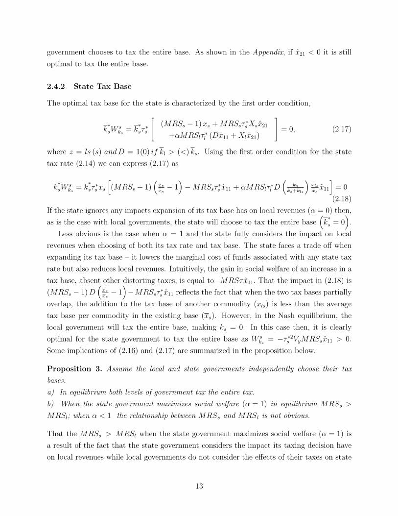
That the MRSs > MRSl when the state government maximizes social welfare (α = 1) is

a result of the fact that the state government considers the impact its taxing decision have

on local revenues while local governments do not consider the effects of their taxes on state

13

revenues. The relationship between MRSsand MRSl can be obtained by subtracting the

first order condition for the local tax rate, (2.11), from that of the state (2.14) to obtain

MRSs =

[1 + (1− α) τ ∗l (x̂11 + x̂21)

1 + τ ∗s (x̂11 + x̂21)

]MRSl. (2.19)

3 Optimal Tax Base Division and Co-occupancy

As shown in the preceding section, both levels of government will tax the entire tax base

if given the option. Changes in the local governments’ tax bases as well as their tax rates

will generate fiscal externalities. Here I address the question of what is the social-welfare

maximizing division of the tax base between the two levels of government. I first address the

question of how the tax base should be divided if there is no co-occupancy. After deriving

the optimal division of the tax base, the question of whether the state and local governments

should share tax bases, that is, whether there should be any co-occupancy, is then addressed.

If the state government fully considers the impacts of its tax policy on local revenues

(α = 1), if it were also have the authority to determine the extent of both its and the local

governments tax bases, the choices would be welfare-maximizing. However, if α < 1, the

state government does not fully consider the impacts of its tax policy on local revenues.

Then, in this case, if the state government were to determine the tax bases for both levels

of government it would not choose the welfare-maximizing division. As I wish to investi-

gate the welfare-maximizing division of the tax base in the case of α < 1 rather than the

state government determining the tax base division, a third-party (federal government or

“planner”) chooses the tax bases to maximize social welfare.

In addition to having a third party choose the optimal division of the tax base, the timing

of the division of the tax base, relative to the setting of the state and local tax rates, also

needs to be determined. My focus will be on a Nash equilibrium in which the state and local

governments choose their tax rates at the same time as the planner chooses the division of

the tax base. In Section 3.3 I discuss a two-stage game in which the federal government

chooses the division of the tax base in the first stage of the game and the state and local

governments simultaneously set their tax rates in the second stage.

3.1 The Optimal Division of the Tax Base

The optimal division of the tax base in the absence of co-occupancy solves

Max

klW[τl, τs, kl

]=

ˆ 1

0

V (k) dk + U s(gs(τl, τs, kl

))+ αU l

(gl(τl, τs, kl

))(3.1)

14

where, given no co-occupancy, kl = kl and ks = 1− kl. Then the optimal division of the tax

base, k∗l , that satisfies the first order condition for (3.1) can be expressed as

τ ∗l

[(−1 +MRSl (1 + τ ∗l klx̂21))xl

(a)+

MRSsτ∗s ksxsx̂21

(b)

]=

τ ∗s

[(−1 +MRSs (1 + τ ∗s ksx̂21))xs

(c)+

MRSlτ∗l klxlx̂21

(d)

] (3.2)

where, again, τ ∗l and τ ∗s are the equilibrium tax rates. Derivation of (3.2) and other equations

as well as proofs of propositions in this section are found in Appendix A.3. The expansion

of the local tax base and contraction of the state tax base directly increases local revenue

by τlxl and indirectly by affecting the price of x(kl), now taxed at a rate of τ l rather than

τ s. As well, the tax has a direct impact through its impact on the price of x(kl). These

impacts of found in term (a) of (3.2). Term (b) is the impact of adding x(kl)

to the local

tax base on state tax revenues. Then the optimal division of the tax base must be such that

the impact on utility of the expansion of the local tax base is exactly offset by the impact

of the equal reduction of the state tax base, terms (c) and (d) of (3.2). Rearranging terms

in (3.2) yields

(MRSl − 1) τ ∗l xl − (MRSs − 1) τ ∗s xs+

(a)

(τ ∗l − τ ∗s ) (MRSlτ∗l klxl +MRSsτ

∗s ksxs) x̂21 = 0.

(b)

(3.3)

Examination of equation (3.3) provides for additional characterization of the optimal division

of the tax base. From (3.3) we can see that if commodities are substitutes (x̂21 > 0) the sign

of term (b) is the sign of τ l− τ s. Then if, for example, τ l > τ s it must be the case that term

(a) is negative, requiring MRSl < MRSs. If τ l(.5) > (<)τ s(.5) then Wkl

∣∣kl=.5

> (<) 0 and

the optimal division of the tax base must be k∗l > (<).5. With x̂21 > 0 and k

∗l > (<).5 (3.3)

can only be satisfied when the optimal tax rates are τ ∗l > (<)τ ∗s .

When commodities are complements or α 6= 0, the relationship between the relative tax

rates and the relative MRS is indeterminate – with τ l > τ s it is possible to have MRSl <

MRSs or MRSl > MRSs and satisfy (3.3). This being the case, it is possible for (3.3)

to be satisfied with no obvious relationship between the equilibrium tax rates (τ ∗l , τ∗s), the

associate MRS, and the relative tax rates when the base is evenly split.

Proposition 4. In the absence of co-occupancy, the optimal division(k∗l

)of the tax base

can be characterized by the following:

a) If α = 0 and i) τ l (.5) > (<)τ s (.5) then k∗l > (<).5; ii) x̂21 > 0 and τ l (.5) > (<)τ s (.5)

15

then τ l

(k∗l

)> (<)τ s

(k∗l

)and MRSl

(k∗l

)< (>)MRSs

(k∗l

).b) If α = 1 and i) x̂21 > 0

and τ l (.5) ≥ τ s (.5) then k∗l > .5 and ; ii) x̂21 < 0 and τ l (.5) ≤ τ s (.5) then k

∗l < .5; iii)

x̂21 > 0 then τ l

(k∗l

)< τ s

(k∗l

); and iv) x̂21 < 0 then τ l

(k∗l

)> τ s

(k∗l

).

c) At k∗l , MRSlτ l

(k∗l

)6= MRSsτ s

(k∗s

).

d) At k∗l : i) if x̂21 = 0, a (marginal) change in either the local or state tax rate has no impact

on social welfare; ii) if x̂21 > (<) 0 and α = 0, an increase (decrease) in the local or state

tax rate will increase social welfare; iii) if x̂21 > (<) 0, and α = 1 an increase (decrease) in

the local tax rate will increase social welfare while an increase in the state tax rate will have

no impact on social welfare.

Proof of the proposition is found in Appendix A.3.2. Part c) of the proposition, MRSlτ l

(k∗l

)6=

MRSsτ s

(k∗s

), is important when considering whether co-occupancy is optimal. Part d)

provides relationships between the division of the tax base and the fiscal externality from

increases in the tax rates. As suggested by the proposition, the division of the tax base will

not eliminate the fiscal externalities associated with the two tax rates when commodities

have non-zero cross-price elasticities. This can easily be seen by differentiating the social

welfare function with respect to the tax rate of a single locality,

Wτl =1

nMRSsτs

(1− k∗l

)k∗l x̂21 (3.4)

In the case of gross substitutes, it may change the fiscal externality from being negative

with co-occupancy to being positive with no co-occupancy. This, in turn, means that taxes

also change from being “too” high to being “too” low, that is, below the welfare maximizing

rates.

3.2 Optimal Co-Occupancy of Tax Bases

That the tax rates and marginal rates of substitutions for the public services are not equal for

the two levels of government and tax rate increases or decreases can enhance social welfare

suggests at least the possibility that co-occupancy may be desirable. Below I consider the

possibility of co-occupancy and under what conditions it may be socially optimal.

The problem facing the planner is

Maximize

kl, ksW(kl, ks, τs, τl

)=

ˆ 1

0

V (q(k)dk + U s(gs(kl, ks, τs, τl

))+ U l

(gl(kl, ks, τs, τl

))(3.5)

16

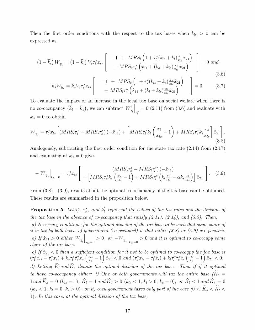
Then the first order conditions with the respect to the tax bases when kls > 0 can be

expressed as

(1− kl

)W

kl=(1− kl

)Vyτ

∗l xls

−1 + MRSl

(1 + τ ∗l (kls + kl)

xlxlsx̂21

)+ MRSsτ

∗s

(x̂11 + (ks + kls)

xsxlsx̂21

) = 0 and

(3.6)

ksWks= ksVyτ

∗s xls

−1 + MRSs

(1 + τ ∗s (kls + ks)

xsxlsx̂21

)+ MRSlτ

∗l

(x̂11 + (kl + kls)

xlxlsx̂21

) = 0. (3.7)

To evaluate the impact of an increase in the local tax base on social welfare when there is

no co-occupancy(kl = ks

), we can subtract W l

τl

∣∣∣τ∗l

= 0 (2.11) from (3.6) and evaluate with

kls = 0 to obtain

Wkl

= τ ∗l xls

[(MRSlτ

∗l −MRSsτ

∗s ) (−x̂11) +

[MRSlτ

∗l kl

(xlxls− 1

)+MRSsτ

∗s ks

xsxls

]x̂21

].

(3.8)

Analogously, subtracting the first order condition for the state tax rate (2.14) from (2.17)

and evaluating at kls = 0 gives

−Wks

∣∣∣kls=0

= τ ∗s xls

[(MRSsτ

∗s −MRSlτ

∗l ) (−x̂11)

+[MRSsτ

∗s ks

(xsxls− 1)

+MRSlτ∗l

(kl

xlxls− αks xlxls

)]x̂21

]. (3.9)

From (3.8) - (3.9), results about the optimal co-occupancy of the tax base can be obtained.

These results are summarized in the proposition below.

Proposition 5. Let τ ∗l , τ∗s , and k

∗l represent the values of the tax rates and the division of

the tax base in the absence of co-occupancy that satisfy (2.11), (2.14), and (3.3). Then:

a) Necessary conditions for the optimal division of the tax base to be such that some share ofit is tax by both levels of government (co-occupied) is that either (3.8) or (3.9) are positive.

b) If x̂21 > 0 either Wkl

∣∣∣kls=0

> 0 or −Wks

∣∣∣kls=0

> 0 and it is optimal to co-occupy some

share of the tax base.

c) If x̂21 < 0 then a sufficient condition for it not to be optimal to co-occupy the tax base is(τ ∗l xls − τ ∗s xs) + ksτ

∗l τ̃

∗s xs

(xlsxs− 1)x̂21 < 0 and (τ ∗s xls − τ ∗l xl) + klτ̃

∗l τ

∗s xl

(xlsxl− 1)x̂21 < 0.

d) Letting K̃l and K̃s denote the optimal division of the tax base. Then if if it optimal

to have co-occupancy either: i) One or both governments will tax the entire base (K̃l =

1 and K̃s = 0 (kls = 1), K̃l = 1 and K̃s > 0 (kls < 1, kl > 0, ks = 0), or K̃l < 1 and K̃s = 0

(kls < 1, kl = 0, ks > 0) . or ii) each government taxes only part of the base (0 < K̃s < K̃l <

1). In this case, at the optimal division of the tax base,

17

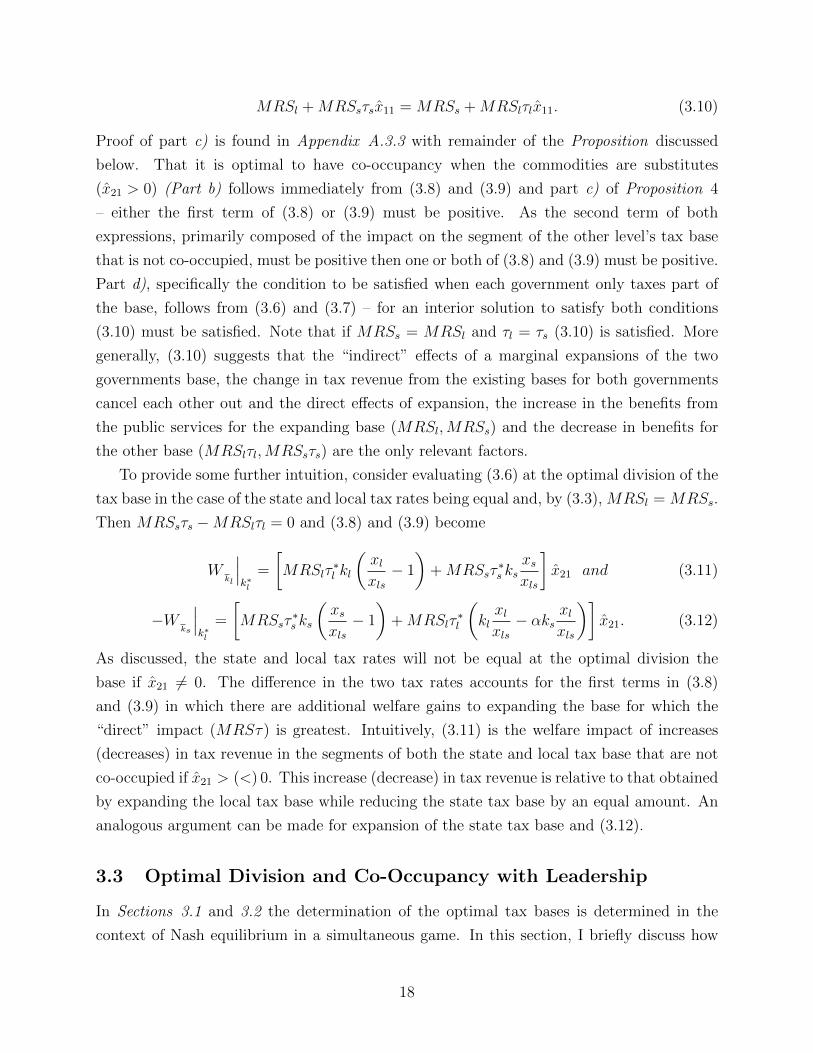
MRSl +MRSsτsx̂11 = MRSs +MRSlτlx̂11. (3.10)

Proof of part c) is found in Appendix A.3.3 with remainder of the Proposition discussed

below. That it is optimal to have co-occupancy when the commodities are substitutes

(x̂21 > 0) (Part b) follows immediately from (3.8) and (3.9) and part c) of Proposition 4

– either the first term of (3.8) or (3.9) must be positive. As the second term of both

expressions, primarily composed of the impact on the segment of the other level’s tax base

that is not co-occupied, must be positive then one or both of (3.8) and (3.9) must be positive.

Part d), specifically the condition to be satisfied when each government only taxes part of

the base, follows from (3.6) and (3.7) – for an interior solution to satisfy both conditions

(3.10) must be satisfied. Note that if MRSs = MRSl and τl = τs (3.10) is satisfied. More

generally, (3.10) suggests that the “indirect” effects of a marginal expansions of the two

governments base, the change in tax revenue from the existing bases for both governments

cancel each other out and the direct effects of expansion, the increase in the benefits from

the public services for the expanding base (MRSl,MRSs) and the decrease in benefits for

the other base (MRSlτl,MRSsτs) are the only relevant factors.

To provide some further intuition, consider evaluating (3.6) at the optimal division of the

tax base in the case of the state and local tax rates being equal and, by (3.3), MRSl = MRSs.

Then MRSsτs −MRSlτl = 0 and (3.8) and (3.9) become

Wkl

∣∣∣k∗l

=

[MRSlτ

∗l kl

(xlxls− 1

)+MRSsτ

∗s ks

xsxls

]x̂21 and (3.11)

−Wks

∣∣∣k∗l

=

[MRSsτ

∗s ks

(xsxls− 1

)+MRSlτ

∗l

(klxlxls− αks

xlxls

)]x̂21. (3.12)

As discussed, the state and local tax rates will not be equal at the optimal division the

base if x̂21 6= 0. The difference in the two tax rates accounts for the first terms in (3.8)

and (3.9) in which there are additional welfare gains to expanding the base for which the

“direct” impact (MRSτ) is greatest. Intuitively, (3.11) is the welfare impact of increases

(decreases) in tax revenue in the segments of both the state and local tax base that are not

co-occupied if x̂21 > (<) 0. This increase (decrease) in tax revenue is relative to that obtained

by expanding the local tax base while reducing the state tax base by an equal amount. An

analogous argument can be made for expansion of the state tax base and (3.12).

3.3 Optimal Division and Co-Occupancy with Leadership

In Sections 3.1 and 3.2 the determination of the optimal tax bases is determined in the

context of Nash equilibrium in a simultaneous game. In this section, I briefly discuss how

18

the results in these sections might change if rather than having simultaneous determination

of both the tax bases and tax rates, they are determined in a two-stage game and show that

the results are qualitatively unchanged.

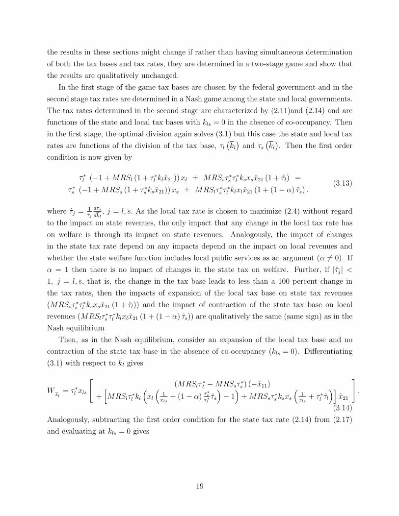
In the first stage of the game tax bases are chosen by the federal government and in the

second stage tax rates are determined in a Nash game among the state and local governments.

The tax rates determined in the second stage are characterized by (2.11)and (2.14) and are

functions of the state and local tax bases with kls = 0 in the absence of co-occupancy. Then

in the first stage, the optimal division again solves (3.1) but this case the state and local tax

rates are functions of the division of the tax base, τl(kl)

and τs(kl). Then the first order

condition is now given by

τ ∗l (−1 +MRSl (1 + τ ∗l klx̂21))xl + MRSsτ∗s τ

∗l ksxsx̂21 (1 + τ̂l) =

τ ∗s (−1 +MRSs (1 + τ ∗s ksx̂21))xs + MRSlτ∗s τ

∗l klxlx̂21 (1 + (1− α) τ̂s) .

(3.13)

where τ̂j = 1τj

dτjdkl, j = l, s. As the local tax rate is chosen to maximize (2.4) without regard

to the impact on state revenues, the only impact that any change in the local tax rate has

on welfare is through its impact on state revenues. Analogously, the impact of changes

in the state tax rate depend on any impacts depend on the impact on local revenues and

whether the state welfare function includes local public services as an argument (α 6= 0). If

α = 1 then there is no impact of changes in the state tax on welfare. Further, if |τ̂j| <1, j = l, s, that is, the change in the tax base leads to less than a 100 percent change in

the tax rates, then the impacts of expansion of the local tax base on state tax revenues

(MRSsτ∗s τ

∗l ksxsx̂21 (1 + τ̂l)) and the impact of contraction of the state tax base on local

revenues (MRSlτ∗s τ

∗l klxlx̂21 (1 + (1− α) τ̂s)) are qualitatively the same (same sign) as in the

Nash equilibrium.

Then, as in the Nash equilibrium, consider an expansion of the local tax base and no

contraction of the state tax base in the absence of co-occupancy (kls = 0). Differentiating

(3.1) with respect to kl gives

Wkl

= τ ∗l xls

[(MRSlτ

∗l −MRSsτ

∗s ) (−x̂11)

+[MRSlτ

∗l kl

(xl

(1xls

+ (1− α) τ∗sτ∗lτ̂s

)− 1)

+MRSsτ∗s ksxs

(1xls

+ τ ∗l τ̂l

)]x̂21

].

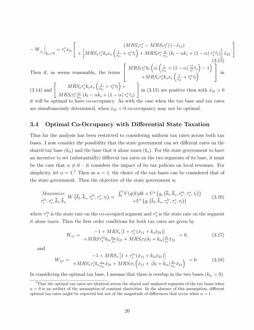
(3.14)

Analogously, subtracting the first order condition for the state tax rate (2.14) from (2.17)

and evaluating at kls = 0 gives

19

−Wks

∣∣∣kls=0

= τ ∗s xls

[(MRSsτ

∗s −MRSlτ

∗l ) (−x̂11)

+[MRSsτ

∗s ksxs

(1xls

+ τ ∗l τ̂l

)+MRSlτ

∗lxlxls

(kl − αks + (1− α) τ ∗s τ̂s)]x̂21

].

(3.15)

Then if, as seems reasonable, the terms

MRSlτ∗l kl

(xl

(1xls

+ (1− α) τ∗sτ∗lτ̂s

)− 1)

+MRSsτ∗s ksxs

(1xls

+ τ ∗l τ̂l

) in

(3.14) and

[MRSsτ

∗s ksxs

(1xls

+ τ ∗l τ̂l

)+

MRSlτ∗lxlxls

(kl − αks + (1− α) τ ∗s τ̂s)

]in (3.15) are positive then with x̂21 > 0

it will be optimal to have co-occupancy. As with the case when the tax base and tax rates

are simultaneously determined, when x̂21 < 0 co-occupancy may not be optimal.

3.4 Optimal Co-Occupancy with Differential State Taxation

Thus far the analysis has been restricted to considering uniform tax rates across both tax

bases. I now consider the possibility that the state government can set different rates on the

shared tax base (kls) and the base that it alone taxes (ks). For the state government to have

an incentive to set (substantially) different tax rates on the two segments of its base, it must

be the case that α 6= 0 – it considers the impact of its tax policies on local revenues. For

simplicity, let α = 1.7 Then as α = 1, the choice of the tax bases can be considered that of

the state government. Then the objective of the state government is

Maximize

τ lss , τss , kl, ks

W(kl, ks, τ

lss , τ

ss , τl

)=

´ 10V (q(k)dk + U s

(gs(kl, ks, τ

lss , τ

ss , τl

))+U l

(gl(kl, ks, τ

lss , τ

ss , τl

)) (3.16)

where τ lss is the state rate on the co-occupied segment and τ ss is the state rate on the segment

it alone taxes. Then the first order conditions for both tax rates are given by

Wτss =−1 +MRSs [1 + τ ss (x̂11 + ksx̂21)]

+MRSτ lss klsxlsxsx̂21 +MRSlτl(kl + kls)

xlxsx̄21

= 0, (3.17)

and

Wτ lss=

−1 +MRSs[1 + τ lss (x̂11 + klsx̂21)

]+MRSsτ

ss ks

xsxlsx̂21 +MRSlτl

(x̂11 + (kl + kls)

xlxlsx̂21

) = 0. (3.18)

In considering the optimal tax base, I assume that there is overlap in the two bases (kls > 0).

7That the optimal tax rates are identical across the shared and unshared segments of the tax bases whenα = 0 is an artifact of the assumption of constant elasticities. In the absence of this assumption, differentoptimal tax rates might be expected but not of the magnitude of differences that occur when α = 1.

20

Then an increase in kl means a reduction in the base only taxed by the state (ks) and a

decrease in ks means a reduction in the base only taxed by the localities (kl). Then the

optimal tax bases are determined by

(1− kl

)W

kl=(1− kl

) [ [(MRSl − 1) τl + (MRSs − 1) τ lss

]xls − (MRSs − 1) τ ssxs+[

MRSlτl (kl + kls)xl +MRSs(τ lss klsxls + τ ss ksxs

)]x̂21(τl + τ lss − τ ss

) ] = 0,

(3.19)

and

−ksW ks=(1− ks

) [ [(MRSl − 1) τl + (MRSs − 1) τ lss]xls − (MRSl − 1) τlxl+[

MRSlτl (kl + kls)xl +MRSs(τ lss klsxls + τ ss ksxs

)]x̂21τ

lss

]= 0.

(3.20)

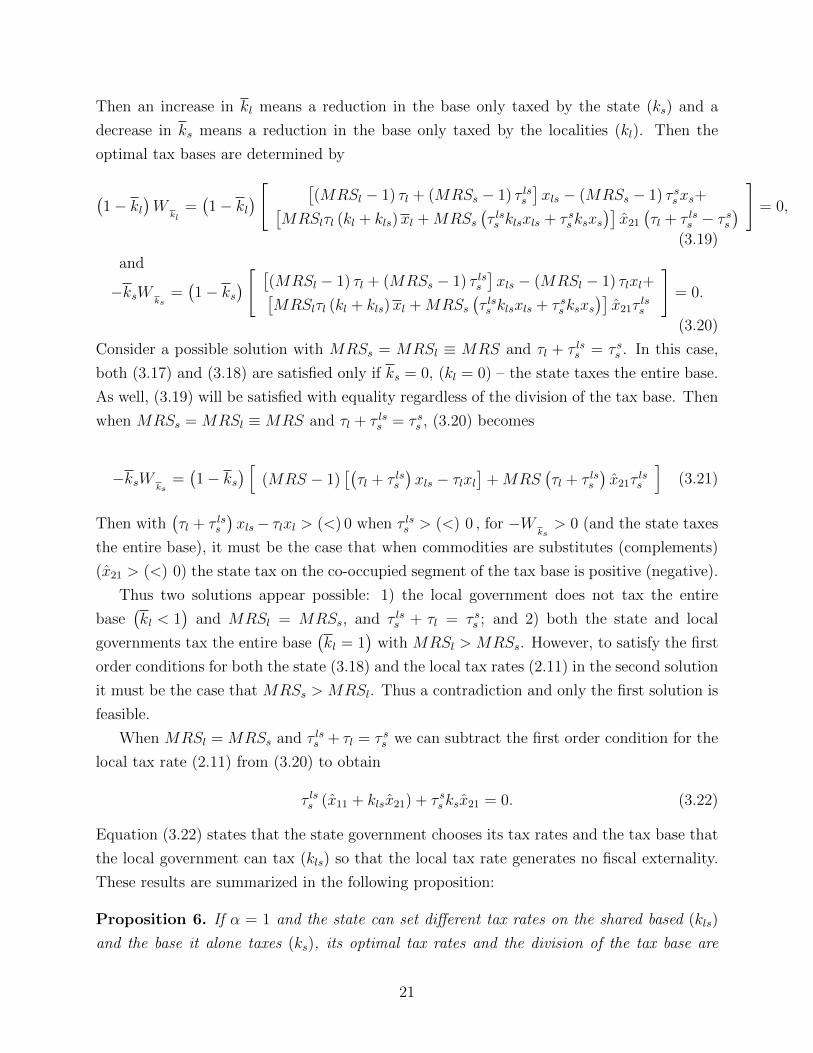
Consider a possible solution with MRSs = MRSl ≡ MRS and τl + τ lss = τ ss . In this case,

both (3.17) and (3.18) are satisfied only if ks = 0, (kl = 0) – the state taxes the entire base.

As well, (3.19) will be satisfied with equality regardless of the division of the tax base. Then

when MRSs = MRSl ≡MRS and τl + τ lss = τ ss , (3.20) becomes

−ksW ks=(1− ks

) [(MRS − 1)

[(τl + τ lss

)xls − τlxl

]+MRS

(τl + τ lss

)x̂21τ

lss

](3.21)

Then with(τl + τ lss

)xls− τlxl > (<) 0 when τ lss > (<) 0 , for −W

ks> 0 (and the state taxes

the entire base), it must be the case that when commodities are substitutes (complements)

(x̂21 > (<) 0) the state tax on the co-occupied segment of the tax base is positive (negative).

Thus two solutions appear possible: 1) the local government does not tax the entire

base(kl < 1

)and MRSl = MRSs, and τ lss + τl = τ ss ; and 2) both the state and local

governments tax the entire base(kl = 1

)with MRSl > MRSs. However, to satisfy the first

order conditions for both the state (3.18) and the local tax rates (2.11) in the second solution

it must be the case that MRSs > MRSl. Thus a contradiction and only the first solution is

feasible.

When MRSl = MRSs and τ lss + τl = τ ss we can subtract the first order condition for the

local tax rate (2.11) from (3.20) to obtain

τ lss (x̂11 + klsx̂21) + τ ss ksx̂21 = 0. (3.22)

Equation (3.22) states that the state government chooses its tax rates and the tax base that

the local government can tax (kls) so that the local tax rate generates no fiscal externality.

These results are summarized in the following proposition:

Proposition 6. If α = 1 and the state can set different tax rates on the shared based (kls)

and the base it alone taxes (ks), its optimal tax rates and the division of the tax base are

21

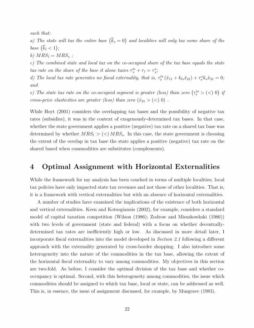
such that:

a) The state will tax the entire base(ks = 0

)and localities will only tax some share of the

base(kl < 1

);

b) MRSl = MRSs ;

c) The combined state and local tax on the co-occupied share of the tax base equals the state

tax rate on the share of the base it alone taxes τ lss + τ l = τ ss;

d) The local tax rate generates no fiscal externality, that is, τ lss (x̂11 + klsx̂21) + τ ss ksx̂21 = 0;

and

e) The state tax rate on the co-occupied segment is greater (less) than zero(τ lss > (<) 0

)if

cross-price elasticities are greater (less) than zero (x̂21 > (<) 0) .

While Hoyt (2001) considers the overlapping tax bases and the possibility of negative tax

rates (subsidies), it was in the context of exogenously-determined tax bases. In that case,

whether the state government applies a positive (negative) tax rate on a shared tax base was

determined by whether MRSl > (<)MRSs. In this case, the state government is choosing

the extent of the overlap in tax base the state applies a positive (negative) tax rate on the

shared based when commodities are substitutes (complements).

4 Optimal Assignment with Horizontal Externalities

While the framework for my analysis has been couched in terms of multiple localities, local

tax policies have only impacted state tax revenues and not those of other localities. That is,

it is a framework with vertical externalities but with an absence of horizontal externalities.

A number of studies have examined the implications of the existence of both horizontal

and vertical externalities. Keen and Kotsogiannis (2002), for example, considers a standard

model of capital taxation competition (Wilson (1986); Zodrow and Mieszkowkski (1986))

with two levels of government (state and federal) with a focus on whether decentrally-

determined tax rates are inefficiently high or low. As discussed in more detail later, I

incorporate fiscal externalities into the model developed in Section 2.1 following a different

approach with the externality generated by cross-border shopping. I also introduce some

heterogeneity into the nature of the commodities in the tax base, allowing the extent of

the horizontal fiscal externality to vary among commodities. My objectives in this section

are two-fold. As before, I consider the optimal division of the tax base and whether co-

occupancy is optimal. Second, with this heterogeneity among commodities, the issue which

commodities should be assigned to which tax base, local or state, can be addressed as well.

This is, in essence, the issue of assignment discussed, for example, by Musgrave (1983).

22

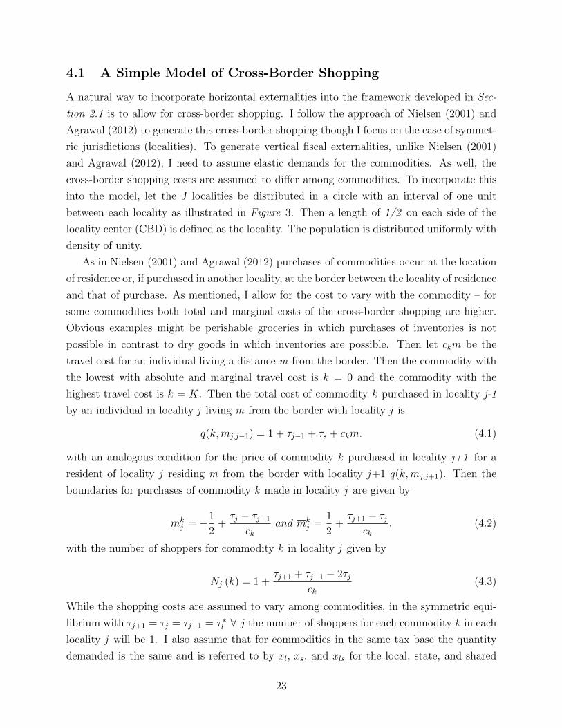
4.1 A Simple Model of Cross-Border Shopping

A natural way to incorporate horizontal externalities into the framework developed in Sec-

tion 2.1 is to allow for cross-border shopping. I follow the approach of Nielsen (2001) and

Agrawal (2012) to generate this cross-border shopping though I focus on the case of symmet-

ric jurisdictions (localities). To generate vertical fiscal externalities, unlike Nielsen (2001)

and Agrawal (2012), I need to assume elastic demands for the commodities. As well, the

cross-border shopping costs are assumed to differ among commodities. To incorporate this

into the model, let the J localities be distributed in a circle with an interval of one unit

between each locality as illustrated in Figure 3. Then a length of 1/2 on each side of the

locality center (CBD) is defined as the locality. The population is distributed uniformly with

density of unity.

As in Nielsen (2001) and Agrawal (2012) purchases of commodities occur at the location

of residence or, if purchased in another locality, at the border between the locality of residence

and that of purchase. As mentioned, I allow for the cost to vary with the commodity – for

some commodities both total and marginal costs of the cross-border shopping are higher.

Obvious examples might be perishable groceries in which purchases of inventories is not

possible in contrast to dry goods in which inventories are possible. Then let ckm be the

travel cost for an individual living a distance m from the border. Then the commodity with

the lowest with absolute and marginal travel cost is k = 0 and the commodity with the

highest travel cost is k = K. Then the total cost of commodity k purchased in locality j-1

by an individual in locality j living m from the border with locality j is

q(k,mj,j−1) = 1 + τj−1 + τs + ckm. (4.1)

with an analogous condition for the price of commodity k purchased in locality j+1 for a

resident of locality j residing m from the border with locality j +1 q(k,mj,j+1). Then the

boundaries for purchases of commodity k made in locality j are given by

mkj = −1

2+τj − τj−1

ckand mk

j =1

2+τj+1 − τj

ck. (4.2)

with the number of shoppers for commodity k in locality j given by

Nj (k) = 1 +τj+1 + τj−1 − 2τj

ck(4.3)

While the shopping costs are assumed to vary among commodities, in the symmetric equi-

librium with τj+1 = τj = τj−1 = τ ∗l ∀ j the number of shoppers for each commodity k in each

locality j will be 1. I also assume that for commodities in the same tax base the quantity

demanded is the same and is referred to by xl, xs, and xls for the local, state, and shared

23

bases as before.

The expression for the local government budget is complicated. It depends on the tax

rates in the two adjacent localities and, unlike, the framework developed in Sections 2 and 3

not simply the lengths of the tax intervals (number of commodities taxed) as the commodities

differ in responses to taxes in other localities. An expression for it can be found in Appendix

A.4. As our interest is in analyzing equilibrium policies, I consider the impact of a local

tax increase when all localities set the same tax rates and, therefore, mkj = −1

2and mk

j = 12

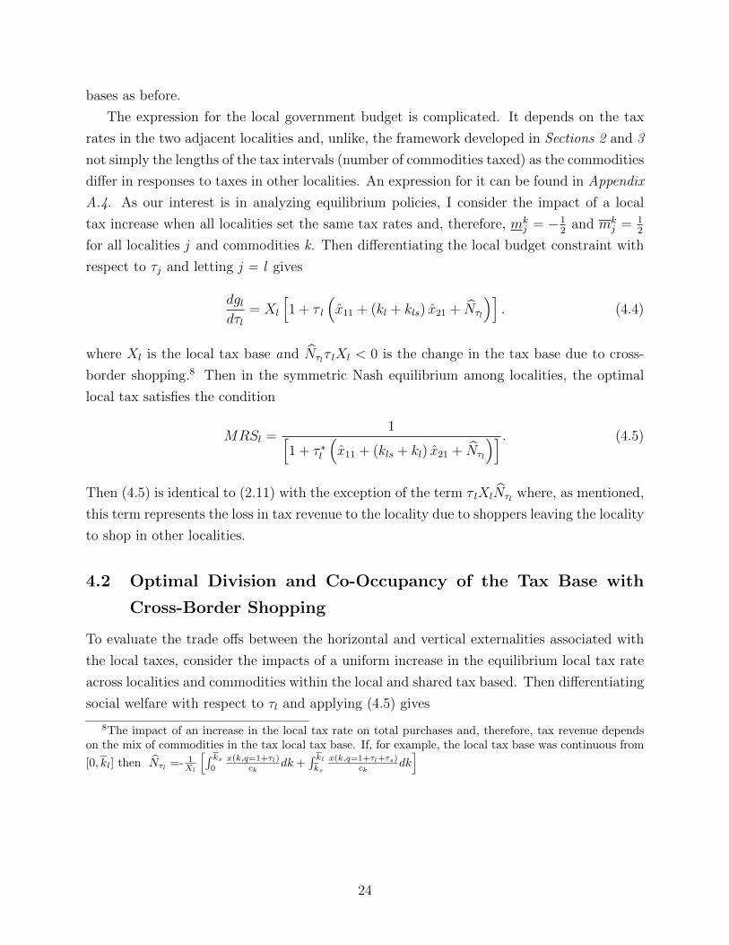
for all localities j and commodities k. Then differentiating the local budget constraint with

respect to τj and letting j = l gives

dgldτl

= Xl

[1 + τ l

(x̂11 + (kl + kls) x̂21 + N̂τl

)]. (4.4)

where Xl is the local tax base and N̂τlτ lXl < 0 is the change in the tax base due to cross-

border shopping.8 Then in the symmetric Nash equilibrium among localities, the optimal

local tax satisfies the condition

MRSl =1[

1 + τ ∗l

(x̂11 + (kls + kl) x̂21 + N̂τl

)] . (4.5)

Then (4.5) is identical to (2.11) with the exception of the term τ lXlN̂τl where, as mentioned,

this term represents the loss in tax revenue to the locality due to shoppers leaving the locality

to shop in other localities.

4.2 Optimal Division and Co-Occupancy of the Tax Base with

Cross-Border Shopping

To evaluate the trade offs between the horizontal and vertical externalities associated with

the local taxes, consider the impacts of a uniform increase in the equilibrium local tax rate

across localities and commodities within the local and shared tax based. Then differentiating

social welfare with respect to τl and applying (4.5) gives

8The impact of an increase in the local tax rate on total purchases and, therefore, tax revenue dependson the mix of commodities in the tax local tax base. If, for example, the local tax base was continuous from

[0, kl] then N̂τl =- 1Xl

[´ ks0

x(k,q=1+τl)ck

dk +´ klks

x(k,q=1+τl+τs)ck

dk]

24

dW

dτl= VyXl

−MRSlτlXlN̂τl

(a)+

MRSsτs

(kls

(kl+kls)xlsxlx̂11 + (ks + kls)

xsxlx̂21

)(b)

+MRSlτl

(kls

(kl+kls)xlsxlx̂11 + (ks + kls) x̂21

)dτsdτl

(c)

. (4.6)

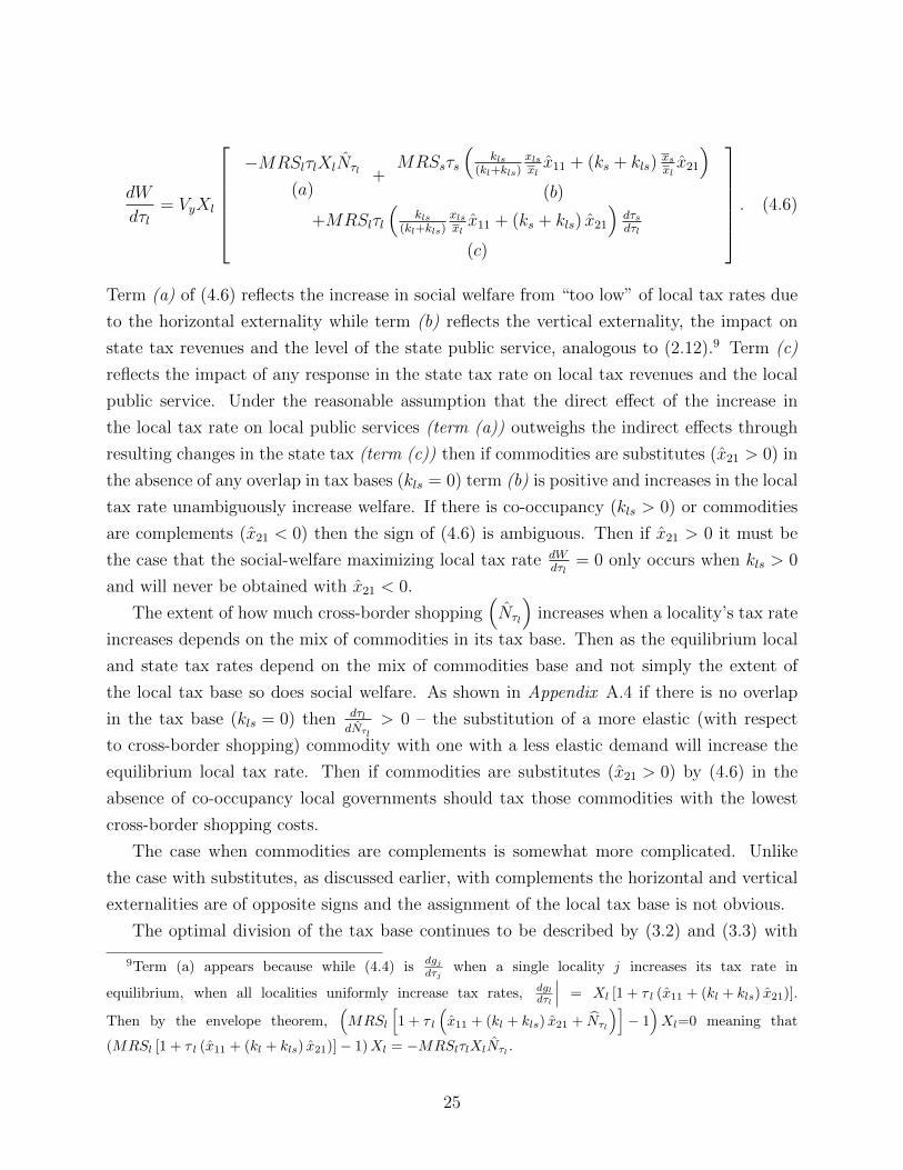
Term (a) of (4.6) reflects the increase in social welfare from “too low” of local tax rates due

to the horizontal externality while term (b) reflects the vertical externality, the impact on

state tax revenues and the level of the state public service, analogous to (2.12).9 Term (c)

reflects the impact of any response in the state tax rate on local tax revenues and the local

public service. Under the reasonable assumption that the direct effect of the increase in

the local tax rate on local public services (term (a)) outweighs the indirect effects through

resulting changes in the state tax (term (c)) then if commodities are substitutes (x̂21 > 0) in

the absence of any overlap in tax bases (kls = 0) term (b) is positive and increases in the local

tax rate unambiguously increase welfare. If there is co-occupancy (kls > 0) or commodities

are complements (x̂21 < 0) then the sign of (4.6) is ambiguous. Then if x̂21 > 0 it must be

the case that the social-welfare maximizing local tax rate dWdτl

= 0 only occurs when kls > 0

and will never be obtained with x̂21 < 0.

The extent of how much cross-border shopping(N̂τl

)increases when a locality’s tax rate

increases depends on the mix of commodities in its tax base. Then as the equilibrium local

and state tax rates depend on the mix of commodities base and not simply the extent of

the local tax base so does social welfare. As shown in Appendix A.4 if there is no overlap

in the tax base (kls = 0) then dτldN̂τl

> 0 – the substitution of a more elastic (with respect

to cross-border shopping) commodity with one with a less elastic demand will increase the

equilibrium local tax rate. Then if commodities are substitutes (x̂21 > 0) by (4.6) in the

absence of co-occupancy local governments should tax those commodities with the lowest

cross-border shopping costs.

The case when commodities are complements is somewhat more complicated. Unlike

the case with substitutes, as discussed earlier, with complements the horizontal and vertical

externalities are of opposite signs and the assignment of the local tax base is not obvious.

The optimal division of the tax base continues to be described by (3.2) and (3.3) with

9Term (a) appears because while (4.4) isdgjdτj

when a single locality j increases its tax rate in

equilibrium, when all localities uniformly increase tax rates, dgldτl

∣∣∣ = Xl [1 + τ l (x̂11 + (kl + kls) x̂21)].

Then by the envelope theorem,(MRSl

[1 + τ l

(x̂11 + (kl + kls) x̂21 + N̂τl

)]− 1)Xl=0 meaning that

(MRSl [1 + τ l (x̂11 + (kl + kls) x̂21)]− 1)Xl = −MRSlτlXlN̂τl .

25

modifications to allow for the heterogeneity in the local tax base arising from cross-border

shopping. Adding a commodity to the local tax base and removing it from the state tax

base means that differences in local tax rates will induce cross-border shopping. However,

as in equilibrium all local governments will have the same tax rates, there will be no impact

on the tax base due to cross-border shopping.

However, when evaluating the optimal division of the tax base at the optimally-chosen

tax rates for the local governments (4.5) and the state (2.14) government with cross-border

shopping, the characterization of the optimal division of the tax base is no longer analogous.

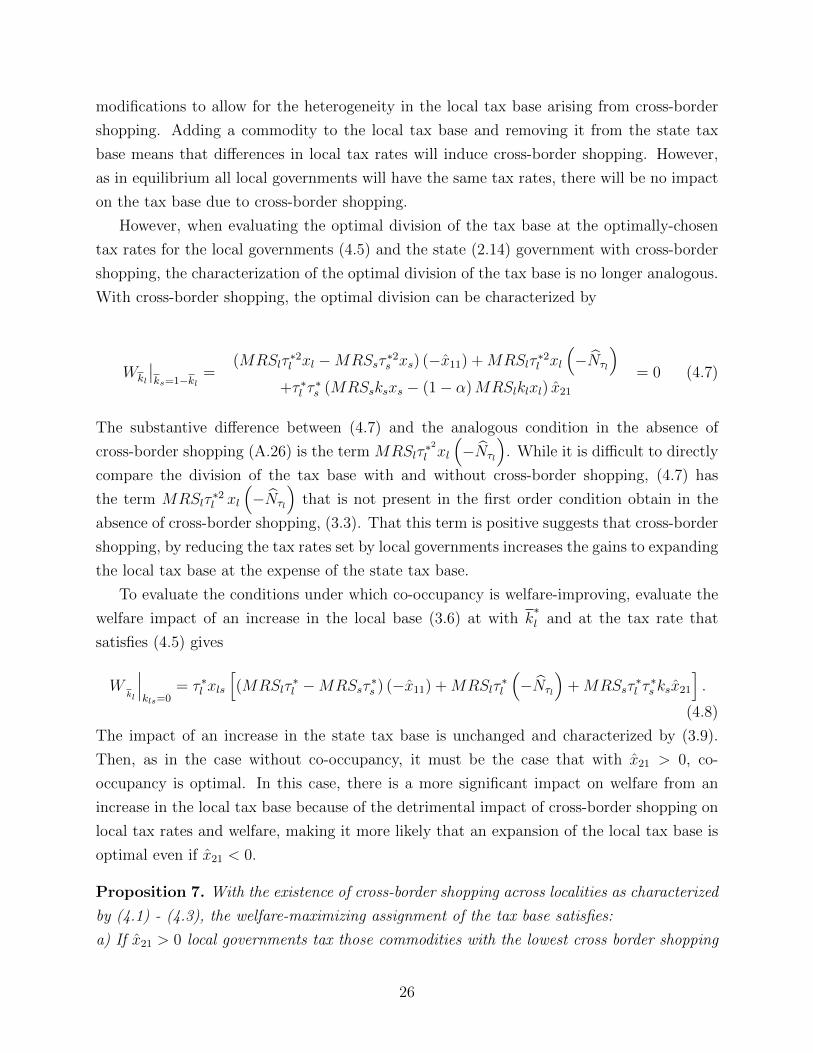
With cross-border shopping, the optimal division can be characterized by

Wkl

∣∣ks=1−kl

=(MRSlτ

∗2l xl −MRSsτ

∗2s xs) (−x̂11) +MRSlτ

∗2l xl

(−N̂τl

)+τ ∗l τ

∗s (MRSsksxs − (1− α)MRSlklxl) x̂21

= 0 (4.7)

The substantive difference between (4.7) and the analogous condition in the absence of

cross-border shopping (A.26) is the term MRSlτ∗2l xl

(−N̂τl

). While it is difficult to directly

compare the division of the tax base with and without cross-border shopping, (4.7) has

the term MRSlτ∗2l xl

(−N̂τl

)that is not present in the first order condition obtain in the

absence of cross-border shopping, (3.3). That this term is positive suggests that cross-border

shopping, by reducing the tax rates set by local governments increases the gains to expanding

the local tax base at the expense of the state tax base.

To evaluate the conditions under which co-occupancy is welfare-improving, evaluate the

welfare impact of an increase in the local base (3.6) at with k∗l and at the tax rate that

satisfies (4.5) gives

Wkl

∣∣∣kls=0

= τ ∗l xls

[(MRSlτ

∗l −MRSsτ

∗s ) (−x̂11) +MRSlτ

∗l

(−N̂τl

)+MRSsτ

∗l τ

∗s ksx̂21

].

(4.8)

The impact of an increase in the state tax base is unchanged and characterized by (3.9).

Then, as in the case without co-occupancy, it must be the case that with x̂21 > 0, co-

occupancy is optimal. In this case, there is a more significant impact on welfare from an

increase in the local tax base because of the detrimental impact of cross-border shopping on

local tax rates and welfare, making it more likely that an expansion of the local tax base is

optimal even if x̂21 < 0.

Proposition 7. With the existence of cross-border shopping across localities as characterized

by (4.1) - (4.3), the welfare-maximizing assignment of the tax base satisfies:

a) If x̂21 > 0 local governments tax those commodities with the lowest cross border shopping

26

costs (ck);

b) The optimal division of the tax bases satisfies (4.7) in the absence of co-occupancy;

c) If (4.8) or (3.9) are positive then it is optimal to have co-occupancy; if x̂21 > 0 then either

(4.8) or (3.9) is positive and it is optimal to have co-occupancy.

5 Concluding Comments

The conventional wisdom suggests that separate tax bases for different levels of government is

preferred to reduce the extent of vertical externalities and the over-provision of public services

associated with the vertical externality. However, most previous studies have not considered

the impacts of tax rates across revenues sources, that is, across tax bases. Specifically,

how changes in tax rates in one base may influence revenues from other tax bases that are

not shared. To the extent that these tax bases are on commodities that are substitutes, a

positive, not negative, fiscal externality is generated.

With a strict division of the tax base in which there is no co-occupancy I show that when

there are non-zero cross-price elasticities, it is not possible to have both equal tax rates

by both governments and equal marginal rates of substitution for their public services, the

(second) best solution.

While the focus of the literature on vertical fiscal externalities has been on the external-

ities generated by choices of the tax rate, here I also consider the externalities generated by

choices of tax base, specifically considering the case of endogenous choices of tax bases. Not

surprisingly, if given the choice, both levels of government will tax the entire base.

That equality in rates and valuation of public services is in general not possible in the

absence of co-occupancy means the optimality of co-occupancy cannot be ruled out a prior.

Here I show that under some conditions, specifically differences in the optimal tax rates

in the absence of co-occupancy and underlying cross-price elasticities, co-occupancy might

be optimal. I also show that if the higher-level government (state) can differentially tax

(or subsidize) the shared tax base and the base it alone taxes and can tax the entire base,

(second-best) optimality is achieved.

Finally, I extend the model to allow for horizontal fiscal externalities arising from cross-

border shopping and find similar results about when co-occupancy is desirable as well as

results regarding which commodities should be included in the two tax bases.

27

References

Agrawal, David R. 2012. “The Tax Gradient: Do Local Sales Taxes Reduce Tax Differ-

entials at State Borders?” Working Paper, University of Georgia.

Bird, Richard M. 2000. “Rethinking Subnational Taxes: A New Look at Tax Assignment.”

Tax Notes International, 8: 2069–2096.

Bird, Richard M., and Pierre-Pacal Gendron. 2000. “CVAT, VIVAT, and Dual VAT:

Vertical ”Sharing” and Interstate Trade.” International Tax and PUblic Finance, 7: 753–

761.

Bird, Richard M., and Pierre-Pascal Gendron. 1998. “Dual VATs and Cross-border

Trade: Two Problems, One Solution?” International Tax and PUblic Finance, 5(429-442).

Boadway, Robin, and Micahel Keen. 1996. “Efficiency and the Optimal Direction of

Federal-state Transfers.” International Tax and Public Finance, 3: 137–155.

Boadway, Robin, Katherine Cuff, and Maurice Marchand. 2003. “Equalization and

the Decentralization of Revenue-Raising in a Federation.” Journal of Public Economic

Theory, 5(2): 201–228.

Boadway, Robin, Maurice Marchand, and Michael Vigneault. 1998. “The Conse-

quences of Overlapping Tax Bases for Redistribution and Public Spending in a Federation.”

Journal of Public Economics, 68(453-478).

Dahlby, Bev. 1996. “Fiscal Externalities and the Design of Intergovernmental Grants.”

International Tax and Public Finance, 3(3): 397–412.

Dahlby, Bev. 2001. “Taxing Choice: Issues in the Assignment of Taxes in Federations.”

International Social Science Journal, 93–100.

Dahlby, Bev. 2008. The Marginal Cost of Public Funds. Cambridge, MA:The MIT Press.

Dahlby, Bev, and Leonard S. Wilson. 2003. “Vertical Fiscal Externalities in a Federa-

tion.” Journal of Public Economics, 87: 917–930.

Dahlby, Bev, Jack Mintz, and Sam Wilson. 2000. “The Deductibility of Provincial

Business Taxes in a Federation with Vertical Fiscal Externalities.” The Canadian Journal

of Economics, 33(3): 677–694.

28

Dixit, Avinash K., and Joseph E. Stiglitz. 1977. “Monopolistic Competition and Opt-

mum Product Diversity.” American Economic Review, 67(3): 287–308.

Flochel, Laurent, and Thierry Madies. 2002. “Interjurisdictional Tax Competition in

a Federal System of Overlapping Revenue Maximizing Governments.” International Tax

and Public Finance, 9: 121–141.

Flowers, Marylin. 1988. “Shared Tax Sources in a Leviathan Model of Federation.” Public

Finance Quarterly, 16: 67–77.

Haufler, Andreas, and Christoph Lulfesmann. 2015. “Reforming an Asymmetric

Union: On the Virtues of Dual Tier Capital Taxation.” Journal of Public Economics,

125: 116–127.

Hoyt, William. 2001. “Tax Policy Coordination, Vertical Externalities, and Optimal Taxa-

tion in a System of Hierarchical Governments.” Journal of Urban Economics, 50: 491–516.

Johnson, William R. 1988. “Income Redistribution in a Federal System.” American Eco-

nomic Review, 78: 570–573.

Keen, Michael. 1995. “Pursing Leviathan: Fiscal Federalism and International Tax Com-

petition.” Working Paper, University of Essex, Colchester, England.

Keen, Michael. 1998. “Vertical Tax Externalities in the Theory of Fiscal Federalism.” IMF

Staff Papers, 45(3): 454–485.

Keen, Michael. 2000. “VIVAT, CVAT, and All That: New Forms of Value-added Tax for

Federal Systems.” Canadian Tax Journal, 48.

Keen, Michael, and Christos Kotsogiannis. 2002. “Does Federalism Lead to Excessively

High Taxes?” American Economic Review, 92(1): 363–370.

Keen, Michael, and Christos Kotsogiannis. 2003. “Leviathan and Capital Tax Com-

petition in Federations.” Journal of Public Economic Theory, 5(2): 177–199.

Keen, Michael, and Christos Kotsogiannis. 2004. “Tax Competition in Federations and

the Welfare Consequences of Decentralization.” Journal of Urban Economics, 56: 397–407.

Keen, Michael, and Stephen Smith. 2000. “Viva VIVAT!” International Tax and Public

Finance, 6: 741–751.

Kotsogiannis, Christos, and Pascalis Raimondos. 2015. “Tax Base Co-occupation and

Pareto Efficiency.” Working Paper, University of Exeter.

29

McLure, Charles E. 2001. “The Tax Assignment Problem: Ruminations on How Theory

and Practice Depend on History.” National Tax Journal, 54(2): 339–364.

Musgrave, Richard A. 1983. “Who Should Tax, Where, and What?” Canberra, Aus-

tralia:Australian National University Press.

Musgrave, Richard A., and Peggy A. Musgrave. 1989. Public Finance in Theory and

Practice. . 5 ed., New York, NY:McGraw-Hill.

Nielsen, Søren Bo. 2001. “A Simple Model of Commodity Taxation and Cross-Border

Shopping.” The Scandinavian Journal of Economics, 103(4): 599–623.

Oates, Wallace E. 1994. Federalism and Government Finance. Cambridge, MA:Harvard

University Press.

Wilson, John D. 1986. “A Theory of Interregional Tax Competition.” Journal of Urban

Economics, 19(3): 296–315.

Wilson, John D. 1989. “On the Optimal Tax Base for Commodity Taxation.” American

Economic Review, 79(5): 1196–1206.

Wilson, John D., and Eckhard Janeba. 2005. “Decentralization and International Tax

Competition.” Journal of Public Economics, 89(7): 1211–1229.

Wrede, Matthias. 1996. “Vertical and Horizontal Tax Competition: Will Uncoordinated

Leviathans End Up on the Wrong Side of the Laffer Curve?” FinanzArchiv, 53(3-4): 461–

479.

Wrede, Matthias. 2000. “Shared Tax Sources and Public Expenditures.” International

Tax and Public Finance, 7: 163–175.

Yitzhaki, Shlomo. 1979. “A Note on Optimal Taxation and Administration Costs.” Amer-

ican Economic Review, 69: 475–480.

Zodrow, George R., and Peter Mieszkowkski. 1986. “Pigou, Tiebout, Property Tax-

ation, and the Underprovision of Local Public Goods.” Journal of Urban Economics,

19: 356–370.

30

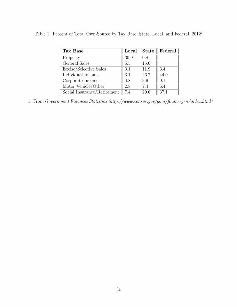
Table 1: Percent of Total Own-Source by Tax Base, State, Local, and Federal, 20121

Tax Base Local State Federal

Property 30.9 0.8General Sales 5.5 15.6Excise/Selective Sales 3.1 11.9 3.4Individual Income 3.1 26.7 44.0Corporate Income 0.8 3.9 9.1Motor Vehicle/Other 2.8 7.4 6.4Social Insurance/Retirement 7.4 29.6 37.1

1. From Government Finances Statistics (http://www.census.gov/govs/financegen/index.html)

31

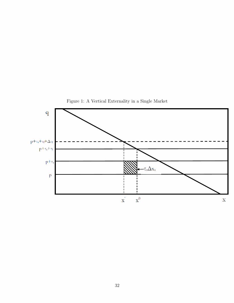
Figure 1: A Vertical Externality in a Single Market

32

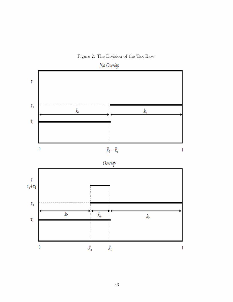
Figure 2: The Division of the Tax Base

33

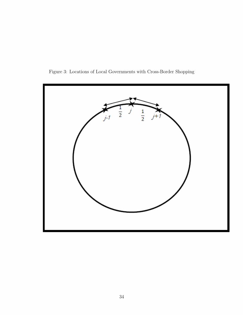
Figure 3: Locations of Local Governments with Cross-Border Shopping

34

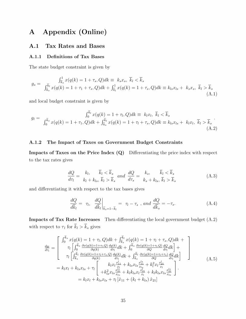
A Appendix (Online)

A.1 Tax Rates and Bases

A.1.1 Definitions of Tax Bases

The state budget constraint is given by

gs =

´ 1ksx(q(k) = 1 + τs, Q)dk ≡ ksxs, kl < ks´ kl

ksx(q(k) = 1 + τ1 + τs, Q)dk +

´ 1klx(q(k) = 1 + τs, Q)dk ≡ klsxls + ksxs, kl > ks

(A.1)

and local budget constraint is given by

gl =

´ kl0x(q(k) = 1 + τl, Q)dk ≡ klxl, kl < ks´ ks

0x(q(k) = 1 + τ1, Q)dk +

´ klksx(q(k) = 1 + τl + τs, Q)dk ≡ klsxls + klxl, kl > ks

.

(A.2)

A.1.2 The Impact of Taxes on Government Budget Constraints

Impacts of Taxes on the Price Index (Q) Differentiating the price index with respect

to the tax rates gives

dQ

dτl=

kl, kl < ks

kl + kls, kl > ksand

dQ

dτs=

ks, kl < ks

ks + kls, kl > ks(A.3)

and differentiating it with respect to the tax bases gives

dQ

dkl= τl,

dQ

dkl

∣∣∣∣ks=1−kl

= τl − τs , anddQ

dks= −τs. (A.4)

Impacts of Tax Rate Increases Then differentiating the local government budget (A.2)

with respect to τ l for kl > ks gives

dgldτl

=

´ ks0x(q(k) = 1 + τl, Q)dk +

´ klksx(q(k) = 1 + τl + τs, Q)dk +

τl

[´ ks0

∂x(q(k)=1+τl,Q)∂q(k)

dq(k)dτl

dk +´ ks0

∂x(q(k)=1+τl,Q)∂Q

dQdτldk]

+

τl

[´ klks

∂x(q(k)=1+τl+τs,Q)

∂q(k)dq(k)dτl

dk +´ klks

∂x(q(k)=1+τl+τs)∂Q

dQdτldk]

= klxl + klsxls + τl

[klxl

xl11xl

+ klsxlsxls11xls

+ k2l xlxl21xl

+k2lsxlsxls21xls

+ klklsxlxl21xl

+ klklsxlsxls21xls

].

= klxl + klsxls + τl [x̂11 + (kl + kls) x̂21]

(A.5)

35

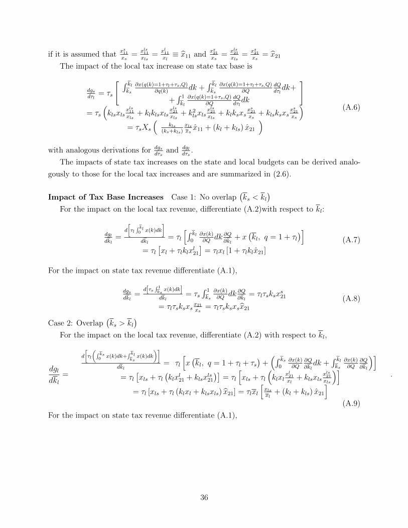
if it is assumed thatxs11xs

=xls11xls

=xl11xl≡ x̂11 and

xs21xs

=xls21xls

=xs21xs

= x̂21

The impact of the local tax increase on state tax base is

dgsdτl

= τs

[ ´ klks

∂x(q(k)=1+τl+τs,Q)∂q(k)

dk +´ klks

∂x(q(k)=1+τl+τs,Q)

∂QdQdτldk+

+´ 1kl

∂x(q(k)=1+τs,Q)∂Q

dQdτldk

]= τs

(klsxls

xls11xls

+ klklsxlsxls21xls

+ k2lsxlsxls21xls

+ klksxsxs21xs

+ klsksxsxs21xs

)= τsXs

(kls

(ks+kls)xlsxsx̂11 + (kl + kls) x̂21

) (A.6)

with analogous derivations for dgsdτs

and dgldτs

.

The impacts of state tax increases on the state and local budgets can be derived analo-

gously to those for the local tax increases and are summarized in (2.6).

Impact of Tax Base Increases Case 1: No overlap(ks < kl

)For the impact on the local tax revenue, differentiate (A.2)with respect to kl:

dgldkl

=d

[τl´ kl0 x(k)dk

]dkl

= τl

[´ kl0

∂x(k)∂Q

dk ∂Q∂kl

+ x(kl, q = 1 + τl

)]= τl

[xl + τlklx

l21

]= τlxl [1 + τlklx̂21]

(A.7)

For the impact on state tax revenue differentiate (A.1),

dgsdkl

=d[τs

´ 1ksx(k)dk]

dkl= τs

´ 1

ks

∂x(k)∂Q

dk ∂Q∂kl

= τlτsksxs21

= τlτsksxsx21xs

= τlτsksxsx̂21(A.8)

Case 2: Overlap(ks > kl

)For the impact on the local tax revenue, differentiate (A.2) with respect to kl,

dgl

dkl=

d

[τl

(´ ks0 x(k)dk+

´ klksx(k)dk

)]dkl

= τl

[x(kl, q = 1 + τl + τs

)+(´ ks

0∂x(k)∂Q

∂Q

∂kldk +

´ klks

∂x(k)∂Q

∂Q

∂kl

)]= τl

[xls + τl

(klx

l21 + klsx

ls21

)]= τl

[xls + τl

(klxl

xl21xl

+ klsxlsxls21xls

)]= τl [xls + τl (klxl + klsxls) x̂21] = τlxl

[xlsxl

+ (kl + kls) x̂21

] .

(A.9)

For the impact on state tax revenue differentiate (A.1),

36

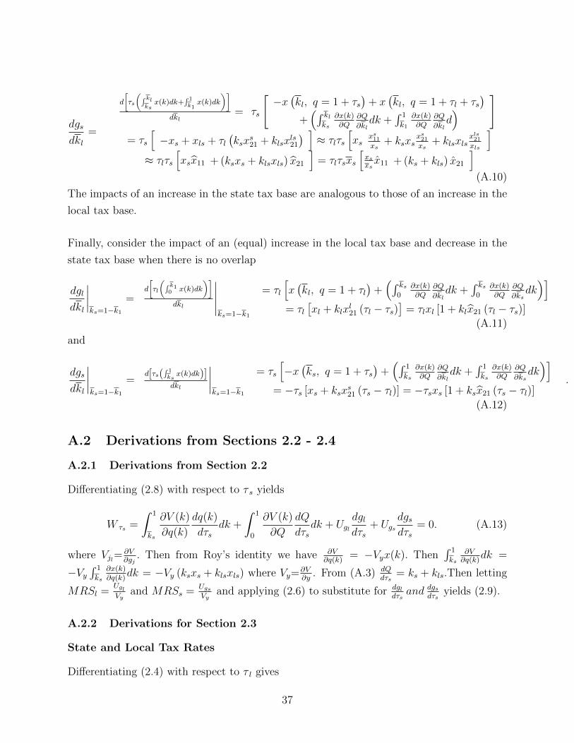
dgs

dkl=

d

[τs

(´ klksx(k)dk+

´ 1k1x(k)dk

)]dkl

= τs

[−x(kl, q = 1 + τs

)+ x

(kl, q = 1 + τl + τs

)+(´ kl

ks

∂x(k)∂Q

∂Q

∂kldk +

´ 1k1

∂x(k)∂Q

∂Q

∂kld) ]

= τs

[−xs + xls + τl

(ksx

s21 + klsx

ls21

) ]≈ τlτs

[xs

xs11xs

+ ksxsxs21xs

+ klsxlsxls21xls

]≈ τlτs

[xsx̂11 + (ksxs + klsxls) x̂21

]= τlτsxs

[xsxsx̂11 + (ks + kls) x̂21

](A.10)

The impacts of an increase in the state tax base are analogous to those of an increase in the

local tax base.

Finally, consider the impact of an (equal) increase in the local tax base and decrease in the

state tax base when there is no overlap

dgl

dkl

∣∣∣∣ks=1−k1

=d

[τl

(´ k10 x(k)dk

)]dkl

∣∣∣∣∣ks=1−k1

= τl

[x(kl, q = 1 + τl

)+(´ ks

0∂x(k)∂Q

∂Q

∂kldk +

´ ks0

∂x(k)∂Q

∂Q

∂ksdk)]

= τl[xl + klx

l21 (τl − τs)

]= τlxl [1 + klx̂21 (τl − τs)]

(A.11)

and

dgs

dkl

∣∣∣∣ks=1−k1

=d[τs(

´ 1ksx(k)dk)]

dkl

∣∣∣∣ks=1−k1

= τs

[−x(ks, q = 1 + τs

)+(´ 1

ks

∂x(k)∂Q

∂Q

∂kldk +

´ 1ks

∂x(k)∂Q

∂Q

∂ksdk)]

= −τs [xs + ksxs21 (τs − τl)] = −τsxs [1 + ksx̂21 (τs − τl)]

.

(A.12)

A.2 Derivations from Sections 2.2 - 2.4

A.2.1 Derivations from Section 2.2

Differentiating (2.8) with respect to τ s yields

W τs =

ˆ 1

ks

∂V (k)

∂q(k)

dq(k)

dτsdk +

ˆ 1

0

∂V (k)

∂Q

dQ

dτsdk + Ugl

dgldτs

+ Ugsdgsdτs

= 0. (A.13)

where Vjl=∂V∂gj. Then from Roy’s identity we have ∂V

∂q(k)= −Vyx(k). Then

´ 1

ks∂V∂q(k)

dk =

−Vy´ 1ks

∂x(k)∂q(k)

dk = −Vy (ksxs + klsxls) where Vy=∂V∂y

. From (A.3) dQdτs

= ks + kls.Then letting

MRSl =UglVy

and MRSs = UgsVy

and applying (2.6) to substitute for dgldτs

and dgsdτs

yields (2.9).

A.2.2 Derivations for Section 2.3

State and Local Tax Rates

Differentiating (2.4) with respect to τ l gives

37

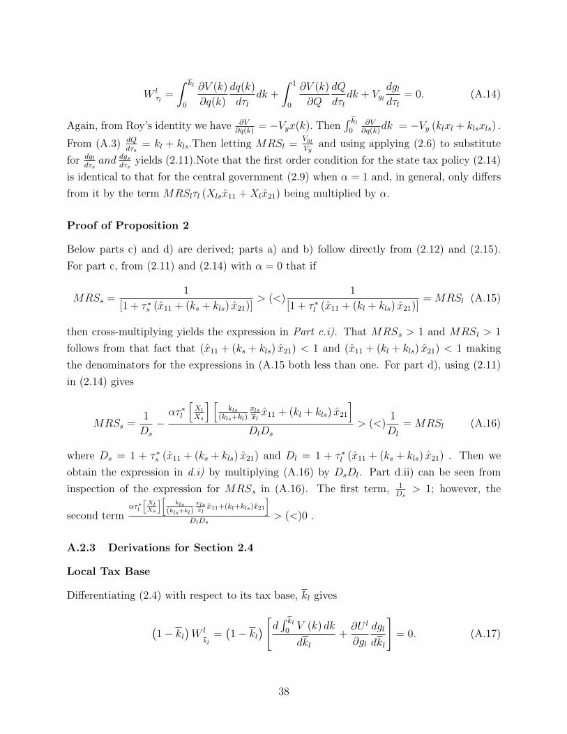
W lτl

=

ˆ kl

0

∂V (k)

∂q(k)

dq(k)

dτldk +

ˆ 1

0

∂V (k)

∂Q

dQ

dτldk + Vgl

dgldτl

= 0. (A.14)

Again, from Roy’s identity we have ∂V∂q(k)

= −Vyx(k). Then´ kl0

∂V∂q(k)

dk = −Vy (klxl + klsxls) .

From (A.3) dQdτs

= kl + kls.Then letting MRSl =VglVy

and using applying (2.6) to substitute

for dgldτs

and dgsdτs

yields (2.11).Note that the first order condition for the state tax policy (2.14)

is identical to that for the central government (2.9) when α = 1 and, in general, only differs

from it by the term MRSlτl (Xlsx̂11 +Xlx̂21) being multiplied by α.

Proof of Proposition 2

Below parts c) and d) are derived; parts a) and b) follow directly from (2.12) and (2.15).

For part c, from (2.11) and (2.14) with α = 0 that if

MRSs =1

[1 + τ ∗s (x̂11 + (ks + kls) x̂21)]> (<)

1

[1 + τ ∗l (x̂11 + (kl + kls) x̂21)]= MRSl (A.15)

then cross-multiplying yields the expression in Part c.i). That MRSs > 1 and MRSl > 1

follows from that fact that (x̂11 + (ks + kls) x̂21) < 1 and (x̂11 + (kl + kls) x̂21) < 1 making

the denominators for the expressions in (A.15 both less than one. For part d), using (2.11)

in (2.14) gives

MRSs =1

Ds

−ατ ∗l

[XlXs

] [kls

(kls+kl)xlsxlx̂11 + (kl + kls) x̂21

]DlDs

> (<)1

Dl

= MRSl (A.16)

where Ds = 1 + τ ∗s (x̂11 + (ks + kls) x̂21) and Dl = 1 + τ ∗l (x̂11 + (ks + kls) x̂21) . Then we

obtain the expression in d.i) by multiplying (A.16) by DsDl. Part d.ii) can be seen from

inspection of the expression for MRSs in (A.16). The first term, 1Ds

> 1; however, the

second termατ∗l

[XlXs

][kls

(kls+kl)xlsxlx̂11+(kl+kls)x̂21

]DlDs

> (<)0 .

A.2.3 Derivations for Section 2.4

Local Tax Base

Differentiating (2.4) with respect to its tax base, kl gives

(1− kl

)W l

kl

=(1− kl

) [d ´ kl0V (k) dk

dkl+∂U l

∂gl

dgl

dkl

]= 0. (A.17)

38

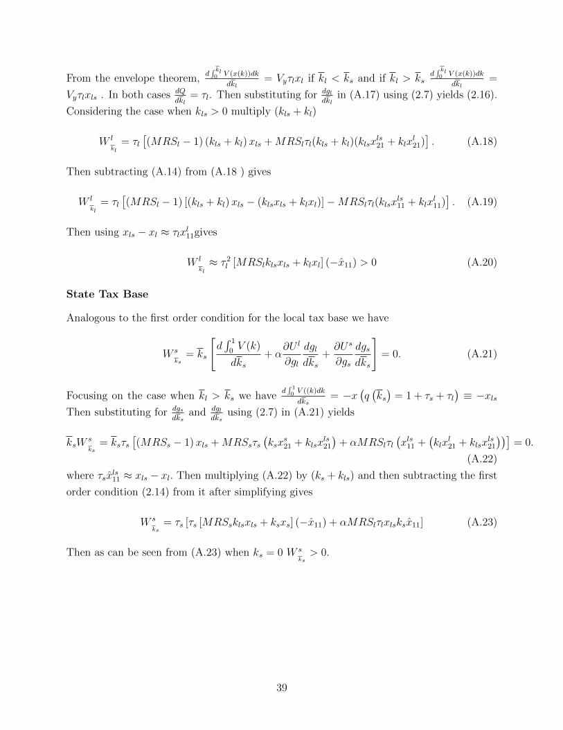
From the envelope theorem,d´ kl0 V (x(k))dk

dkl= Vyτlxl if kl < ks and if kl > ks

d´ kl0 V (x(k))dk

dkl=

Vyτlxls . In both cases dQ

dkl= τl. Then substituting for dgl

dklin (A.17) using (2.7) yields (2.16).

Considering the case when kls > 0 multiply (kls + kl)

W l

kl

= τl[(MRSl − 1) (kls + kl)xls +MRSlτl(kls + kl)(klsx

ls21 + klx

l21)]. (A.18)

Then subtracting (A.14) from (A.18 ) gives

W l

kl

= τl[(MRSl − 1) [(kls + kl)xls − (klsxls + klxl)]−MRSlτl(klsx

ls11 + klx

l11)]. (A.19)

Then using xls − xl ≈ τlxl11gives

W l

kl

≈ τ 2l [MRSlklsxls + klxl] (−x̂11) > 0 (A.20)

State Tax Base

Analogous to the first order condition for the local tax base we have

W s

ks= ks

[d´ 10V (k)

dks+ α

∂U l

∂gl

dgl

dks+∂U s

∂gs

dgs

dks

]= 0. (A.21)

Focusing on the case when kl > ks we haved´ 10 V ((k)dk

dks= −x

(q(ks)

= 1 + τs + τl)≡ −xls

Then substituting for dgsdks

and dgldks

using (2.7) in (A.21) yields

ksWs

ks= ksτs

[(MRSs − 1)xls +MRSsτs

(ksx

s21 + klsx

ls21

)+ αMRSlτl

(xls11 +

(klx

l21 + klsx

ls21

))]= 0.

(A.22)

where τsx̂ls11 ≈ xls − xl. Then multiplying (A.22) by (ks + kls) and then subtracting the first

order condition (2.14) from it after simplifying gives

W s

ks= τs [τs [MRSsklsxls + ksxs] (−x̂11) + αMRSlτlxlsksx̂11] (A.23)

Then as can be seen from (A.23) when ks = 0 W s

ks> 0.

39

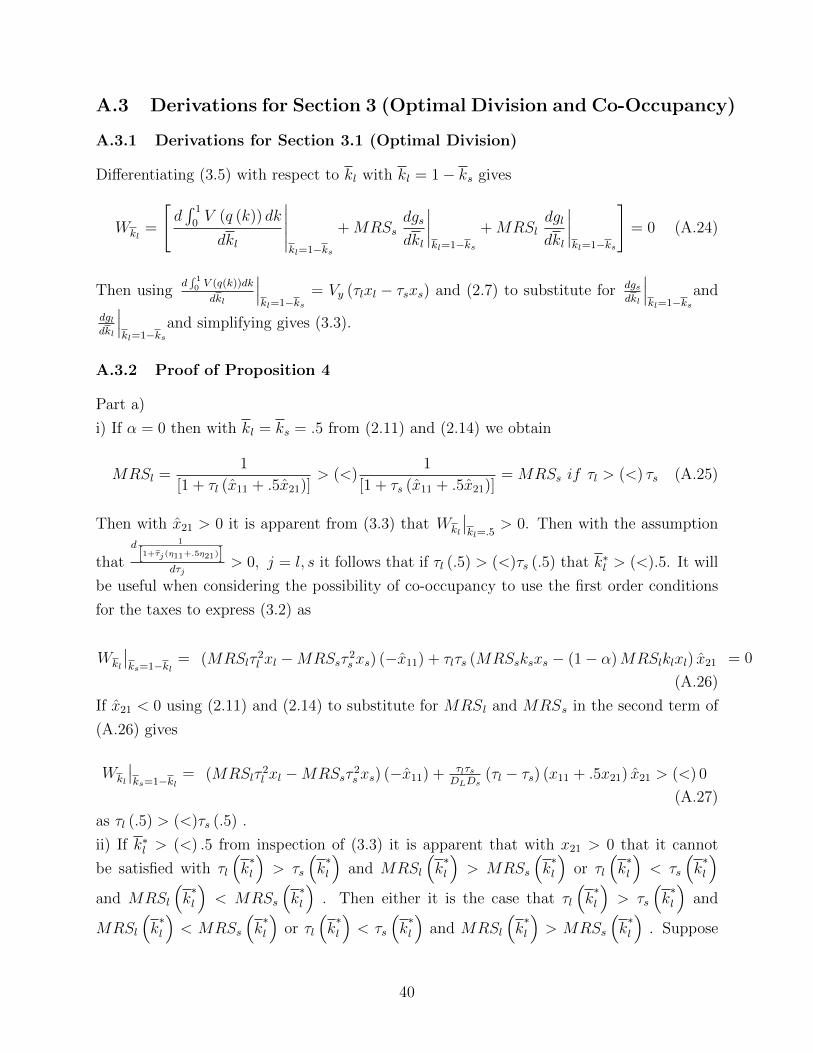
A.3 Derivations for Section 3 (Optimal Division and Co-Occupancy)

A.3.1 Derivations for Section 3.1 (Optimal Division)

Differentiating (3.5) with respect to kl with kl = 1− ks gives

Wkl=

[d´ 1

0V (q (k)) dk

dkl

∣∣∣∣∣kl=1−ks

+MRSsdgs

dkl

∣∣∣∣kl=1−ks

+MRSldgl

dkl

∣∣∣∣kl=1−ks

]= 0 (A.24)

Then usingd´ 10 V (q(k))dk

dkl

∣∣∣kl=1−ks

= Vy (τlxl − τsxs) and (2.7) to substitute for dgsdkl

∣∣∣kl=1−ks

and

dgldkl

∣∣∣kl=1−ks

and simplifying gives (3.3).

A.3.2 Proof of Proposition 4

Part a)

i) If α = 0 then with kl = ks = .5 from (2.11) and (2.14) we obtain

MRSl =1

[1 + τl (x̂11 + .5x̂21)]> (<)

1

[1 + τs (x̂11 + .5x̂21)]= MRSs if τl > (<) τs (A.25)

Then with x̂21 > 0 it is apparent from (3.3) that Wkl

∣∣kl=.5

> 0. Then with the assumption

thatd 1

[1+τ̃j(η11+.5η21)]dτj

> 0, j = l, s it follows that if τl (.5) > (<)τs (.5) that k∗l > (<).5. It will

be useful when considering the possibility of co-occupancy to use the first order conditions

for the taxes to express (3.2) as

Wkl

∣∣ks=1−kl

= (MRSlτ2l xl −MRSsτ

2s xs) (−x̂11) + τlτs (MRSsksxs − (1− α)MRSlklxl) x̂21 = 0

(A.26)

If x̂21 < 0 using (2.11) and (2.14) to substitute for MRSl and MRSs in the second term of

(A.26) gives

Wkl

∣∣ks=1−kl

= (MRSlτ2l xl −MRSsτ

2s xs) (−x̂11) + τlτs

DLDs(τl − τs) (x11 + .5x21) x̂21 > (<) 0

(A.27)

as τl (.5) > (<)τs (.5) .

ii) If k∗l > (<) .5 from inspection of (3.3) it is apparent that with x21 > 0 that it cannot

be satisfied with τl

(k∗l

)> τs

(k∗l

)and MRSl

(k∗l

)> MRSs

(k∗l

)or τl

(k∗l

)< τs

(k∗l

)and MRSl

(k∗l

)< MRSs

(k∗l

). Then either it is the case that τl

(k∗l

)> τs

(k∗l

)and

MRSl

(k∗l

)< MRSs

(k∗l

)or τl

(k∗l

)< τs

(k∗l

)and MRSl

(k∗l

)> MRSs

(k∗l

). Suppose

40

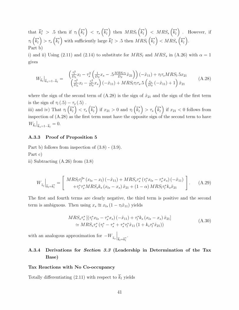
that k∗l > .5 then if τl

(k∗l

)< τs

(k∗l

)then MRSl

(k∗l

)< MRSs

(k∗l

). However, if

τl

(k∗l

)> τs

(k∗l

)with sufficiently large k∗l > .5 then MRSl

(k∗l

)< MRSs

(k∗l

).

Part b)

i) and ii) Using (2.11) and (2.14) to substitute for MRSl and MRSs in (A.26) with α = 1

gives

Wkl

∣∣ks=1−kl

=

(τ2lDLxl − τ 2s

(1DSxs − .5MRSlτl

DSx̂21

))(−x̂11) + τlτsMRSl.5x21(

τ2lDLxl − τ2s

DSxs

)(−x̂11) +MRSlτlτs.5

(τsDS

(−x̂11) + 1)x̂21

(A.28)

where the sign of the second term of (A.28) is the sign of x̂21 and the sign of the first term

is the sign of τl (.5)− τs (.5) .

iii) and iv) That τl

(k∗l

)< τs

(k∗l

)if x21 > 0 and τl

(k∗l

)> τs

(k∗l

)if x21 < 0 follows from

inspection of (A.28) as the first term must have the opposite sign of the second term to have

Wkl

∣∣ks=1−kl

= 0.

A.3.3 Proof of Proposition 5

Part b) follows from inspection of (3.8) - (3.9).

Part c)

ii) Subtracting (A.26) from (3.8)

Wkl

∣∣∣kl=k

∗l

=

[MRSlτ

2∗l (xls − xl) (−x̂11) +MRSsτ

∗s (τ ∗l xls − τ ∗s xs) (−x̂11)

+τ ∗l τ∗sMRSsks (xls − xs) x̂21 + (1− α)MRSlτ

∗l ksx̂21

]. (A.29)

The first and fourth terms are clearly negative, the third term is positive and the second

term is ambiguous. Then using xs u xls (1− τlx̂11) yields

MRSsτ∗s [(τ ∗l xls − τ ∗s xs) (−x̂11) + τ ∗l ks (xls − xs) x̂21]

'MRSsτ∗s (τ ∗l − τ ∗s + τ ∗s τ

∗l x̂11 (1 + ksτ

∗l x̂21))

(A.30)

with an analogous approximation for −Wks

∣∣∣kl=k

∗l

.

A.3.4 Derivations for Section 3.3 (Leadership in Determination of the Tax

Base)

Tax Reactions with No Co-occupancy

Totally differentiating (2.11) with respect to kl yields

41

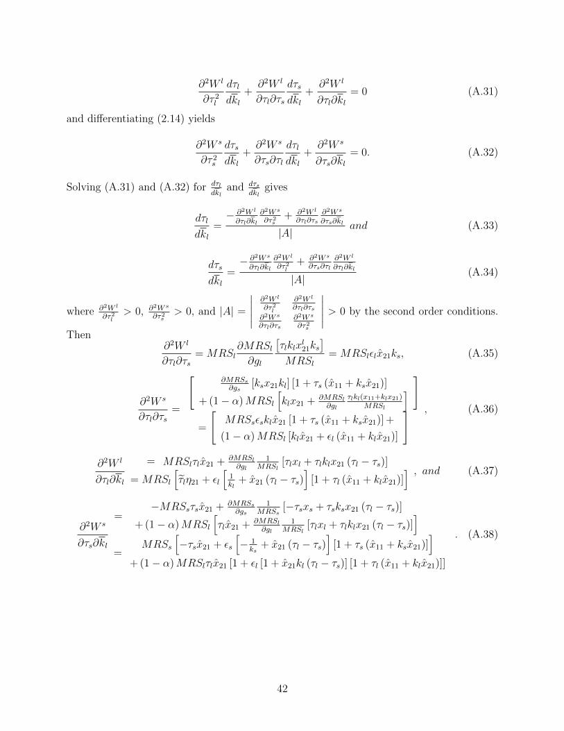
∂2W l

∂τ 2l

dτl

dkl+∂2W l

∂τl∂τs

dτs

dkl+∂2W l

∂τl∂kl= 0 (A.31)

and differentiating (2.14) yields

∂2W s

∂τ 2s

dτs

dkl+∂2W s

∂τs∂τl

dτl

dkl+∂2W s

∂τs∂kl= 0. (A.32)

Solving (A.31) and (A.32) for dτldkl

and dτsdkl

gives

dτl

dkl=− ∂2W l

∂τl∂kl

∂2W s

∂τ2s+ ∂2W l

∂τl∂τs∂2W s

∂τs∂kl

|A|and (A.33)

dτs

dkl=− ∂2W s

∂τl∂kl

∂2W l

∂τ2l+ ∂2W s

∂τs∂τl

∂2W l

∂τl∂kl

|A|(A.34)

where ∂2W l

∂τ2l> 0, ∂2W s

∂τ2s> 0, and |A| =

∣∣∣∣∣ ∂2W l

∂τ2l

∂2W l

∂τl∂τs∂2W s

∂τl∂τs∂2W s

∂τ2s

∣∣∣∣∣ > 0 by the second order conditions.

Then∂2W l

∂τl∂τs= MRSl

∂MRSl∂gl

[τlklx

l21ks

]MRSl

= MRSlεlx̂21ks, (A.35)

∂2W s

∂τl∂τs=

[∂MRSs∂gs

[ksx21kl] [1 + τs (x̂11 + ksx̂21)]

+ (1− α)MRSl

[klx21 + ∂MRSl

∂gl

τlkl(x11+klx21)MRSl

] ]

=

[MRSsεsklx̂21 [1 + τs (x̂11 + ksx̂21)] +

(1− α)MRSl [klx̂21 + εl (x̂11 + klx̂21)]

] , (A.36)

∂2W l

∂τl∂kl

= MRSlτlx̂21 + ∂MRSl∂gl

1MRSl

[τlxl + τlklx21 (τl − τs)]= MRSl

[τ̃lη21 + εl

[1kl

+ x̂21 (τl − τs)]

[1 + τl (x̂11 + klx̂21)]] , and (A.37)

∂2W s

∂τs∂kl

=−MRSsτsx̂21 + ∂MRSs

∂gs1

MRSs[−τsxs + τsksx21 (τl − τs)]

+ (1− α)MRSl

[τlx̂21 + ∂MRSl

∂gl

1MRSl

[τlxl + τlklx21 (τl − τs)]]

=MRSs

[−τsx̂21 + εs

[− 1ks

+ x̂21 (τl − τs)]

[1 + τs (x̂11 + ksx̂21)]]

+ (1− α)MRSlτlx̂21 [1 + εl [1 + x̂21kl (τl − τs)] [1 + τl (x̂11 + klx̂21)]]

. (A.38)

42

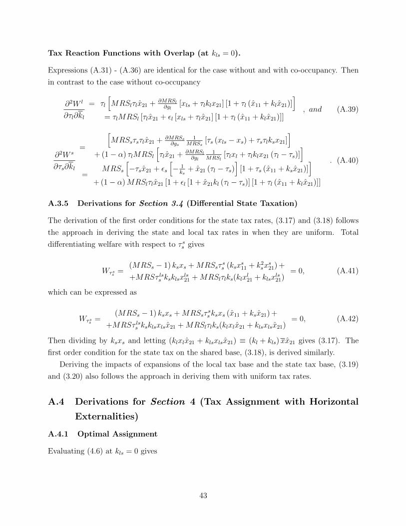
Tax Reaction Functions with Overlap (at kls = 0).

Expressions (A.31) - (A.36) are identical for the case without and with co-occupancy. Then

in contrast to the case without co-occupancy

∂2W l

∂τl∂kl

= τl

[MRSlτlx̂21 + ∂MRSl

∂gl[xls + τlklx21] [1 + τl (x̂11 + klx̂21)]

]= τlMRSl [τlx̂21 + εl [xls + τlx̂21] [1 + τl (x̂11 + klx̂21)]]

, and (A.39)

∂2W s

∂τs∂kl

=

[MRSsτsτlx̂21 + ∂MRSs

∂gs1

MRSs[τs (xls − xs) + τsτlksx21]

]+ (1− α) τlMRSl

[τlx̂21 + ∂MRSl

∂gl

1MRSl

[τlxl + τlklx21 (τl − τs)]]

=MRSs

[−τsx̂21 + εs

[− 1ks

+ x̂21 (τl − τs)]

[1 + τs (x̂11 + ksx̂21)]]

+ (1− α)MRSlτlx̂21 [1 + εl [1 + x̂21kl (τl − τs)] [1 + τl (x̂11 + klx̂21)]]

. (A.40)

A.3.5 Derivations for Section 3.4 (Differential State Taxation)

The derivation of the first order conditions for the state tax rates, (3.17) and (3.18) follows

the approach in deriving the state and local tax rates in when they are uniform. Total

differentiating welfare with respect to τ ss gives

Wτss =(MRSs − 1) ksxs +MRSsτ

ss (ksx

s11 + k2sx

s21) +

+MRSτ lss ksklsxls21 +MRSlτlks(klx

l21 + klsx

ls21)

= 0, (A.41)

which can be expressed as

Wτss =(MRSs − 1) ksxs +MRSsτ

ss ksxs (x̂11 + ksx̂21) +

+MRSτ lss ksklsxlsx̂21 +MRSlτlks(klxlx̂21 + klsxlsx̂21)= 0, (A.42)

Then dividing by ksxs and letting (klxlx̂21 + klsxlsx̂21) ≡ (kl + kls)xx̂21 gives (3.17). The

first order condition for the state tax on the shared base, (3.18), is derived similarly.

Deriving the impacts of expansions of the local tax base and the state tax base, (3.19)

and (3.20) also follows the approach in deriving them with uniform tax rates.

A.4 Derivations for Section 4 (Tax Assignment with Horizontal

Externalities)

A.4.1 Optimal Assignment

Evaluating (4.6) at kls = 0 gives

43

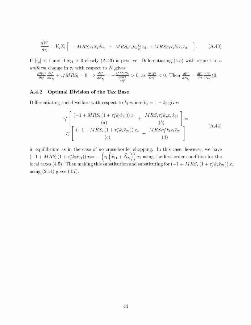
dW

dτl= VyXl

[−MRSlτlXlN̂τl + MRSsτsks

xsxlx̂21 +MRSlτlτsksτ̂sx̂21

]. (A.43)

If |τ̂s| < 1 and if x̂21 > 0 clearly (A.43) is positive. Differentiating (4.5) with respect to a

uniform change in τ l with respect to N̂τlgives∂2W l

∂τ2l

dτ∗ldN̂τl

+ τ ∗l MRSl = 0 ⇒ dτ∗ldN̂τl

= − τ∗l MRSl∂2Wl

∂τ2l

> 0. as ∂2W l

∂τ2l< 0. Then dW

dN̂τl= dW

dτl

dτ∗ldN̂τl

¿0.

A.4.2 Optimal Division of the Tax Base

Differentiating social welfare with respect to kl where ks = 1− kl gives

τ ∗l

[(−1 +MRSl (1 + τ ∗l klx̂21))xl

(a)+

MRSsτ∗s ksxsx̂21

(b)

]=

τ ∗s

[(−1 +MRSs (1 + τ ∗s ksx̂21))xs

(c)+

MRSlτ∗l klxlx̂21

(d)

] (A.44)

in equilibrium as in the case of no cross-border shopping. In this case, however, we have

(−1 +MRSl (1 + τ ∗l klx̂21))xl= −(τl

(x̂11 + N̂τl

))xl using the first order condition for the

local taxes (4.5). Then making this substitution and substituting for (−1 +MRSs (1 + τ ∗s ksx̂21))xs

using (2.14) gives (4.7).

44