The Application of Exact Cover to the Creating of Sudoku Puzzle

Team # 3140 Page 1 of 24

The Application of Exact Cover to the

Creating of Sudoku Puzzle

Summary In this paper, we develop an algorithm to create a Sudoku puzzle of a

desired difficulty level. The main of our work is the algorithm to simulate the

procedure when people are solving a Sudoku problem. We build the exact

cover model to make the rules in filling a Sudoku puzzle clear, and establish a

series of theorems in the general exact cover problem to imitate the

techniques people used in the Sudoku problem of the exact cover version.

We have four integrate algorithms: a speed solver, a simulation solver, a

Sudoku generator and a Sudoku generator to meet a desired difficulty level.

The speed solver has already developed by Donald E. Knuth known as “Dancing

Links” and, as far as we see, need not to be improved. The simulation solver is

based on the theorems developed by ourselves, and the complexity is

minimized by several methods. The speed of our simulation solver is much

faster than that of trying the techniques in an original Sudoku puzzle. The two

generators is not the center of our algorithm, so their algorithms may be

familiar.

Another important part in this paper is the difficulty rating system. The

system is determined by four axioms which are induced from the experience.

Introduction A typical Sudoku puzzle is a 9×9 grid with some of the cells (see definition

of cell in next section) filled with the digits from 1 to 9, and the goal is to

complete the grid so that every row, column and block (see definition of block

in next section) contains each of the digits exactly once.

The Arabic digits 1-9 here can be replaced by any other nine different

symbols, and the size of the grid can also be extended to a n2 × n2 case.

In our model, only the 9×9 case will be discussed. Considering the similarity

of narration, letters a-i are used to represent the nine rows of a Sudoku, while

symbols 1-9 to the nine columns.

Terminologies of Sudoku Puzzles Cell: One of the 81 boxes in the Sudoku grid.

Block: The outlined 3×3 sub-grid of the main grid. We will refer to


a block with its row and column, e.g. block def456 includes

squares d4, d5, d6, e4, e5, e6, f4, f5 and f6.

Unit: Each row, column and block is a unit of a Sudoku grid and a

cell’s unit refers to an arbitrary unit which the cell belongs

to.

Neighborhood: A cell A’s neighborhood refers to the 3 units (as a whole)

that A belongs to.

Buddy: A cell A’s buddy refers to a cell in A’s neighborhood.

Valid Solution: When there is only one method to fill all the cells in a

Sudoku, then we say the Sudoku puzzle has a valid

solution.

Candidate: The numbers that don’t appear in a cell A’s neighborhood

is called the candidates of A. Analogous terminology as

candidates of a unit is also used.

Technique:

(see Appendix 1)

A method used to eliminate the candidates of a cell in an

unique circumstance. In next section we will illustrate that

there always exists at least one technique that can

eliminate the candidates of a unique cell.

Operation: The process of using a kind of techniques to eliminate as

many candidates as possible from one or more cells.

Table 1

Symbols and their meanings

R(A) The row cell A belongs to

C(A) The column cell A belongs to

Bl(A) The block cell A belongs to

U(A) Arbitrary one of R(A), C(A) and B(A)

O(A) Cell A’s neighborhood

Bu(A) A cell belongs to cell A’s neighborhood

Can(A) All candidates of cell A

Model Construction

The exact cover problem

For the sake of minimizing the complexity of our algorithm, we use

exact-cover-speak to reformulate the Sudoku problem. The matrix

representation of the exact cover problem [9] is like this: Given a binary


matrix (with all entries 0 or 1), choose a collection of rows from the

row-arrays set of the matrix such that exact one 1 in each column appears in

these rows. In another word, the selected row arrays sum to a row array

with all element 1.

Application to the Sudoku problem

Actually, the columns of the matrix discussed above are constraints in

the selection, that is, exact one from the rows in which the 1s in a single

column appear is added to the row collection. The constraints coincide with

the rules that must be obeyed while filling the Sudoku problem.

The rows that we will select are about digits and the cells where they are

placed. So we use the triple (i, j, k) to label the rows, which represents the

digit k is filled in the cell of row i and column j. Hence we have 9×9×9=729

rows.

There are four types of constraints: one cell can only contain one digit,

there is exact one instance for each digit in each row, each column and each

block. For example, only one among 1 to 9 can be filled in (1, 1). So in the

corresponding column, elements in row (1, 1, 1), (1, 1, 2)…, (1, 1, 9) are 1

while others are 0. We have got 4×9×9=324 columns. The Sudoku matrix

has been created, and we call it A from now on. (There is a sample for the

corresponding matrix for a 4×4 Sudoku problem in the Appendix 2.) Each

row in A has four 1s, for there are four constraints on each digit in each cell.

Each column in A has nine 1s.

Algorithm

The purpose

Some of the numbers are given in the Sudoku problem, that is, some of

the rows in our matrix have been selected. The goal is to select the other

rows. When a row r is selected, the constraints about this row are useless,

and the other row involved in these constraints can never be selected. So

once we make a selection, delete the selected row, delete all columns

intersect with this row (a column and a row is said to be intersect when the

intersect element is 1), and delete all rows intersect with these columns.

Use A-r to represent the matrix after being modified.

Previous algorithms

A solving algorithm called “Algorithm X” [9] has been developed by

Donald E. Knuth, and “Dancing Links” [9] by himself makes great


improvement on “Algorithm X” by the notion of a more efficient protection

of the scene while doing the recursion. The advantage of both these two

algorithm is that for every element 1 in the matrix A they mark the nearest

element 1 on its left, right, up and down, so they can find the useful

constraints in the matrix A faster.

We also use this link method to improve our algorithm. Our purpose is

to measure the difficulty of a certain Sudoku, so we have to translate human

techniques in Sudoku playing into the exact cover problem terminology.

Algorithm in the exact cover problem

Definitions and notations

R is the set of all row arrays of A.

C is the set of all column arrays of A.

A r, c is the element in row r and column c of A.

For r ∈ R, N r : = c ∈ C|A r, c = 1 .

For c ∈ C, N c : = r ∈ R|A r, c = 1 .

For R0 ⊆ R,

N R0 : = N r

r∈R0

For C0 ⊆ C,

N C0 : = N c

c∈C0

Sol A represents the final collection of rows.

Some simple propositions

Proposition 1: r ∈ N c if and only if c ∈ N(r).

Proposition 2: r ∈ N N r0 if and only if N(r) ∩ N r0 ≠ ∅.

Proposition 3: If c ∈ C, N c = 0, then no solution.

Proposition 4: If r ∈ R is selected, then columns N r and rows

N N r will be deleted from A.

Main results

Theorem 5: If r ∈ R, c ∈ C, N c = r ,

then Sol A = r ∪ Sol A − r .

Theorem 6: If c1 ≠ c2 ∈ C, N c1 ⊆ N c2 , r ∈ N c2 \N c1 ,


then Sol A = Sol A − r .

Theorem 7: r1, r2, r3, r4 ∈ R(different from each other),

c1 ≠ c2 ∈ C, N c1 = r1, r2 , N c2 = r3, r4 ,

N r1 ∩ N r3 ≠ ∅, N r2 ∩ N r4 ≠ ∅,

If r ∈ N N r1 ⋂N N r3 , r ≠ r1, r ≠ r3,


Proof: N c1 = r1, r2 , so r1 or r2 ∈ Sol A

if r2 ∈ Sol A

for N r2 ∩ N r4 ≠ ∅,

there is a column intersect both r2 or r4,

so r4 ∉ Sol A ,

since N c2 = r3 , r4 ,

r3 ∈ Sol A

so either r1 or r3 ∈ Sol A

if r ∈ N N r1 ⋂N N r3 , then r ∈ N N r1 and r ∈ N N r3

by Proposition 2, N(r) ∩ N r1 ≠ ∅ or N(r) ∩ N r3 ≠ ∅, that is,

r and r1 can not both ∈ Sol A , r and r3 can not both ∈ Sol A

for either r1 or r3 ∈ Sol A , r ∉ Sol A □

Theorem 8: r1, r2,… , r9 ∈ R(different from each other),

c1, c2, c3 ∈ C(different from each other),

N c1 ⊆ r1, r2, r3 , N c2 ⊆ r4, r5, r6 ,

N c3 ⊆ r7, r8, r9 ,

N r1 ∩ N r4 ∩ N r7 ≠ ∅,

N r2 ∩ N r5 ∩ N r8 ≠ ∅,

N r3 ∩ N r6 ∩ N r9 ≠ ∅,

If r ∈ N N r1 ⋂N N r4 ⋂N N r7 ,

and r ≠ r1, r ≠ r4, r ≠ r7,


Theorem 9: r1, r2,… , r8 ∈ R(different from each other),

c1, c2, c3, c4 ∈ C(different from each other),

N c1 = r1, r2 , N c2 = r3, r4 ,

N c3 = r5, r6 , N c4 ⊇ r7, r8 ,

N r1 ∩ N r3 ≠ ∅, N r3 ∩ N r5 ≠ ∅,

N r5 ∩ N r7 ≠ ∅, N r7 ∩ N r1 ≠ ∅,

N r2 ∩ N r4 ≠ ∅, N r4 ∩ N r6 ≠ ∅,


N r6 ∩ N r8 ≠ ∅, N r8 ∩ N r2 ≠ ∅,

then Sol A = Sol A − r7 , Sol A = Sol A − r8 .

Relation to the Sudoku problem

Let’s see the relation between the former theorems and techniques

used in the Sudoku problem.

In Theorem 5, if c is the constraint that one cell can only contain one

digit, there is only one candidate for the corresponding cell. The

conclusion coincides with the technique “Naked Singles”. If c is of other

types, the theorem is same to “Hidden Singles”.

In Theorem 6, if c1 is about block singularity and c2 is about row

or column singularity, the corresponding technique is “Locked

Candidates”.

Theorem 7 has many variations that lead to different types of

techniques. For example, if c1 is the constraint that the digit k appears

in row i once, c2is that the digit l appears in row i once,

r1 = i, j1 , k , r2 = i, j2, k , r3 = i, j1, l , and r4 = i, j2, l ,

then for m ≠ k, l , i, j1, m ∈ N N r1 ⋂N N r3 should be

eliminated from the matrix. It is “Hidden Pairs”. For certain types of c1

and c2, Theorem 7 can also be “Naked Pairs” and “X-wing”(see the

difficulty rating diagram in the following section).

The reason why theorem 7 can cause several types of techniques is

that the exact cover methods ignore the difference between the 4 types

of constraints. To tell the difference between these human techniques

is also easy, only need to know what type of constrains the column is. In

the difficulty rating system, techniques generated from same theorem

can have different score but should not be in great difference.

Theorem 8 is similar from Theorem 7. It leads to “Naked Triples”,

“Hidden Triples”, “Swordfish”, “XY-wing” and “XYZ-wing”.

Theorem 9 comes from the hypothesis that the Sudoku problem has

a unique solution and is derived from the technique “Unique Solution

Constraint” with generalization.

There are also other techniques such as “XY-Chain”, “Simple

Coloring”, “Multi Coloring”, “Remote Naked Pairs” and “Forcing Chain”.

From our point of view, they are of same type by ignoring the type of

constraints. We regard them as a simple form of “Try and False” or

“Guess”, just as the depth-first backtracks in the algorithm “Dancing

Links”.


How to use the theorems in the algorithm

To use these theorems in the algorithm, we need not to try all the

possible combinations of the columns. Noting that each column

concerned in these theorems (except Theorem 6) has a maximal

number of 1s, we can diminish our scope to all the columns with, for

example in Theorem 8, three 1s. Then check all the combinations from

the columns in our scope. After the columns are selected, the rows

included in the theorems are definite except for their order. Check the

condition for every order. Finally, we can apply the theorem so that we

can rule out or select some rows.

Algorithm in the solver and the generator

The solver

1. get selected rows from the given numbers in the Sudoku problem;

2. deleted the selected rows, the columns intersect with these rows

and the rows intersect with these columns from the matrix;

3. if (there is not any column left)

we have solved the Sudoku;

4. apply Theorem 5;

if (make change)

if (difficulty rate of this step > current difficulty)

current difficulty = difficulty rate of this step;

if (difficulty rate of this step > desired difficulty)

save (the cell related to the selected row);

repeat step 2;

5. apply Theorem 6;

if (make change)




save (the cell related to the deleted row);

repeat step 4;

6. apply Theorem 7;

if (make change)






repeat step 4;

7. apply Theorem 8;

if (make change)





repeat step 4;

8. apply Theorem 9;

if (make change)





repeat step 4;

9. current difficulty = extreme; save (all unfilled cell);

The generator

To generate a random full Sudoku:

1. Fill the up left block with 1 to 9 ordering. Change row order

randomly, then column order randomly.

2. Fill the first row with digits that have not been used in the first row

of the up left block. Change the newly-written-in six digits by

random order. Fill the first column with digits that have not been

used in the first column of the up left block. Change the

newly-written-in six digits by random order.

3. Fill the remains by “Dancing Links”. (A theorem guarantee that this

can always be done)

To generate a Sudoku problem:

1. Generate a random full Sudoku.

2. Randomly choose a filled cell. Delete the digit in the cell. Check

whether the Sudoku has multiple solutions by “Dancing Links”. If

has, fill the deleted number back and we get a Sudoku problem. If

not, repeat this step.

Our generating procedure is as follow:

1. Generate a random Sudoku problem.

2. Test its difficulty level by our solver, store the over difficult steps.


3. If it is harder than what is required, fill one of the cells involve in the

over difficult steps and repeat step 2. If it is too easy, repeat step 1.

4. Obtain the Sudoku problem with difficulty level desired.

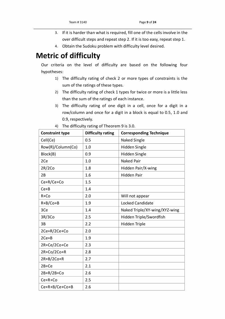
Metric of difficulty Our criteria on the level of difficulty are based on the following four

hypotheses:

1) The difficulty rating of check 2 or more types of constraints is the

sum of the ratings of these types.

2) The difficulty rating of check 1 types for twice or more is a little less

than the sum of the ratings of each instance.

3) The difficulty rating of one digit in a cell, once for a digit in a

row/column and once for a digit in a block is equal to 0.5, 1.0 and

0.9, respectively.

4) The difficulty rating of Theorem 9 is 3.0.

Constraint type Difficulty rating Corresponding Technique

Cell(Ce) 0.5 Naked Single

Row(R)/Column(Co) 1.0 Hidden Single

Block(B) 0.9 Hidden Single

2Ce 1.0 Naked Pair

2R/2Co 1.8 Hidden Pair/X-wing

2B 1.6 Hidden Pair

Ce+R/Ce+Co 1.5

Ce+B 1.4

R+Co 2.0 Will not appear

R+B/Co+B 1.9 Locked Candidate

3Ce 1.4 Naked Triple/XY-wing/XYZ-wing

3R/3Co 2.5 Hidden Triple/Swordfish

3B 2.2 Hidden Triple

2Ce+R/2Ce+Co 2.0

2Ce+B 1.9

2R+Ce/2Co+Ce 2.3

2R+Co/2Co+R 2.8

2R+B/2Co+R 2.7

2B+Ce 2.1

2B+R/2B+Co 2.6

Ce+R+Co 2.5

Ce+R+B/Ce+Co+B 2.6


R+Co+B 2.9

Unique 3.0 Unique Solution Constraint

The difficulty rating of the Sudoku problem is the rating of the hardest step.

Extensibility

The difficulty rating criteria discussed above have great extensibility from

which we can derive a varying number of difficulty levels. For example, we can

get a 5-level metric by setting:

Very easy: 0.5

Easy: 0.6-1.5

Medium: 1.6-2.3

Hard: 2.4-3.0

Extreme: Can not be solved by the theorems.

Complexity

Methods to minimize the complexity for a second time

· For every 1 in the exact cover matrix, link it to the nearest 1 on its left,

right, up and down. We do not take any notice on the 0s in the matrix.

So such links allow us to search the next 1 faster. Another reason is that,

we can apply the same method in “Dancing Links” to our algorithm.

· We have labeled the rows in the matrix like (i, j, k). In the computer

program, we can label it by r=81i+9j+k. So i=[r/81], j=[r/9]%9 and k=r%9

(where the notation [a] means the greatest integer less than or equal to

a and the notation b%c means the residue when b is divided by c).

· We also can make an assumption about the label of the columns in the

matrix. First we label

(0, i, j) for the constraint that the cell (i, j) can only contain one

digit

(1, i, k) for the constraint that there are exact one instance for k in

row i

(2, j, k) for the constraint that there are exact one instance for k in

column j

(3, b, k) for the constraint that there are exact one instance for k in

block b

Then labels in the computer program is follow the same rule as those

about the rows.

Time complexity


The complexity of our algorithm consists of 4 parts:

1) The complexity of N ∙ operation.

2) The expectation of times N ∙ operation used in the itineration

of each theorem.

3) The expectation of times each theorem used in solving a single

Sudoku problem.

4) The expectation of times of generating a new Sudoku problem

to obtain a desired difficulty level.

The complexity of the first three parts is hard to be calculated for the

reason that the scale of our algorithm is smaller and smaller while the

algorithm is running and the decrease of the scale is not a constant even for

a single theorem. However, the expectation of such complexity can be

obtained by getting statistics from repeating the algorithm.

The fourth part can be calculated. Supposing that we have n difficult

levels, and the possibility of having a level i after generating a random

Sudoku problem is ai. Also supposing that the possibility of getting a level j

problem from a level i problem by fill one of the cells involve in the over

difficult steps is bij , the possibility of getting a level j from a level i in m step

is bij m

. Then the matrix bij m = bij

m. The possibility of getting j from i

from the first time in m step, cij m

= bij m

− bij m−1

bjj . The possibility of

getting j from i, cij = cij m 81

m=1 . The expectation of the times of generating

new puzzle is

ai k 1 − cij k−1

cij

∞

k=1

n

i=1

= aicij−1

n

i=1

.

The expectation of the times of using our solver after each generation

except the last is

ai m cik m

− cil m−1

clk

n

l=j+1

81

m=1

j−1

k=1

n

i=1

.

The expectation of the times of using our solver after the last generation is

ai mcij m

81

m=1

n

i=1

Hence the expectation of the total times of using our solver in a single

generation for a certain difficulty level j is


ai m cik m

− cil m−1

clk

n

l=j+1

81

m=1

j−1

k=1

n

i=1

∗ aicij−1

n

i=1

− 1 + ai mcij m

81

m=1

n

i=1

.

by Wald Lemma. Since all ai and bij can be obtained by using the

frequency gaining from repeating the generating and measure procedure,

all of the value given by formulae above can be calculated.

Space complexity

To generate the Sudoku and justify whether the Sudoku have unique

solution, we use the “Dancing Links” which is suggested by Donald Knuth to

efficiently implement his “Algorithm X”. It is a recursive, nondeterministic,

depth-first, brute-force algorithm. To apply “Dancing Links” in Sudoku, we

first generate the 729×324 matrix with all constrains as mentioned before.

This matrix is a sparse matrix, which is a matrix populated primarily with

zeros, with only 2916(4×729 or 9×324) 1s, while others are 0s. So the

number of 1s is much smaller than the number of all the entries in the

matrix which equal to 236196(729×324). The “Dancing Links” algorithm only

store the 1s of the matrix by using the circular doubly linked list. Hence it

saves lots of space. The space complexity of our algorithm is very small since

we only need to save 2916 1s.

Strength and weakness

Strength points

· We combine the exact cover problem and the human techniques so

that we are able to imitate the efficient algorithm “Dancing Links” to

achieve a fast human simulation solver of our own.

· We use the exact cover language to approach the essential links among

superficially different techniques.

· We develop a system of difficulty rating system under a small number

of axioms.

· Our algorithm has the extensibility to fit a varying number of difficulty

levels.

Weakness points

· The algorithm of the generator is not good enough.

· Half of the aspects that affect the difficulty are not discussed.

Future work


About computer program

Because of the time limitation in the contest, our team has not got

enough time to write a computer program. However, as the program for the

algorithm “Dancing Links” has existed, writing a program according to it is

not so difficult.

About algorithm

Our algorithm in the generator may have the potential to be improved.

For it is not the central reflection of the spirit of our model, we did not

concern it much in the contest.

About metric of difficulty

There is another aspect causing difficulty in solving a Sudoku problem,

that is, in the searching of the rows that satisfy the eliminating or adding

condition of the theorems. For such a classify problem is rather complex, we

only discuss the difficulty from searching the columns satisfy the condition

of the theorems. One of the significant problems is that there is no

difference among the techniques “Naked Triples”, “XY-wing” and “XYZ-wing”

in our rating system. However, they do have differences.

In the corresponding technique column of our difficulty rating diagram,

there is a lot of blanks. Some of them will never appear in the theorem, like

R+Co. And some of them do make sense but do not appear in our technique

list, like 2R+B. The work of checking all the blanks should be done.

About estimation of complexity

The missing data in the complexity estimation is easy to get after a

computer program is finished.

Conclusion

We build exact cover model to solve to analysis how to solve the Sudoku

Problem. Basing on the exact cover model we establish five theorems which

corresponding to the techniques of humans. According to the analysis of these

theorems, we get four major algorithms to achieve each matching purposes：

1. Speed solver

An algorithm which use the “Dancing Links” algorithm to solve a

Sudoku problem more efficiently than any other algorithm

2. Simulation solver

An algorithm which based on the theorems developed by ourselves


to simulate the common techniques and procedures that people use

to solve the Sudoku problem.

3. Sudoku generator

An algorithm which also use the “Dancing Links” algorithms to

generator a Sudoku Puzzle and guarantee it is only one valid

solution. So the speed of this algorithm is as quickly as speed solver.

4. Sudoku generator to meet a desired difficulty level

An algorithm which will generate a certain difficulty level Sudoku

puzzle.

To determinate the difficulty level of each Sudoku puzzle, we induce four

axioms from people’s feeling of difficulty of techniques. According to these

theorems we obtained and the axioms from experience, we developed a

particular rating system of Sudoku puzzle by scoring the techniques first.

Because we score the different techniques through the spectrum from 0.5

to 3.0 which include 18 dissimilar levels, the number of difficulty level can

fluctuate from 1 to 19 (18level and extreme level) and the algorithms for every

number of difficulty level is same. Hence the extensibility of our metric and

algorithms is very well.

At last we analyze complexity of the Sudoku generator to meet a desired

difficulty level which is the most time-consuming step. Though we do not do

the tests to give certain data of each parameter, we give formulae to calculate

the complexity by these parameters.

All the work we do could minimize the complexity of the algorithm.


Appendix

Appendix1 Examples of some techniques

1. Naked Singles

In the right

figure the larger

numbers in the

squares represent

determined values.

All other squares

contain a list of

possible candidates.

In this example, the

puzzle contains

three naked singles

at e2 and h3 (where

a 2 must be

inserted), and at e8 (where a 7 must be inserted).

2. Hidden Single

If you reexamine the situation on the figure above, there is a hidden

single in square g2 whose value must be 5. Although at first glance there

are five possible candidates for g2 (1, 2, 5, 8 and 9), if you look in

column 2 it is the unique square that can contain a 5. (The square g2 is

also a hidden single in the block ghi123.) Thus 5 can be placed in square

g2. The 5 in square g2 is “hidden” in the sense that without further

examination. It appears that there are 5 possible candidates for that

square.


3. Locked Candidates

In the right figure, the block

def789 must contain a 2, and the

only places this can occur are in

squares f7and f8: both in row f.

Therefore 2 cannot be a candidate

in any other squares in row f,

including square f5 (so f5 must

contain a 3). Similarly, the 2 in

block ghi456 must lie in column

4 so 2cannot be a candidate in

any other squares of that column, including d4.Finally, the 5 that must

occur in column 9 has to fall within the block def789 so 5 cannot be a

candidate in any of the other squares in block def789, including f7 and

f8.

4. Naked Pair

The figure above shows how to use a naked pair. In squares a2 and

a8 the only candidates that appear are a 2 and a 7. That means that 7 must

be in one, and 2 in the other. But then the 2 and 7 cannot appear in any of

the other squares in that row, so 2 can be eliminated as a candidate in a3

and both 2 and 7 can be eliminated as candidates in a9.

5. Naked Triple

The figure above contains a naked triple. In row a squares a2, a8 and

a9 contain the naked triple consisting of the numbers 1, 3 and 7. Thus

those numbers must appear in those squares in some order. For that

reason, 1 and 3 can be eliminated as candidates from squares a4 and a5.

6. Hidden Triple

Consider row i in the figure above. The only squares in row i in

which the values 1, 4 and 8 appear are in squares i1, i5 and i6. Therefore

we can eliminate candidates 2 and 6 from square i1 and candidate 3 from

i5.

7. X-Wing


In the configuration in

the left figure, the candidate

3 occurs exactly twice in

rows c and h and in those

two rows, it appears in

columns 2 and 7. It does not

matter that the candidate 3

occurs in other places in the

puzzle. The squares where

the X-wing candidate (3, in

this case) can go form a

rectangle, so a pair of

opposite corners of that rectangle must contain the candidate. In this

example, this means that the3’s are either in both c2 and h7 or they are in

both c7 and h2. In any case, since one pair of two corners must both

contain the candidate, no other squares in the columns or rows that

contain the corners of the rectangle can contain that candidate. In this

example, we can thus conclude that 3 cannot be a candidate in squares

a7, f7 or i2.

8. Swordfish

A sample swordfish

configuration appears in the

right figure. In this case, the

candidate is 7, and the columns

that form the swordfish are 2, 5

and 8. In these columns the

value 7 appears only in rows a,

f and i. One 7 must appear in

each of these rows and each of

the columns, so no other

squares in those rows and

columns can contain a 7. Thus the candidate 7 can be eliminated from

squares a1, f1, f6, i6 and i9.


9. XY-Wing

An example of an

XY-wing in an actual puzzle

appears in the right figure.

Notice that in squares d8 and

f7 (both in the same block,

def789) and in square d1 we

have candidates {8, 9}, {3,

9} and {8, 3}, respectively.

No matter which of the two

values appear in d8, a 3 must

appear in either d1 or f7. Because of this, we can eliminate 3 as a

candidate from squares d7, f1 and f2.

10. XY-Chain

In the right figure, look at the

following chain of squares

linked inexactly the same way

that the three squares in an

XY-wing are linked: i8−e8−e2−

e5−g5−h4.Each of the squares is

a buddy of the next; each

square contains only two

possible candidates, and finally,

those two candidates match with one of the two candidates of the squares

on either side of it in the chain. Finally, the left-over candidate (1 in this

example) is the same in squares i8 and h4. By stepping through the chain

we can conclude that if i8 is not 1 then h4 is, and if h4 is not 1 then i4 is.

Thus either i8 or h4 must be 1, so squares that are buddies of both i8 and

h4 cannot be 1 and we can eliminate 1 as a candidate from squares h7, h8

and i4.

11. Simple Coloring

In upper one of the figures in the next page we consider 1 as a possible

candidate. In row d, d1 and d5 are the only occurrences of candidate 1, so

we color d5 black and d1 white. But d1 and f3 are the only possibilities

for 1 in block def123, so since d1 is white, f3 is black. By similar

reasoning, since f3 is black, g3 and f8 are white. Since f8 is white, e7 is


black, and since e7 is black,

c7 is white. That’s a pretty

complicated chain, but here’s

what we’ve got: black: {d5,

f3, e7} white: {d1, g3, f8,

c7}. A grid that displays just

the colored squares appears

on the right in the lower one

of the right figures.

Square c5 is at the

intersection of c7’s row and

d5’s column, but c7 is white

and d5 is black, so 1cannot

be a candidate in square c5.

Similarly, square g5 is in

the same row as g3 and

same column as d5 which

are white and black,

respectively, so 1 also

cannot be a candidate in g5.

12. Multi-coloring

The up right figure is the complete situation, and the figure up left is

a simplified version where only squares having the number 6 as a

possible candidate are displayed. In row b and column 4 there are only

two squares that admit candidate 6, so we have colored all those squares

with C and c. In the same way, the two squares in column 6 are colored


with B and b, while A and a are used to color four squares that share, in

pairs, row g, column 9 and block ghi789. In this example, we note that a⊼

b(a⊼b means if a is true, then b cannot be, and vice-versa, but it may be

true that both a and b are false) because instances of them lie in squares

f7 and f9 which are buddies. Because of this, any square that is a

simultaneous buddy of a square colored A and of one colored B cannot

allow 6 as a candidate. In the figure, square a1 is buddies of both g1 and

a7, so 6 cannot be a candidate in square a1, so we can see in full puzzle

on the left that 3 can be assigned to square a1.

13. Unique Solution

Constraints

Examining the right

figure, in row c, columns 4

and 6, the only possible

candidates are 1 and 2. But in

row g, columns 4 and 6, the

candidates are 1, 2 and 8. We

claim that 8 must appear in

g4 or g6. If it does not, then

the four corners of the square c4, c6, g4 and g6 will all have exactly the

same two candidates, 1 and 2, so we could assign the value 1 to either

pair of opposite corners, and both must yield valid solutions. If there is a

unique solution, this cannot occur, so one of g4 or g6 must contain the

value 8. But if that’s the case, square i4 cannot be 8, so the candidate 8

can be eliminated from square i4. In addition, since either g4 or g6 must

be 8, g8 cannot be 8 since it is in the same row as the other two.

14. Forcing Chains

In the right figure, let’s begin

with cell b3 which can contain

either a 1 or a 3. If b3 = 1, then i3 =

3, so h2 = 9, so h4 = 1. On the other

hand, if b3 = 3 then i3 = 1 so i4 = 9

so h4 = 1. In other words, it doesn’t

matter which value we assume that

b3 takes.


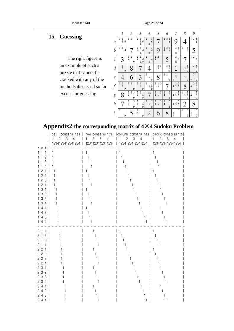
15. Guessing

The right figure is

an example of such a

puzzle that cannot be

cracked with any of the

methods discussed so far

except for guessing.

Appendix2 the corresponding matrix of 4×4 Sudoku Problem

| cell constraints | row constraints |column constraints| block constraints|

| 1 2 3 4 | 1 2 3 4 | 1 2 3 4 | 1 2 3 4 |

| 1234123412341234 | 1234123412341234 | 1234123412341234 | 1234123412341234 |

r c # - - - - - - - - - - - - - - - - - - - - - - - - - - - - - - - - - - - - - - -

1 1 1 | 1 | 1 | 1 | 1 |

1 1 2 | 1 | 1 | 1 | 1 |

1 1 3 | 1 | 1 | 1 | 1 |

1 1 4 | 1 | 1 | 1 | 1 |

1 2 1 | 1 | 1 | 1 | 1 |

1 2 2 | 1 | 1 | 1 | 1 |

1 2 3 | 1 | 1 | 1 | 1 |

1 2 4 | 1 | 1 | 1 | 1 |

1 3 1 | 1 | 1 | 1 | 1 |

1 3 2 | 1 | 1 | 1 | 1 |

1 3 3 | 1 | 1 | 1 | 1 |

1 3 4 | 1 | 1 | 1 | 1 |

1 4 1 | 1 | 1 | 1 | 1 |

1 4 2 | 1 | 1 | 1 | 1 |

1 4 3 | 1 | 1 | 1 | 1 |

1 4 4 | 1 | 1 | 1 | 1 |

- - - - - - - - - - - - - - - - - - - - - - - - - - - - - - - - - - - - - - - - - -

2 1 1 | 1 | 1 | 1 | 1 |

2 1 2 | 1 | 1 | 1 | 1 |

2 1 3 | 1 | 1 | 1 | 1 |

2 1 4 | 1 | 1 | 1 | 1 |

2 2 1 | 1 | 1 | 1 | 1 |

2 2 2 | 1 | 1 | 1 | 1 |

2 2 3 | 1 | 1 | 1 | 1 |

2 2 4 | 1 | 1 | 1 | 1 |

2 3 1 | 1 | 1 | 1 | 1 |

2 3 2 | 1 | 1 | 1 | 1 |

2 3 3 | 1 | 1 | 1 | 1 |

2 3 4 | 1 | 1 | 1 | 1 |

2 4 1 | 1 | 1 | 1 | 1 |

2 4 2 | 1 | 1 | 1 | 1 |

2 4 3 | 1 | 1 | 1 | 1 |

2 4 4 | 1 | 1 | 1 | 1 |


- - - - - - - - - - - - - - - - - - - - - - - - - - - - - - - - - - - - - - - - - -

3 1 1 | 1 | 1 | 1 | 1 |

3 1 2 | 1 | 1 | 1 | 1 |

3 1 3 | 1 | 1 | 1 | 1 |

3 1 4 | 1 | 1 | 1 | 1 |

3 2 1 | 1 | 1 | 1 | 1 |

3 2 2 | 1 | 1 | 1 | 1 |

3 2 3 | 1 | 1 | 1 | 1 |

3 2 4 | 1 | 1 | 1 | 1 |

3 3 1 | 1 | 1 | 1 | 1 |

3 3 2 | 1 | 1 | 1 | 1 |

3 3 3 | 1 | 1 | 1 | 1 |

3 3 4 | 1 | 1 | 1 | 1 |

3 4 1 | 1 | 1 | 1 | 1 |

3 4 2 | 1 | 1 | 1 | 1 |

3 4 3 | 1 | 1 | 1 | 1 |

3 4 4 | 1 | 1 | 1 | 1 |

- - - - - - - - - - - - - - - - - - - - - - - - - - - - - - - - - - - - - - - - - -

4 1 1 | 1 | 1 | 1 | 1 |

4 1 2 | 1 | 1 | 1 | 1 |

4 1 3 | 1 | 1 | 1 | 1 |

4 1 4 | 1 | 1 | 1 | 1 |

4 2 1 | 1 | 1 | 1 | 1 |

4 2 2 | 1 | 1 | 1 | 1 |

4 2 3 | 1 | 1 | 1 | 1 |

4 2 4 | 1 | 1 | 1 | 1 |

4 3 1 | 1 | 1 | 1 | 1 |

4 3 2 | 1 | 1 | 1 | 1 |

4 3 3 | 1 | 1 | 1 | 1 |

4 3 4 | 1 | 1 | 1 | 1 |

4 4 1 | 1 | 1 | 1 | 1 |

4 4 2 | 1 | 1 | 1 | 1 |

4 4 3 | 1 | 1 | 1 | 1 |

4 4 4 | 1 | 1 | 1 | 1 |

- - - - - - - - - - - - - - - - - - - - - - - - - - - - - - - - - - - - - - - - - --


References [1] Herzberg, Agnes M., and M. Ram Russell. 2007

Sudoku Squares and Chromatic Polynomials.

http://www.ams.org/notices/200706/tx070600708p.pdf

[2] Bartlett, Andrew C., and Amy N. Langville. 2006

An Integer Programming Model for the Sudoku Problem

http://www.cofc.edu/~langvillea/Sudoku/sudoku2.pdf

[3] Choudhary, Ashish

Solving Subgraph Isomorphism and Exact Cover by 3-Sets Problem in Linear Time

Using HNEP

http://www.cse.iitk.ac.in/users/iriss05/presentation_a_chaudhary.pdf

[4] Gomes, Carla P., and David B. Shmoys. 2002

The Promise of LP to Boost CSP Techniques for Combinatorial Problems

http://www.emn.fr/xinfo/cpaior/Proceedings/CPAIOR-21.pdf

[5] Gomes, Carla P., and Bart Selman. 2005

Exploiting Heavy-tailed Phenomena in Computation

http://www.cs.cornell.edu/gomes/TALKS/gomes-aaas-2005.pdf

[6] Gomes, Carla P.. 2005

Complete Randomized Backtrack Search Methods: Connections between Heavy-tailed

distributions, Backdoors, and Restart techniques.

http://www.iiia.csic.es/cp2005/hand-tut-gomes.pdf

[7] Yato, Takayuki. 2003

Complexity And Completeness Of Finding Another Solution And Its Application To

Puzzles

http://www-imai.is.s.u-tokyo.ac.jp/~yato/data2/SIGAL87-2.pdf

[8] Davis, Tom. 2007

The Mathematics of Sudoku

http://www.geometer.org/mathcircles/sudoku.pdf

[9] Knuth, Donald E.. 2000

Dancing Links

http://www-cs-staff.stanford.edu/~knuth/preprints.html

[10] Felgenhauer, Bertram, and Frazer Jarvis

~2005. Enumerating possible Sudoku grids

http://www.afjarvis.staff.shef.ac.uk/sudoku/sudoku.pdf.

~2006. Mathematics of Sudoku I

http://www.afjarvis.staff.shef.ac.uk/sudoku/felgenhauer_jarvis_spec1.pdf

[11] Russell, Ed, Frazer Jarvis. 2006


Mathematics of Sudoku II

http://www.afjarvis.staff.shef.ac.uk/sudoku/russell_jarvis_spec2.pdf

[12] Related information on Wikipedia

http://en.wikipedia.org/wiki/Sudoku

Documents

The Application of Exact Cover to the Creating of Sudoku Puzzle