The World Bank INU-55Policy, Planning and Research Staff

Infrastructure and Urban Development Department

Report INU 55

Inflation, Monetary Balances andthe Aggregate Production Function:

The Case of Colombia

by

Robert Buckley and

Anupam Dokeniya

October 1989

DISCUSSION PAPER

This is a document published informally by the World Bank. The views andinterpretations herein are those of the author and should not be attributed tothe World Bank, to its affiliated organizations, or to any individual acting ontheir behalf.

FILE COPY

Pub

lic D

iscl

osur

e A

utho

rized

Pub

lic D

iscl

osur

e A

utho

rized

Pub

lic D

iscl

osur

e A

utho

rized

Pub

lic D

iscl

osur

e A

utho

rized

Copyright 1989 0TIve World Bank1818 H Street, N.W.

ALL Rights ReservedFirst Printing October 1989

This is a document published informally by the World Bank. In order that the information containedin it can be presented with the least possible delay, the typescript has not been prepared in accordance withthe procedures appropriate to formal printed texts, and the World Bank accepts no responsibility for errors.

The World Bank does not accept responsibility for the views expressed herein, which are those of theauthor and should not be attributed to the World Bank or to its affiliated organizations. The findings,interpretations, and conclusions are the results of research supported by the Bank; they do not necessarilyrepresent official policy of the Bank. The designations employed, the presentation of material, and any mapsused in this document are solely for the convenience of the reader and do not imply the expression of anyopinion whatsoever on the part of the World Bank or its affiliates concerning the Legal status of any country,territory, city, area, or of its authorities, or concerning the delimitations of its boundaries or nationalaffiliation.

The authors are Robert Buckley, Sr. Economist, and Anupam Dokeniya, Researcher, Infrastructure andUrban Development Department, The World Bank. Helpful comments were made by WiLLiam Easterly, Emmanuel Jimenez,Kyu Sik Lee, Desmond McCarthy, Jacques Polak, Bertrand Renaud and Alan Walters. They, of course, are notresponsible for any remaining errors. The views expressed are not those of The World Bank.

The World Bank

Inflation, Monetary Balances andthe Aggregate Production Function:

The Case of Colombia

DISCUSSION PAPER

ABSTRACT

The role of monetary balances in economic growth has long been a topicof macroeconomic research. Following the work of Sinai and Stokes (1972), a

number of studies have given this perspective empirical content. By

demonstrating the significance of the role of monetary balances in an aggregate

production function, this work has shown that money and financial policy need

to be carefully considered in studies of growth.

This paper also examines the role of real money balances in anaggregate production function of a developing economy, Colombia. In addition

to being a developing country, Colombia is also interesting to analyze in this

way for a number of other reasons. First, although it has experienced high andvariable rates of inflation, it has also introduced a competitive system ofquasi-monetary balances that have been indexed for inflation. In fact, thesuccess of this system appears to have played a significant role in the continuedexpansion of the Colombian financial system.

Second, as one of the most extensively studied developing countries

in the world, data on Colombia are more readily available than they are for otherdeveloping countries. In this respect, Colombia is one of the few developing

countries for which an empirical study of the effects of financial policy oneconomic growth can be made. There is little empirical work on this topic, andColombia represents an unusual opportunity to perform such analysis.

Finally, the role that monetary balances may have played in economic

growth in Colombia is of interest because indexed mortgages played a major rolein this change in financial policy. Rather than deregulating the interest rate

on deposits and thereby simply permitting a more competitive market for

broadly-defined monetary balances, Colombia induced more competition. It didthis by introducing indexed mortgages which provided higher yields on depositsthan those available at commercial banks. In a sense, these indexed mortgages

were similar to introducing a competitive "Trojan Horse" into the Colombianfinancial system. Other depository institutions had to compete with indexed

mortgage lenders for deposits. Our results indicate that it was not the effects

of finance on the composition of investment patterns that mattered. Rather,growth was stimulated by not only permitting but by inducing the financial systemto be able to minimize the effects of high and variable inflation rates on the

cost of monetary balances. Household access to credit for "low priority"

investments played an important part in the process of inducing a cost-reducing,more competitive financial technology. While it does not appear that the forced

investment schemes that still litter the financial system have made the best use

of the resources mobilized by the more competitive deposit system, one can only

speculate about what would have occurred if the resources were not in the

financial system at all.

INFLATION, MONETARY BALANCES ANDTHE AGGREGATE PRODUCTION FUNCTION

THE CASE OF COLOMBIA

Table of Contents

Page No.

I. INTRODUCTION................. .... . . . . 1

II. INDEXED MONETARY BALANCES IN COLOMBIA. ........ . . . . 4

III. THE MODEL AND THE DATA............. .... . .. 10

IV. THE AUGMENTED PRODUCTION FUNCTIONAND OTHER STUDIES OF COLOMBIAN ECONOMIC GROWTH.... . . . .. 14

A. Indexation and Economic Growth.... .... . . . .. 14

B. Income Distribution Issues........ ... . . .. 15

C. Financial Policy and the Sources of Growth.... . . .. 16

V. CONCLUSION.................... . . . . .. 18

APPENDIX I . . . . . . . . . . . . . . . . . . . . . . . . . 20APPENDIX II . . . . . . . . . . . . . . . . . . . . . . . . . 21

TABLES

Table 1 - Behavior of Monetary Aggregates and Inflation

over the 1958-84 Period . . . 8Table 2 - Estimates of the Parameters of the Cobb-Douglas

Production Function, with and without Real Money

Balances, Corrected for Autocorrelation, for the

years 1958-1984........ ..... . . . . 22Table 3 - Estimates of the Parameters of the Cobb-Douglas

Production Function, with Real Money Balances

(with and without Adjustment for Indexation and

Inflation) Corrected for Autocorrelation, for

the Years 1958-1984......... ... . .. 23

- 111 -

Page No.

TABLES (continued)

Table 4 - Estimates of the Parameters of the Cobb-Douglas

Production Function, with the without Real Money

Balances, Corrected for Autocorrelation, for the

Years 1958-1984. (Capital is Adjusted for CapacityUtilization and Labor is Adjusted for Change in Sex

Composition and Education). ......... . ..24Table 5 - Data for Colombia 1958-1984....... . . . . . .. 25Table 6 - Natural Logarithmic Transformation of the Variables . 26

Table 7 - GDP of Colombia 1958-1984. . .......... . ..27Table 8 - Capital Stock for Colombia 1958-1984..... . . ..28Table 9 - Labor Force in Colombia 1958-1984..... . . . . ..29Table 10 - Monetary Balances in Colombia 1958-1984..... . ..30Table 11 - Real Monetary Balances for Colombia 1958-1984 . . . 31

Table 12 - Indexed Real Money Balances for Colombia 1958-1984 32

Table 13 - Regression with No Money Variable..... . . . . .. 33

Table 14 - Data Used for Using Solow's Approach to Find

Components of Growth........ ..... .. 34

Table 15 - Data Used for Predicting the Values...... . . .. 36

Table 16 - Ratio of M2 (Broadly Defined Money) Over GDP . . . 37

Table 17 - Regression Results of Financial Deepening Over Time 38

Table 18 - Inflation Tax on Money Balances as a Share of Income. 39

FIGURE

Figure 1 - Inflation Tax on Monetary Balances as a Share ofIncome . . . . . . . . . . . . . . . . . . . . . . 40

BIBLIOGRAPHY................ .... . . . ..41

INFLATION, MONETARY BALANCES ANDTHE AGGREGATE PRODUCTION FUNCTION

THE CASE OF COLOMBIA

I. INTRODUCTION

1.01 The role of monetary balances in economic growth has long been a topicof macroeconomic research, see, among others, Levhari and Patinkin (1968).Following the work of Sinai and Stokes (1972), a number of studies have giventhis perspective empirical content. By demonstrating the significance of therole of monetary balances in an aggregate production function, this work hasshown that money and financial policy need to be carefully considered in studiesof growth. More recently this type of empirical analysis has been extended tothe production function of a developing country, Pakistan, by Khan and Ahmad(1985). Their results are consistent with the findings for the U.S. and Japan--that is, real money balances are an important factor of production.

1.02 This paper also examines the role of real money balances in anaggregate production function of a developing economy, Colombia. In addition tobeing a developing country, Colombia is also interesting to analyze in this wayfor a number of other reasons. First, although it has experienced high andvariable rates of inflation, it has also introduced a competitive system ofquasi-monetary balances that have been indexed for inflation. In fact, thesuccess of this system appears to have played a significant role in the continuedexpansion of the Colombian financial system. See the World Bank (1987), andBarro (1975).

1.03 Over the 1974 to 1984 period, for example, Colombia was one of the fewLatin American countries not to experience any significant reduction in broadlydefined monetary assets as a share of GDP.1 1 In contrast to most other LatinAmerican countries, Colombian monetary balances continued to grow more rapidlythan did the economy without any significant interruptions. It would beinteresting to determine whether this more competitive and buoyant financialsystem reduced the costs of this factor of production by such an extent that itaffected the level of economic growth.

1/ Data on M2\GDP for Argentina, Brazil, Chile, Colombia, Mexico, and Peru forthe 1974-84 period indicate that all of these countries except Colombia at leastonce experienced a substantial reduction in broadly-defined monetary balancesas a share of GDP. The Colombian ratio was much less volatile, as well as almostmonotonically increasing. In one year, 1979, there was a less than one percentdecrease in M2/GDP. A log linear regression of M2/GDP-Aeu', where t-time, foreach of the six countries for the 1974-84 period (Mexico only 1977-84) indicatesthat in Colombia the coefficient on time was positive and significant at the onepercent level, and the R2 was equal to .68. The results for the other countriesdid not yield a significant time trend except for Brazil, but in Brazilian case,the coefficient was negative. Source for the data is International FinancialStatistics.

-2-

1.04 Second, as one of the most extensively studied developing countriesin the world, data on Colombia are more readily available than they are for otherdeveloping countries. Indeed, this empirical analysis can be undertaken onlybecause the time series data from two other studies, by Harberger (1969) and aPresidential Employment Study as reported in World Bank (1987) were developed,and in the former case updated. In this respect, Colombia is one of the fewdeveloping countries for which an empirical study of the effects of financialpolicy on economic growth can be made. As Fry (1988) shows, there is littleempirical work on this topic, and Colombia represents an unusual opportunity toperform such analysis.

1.05 Third, work on the sources of growth in Colombia, by Elias (1978),Hanson et. al. (1985), indicates that one of the larger "unexplained" sourcesof growth in Colombia over the 1960-1980 period occurred during the period whenfinancial sector policy innovations were introduced. Once again, it would beinteresting to determine whether this higher level of technical change can beempirically related to the financial innovations.

1.06 Finally, the role that monetary balances may have played in economicgrowth in Colombia is of interest because indexed mortgages played a major rolein this change in financial policy. Rather than deregulating the interest rateon deposits and thereby simply permitting a more competitive market forbroadly-defined monetary balances, Colombia induced more competition. It didthis by introducing indexed mortgages which provided higher yields on depositsthan those available at commercial banks. In a sense, these indexed mortgageswere similar to introducing a competitive "Trojan Horse" into the Colombianfinancial system. Other depository institutions had to compete with indexedmortgage lenders for deposits. The central way that they could do this wasthrough paying more competitive interest rates on financial instruments. Overthe 1972-84 period, for example, commercial bank certificates of deposit had anex post average real return of 2.5 percent, after having yielded an averagenegative 6.5 percent real return for the previous 14 years. 1

1.07 This kind of increased competition for funds may have a number ofdesirable allocative effects. However, it could also cause mortgage borrowersto "crowd out" other investments, as suggested by Carrizosa et. al. (1982). Inmany developing countries financial regulators proscribe the supplying ofmortgages by the formal financial system because of this latter concern. Inthis respect, the study is one of the first attempts to analyze empirically thepossible macroeconomic effects of providing households access to mortgage creditat competitive interest rates.

1.08 Coherent with the preliminary nature of our research, the econometricspecification of the study is similar to the original Sinai and Stokes approach.

2/ The rate of return over the 1958-71 period are ex post rates inferred fromCarrizosa et. al. (1982); the data for the later period are from Correa (1986).Berry and Urrutia (1976) also provide data on real deposit rates and a discussionof the broader effects of mortgage lending policies in the pre-indexation period.

- 3 -

Indeed, the approach taken is very much in the spirit of the original Solow(1957) article on aggregate production functions and the sources of growth. Thatis, we hope that we are not pushing the data beyond what can reasonably beinferred from such aggregate measures. Nevertheless, despite the more heuristicthan strictly quantitative nature of the analysis, we think that our resultsprovide robust if imprecise evidence that a more competitive deposit and creditmarket played an important role in Colombia's economic growth.

1.09 The plan of the paper is as follows. The next section reviews theeffect that inflation can have on the cost of monetary balances and the way thatindexation affects these costs. Then, the Colombian experience with inflation,indexation, and increased financial competition is described. The effects ofinflation on monetary aggregates and what we term "equivalent units" of thisfactor of production are examined and compared to the levels that would havebeen obtained in the absence of indexation. In Section III the data andempirical results are presented and discussed. Section IV reviews previousanalyses of Colombian economic growth in light of the findings, and discussesthe policy implications of our findings. A final section summarizes.

II. INDEXED MONETARY BALANCES IN COLOMBIA

2.01 For households, the transaction costs of expenditures can be minimizedif transaction balances can be placed into highly liquid deposits that are not

affected by changes in the inflation rate. For the most part, the savings andtime deposits offered by the Colombian Caja Ahorra de Vivienda (CAVs), savings

and housing corporations, have been such instruments. While in recent years

ceilings on the amount of adjustment for inflation have reduced the real returnon these deposits, the record of their largely positive ex post return since 1972has built confidence in the use of such instruments.

2.02 The CAVs were created in 1972 by a series of decrees by the Pastranagovernment. The government relied upon Constitutional authority relating to thedisposition of personal savings and their development played a major role in thegovernment's development strategy.1 1 Their design and implementation were placedunder the direction of Laughlin Currie.Al These institutions were introducedinto a financial system which had allocated a contracting share of nationalresources to the formal financial sector and which operated parallel to athriving and growing informal sector. For example, over the 1965-69 periodcredit outstanding as a share of GDP averaged 15 percent, whereas it averaged

19 percent in the preceding five year period. In contrast, by the 1980-84period, the net credit outstanding as a share of GDP averaged 36 percent, andthere is indirect evidence that the level of economic activity in the informal

sector had secularly contracted.5'

2/ See Berry and Soligo (1980) for a discussion of the development strategyand Sandilands (1980) for a discussion of the CAVs creation and their earlyregulation.

/ Currie was formerly the chief advisor to both Mariner Eccles, Chairman of

the Federal Reserve Board, and President Roosevelt. He also directed the firstWorld Bank mission to Colombia in 1949.

./ The informal sector generally has three important dimensions: finance,employment and housing production. In contrast to many other Latin American

economies, each of these aspects of the informal sector appeared to contractduring the 1970s. See the World Bank (1987), p. 70 for further discussion ofthe expansion of the formal financial sector in the 1970s mentioned in the text.With respect to housing, Urrutia (1985) p. 64 documents the very significantformalization of the housing stock that took place over the 1970s. The World

Bank (1983) p.1 9 -2 3 provides a discussion of labor participation over the 1960sand 1970s saying that in the latter period the employment expansion would appearto be the highest achieved by a big country over a comparable period. After

1972 employment in the informal sector continued to grow more rapidly than did

employment in the formal sector. However, it grew at a less rapid rate than in

the 1958-72 period even though total employment expanded much more rapidly inthe second period. Over the period 1958-72 the share of the labor force in theinformal sector showed an increasing trend, expanding in all the years except

- 5 -

2.03 As financial intermediaries, the CAVs represented both a liberalizationand a further specialization of an already highly segmented and controlledfinancial system. They were a liberalization because they financed mortgagesat positive ex ante real interest rates that were initially fully indexed forinflation, and they paid their depositors a similarly indexed real return.However, because they were the only intermediaries allowed to index both theircredit and their liabilities to a unit of constant purchasing power, calledUPACs, they were also a further specialization of the financial system. Thisspecialization increased over time through a series of regulations that governedthe share of the CAV portfolio that had to be lent for certain loan sizes, theinterest rate that could be charged, and the permissible loan-to-value ratioof the various loan amounts, among other directives that were designed to insurethat CAV lending was targeted towards lower and moderate-income borrowers.&

2.04 The return on CAV deposits was originally based on a three month movingaverage, for the months immediately preceding the calculation, of the combinedconsumer price indices of blue and white collar workers. Currently, the indexis still changed daily with the quotations for the next month announced inadvance. This method of indexation of the return on deposits of course meansthat the index is based on the past rate of inflation rather than a measure ofinflation during the holding period for the deposit. It implies that anindividual who deposits funds in a CAV knows with certainty the nominal rate ofreturn but not the real rate of return. Consequently, the central feature ofindexation is not that the financial contract has immunized real returns fromthe effects of inflation. Rather, the chief features have been to create asystem of deposits on which the interest rates gradually adjust to changes inthe rate of inflation and provide a competitive real return to savers.

2.05 Such a system is hardly the idealized method of indexation that isrecommended by economists. See Fischer (1975). Nevertheless, these financialinstruments have provided a means to avoid most of the inflation tax on short-term financial assets and transaction balances, and as Barro (1975) says they"have induced some increases in the nominal interest rates paid on otherfinancial assets,.." p.5. They have, in other words, lowered the costs ofrelying on the formal financial sector to provide a service that a formal sectorinstitution should have a comparative advantage in providing.

2.06 An approximation of how Colombian policy reduced the effects ofinflation on the costs of holding monetary balances can be made by computing ameasure of the aggregate tax rate on monetary balances. Prior to theintroduction of indexation, this tax applied to all monetary balances becausenominal interest rates on time deposit were both largely invariant with respect

in three, when the decrease was negligible. In the 1972-86 period, in contrast,the informal market share contracted in half the years even though the indirectcosts of formal sector employment increased sharply.

A/ See Isaza (1987) for a complete listing of all the regulations governingCAVs since their creation, and Carrizosa et. al. (1982) for a discussion ofbroader financial market policies that have affected the functioning of the CAVs.

- 6 -

to changes in the inflation rate and lower than the inflation rate.2 1 As aconsequence, increases in the inflation rate affected the cost of Ml, currencyand demand deposits, as well as M2, which also includes time deposits. The taxon M1 is straightforward and in steady state is equal to 8(1+0), where 8 is theinflation rate.

2.07 For time deposits, prior to the introduction of CAVs, the tax is morecomplicated. Because longer term deposits yielded a negative real rate ofreturn, the income to these assets was taxed at a 100 percent rate. But inaddition, because the nominal return on these deposits, Rn, was always less thanthe inflation rate, these assets also lost value over time. Bringing all theseeffects together, the tax rate on what might be termed equivalent units ofmonetary balances can be described by

1)Ti- Ml (e - Rn) (M2 - Ml) (M2 - Ml)(1 + e) x-Y (1 + (6-Rn)) Y Y

Rr is the real return on time deposits, and Y is GNP. The first and secondterms on the right hand side express the tax on monetary balances as the shareof income that would be needed to restore these balances to their prior level.In other words, they represent taxes on the stock of M1 and (M2-M1) balances,respectively. The tax on real return on the non-M1 portion of the monetarybalances is represented by the third term on the right hand side.

2.08 Now consider how the introduction of indexed time and savings depositsaffects this tax.!! If the return on time deposits competes with the return onCAV time deposits, and this real return becomes invariant with respect to changesin the inflation rate inflation would apply only to Ml, and not at all to M2 orM3, which includes M2 plus CAV deposits. In this case the tax rate on monetarybalances like Bailey's (1956) stylized descriptions of the inflation tax is:

(2) T2 - Mi(1 + e) Y

This kind of regulatory change eliminates both the inflation tax and loss ofreal return on non-Mi monetary balances, and it results in the inflation taxbeing applied only to M1 balances. It amounts to assuming that the cost of theindexed balances is unaffected by changes in the inflation rate, so that non-Mimonetary balances become superneutral.

7./ See Carrizosa et al. (1982).

3/ Strictly speaking, the indexed time and savings deposits (CAV's) should bepart of M2, but in our analysis, we separated the CAV deposits from M2 to isolatethe effects of these deposits. The treatment, as far as taxes are concerned,of these two "monies" (M2-Ml) and (M3-M2) are identical from 1973 onwards.

- 7 -

2.09 However, besides making the real rather than the nominal return ontime deposits less variable with respect to changes in the inflation rate, theintroduction of the CAVs also blurred the distinctions between the types ofmonetary balances. For example, Montenegro and Garcia (1986) found that afterthe introduction of indexation, the velocity of currency secularly increased.The continual decline in the share of Ml held in currency (from 31 percent in1960 to less than 24 percent in 1974) was reversed. By 1984 the share of Mlheld in currency had once again reached the level of 1960. They also found thatthe holdings of currency plus CAV savings deposits was without trend. Theysuggest that this latter result implies that CAV saving deposits became closesubstitutes for currency. In effect, CAV deposits became another vehicle throughwhich the inflation tax could be avoided and the costs of holding monetarybalances reduced.

2.10 Figure 1 plots out the tax rate on the monetary balances as a shareof income described by the above equations. It also traces out the inflationrate. Prior to 1973, TI is used to measure the tax rate and after that T2 isthe tax rate. It is quite clear that the inflation tax relative to inflationrate was very significantly reduced. 2 1 The tax rate per percent of inflation is0.166 percent in the former period and 0.116 percent in the latter period.1 1Some evidence of how this reduction in the inflation tax rate and increase in

the inflation rate affected the holdings of monetary balances is presented inthe following table.

9/ The estimates are stylized for a number of reasons. Most importantly theyuse ex post measures of inflation rather than the ex ante rates that motivatethe holdings of various types of balances. In addition, the assumption that realreturns become completely invariant with respect to the inflation rate afterindexation was introduced is an exaggeration. Complete insulation of realreturns was not achieved so that assumption lowers the estimated tax rate. Onthe other hand, however, we make no attempt to account for the blurring ofdistinctions between types of monies. This assumption causes the estimates oftax in the post-1972 period to err in the other direction. Finally, we assumethat the real rate of interest was constant and equal to 2.5 percent throughoutthe period.

10/ These numbers were obtained by calculating average inflation rates andaverage inflation tax over the two time periods; 1958-1972 and 1973-1984. Forthe time period 1958-1972, Ti was the inflation tax used and for 1973-84 period,T2 was the inflation tax used. The average inflation tax was divided by theaverage inflation rate to get these numbers.

- 8 -

Table 1: BEHAVIOR OF MONETARY AGGREGATES AND INFLATIONOVER THE 1958-84 PERIOD

1958-72 1973-84

Ml/GDP > 0 < 0

M/GDP 0 > 0

M1/M .85 .57

M1/M > 0 < 0

E .110 .235

The . indicates a derivative with respect to time.

In the latter period, the coefficients were of an

opposite sign from the former period and the standard

errors were greatly reduced.

2.11 In the pre-indexation period broadly-defined monetary balances, M,was a relatively constant share of GDP. In addition, Ml share of total monetarybalances showed an increasing trend. In the latter period, behavior was very

different: M1 declined in importance (as a share of both GDP and M), as firms

and households avoided the tax of the latter period's higher inflation rate.At the same time, broadly-defined monetary balances increased, as the return on

these balances were better insulated from changes in the inflation rate.

2.12 To summarize, with the introduction of indexation, the Colombianfinancial system became competitive on the resource mobilization side. This

competition for funds provided a way for households and firms to avoid much of

the increase in the inflation tax on transaction balances that would haveoccurred as a result of the sharp increase in the inflation rate. On the otherhand, this system can hardly be described as a liberalized system thatcompetitively allocates resources. As Correa (1986) documents, the assets of

the system are still targeted to a wide range of below market interest rate loansin agriculture, industry, and low-income housing.

11 /

2.13 A financial system that encourages more competition for deposits and

simultaneously requires lenders to make below market rate loans ultimatelyimposes the costs of the loans on the institutions rather than the depositors.

Ll/ Indeed, recent work by Dailami (1989) suggests that Colombian corporationsare making use of below market interest rate credit to buy market rate financialassets. His work shows that in 1983 financial assets accounted for 20 percent

of total assets of non-financial corporations in Colombia. This figure is doublethe rate observed in developed economies.

- 9 -

Hence the financial crisis that has affected the commercial banking system sincethe end of 1982 is not surprising.! 1 But, this crisis is not the result of theincreased competitiveness of the financial system. Rather, it is theincompleteness of the deregulation- -particularly the restrictions on lendersasset powers--that has created the problems.

12/ See World Bank (1987) and (1983) for discussions of the financial stressin Colombia. In 1982 this stress lead to a financial crisis and the creationof Fund to Guarantee Financial Institutions. The former study suggests thatsince 1985, after our estimation period, the structural weaknesses of thefinancial system became pronounced, p. 72.

- 10 -

III. THE MODEL AND THE DATA

3.01 A simple Cobb-Douglas production function with nonconstant returns toscale is assumed and estimated in log-linear form. Like Sinai and Stokes, werely on single equation OLS estimation, corrected where necessary forautocorrelation. Our rationale for this single equation specification is twofold:first, the exploratory nature of our work; and second, the research subsequent

to Sinai and Stokes' first article suggests that FIML, simultaneous equationsor 2SLS approaches do not result in significant changes in the estimatedcoefficients in any of the countries for which the functions have been estimated.See, for example, Sinai and Stokes (1977), and (1981), as well as Short (1979),and Khan and Ahmad (1985). Cumulatively, the work that has followed the originalarticle suggests that OLS estimation is a reasonable approach. While weacknowledge the potentially substantial problems that could arise from

simultaneity concerns, they are not dealt with here.131

3.02 The following equation was estimated with annual data over the 1958-

84 period.

(3) In GDP = In A + a In K + B In L + yln M + u

where,

GDP - total output,K - capital,L - labor,M - equivalent units of real money balances.

A = an efficiency parameter, and the Greek letters are estimatedparameters and u is a disturbance term.

3.03 Data for output, labor, and capital were taken from a number of recentWorld Bank studies of the Colombian economy. Data on real output and the real

capital stock were obtained from an update of a Harberger (1969) study of the

Colombian capital stock. Data on real monetary balances are from the Banco de

la Republica as reported in various World Bank documents. Employment data are

from a Presidential Employment Mission, as reported in the World Bank (1987).They measure the number of persons in the labor force. This measure is a poorer

11/ Romer (1987) raises doubts as to whether problems of simultaneity can be

overcome by instrumental variables. He says "there is little hope that valid

instruments exist." p. 186.

- 11 -

measure of actual labor input than is hours worked but, as Romer (1987)indicates, it is at least symmetric with the measure of capital input.-1

3.04 Our measure of equivalent units of monetary balances modifies theSinai and Stokes' approach to account for the effects described in equations (1)and (2). To adjust for the more competitive yields on post-indexation timedeposits, we assume that prior to indexation all monetary balances were taxedat the inflation rate, which is measured by the GDP deflator, and that afterindexation was introduced in 1972, this tax applied only to Ml. That is, afterindexation was introduced time deposits yielded the market rate of interest andhence did not bear any inflation tax; and prior to the introduction of indexationboth the Ml and (M2-Ml) components of monetary balances were subject to theinflation tax as described in equation(1). 1 See the appendix for a completedescription of all the variables.

3.05 Table 2 presents the results of the estimated equations with andwithout monetary balances. Equation (4) in the table indicates that a standardCobb-Douglas production function without monetary balances describes theColombian data fairly well. The returns to scale, 1.4, and the outputelasticities -- labor 68 percent and capital 51 percent -- are similar to the

results of Khan and Ahmad (1985) for Pakistan. They found returns to scale of1.33 without money balances and elasticities of 75 and 58 percent, respectively.Sinai and Stokes (1972) also reported increasing returns to scale for the U.S.,1.78. Although their output elasticities, (1.36 and .43 respectively) were verydifferent from ours, these kinds of differences between developed and developingcountries--in particular a much higher relative elasticity for capital in

14/ We also estimated equations which adjusted the labor input for the effectsthat female participation rates and education would have in a manner suggestedby Hanson et. al. (1985). Similarly, we also constructed measures of theutilized capital stock by relying on Cuddington's (1986) measures of permanentand cyclical measures of real GDP. We assumed that the capital stock wascompletely utilized in 1974, the year in which Cuddington estimates GDP was atthe highest cyclical peak of our estimation period. In other years capital wasassumed to be less than fully utilized by the same percent that cyclical outputwas less than output in the peak year. Equations estimated with theseadjustments reduced the standard error of the equations and the regressioncoefficients. These results are not reported because of concern with ad hoc datatransformations in an already highly aggregated equation. The results areavailable upon request.

1/ To give a concrete example of our adjustment for equivalent units ofmonetary balances, suppose that in real terms 100 units of M are observed in bothperiods 1 and 2, and that the inflation rate was 5 percent higher in period 2.In this case the holder of monetary balances in period 2 would have to allocatemore of his income to such balances to derive the same level of services. Justas the Darby effect indicates that nominal interest rates must increase by1/1-T to keep real returns constant with respect to a change in the rate ofinflation, our approach implies that equivalent units of monetary balances aresimilarly constant if they are adjusted by 1/1-T where T=-.

- 12 -

developing economies--are consistent with Elias's (1978) findings for LatinAmerica.

3.06 All but one of the coefficients in equations 4-7 are significant atthe five percent level, (the labor coefficient in equation 5 is significant atthe 10 percent level). The standard error of equation (4) without correctionfor autocorrelation, .047, is larger than the Sinai and Stokes estimate (.034)for a much longer period with superior input measures for the U.S. Equations5-7 show that whether defined as Ml, M2, or M3, real monetary balances are ofsubstantial importance when added to this standard production function. Thestandard error of the equation uncorrected for autocorrelation is reduced inevery case; to .021 for the equation including Ml, .032 for the equationincluding M2, and .04 for the equation with M3. In addition, estimates ofequations that were not corrected for autocorrelation indicate that there ismuch less of a problem in this regard in equations 5-7, than there is in equation4, as would be expected if monetary balances were an omitted variable in equation

3.07 The coefficients on our measures of monetary balances ranged from .23to .37. These results are somewhat higher than those of Sinai and Stoke's, .17to .21, and somewhat lower than Khan and Ahmad's for Ml, .43 . Adding Ml to theequation did not significantly affect the returns to scale, whereas adding M2or M3 did. The latter variables also reduced the contribution of labor by a muchgreater amount as is the case in previous research. Similarly, the pattern ofchange in coefficients when monetary balances are added to the estimated functionis qualitatively similar to those of Sinai and Stokes. In particular:

a5 < a4 and a6 Z a7 > a5; and B6 =7 5 =4 where the subscripts

indicate the nun-'er of the equation.

3.08 Table 3 compares estimates of equation (3) without adjustment ofmonetary balances (M2) for equivalent units, i.e., like those of Sinai and Stokeswith our adjusted measure of M2 from Table 2. A comparison of the resultsindicates that the adjustment to account for the inflation taxes on monetarybalances improves the explanatory power of our estimation without having mucheffect on the coefficients of labor or capital. The SEE is lower in the equation

16/ Like Khan and Ahmad (1985), we also estimated equations including a timetrend as a representation of neutral technological progress. Our results weresimilar to theirs. The coefficients of the other variables in the equation werenot significantly different from zero. They suggest that this result seems tobe caused by high collinearity. We also used a non-linear test for theappropriateness of the Cobb-Douglas specification as opposed to a CES functionalform. Our results also provided strong support for the Cobb-Douglasspecification.

- 13 -

where equivalent units of M2 are used and the coefficients are betterconfirmed.1U

3.09 To summarize, like previous studies our estimates suggest that monetarybalances have played an important role in Colombian economic growth and shouldtherefore be included in analyses of the sources of growth. We realize that ourinput data are clearly far from perfect, and even our measure of effect of thechanges in the tax structure in the measurement of monetary balances will notachieve Jorgenson and Griliches' (1967) aspiration of eliminating the residualthrough better measurement of the inputs. Nevertheless, the robustness of ourestimates under various input definitions is at least suggestive that ourfindings are not adventitious. Solow's (1988) recent comment on almost exactlythis topic helps put our results in perspective:

"Thus technology remains the dominant engine of growth, with humancapital second. One does not have to believe in the accuracy of thesenumbers; the message they transmit is pretty clear anyway."

"That is meant as a serious remark, every piece of empiricaleconomics rests on a substructure of background assumptionsthat are probably not quite true. Under those circumstances,robustness should be the supreme economic virtue; ... so I

would be happy if you were to accept the results I have beenquoting to point to a qualitative truth and perhaps givesome guide to orders of magnitude." Nobel address (1988)p. 314.

17/ For simplicity the only comparison presented in Table 2 is for equationsthat contain M2. This comparison is the most favorable for the unadjustedmonetary balances. For example, using the unadjusted measure of M3 produces astatistically insignificant coefficient on M3 and a standard error that istrivially smaller, .045 versus .047, than that of the production function withoutmonetary balances, i.e., equation (4). Similar results were obtained in theequation that used an unadjusted measure of M1.

- 14 -

IV. THE AUGMENTED PRODUCTION FUNCTION AND OTHER STUDIES

OF COLOMBIAN ECONOMIC GROWTH

4.01 We focus on three of the many issues that have been raised in theextensive literature on Colombian growth: (1) Has the introduction of indexed

mortgage instruments affected economic growth? (2) Can we draw any conclusions

about the effect of financial policy on income distribution? and (3) Are thereany additional potential "sources of growth" type problems that can beidentified by the inclusion of monetary balances as a factor of production?

A. Indexation and Economic Growth

4.02 Carrizosa et. al (1982) have argued that the introduction of

indexation had little effect on the level of economic growth. They suggest thatbecause of credit fungibility, the central effect of increasing formal sector

mortgage financing was a substitution of financing from alternative sources of

funds. This point of view has been contended by Currie and Rosas (1986) who

argue that mortgage indexation played an important part in Colombia's economic

growth by stimulating housing as a lead sector in the economy.

4.03 Whether mortgage indexation lead to an increased growth rate,particularly in the manner described by Currie (1974) is perhaps an intractableeconometric question. Although the lower average level of GDP invested inhousing after the introduction of indexation does provide some support to the

credit fungibility argument raised by Carrizosa et. al. Our analysis suggests

a different channel through which the introduction of mortgage indexation might

have indirectly affected growth: by stimulating the competition for financial

resources they helped reduce the burden of inflationary taxes on monetarybalances. This effect, in turn, led to a reduction in the costs of an importantfactor of production. According to this perspective, this cost reductionfacilitated investment rather than affected its composition, and therebyaffected growth.

4.04 To get an approximation of the effects of financial technology onoverall growth, it is convenient to assume that the production function islinearly homogeneous, and that the necessary conditions for producer equilibriumapply. With these assumptions output elasticities sum to one, and the effect

of the estimated increasing returns to scale on total factor productivity iseliminated. Comparing the adjusted coefficients from linearized versions ofequations (4) and (6), i.e., production functions with and without monetarybalances, we find that in equation (4) technical change or, in Abramovitz'sterms, the measure of our ignorance, accounts for 72 percent of growth in total

factor productivity. In equation (6), in contrast, technical change accounts

- 15 -

for only 35 percent of the growth in total factor productivity.Il- The inclusionof monetary balances has cut the unexplained residual in half. Hence, even ifour coefficients are off by a factor of two, it appears inescapable that thechange in the structure of financial technology has made a very substantialcontribution to economic growth in Colombia.

B. Income Distribution Issues

4.05 Measuring the incidence of lower inflationary taxes or a morecompetitive financial system is, as Urrutia (1985) shows, a very difficulttask, and our aggregate results shed little direct light on this importantissue. Rather than trying to tease out the possible effects that financialpolicy may have had on income or wealth distribution, as Berry and Soligo (1980)have creatively done, it is perhaps of more interest to consider briefly in thewords of Sherlock Holmes, "a dog that did not bark." The dog in this case isthe observation that the share of income of the lowest income group did notdeteriorate over the 1958-84 period. In fact, it improved. 11 The improvementis surprising because the traditional view of the development process is thatduring development there is generally an initial deterioration in the earningsof lower income groups. Chenery and Syrquin's (1975) model allows for a roughquantification of how income level shares might be expected to behave.LY Itindicates that based on Colombia's income level and population growth over this

1./ The growth in output per unit of labor is decomposed into growth in capitalper unit of labor, growth in monetary balances per unit of labor and theremainder is attributed to "technical change." When monetary balances are notincluded, growth due to capital per labor is 28 percent and technical change,72 percent. However, when monetary balances are included, growth due to capitalis 21.5 percent, technical change, 35 percent and monetary balances, 43.5percent. For more detail, see Solow (1957).

19/ See Reyes (1987) for the most recent data on income distribution. Urrutia(1985) provides the most comprehensive evidence for the 1970s.

20/ The Chenery and Syrquin work is a regression model of the behavior of 101countries over the 1950-1970 period. It "explains" various characteristics ofan economy, e.g. employment in different sectors, urbanization, saving, andincome distribution measures as a function of the level of per capita income andpopulation. The basic perspective of the work is that development processes aresufficiently uniform among countries to produce a consistent pattern of change.The analysis provides measures for the behavior of a representative developingcountry. For Colombia, the model's predictions for employment distribution amongprimary, manufacturing and service sectors were very close to the observedvalues; so too were its estimate of savings and investment rates and thedistribution of income.

- 16 -

period, that a slight deterioration in the share of income in the lowest twoquintals was to be expected.2 11

4.06 The interesting aspect of the somewhat surprising improvement in therelative position of the poor is that one of the chief reasons for proscribingmarket-rate housing finance systems in developing countries is the concern thatthese systems will not only not serve the poor, but they will also lead to adeterioration in the position of the poor. See, for example, Shelter, (1980),The World Bank. Indeed, in many countries the reliance on the housing financesystem to provide "affordable," i.e., very low nominal interest rates, is adirect result of distributional considerations prompted by concerns about thepresumed unaffordability of market-rate mortgage credit. Indeed, the ceilingimposed on the amount that mortgage payments can be adjusted for inflation inColombia is a good example of such a policy.

4.07 We are not suggesting that mortgage indexation was a cause of observeddistributional results. Factors other than housing finance policy or financialpolicy clearly have more to do with the observed trends in income distribution.Nevertheless, the Colombian case is interesting in that it suggests that thedevelopment of market-oriented housing finance systems can make a significantcontribution to economic growth contemporaneously with an improvement in theposition of the lowest income groups. Hence, it does not appear that greateraccess to mortgage credit by moderate and upper income households isantithetical to the interests of the poor.

C. Financial Policy and the Sources of Growth

4.08 Perhaps the most appropriate standard against which to evaluate theusefulness of including monetary balances in the production function is whetherit yields any insights about the sources of growth not suggested by thetraditional growth accounting perspective. The augmented production functionperforms well on this score. The inclusion of monetary balances suggests animportant channel through which macroeconomic financial policy can affectgrowth: the channel is the affect of the level of inflation on thecompetitiveness of the resource mobilization process.

4.09 Since 1984, the last year of our estimation period, the interest ratecap on the mortgage indexation adjustment has been below the rate of inflation.As a result, since that time the mortgages supplied--which now account for 25percent of financial assets--provide lenders no protection against increases inthe inflation rate. If inflation increases, lenders will be unable to increaseborrowers' repayment by as much. Hence these instruments will not provide theCAVs a means of competing for deposits. As a result, the CAVs will either (1)be unable to compete for funds with commercial banks and sufferdisintermediation; or (2) if the banks do not compete for funds with the CAVs

21/ It predicts that the share of income going to the lowest two quintals woulddecline slightly from 11.4 to 11.2 percent of income. By 1985, in the sevenlargest cities the households in the lowest two quintals received 12.8 percent.See Reyes (1987).

- 17 -

the overall competitiveness of the deposit system will be greatly reduced. Ineither case the cost of this factor of production will increase substantially.

4.10 For example, because of the current ceiling on indexation an increasein inflation would act like a tax on all monetary balances, not just Ml. As aconsequence, a 10 percent increase in the rate of inflation (from 25 percent toabout 35 percent) would result in pushing up the cost of M1 , but, in addition,it would apply to all monetary balances. The tax base would more than double.Hence, the augmented production function permits the effects of increases in theinflation rate to be traced through to its effect on growth. Again, while thiskind of quantification of the effects is stylized, it nevertheless is a clearchannel through which the inflation and the current financial regulatoryenvironment can very significantly affect growth. Moreover, it is a channelignored by standard sources of growth analyses.

- 18 -

V. CONCLUSION

5.01 The role of financial policy in economic growth is always a difficultone to quantify. For an economy, such as Colombia, in which trade policychanges and illegal exports have played important roles, this comment carrieseven more weight. Nevertheless, the empirical approach developed by Sinai andStokes is a helpful framework within which some of the more important financialdevelopment policy issues can be considered and broadly quantified. Whilecaution should clearly be applied to interpretations of the coefficients, theresults strongly suggest that the financial policy has played an important rolein Colombia's record of sustained growth.

5.02 A central component of this policy has been the ability to financeinvestments in the "unproductive" and socially meretricious portion of thehousing stock, i.e., the portion of housing production not allocated to thepoor. However,importantly, our results indicate that it was not the effects offinance on the composition of investment patterns that mattered. Rather, growthwas stimulated by not only permitting but by inducing the financial system tobe able to minimize the effects of high and variable inflation rates on the costof monetary balances. Household access to credit for "low priority" investmentsplayed an important part in the process of inducing a cost-reducing, morecompetitive financial technology. While it does not appear that the forcedinvestment schemes that still litter the financial system have made the best useof the resources mobilized by the more competitive deposit system, one can onlyspeculate about what would have occurred if the resources were not in thefinancial system at all.

- 19 -

APPENDICES, TABLES AND FIGURES

- 20 -

APPENDIX I

EXPLANATION OF VARIABLES

(1) GDP: Gross Domestic Product in 1980 Colombian billion Peso.

(2) K: The capital series is from Harberger and is in 1980 Colombian billionpesos.

(3) L: The number of persons in the labor force and is in 1000's.

(4) NEWl: Equivalent units of monetary balances are defined as Ml in billions(Ml) of 1980 pesos, adjusted for inflation and indexation as follows:

NEW1 = ml * 1 where ml is the real monetary balance(1-E)

and E is the inflation rate. Hence, (1/1-8) acts as a measure ofthe change in the number of equivalent units of monetarymonetary balances due to a change in the inflation rate.

(5) NEW2: Equivalent units of monetary balances defined as M2(M2) with the same (M2) adjustments made as Ml prior to

1973. From 1973 onwards, no adjustment is made forinflation and indexation, i.e., Pre 1973, NEW2 =1/(l-9)* m2 where m2 is real monetary balances; 1973and after: NEW2 = 1/(l-9)* ml+ (m2-ml). This meansthat the equivalent units of the non-Ml portion ofmonetary balances are unaffected by changes in theinflation rate. Indexation was introduced in thefourth quarter of 1972.

(6) NEW3: Equivalent units of monetary balances defined as M2 and(M3) CAV deposits (M3) starting from 1973. The change in equivalent units

of (M3-M2) is the same as that of (M2-Ml).

(7) SOL1: Ml in real terms.

(8) SOL2: M2 in real terms.

(9) SOL3: M2+CAVS in real terms.

Note: The inflation rate was derived from the GNP deflator.

- 21 -

APPENDIX II

ADJUSTMENTS TO CAPITAL AND LABOR

A measure of capital stock utilization was derived from Cuddington's

(1986) decomposition of Colombian growth into permanent and cyclical components.

We use his measures to derive an estimate of capital capacity utilization. In

the year in which the cyclical component had the largest positive value, 1974,

capital utilization was assumed to be 100 percent. In that year, Cuddington

estimates that GDP was about 5 percent higher than what he terms the permanent

GDP level. Consequently, in years in which output has a zero cyclical component,

our measure implies that capacity utilization is about 95 percent.

Adjustments to employment for education and the changing sex

composition of the work force were made according to the estimates of Hanson et

al (1987). The labor force was adjusted for changes in sex and education.

Increases in female labor force participation reduces the equivalent units of

labor inputs and increases in educational level has the opposite effect. A net

increase of .5% cumulative growth rate was taken for the whole period and it was

assumed that 4% of labor force is replaced. Hence, the new labor was given a

higher weight. Hanson et al (1987) was used as a reference to adjust the labor

force.

The result of the regression with these adjustments are available

on request.

- 22 -

TABLE 2.

ESTIMATES OF THE PARAMETERS OF THE COBB-DOUGLAS PRODUCTION FUNCTION, WITHAND WITHOUT REAL MONEY BALANCES, CORRECTED FOR AUTOCORRELATION, FOR THEYEARS 1958-1984.

LN GDP = LN A + ALPHA * LN K + BETA * LN L + GAMMA * LN M + uREGRESSION WITH:-- NO MOMEY NEW1 NEW2 NEW3

(4) (5) (6) (7)

LN A -4.76 -1.78 -0.03 -0.78(.694) (.613) (1.189) (1.543)

A 0.0086 0.1686 0.9704 0.4584

ALPHA 0.51 0.16 0.32 0.43(0.123) (.101) (.132) (.136)

BETA 0.89 0.83 0.48 0.49(.182) (.139) (.215) (.261)

GAMMA ------- 0.37 0.36 0.23(.036) (.065) (.066)

SUMMATION 1.4 1.36 1.16 1.15

R-SQ (a) 0.9866 0.9975 0.9939 0.9914

S.E.E. (b) 0.047 0.021 0.032 0.04

D.W. (c) 1.742 1.673 1.506 1.648

STANDARD ERRORS OF REGRESSION COEFF. ARE IN PARENTHESES

(a): ADJUSTED R-SQUARE FOR EQTN. NOT CORRECTED FOR AUTOCORRELATION

(b): STANDARD ERROR OF ESTIMATION FOR EQUATION NOT CORRECTED FOR AUTOCORRELATION

(c): DURBIN-WATSON STATISTIC FOR EQUATION CORRECTED FOR AUTOCORRELATION

- 23 -

TABLE 3.

ESTIMATES OF THE PARAMETERS OF THE COBB-DOUGLAS PRODUCTION FUNCTION, WITHREAL MONEY BALANCES (WITH AND WITHOUT ADJUSTMENT FOR INDEXATION AND INFLATION)CORRECTED FOR AUTOCORRELATION, FOR THE YEARS 1958-1984.

LN GDP = LN A + ALPHA *LN K + BETA * LN L + GAMMA * LN M + uSOL2 NEW2(8) (9)

LN A -0.61 -0.03(1.506) (1.189)

A 0.5434 0.9704

ALPHA 0.34 0.32(.161) (.132)

BETA 0.54 0.48(.234) (.215)

GAMMA 0.34 0.36(.107) (.065)

SUMMATION 1.22 1.16

R-SQ (a) 0.9918 0.9939

S.E.E. (b) 0.037 0.032

D.W. (c) 1.793 1.506

STANDARD ERRORS OF REGRESSION COEFF. ARE IN PARENTHESES

(a): ADJUSTED R-SQUARE FOR EQTN. NOT CORRECTED FOR AUTOCORRELATION

(b): STANDARD ERROR OF ESTIMATION FOR EQUATION NOT CORRECTED FOR AUTOCORRELATION

(c): DURBIN-WATSON STATISTIC FOR EQUATION CORRECTED FOR AUTOCORRELATION

- 24 -

TABLE 4.

ESTIMATES OF THE PARAMETERS OF THE COBB-DOUGLAS PRODUCTION FUNCTION, WITH

AND WITHOUT REAL MONEY BALANCES, CORRECTED FOR AUTOCORRELATION, FOR THE

YEARS 1958-1984. (CAPITAL IS ADJUSTED FOR CAPACITY UTILIZATION AND LABOR IS

ADJUSTED FOR CHANGE IN SEX COMPOSITION AND EDUCATION.)

LN Q = LN A + ALPHA * LN Kadj + BETA * LN Ladj + GAMMA *LN M + U

NO M M1 M2 M3

LN A -3.99 -1.92 -0.33 -0.25

II (.588) (.470) (.935) (1.268)

IIA 0.0185 0.1466 0.7189 0.7788

11ALPHA j 0.66 0.23 0.44 0.57

(0.102) (.088) (.101) (.103)

BETA 0.68 0.79 0.42 0.31

II (.151) (.104) (.150) (.196)

IIGAMMA ------- 0.32 0.3 0.22

I (.039) (.060) (.060)

SUMMATION 1.34 1.34 1.16 1.1

IIR-SQ (a) 0.9921 0.9979 0.9959 0.9944

IIS.E.E. (b) 0.036 0.019 0.026 0.031

IID.W. (c) 1.85 1.7 1.64 1.68

II

STANDARD ERRORS OF REGRESSION COEFF. ARE IN PARENTHESES

(a): ADJUSTED R-SQUARE FOR EQTN. NOT CORRECTED FOR AUTOCORRELATION

(b): STANDARD ERROR OF ESTIMATION FOR EQUATION NOT CORRECTED FOR AUTOCORRELATION

(c): DURBIN-WATSON STATISTIC FOR EQUATION CORRECTED FOR AUTOCORRELATION

Kadj: ADJUSTED CAPITAL

Ladj: ADJUSTED LABOR

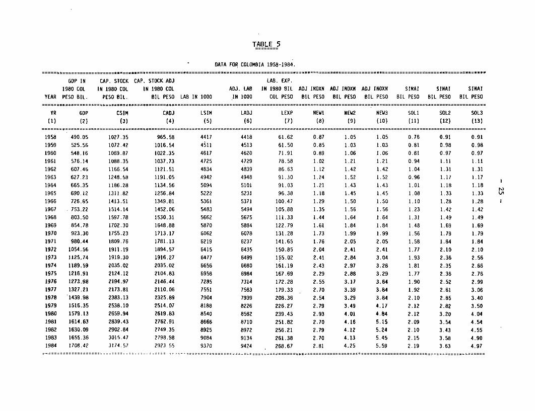
TABLE 5

DATA FOR COLOMBIA 1958-1984.

GDP IN CAP. STOCK CAP. STOCK ADJ LAB. EXP.

1980 COL IN 1980 COL IN 1980 COL ADJ. LAB IN 1980 BIL ADJ INDXN ADJ INDXN ADJ INDXN SINAI SINAI SINAI

YEAR PESO BIL. PESO BIL. BIL PESO LAB IN 1000 IN 1000 COL PESO BIL PESO BIL PESO BIL PESO BIL PESO BIL PESO BIL PESO

YR GDP CSIM CADJ LSIM LADJ LEXP NEW1 NEW2 NEW3 SOL1 SOL2 SOL3

(1) (2) (3) (4) (5) (6) (7) (8) (9) (10) (11) (12) (13)

1958 490.05 1027.35 965.58 4417 4418 61.62 0.87 1.05 1.05 0.76 0.91 0.91

1959 525.56 1072.42 1016.54 4Š11 4513 61.50 0.85 1.03 1.03 0.81 0.98 0.98

1960 548.16 1069.87 1022.35 4617 4620 71.91 0.89 1.06 1.06 0.81 0.97 0.97

1961 576.14 1088.35 1037.73 4725 4729 78.58 1.02 1.21 1.21 0.94 1.11 1.11

1962 607.46 1166.54 1121.51 4834 4839 86.63 1.12 1.42 1.42 1.04 1.31 1,31

1963 627.23 1248.58 1191.05 4942 4948 91.30 1.24 1.52 1.52 0.96 1.17 1.17

1964 665.35 1186.28 1134.56 5094 5101 91.03 1.21 1.43 1.43 1.01 1.18 1.18

1965 690.12 1311.82 1256.84 5222 5231 96.38 1.18 1.45 1.45 1.08 1.33 1.33

1966 726.65 1413.51 1349.81 5361 5371 100.47 1.29 1.50 1.50 1.10 1.28 1.28

1967 753.22 1514.14 1452.06 5483 5494 105.88 1.35 1.56 1.56 1.23 1.42 1.42

1968 803.50 1597.78 1530.31 5662 5675 111.33 1.44 1.64 1.64 1.31 1.49 1.49

1969 854.78 1702.30 1648.88 5870 5884 122.79 1.61 1.84 1.84 1.48 1.69 1.69

1970 923.30 1755.23 1713.17 6062 6078 131.28 1.73 1.99 1.99 1.56 1.79 1.79

1971 980.44 1809.76 1781.13 6219 6237 141.65 1.76 2.05 2.05 1.58 1.84 1.84

1972 1054.56 1911.19 1894.57 6415 6435 150.85 2.04 2.41 2.41 1.77 2.10 2.10

1973 1125.74 1919.30 1916.27 6477 6499 155.02 2.41 2.84 3.04 1.93 2.36 2.56

1974 1189.59 2035.02 2035.02 6656 6680 161.19 2.43 2.97 3.28 1.81 2.35 2.66

1975 1216.91 2124.12 2104.83 6958 6984 167.69 2.29 2.88 3.29 1.77 2.36 2.761976 1273.98 2194.97 2146.44 7285 7314 172.28 2.55 3.17 3.64 1.90 2.52 2.991977 1327.21 2173.81 2110.06 7551 7583 179.33 2.70 3.39 3.84 1.92 2.61 3.061978 1439.98 2383.13 2325.89 7904 7939 208.36 2.54 3.29 3.84 2.10 2.85 3.401979 1516.35 2538.10 2514.07 8188 8226 226.27 2.79 3.49 4.17 2.12 2.82 3.501980 1579.13 2659.94 2619.83 8540 8582 239.43 2.93 4.01 4.84 2.12 3.20 4.041981 1614.63 2839.43 2762.91 8666 8710 251.82 2.70 4.16 5.15 2.09 3.54 4.541982 1630.09 2902.84 2749.35 8925 8972 256.21 2.79 4.12 5.24 2.10 3.43 4.55

1983 1655.36 3015.47 2798.98 9084 9134 261.38 2.70 4.13 5.45 2.15 3.58 4.90

1984 1708.42 3174.57 2923.55 9370 9424 268.67 2.81 4.25 5.59 2.19 3.63 4.97

TABLE 6

NATURAL LOGARITHMIC TRANSFORMATION OF THE VARIABLES

GDP IN CAP. STOCK CAP. STOCK ADJ LAB. EXP.

1980 COL IN 1980 COL IN 1980 COL ADJ. LAB IN 1980 BIL ADJ INDXN ADJ INDXN ADJ INDXN SINAI SINAI SINAI

YEAR PESO BIL. PESO BIL. BIL PESO LAB IN 1000 IN 1000 COL PESO BIL PESO BIL PESO BIL PESO BIL PESO BIL PESO BIL PESO

YR GDP CSIM CADJ LSIM LADJ LEXP NEW1 NEW2 NEW3 SOL1 SOL2 SOL3

(1) (2) (3) (4) (5) (6) (7) (8) (9) (10) (11) (12) (13)

1958 6.19451 6.93474 6.87273 8.39322 8.39342 4.12103 -0.13489 0.04600 0.04600 -0.27597 -0.09508 -0.09508

1959 6.26446 6.97767 6.92416 8.41427 8.41468 4.11902 -0.16639 0.02516 0.02516 -0.21402 -0.02247 -0.02247

1960 6.30657 6.97530 6.92986 8.43750 8.43810 4.27547 -0.11361 0.06200 0.06200 -0.20670 -0.03109 -0.03109

1961 6 35635 6.99242 6.94479 8.46062 8.46143 4.36414 0.01906 0.18901 0.18901 -0.06610 0.10385 0.10385

1962 6.40929 7.06180 7.02243 8.48343 8.48444 4.46163 0.11Z52 0.34890 0.34890 0.03905 0.27043 0.27043

1963 6.44131 7.12976 7.08259 8.50553 8.50674 4.51410 0.21401 0.41830 0.41830 -0.04485 0.15944 0.15944

1964 6.50031 7.07858 7.03400 8.53582 8.53724 4.51121 0.19365 0.35604 0.35604 0.00559 0.16799 0.16799

1965 6.53687 7.17917 7.13636 8.56064 8.56226 4.56830 0.16889 0.37382 0.37382 0.07966 0.28459 0.28459

1966 6.58844 7.25383 7.20772 8.58691 8.58874 4.60988 0.25473 0.40430 0.40430 0.09682 0.24640 0.24640

1967 6.62436 7.32260 7.28074 8.60941 8.61145 4.66231 0.30151 0.44481 0.44481 0.20914 0.35243 0.35243

1968 6.68898 7.37637 7.33323 8.64153 8.64379 4.71249 0.36488 0.49546 0.49546 0.27047 0.40105 0.40105

1969 6.75084 7.43973 7.40785 8.67761 8.68007 4.81049 0.47871 0.60877 0.60877 0.39245 0.52251 0.52251

1970 6.82795 7.47036 7.44610 8.70980 8.71247 4.87730 0.54621 0.68688 0.68688 0.44170 0.58237 0.58237

1971 6.88800 7.50095 7.48501 8.73536 8.73825 4.95339 0.56507 0.71751 0.71751 0.45507 0.60751 0.60751

1972 6.96088 7.55548 7.54674 8.76639 8.76950 5.01626 0.71244 0.88120 0.88120 0.57079 0.73955 0.73955

1973 7.02620 7.55972 7.55814 8.77601 8.77933 5.04353 0.87968 1.04328 1.11251 0.65654 0.85717 0.93999

1974 7.08136 7.61826 7.61826 8.80327 8.80681 5.08261 0.88753 1.08838 1.18681 0.59365 0.85481 0.97760

1975 7.10407 7.66111 7.65199 8.84765 8.85140 5.12213 0.83032 1.05845 1.19043 0.57054 0.85741 1.01656

1976 7.14990 7.69392 7.67157 8.89357 8.89754 5.14912 0.93610 1.15254 1.29217 0.64139 0.92240 1.09519

1977 7.19083 7.68424 7.65447 8.92944 8.93362 5.18922 0.99226 1.22113 1.34502 0.65051 0.95943 1.11758

1978 7.27238 7.77617 7.75186 8.97512 8,97953 5.33928 0.93291 1.18993 1.34531 0.74352 1.04671 1.224011979 .7.32406 7.83917 7.82966 9.01042 9.01505 5.42174 1.02466 1.24961 1.42677 0.74956 1.03634 1.25137

1980 7.36463 7.88606 7.87086 9.05252 9.05737 5.47827 1.07559 1.38939 1.57790 0.75330 1.16462 1.39551

1981 7.38686 7.95136 7.92404 9.06716 9.07224 5.52871 0.99484 1.42473 1.63937 0.73606 1.26417 1.511901982 7.39639 7.97344 7.91912 9.09661 9.10191 5.54598 1.02537 1.41618 1.65680 0.74094 1.23289 1.51563

1983 7.41177 8.01151 7.93701 9.11427 9.11979 5.56597 0.99390 1.41712 1.69591 0.76617 1.27397 1.58951

1984 7.44332 8.06293 7.98056 9.14527 9.15102 5.59347 1.03261 1.44656 1.72150 0.78184 1.28801 1.60342

- 27 -

TABLE ?.

GOP OF COLOMBIA 1958-1984.

GOP IN 1980

COLOMBIAN PESO

YEAR (IN BILLIONS)

1958 490.05

1959 525.561960 548.16

1961 576.14

1962 607.46

1963 627.231964 665.35

1965 690.12

1966 726.651967 753.221968 803.50

1969 854.78

1970 923.30

1971 980.441972 1054.561973 1125.741974 1189.591975 1216.911976 1273.981977 1327.211978 1439.98

1979 1516.35

1980 1579.13

1981 1614.63

1982 1630.091983 1655.361984 1708.42

- 28 -

TABLE 8

CAPITAL STOCK FOR COLOMBIA 1958-1984

CAP. STOCK IN 1980 CUDDINGTON'S INDEX WITH CAPITAL STOCK ADJUSTED

COL. PESO INDEX YEAR 1974=1 FOR CAPACITY UTILIZATION.YEAR (IN BILLIONS) 1980 COL. BIL. PESO

1958 1027.35 98.5676 0.93987 965.581959 1072.42 99.4091 0.94789 1016.541960 1069.87 100.2155 0.95558 1022.351961 1088.35 99.9957 0.95349 1037.731962 1166.54 100.8256 0.96140 1121.511963 1248.58 100.0418 0.95392 1191.051964 1186.28 100.3015 0.95640 1134.561965 1311.82 100.4785 0.95809 1256.841966 1413.51 100.1475 0.95493 1349.811967 1514.14 100.5741 0.95900 1452.061968 1597.78 100.4458 0.95778 1530.311969 1702.30 101.5829 0.96862 1648.881970 1755.23 102.3611 0.97604 1713.171971 1809.76 103.2149 0.98418 1781.131972 1911.19 103.9616 0.99130 1894.571973 1919.30 104.7085 0.99842 1916.271974 2035.02 104.8739 1.00000 2035.021975 2124.12 103.9215 0.99092 2104.831976 2194.97 102.5555 0.97789 2146.441977 2173.81 101.7983 0.97067 2110.061978 2383.13 102.3549 0.97598 2325.891979 2538.10 103.8810 0.99053 2514.07

1980 2659.94 103.2924 0.98492 2619.83

1981 2839.43 102.0476 0.97305 2762.91

1982 2902.84 99.3287 0.94712 2749.35

1983 3015.47 97.3444 0.92820 2798.98

1984 3174.57 96.5815 0.92093 2923.55

- 29 -

TABLE 9.

LABOR FORCE IN COLOMBIA 1958-1984.

NUMBER OF SEX AND EDUC. FRACTION OF LAB IN 1000 LAB. EXP.

PERSONS ADJ. (HANSEN) LABOR FORCE ADJ. FOR IN 1980 BIL

YEAR (LAB IN 1000) 0.5% GROWTH WHICH IS NEW SEX & EDUC. COL PESO

1958 4417 0.00500 0.04000 4418 61.62

1959 4511 0.01003 0.04000 4513 61.50

1960 4617 0.01508 0.04000 4620 71.91

1961 4725 0.02015 0.04000 4729 78.58

1962 4834 0.02525 0.04000 4839 86.63

1963 4942 0.03038 0.04000 4948 91.30

1964 5094 0.03553 0.04000 5101 91.03

1965 5222 0.04071 0.04000 5231 96.381966 5361 0.04591 0.04000 5371 100.47

1967 5483 0.05114 0.04000 5494 105.88

1968 5662 0.05640 0.04000 5675 111.331969 5870 0.06168 0.04000 5884 122.79

1970 6062 0.06699 0.04000 6078 131.28

1971 6219 0.07232 0.04000 6237 141.65

1972 6415 0.07768 n.04000 6435 150.85

1973 6477 0.08307 0.04000 6499 155.02

1974 6656 0.08849 0.04000 6680 161.19

1975 6958 0.09393 0.04000 6984 167.69

1976 7285 0.09940 0.04000 7314 172.28

1977 .7551 0.10490 0.04000 7583 179.33

1978 7904 0.11042 0.04000 7939 208.36

1979 8188 0.11597 0.04000 8226 226.27

1980 8540 0.12155 0.04000 8582 239.43

1981 8666 0.12716 0.04000 8710 251.821982 8925 0.13280 0.04000 8972 256.21

1983 9084 0.13846 0.04000 9134 261.38

1984 9370 0.14415 0:04000 9424 268.67

- 30 -

TABLE 10

MONETARY BALANCES IN COLOMBIA 1958-1984.

MONEY + QUASI CAV M2 + CAVS.

MONEY (MI) MONEY = M2 DEPOSITS = M3YEAR BIL. PESO BIL. PESO BIL. PESO BIL. PESO

1958 3.26 3.91 0.00 3.911959 3.63 4.40 0.00 4.401960 3.99 4.75 0.00 4.751961 4.96 5.88 0.00 5.881962 5.93 7.47 0.00 7.471963 6.69 8.21 0.00 8.211964 8.25 9.70 0.00 9.701965 9.64 11.83 0.00 11.831966 11.24 13.05 0.00 13.051967 13.68 15.79 0.00 15.791968 15.86 18.07 0.00 18.071969 19.40 22.09 0.00 22.091970 22.40 25.78 0.00 25.781971 25.06 29.19 0.00 29.191972 31.85 . 37.71 0.00 37.711973 41.65 50.90 4.40 55.301974 49.07 63.71 8.32 72.031975 58.92 78.49 13.54 92.031976 79.38 105.14 19.83 124.971977 103.30 140.69 24.11 164.801978 132.93 180.01 34.92 214.931979 165.90 221.00 53.02 274.021980 212.40 320.47 83.23 403.701981 256.37 434.73 122.21 556.941982 321.40 525.65 171.76 697.411983 396.74 659.23 244.58 903.811984 492.39 816.84 302.90 1119.74

- 31 -

TABLE 11

REAL MONETARY BALANCES FOR COLOMBIA 1958-1984.

MONEY + QUASI CAV M2 + CAVS. INFLATION REAL MONEY REAL MONEY REAL MONEYMONEY (Ml) MONEY = M2 DEPOSITS = M3 GNP DEFLATOR BASED ON BALANCES BALANCES BALANCES

YEAR BIL. PESO BIL. PESO BIL. PESO BIL. PESO (1980=100) GNP DEFLATOR SOLl SOL2 SOL3

1958 3.26 3.91 0.00 3.91 4.30 13.16% 0.76 0.91 0.911959 3.63 4.40 0.00 4.40 4.50 4.65% 0.81 0.98 0.981960 3.99 4.75 0.00 4.75 4.90 8.89% 0.81 0.97 0.971961 4.96 5.88 0.00 5.88 5.30 8.16% 0.94 1.11 1.111962 5.93 7.47 0.00 7.47 5.70 7.55% 1.04 1.31 1.311963 6.69 8.21 0.00 8.21 7.00 22.81% 0.96 1.17 1.171964 8.25 9.70 0.00 9.70 8.20 17.14% 1.01 1.18 1.181965 9.64 11.83 0.00 11.83 8.90 8.54% 1.08 1.33 1.331966 11.24 13.05 0.00 13.05 10.20 14.61% 1.10 1.28 1.281967 13.68 15.79 0.00 15.79 11.10 8.82% 1.23 1.42 1.421968 15.86 18.07 0.00 18.07 12.10 9.01% 1.31 1.49 1.491969 19.40 22.09 0.00 22.09 13.10 8.26% 1.48 1.69 1.691970 22.40 25.78 0.00 25.78 14.40 9.92% 1.56 1.79 1.791971 25.06 29.19 0.00 29.19 15.90 10.42% 1.58 1.84 1.841972 31.85 37.71 0.00 37.71 18.00 13.21% 1.77 2.10 2.101973 41.65 50.90 4.40 55.30 21.60 20.00% 1.93 2.36 2.561974 49.07 63.71 8.32 72.03 27.10 25.46% 1.81 2.35 2.661975 58.92 78.49 13.54 92.03 33.30 22.88% 1.77 2.36 2.761976 79.38 105.14 19.83 124.97 41.80 25.53% 1.90 2.52 2.991977 103.30 140.69 24.11 164.80 53.90 28.95% 1.92 2.61 3.061978 132.93 180.01 34.92 214.93 63.20 17.25% 2.10 2.85 3.40

1979 165.90 221.00 53.02 274.02 78.40 24.05% 2.12 2.82 3.50

1980 212.40 320.47 83.23 403.70 100.00 27.55% 2.12 3.20 4.04

1981 256.37 434.73 122.21 556.94 122.80 22.80% 2.09 3.54 4.54

1982 321.40 525.65 171.76 697.41 153.20 24.76% 2.10 3.43 4.55

1983 396.74 659.23 244.58 903.81 184.40 20.37% 2.15 3.58 4.90

1984 492.39 816.84 302.90 1119.74 225.30 22.18% 2.19 3.63 4.97

- 32 -

TABLE 12

INDEXED REAL MONEY BALANCES FOR COLOMBIA 1958-1984.

MONEY+QUASI CAV M2 + CAVS. GNP INFLATION PRICE OF PRICE ADJ. PRICE ADJ. PRICE ADJ.

MONEY (Ml) MONEY = M2 DEPOSITS = M3 DEFLATOR BASED ON INFLATION REAL MONEY REAL MONEY REAL MONEY

YR BIL. PESO BIL. PESO BIL. PESO BIL. PESO (1980=100) GNP DEFLATOR 1/1-INFL BAL (NEWI) BAL (NEW2) BAL (NEW3)

1958 3.26 3.91 0.00 3.91 4.30 13.16% 1.15 0.87 1.05 1.05

1959 3.63 4.40 0.00 4.40 4.50 4.65% 1.05 0.85 1.03 1.03

1960 3.99 4.75 0.00 4.75 4.90 8.89% 1.10 0.89 1.06 1.06

1961 4.96 5.88 0.00 5.88 5.30 8.16% 1.09 1.02 1.21 1.21

1962 5.93 7.47 0.00 7.47 5.70 7.55% 1.08 1.12 1.42 1.42

1963 6.69 8.21 0.00 8.21 7.00 22.81% 1.30 1.24 1.52 1.52

1964 8.25 9.70 0.00 9.70 8.20 17.14% 1.21 1.21 1.43 1.43

1965 9.64 11.83 0.00 11.83 8.90 8.54% 1.09 1.18 1.45 1.45

1966 11.24 13.05 0.00 13.05 10.20 14.61% 1.17 1.29 1.50 1.50

1967 13.68 15.79 0.00 15.79 11.10 8.82% 1.10 1.35 1.56 1.56

1968 15.86 18.07 0.00 18.07 12.10 9.01% 1.10 1.44 1.64 1.64

1969 19.40 22.09 0.00 22.09 13.10 8.26% 1.09 1.61 1.84 1.84

1970 22.40 25.78 0.00 25.78 14.40 9.92% 1.11 1.73 1.99 1.99

1971 25.06 29.19 0.00 29.19 15.90 10.42% 1.12 1.76 2.05 2.05

1972 31.85 37.71 0.00 37.71 18.00 13.21% 1.15 2.04 2.41 2.41

1973 41.65 50.90 4.40 55.30 21.60 20.00% 1.25 2.41 2.84 3.04

1974 49.07 63.71 8.32 72.03 27.10 . 25.46% 1.34 2.43 2.97 3.28

1975 58.92 78.49 13.54 92.03 33.30 22.88% 1.30 2.29 2.88 3.29

1976 79.38 105.14 19.83 124.97 41.80 25.53% 1.34 . 2.55 3.17 3.64

1977 103.30 140.69 24.11 164.80 53.90 28.95% 1.41 2.70 3.39 3.84

1978 132.93 180.01 34.92 214.93 63.20 17.25% 1.21 2.54 3.29 3.84

1979 165.90 221.00 53.02 274.02 78.40 24.05% 1.32 2.79 3.49 4.17

1980 212.40 320.47 83.23 403.70 100.00 27.55% 1.38 2.93 4.01 4.84

1981 256.37 434.73 122.21 556.94 122.80 22.80% 1.30 2.70 4.16 5.151982 321.40 525.65 171.76 697.41 153.20 24.76% 1.33 2.79 4.12 5.24

1983 396.74 659.23 244.58 903.81 184.40 20.37% 1.26 2.70 4.13 5.45

1984 492.39 816.84 302.90 1119.74 225.30 22.18% 1.29 2.81 4.25 5.59

- 33 -

YEAR G0P CSIM LSIM TABLE 13 (REGRESSION WITH NO MONEY VARIABLE)1958 490.050.000.000 1.027,355.000,000 4,417,000

1959 525.560,000,000 1,072.422.000.000 4,511.000

1960 548.160,000.000 1,069,874,000.000 4.617.000

1961 576,140.000.000 1,088,350,000,000 4.725.000

1962 607,460.000.000 1,166,541,000,000 4,834.000

1963 627.230,000.000 1,248,580,000,000 4.942.0001964 665.350.000.000 1.186,283,000.000 5,094,000

1965 690.120,000.000 1,311,820,000,000 5,222,000

1966 726.650,000.000 1,413,510,000,000 5,361.000

1967 753,220.000.000 1,514,137.000,000 5,483.000

1968 803,500.000,000 1,597,778.000,000 5.662.000

1969 854,780.000.000 1,702,295.000.000 5.870.000

1970 923.300.000.000 1,755,230.000.000 6,062,000

1971 980.440.000.000 1.809,763.000.000 6.219.000

1972 1.054,560,000.000 1.911,191,000.000 6.415.000

1973 1.125,740,000.000 1.919.299.000.000 6,477.000

1974 1.189,590.000,000 2.035,018.000.000 6.656.000

1975 1.216,910,000,000 2.124.118.000.000 6.958.000

1976 1,273,980,000,000 2.194,967.000000 7.285.000

1977 1,327.210,000,000 2.173,814.000.000 7,551,000

1978 1,439.980,000,000 2.383.128,000.000 7.904,000

1979 1.516,350,000,000 2,538,102,000,000 8.188,000

1980 1,579.130.00,000 2.659,937,000,000 8,540,000

1981 1,614,630.000.000 2,839.431.000,000 8.666,000

1982 1,630,090,000.000 2,902,840,000.000 8.925.000

1983 1.655.360,000000 3.015,472,000.000 9.084,000

1984 1,708,420,000,000 3,174,569,000,000 9.370.000

CALCULATIONS FOR FINDING COMPONENTS OF GROWTH

YEAR q = Q/L k KA q. k. q./q k/k wkk./k A./A A(t)1958 110946.34 232591.13

1959 116506.32 237734.87 5559.974 5143.745 0.05011 0.02211 0.00806 0.04206 1.00000

1960 118726.45 231724.93 2220.128 -6009.941 0.01906 -0.02528 -0.00921 0.02827 1.04206

1961 121934.39 230338.62 3207.946 -1386.305 0.02702 -000598 -0.00218 0.02920 1.07151

1962 125664.05 241320.02 3729.655 10981.400 0.03059 0.04768 0.01737 0.01322 1.10280

1963 126918.25 252646.70 1254.205 11326.677 0.00998 0.04694 0.01710 -0.00712 1.11738

1964 130614.45 232878.48 3696.197 -19768.217 0.02912 -0.07824 -0.02850 0.05763 1.10942

1965 132156,26 251210.26 1541.814 18331.780 0.01180 0.07872 0.02868 -0.01687 1.173361966 135543.74 263665.36 3387.480 12455.097 0.02563 0.04958 0.01806 0.00757 1.153561967 137373.70 276151.19 1829.959 12485.834 0.01350 0.04735 0.01725 -0.00375 1.162291968 141910.99 282193.22 4537.285 6042.023 0,03303 0.02188 0.00797 0.02506 1.5794

1969 145618.40 289999.15 3707.413 7805.930 0.02612 0.02766 0.01008 0.01605 1.86951970 152309.47 289546.35 6691.070 -452.794 0.04595 -0.00156 -0.00057 0.04652 1.206C

1971 157652.36 291005.47 5342.887 1459.113 0.03508 0.00504 0.00184 0.03324 1 262:1972 164389.71 297925.33 6737.356 6919.864 0.04274 0.02378 0.00866 0.03407 1.3C4^E

1973 173805.77 296325.30 9416.063 -1600.026 0.05728 -0.00537 -0.00196 0.05924 1.34841974 178724.46 305741.89 4918.685 9416.582 0.02830 0.03178 0.01158 0.01672 1.42837

1975 174893.65 305277.09 -3830.812 -464.796 -0.02143 -0.00152 -0.00055 -0.02088 1.452Z6

1976 174877.14 301299.52 -16.503 -3977.572 -0.00009 -0.01303 -0.00475 0.00465 1.42193

1977 175766.12 287884.25 888.979 -13415.266 0.00508 -0.04452 -0.01622 0.02130 1.42855

1978 182183.70 301509.11 6417.581 13624.856 0.03651 0.04733 0.01724 0.01927 1.45898

1979 185191.74 309978.26 3008.040 8469.152 0.01651 0.02809 0.01023 0.00628 1.48710

1980 184909.84 311468.03 -281.908 1489.772 -0.00152 0.00481 0.00175 -0.00327 1.49643

1981 186317.79 327651.86 1407.958 '6183.825 0.00761 0.05196 0.01893 -0.01131 1.49154

1982 182643.14 325248.18 -3674.656 -2403.679 -0.01972 -0.00734 -0.00267 -0.01705 1.47466

1983 182228.09 331954.21 -415.044 6706.026 -0.00227 0.02062 0.00751 -0.00978 1.449521984 182328.71 338801.39 100.615 6847.182 0.00055 0.02063 0.00751 -0.00696 1.43534

0.50654 0.14320 0.36334

GROWTH DUE TO: CAPITAL TECHNICAL CHG.100.00% 28.27% 71.73%

- 34 -

TABLE 14

(REGRESSION WITH NEW2 AS INDEPENDENT VARIABLE)

DATA USED FOR USING SOLOW'S APPROACH TO FIND COMPONENTS OF GROWTH

UNADJUSTED NUMBER OF M2 WITH

GOP CAPITAL (CSIM) PERSONS PRICES IN COL PESOYEAR COL 80 PESO COL 80 PESO EMPLOYED NEW2(INDEXATION)

1958 490,050,000,000 1,027,355,000,000 4,417,000 1,047,075,4051959 525,560.000,000 1,072.422.000,000 4,511.000 1.025,474,2551960 548.160,000,000 1,069,874.000,000 4.617,000 1.063,962,1701961 576.140,000,000 1.088,350.000,000 4,725,000 1.208,050,3141962 607,460,000,000 1,166.541,000,000 4,834,000 1,417,508,0561963 627.230,000,000 1,248,580,000,000 4,942,000 1,519,383,1171964 665,350,000,000 1,186,283,000,000 5,094,000 1.427.670,3111965 690,120.000,000 1,311,820,000,000 5,222,000 1,453,273,4081966 726,650,000,000 1,413,510,000.000 5,361,000 1,498.258,5141967 753,220,000,000 1,514,137,000,000 5,483,000 1,560,185.9921968 803,500,000,000 1,597,778,000,000 5,662,000 1,641.248.670

1969 854,780,000.000 1.702.295.000,000 5,870,000 1,838,174,8161970 923,300,000.000 1,755,230.000,000 6,062,000 1,987,511,7701971 980,440,000,000 1,809,763,000.000 6,219,000 2,049,319,8771972 1,054,560,000,000 1,911.191,000,000 6,415,000 2,413,804,348

1973 1,125,740,000,000 1,919,299,000,000 6,477.000 2,838,506,9441974 1,189,590,000,000 2.035,018.000,000 6,656.000 2,969,447,1821975 1.216,910.000,000 2,124,118.000,000 6,958.000 2,881,897.2081976 1,273.980.000,000 2,194,967,000,000 7.285.000 3.166.217,2981977 1,327,210,000.000 2,173,814,000,000 7.551,000 3,391,005,2911978 1.439,980.000,000 2,383,128,000,000 7,904,000 3,286,844,7381979 1,516,350,000,000 2,538,102,000,000 8,188,000 3,488,966,8371980 1,579.130,000,000 2.659.937,000,000 8,540,000 4,012.418,3101981 1,614.630,000.000 2,839,431,000,000 8,666,000 4.156.722.2491982 1,630,090,000,000 2,902,840,000,000 8.925,000 4,121,357.6461983 1,655,360,000,000 3.015,472.000,000 9,084.000 4.125,224,3871984 1,708,420,000,000 3.174,569,000,000 9,370,000 4,248,467,502

TABLE 14 (CONTD)

CALCULATIONS FOR FINDING COMPONENTS OF GROWTH

YEAR q = Q/L k = KI m = M/L q. k. m. q./q k./k m./m wk*k./k um*m./m A./A A(t)

1958 110946.34 232591.13 237.061959 116506.32 237734.87 227.33 5559.974 5143.745 -9.728 0.05011 0.02211 -0.04104 0.00610 -0.01274 0.05675 1.000001960 118726.45 231724.93 230.44 2220.128 -6009.941 3.117 0.01906 -0.02528 0.01371 -0.00697 0.00426 0.02177 1.05675

1961 121934.39 230338.62 255.67 3207.946 -1386.305 25.228 0.02702 -0.00598 0.10947 -0.00165 0.03397 -0.00530 1.07976

1962 125664.05 241320.02 293.24 3729.655 10981.400 31.565 0.03059 0.04768 0.14693 0.01315 0.04560 -0.02816 1.07403

1963 126918.25 252646.70 307.44 1254.205 11326.677 14.206 0.00998 0.04694 0.04845 0.01295 0.01503 -0.01800 1.04378

1964 130614.45 232878.48 280.27 3696.197 -19768.217 -27.178 0.02912 -0.07824 -0.08840 -0.02158 -0.02743 0.07814 1.02499

1965 132156.26 251210.26 278.30 1541.814 18331.780 -1.967 0.01180 0.07872 -0.00702 0.02172 -0.00218 -0.00773 1.10509

1966 135543.74 263665.36 279.47 3387.480 12455.097 1.175 0.02563 0.04958 0.00422 0.01368 0.00131 0.01064 1.09654

1967 137373.70 276151.19 284.55 1829.959 12485.834 5.076 0.01350 0.04735 0.01816 0.01306 0.00564 -0.00520 1.10822

1968 141910.99 282193.22 289.87 4537.285 6042.023 5.321 0.03303 0.02188 0.01870 0.00604 0.00580 0.02119 1.10245 t-

1969 145618.40 289999.15 313.15 3707.413 7805.930 23.276 0.02612 0.02766 0.08030 0.00763 0.02492 -0.00643 1.12581

1970 152309.47 289546.35 327.86 6691.070 -452.794 14.717 0.04595 -0.00156 0.04700 -0.00043 0.01458 0.03180 1.11858

1971 157652.36 291005.47 329.53 5342.887 1459.113 1.662 0.03508 0.00504 0.00507 0.00139 0.00157 0.03212 1.15414

1972 164389.71 297925.33 376.28 6737.356 6919.864 46.749 0.04274 0.02378 0.14187 0.00656 0.04403 -0.00785 1.19121

1973 173805.77 296325.30 438.24 9416.063 -1600.026 61.969 0.05728 -0.00537 0.16469 -0.00148 0.05111 0.00765 1.18186

1974 178724.46 305741.89 446.13 4918.685 9416.582 7.887 0.02830 0.03178 0.01800 0.00877 0.00559 0.01395 1.19090

1975 174893.65 305277.09 414.18 -3830.812 -464.796 -31.946 -0.02143 -0.00152 -0.07161 -0.00042 -0.02222 0.00121 1.20751

1976 174877.14 301299.52 434.62 -16.503 -3977.572 20.437 -0.00009 -0.01303 0.04934 -0.00359 0.01531 -0.01181 1.20897

1977 175766.12 287884.25 449.08 888.979 -13415.266 14.459 0.00508 -0.04452 0.03327 -0.01228 0.01032 0.00704 1.19469

1978 182183.70 301509.11 415.85 6417.581 13624.856 -33.235 0.03651 0.04733 -0.07401 0.01306 -0.02297 0.04642 1.20310

1979 185191.74 309978.26 426.11 3008.040 8469.152 10.262 0.01651 0.02809 0.02468 0.00775 0.00766 0.00110 1.25895

1980 184909.84 311468.03 469.84 -281.908 1489.772 43.731 -0.00152 0.00481 0.10263 0.00133 0.03185 -0.03470 1.26034

1981 186317.79 327651.86 479.66 1407.958 16183.825 9.820 0.00761 0.05196 0.02090 0.01433 0.00649 -0.01321 1.21661

1982 182643.14 325248.18 461.78 -3674.656 -2403.679 -17.882 -0.01972 -0.00734 -0.03728 -0.00202 -0.01157 -0.00613 1.20054

1983 182228.09 331954.21 454.12 -415.044 6706.026 -7.657 -0.00227 0.02062 -0.01658 0.00569 -0.00515 -0.00281 1.19318

1984 182328.71 338801.39 453.41 100.615 6847.182 -0.708 0.00055 0.02063 -0.00156 0.00569 -0.00048 -0.00465 1.18983

0.50654 0.10844 0.22031 0.17779

GROWTH DUE TO CAPITAL MONEY TECHNICAL CHANGE

100.00% 21.41% 43.49% 35.10%

TABLE 13

DATA USED FOR PREDICTING THE VALUES

YEAR 1958 1972 1984

LNY 5.5855724445 5.9410728 6.1828628

(LNY)SQ 31.19862 35.29635 38.22779

LNN 2.68354 3.09442 3.33508

(LNN)SQ 7.20140 9.57544 11.12274

PREDICTED VALUES FOR COLOMBIA FROM CHENERY & SYRQUIN MODEL

========================================= ===========PREDICTED VALUES======COEFFICIENTS: CONSTANT LNY (LNY)SQ LNN (LNN)SQ 1958 1972 1984

SAVINGS -0.34 0.115 -0.006 0.051 -0.007 0.2016 0.2222 0.2339INVESTMENT -0.161 0.085 -0.004 0.013 -0.002 0.2095 0.2239 0.2327URBANIZAT -1.154 0.365 -0.016 0.019 -0.002 0.4221 0.4894 0.5322 o'

PRIMARY 1.966 -0.449 0.027 -0.012 0.001 0.2754 0.2239 0.1931INDUSTRY -0.522 0.154 -0.006 0.053 -0.007 0.2428 0.2781 0.2997

UTILITIES -0.002 0.006 0.001 0.01 -0.002 0.0751 0.0807 0.0844

SERVICES -0.442 0.288 -0.022 -0.051 0.008 0.4010 0.4113 0.4165HIGH20 -0.228 0.292 -0.027 0 0 0.5606 0.5538 0.5452LOW40 0.466 -0.119 0.01 0 0 0.1133 0.1120 0.1125

Y= PER CAPITA INCOME IN 1964 U.S. DOLLARS

LNY= LN OF Y

(LNY)SQ= SQUARE OF LNY

N= POPULATION IN MILLIONS

LNN= LN OF N

(LNN)SQ= SQUARE OF LNN

- 37 -

TABLE 16

RATIO OF M2(BROAOLY DEFINED MONEY) OVER GOP

YEAR ARG BRA CHL COL MEX PER TIME

1974 32.24% 17.66% 22.01% 22.34% NA 27.64% 11975 25.17% 17.92% 21.14% 22.72% NA 26.08% 2

1976 20.91% 15.38% 15.51% 23.'Q% NA 23.27% 3

1977 24.73% 14.60% 15.96% 23.../. 28.38% 21.00% 4

1978 27.99% 14.05% 17.98% 23.63% 29.91% 21.28% 5

1979 30.53% 14.46% 19.02% 23.05% 30.94% 22.00% 6

1980 29.03% 11.19% 21.48% 25.57% 30.32% 25.32% 7

1981 31.96% 11.16% 24.45% 28.09% 32.91% 24.91% 81982 31.12% 10.86% 31.67% 27.93% 32.44% 25.38% 9

1983 33.72% 10.75% 26.43% 29.59% 28.85% 27.83% 101984 31.02% 11.87% 29.43% 29.03% 28.98% 28.41% 11

LN OF THE ABOVE RATIOS AND TIME

YEAR ARG BRA CHL COL MEX PER LNTIME

1974 -1.1318 -1.7341 -1.5136 -1.4986 NA -1.2858 0.0000

1975 -1.3793 -1.7192 -1.5539 -1.4820 NA -1.3439 0.69311976 -1.5650 -1.8718 -1.8634 -1.4490 NA -1.4580 1.0986

1977 -1.3972 -1.9244 -1.8349 -1.4690 -1.2595 -1.5605 1.3863

1978 -1.2734 -1.9622 -1.7157 -1.4425 -1.2071 -1.5473 1.6094

1979 -1.1864 -1.9335 -1.6595 -1.4675 -1.1732 -1.5142 1.79181980 -1.2370 -2.1902 -1.5378 -1.3639 -1.1933 -1.3735 1.9459

1981 -1.1407 -2.1927 -1.4087 -1.2698 -1.1115 -1.3900 2.0794

1982 -1.1674 -2.2197 -1.1497 -1.2756 -1.1257 -1.3712 2.1972

1983 -1.0870 -2.2301 -1.3306 -1.2176 -1.2432 -1.2790 2.3026

1984 -1.1706 -2.1315 -1.2232 -1.2367 -1.2385 -1.2586 2.3979

ARG=ARGENTINA COL=COLOMBIABRA=BRAZIL MEX=MEXICOCHL=CHILE PER=PERU

- 38 -

TABLE 17

REGRESSION RESULTS OF FINANCIAL DEEPENING OVER TIME

COLOMBIA ARGENTINA

Regression Output: Regression Output:

Constant -1.57070939 Constant -1.36728

Std Err of Y Est 0.065490196 Std Err of Y Est 0.140282

R Squared 0.675463875 R Squared 0.148275

No. of Observations 11 No. of Observations 11Degrees of Freedom 9 Degrees of Freedom 9

X Coefficient(s) 0.120294716 X Coefficient(s) 0.074522

Std Err of Coef. 0.027794301 Std Err of Coef. 0.059536

BRAZIL MEXICO

Regression Output: Regression Output:

Constant -1.63614856 Constant -1.22529

Std Err of Y Est 0.082891446 Std Err of Y Est 0.056020

R Squared 0.832083677 R Squared 0.092869

No. of Observations 11 No. of Observations 8

Degrees of Freedom 9 Degrees of Freedom 6

X Coefficient(s) -0.23493487 X Coefficient(s) 0.023592

Std Err of Coef. 0.035179461 Std Err of Coef. 0.030102

CHILE PERU

Regression Output: Regression Output:

Constant -1.77551464 Constant -1.40860

Std Err of Y Est 0.214306234 Std Err of Y Est 0.113555

R Squared 0.247585125 R Squared 0.001979

No. of Observations 11 No. of Observations 11

Degrees of Freedom 9 Degrees of Freedom 9

X Coefficient(s) 0.156519737 X Coefficient(s) 0.006438

Std Err of Coef. 0.090952421 Std Err of Coef. 0.048193

(1)THE DEPENDENT VARIABLE IS BROADLY DEFINED MONETARY BALANCES AS A SHARE OF GROSS DOMESTIC PRODUC-

(2)THE INDEPENDENT VARIABLE IS TIME. WITH 1974=1, 1975=2,....1984=11.

- 39 -

TABLE 18

INFLATION TAX ON MONEY BALANCES AS A SHARE OF INCOME

MONEY (Ml) M1+QUASI=M2 M2+CAVS=M3. GNP IN INFLATION INFL. RATE- TAX DUE TO

BIL. PESO BIL. PESO BIL. PESO BIL. PESO BASED ON NOMINAL INFLATION

YR (NOMINAL) (NOMINAL) (NOMINAL) (NOMINAL) GNP DEFLATOR INTEREST RATE (T1,T2)

1958 3.26 3.91 3.91 20.30 13.16% 8.058% 2.206%

59 3.63 4.40 4.40 23.30 4.65% -0.449% 0.761%

60 3.99 4.75 4.75 26.40 8.89% 3.789% 1.414%

61 4.96 5.88 5.88 30.00 8.16% 3.063% 1.418%62 5.93 7.47 7.47 33.70 7.55% 2.447% 1.461%

63 6.69 8.21 8.21 42.70 22.81% 17.707% 3.629%

64 8.25 9.70 9.70 53.00 17.14% 12.043% 2.676%65 9.64 11.83 11.83 59.90 8.54% 3.437% 1.483%

66 11.24 13.05 13.05 72.40 14.61% 9.507% 2.279%

67 13.68 15.79 15.79 81.60 8.82% 3.724% 1.520%

68 15.86 18.07 18.07 94.40 9.01% 3.909% 1.539%

69 19.40 22.09 22.09 108.30 8.26% 1.164% 1.458%

70 22.40 25.78 25.78 129.90 9.92% 2.824% 1.695%

71 25.06 29.19 29.19 153.10 10.42% 3.317% 1.701%

72 31.85 37.71 37.71 186.00 13.21% 5.608% 2.253%

73 41.65 50.90 55.30 238.70 20.00% 2.908%

74 49.07 63.71 72.03 318.80 25.46% 3.124%

75 58.92 78.49 92.03 398.60 22.88% 2.752%

76 79.38 105.14 124.97 523.20 25.53% 3.085%

77 103.30 140.69 164.80 708.30 28.95% 3.274%

78 132.93 180.01 214.93 901.60 17.25% 2.170%

79 165.90 221.00 274.02 1181.60 24.05% 2.722%

80 212.40 320.47 403.70 1573.40 27.55% 2.916%

81 256.37 434.73 556.94 1972.30 22.80% 2.413%

82 321.40 525.65 697.41 2459.80 24.76% 2.593%

83 396.74 659.23 903.81 2982.70 20.37% 2.251%

84 492.39 816.84 1119.74 3757.50 22.18% 2.379%

FIGURE 1

INFLATION TAX ON MONETARY BALANCESAS A SHARE OF INCOME

(COLOMBIA:1958-1984)

30%

25%- +5% + +

20%-

15% - + INFLATION

10%_

5% - +INFLATION TAX10%0

1958 60 62 64 66 68 70 72 74 76 78 80 82 84

YEAR

- INFLATION TAX - INFLATION

- 41 -

BIBLIOGRAPHY

Bailey, M.J. "The Welfare Cost of Inflationary Finance." Journal of PoliticalEconomy. Vol. LXIV, No. 2, April 1956.

Barro, R.J. "Monetary Correction, Capital Markets and Open-Market Operationsin Colombia." Journal of Economic Studies. Vol. 2, No. 1, May 1975,pp. 1-9.

Berry, R.A. and M. Urrutia. Income Distribution in Colombia. New Haven: YaleUniversity Press, 1976.

Berry, R.A. and R. Soligo. Economic Policy and Income Distribution in Colombia.Westview Press, 1980.

Carrizosa, M., C. Fajardo and R. Suescun. Analisis economico del sistema devalor constante en colombia. Centro de Estudios sobre DesarrolloEconomico, Universidad de los Andes, December 1982.

Chenery, H.B. and M. Syrquin. Patterns of Development, 1950-1970. Oxford:Oxford University Press, 1975.

Correa, M.C. "Consideraciones sobre el regimen de inversiones por zonas del

sistema bancario y el impuesto inflacionario." Ensavos sobre politicaeconomica. No. 9, June 1986, pp. 11-42.

Cuddington, J. "Bonanzas de productos sasicos, establizacion macroeconomica yreforma comercial en colombia." Ensavos sobre politica economica. No. 10,December 1986, pp. 4 5 -1 0 0 .

Currie, L. and F. Rosas. UPAC - A Theory Converted into a Successful Reality

(Colombian System of Savings and Housing). Bogota: Instituto Colombianode Ahorro y Vivienda, 1986.

Currie, L. "The 'Leading Sector' Model of Growth in Developing Countries."Journal of Economic Studies. May 1974.

Dailami, M. "Policy Changes that Encourage Private Business Investment in

Colombia." World Bank Staff Working Paper. Washington, D.C.: The WorldBank, August 1989.

Elias, V.J. "Sources of Economic Growth in Latin American Countries." Review

of Economics and Statistics. Vol. LX, No. 3, August 1978, pp. 362-370.

Fischer, S. "The Demand for,Index Bonds." Journal of Political Economy.Vol. 83, No. 3, June 1975.

Fry, M. Money, Interest and Banking in Economic Development. Baltimore: Johns

Hopkins University Press, 1988.

- 42 -

Hanson, J.A., F.D. McCarthy and J.A. Kwon. "Sources of Growth in Colombia, 196380." Journal of Economic Studies. Vol. 12, No. 4, 1985, pp. 3-14.

Harberger, A. "La Tasa de rendimiento de capital en colombia." Revista dePlaneacion y desarrollo. Vol. 2, No 1, 1969.

Isaza, F.G. El Upac la politica economica y la construccion 1970-87. Bogota:CAMACOL, 1987.

Jorgenson, D.W. and Z. Griliches. "The Explanation of Productivity Change."Review of Economic Studies. Vol. XXXIV(3), No. 99, 1967, pp. 249-283.

Khan, A.H. and M. Ahmad. "Real Money Balances in the Production Function of aDeveloping Country." Review of Economics and Statistics. Vol. XVII, No. 2,May 1985, pp. 336-340.

Levhari, D. and D. Patinkin. "The Role of Money in a Simple Growth Model."American Economic Review. No. 58, September 1968, pp. 713-754.

Montenegro, A. and M.A. Garcia. "Evolucion del Coeficiente Efectivo-m."Economia Nacional. January 1986, pp. 32-39.

Reyes. "Tendencias del empleo y la distribucion del ingreso." El Problemalaboral colombiano. 1987.

Romer, P.M. "Crazy Explanations for the Productivity Slowdown." NBERMacroeconomics Annual, 1987.

Sandilands, R.J. Monetary Correction and Housing Finance in Colombia, Braziland Chile. England: Gower Publishing Co., 1980.

Short, E.D. "A New Look at Real Money Balances as a Variable in the ProductionFunction." Journal of Money, Credit and Banking. Vol. 11, No. 3,August 1979, pp. 326-339.

Sinai, A. and H.H. Stokes. "Money and the Production Function - A Reply to Boyesand Kavanaugh." Review of Economics and Statistics. Vol. LXIII, No. 2,May 1981, pp. 313-318.

Sinai, A. and H.H. Stokes. "Real Money Balances: An Omitted Variable from theProduction Function?" Review of Economics and Statistics. No. 54,August 1972, pp. 290-296.

Sinai, A. and H.H. Stokes. "Real Money Balances as a Variable in the ProductionFunction - A Further Reply by Allen Sinai and Houston Stokes." Journalof Money, Credit and Banking. Vol. 9, May 1977, pp. 372-373.

Solow, R.M. "Technical Change and the Aggregate Production runction." Reviewof Economics and Statistics. Vol. 39, No. 3, August 1957, pp. 312-320.

Solow, R.M. "Nobel Address." American Economic Review. June 1988, pp. 307-317.

- 43 -

Urrutia, M. Winners and Losers in Colombia's Economic Growth of the 1970s.Oxford: Oxford University Press, 1985.

World Bank. Colombia: Economic Development and Policy Under Changing Conditions.Washington, D.C.: The World Bank, 1983.

World Bank. Colombia: Country Economic Memorandum. Report No. 6626-CO.Washington, D.C.: The World Bank, October 1987.

World Bank. Shelter. Washington, D.C.: The World Bank, 1980.