11

The Aggregate Supply/Aggregate Demand The Aggregate Supply/Aggregate Demand ModelModel

© 2018 Gary R. Evans. This slide set by Gary R. Evans is licensed under a Creative Commons Attribution-NonCommercial-ShareAlike 4.0 International License.

22

33

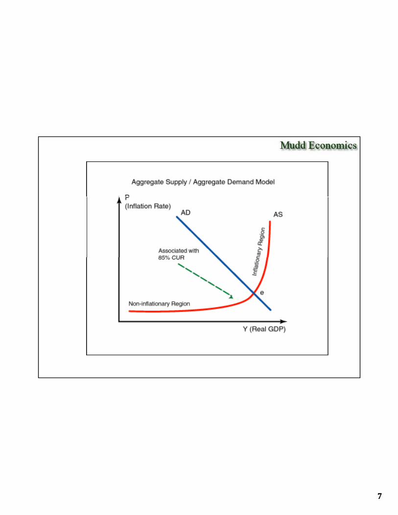
Justifying the Demand Curve: AssumptionsJustifying the Demand Curve: Assumptions

1. Start with a “steady-state” equilibrium economy (then shock it later)

2 Primal source of nominal aggregate demand is nominal national income2. Primal source of nominal aggregate demand is nominal national income earned in the previous period. This prior income becomes our budget constraint (B) in the current period.

3. Nominal national income earned in the previous period equaled nominal GDP in the previous period, which in turn equaled Real GDP (Y) times the Price Level in that period. p

4. In this period we have normalized that price level to a Price Index (Pi ) with a base of 100.

5. In this period we also normalize the Real GDP level to 1 (maybe that represents $100 billion).

6. The two assumptions above, given that we are at steady state, implies that p g y pour nominal budget constraint is 100, which is equal to the current price index times Real GDP.

44

Deriving the Aggregate Demand Curve as a Deriving the Aggregate Demand Curve as a Function of a Price DeflatorFunction of a Price Deflator

Price The assumptions on the

PPBY 100

Index The assumptions on the previous page implies that we are constrained by the following budget constraint:

ii PPY

Real GDP (Y)

55

Transforming the Price Deflator to an Inflation Transforming the Price Deflator to an Inflation Rate (continuous rather than discrete)Rate (continuous rather than discrete)

Price Inflation

iP

PIR ln

Price Inflation Rate (P)

Real GDP (Y)

66

So how do we shock out of the steady state?So how do we shock out of the steady state?

Price Inflation

Easy to answer: Our primary budget constraint is based upon nominal national income from the Price Inflation

Rate (P)previous period. But new credit allows us to expand it out. So do exports. Net savings on the other hand contracts it. Clearly anything that influences aggregate net purchasing power will shock this out, which is why the expansion of reasonable and moderate credit is essential to economic growth.

Real GDP (Y)

77

88

95

100

The Capacity Utilization Rate and the KinkThe Capacity Utilization Rate and the Kink

80

85

90

95

65

70

75

Notable: no inflationary pressure

here!

60

1970

Q1

1973

Q1

1976

Q1

1979

Q1

1982

Q1

1985

Q1

1988

Q1

1991

Q1

1994

Q1

1997

Q1

2000

Q1

2003

Q1

2006

Q1

2009

Q1

2012

Q1

2015

Q1

Source: Federal Reserve Board of Governors, Series G-17 data. Capacity Utilization all industries, SA, quarterly. 1970-2017Q4, Red lines are peaks of business cycles.

99

80

Monthly data .. the weakness in Monthly data .. the weakness in manufacturing 2017 continuing ...manufacturing 2017 continuing ...

After 2013 we were climbing

78

79After 2013 we were climbing as we normally do ..

75

76

77

... but in late 2014 it turned down and continues to decay in 2017. This may be due in part to a

74

75

2012-01 2012-07 2013-01 2013-07 2014-01 2014-07 2015-01 2015-07 2016-01 2016-07

Source: Federal Reserve Board of Governors, Series G-17 data. Capacity Utilization all industries, SA, quarterly. 2012-2016 Dec (monthly data)

y p"strong dollar," a topic that we will cover in a few weeks.

1010

12.5

13.0

... motor vehicle assemblies cooled off but recently picked up some. ... motor vehicle assemblies cooled off but recently picked up some.

11.5

12.0

12.5

10.0

10.5

11.0

Total motor vehicle assemblies, annualized rate, with 6-month moving average, 2012 - 2016.

9.0

9.5

2012-01 2012-07 2013-01 2013-07 2014-01 2014-07 2015-01 2015-07 2016-01 2016-07 2017-01 2017-07

1111

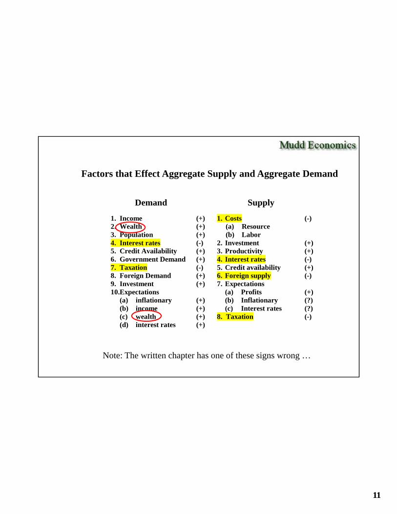
Factors that Effect Aggregate Supply and Aggregate Demand

1. Income2. Wealth3. Population4. Interest rates5. Credit Availability6 G D d

(+)(+)(+)(-)(+)( )

1. Costs(a) Resource(b) Labor

2. Investment3. Productivity4 I

(-)

(+)(+)( )

Demand Supply

6. Government Demand7. Taxation8. Foreign Demand9. Investment10. Expectations

(a) inflationary(b) income(c) wealth

(+)(-)(+)(+)

(+)(+)(+)

4. Interest rates5. Credit availability6. Foreign supply7. Expectations

(a) Profits(b) Inflationary(c) Interest rates

8 Taxation

(-)(+)(-)

(+)(?)(?)(-)(c) wealth

(d) interest rates(+)(+)

8. Taxation (-)

Note: The written chapter has one of these signs wrong …

1212

The core mathematical model

AS f w rc I IR IE etc

AS

( , , , , , )

(-) (-) (+) (-) (?)

whereAS

wand

AD g I W P IR etc and

( , , , , )

0

AS AD

1313

Questions to be answered

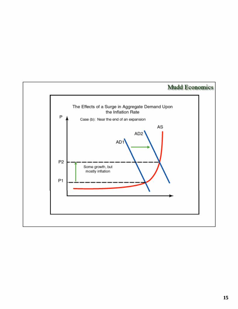
• What causes inflation?

• How can there be inflation with recession?

• What is the role of inflationary yexpectations?

• What is the effect of productivity changes?

• When are wage increases justified?

• What is the pathology of business cycles?

1414

1515

1616

1717

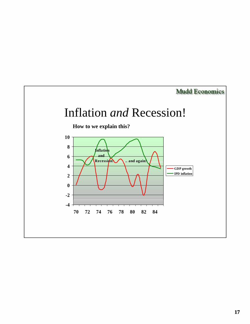
Inflation and Recession!

6

8

10

Inflation andRecession! .. and again!

How to we explain this?

-2

0

2

4 GDP growth

IPD inflation

Recession! .. and again!

-470 72 74 76 78 80 82 84

1818

1919

SupplySupply--side shock: The OPEC oil embargoes of side shock: The OPEC oil embargoes of 1973 & 1979 impact upon gasoline prices in U.S.1973 & 1979 impact upon gasoline prices in U.S.

10.0 Blue represents the monthly percentage change of gasoline

4.0

6.0

8.0prices, U.S. City Average, from the Consumer Price Index.

Source: Bureau of Labor Statistics, Consumer Price Index, all urban consumers, gasoline all types, U.S. city average, SA, series CUSR0000SETB01, monthly growth rate.

-4.0

-2.0

0.0

2.0

Red represents a 12-month moving average Remembering that these are

-8.0

-6.0

1967 1968 1969 1970 1971 1972 1973 1974 1975 1976 1977 1978 1979 1980 1981 1982 1983 1984 1985

average. Remembering that these are monthly rates, note the peaks after 1973 and 1979.

2020

2121

2222

2323

What is "productivity?"What is "productivity?"

Productivity is both difficult to define and measure. It is meant to imply that if you have a given vector of resources, including labor, to produce a vector of outputs, productivity is said to rise if, over time, you get proportionately more output for any measure of inputs. The largest contribution to productivity will be due to the application of technology to production (including the production of services).

A relevant and commonly used measure of national productivity is the measure of Gross Domestic Product per amount of labor time Many economists use theof Gross Domestic Product per amount of labor time. Many economists use the OECD Annual National Accounts database for international comparisons.

For the United States, we use the Bureau of Labor Statistics output-per-hour and unit labor costs.

2424

4.0

5.0

Labor Productivity

1.0

2.0

3.0

-2.0

-1.0

0.0

Is this graph actually telling us anything? Maybe, maybe not. If the annual data are smoothed over 5 years then we see that this figure rose sharply after 1995, then seemed to peak in 2002, erratically moving down since.

-3.01970 1975 1980 1985 1990 1995 2000 2005 2010 2015

Labor Productivity 5 per. Mov. Avg. (Labor Productivity)

U.S. Department of Labor, Bureau of Labor Statistics, Major Sector Labor Productivity as measured by output per hour, precentagechange of previous year, 1970-2016 Series ID PRS84006092. Kept in CU file.

2525

And what about services productivity??And what about services productivity??

Education sector??Seriously??How can anyone possibly claim that productivity is stagnant in education??

Well at least we are better than lawyers and doctors.

2626

This is obviously the ideal situtation that you want ...

2727

4.5

BLS Employment Cost IndexBLS Employment Cost IndexTotal compensation, all civilian, annualized % Total compensation, all civilian, annualized % change, quarterlychange, quarterly, 2001, 2001--2017q3, 2017q3, NSANSA

3.0

3.5

4.0This is inverse to what is called “productivity” and is probably the variable that most mitigates any inflation threat.

... shown with 2-yr MA.

1 0

1.5

2.0

2.5

0.0

0.5

1.0

2001 2002 2003 2004 2005 2006 2007 2008 2009 2010 2011 2012 2013 2014 2015 2016 2017

Source: BLS Employment Cost Index database, CIU1010000000000A (inflation file)

This progress is mostly technological (computing, robotics, the internet) – anything that reduces the labor component of cost.

2828

2929

The The Recession in 2008Recession in 2008--20102010

AD1AD1AD2AD2Due to credit contraction and severe wealth effects, including expectations

3030

The U.S. Economy in 2018: The U.S. Economy in 2018: DeficitDeficit--financed spending?financed spending?

PPPP

ADAD20162016

ADAD20172017 ASAS

2% 2% driftdrift

A t D dAggregate Demand curve shifting out on net due to extremely aggressive fiscal stimulus, possibly “monetized.”

RGDPRGDP