Testing Linear Factor Pricing Models with Large Cross-Sections:

A Distribution-Free Approach

Sermin Gungor Richard Luger†

Bank of Canada Georgia State University

February 9, 2012

Abstract

We develop a finite-sample distribution-free procedure to test the beta-pricing representation of

linear factor pricing models. In sharp contrast to extant finite-sample tests, our framework allows for

unknown forms of non-normalities, heteroskedasticity, and time-varying covariances. The power of

the proposed test procedure increases as the time series lengthens and/or the cross-section becomes

larger. So the criticism sometimes heard that non-parametric tests lack power does not apply here,

since the number of test assets is chosen by the user. This also stands in contrast to the usual tests

that lose power or may not even be computable if the number of test assets is too large.

JEL classification: C12; C14; C33; G11; G12

Keywords: Factor model; Beta pricing; CAPM; Mean-variance efficiency; Robust inference

†Corresponding author. By mail: Department of Risk Management and Insurance, Georgia State University, P.O.

Box 4036, Atlanta, GA 30302-4036, United States. Tel.: 404-413-7489. Fax: 404-413-7499. By e-mail: rluger@gsu.edu

(R. Luger).

1 Introduction

Many asset pricing models predict that expected returns depend linearly on “beta” coefficients

relative to one or more portfolios or factors. The beta is the regression coefficient of the asset

return on the factor. In the capital asset pricing model (CAPM) of Sharpe (1964) and Lintner

(1965), the single beta measures the systematic risk or co-movement with the returns on the

market portfolio. Accordingly, assets with higher betas should offer in equilibrium higher expected

returns. The Arbitrage Pricing Theory (APT) of Ross (1976), developed on the basis of arbitrage

arguments, can be more general than the CAPM in that it relates expected returns with multiple

beta coefficients. Merton (1973) and Breeden (1979) develop models based on investor optimization

and equilibrium arguments that also lead to multiple-beta pricing.

Empirical tests of the validity of beta pricing relationships are often conducted within the

context of multivariate linear factor models. When the factors are traded portfolios and a riskfree

asset is available, exact factor pricing implies that the vector of asset return intercepts will be zero.

These tests are interpreted as tests of the mean-variance efficiency of a benchmark portfolio in the

single-beta model or that some combination of the factor portfolios is mean-variance efficient in

multiple-beta models. In this context, standard asymptotic theory provides a poor approximation

to the finite-sample distribution of the usual Wald and likelihood ratio (LR) test statistics, even

with fairly large samples. Shanken (1996), Campbell, Lo, and MacKinlay (1997), and Dufour and

Khalaf (2002) document severe size distortions for those tests, with overrejections growing quickly

as the number of equations in the multivariate model increases. The simulation evidence in Ferson

and Foerster (1994) and Gungor and Luger (2009) shows that tests based on the Generalized

Method of Moments (GMM) a la MacKinlay and Richardson (1991) suffer from the same problem.

As a result, empirical tests of beta-pricing representations can be severely affected and can lead to

spurious rejections of their validity.

The assumptions underlying standard asymptotic arguments can be questionable when deal-

ing with financial asset returns data. In the context of the consumption CAPM for example,

1

Kocherlakota (1997) shows that the model disturbances are so heavy-tailed that they do not satisfy

the Central Limit Theorem. In such an environment, standard methods of inference can lead to

spurious rejections even asymptotically and Kocherlakota instead relies on jackknifing to devise a

method of testing the consumption CAPM. Similarly, Affleck-Graves and McDonald (1989) and

Chou and Zhou (2006) suggest the use of bootstrap techniques to provide more robust and reliable

asset pricing tests.

There are very few methods that provide truly exact, finite-sample tests.1 The most prominent

one is probably the F-test of Gibbons, Ross, and Shanken (1989) (GRS). The exact distribution

theory for that test rests on the assumption that the vectors of model disturbances are independent

and identically distributed (i.i.d.) each period according to a multivariate normal distribution.

As we already mentioned, there is ample evidence that financial returns exhibit non-normalities;

for more evidence, see Fama (1965), Blattberg and Gonedes (1974), Hsu (1982), Affleck-Graves

and McDonald (1989), and Zhou (1993). Beaulieu, Dufour, and Khalaf (2007) generalize the

GRS approach for testing mean-variance efficiency. Their simulation-based approach does not

necessarily assume normality but it does nevertheless require that the disturbance distribution be

parametrically specified, at least up to a finite number of unknown nuisance parameters. Gungor

and Luger (2009) propose exact tests of the mean-variance efficiency of a single reference portfolio,

whose exactness does not depend on any parametric assumptions.

In this paper we extend the idea of Gungor and Luger (2009) to obtain tests of multiple-beta

pricing representations that relax three assumptions of the GRS test: (i) the assumption of iden-

tically distributed disturbances, (ii) the assumption of normally distributed disturbances, and (iii)

the restriction on the number of test assets. The proposed test procedure is based on finite-sample

pivots that are valid without any assumptions about the specific distribution of the disturbances

in the factor model. We propose an adaptive approach based on a split-sample technique to ob-

tain a single portfolio representation judiciously formed to avoid power losses that can occur in

1A number of Bayesian approaches have also been proposed. These include Shanken (1987), Harvey and Zhou

(1990), and Kandel, McCulloch, and Stambaugh (1995).

2

naive portfolio groupings. For other examples of split-sample techniques, see Dufour and Taamouti

(2005), Jouneau-Sion and Torres (2006), and Dufour and Taamouti (2010).

A very attractive feature of our approach is that it is applicable even if the number of test

assets is greater than the length of the time series. This stands in sharp contrast to the GRS test

or any other approach based on usual estimates of the disturbance covariance matrix. In order to

avoid singularities and be computable, those approaches require the size of the cross-section be less

than that of the time series. In fact, great care must be taken when applying the GRS test since

its power does not increase monotonically with the number of test assets and all the power may be

lost if too many are included. This problem is related to the fact that the number of covariances

that need to be estimated grows rapidly with the number of included test assets. As a result, the

precision with which this increasing number of parameters can be estimated deteriorates given a

fixed time-series.2

Our proposed test procedure then exploits results from Coudin and Dufour (2009) on median

regressions to construct sign-based statistics, one of which is the sign analogue of the usual F-test.

The motivation for using signs comes from an impossibility result due to Lehmann and Stein (1949)

that shows that the only tests which yield reliable inference under sufficiently general distributional

assumptions, allowing non-normal, possibly heteroskedastic, independent observations are based on

sign statistics. This means that all other methods, including the standard heteroskedasticity and

autocorrelation-corrected (HAC) methods developed by White (1980) and Newey and West (1987)

among others, which are not based on signs, cannot be proved to be valid and reliable for any

sample size.

The paper is organized as follows. Section 2 presents the linear factor model used to describe

the asset returns, the null hypothesis to be tested, and the benchmark GRS test. We provide an

illustration of the effects of increasing the number of test assets on the power of the GRS test. In

Section 3 we develop the new test procedure. We begin that section by presenting the statistical

2The notorious noisiness of unrestricted sample covariances is a well-known problem in the portfolio management

literature; see Michaud (1989), Jagannathan and Ma (2003), and Ledoit and Wolf (2003, 2004), among others.

3

framework and then proceed to describe each step of the procedure. Section 4 contains the results

of simulation experiments designed to compare the performance of the proposed test procedure

with several of the standard tests. In Section 5 we apply the procedure to test the Sharpe-Lintner

version of the CAPM and the well-known Fama-French three factor model. Section 6 concludes.

2 Factor model

Suppose there exists a riskless asset for each period of time and define rt as an N × 1 vector of

time-t returns on N assets in excess of riskless rate of return. Suppose further that those excess

returns are described by the linear K-factor model

rt = a+Bft + εt, (1)

where ft is a K×1 vector of common factor portfolio excess returns, B is the N×K matrix of betas

(or factor loadings), and a and εt are N × 1 vectors of factor model intercepts and disturbances,

respectively. Although not required for the proposed procedure, the vector εt is usually assumed

to have well-defined first and second moments satisfying E[εt|ft] = 0 and E[εtε′t|ft] = Σ, a finite

N ×N matrix.

Exact factor pricing implies that expected returns depend linearly on the betas associated to

the factor portfolio returns:

Et[rt] = Bλ, (2)

where λ is a K×1 vector of expected excess returns associated with ft, which represent market-wide

risk premiums since they apply to all traded securities. The beta-pricing representation in (2) is a

generalization of the CAPM of Sharpe (1964) and Lintner (1965), which asserts that the expected

excess return on an asset is linearly related to its single beta. This beta measures the asset’s

systematic risk or co-movement with the excess return on the market portfolio—the portfolio of all

invested wealth. Equivalently, the CAPM says that the market portfolio is mean-variance efficient

in the investment universe comprising all possible assets.3 The pricing relationship in (2) is more

3A benchmark portfolio with excess returns rp is said to be mean-variance efficient with respect to a given set of

4

general since it says that a combination (portfolio) of the factor portfolios is mean-variance efficient;

see Jobson (1982), Jobson and Korkie (1982, 1985), Grinblatt and Titman (1987), Shanken (1987),

and Huberman, Kandel, and Stambaugh (1987) for more on the relation between factor models

and mean-variance efficiency.

The beta-pricing representation in (2) is a restriction on expected returns which can be assessed

by testing the hypothesis

H0 : a = 0 against H1 : a 6= 0, (3)

under the maintained factor structure specification in (1). If the pricing errors, a, are in fact

different from zero, then (2) does not hold meaning that there is no way to combine the factor

portfolios to obtain one that is mean-variance efficient.

GRS propose a multivariate F-test of (3) that all the pricing errors are jointly equal to zero.

Their test assumes that the vectors of disturbance terms εt, t = 1, ..., T , in (1) are independent and

normally distributed around zero with non-singular cross-sectional covariance matrix each period,

conditional on the T ×K collection of factors F = [f ′1, ...,f

′T ]

′. Under normality, the methods of

maximum likelihood and ordinary least squares (OLS) yield the same unconstrained estimates of

a and B:

a = r− Bf , (4)

B =

[T∑

t=1

(rt − r)(ft − f)′

][T∑

t=1

(ft − f)(ft − f)′

]−1

, (5)

where r = T−1∑T

t=1 rt and f = T−1∑T

t=1 ft, and the estimate of the disturbance covariance matrix

is

Σ =1

T

T∑

t=1

(rt − a− Bft)(rt − a− Bft)′. (6)

The GRS test statistic is

J1 =T −N −K

N

[1 + f ′Ω−1f

]−1a′Σ−1a, (7)

N test assets with excess returns rt if it is not possible to form another portfolio of those N assets and the benchmark

portfolio with the same variance as rp but a higher expected return.

5

where Ω is given by

Ω =1

T

T∑

t=1

(ft − f)(ft − f)′.

Under the null hypothesis H0, the statistic J1 follows a central F distribution with N degrees of

freedom in the numerator and (T −N −K) degrees of freedom in the denominator.

In practical applications of the GRS test, one needs to decide the appropriate number N of

test assets to include. It might seem natural to try to use as many test assets as possible in order

to increase the probability of rejecting H0 when it is false. As the test asset universe expands it

becomes more likely that non-zero pricing errors will be detected, if indeed there are any. However,

the choice of N is restricted by T in order to keep the estimate of the disturbance covariance matrix

in (6) from becoming singular, and the choice of T itself is often restricted owing to concerns about

parameter stability. For instance, it is quite common to see studies where T = 60 monthly returns

and N is between 10 and 30. The effects of increasing the number of test assets on test power is

discussed in GRS, Campbell, Lo, and MacKinlay (1997, p. 206) and Sentana (2009). When N

increases, three effects come into play: (i) the increase in the value of J1’s non-centrality parameter,

which increases power, (ii) the increase in the number of degrees of freedom of the numerator, which

decreases power, and (iii) the decrease in the number of degrees of freedom of the denominator due

to the additional parameters that need to be estimated, which also decreases power.

To illustrate the net effect of increasing N on the power of the GRS test, we simulated model

(1) with K = 1, where the returns on the single factor are random draws from the standard

normal distribution. The elements of the independent disturbance vector were also drawn from the

standard normal distribution thereby ensuring the exactness of the GRS test. We set T = 60 and

considered ai = 0.05, 0.10, and 0.15 for i = 1, ..., N and we let the number of test assets N range

from 1 to 58. The chosen values for ai are well within the range of what we find with monthly

stock returns. Figure 1 shows the power of the GRS test as a function of N , where for any given

N the higher power is associated with higher pricing errors. In line with the discussion in GRS,

this figure clearly shows the power of the test given this specification rising as N increases up to

6

about one half of T and then decreasing beyond that. The results in Table 5.2 of Campbell, Lo,

and MacKinlay (1997) show several other alternatives against which the power of the GRS test

declines as N increases. Furthermore, there are no general results about how to devise an optimal

multivariate test. So great care must somehow be taken when choosing the number of test assets

since power does not increase monotonically with N and if the cross-section is too large, then the

GRS test may lose all its power or may not even be computable. In fact, any procedure that relies

on standard unrestricted estimates of the covariance matrix of regression disturbances will have

this singularity problem when N exceeds T .

3 Test procedure

In this section we develop a procedure to test H0 in (3) that relaxes three assumptions of the GRS

test: (i) the assumption of identically distributed disturbances, (ii) the assumption of normally

distributed disturbances, and (iii) the restriction on the number of test assets.

To motivate our approach, consider the problem of testing the following hypothesis:

H(0)0 : u1, ..., uT are independent random variables each with a distribution symmetric

around zero.

Note that H(0)0 allows for the presence of heteroskedasticity of unknown form. The following

characterization of heteroskedasticity-robust tests, taken from Dufour (2003), is due to Lehmann

and Stein (1949); see also Pratt and Gibbons (1981, p. 218) and Dufour and Hallin (1991).

Theorem (Lehmann and Stein 1949). If a test has level α for H(0)0 , where 0 < α < 1, then it

must satisfy the condition

Pr[Rejecting H

(0)0

∣∣ |u1|, ..., |uT |]≤ α under H

(0)0 .

In words, this theorem from classical non-parametric statistics states that the only tests which

yield valid inference under sufficiently general distributional assumptions, allowing non-normal,

7

possibly heteroskedastic, independent observations are ones that are conditional on the absolute

values of the observations; i.e., they must be based on sign statistics. Conversely, if a test procedure

does not satisfy the condition in the above theorem for all levels 0 < α < 1, then its true size is

1 irrespective of its nominal size (Dufour, 2003). With this characterization in mind, we next

present the statistical framework and then proceed to describe each step of the proposed inference

procedure.

3.1 Statistical framework

As in the GRS framework, we assume that the disturbance vectors εt in (1) are independently

distributed over time, conditional on F. We do not require the disturbance vectors to be identically

distributed, but we do assume that they satisfy a multivariate symmetry condition each period. In

what follows the symbold= stands for the equality in distribution.

Assumption 1. The cross-sectional disturbance vectors εt, t = 1, ..., T , are mutually independent,

continuous, and reflectively symmetric so that εtd= −εt, conditional on F.

The reflective symmetry condition in Assumption 1 can be equivalently expressed in terms of

the density function, if it exists, as ft(εt) = ft(−εt). Recall that a random variable εt is symmetric

around zero if and only if εtd= −εt, so the symmetry assumption made here represents the most

direct non-parametric extension of univariate symmetry; see Serfling (2006) for more concepts of

multivariate symmetry.

The class of distributions encompassed by Assumption 1 includes elliptically symmetric distri-

butions, which play a very important role in mean-variance analysis because they guarantee full

compatibility with expected utility maximization regardless of investor preferences; see Chamber-

lain (1983), Owen and Rabinovitch (1983), and Berk (1997). The random vector εt is said to be

elliptically symmetric if there exists a non-singular N × N matrix At such that the unit vector

Atεt/‖Atεt‖ is distributed uniformly on SN , the unit spherical shell of RN , and Atεt/‖Atεt‖ is

independent of ‖Atεt‖. Here ‖ · ‖ stands for the Euclidean norm. The class of elliptically symmet-

8

ric distributions includes the well-known multivariate normal and Student-t distributions, among

many others. From these characterizations, it is easy to see that the following relation holds among

the classes of distributions:

elliptical symmetry ⊂ reflective symmetry;

see also Neuhaus and Zhu (1999). So obviously the reflective symmetry condition in Assumption

1 is less stringent than elliptical symmetry. For instance, a mixture (finite or not) of distributions

each one elliptically symmetric around the origin is not necessarily elliptically symmetric but it is

reflectively symmetric. Note also that the distribution of ft in (1) may be skewed thereby inducing

asymmetry in the unconditional distribution of rt.

Assumption 1 does not require the vectors εt to be identically distributed nor does it restrict

their degree of heterogeneity. This is a very attractive feature since it is well known that financial

returns often depart quite dramatically from Gaussian conditions; see Fama (1965), Blattberg and

Gonedes (1974), and Hsu (1982), among many others. In particular, the distribution of asset

returns appears to have much heavier tails and is more peaked than a normal distribution. The

following quote from Fama and MacBeth (1973, p. 619) emphasizes the importance of recognizing

non-normalities:

In interpreting [these] t-statistics one should keep in mind the evidence of Fama (1965)

and Blume (1970) which suggests that distributions of common stock returns are “thick-

tailed” relative to the normal distribution and probably conform better to nonnormal

symmetric stable distributions than to the normal. From Fama and Babiak (1968), this

evidence means that when one interprets large t-statistics under the assumption that

the underlying variables are normal, the probability or significance levels obtained are

likely to be overestimates.

The present framework leaves open not only the possibility of unknown forms of non-normality, but

also heteroskedasticity and time-varying covariances among the εt’s. For example, when (rt,f t)

are elliptically distributed but non-normal, the conditional covariance matrix of εt depends on the

9

contemporaneous f t; see MacKinlay and Richardson (1991) and Zhou (1993). Here the covariance

structure of the disturbance terms could be any function of the common factors (contemporaneous

or not). The simulation study presented below includes a contemporaneous heteroskedasticity

specification.

3.2 Portfolio formation

A usual practice in the application of the GRS test is to base it on portfolio groupings in order

to have N much less than T . As Shanken (1996) notes, this has the potential effect of reducing

the residual variances and increasing the precision with which a = (a1, ..., aN )′ is estimated. On

the other hand, as Roll (1979) emphasizes, individual stock expected return deviations under the

alternative can cancel out in portfolios, which would reduce the power of the GRS test unless the

portfolios are combined in proportion to their weighting in the tangency portfolio. So ideally, all

the pricing errors that make up the vector a in (1) would be of the same sign to avoid power losses

when forming an equally-weighted portfolio of the test assets. In the spirit of weighted portfolio

groupings, our approach here is an adaptive one based on a split-sample technique, where the first

subsample is used to obtain an estimate of a. That estimate is then used to form a single portfolio

that judiciously avoids power losses. Finally, a conditional test of H0 is performed using only the

returns on that portfolio observed over the second subsample. It is important to note that in the

present framework this approach does not introduce any of the data-snooping size distortions (i.e.

the appearance of statistical significance when the null hypothesis is true) discussed in Lo and

MacKinlay (1990), since the estimation results are conditionally (on the factors) independent of

the second subsample test outcomes.

Let T = T1 + T2. In matrix form, the first T1 returns on asset i can be represented by

r(1)i = aiι+ F(1)bi + ε

(1)i , (8)

where r(1)i = [ri1, ..., riT1

]′ and F(1) = [f ′1, ...,f

′T1]′ collect the time series of T1 returns on asset i

and the factors, respectively, ι is a conformable vector of ones, b′i is the ith row of B in (1), and

10

ε1i = [εi1, ..., εiT1]′.

Assumption 2. Only the first T1 observations on rt and ft are used to compute the subsample

estimates a1, ..., aN .

This assumption does not restrict the choice of estimation method, so the subsample estimates

a1, ..., aN could be obtained by OLS, quasi-maximum likelihood, or any other method.4 A well-

known problem with OLS is that it is very sensitive to the presence of large disturbances and

outliers; see Section 5.4 below for evidence. An alternative estimation method is to minimize the

sum of the absolute deviations in computing the regression lines (Bassett and Koenker 1978). The

resulting least absolute deviations (LAD) estimator may be more efficient than OLS in heavy-tailed

samples where extreme observations are more likely to occur. For more on the efficiency of LAD

versus OLS, see Glahe and Hunt (1970), Hunt, Dowling, and Glahe (1974), Pfaffenberger and

Dinkel (1978), Rosenberg and Carlson (1977), and Mitra (1987). The results reported below in the

simulation study and the empirical application are based on LAD.

With the estimates a = (a1, ..., aN )′ in hand, a vector of statistically motivated portfolio weights

ω = (ω1, ω2, ..., ωN )′ is computed according to:

ωi = sign(ai)1

N, (9)

for i = 1, ..., N , and these weights are then used to find the T2 returns of a portfolio computed as

yt =∑N

i=1 ωirit, t = T1 + 1, ..., T . We shall first provide a distributional result for yt that holds

underH0 and then explain in what sense the weights in (9) will maximize the power of the proposed

distribution-free tests. In the following, δ =∑N

i=1 ωiai is the sum of the weighted ai’s over the

second subsample.

Proposition 1. Under H0 and when Assumptions 1 and 2 hold, yt is represented by the single

equation

yt = δ + f ′tβ + ut, for t = T1 + 1, ..., T, (10)

4Of course, T1 must at least be enough to obtain the estimates a1, ..., aN by the chosen method.

11

where δ = 0 and (uT1+1, ..., uT )d= (±uT1+1, ...,±uT ), conditional on F.

Proof. The conditional location part of (10) follows from the common factor structure in (1), and

the fact that δ is zero underH0 is obvious. The independence of the disturbance vectors maintained

in Assumption 1 implies that the T2 vectors εt, t = T1 + 1, ..., T , are conditionally independent of

the vector of weights (ω1, ω2, ..., ωN ) given F, since under Assumption 2 those weights are based

only on the first T1 observations of rt and ft. Thus we see that given F and ω,

(ω1ε1t, ω2ε2t, ..., ωN εNt

) d=

(− ω1ε1t,−ω2ε2t, ...,−ωNεNt

), (11)

for t = T1+1, ..., T . Let ut =∑N

i=1 ωiεit. For a given t, (11) implies that utd= −ut, since any linear

combination of the elements of a reflectively symmetric vector is itself symmetric (Behboodian

1990, Theorem 2). Moreover, this fact applies to each of the T2 conditionally independent random

variables uT1+1, ..., uT . So, given F, the 2T2 possible T2 vectors

(± |uT1+1|,±|uT1+2|, ...,±|uT |

)

are equally likely values for (uT1+1, ..., uT ), where ±|ut| means that |ut| is assigned either a positive

or negative sign with probability 1/2.

The construction of a test based on a single portfolio grouping is reminiscent of a mean-variance

efficiency test proposed in Bossaerts and Hillion (1995) based on ι′a and another one proposed in

Gungor and Luger (2009) that implicitly exploits ι′a. Those approaches can suffer power losses

depending on whether the ai’s tend to cancel out when summed. Splitting the sample and applying

the weights in (9) when forming the portfolio offsets that problem.5

The portfolio weights in (9) are in fact optimal in a certain sense. To see how, suppose for an

instant that εt has well-defined first and second moments satisfying E[εt|ft] = 0 and E[εtε′t|ft] = Σt.

Assumption 1 then implies that the mean and median (point of symmetry) coincide at zero for any

5Of course if one believes a priori that the ai’s don’t tend to cancel out, then there is no need to split the sample

and the test can proceed simply with ωi = 1/N .

12

component of εt. The power of our test procedure depends on E[ω′rt − ω′Bft|ft] = ω′a. The

next section shows how we deal with the presence of the nuisance parameters comprising ω′B. As

in the usual mean-variance portfolio selection problem, choosing ω to increase ω′a also entails an

increase in the portfolio’s variance, ω′Σtω, which decreases test power. So the problem we face is

to maximize ω′a subject to a target value for the variance. Here we set the target to ι′Σtι/N2,

the variance of the naive equally-weighted portfolio which simply allocates equally across the N

assets.6 It is easy to see that ω = sign(a)/N will maximize power while keeping the resulting

portfolio variance as close as possible to the target. Of course sign(a) is unknown, so (9) uses

sign(a). The possible discrepancy between the achieved and target variance values is given by

2N2

∑Ni=1

∑Nj=i+1

(sign(ai)sign(aj)− 1

)σij,t, which depends on the off-diagonal (covariance) terms

of Σt but not on any of its diagonal (variance) terms. Note that in an approximate APT factor

model, those off-diagonal terms tend to zero as N → ∞.

The weights in (9) are quite intuitive and represent the optimal choice in our distribution-

free context where possible forms of distribution heterogeneity (e.g. time-varying variances and

covariances) are left completely unspecified. Note that optimal weights in a strict mean-variance

sense cannot be used here since finding those requires an estimate of the (possibly time-varying)

covariance structure and that is precisely what we are trying to avoid.

3.3 Test statistics

The model in (10) can be represented in matrix form as y = δι + F(2)β + u, where F(2) =

[f ′T1+1, ...,f

′T ]

′ and the elements of u follow what Coudin and Dufour (2009) call a “mediangale”

which is similar to the usual martingale difference concept except that the median takes the place

of the expectation. The following result is an immediate consequence of the strict conditional

mediangale property in Proposition 2.1 of Coudin and Dufour. Here we define s[x] = 1, if x ≥ 0,

6It is interesting to note that DeMiguel, Garlappi, and Uppal (2009) find that the asset allocation errors of the

suboptimal (from the mean-variance perspective) 1/N strategy are smaller than those of optimizing models in the

presence of parameter uncertainty.

13

and s[x] = −1, if x < 0.

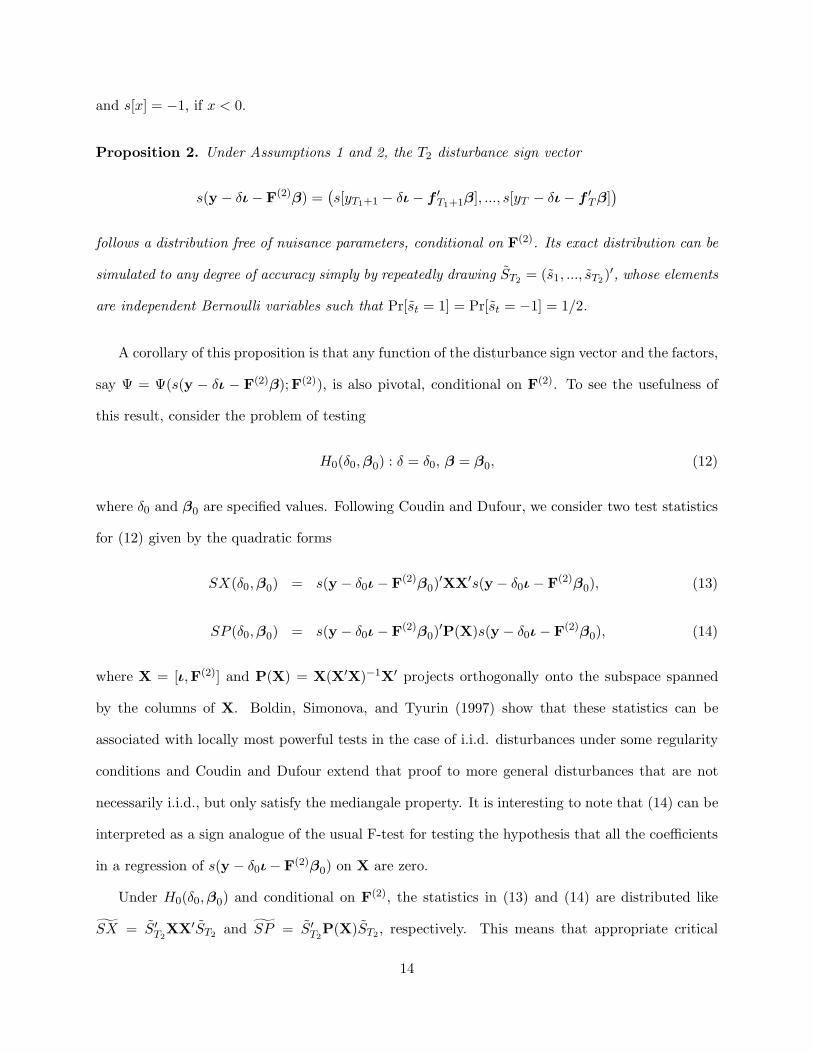
Proposition 2. Under Assumptions 1 and 2, the T2 disturbance sign vector

s(y − δι− F(2)β) =(s[yT1+1 − δι − f ′

T1+1β], ..., s[yT − δι− f ′Tβ]

)

follows a distribution free of nuisance parameters, conditional on F(2). Its exact distribution can be

simulated to any degree of accuracy simply by repeatedly drawing ST2= (s1, ..., sT2

)′, whose elements

are independent Bernoulli variables such that Pr[st = 1] = Pr[st = −1] = 1/2.

A corollary of this proposition is that any function of the disturbance sign vector and the factors,

say Ψ = Ψ(s(y − δι − F(2)β);F(2)), is also pivotal, conditional on F(2). To see the usefulness of

this result, consider the problem of testing

H0(δ0,β0) : δ = δ0, β = β0, (12)

where δ0 and β0 are specified values. Following Coudin and Dufour, we consider two test statistics

for (12) given by the quadratic forms

SX(δ0,β0) = s(y − δ0ι− F(2)β0)′XX′s(y− δ0ι− F(2)β0), (13)

SP (δ0,β0) = s(y − δ0ι− F(2)β0)′P(X)s(y − δ0ι− F(2)β0), (14)

where X = [ι,F(2)] and P(X) = X(X′X)−1X′ projects orthogonally onto the subspace spanned

by the columns of X. Boldin, Simonova, and Tyurin (1997) show that these statistics can be

associated with locally most powerful tests in the case of i.i.d. disturbances under some regularity

conditions and Coudin and Dufour extend that proof to more general disturbances that are not

necessarily i.i.d., but only satisfy the mediangale property. It is interesting to note that (14) can be

interpreted as a sign analogue of the usual F-test for testing the hypothesis that all the coefficients

in a regression of s(y − δ0ι− F(2)β0) on X are zero.

Under H0(δ0,β0) and conditional on F(2), the statistics in (13) and (14) are distributed like

SX = S′T2XX′ST2

and SP = S′T2P(X)ST2

, respectively. This means that appropriate critical

14

values from the conditional distributions may be found to obtain finite-sample tests of H0(δ0,β0).

For instance, consider the statistic in (14). The decision rule is then to reject H0(δ0,β0) at level

α if SP (δ0,β0) is greater than the (1 − α)-quantile of the distribution obtained by simulating

SP , say cSPα . A critical value cSXα can be found in similar fashion by simulating values SX .

When (13) and (14) are evaluated at the true parameter values (δ,β), Proposition 2 implies that

Pr[SX(δ,β) > cSXα ] = α and Pr[SP (δ,β) > cSPα ] = α as well. So for all 0 < α < 1, the critical

regions SX(δ0,β0) > cSXα and SP (δ0,β0) > cSPα each have size α.7 Note also that the critical

values cSXα and cSPα only need to be computed once, since they do not depend on δ0, β0.

Here the value of interest is δ0 = 0 which means that we are dealing with point null hypotheses

of the form

H0(β0) : δ = 0, β = β0, (15)

where β0 ∈ B, an admissible parameter space. The null hypothesis implied by (3) that we wish to

test is

H0 :⋃

β0∈B

H0(β0), (16)

the union of (15) taken over B. The expression in (16) makes clear that the elements of β are

nuisance parameters in this setting, since they are not constrained to a single value under the

null hypothesis. In order to test such a hypothesis, Dufour (2006) suggests a minimax argument

as in Savin (1984) which may be stated as “reject the null whenever for all admissible values of

the nuisance parameters under the null, the corresponding point null hypothesis is rejected;” see

also Jouneau-Sion and Torres (2006) for an application of this argument in a different context. In

general, Dufour’s rule in practice consists of maximizing the p-value of the sample test statistic

over the set of nuisance parameters. Given the present framework, this rule amounts to minimizing

the values of the SX and SP statistics over B. To see why, define

SXL = infβ0∈B

SX(0,β0) and SPL = infβ0∈B

SP (0,β0), (17)

7Following the terminology in Lehmann and Romano (2005, Chapter 3), we say that a test of H0 has size α if

Pr[Rejecting H0 |H0 true] = α, and that it has level α if Pr[Rejecting H0 |H0 true] ≤ α.

15

and observe that under H0 in (16) we have

0 ≤ SPL ≤ SP (0,β),

which shows that SPL is boundedly pivotal. This property further implies under H0 that

Pr[SPL > cSPα ] ≤ Pr[SP (0,β) > cSPα ] = α.

In other words, the test that rejects the null hypothesis H0 whenever SPL > cSPα has level α. The

same argument applies to (13) to get the critical region SXL > cSXα .

Here we compute SXL and SPL in (17) by searching over a grid B(β) specified around LAD

point estimates β, which are computed in the restricted (i.e. no intercept) median regression model

y = F(2)β + u. Of course, more sophisticated optimization methods such as simulated annealing

could be used to find SXL and SPL. The advantage of the naive grid search is that it is completely

reliable and feasible when the dimension of β is not too large. An important remark is that the

search for SXL and SPL can be stopped and the null hypothesis can no longer be rejected at level

α as soon as a grid point yields a non-rejection. At that point, values of β have been found that

make the model compatible with the data, meaning the model should not be rejected. For instance,

if SP (0, β) ≤ cSPα then SPL does not reject either and H0 in (16) is not significant at level α.

3.4 Summary of test procedure

Suppose that one wishes to use the SPL statistic in (17). In a preliminary step, the reference

distribution for that statistic is simulated to the desired degree of accuracy by generating a large

number, say M , of simulated i.i.d. values SP 1, ..., SPM and the α-level critical value cSPα is deter-

mined from the simulated distribution. The rest of the test procedure then proceeds according to

the following steps:

1. Compute the estimates ai of ai, for i = 1, ..., N , using the first T1 observations on rt and ft.

2. Compute the weights ωi, for i = 1, ..., N , according to:

ωi = sign(ai)1

N,

16

and then compute T2 portfolio returns as yt =∑N

i=1 ωirit, t = T1 + 1, ..., T .

3. Find SPL = infβ0∈B SP (0,β0).

4. Reject the null hypothesis H0 : a = 0 at level α if SPL > cSPα , or equivalently in terms of the

p-value if p(SPL) ≤ α. Here the p-value can be computed as

p(SPL) =1

M

M∑

j=1

I[SP j > SPL],

where I[A] is the indicator function of event A.

This procedure yields a finite-sample and distribution-free test of H0 in (3) over the class of all

disturbance distributions satisfying Assumption 1.

4 Simulation evidence

We present the results of some simulation experiments to compare the performance of the proposed

test procedure with several standard tests. The first of the benchmarks for comparison purposes

is the GRS test in (7). The other benchmarks are the usual LR test, an adjusted LR test, and a

test based on GMM. The latter is a particularly important benchmark here, since in principle it is

“robust” to non-normality and heteroskedasticity of returns.

The LR test is based on a comparison of the constrained and unconstrained log-likelihood

functions evaluated at the maximum likelihood estimates. The unconstrained estimates are given

in (4), (5), and (6). For the constrained case, the maximum likelihood estimates are

B∗ =

[T∑

t=1

rtf′t

] [T∑

t=1

ftf′t

]−1

,

Σ∗ =1

T

T∑

t=1

(rt − B∗ft

)(rt − B∗ft

)′

.

The LR test statistic, J2, is then given by

J2 = T[log |Σ∗| − log |Σ|

],

17

which, under the null hypothesis, follows an asymptotic chi-square distribution with N degrees

of freedom, χ2N . As we shall see, the finite sample behavior of J2 can differ vastly from what

asymptotic theory predicts. Jobson and Korkie (1982) suggest an adjustment to J2 in order to

improve its finite-sample size properties when used with critical values from the χ2N distribution.

The adjusted LR statistic is

J3 =T − (N/2) −K − 1

TJ2,

which also follows the asymptotic χ2N distribution, under H0.

MacKinlay and Richardson (1991) develop tests of mean-variance efficiency in a GMM frame-

work. For the asset pricing model in (1), the GMM tests are based on the moments of the following

(K + 1)N × 1 vector:

gt(θ) =

1

ft

⊗ εt(θ), (18)

where εt(θ) = rt−a−Bft. The symbol ⊗ refers to the Kronecker product. Here θ = (a′, vec(B)′)′,

where vec(B) is an NK×1 vector obtained by stacking the columns of B, one below the other, with

the columns ordered from left to right. The model specification in (1) implies the moment conditions

E(gt(θ0)) = 0, where θ0 is the true parameter vector. The system in (18) is exactly identified which

implies that the GMM procedure yields the same estimates of θ as does OLS applied equation

by equation. The covariance matrix of the GMM estimator θ is given by V = [D′0S

−10 D0]

−1,

where D0 = E[∂gT (θ)/∂θ′] with gT (θ) = T−1

∑Tt=1 gt(θ) and S0 =

∑+∞s=−∞E[gt(θ)gt−s(θ)

′]; see

Campbell, Lo, and MacKinlay (1997, Chapter 5). The GMM-based Wald test statistic is

J4 = T a′[R

(D−1S(D′)−1

)R′

]−1a, (19)

where D and S are consistent estimators of D0 and S0, respectively, and R = (1,0K) ⊗ IN , with

0K denoting a row vector of K zeros and IN as the N ×N identity matrix. Under H0, the statistic

J4 follows the χ2N distribution asymptotically.

We examine cases with K = 1 and K = 3 in model (1). For convenience, the three-factor

18

specification we consider is given again here as

rit = ai + bi1f1t + bi2f2t + bi3f3t + εit, t = 1, ..., T, i = 1, ..., N, (20)

with common factor returns following independent stochastic volatility processes of the form:

fjt = exp(hjt/2)ǫjt with hjt = λjhj,t−1 + ξjt,

where the independent terms ǫjt and ξjt are both i.i.d. according to a standard normal distribution

and the persistence parameters λj are set to 0.5. For j = 1, .., 3, the bij ’s are randomly drawn from

a uniform distribution between 0.5 and 1.5. All the tests are conducted at the nominal 5% level

and critical values for SXL and SPL are determined using 10,000 simulations. In the experiments

we choose mispricing values a and set half the intercept values as ai = a and the other half as

ai = −a. We denote this in the tables as |ai| = a. The estimates of ai, i = 1, ..., N , in Step 1 are

found via LAD. Finally, there are 1000 replications in each experiment.

Consider first the single-factor model so bi2 and bi3 in (20) are zero, in which case the null

hypothesis is a test of the mean-variance efficiency of the given factor portfolio. In the application

of the test procedure, a choice needs to be made about where to split the sample. While this

choice has no effect on the level of the tests, it obviously matters for their power. We do not

have analytical results on how to split the sample, so we resort to simulations. Table 1 shows the

power of the test procedure applied with the SXL and SPL statistics for various values of T1/T ,

where |ai| = 0.20, 0.15, and 0.10. These values are well within the range found in our empirical

application, where the intercepts estimated with monthly stock returns range in values from -0.5

to 1.5. Here we set T = 60 and N = 100 and the disturbance terms εit are drawn randomly from

the standard normal distribution. As expected, the results show that for any given value of T1/T

the power increases as |ai| increases. Overall, the results suggest that no less that 30% and no

more than 50% of the time-series observations should be used as the first subsample in order to

maximize power. Accordingly, the testing strategy represented by T1 = 0.4T is pursued in the

remaining comparative experiments.

19

We also include in our comparisons two distribution-free tests proposed by Gungor and Luger

(2009) that are applicable in the single-factor case. The building block of those tests is

zit =

(ri,t+m

f1,t+m

−ritf1t

)×

(f1t − f1,t+m)

f1tf1,t+m

, (21)

defined for t = 1, ...,m, where m = T/2 is assumed to be an integer. The first test is based on the

sign statistic

Si =

∑mt=1 0.5(s[zit] + 1)−m/2√

m/4(22)

and the second one is based the Wilcoxon signed rank statistic

Wi =

∑mt=1 0.5(s[zit] + 1)Rank(|zit|)−m(m+ 1)/4√

m(m+ 1)(2m+ 1)/24, (23)

where Rank(|zit|) is the rank of |zit| when |zi1|, ..., |zim| are placed in ascending order of magnitude.

Gungor and Luger (2009) show that a time-series symmetry condition ensures that both (22) and

(23) have limiting (as m → ∞) standard normal distributions. Under the further assumption that

the disturbance terms are cross-sectionally independent, conditional on (f11, ..., f1T )′, the sum-type

statistics

SD =N∑

i=1

S2i and WD =

N∑

i=1

W 2i (24)

follow an asymptotic chi-square distribution with N degrees of freedom. Simulation results show

that this approximation works extremely well and just like the test procedure proposed here, the

SD and WD test statistics can be calculated even if N is large.

Tables 2–5 show the empirical size (Panel A) and power (Panel B) of the considered tests when

|ai| = 0.15 and T = 60, 120 and N takes on values between 10 and 500. When they don’t respect the

nominal level constraint, the power results for the J tests are based on size-corrected critical values.

It is important to emphasize that size-corrected tests are not feasible in practice, especially under

the very general symmetry condition in Assumption 1. They are merely used here as theoretical

benchmarks for the truly distribution-free tests. In particular, we wish to see how the power of the

new tests compares to these benchmarks as T and N vary.

20

The results in Table 2 correspond to the single-factor model where the disturbance terms εit

are i.i.d. in both the time-series and the cross-section according to a standard normal distribution.

Here the parametric J1 behaves according to its distributional theory and the distribution-free

SD and WD tests also behave well under the null with empirical rejection rates close to the

nominal level. From Table 2, the conservative SXL and SPL tests are also seen to satisfy the level

constraint in the sense that the probability of a Type I error remains bounded by the nominal level

of significance. The J2, J3, and J4 tests, however, suffer massive size distortions as the number of

equations increases.8 When T = 120 and N = 100, the LR test (J2) rejects the true null with an

empirical probability of 100% and in the case of the adjusted LR test (J3) that probability is still

above 50%. Notice also that the J tests are not computable when N exceeds T . Such cases are

indicated with “-” in the tables.

In Panel B of Table 2, we see the same phenomenon as in Figure 1: for a fixed T , the power of

the GRS J1 test rises and then eventually drops as N keeps on increasing. Note that J1, J2, and

J3 have identical size-corrected powers, since they are all related via monotonic transformations

(Campbell, Lo, and MacKinlay 1997, Ch. 5). On the contrary, the power of the SD and WD tests

and that of the new SXL and SPL tests increases monotonically with N .

The next specification we consider resembles a stochastic volatility model and introduces depen-

dence between the conditional covariance matrix and f1t. Specifically, we let εit = exp(λif1t/2)ηit,

where the innovations ηit are standard normal and the λi’s are randomly drawn from a uniform

distribution between 1.5 and 2.5. It should be noted that such a contemporaneous heteroskedastic

specification finds empirical support in Duffee (1995, 2001) and it is easy to see that it generates

εit’s with time-varying excess kurtosis—a well-known feature of asset returns. Panel A of Table

3 reveals that all the parametric tests have massive size distortions in this case, and these over-

rejections worsen as N increases for a given T .9 When T = 120, the J tests all have empirical sizes

8This overrejection problem with standard asymptotic tests in multivariate regression models is also documented

in Stambaugh (1982), Jobson and Korkie (1982), Amsler and Schmidt (1985), MacKinlay (1987), Stewart (1997),

and Dufour and Khalaf (2002).9The sensitivity of the GRS test to contemporaneous heteroskedasticity is also documented in MacKinlay and

21

around 20%. The probability of a Type I error for all those tests exceeds 65% when N is increased

to 50. In sharp contrast, the four distribution-free tests satisfy the nominal 5% level constraint, no

matter T and N . As in the first example, Panel B shows the power of the distribution-free tests

increasing with both T and N in this heteroskedastic case.

At this point, one may wonder what is the advantage of the new SXL and SPL tests over the

SD and WD tests of Gungor and Luger (2009) since the latter display better power in Panel B

of Tables 2 and 3. Those tests achieve higher power because they eliminate the bi1’s from the

inference problem through the long differences in (21), whereas the new tests proceed through a

minimization of the test statistics over the intervening nuisance parameter space. A limitation

of the SD and WD tests, however, is that they are valid only under the assumption that the

model disturbances are cross-sectionally independent. Table 4 reports the empirical size of the

those tests when the cross-sectional disturbances inherit a common factor structure. Namely, we

let εit = γiwt + eit, where the common factor wt and the idiosyncratic term eit are independent

and both i.i.d. according to a standard normal distribution. The factor loadings γi are drawn from

a uniform distribution over the interval [0, Umax] and Umax is varied between 0.5 and 2.0. The

nominal level is 0.05 and we consider T = 60, 120 and N = 10, 100. We see from Table 4 that the

SD and WD tests are fairly robust to mild cross-sectional correlation, but start over-rejecting as

the cross-sectional dependence increases and this problem is further exacerbated when N increases.

As expected, Table 4 shows that SXL and SPL are not affected by cross-sectional dependence.

Table 5 reports the results for the three-factor model, as given in (20). The disturbance terms are

governed by εit = exp(λif∗t /2)ηit like in the case of Table 3, except that now f∗

t = (f1t+f2t+f3t)/3

so all three factors contribute (equally) to the variance heterogeneity. Note that the SD and WD

statistics in (24) are not computable in the presence of multiple factors. Table 5 echoes the previous

findings for the J tests about their size distortions and decreasing power as N increases. What’s

new in Table 5 is that the SXL and SPL tests appear to be more conservative in this case, so N

needs to be increased in order to attain the power levels seen in Tables 2 and 3. In the empirical

Richardson (1991), Zhou (1993), and Gungor and Luger (2009).

22

illustration that follows, we apply the new tests with N = 10, 100, and 503 test assets.

5 Empirical illustration

In this section we illustrate the new tests with two empirical applications. First, we examine the

Sharpe-Lintner version of the CAPM. This single-factor model uses the excess returns of a value-

weighted stock market index of all stocks listed on the NYSE, AMEX, and NASDAQ. Second, we

test the more general three-factor model of Fama and French (1993), which adds two factors to the

CAPM specification: (i) the average returns on three small market capitalization portfolios minus

the average return on three big market capitalization portfolios, and (ii) the average return on two

value portfolios minus the average return on two growth portfolios. Note that the CAPM is nested

within the Fama-French model. This means that if there was no sampling uncertainty, finding that

the market portfolio is mean-variance efficient would trivially imply the validity of the three-factor

model. Conversely, if the three-factor model does not hold, then the CAPM is also rejected.

We test both specifications with three sets of test assets comprising the stocks traded on the

NYSE, AMEX, and NASDAQ markets for the 38-year period from January 1973 to December 2010

(456 months). The first two data sets are the monthly returns on 10 portfolios formed on size, and

100 portfolios formed on both size and the book-to-market ratio. Those two data sets are available

in Ken French’s online data library. The third data set we make use of comprises the returns on

503 individual stocks traded on the markets mentioned above. These represent all the stocks for

which there is data in the Center for Research in Security Prices (CRSP) monthly stock files for

the entire 38-year sample period. The complete list of company names is given in the appendix.

Finally, we use the one-month U.S. Treasury bill as the risk-free asset.

Figure 2 plots the excess returns of the stock market index over the full sample period. That

figure shows that this typical return series contains several extreme observations. For instance, the

returns seen during the stock market crash of October 1987, the financial crisis of 2008, and at

some other points in time as well are obviously not representative of normal market activity; we

23

discuss the effects of extreme observations in Section 5.4. It is also quite common in the empirical

finance literature to perform asset pricing tests over subperiods out of concerns about parameter

stability. So in addition to the entire 38-year period, we also examine six 5-year, one 8-year, and

three 10-year subperiods. For other examples of this practice, see Campbell, Lo, and MacKinlay

(1997), Gungor and Luger (2009), and Ray, Savin, and Tiwari (2009).

5.1 10 size portfolios

Table 6 reports the CAPM test results based on the ten size portfolios. The numbers reported in

parenthesis are p-values and the entries in bold represent cases of significance at the 5% level. We

see here that the parametric J tests reject the null hypothesis over the entire sample period with

p-values no more than 5%. The non-parametric SD and WD tests also indicate strong rejections.

In contrast, the SXL and SPL tests clearly do not reject the mean-variance efficiency of the market

index.

Looking at the subperiods, we see that the only rejection by the new tests occurs with SPL in

the 10-year subperiod 1/73–12/82. In the 5-year subperiod 1/98–12/02, the J2 and J4 tests reject

the CAPM specification. The results for the J tests during the last 10-year subperiod from 1/93 to

12/02 agree with the rejection findings for the entire sample period. Besides the obvious differences

between the parametric and non-parametric inference results, Table 6 also reveals some differences

between the SD and WD tests and the proposed SXL and SPL tests. One possible reason for the

disagreement across these non-parametric tests could be the presence of cross-sectional disturbance

correlations. As we saw in Table 4, the SD and WD tests are not robust to such correlations,

whereas the new tests allow for cross-sectional dependencies just like the GRS test.

Table 7 shows the results for the Fama-French model. For the entire 38-year sample period, the

results in Table 7 are in line with those for the single-factor model in Table 6. The standard J tests

reject the null with very low p-values, whereas the distribution-free SXL and SPL tests are not

significant. In the 5-year subperiods, we see some disagreements among the parametric tests. For

instance, during 1/98–12/02 the J1 and J3 indicate non-rejections, while J2 and J4 point toward

24

rejections of the null. The results for the last two 10-year subperiods resemble those for the entire

sample period and the J tests depict a more consistent picture.

Table 7 shows that the SXL and SPL tests never reject the three-factor specification. Taken

at face value, these results would suggest that the excess returns of the 10 size portfolios are well

explained by the three Fama-French factors. This is entirely consistent with the non-rejections seen

in Table 6 and it suggests that the size and the book-to-market factors play no role; i.e., the CAPM

factor alone can price the 10 size portfolios.

Upon observing that the Fama-French model is never rejected by the non-parametric SXL and

SPL tests with 10 test assets, one may be concerned about the ability of the new procedure to reject

the null, when the alternative is true. In order to boost power, we proceed next with a tenfold

increase in the number of test assets.

5.2 100 size and book-to-market portfolios

Tables 8 and 9 show the test results for the two considered factor specifications using return data on

100 portfolios formed on size and book-to-market. Note that with N = 100, none of the parametric

tests are computable in the 5-year subperiods where T = 60.

Using the entire sample, the J tests decisively reject both factor specifications. In the single-

factor case (Table 8), the inference results based on the SD andWD tests are in agreement with the

parametric ones. Note again that the SD and WD tests cannot be computed in the three-factor

specification (Table 9). The interesting result in Tables 8 and 9 is that the SPL also indicates

rejections. Compared to Tables 6 and 7, it would seem that increasing N from 10 to 100 delivered

more power, at least for the entire sample period. Rejections are also seen for SPL in the last

10-year subperiod.

The rejections by the SPL test seen in Tables 8 and 9 with N = 100 beg the question: what

would happen if N was increased even further? To answer that question, we turn next to the

individual stock data.

25

5.3 503 individual stocks

Tables 10 and 11 report the test results using the returns on 503 individual stocks. Here the J

tests cannot be computed, since N > T . The most striking result is that now for the entire sample

period (T = 456) the preferred SPL test no longer indicates a rejection of either the CAPM nor

the Fama-French three-factor model. This stands in sharp contrast to the results seen in Tables 8

and 9 with 100 portfolio returns. The results in Tables 8 and 10 from the SD and WD tests also

agree with the non-rejection of the CAPM when moving from portfolios to individual stocks.

These results suggest that the excess returns on individual stocks are well explained by the

CAPM, which in turn suggests that the size and the book-to-market factors play no role in pricing

this collection of assets. It also appears that creating portfolios on the basis of size and book-

to-market biases the test outcomes toward a rejection of the model’s validity. This finding with

the newly proposed SPL test is entirely consistent with the analysis in Lo and MacKinlay (2000),

who show that sorting stocks into groups based on variables that are correlated with returns is a

questionable practice since it favors a rejection of the asset pricing model under consideration; see

also Berk (2000) for related theoretical analysis. Finally, it is interesting to note that this conclusion

about the validity of the CAPM is also reached by Zhou (1993), Vorkink (2003), Gungor and Luger

(2009), and Ray, Savin, and Tiwari (2009).

5.4 Extreme observations

Looking back upon the results in Tables 6 and 7 with 10 size portfolios, one might think that

the differences between the parametric J tests and the SXL and SPL tests is due to a lack of

power by the latter when N is small. However, another plausible reason for these differences is

the adverse effect that a small number of extreme observations can have on the OLS estimates

used to compute the J tests; see Vorkink (2003). To investigate that possibility we recompute the

parametric tests with winsorized data. This procedure has the effect of decreasing the magnitude

of extreme observations but leaves them as important points in the sample.

26

Table 12 shows the results of the J tests with the 10 size portfolios when the full-sample returns

are winsorized at the 0.3%, 0.5%, 0.7%, and 1% levels. In the single-factor case (Panel A), the J

tests cease to be significant at the 5% level with returns winsorized at 0.3%. For the three-factor

model (Panel B), the same pattern of increasing p-values occurs across winsorization levels. These

results clearly show that OLS-based inference can be very sensitive to the presence of even just a

few extreme observations.

6 Conclusion

The beta-pricing representation of linear factor pricing models is typically assessed with tests based

on OLS or GMM. In this context, standard asymptotic theory is known to provide a poor approx-

imation to the finite-sample distribution of those test statistics, even with fairly large samples. In

particular, the asymptotic tests tend to over-reject the null hypothesis when in fact it is true, and

these size distortions grow quickly as the number of included test assets increases. So the conclu-

sions of empirical studies that adopt such procedures can lead one to spuriously reject the validity

of the asset pricing model.

Exact finite-sample methods that avoid the spurious rejection problem usually rely on strong

distributional assumptions about the model’s disturbance terms. A prominent example is the GRS

test that assumes that the disturbance terms are identically distributed each period according

to a multivariate normal distribution. Yet it is known from the empirical finance literature that

financial asset returns are non-normal, exhibiting time-varying covariance structures and excess

kurtosis. These stylized facts would put into question the reliability of any inference method that

assumes that the cross-sectional distribution of disturbance terms is homogenous over time.

Another serious problem with standard inference methods has to do with the choice of how

many tests assets to include. Indeed, if too many are included relative to the number of available

time-series observations, the GRS test may lose all its power or may not even be computable. In

fact, any procedure that relies on unrestricted estimates of the covariance matrix of regression

27

disturbances will no longer be computable owing to the singularity that occurs when the size of the

cross-section exceeds the length of the time series.

In this paper we have proposed a finite-sample test procedure that overcomes these problems.

Specifically, our statistical framework makes no parametric assumptions about the distribution

of the disturbance terms in the factor model. The only requirement is that the cross-section

disturbance vectors be independent over time, conditional on the factors, and reflectively symmetric

each period. The class of reflectively symmetric distributions includes elliptically symmetric ones,

which are theoretically consistent with mean-variance analysis. Our non-parametric framework

leaves open the possibility of unknown forms of time-varying non-normalities and many other

distribution heterogeneities, such as time-varying covariance structures, time-varying kurtosis, etc.

The procedure is an adaptive one that first splits the sample to combine the assets into a sin-

gle portfolio using weights based on the sign of estimated regression intercepts from a subsample.

This solves the problem of too many assets and could of course be used in conjunction with an

assumed parametric form of the multivariate disturbance distribution. The Lehmann and Stein

(1949) impossibility theorem, however, shows that if we wish to remain completely agnostic about

heteroskedasticity, then the only valid tests are those based on sign statistics. Even though some

studies such as Affleck-Graves and McDonald (1989) report evidence showing the GRS test to

be fairly robust to (some specified) deviations from normality, we find it hard to have faith in a

parametric procedure whose assumptions are so obviously at odds with the empirical evidence.

Moreover our results show that the power of the new sign-based test procedure increases as either

the time-series lengthens and/or the cross-section becomes larger. So the truly robust inference pro-

cedure developed here offers a very compelling way to assess linear factor pricing models, especially

with a large number of test assets.

28

References

Affleck-Graves, J. and B. McDonald. 1989. “Nonnormalities and tests of asset pricing theories.”

Journal of Finance 44: 889–908.

Amsler, C.E. and P. Schmidt. 1985. “A Monte Carlo investigation of the accuracy of multivariate

CAPM tests.” Journal of Financial Economics 14: 359–375.

Bassett G. and R. Koenker. 1978. “Asymptotic theory of least absolute error regression.” Journal

of the American Statistical Association 73: 618–622.

Beaulieu, M.-C., Dufour, J.-M. and L. Khalaf. 2007. “Multivariate tests of mean-variance effi-

ciency with possibly non-Gaussian errors.” Journal of Business and Economic Statistics 25:

398-410.

Behboodian, J. 1990. “Some characterization theorems on symmetry.” Computational Statistics

and Data Analysis 10: 189–192.

Berk, J. 1997. “Necessary conditions for the CAPM.” Journal of Economic Theory 73: 245–257.

Berk, J. 2000. “Sorting out sorts.” Journal of Finance 55: 407–427.

Blattberg, R. and N. Gonedes. 1974. “A comparison of the stable and student distributions as

statistical models of stock prices.” Journal of Business 47: 244–280.

Boldin, M.V., Simonova, G.I. and Y.N. Tyurin. 1997. Sign-based methods in Linear Statistical

Models. American Mathematical Society, Maryland.

Bossaerts, P. and P. Hillion. 1995. “Testing the mean-variance efficiency of well-diversified port-

folios in very large cross-sections.” Annales d’Economie et de Statistique 40: 93–124.

Breeden, D.T. 1979. “An intertemporal asset pricing model with stochastic consumption and

investment opportunities.” Journal of Financial Economics 7: 265–296.

29

Campbell, J.Y., A.W. Lo, and A.C. MacKinlay. 1997. The Econometrics of Financial Markets.

Princeton University Press, New Jersey.

Chamberlain, G. 1983. “A characterization of the distributions that imply mean-variance utility

functions.” Journal of Economic Theory 29: 185–201.

Chou, P.-H. and G. Zhou. 2006. “Using bootstrap to test portfolio efficiency.” Annals of Eco-

nomics and Finance 1: 217–249.

Coudin, E. and J.-M. Dufour. 2009. “Finite-sample distribution-free inference in linear median

regressions under heteroscedasticity and non-linear dependence of unknown form.” Econo-

metrics Journal 12: 19–49.

DeMiguel, V., L. Garlappi, and R. Uppal. 2009. “Optimal versus naive diversification: how

inefficient is the 1/N portfolio strategy?” Review of Financial Studies 22: 1915–53.

Duffee, G.R. 1995. “Stock returns and volatility: a firm-level analysis.” Journal of Financial

Economics 37: 399–420.

Duffee, G.R. 2001. “Asymmetric cross-sectional dispersion in stock returns: evidence and impli-

cations.” Federal Reserve Bank of San Francisco Working Paper No. 2000-18.

Dufour, J.-M. 2003. “Identification, weak instruments, and statistical inference in econometrics.”

Canadian Journal of Economics 36: 767–808.

Dufour, J.-M. 2006. “Monte Carlo tests with nuisance parameters: A general approach to finite-

sample inference and nonstandard asymptotics.” Journal of Econometrics 133: 443–477.

Dufour, J.-M. and M. Hallin. 1991. “Nonuniform bounds for nonparametric t tests.” Econometric

Theory 7: 253–263.

Dufour, J.-M. and L. Khalaf. 2002. “Simulation-based finite- and large-sample tests in multivari-

ate regressions.” Journal of Econometrics 111: 303–322.

30

Dufour, J.-M. and M. Taamouti. 2005. “Projection-based statistical inference in linear structural

models with possibly weak instruments.” Econometrica 73: 1351–1365.

Dufour, J.-M. and A. Taamouti. 2010. “Exact optimal inference in regression models under

heteroskedasticity and non-normality of unknown form.” Computational Statistics and Data

Analysis 54: 2532–2553.

Fama, E. 1965. “The behavior of stock market prices.” Journal of Business 38: 34–105.

Fama, E.F. and K.R. French. 1993. “Common risk factors in the returns on stocks and bonds.”

Journal of Financial Economics 33: 3–56.

Fama, E.F. and J.D. MacBeth. 1973. “Risk, return, and equilibrium: empirical tests.” Journal

of Political Economy 81: 607–636.

Ferson, W.E. and S.R. Foerster. 1994. “Finite sample properties of the Generalized Method of

Moments in tests of conditional asset pricing models.” Journal of Financial Economics 36:

29–55.

Gibbons, M.R., Ross, S.A. and J. Shanken. 1989. “A test of the efficiency of a given portfolio.”

Econometrica 57: 1121–1152.

Glahe, F.R. and J.F. Hunt. 1970. “The small sample properties of simultaneous equation least

absolute estimators vis-a-vis least squares estimators.” Econometrica 38: 742–753.

Grinblatt, M. and S. Titman. 1987. “The relation between mean-variance efficiency and arbitrage

pricing.” Journal of Business 60: 97–112.

Gungor, S. and R. Luger. 2009. “Exact distribution-free tests of mean-variance efficiency.” Jour-

nal of Empirical Finance 16: 816–829.

Harvey, C.R. and G. Zhou. 1990. “Bayesian inference in asset pricing tests.” Journal of Financial

Economics 26: 221–254.

31

Hsu, D.A. 1982. “A Bayesian robust detection of shift in the risk structure of stock market

returns.” Journal of the American Statistical Association 77: 29–39.

Huberman, G., Kandel, S. and R.F. Stambaugh. 1987. “Mimicking portfolios and exact arbitrage

pricing.” Journal of Finance 42: 1–9.

Hunt, J.G., Dowling, J.M. and F.R. Glahe. 1974. “L1 estimation in small samples with Laplace

error distributions.” Decision Sciences 5: 22–29.

Jagannathan, R. and T. Ma. 2003. “Risk reduction in large portfolios: why imposing the wrong

constraints helps.” Journal of Finance 58: 1651–1684.

Jobson, J.D. 1982. “A multivariate linear regression test for the Arbitrage Pricing Theory.”

Journal of Finance 37: 1037–1042 .

Jobson, J.D. and B. Korkie. 1982. “Potential performance and tests of portfolio efficiency.”

Journal of Financial Economics 10: 433–466.

Jobson, J.D. and B. Korkie. 1985. “Some tests of linear asset pricing with multivariate normality.”

Canadian Journal of Administrative Sciences 2: 114–138.

Jouneau-Sion, F. and O. Torres. 2006. “MMC techniques for limited dependent variables models:

Implementation by the branch-and-bound algorithm.” Journal of Econometrics 133: 479–512.

Kandel, S., McCulloch, R. and R.F. Stambaugh. 1995. “Bayesian inference and portfolio effi-

ciency.” Review of Financial Studies 8: 1–53.

Kocherlakota, N.R. 1997. “Testing the Consumption CAPM with heavy-tailed pricing errors.”

Macroeconomic Dynamics 1: 551–567.

Ledoit, O. and M. Wolf. 2003. “Improved estimation of the covariance matrix of stock returns

with an application to portfolio selection.” Journal of Empirical Finance 10: 603–621.

32

Ledoit, O. and M. Wolf. 2004. “Honey, I shrunk the sample covariance matrix.” Journal of

Portfolio Management 30: 110–119.

Lehmann, E.L. and J.P. Romano. 2005. Testing Statistical Hypotheses, Third Edition. Springer,

New York.

Lehmann, E.L. and C. Stein. 1949. “On the theory of some non-parametric hypotheses.” Annals

of Mathematical Statistics 20: 28–45.

Lintner, J. 1965. “The valuation of risk assets and the selection of risky investments in stock

portfolios and capital budgets.” Review of Economics and Statistics 47: 13–37.

Lo, A. and A.C. MacKinlay. 1990. “Data-snooping biases in tests of financial asset pricing

models.” Review of Financial Studies 3: 431–467.

MacKinlay, A.C. 1987. “On multivariate tests of the Capital Asset Pricing Model.” Journal of

Financial Economics 18: 341–372.

MacKinlay, A.C. and M.P. Richardson. 1991. “Using Generalized Method of Moments to test

mean-variance efficiency.” Journal of Finance 46: 511–527.

Merton, R.C. 1973. “An intertemporal capital asset pricing model.” Econometrica 41: 867–887.

Michaud, R. 1989. “The Markowitz optimization enigma: is ‘optimized’ optimal?” Financial

Analysts Journal 45: 31–42.

Mitra, A. 1987. “Minimum absolute deviation estimation in regression analysis.” Computers and

Industrial Engineering 12: 67–76.

Neuhaus, G. and L.-X. Zhu. 1999. “Permutation tests for multivariate location problems.” Jour-

nal of Multivariate Analysis 69: 167–192.

Newey, W.K. and K.D. West. 1987. “A simple, positive semi-definite, heteroskedasticity and

autocorrelation consistent covariance matrix.” Econometrica 55: 703–708.

33

Owen, J. and R. Rabinovitch. 1983. “On the class of elliptical distributions and their applications

to the theory of portfolio choice.” Journal of Finance 38: 745–752.

Pfaffenberger, R.C. and J.J. Dinkel. 1978. “Absolute deviations curve fitting: an alternative to

least squares.” In Contributions to Survey Sampling and Applied Statistics (H.A. David, ed.)

Academic Press, New York.

Pratt, J.W. and J.D. Gibbons. 1981. Concepts of Nonparametric Theory. Springer, New York.

Ray, S., Savin, N.E. and A. Tiwari. 2009. “Testing the CAPM revisited.” Journal of Empirical

Finance 16: 721–733.

Roll, R. 1979. “A reply to Mayers and Rice (1979).” Journal of Financial Economics 7: 391–400.

Rosenberg, B. and D. Carlson. 1977. “A simple approximation of the sampling distribution of

least absolute residuals regression estimates.” Communications in Statistics - Simulation and

Computation 6: 421–437.

Ross, S.A. 1976. “The arbitrage theory of capital asset pricing.” Journal of Economic Theory 13:

341–360.

Savin, N.E. 1984. Multiple hypothesis testing. In: Griliches, Z., Intriligator, M.D. (Eds.), Hand-

book of Econometrics, North-Holland, Amsterdam.

Sentana, E. 2009. “The econometrics of mean-variance efficiency tests: a survey.” Econometrics

Journal 12: 65–101.

Serfling, R.J. 2006. “Multivariate symmetry and asymmetry.” In Encyclopedia of Statistical

Sciences, Second Edition (S. Kotz, N. Balakrishnan, C. B. Read and B. Vidakovic, eds.),

Wiley.

Shanken, J. 1987. “A Bayesian approach to testing portfolio efficiency.” Journal of Financial

Economics 19: 195–216.

34

Shanken, J. 1996. “Statistical methods in tests of portfolio efficiency: a synthesis.” In Handbook

of Statistics, Vol. 14: Statistical Methods in Finance. (G.S. Maddala and C.R. Rao, eds.),

North-Holland, Amsterdam.

Sharpe, W.F. 1964. “Capital asset prices: a theory of market equilibrium under conditions of

risk.” Journal of Finance 19: 425–442.

Stambaugh, R.F. 1982. “On the exclusion of assets from tests of the two-parameter model: a

sensitivity analysis.” Journal of Financial Economics 10: 237–268.

Stewart, K.G. 1997. “Exact testing in multivariate regression.” Econometric Reviews 16: 321–352.

Vorkink, K. 2003. “Return distributions and improved tests of asset pricing models.” Review of

Financial Studies 16: 845–874.

White, H. 1980. “A heteroskedasticity-consistent covariance matrix estimator and a direct test

for heteroskedasticity.” Econometrica 48: 817–838.

Zhou, G. 1993. “Asset-pricing tests under alternative distributions.” Journal of Finance 48:

1927–1942.

35

Table 1

Empirical power comparisons for various sample splits

T1/T 0.2 0.3 0.4 0.5 0.6 0.7 0.8

|ai| = 0.20

SXL 77.9 84.0 88.4 81.2 73.7 52.9 9.5

SPL 89.5 94.2 97.4 96.8 94.6 81.8 34.4

|ai| = 0.15

SXL 31.3 36.2 38.0 34.3 32.0 17.9 2.6

SPL 48.4 54.2 58.7 55.7 53.5 34.4 9.4

|ai| = 0.10

SXL 4.6 5.0 6.0 5.1 3.5 2.1 0.2

SPL 9.4 10.2 12.3 10.0 8.2 4.3 1.7

Notes: This table reports the empirical power (in percentages) of the proposed test

procedure based on the SXL and SPL statistics in (17) for various sample splits,

T1/T . The sample size is T = 60 and the number of test assets is N = 100. The

returns are generated according to a single-factor model with i.i.d. disturbances

following a standard normal distribution. The notation |ai| = a means that N/2

pricing errors are set as ai = −a and the other half are set as ai = a. The nominal

level is 0.05 and the results are based on 1000 replications.

36

Table 2

Empirical size and power: 1-factor model with homoskedastic disturbances

T N J1 J2 J3 J4 SD WD SXL SPL

Panel A: Size

60 10 5.4 10.0 5.4 9.0 4.8 4.9 0.1 0.2

25 5.2 31.7 6.9 15.6 4.7 3.8 0.1 0.4

50 4.1 98.7 40.7 36.6 3.9 3.6 0.3 0.5

100 - - - - 5.0 4.6 0.2 0.3

125 - - - - 4.4 2.9 0.1 0.3

120 10 4.2 5.9 4.2 5.8 5.0 4.5 0.2 0.5

25 4.1 11.9 4.5 7.2 4.9 4.0 0.7 1.2

50 5.3 43.0 8.2 16.1 4.1 4.3 0.3 0.8

100 4.7 100.0 54.1 34.3 4.3 5.0 0.4 0.6

125 - - - - 4.5 4.8 0.5 0.9

Panel B: Size-corrected power

60 10 59.5 59.5 59.5 57.8 19.4 22.3 3.3 6.2

25 75.4 75.4 75.4 74.1 29.6 33.2 5.3 12.3

50 43.6 43.6 43.6 42.1 43.3 52.1 16.7 28.1

100 - - - - 70.6 79.0 38.0 58.7

125 - - - - 77.2 85.5 48.9 71.1

120 10 95.8 95.8 95.8 95.7 39.0 42.9 15.9 25.2

25 100.0 100.0 100.0 100.0 64.6 73.1 42.1 59.5

50 100.0 100.0 100.0 100.0 87.6 93.8 74.4 87.6

100 98.3 98.3 98.3 98.6 98.2 99.6 97.5 99.6

125 - - - - 99.5 99.8 99.4 100.0

Notes: This table reports the empirical size (Panel A) and size-corrected power (Panel B) of the GRS test (J1),

the LR test (J2), an adjusted LR test (J3), a GMM-based test (J4), a sign test (SD), a Wilcoxon signed rank

test (SD), and the proposed SXL and SPL tests. The returns are generated according to a single-factor model

with i.i.d. disturbances following a standard normal distribution. The pricing errors are zero under H0, whereas

N/2 pricing errors are set equal to −0.15 and the other half are set to 0.15 under H1. The nominal level is 0.05

and entries are percentage rates. The results are based on 1000 replications and the symbol “-” is used whenever

a test is not computable.

37

Table 3

Empirical size and power: 1-factor model with contemporaneous heteroskedasticity

T N J1 J2 J3 J4 SD WD SXL SPL

Panel A: Size

60 10 22.7 33.7 22.9 27.1 5.0 5.1 0.7 1.0

25 43.9 79.9 47.7 60.2 5.1 4.5 0.6 1.4

50 46.4 95.3 86.2 82.7 4.9 4.7 0.3 0.6

100 - - - - 4.8 4.3 0.3 1.1

200 - - - - 5.1 3.6 0.5 1.2

120 10 18.9 22.7 18.9 18.5 5.0 4.2 0.7 1.4

25 38.6 56.4 39.3 43.5 3.7 3.7 0.5 1.9

50 65.2 93.3 68.9 75.7 4.1 4.3 0.5 1.6

100 67.6 94.5 89.8 81.7 5.1 4.8 1.4 1.3

200 - - - - 4.0 3.9 1.5 1.7

Panel B: Size-corrected power

60 10 18.7 18.7 18.7 21.4 14.2 17.2 1.5 3.3

25 31.7 31.7 31.7 30.8 21.7 23.9 2.2 5.0

50 34.6 34.6 34.6 22.7 31.4 34.7 5.0 9.0

100 - - - - 50.8 58.5 10.3 15.4

200 - - - - 74.4 82.6 19.8 28.2

120 10 24.1 24.1 24.1 24.7 29.7 30.9 6.2 10.8

25 50.7 50.7 50.7 52.9 47.8 53.1 14.1 21.3

50 78.9 78.9 78.9 74.9 71.2 77.3 30.4 38.3

100 73.8 73.8 73.8 65.3 89.6 95.3 52.3 60.1

200 - - - - 99.0 99.6 78.6 84.1

Notes: This table reports the empirical size (Panel A) and size-corrected power (Panel B) of the GRS

test (J1), the LR test (J2), an adjusted LR test (J3), a GMM-based test (J4), a sign test (SD), a

Wilcoxon signed rank test (SD), and the proposed SXL and SPL tests. The returns are generated

according to a single-factor model with contemporaneous heteroskedastic disturbances. The pricing

errors are zero under H0, whereas N/2 pricing errors are set equal to −0.15 and the other half are set to

0.15 under H1. The nominal level is 0.05 and entries are percentage rates. The results are based on 1000

replications and the symbol “-” is used whenever a test is not computable.

38

Table 4

Empirical size under cross-sectional disturbance factor structure

N = 10 N = 100

Umax 0.5 1.0 1.5 2.0 0.5 1.0 1.5 2.0

T = 60

SD 5.9 6.2 7.6 9.0 7.6 13.7 18.4 20.3

WD 5.7 7.7 8.3 9.7 8.5 15.9 18.8 20.7

SXL 0.0 0.2 0.3 0.1 0.2 0.2 0.1 0.3

SPL 0.4 0.5 0.6 0.9 0.4 0.3 0.5 0.2

T = 120

SD 6.7 6.6 8.6 9.3 6.4 12.0 15.2 17.7

WD 6.1 7.1 8.7 8.9 6.5 13.2 15.7 17.8

SXL 0.2 0.1 0.2 0.4 0.2 0.2 0.3 0.1

SPL 0.7 0.5 0.5 0.8 0.2 0.9 0.4 0.7

Notes: This table reports the empirical size of a sign test (SD), a Wilcoxon signed rank

test (WD), and the proposed SXL and SPL tests when the 1-factor model cross-sectional

disturbances have a factor structure; the factor loadings are uniformly distributed over

[0, Umax]. The nominal level is 0.05 and entries are percentage rates. The results are

based on 1000 replications

39

Table 5

Empirical size and power: 3-factor model with contemporaneous heteroskedasticity

T N J1 J2 J3 J4 SD WD SXL SPL

Panel A: Size

60 25 30.2 66.9 34.3 57.2 - - 0.0 0.0

50 29.5 99.8 86.5 92.4 - - 0.0 0.1

100 - - - - - - 0.0 0.0

200 - - - - - - 0.0 0.0

500 - - - - - - 0.0 0.1

120 25 25.6 41.5 26.6 36.9 - - 0.0 0.3

50 49.4 89.3 55.8 72.7 - - 0.0 0.3

100 60.4 100.0 97.8 95.6 - - 0.2 0.8

200 - - - - - - 0.4 0.6

500 - - - - - - 1.8 2.4

Panel B: Size-corrected power

60 25 35.2 35.2 35.2 33.6 - - 0.0 0.2

50 24.1 24.1 24.1 23.8 - - 0.0 1.4

100 - - - - - - 0.3 3.9

200 - - - - - - 0.6 12.3

500 - - - - - - 5.9 43.7

120 25 72.7 72.7 72.7 80.2 - - 1.0 7.9

50 90.5 90.5 90.5 90.1 - - 7.2 19.4

100 81.9 81.9 81.9 69.0 - - 28.2 53.7

200 - - - - - - 65.8 88.6

500 - - - - - - 95.8 99.2

Notes: This table reports the empirical size (Panel A) and size-corrected power (Panel B) of the GRS

test (J1), the LR test (J2), an adjusted LR test (J3), a GMM-based test (J4), a sign test (SD), a

Wilcoxon signed rank test (SD), and the proposed SXL and SPL tests. The returns are generated

according to a 3-factor model with contemporaneous heteroskedastic disturbances. The pricing errors are

zero under H0, whereas N/2 pricing errors are set equal to −0.15 and the other half are set to 0.15 under

H1. The nominal level is 0.05 and entries are percentage rates. The results are based on 1000 replications

and the symbol “-” is used whenever a test is not computable.

40

Table 6

Tests of the CAPM with 10 size portfolios

Time period J1 J2 J3 J4 SD WD SXL SPL

38-year period

1/73–12/10 1.83 18.43 18.14 18.48 38.45 35.25 208.77 0.06(0.05) (0.05) (0.05) (0.04) (0.00) (0.00) (0.92) (0.97)

5-year subperiods and an 8-year subperiod

1/73–12/77 0.56 6.46 5.71 5.24 16.80 15.09 197.79 4.02(0.83) (0.77) (0.84) (0.87) (0.08) (0.12) (0.64) (0.14)

1/78–12/82 1.12 12.38 10.93 10.90 54.93 42.28 204.06 3.77(0.36) (0.26) (0.36) (0.37) (0.00) (0.00) (0.69) (0.16)

1/83–12/87 0.81 9.20 8.12 8.75 5.46 5.14 128.48 1.24(0.62) (0.51) (0.61) (0.55) (0.85) (0.88) (0.81) (0.55)

1/88–12/92 0.79 9.01 7.96 8.13 21.60 10.83 16.98 0.22(0.63) (0.53) (0.63) (0.62) (0.01) (0.37) (0.94) (0.89)

1/93–12/97 1.08 12.00 10.60 12.64 2.26 1.85 37.58 0.72(0.39) (0.29) (0.38) (0.24) (0.99) (0.99) (0.86) (0.69)

1/98–12/02 1.87 19.43 17.16 18.66 4.93 2.85 100.96 1.00(0.07) (0.03) (0.07) (0.04) (0.89) (0.98) (0.82) (0.63)

1/03–12/10 1.73 17.84 16.54 17.45 10.16 7.37 45.42 0.03(0.09) (0.06) (0.09) (0.06) (0.42) (0.68) (0.93) (0.98)

10-year subperiods

1/73–12/82 0.73 7.85 7.39 7.49 46.00 60.16 1298.92 15.01

(0.69) (0.64) (0.68) (0.67) (0.00) (0.00) (0.38) (0.00)

1/83–12/92 1.48 15.29 14.40 14.59 11.00 8.30 112.25 0.54(0.15) (0.12) (0.15) (0.14) (0.36) (0.60) (0.87) (0.77)

1/93–12/02 2.07 20.93 19.71 20.17 4.60 3.84 146.37 1.06(0.03) (0.02) (0.03) (0.02) (0.92) (0.95) (0.85) (0.58)

Notes: The results are based on value-weighted returns of 10 portfolios formed on size. The market portfolio is the

value-weighted return on all NYSE, AMEX, and NASDAQ stocks and the risk-free rate is the 1-month Treasury bill

rate. The numbers in parentheses are the p-values and entries in bold represent cases of significance at the 5% level.

41

Table 7

Tests of the Fama-French model with 10 size portfolios

Time period J1 J2 J3 J4 SD WD SXL SPL

38-year period

1/73–12/10 2.04 20.49 20.18 20.21 - - 3480.59 3.57(0.03) (0.02) (0.03) (0.02) (0.82) (0.47)

5-year subperiods and an 8-year subperiod

1/73–12/77 0.39 4.62 4.08 5.37 - - 475.03 4.01(0.94) (0.91) (0.94) (0.86) (0.75) (0.41)

1/78–12/82 0.77 8.75 7.73 9.29 - - 114.95 0.41(0.65) (0.55) (0.65) (0.50) (0.97) (0.98)

1/83–12/87 1.10 12.24 10.82 10.29 - - 128.47 2.04(0.37) (0.26) (0.37) (0.41) (0.97) (0.78)

1/88–12/92 1.18 13.03 11.51 12.32 - - 70.82 0.77(0.32) (0.22) (0.32) (0.26) (0.98) (0.94)

1/93–12/97 2.25 22.74 20.08 33.30 - - 143.55 5.58(0.03) (0.01) (0.02) (0.00) (0.93) (0.24)

1/98–12/02 1.70 17.92 15.83 18.93 - - 556.46 0.98(0.10) (0.05) (0.10) (0.04) (0.92) (0.91)

1/03–12/10 1.65 17.01 15.76 18.02 - - 257.68 0.42(0.10) (0.07) (0.10) (0.05) (0.95) (0.98)

10-year subperiods

1/73–12/82 0.19 2.09 1.97 2.14 - - 255.08 1.86

(0.99) (0.99) (0.99) (0.99) (0.96) (0.77)

1/83–12/92 1.98 20.11 18.94 19.92 - - 33.03 0.26(0.04) (0.02) (0.04) (0.03) (0.99) (0.99)

1/93–12/02 2.00 20.21 19.03 21.26 - - 79.26 0.03(0.04) (0.02) (0.03) (0.01) (0.99) (0.99)

Notes: The results are based on value-weighted returns of 10 portfolios formed on size, the returns on three

Fama-French factors, and the 1-month Treasury bill rate as the risk-free rate. The numbers in parentheses are the

p-values and entries in bold represent cases of significance at the 5% level. The symbol “-” is used whenever a test

is not computable.

42

Table 8

Tests of the CAPM with 100 size and book-to-market portfolios

Time period J1 J2 J3 J4 SD WD SXL SPL

38-year period

1/73–12/10 2.33 230.61 204.31 234.70 335.36 411.62 1891.92 6.44(0.00) (0.00) (0.00) (0.00) (0.00) (0.00) (0.58) (0.04)

5-year subperiods and an 8-year subperiod

1/73–12/77 - - - - 113.46 173.09 118.76 1.13(0.16) (0.00) (0.74) (0.56)

1/78–12/82 - - - - 277.46 254.71 474.82 4.79(0.00) (0.00) (0.51) (0.09)

1/83–12/87 - - - - 165.86 182.26 210.42 1.69(0.00) (0.00) (0.74) (0.45)

1/88–12/92 - - - - 150.93 119.90 10.10 0.03(0.00) (0.08) (0.99) (0.98)

1/93–12/97 - - - - 94.00 116.30 149.19 4.65(0.65) (0.12) (0.69) (0.09)

1/98–12/02 - - - - 87.86 68.85 181.72 1.94(0.80) (0.99 ) (0.73) (0.37)

1/03–12/10 - - - - 76.41 85.34 79.36 0.11(0.96) (0.85) (0.89) (0.93)

10-year subperiods

1/73–12/82 1.11 230.87 130.83 111.03 241.06 337.84 197.98 2.72

(0.41) (0.00) (0.02) (0.21) (0.00) (0.00) (0.79) (0.26)

1/83–12/92 1.54 265.16 150.26 171.58 146.53 195.12 196.67 1.89(0.14) (0.00) (0.00) (0.00) (0.00) (0.00) (0.80) (0.39)

1/93–12/02 1.76 279.61 158.44 182.19 161.06 188.85 909.54 9.44(0.08) (0.00) (0.00) (0.00) (0.00) (0.00) (0.54) (0.01)

Notes: The results are based on value-weighted returns of 100 portfolios formed on size and book-to-market. The market

portfolio is the value-weighted return on all NYSE, AMEX, and NASDAQ stocks and the risk-free rate is the 1-month

Treasury bill rate. The numbers in parentheses are the p-values and entries in bold represent cases of significance at the

5% level. The symbol “-” is used whenever a test is not computable.

43

Table 9

Tests of the Fama-French model with 100 size and book-to-market portfolios

Time period J1 J2 J3 J4 SD WD SXL SPL

38-year period

1/73–12/10 2.10 212.21 188.01 223.26 - - 4936.47 16.36(0.00) (0.00) (0.00) (0.00) (0.73) (0.00)

5-year subperiods and an 8-year subperiod

1/73–12/77 - - - - - - 247.97 5.35(0.89) (0.25)

1/78–12/82 - - - - - - 24.67 0.09(0.99) (0.99)

1/83–12/87 - - - - - - 180.22 1.98(0.95) (0.79)

1/88–12/92 - - - - - - 200.97 1.35(0.91) (0.86)

1/93–12/97 - - - - - - 26.93 0.10(0.99) (0.99)

1/98–12/02 - - - - - - 101.62 0.42(0.99) (0.98)

1/03–12/10 - - - - - - 352.05 0.68(0.92) (0.95)

10-year subperiods

1/73–12/82 1.15 234.83 133.07 175.55 - - 163.86 1.58

(0.38) (0.00) (0.02) (0.00) (0.98) (0.82)

1/83–12/92 1.64 272.18 154.23 255.23 - - 267.53 3.20(0.12) (0.00) (0.00) (0.00) (0.96) (0.53)

1/93–12/02 2.17 302.54 171.44 288.46 - - 1822.39 13.79(0.03) (0.00) (0.00) (0.00) (0.78) (0.00)

Notes: The results are based on value-weighted returns of 100 portfolios formed on size and book-to-market, the

returns on three Fama-French factors, and the 1-month Treasury bill rate as the risk-free rate. The numbers in

parentheses are the p-values and entries in bold represent cases of significance at the 5% level. The symbol “-” is

used whenever a test is not computable.

44

Table 10

Tests of the CAPM with 503 individual stocks

Time period J1 J2 J3 J4 SD WD SXL SPL

38-year period

1/73–12/10 - - - - 478.26 483.68 696.34 2.03(0.78) (0.72) (0.79) (0.36)

5-year subperiods and an 8-year subperiod

1/73–12/77 - - - - 466.13 436.72 242.51 6.22(0.87) (0.98) (0.59) (0.04)

1/78–12/82 - - - - 566.26 522.36 106.39 0.66(0.02) (0.26) (0.80) (0.72)

1/83–12/87 - - - - 492.53 504.74 20.79 0.31(0.62) (0.46) (0.95) (0.86)

1/88–12/92 - - - - 496.40 500.58 35.88 0.05(0.57) (0.52) (0.90) (0.97)

1/93–12/97 - - - - 418.13 432.12 10.76 0.11(0.99) (0.99) (0.95) (0.95)

1/98–12/02 - - - - 429.46 353.28 205.36 4.74(0.99) (1.00) (0.71) (0.09)

1/03–12/10 - - - - 497.16 484.88 200.58 1.85(0.56) (0.71) (0.78) (0.40)

10-year subperiods

1/73–12/82 - - - - 594.33 600.21 201.15 2.55

(0.00) (0.00) (0.78) (0.28)

1/83–12/92 - - - - 511.40 503.47 28.39 0.24(0.38) (0.48) (0.96) (0.88)

1/93–12/02 - - - - 538.13 481.90 199.84 2.72(0.13) (0.74) (0.81) (0.26)

Notes: The results are based on returns of 503 individual stocks traded on the NYSE, AMEX, and

NASDAQ. The market portfolio is the value-weighted return on all NYSE, AMEX, and NASDAQ stocks

and the risk-free rate is the 1-month Treasury bill rate. The numbers in parentheses are the p-values and

entries in bold represent cases of significance at the 5% level. The symbol “-” is used whenever a test is

not computable.

45

Table 11

Tests of the Fama-French model with 503 individual stocks

Time period J1 J2 J3 J4 SD WD SXL SPL

38-year period

1/73–12/10 - - - - - - 2387.42 6.71(0.89) (0.15)

5-year subperiods and an 8-year subperiod

1/73–12/77 - - - - - - 182.15 0.29(0.93) (0.99)

1/78–12/82 - - - - - - 463.17 2.49(0.81) (0.67)

1/83–12/87 - - - - - - 191.72 1.87(0.95) (0.81)

1/88–12/92 - - - - - - 246.14 1.12(0.88) (0.90)

1/93–12/97 - - - - - - 90.24 0.52(0.96) (0.97)

1/98–12/02 - - - - - - 642.42 2.61(0.91) (0.65)

1/03–12/10 - - - - - - 149.46 0.15(0.98) (0.99)

10-year subperiods

1/73–12/82 - - - - - - 483.76 0.87

(0.89) (0.93)

1/83–12/92 - - - - - - 1165.84 0.77(0.68) (0.94)

1/93–12/02 - - - - - - 775.66 0.73(0.93) (0.95)

Notes: The results are based on returns of 503 individual stocks traded on the NYSE, AMEX,

and NASDAQ, the returns on three Fama-French factors, and the 1-month Treasury bill rate as

the risk-free rate. The numbers in parentheses are the p-values and entries in bold represent cases

of significance at the 5% level. The symbol “-” is used whenever a test is not computable.

46

Table 12

Sensitivity of parametric tests to extreme observations

0% 0.3% 0.5% 0.7% 1.0%

Panel A: CAPM

J1 1.83 1.54 0.89 0.64 0.59(0.05) (0.12) (0.54) (0.77) (0.81)

J2 18.43 15.55 9.05 6.54 6.07(0.05) (0.11) (0.52) (0.76) (0.80)

J3 18.14 15.31 8.91 6.44 5.97(0.05) (0.12) (0.54) (0.77) (0.81)

J4 18.48 14.94 8.12 6.11 5.82(0.04) (0.13) (0.61) (0.80) (0.83)

Panel B: Fama-French model

J1 2.04 1.70 0.87 0.59 0.55(0.03) (0.07) (0.55) (0.81) (0.85)

J2 20.49 17.13 8.91 6.05 5.63(0.02) (0.07) (0.54) (0.81) (0.84)

J3 20.18 16.86 8.77 5.96 5.54(0.03) (0.07) (0.55) (0.82) (0.85)

J4 20.21 16.31 8.16 5.63 5.10(0.02) (0.09) (0.61) ( 0.84) (0.88)

Notes: This table shows the results of the parametric tests with the

10 size portfolios when the returns for the full sample period from

January 1973 to December 2010 are winsorized at various small

levels. Panels A and B correspond to the 1- and 3-factor models,

respectively. The numbers in parenthesis are p-values and bold

entries represent cases of significance at the 5% level.

47

Figure 1

0 10 20 30 40 50 60

0.0

0.2

0.4

0.6

0.8

Number of test assets

Pow

er o

f the

GR

S te

st

a = 0.15a = 0.10a = 0.05

Notes: This figure plots the power of the GRS test as a function of the number of included test assets. The returns

are generated from a 1-factor model with normally distributed disturbances. The sample size is T = 60 and the

number of test assets N ranges from 1 to 58. The test is performed at a nominal 0.05 level. The higher power

curves are associated with greater pricing errors.

48

Figure 2

Year

Exc

ess

retu

rn

1980 1990 2000 2010

−20

−10

010

Notes: This figure plots the monthly excess returns (in percentage) of a value-weighted stock market index of all

stocks listed on the NYSE, AMEX, and NASDAQ for the period from January 1973 to December 2010.

49

Appendix: Table AList of 503 Stocks Traded on NYSE, AMEX, and NASDAQ.

Company Name Company Name Company Name

ALCOA INC BP PLC DOW CHEMICAL CO

ABM INDUSTRIES INC POPULAR INC DPL INC

ABBOTT LABORATORIES BRISTOW GROUP INC DTE ENERGY CO

ACETO CORP BASSETT FURNITURE INDUSTRIES INC DUKE ENERGY CORP NEW

ALBERTO CULVER CO NEW BRUSH ENGINEERED MATERIALS INC ENNIS INC

ANALOG DEVICES INC BALDWIN & LYONS INC ECOLAB INC

ARCHER DANIELS MIDLAND CO BOWL AMERICA INC CONSOLIDATED EDISON INC

AUTOMATIC DATA PROCESSING INC BROWN SHOE CO INC NEW EMPIRE DISTRICT ELEC CO

ADAMS EXPRESS CO CONAGRA INC EDUCATIONAL DEVELOPMENT CORP

AMEREN CORP CANON INC EQUIFAX INC

AMERICAN ELECTRIC POWER CO INC CASTLE A M & CO EDISON INTERNATIONAL

AGL RESOURCES INC CASCADE CORP EASTMAN KODAK CO

AGILYSYS INC CATERPILLAR INC EMERSON ELECTRIC CO

AMERICAN INTERNATIONAL GROUP INC CHUBB CORP EQT CORP

HADERA PAPER LTD CINCINNATI BELL INC NEW ESTERLINE TECHNOLOGIES CORP

ALICO INC COOPER INDUSTRIES PLC EATON CORP

ALLETE INC COMMERCE BANCSHARES INC ENTERGY CORP NEW

ALEXANDER & BALDWIN INC CABOT CORP EATON VANCE CORP

ALASKA AIRGROUP INC CROWN HOLDINGS INC EXELON CORP

ALEXANDERS INC CONSTELLATION ENERGY GROUP INC FORD MOTOR CO DEL

AMERICAN GREETINGS CORP CENTRAL SECURITIES CORP FIRST ACCEPTANCE CORP

APPLIED MATERIALS INC CH ENERGY GROUP INC FARMER BROTHERS CO

ADVANCED MICRO DEVICES INC CHARMING SHOPPES INC FAMILY DOLLAR STORES INC

AMR CORP DEL CINCINNATI FINANCIAL CORP FIRSTENERGY CORP

AMERICAN NATIONAL INS CO COLGATE PALMOLIVE CO FRANKLIN ELECTRIC INC

ANAREN INC CLARCOR INC FROZEN FOOD EXPRESS INDS INC

AMPCO PITTSBURGH CORP CLIFFS NATURAL RESOURCES INC FIRST HORIZON NATIONAL CORP

APACHE CORP CORELOGIC INC FOOT LOCKER INC

AIR PRODUCTS & CHEMICALS INC CLOROX CO FLOWSERVE CORP

APOGEE ENTERPRISES INC COMERICA INC FLEXSTEEL INDUSTRIES INC

ARDEN GROUP INC COMMERCIAL METALS CO FMC CORP

ARTS WAY MANUFACTURING INC CUMMINS INC FORTUNE BRANDS INC

ASA LIMITED CMS ENERGY CORP FERRO CORP

ASHLAND INC NEW CENTERPOINT ENERGY INC FURMANITE CORP

ALLEGHENY TECHNOLOGIES CON WAY INC FEDERAL SIGNAL CORP

ATRION CORP CONOCOPHILLIPS FOREST OIL CORP

ATWOOD OCEANICS INC CAMPBELL SOUP CO FRONTIER OIL CORP

CROSS A T CO CHESAPEAKE UTILITIES CORP FRONTIER COMMUNICATIONS CORP

AVISTA CORP CRANE CO FULLER H B CO

AVON PRODUCTS INC COURIER CORP GENERAL AMERICAN INVESTORS INC

AVNET INC CARPENTER TECHNOLOGY CORP NICOR INC

AVERY DENNISON CORP COMPUTER SCIENCES CORP GANNETT INC

AMERICAN STATES WATER CO CARLISLE COMPANIES GENESCO INC

AMERICAN EXPRESS CO COOPER TIRE & RUBBER CO GENERAL DYNAMICS CORP

AMREP CORP CONSOLIDATED TOMOKA LAND CO GENERAL ELECTRIC CO

ALLEGHENY ENERGY INC CTS CORP GRIFFON CORP

BOEING CO CUBIC CORP GRACO INC

BANK OF AMERICA CORP CONTINENTAL MATERIALS CORP GRAHAM CORP

BAXTER INTERNATIONAL INC COUSINS PROPERTIES INC GENERAL MILLS INC

BB & T CORP CENTRAL VERMONT PUB SVC CORP G & K SERVICES INC

BRUNSWICK CORP CVS CAREMARK CORP GOLDEN ENTERPRISES INC

BRINKS CO CHEVRON CORP NEW CORNING INC

BARD C R INC CURTISS WRIGHT CORP GATX CORP

BANCROFT FUND LTD CALIFORNIA WATER SERVICE GROUP GREAT NORTHERN IRON ORE PPTYS

RIVUS BOND FUND DIEBOLD INC GENUINE PARTS CO

BECTON DICKINSON & CO DONALDSON INC GP STRATEGIES CORP

BROWN FORMAN CORP DUCOMMUN INC DE GOODRICH CORP

BRIGGS & STRATTON CORP DU PONT E I DE NEMOURS & CO GERBER SCIENTIFIC INC

BIGLARI HOLDINGS INC DILLARDS INC GORMAN RUPP CO

BHP LTD DEERE & CO GLAXOSMITHKLINE PLC

BANK OF NEW YORK MELLON CORP DANAHER CORP GOODYEAR TIRE & RUBR CO

BLACK HILLS CORP DIODES INC GETTY REALTY CORP NEW

BEMIS CO INC DISNEY WALT CO GRAINGER W W INC

BRISTOL MYERS SQUIBB CO DELUXE CORP GREAT PLAINS ENERGY INC

BANK OF HAWAII CORP DOVER CORP GENCORP INC

50

Table A (contd.)List of 503 Stocks Traded on NYSE, AMEX, and NASDAQ.

Company Name Company Name Company Name

GYRODYNE COMPANY AMERICA INC LEGGETT & PLATT INC NATIONAL WESTERN LIFE INS CO

HALLIBURTON COMPANY LENNAR CORP NEXEN INC

HASBRO INC LACLEDE GROUP INC NEW YORK TIMES CO

HUNTINGTON BANCSHARES INC LGL GROUP INC OGE ENERGY CORP

HAWAIIAN ELECTRIC INDUSTRIES INC LILLY ELI & CO ONEOK INC NEW

HEICO CORP NEW LOCKHEED MARTIN CORP OLIN CORP

HESS CORP LINCOLN NATIONAL CORP IN OMNICOM GROUP INC

HITACHI LIMITED SNYDERS LANCE INC OWENS & MINOR INC NEW

HECLA MINING CO ALLIANT ENERGY CORP OFFICEMAX INC NEW

HONDA MOTOR LTD LOWES COMPANIES INC OLD REPUBLIC INTERNATIONAL CORP

HMG COURTLAND PROPERTIES LTD LOUISIANA PACIFIC CORP OVERSEAS SHIPHOLDING GROUP INC

HNI CORP SOUTHWEST AIRLINES CO OTTER TAIL CORP

HEINZ HJ CO LUBRIZOL CORP OXFORD INDUSTRIES INC

HOLLY CORP LA Z BOY INC OCCIDENTAL PETROLEUM CORP

HONEYWELL INTERNATIONAL INC MASCO CORP PITNEY BOWES INC

HELMERICH & PAYNE INC MCDONALDS CORP PEP BOYS MANNY MOE & JACK

HEWLETT PACKARD CO MOODYS CORP PANASONIC CORP

BLOCK H & R INC MARCUS CORP PACCAR INC

HARBINGER GROUP INC MEREDITH CORP PG & E CORP

HORMEL FOODS CORP MEDTRONIC INC POTLATCH CORP NEW

HARRIS CORP MDU RESOURCES GROUP INC PRESIDENTIAL REALTY CORP NEW

HARSCO CORP MASSEY ENERGY CO PUBLIC SERVICE ENTERPRISE GP INC

HOST HOTELS & RESORTS INC MEDIA GENERAL INC PETROLEUM & RESOURCES CORP

HERSHEY CO MGE ENERGY INC PEPSICO INC

HUBBELL INC MCGRAW HILL COS INC PFIZER INC

HUMANA INC MCCORMICK & CO INC PROCTER & GAMBLE CO

HEXCEL CORP NEW MILLER HERMAN INC PROGRESS ENERGY INC

INTERNATIONAL BUSINESS MACHS COR MARSH & MCLENNAN COS INC PROGRESSIVE CORP OH

IDACORP INC 3M CO PARKER HANNIFIN CORP

INTERNATIONAL FLAVORS & FRAG INC ALTRIA GROUP INC PULTE GROUP INC

INTRICON CORP MOOG INC PARKER DRILLING CO

IMPERIAL OIL LTD MOLEX INC PERKINELMER INC

INTEL CORP MOTOROLA INC PARK OHIO HOLDINGS CORP

INTERNATIONAL PAPER CO MET PRO CORP PROTECTIVE LIFE CORP

INTERPUBLIC GROUP COS INC MERCK & CO INC NEW PLAYBOY ENTERPRISES INC

INGERSOLL RAND PLC MARATHON OIL CORP PALL CORP

INTERNATIONAL RECTIFIER CORP MINE SAFETY APPLIANCES CO PMFG INC

ITT CORP MESABI TRUST PNC FINANCIAL SERVICES GRP INC

J ALEXANDERS CORP MIDDLESEX WATER CO PNM RESOURCES INC

JOHNSON CONTROLS INC M & T BANK CORP PENTAIR INC

PENNEY JC CO INC MTS SYSTEMS CORP PINNACLE WEST CAPITAL CORP

JACOBS ENGINEERING GROUP INC MANITOWOC CO INC PIEDMONT NATURAL GAS INC

HANCOCK JOHN INVS TR MASTEC INC PEPCO HOLDINGS INC

JOHNSON & JOHNSON MURPHY OIL CORP PPG INDUSTRIES INC

JPMORGAN CHASE & CO MEADWESTVACO CORP PPL CORP

NORDSTROM INC MYERS INDUSTRIES INC PENN VIRGINIA CORP

KELLOGG CO NOBLE ENERGY INC PHILLIPS VAN HEUSEN CORP

KANSAS CITY LIFE INS CO NACCO INDUSTRIES INC RYDER SYSTEMS INC

KELLY SERVICES INC NEXTERA ENERGY INC RITE AID CORP

KEWAUNEE SCIENTIFIC CORP NEWMONT MINING CORP RAND CAPITAL CORP

KEYCORP NEW NEWMARKET CORP RAVEN INDUSTRIES INC

KULICKE & SOFFA INDS INC NATIONAL FUEL GAS CO NJ ROBBINS & MYERS INC

KIMBERLY CLARK CORP NISOURCE INC ROWAN COMPANIES INC

KENNAMETAL INC NEW JERSEY RES REGIONS FINANCIAL CORP NEW

COCA COLA CO NL INDUSTRIES INC STURM RUGER & CO INC

KROGER COMPANY NOBILITY HOMES INC RLI CORP

KANSAS CITY SOUTHERN NORTHROP GRUMMAN CORP ROLLINS INC

QUAKER CHEMICAL CORP NATIONAL PRESTO INDS INC RPM INTERNATIONAL INC

LOEWS CORP NATIONAL SECURITY GROUP INC DONNELLEY RR & SONS CO

LANCASTER COLONY CORP NATIONAL SEMICONDUCTOR CORP RADIOSHACK CORP

LAWSON PRODUCTS INC NORTHERN TRUST CORP RUBY TUESDAY INC

LA BARGE INC NORTHEAST UTILITIES RAYTHEON CO

LASERCARD CORPORATION NUCOR CORP SPRINT NEXTEL CORP

LANDAUER INC NV ENERGY INC SCANA CORP NEW

LEE ENTERPRISES INC NEWELL RUBBERMAID INC SERVICE CORP INTERNATIONAL

51

Table A (contd.)List of 503 Stocks Traded on NYSE, AMEX, and NASDAQ.

Company Name Company Name

STEPAN CO TASTY BAKING CO

STARRETT LS CO TORO COMPANY

SAFEGUARD SCIENTIFICS INC TWIN DISC INC

SUPERIOR UNIFORM GROUP INC TEXAS INDUSTRIES INC

SCHULMAN A INC TEXAS INSTRUMENTS INC

SHERWIN WILLIAMS CO TEXTRON INC

SOUTH JERSEY INDS INC TRI CONTINENTAL CORP

SKYLINE CORP TYCO INTERNATIONAL LTD SWTZLND

SCHLUMBERGER LTD URSTADT BIDDLE PROPERTIES INC

SARA LEE CORP UNITED FIRE & CAS CO

STANDARD MOTOR PRODUCTS INC UNIFI INC

SEMTECH CORP UGI CORP NEW

SNAP ON INC UIL HOLDINGS CORP

SONY CORP UNISYS CORP

SOUTHERN CO UMB FINANCIAL CORP

SONOCO PRODUCTS CO UNILEVER NV

SPARTON CORP UNION PACIFIC CORP

SPHERIX INC UNISOURCE ENERGY CORP

SPX CORP URS CORP NEW

STANDARD REGISTER CO US BANCORP DEL

SUNLINK HEALTH SYSTEMS INC UNITED TECHNOLOGIES CORP

STEWART INFORMATION SVCS CORP UNIVERSAL CORPORATION

STERLING BANCORP VARIAN MEDICAL SYSTEMS INC

QUESTAR CORP INVESCO VAN KAMPEN BOND FUND

STATE STREET CORP VF CORP

SUNOCO INC VIRCO MFG CORP

SUPERVALU INC VULCAN MATERIALS CO

STANLEY BLACK & DECKER INC VALMONT INDUSTRIES INC

SKYWORKS SOLUTIONS INC VORNADO REALTY TRUST

SOUTHWESTERN ENERGY CO VALPEY FISHER CORP

SOUTHWEST GAS CORP VECTREN CORP

STANDEX INTERNATIONAL CORP VIAD CORP

SENSIENT TECHNOLOGIES CORP WALGREEN CO

SYNALLOY CORP WISCONSIN ENERGY CORP

SYSCO CORP WEYCO GROUP INC

TIDEWATER INC WELLS FARGO & CO NEW

TECO ENERGY INC WELLS GARDNER ELECTRS CORP

TECUMSEH PRODUCTS CO WGL HOLDINGS INC

INTEGRYS ENERGY GROUP INC WINNEBAGO INDUSTRIES INC

TERADYNE INC WHIRLPOOL CORP

TELEFLEX INC WILMINGTON TRUST CORP

TARGET CORP WILLIAMS COS

TENET HEALTHCARE CORP WEIS MARKETS INC

TJX COMPANIES INC NEW WAL MART STORES INC

TIMKEN COMPANY WORTHINGTON INDUSTRIES INC

TOYOTA MOTOR CORP WASHINGTON POST CO

THERMO FISHER SCIENTIFIC INC WESTAR ENERGY INC

THOMAS & BETTS CORP WSI INDUSTRIES INC

TENNANT CO AQUA AMERICA INC

TODD SHIPYARDS CORP WOLVERINE WORLD WIDE INC

TUTOR PERINI CORP WEYERHAEUSER CO

TEXAS PACIFIC LAND TRUST XCEL ENERGY INC

TOOTSIE ROLL INDS INC EXXON MOBIL CORP

TRINITY INDUSTRIES INC XEROX CORP

TRAVELERS COMPANIES INC YRC WORLDWIDE INC

TYSON FOODS INC ZIONS BANCORP

TESORO CORP

52